JID:PLA AID:23070 /SCO Doctopic: Statistical physics [m5G; v1.145; Prn:6/02/2015; 10:59] P.1 (1-15)

Physics Letters A ••• (••••) •••–•••

Contents lists available at ScienceDirect

Physics Letters A

www.elsevier.com/locate/pla

Approximation of diagonal line based measures in recurrence

quantification analysis

David Schultz a,∗, Stephan Spiegel a, Norbert Marwan b, Sahin Albayrak a

a DAI-Lab, Berlin Institute of Technology, Ernst-Reuter-Platz 7, 10587 Berlin, Germanyb Potsdam Institute for Climate Impact Research, 14412 Potsdam, Germany

a r t i c l e i n f o a b s t r a c t

Article history:Received 25 November 2014Received in revised form 24 January 2015Accepted 27 January 2015Available online xxxxCommunicated by C.R. Doering

Keywords:Recurrence quantification analysisRecurrence plotDeterminismApproximationPhase space discretization

Given a trajectory of length N , recurrence quantification analysis (RQA) traditionally operates on the recurrence plot, whose calculation requires quadratic time and space (O(N2)), leading to expensive computations and high memory usage for large N . However, if the similarity threshold ε is zero, we show that the recurrence rate (RR), the determinism (DET) and other diagonal line based RQA-measures can be obtained algorithmically taking O(N log(N)) time and O(N) space. Furthermore, for the case of ε > 0 we propose approximations to the RQA-measures that are computable with same complexity. Simulations with autoregressive systems, the logistic map and a Lorenz attractor suggest that the approximation error is small if the dimension of the trajectory and the minimum diagonal line length are small. When applying the approximate determinism to the problem of detecting dynamical transitions we observe that it performs as well as the exact determinism measure.

© 2015 Elsevier B.V. All rights reserved.

1. Introduction

Recurrence quantification analysis (RQA), i.e., the quantification of structures in recurrence plots, has established in several fields of re-search as a powerful tool to investigate recurrence related properties of complex dynamical systems [2]. The popularity of RQA is founded on its simplicity and flexibility to be applied to almost any type of data, including non-stationary processes [3]. In particular, the out-standing role of the RQA-measure determinism (DET) has been demonstrated in several applications, including discriminating signals from noise [4], detecting dynamical transitions [5,6], and the recently proposed use for pattern mining and classification [7]. A comprehensive overview of recurrence plots and its applications is given in [1].

The computation and quantification of recurrence plots generally involves operations with quadratic time and space complexity (O(N2)). This computational complexity leads to strongly increasing computation times and memory consumption for long time series (longer than 100,000 data points). Recurrence analysis of long time series, such as audio data [8], epileptic seizures [9], material damage detection [10], or hourly weather variability [11], is, therefore, limited. Another application that can be limited by the high computational complexity is online monitoring of data streams, e.g., for video surveillance [12], monitoring social interactions [13], or assessing driving behavior [7]. This is also crucial for medical applications. For example, monitoring the brain activity of epilepsy patients by multichannel electroencephalography (EEG) can help to identify early signs of a coming epileptic seizure. This provides the opportunity to initiate an EEG-triggered on-demand countermeasure just before the epileptic seizure (e.g., by an electrical stimulation in order to reset the brain dynamics) and, hence, to improve the life quality of such patients [14,15]. Recurrence plot based measures are promising candidates for such purpose [16–19]. Similar efforts can also be found for early detection of life-threating cardio-vascular diseases, such as ventricu-lar tachycardia [20] or obstructive sleep apnea [21]. Parallel computing approaches (e.g., using GPU calculations [11,22]) can accelerate computation but do not reduce the computational cost.

In this Letter we show the following. If the similarity threshold ε is zero, then the recurrence rate, the determinism and other diag-onal line based RQA-measures are in the computational complexity class O(N log(N)), whereas space complexity is O(N). We use this

* Corresponding author.E-mail address: schultz@dai-lab.de (D. Schultz).

http://dx.doi.org/10.1016/j.physleta.2015.01.0330375-9601/© 2015 Elsevier B.V. All rights reserved.

JID:PLA AID:23070 /SCO Doctopic: Statistical physics [m5G; v1.145; Prn:6/02/2015; 10:59] P.2 (1-15)

2 D. Schultz et al. / Physics Letters A ••• (••••) •••–•••

observation in order to propose approximations to these measures for the case of ε > 0. The (approximative) measures are obtained algorithmically, without having to calculate the recurrence plot.

2. Motivation

Recent work has introduced recurrence plot-based distance measures, which can be utilized for mining (multi-dimensional) time series with nonlinear dynamics [23,24]. However, the quadratic time and space complexity of computation and quantification of recurrence plots makes distance calculations for relatively long time series and online processing of fast time series streams intractable. For these purposes we aim to approximate the proposed recurrence plot-based distance measures in such a way as to reduce the computational complexity while maintaining the classification accuracy.

3. Recurrence quantification analysis

For a given d-dimensional phase space trajectory �x (reconstructed from a time series x, e.g., by time-delay embedding [25]) of length N and similarity threshold ε ≥ 0 the recurrence plot of �x is an illustration of the binary recurrence matrix R, given by

Ri, j = Θ(ε − ‖�xi − �x j‖

), i, j = 1, . . . , N,

where ‖ · ‖ is a norm in the phase space of �x and Θ is the Heaviside step function, defined by Θ(y) = 1 if y ≥ 0 and Θ(y) = 0 if y < 0. Thus Θ indicates whether �xi and �x j are in ε-proximity (also denoted as similar) or not, i.e., Ri, j = 1 if ‖�xi − �x j‖ ≤ ε and Ri, j = 0 if ‖�xi − �x j‖ > ε. This relation is essential for the study of recurrence plots and will be used extensively in this Letter. The recurrence plot contains the line of identity (LOI), which means that each entry on the main diagonal of R is 1. Structures parallel to the main diagonal, referred to as diagonal lines, are caused by similarly evolving epochs of the phase space trajectory �x.

Recurrence quantification analysis was developed in order to quantitatively describe recurrence plots. For this purpose, small scale structures, such as recurrence points or diagonal lines in the recurrence plot are used [26]. The fraction of recurrence points in the recurrence plot is measured by the recurrence rate,

RR = 1

N2

N∑i, j=1

Ri, j, (1)

which is interpreted as the probability to find a recurrence of trajectory �x. A more sophisticated RQA-measure is the determinism, which is defined for a given minimum diagonal line length μ as

DET(μ) =∑N

l=μ l · P (l)∑Ni, j=1 Ri, j

, (2)

where P (l) is the number of diagonal lines of length l in R. DET can be interpreted as the probability that a recurrence point belongs to a diagonal line. The parameter μ is usually set to 2. This choice is sufficient for most applications. However, in particular cases, larger values of μ can be necessary, e.g., reducing effects of tangential motion (oversampling), noise, or embedding effects [1].

As already mentioned, a phase space trajectory of a univariate time series can be reconstructed by time delay embedding [25]. We call this procedure time series embedding, since it is applied to the time series. In the sequel we will apply the method of time delay embedding to the trajectory �x (that possibly was created by time series embedding for reconstruction purposes), but with the intention of quantifying diagonal structures in R. In order to distinguish that from the time series embedding, we will denote this as trajectory embedding. More precisely, for a fixed time delay 1 and embedding dimension ν , we consider the trajectory embedding vectors

�xνj = (�x j, �x j+1, . . . , �x j+ν−1), (3)

which are of dimension d · ν , provided that the trajectory �x is d-dimensional. The trajectory embedding of �x is then defined to be the sequence �xν = (�xν

j ) j=1,...,N−ν+1, which can be imagined as a trajectory in a (d · ν)-dimensional phase space. In Section 4.2 we show that information about P (l) can be extracted by these representations leading to a surprising identity for the determinism.

4. RR and DET identities

We deduce identities for RR and DET(μ) , which allow fast calculation (without computing the recurrence plot) if the similarity threshold ε is zero. The identity for RR does hold for ε = 0 only. The identity for DET(μ) is first shown for arbitrary ε ≥ 0 and the assumption that the phase space norm is the maximum norm ‖ · ‖∞ . However, in the special case of ε = 0, we will argue that the restriction to the ‖ · ‖∞-norm becomes redundant. Consequently it follows the important fact that the recurrence rate and the determinism are in O(N log(N)) if ε = 0, whereas the computational complexity of the classical methods that quantify the recurrence plot is O(N2).

4.1. Recurrence rate identity

Given the trajectory embedding �xν , Eq. (3), in analogy to Eq. (1) we define

PP(ν) :=N−ν+1∑

Θ(ε − ∥∥�xν

i − �xνj

∥∥), (4)

i, j=1

JID:PLA AID:23070 /SCO Doctopic: Statistical physics [m5G; v1.145; Prn:6/02/2015; 10:59] P.3 (1-15)

D. Schultz et al. / Physics Letters A ••• (••••) •••–••• 3

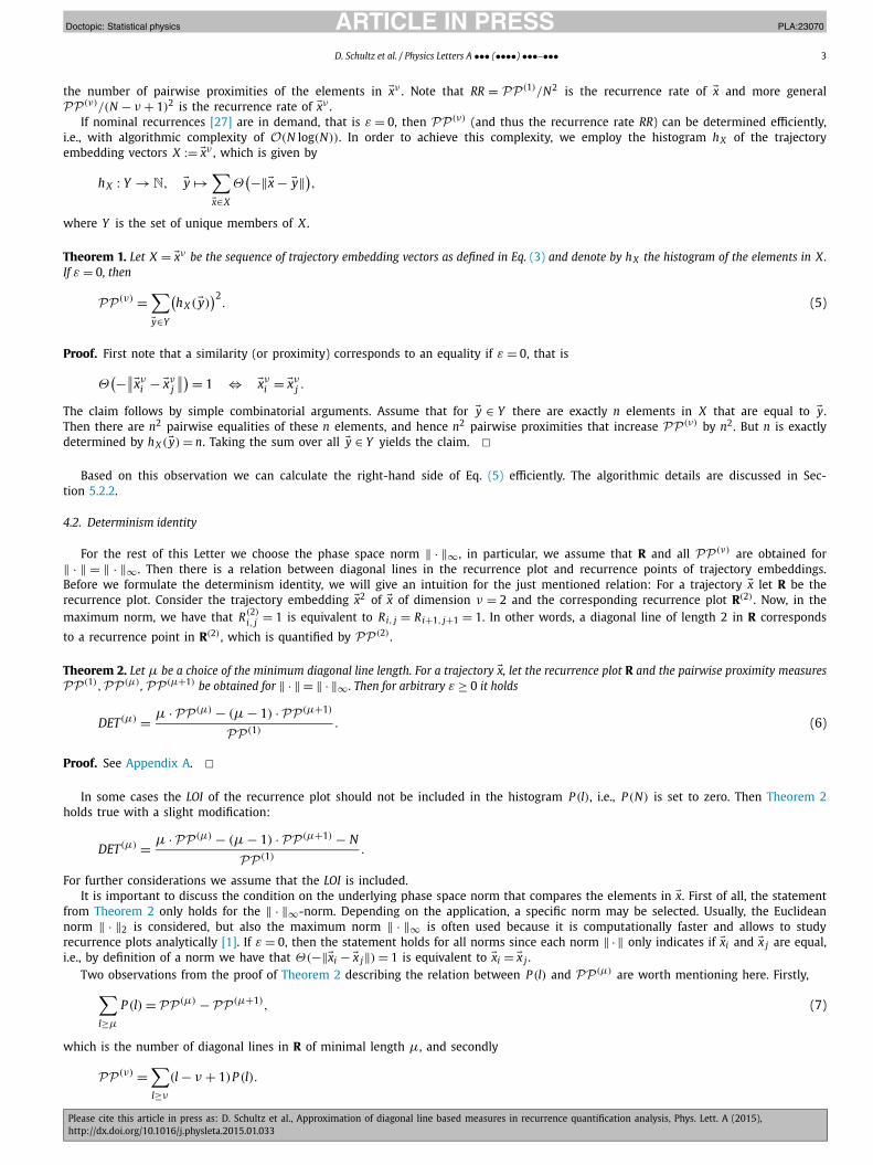
the number of pairwise proximities of the elements in �xν . Note that RR = PP(1)/N2 is the recurrence rate of �x and more general PP(ν)/(N − ν + 1)2 is the recurrence rate of �xν .

If nominal recurrences [27] are in demand, that is ε = 0, then PP(ν) (and thus the recurrence rate RR) can be determined efficiently, i.e., with algorithmic complexity of O(N log(N)). In order to achieve this complexity, we employ the histogram hX of the trajectory embedding vectors X := �xν , which is given by

hX : Y →N, �y →∑�x∈X

Θ(−‖�x − �y‖),

where Y is the set of unique members of X .

Theorem 1. Let X = �xν be the sequence of trajectory embedding vectors as defined in Eq. (3) and denote by hX the histogram of the elements in X. If ε = 0, then

PP(ν) =∑�y∈Y

(hX (�y)

)2. (5)

Proof. First note that a similarity (or proximity) corresponds to an equality if ε = 0, that is

Θ(−∥∥�xν

i − �xνj

∥∥) = 1 ⇔ �xνi = �xν

j .

The claim follows by simple combinatorial arguments. Assume that for �y ∈ Y there are exactly n elements in X that are equal to �y. Then there are n2 pairwise equalities of these n elements, and hence n2 pairwise proximities that increase PP(ν) by n2. But n is exactly determined by hX (�y) = n. Taking the sum over all �y ∈ Y yields the claim. �

Based on this observation we can calculate the right-hand side of Eq. (5) efficiently. The algorithmic details are discussed in Sec-tion 5.2.2.

4.2. Determinism identity

For the rest of this Letter we choose the phase space norm ‖ · ‖∞ , in particular, we assume that R and all PP (ν) are obtained for ‖ · ‖ = ‖ · ‖∞ . Then there is a relation between diagonal lines in the recurrence plot and recurrence points of trajectory embeddings. Before we formulate the determinism identity, we will give an intuition for the just mentioned relation: For a trajectory �x let R be the recurrence plot. Consider the trajectory embedding �x2 of �x of dimension ν = 2 and the corresponding recurrence plot R(2) . Now, in the maximum norm, we have that R(2)

i, j = 1 is equivalent to Ri, j = Ri+1, j+1 = 1. In other words, a diagonal line of length 2 in R corresponds to a recurrence point in R(2) , which is quantified by PP (2) .

Theorem 2. Let μ be a choice of the minimum diagonal line length. For a trajectory �x, let the recurrence plot R and the pairwise proximity measures PP(1), PP(μ) , PP(μ+1) be obtained for ‖ · ‖ = ‖ · ‖∞ . Then for arbitrary ε ≥ 0 it holds

DET(μ) = μ ·PP(μ) − (μ − 1) ·PP(μ+1)

PP(1). (6)

Proof. See Appendix A. �In some cases the LOI of the recurrence plot should not be included in the histogram P (l), i.e., P (N) is set to zero. Then Theorem 2

holds true with a slight modification:

DET(μ) = μ ·PP(μ) − (μ − 1) ·PP(μ+1) − N

PP(1).

For further considerations we assume that the LOI is included.It is important to discuss the condition on the underlying phase space norm that compares the elements in �x. First of all, the statement

from Theorem 2 only holds for the ‖ · ‖∞-norm. Depending on the application, a specific norm may be selected. Usually, the Euclidean norm ‖ · ‖2 is considered, but also the maximum norm ‖ · ‖∞ is often used because it is computationally faster and allows to study recurrence plots analytically [1]. If ε = 0, then the statement holds for all norms since each norm ‖ · ‖ only indicates if �xi and �x j are equal, i.e., by definition of a norm we have that Θ(−‖�xi − �x j‖) = 1 is equivalent to �xi = �x j .

Two observations from the proof of Theorem 2 describing the relation between P (l) and PP (μ) are worth mentioning here. Firstly,∑l≥μ

P (l) = PP(μ) −PP(μ+1), (7)

which is the number of diagonal lines in R of minimal length μ, and secondly

PP(ν) =∑

(l − ν + 1)P (l).

l≥ν

JID:PLA AID:23070 /SCO Doctopic: Statistical physics [m5G; v1.145; Prn:6/02/2015; 10:59] P.4 (1-15)

4 D. Schultz et al. / Physics Letters A ••• (••••) •••–•••

Fig. 1. The Lorenz attractor (left) from Eq. (12) and its discretization (right) for grid size parameter δ = 2.

By now, the identity in Theorem 2 does not provide a method to compute the determinism efficiently for general ε. However, if ε = 0, then PP (1), PP(μ) and PP (μ+1) can be calculated fast, as argued in Section 4.1, and then DET(μ) is a simple algebraic computation in terms of these quantities.

It is worth to mention that the relationship between the length of diagonal lines in the recurrence plot and the embedding dimension is of more fundamental nature. For example, the K2 entropy can be directly estimated from the recurrence plot using the diagonal line lengths [1] instead of the dimension of the embedding dimension [28].

5. Approximation of RQA

Approximations for RR and DET(μ) are presented that are computable in O(N log(N)). These approximative measures are obtained algorithmically, that means we do not calculate the recurrence plot. In Section 4, we have discussed the simplified case of ε = 0, where these measures are in the just mentioned complexity class. In this section we study the case of ε > 0, for which we propose a phase space discretization approach in order to approximate PP(ν) . The discretization will generate the situation of a zero threshold, which allows us to apply the results from Section 4.

5.1. Approximation method

We propose to discretize the phase space for a grid size parameter δ > 0 via

Φδ : Rn → Zn, �y → �y :=

⌊ �yδ

⌋, (8)

where n is an arbitrary natural number and �· is the component-wise round off operation. Applying Φδ to the trajectory �x leads to a partition of the phase space in hypercubes of size δ. Then we replace the similarity condition ‖�xν

i − �xνj ‖∞ ≤ ε by affiliation to the same

cube, i.e., by the condition �xνi = �xν

j . For convenience, we formulate this as a classification problem following the rules: �xνi and �xν

j are classified as

(1) Similar if Θ(−‖�xνi − �xν

j ‖∞) = 1.

(2) Dissimilar if Θ(−‖�xνi − �xν

j ‖∞) = 0.

This point of view leads to the idea of proposing an approximation of PP (ν) for ε > 0 by replacing Θ(ε − ‖�xνi − �xν

j ‖∞) by Θ(−‖�xνi −

�xνj ‖∞) in Eq. (4):

Definition 1. Let ε > 0. The approximations PP (ν)and DET

(μ)of PP(ν) and DET(μ) respectively are defined as

PP(ν) :=N−ν+1∑

i, j=1

Θ(−∥∥�xν

i − �xνj

∥∥∞),

DET(μ) := μ · PP(μ) − (μ − 1) · PP(μ+1)

PP(1).

The crucial difference between PP (ν) and PP (ν)is that for the latter the similarity threshold is zero. In this case PP (ν)

can be calculated algorithmically by applying Theorem 1 for X = �xν (rather than X = �xν ). Then DET

(μ)simply utilizes PP (ν)

for ν = 1, μ, μ + 1in Theorem 2.

At this point we emphasize that the approximation method and resulting approximation errors are based on the discretization only. Once we have discretized the data and use a threshold that is zero, the results from Section 4 are applied in order to calculate the RQA measures efficiently. Quantifying the discretized data with the use of a recurrence plot will lead to the exact same result. An example of a discretization is illustrated in Fig. 1. The reader is invited to follow the example in Appendix B parallel to further investigations.

JID:PLA AID:23070 /SCO Doctopic: Statistical physics [m5G; v1.145; Prn:6/02/2015; 10:59] P.5 (1-15)

D. Schultz et al. / Physics Letters A ••• (••••) •••–••• 5

Fig. 2. Classification situations for x ∈ [1.5δ, 2δ) and δ = 2ε. In this one-dimensional case, the hypercubes are simply intervals in R. Here, x = 1 and thus x belongs to the cube no. 1. For y ∈R, in fact x and y are similar if y ∈ [x − ε, x + ε], hence x and y are not classified correctly if y ∈ [δ, x − ε) or y ∈ [2δ, x + ε].

5.2. Investigation of the approximation method

We explore the phase space discretization from Section 5.1 and its impact on the approximation of PP (ν) . Recall that we formulated the approximation procedure as a classification problem.

Denote by (x, y) ∼ C(S, T ) the situation that x and y are classified as belonging to class S where they are in fact in class T . Then, if Smeans ‘similar’, there are four classification situations (compare with Fig. 2), namely

(x, y) ∼ C(S, S) ⇔ x = y and ‖x − y‖∞ ≤ ε.

(x, y) ∼ C(¬S,¬S) ⇔ x �= y and ‖x − y‖∞ > ε.

(x, y) ∼ C(S,¬S) ⇔ x = y and ‖x − y‖∞ > ε.

(x, y) ∼ C(¬S, S) ⇔ x �= y and ‖x − y‖∞ ≤ ε.

For �xν we conclude the following observations.

1. If for each pair (�xνi , �xν

j ) ∼ C(S, S) or (�xνi , �xν

j ) ∼ C(¬S, ¬S), then clearly PP(ν) =PP(ν) . However,

2. if (�xνi , �xν

j ) ∼ C(¬S, S), the similarity of (�xνi , �xν

j ) increases PP (ν) , but not PP (ν); and

3. if (�xνi , �xν

j ) ∼ C(S, ¬S), the dissimilarity of (�xνi , �xν

j ) increases PP (ν), but not PP (ν) .

Therefore these two types of errors satisfy a mutual canceling property, and if the number of C(¬S, S)-errors equals the number of C(S, ¬S)-errors, then even PP(ν) =PP (ν) follows.

From these considerations we establish the choice of δ = 2ε.

5.2.1. The discretization parameter δThe grid size δ of the discretization determines which elements are classified as similar and thus has to be chosen carefully. If we

make no further assumptions to the data, by intuition δ = 2ε is a reasonable choice since the similarity diameter in phase space is 2ε, and moreover the different error zones have exactly the same measure (see Fig. 2). This also means that δ = 2ε is optimal and leads to nearly zero approximation error if the values of the time series x are independent uniformly distributed (on an appropriate interval). Note that ε > 0 was supposed implicitly since δ > 0 is required in Eq. (8). If ε = 0, then no discretization is applied, and in fact not necessary since from Theorem 1 follows that the exact quantity PP (ν) can be calculated efficiently. Let us now discuss the algorithmic details.

5.2.2. AlgorithmsThe previous findings are used to provide algorithms for the calculation of the approximations from Definition 1; and in case of ε = 0

for fast calculation of the exact measures PP (ν) and DET(μ) . Since the methods for fast processing of the approximations and the exact terms are identical, for ε = 0 we now denote �xν := �xν and state algorithms for PP (ν)

and DET(μ)

, given an arbitrary ε ≥ 0.As already observed in Section 4.1 it is enough to find the histogram hX of the (discretized) sequence of trajectory embedding vectors

X := �xν , since then PP (ν)is given by

PP(ν) =∑�y∈Y

(hX (�y)

)2, (9)

where Y is again the set of unique members of X . Technically, this may be achieved by assigning unique identifiers to the elements in X , i.e., we are interested in integers J1, . . . , J N−ν+1, such that

�xνi = �xν

j ⇔ J i = J j for all i, j,

and charge the histogram of these identifiers (compare with Algorithm 1). The calculation of DET(μ)

is presented in Algorithm 2. Finally, the efficiency of these procedures is argued in Section 5.2.3.

Recall the designations. For more clarity, we eliminate the vector arrows in the algorithms, i.e., x := �x is the trajectory of length N , ε ≥ 0 is the similarity threshold, μ the minimum diagonal line length, ν is the trajectory embedding dimension and xν := �xν is the matrix that consists of the rows xν

j := �xνj , j = 1, . . . , N −ν +1. We emphasize that the algorithm is not restricted to one-dimensional trajectories x,

provided appropriate implementation. In Section 6 we provide MATLAB® code that handles multi-dimensional data.

JID:PLA AID:23070 /SCO Doctopic: Statistical physics [m5G; v1.145; Prn:6/02/2015; 10:59] P.6 (1-15)

6 D. Schultz et al. / Physics Letters A ••• (••••) •••–•••

Algorithm 1 Fast calculation of PP (ν)(or PP(ν) if ε = 0).

1: procedure PPapprox(x, ε, ν)2: if ε = 0 then � No discretization, method is exact.3: x ← x4: else � Discretization of phase space, Eq. (8).5: δ ← 2ε6: x ← Φδ(x)7: end if8: xν ← apply_trajectory_embedding(x, ν)

9: J = ( J1, . . . , J N−ν+1) ← find_unique_row_ IDs(xν )

10: h ← histogram( J )

11: PP (ν) ← ∑i h2

i12: end procedure

Algorithm 2 Fast calc. of DET(μ)

(or DET(μ) if ε = 0).1: procedure DETapprox(x, ε, μ)2: PP (1) ← PPapprox(x, ε, 1)

3: PP (μ) ← PPapprox(x, ε, μ)

4: PP (μ+1) ← PPapprox(x, ε, μ + 1)

5: DET(μ) ← (μ ·PP (μ) + (μ − 1) ·PP (μ+1))/PP (1)

6: end procedure

5.2.3. Complexity analysisWe specify the computational complexity by means of the number of vector-level comparisons. This conforms with the specification

of the complexity of a recurrence plot computation. Here O(N2) indicates the number of distance calculations between pairs of vectors, regardless of their dimension. Denote by Oc and Os the computational and space complexity respectively.

Theorem 3. Let ν and μ ∈N be fixed choices of the trajectory embedding dimension and the minimum diagonal line length, respectively.

(i) The complexity classes of the approximations PP(ν)and DET

(μ)are Oc(N log(N)) and Os(N).

(ii) If ε = 0, then the exact terms PP(ν) and thus the exact RQA-measures RR and DET(μ) are in the complexity classes Oc(N log(N)) and Os(N), given an arbitrary phase space norm || · ||.

Proof. We investigate the complexity of Algorithm 1. The complexity class of Algorithm 2 is clearly identical.(i) It is easy to verify that the operations in lines 2–8 are in Oc(N) and Os(N). The main cost is taken by line 9. One way to find

unique identifiers for the rows of �xν is based on sorting the rows lexicographically. Recall that the rows are trajectory embedding vectors of dimension d ·ν . Provided a fast comparison-based sorting algorithm, e.g., Quicksort, we need Oc(N log(N)) vector-level comparisons of the trajectory embedding vectors in order to sort them. For completeness, each comparison of a pair of vectors needs at most d · ν scalar-level comparisons in order to determine which vector is smaller with respect to the lexicographic order. However, as mentioned above, we specify the complexity at vector-level. Also note that there are sorting algorithms at scalar-level that are faster than Oc(dνN log(N)) [29]. Once the rows are sorted, it is enough to incrementally iterate the rows in order to assign an ID J i to each row �xν

i , leading to a complexity of Oc(N) for the assignment step. Summarizing, the overall complexity in line 9 is Oc(N log(N)). In line 10 it is enough to incrementally count equal entries in J , giving Oc(N). Finally the complexity in line 11 is Oc(N) since n ≤ N , where n is the length of the vector h. Altogether the dominating complexity classes are Oc(N log(N)) and Os(N).

(ii) Let ε = 0. Determine PP (1) using Algorithm 1 and set RR = PP(1)/N2. Compute DET(μ) using Algorithm 2. By Theorems 1 and 2 these expressions coincide with the exact RQA-measures. As already mentioned in Section 4.2, if ε = 0, then the identities hold for an arbitrary phase space norm since each norm only indicates whether two elements in phase space are equal. The claim on the complexity classes is proven in the first part. �

We remark that sorting the rows lexicographically is not the only possibility. One could, for instance, use a hash function that maps the embedding vectors to R in order to get the identifiers for the embedding vectors and then apply a simple one-dimensional sorting algorithm to find the histogram incrementally. However, such hash functions do not guarantee unique identifiers since they are not injective in general.

5.2.4. Worst case errorAs shown in Theorem 3, if ε = 0, then PP (ν) can be calculated exactly and efficiently. If ε > 0, the approximation PP(ν)

of PP(ν)

satisfies the following estimates.

Theorem 4. Let ε > 0 and δ = 2ε. In d-dimensional phase space it holds

1

2dνPP(ν) ≤ PP(ν) ≤ 2dνPP(ν).

Proof. Denote m = dν . The lower bound is reached if the number of C(¬S, S)-errors is maximal. Let �y be a vertex of the discretization lattice. In m-dimensional space there are 2m adjoint hypercubes surrounding �y. Hence it is possible to place 2m points �xi , each in another cube, such that ‖�y − �xi‖∞ ≤ ε/2 for all i. It follows that ‖�xi − �x j‖∞ ≤ ε for all i, j. Hence each pair (�xi, �x j) is similar, but by construction

JID:PLA AID:23070 /SCO Doctopic: Statistical physics [m5G; v1.145; Prn:6/02/2015; 10:59] P.7 (1-15)

D. Schultz et al. / Physics Letters A ••• (••••) •••–••• 7

classified as dissimilar if i �= j. In this case we have PP (ν) = (2m)2 and PP (ν) = 2m . The argument is finished since placing additional points only leads to a reduction of the number of C(¬S, S)-errors.

The upper bound follows in a similar manner by producing errors of type C(S, ¬S). �By now the bounds are shown to be existent (hence the theorem is true) but not that they are sharp. One would have to show

that there is a trajectory whose embedding vectors are constructed as above. For ν = 2 and d = 1 an appropriate trajectory is given by �x = (η, η, −η, −η, η), where η < ε/2. The four resulting trajectory embedding vectors of �x satisfy the above construction. For general ν and d this becomes more technical, but we think that this investigation is unnecessary at this point. It is more interesting how the approximation error behaves empirically.

5.2.5. Empirical approximation error

As seen in Section 5.2.4 the bounds of the approximation error of PP(ν)are rather large and monotonic in ν . However, the construc-

tions given in the proof of Theorem 4 to reach these bounds are very specific.

In this section we study the approximation errors of PP (ν)and DET

(μ)empirically. For this sake the relative mean errors of 100

realizations, designed as follows, are determined. For each experiment the autoregressive process �x = (x1, . . . , xN ), with

xi = axi−1 + bηi, i = 2, . . . , N, (10)

is generated for N = 1000 time steps, where x1 = 0, a, b are fixed values that are chosen randomly independent uniformly distributed on [0, 1] and η is a vector of Gaussian white noise. Then the approximations are determined by the algorithms from Section 5.2.2 and the exact quantities PP (ν) and DET(μ) are calculated by the classical method in order to specify the accuracy of the approximations. The results are illustrated in Fig. 3 for several combinations of ν (resp. μ) and ε, where the height of the bars corresponds to the mean error and the color of the bars corresponds to the value PP (ν) and DET(μ) , respectively. It is customary to select ε as a few percent of the phase space diameter [1,30], which in this case is given by range(�x) = max(�x) − min(�x).

We observe that the approximation errors are basically increasing in ν (resp. μ) and ε. However, most of the combinations of ν (resp. μ) and ε have little relevance. First, if ε is small and ν (resp. μ) is large, the probability to find recurrences is low. Consequently the bars in Fig. 3(a) are of deep blue color. Therefore the low error in this area is an artefact. Conversely, if ν (resp. μ) is small and ε is large, too many recurrences are found, resulting in red colors. Reasonable choices of ν (resp. μ) and ε are indicated by colors in the range from blue-green to orange-red in Fig. 3(a).

As an example, assume that we want to determine the recurrence rate and the determinism of the trajectory �x. For the calculation of the determinism, a minimal line length of μ = 2 is sufficient, because for the autoregressive process we do not expect much effect of tangential motion or sampling [1]. Then for all sensible values of ε, i.e., from 0 to 8 percent of the range, we obtain mean approximation errors below 1.4% for the recurrence rate and below 2.7% for the determinism.

It should be noticed that we have investigated one-dimensional trajectories �x that are not reconstructed by time series embedding. However, the trajectory embedding of dimension ν can also be imagined as time series embedding if we postulate that �x is the time series and �xν is the trajectory, which is obtained from �x by time series embedding with time delay 1 and embedding dimension ν . Then Fig. 3(a) reflects the approximation errors of the recurrence rate of �xν , which is given by PP(ν)/(N −ν + 1)2. The essence of this technical point of view is that the approximation errors increase if the dimension of the trajectory increases. We also observe this in the experiment from Section 6 for the 3-dimensional Lorenz attractor, see Table 2.

6. Execution time of Algorithm 1

We compare the execution times of PP and its approximation PP on a consumer computer (2.3 GHz Intel Core i7 quad core processor, 16 GB 1600 MHz DDR3 RAM). Since execution times do not only depend on the algorithm, but also on the implementation, we provide MATLAB® code. Note that, however, this code uses standard MATLAB® routines and may be strongly optimized by the MATLAB® compiler.

We evaluate two systems, the autoregressive process

x1 = 0, xi = 0.57xi−1 + 0.24ηi, i = 2, . . . ,100,000,000 (11)

and the well-known 3-dimensional Lorenz system (see Fig. 1)

x = a(y − x), y = x(b − z) − y, z = xy − cz (12)

for the parameters a = 10, b = 28, c = 8/3. Then these systems are truncated according to the values of N as listed in the tables of results, Tables 1 and 2, and Fig. 4, and processed by the routines. The threshold ε was chosen for each N separately as 7% of the phase space diameter and no embedding is applied, i.e. m = 1 in the following MATLAB® function.

MATLAB® code for PP

function pp = PPapprox( x, eps, m)[N,d] = size(x);if eps > 0 % discretize if eps > 0

x = floor(x/(2*eps));endX = zeros(N-m+1,d*m); % apply trajectory embeddingfor i = 1:m

X(:,d*(i-1)+1:d*i) = x(i:N-(m-i),:);

JID:PLA AID:23070 /SCO Doctopic: Statistical physics [m5G; v1.145; Prn:6/02/2015; 10:59] P.8 (1-15)

8 D. Schultz et al. / Physics Letters A ••• (••••) •••–•••

Fig. 3. Relative mean errors obtained from 100 autoregressive process realizations. The bar color in (a) indicates the value of the exact recurrence rate RR(ν) = PP (ν)/(N −ν +1)2 of the embedded trajectory �xν . The bar color in (b) reflects the exact determinism DET(μ) of the trajectory �x, given a minimum diagonal line length μ. (For interpretation of the references to color in this figure, the reader is referred to the web version of this article.)

end[u,~,iu] = unique(X,’rows’); % find row ID’s iuh = hist(iu,size(u,1)); % find histogram of row ID’spp = sum(h.^2);end

MATLAB® code for PP

function pp = PP( x, eps)R = pdist2(x,x,’chebychev’) <= eps; % calculate recurrence plotpp = nnz(R); % count nonzerosend

Since the available memory on the computer was 12 GB, we limited the data size for the exact measure PP . Indeed a single recurrence plot for N = 40,000 consumes about 12 GB of RAM, provided double precision and no storage optimization. For N = 100,000 even about 75 GB of memory would be required. The results give numerical evidence for the complexity we have proved in Theorem 3 and reflect

JID:PLA AID:23070 /SCO Doctopic: Statistical physics [m5G; v1.145; Prn:6/02/2015; 10:59] P.9 (1-15)

D. Schultz et al. / Physics Letters A ••• (••••) •••–••• 9

Table 1Mean execution times obtained from 10 realizations of the autoregressive process (11) for different time series length N . The approximation error is again the mean over the relative errors |PP − PP|/PP .

N Execution time PP (s) Execution time PP (s) Approximation error

100 0.0552 0.0005 0.02751000 0.0078 0.0005 0.0104

10,000 0.9058 0.0018 0.009820,000 3.7314 0.0158 0.009830,000 8.3865 0.0233 0.009635,000 13.7078 0.0131 0.0092

100,000 – 0.0169 –1,000,000 – 0.1912 –

10,000,000 – 2.2587 –100,000,000 – 28.5899 –

Table 2Mean execution times obtained from 10 realizations of the Lorenz system (12) for different time series length N . The approximation error is again the mean over the relative errors |PP − PP|/PP .

N Execution time PP (s) Execution time PP (s) Approximation error

100 0.0513 0.0009 0.04711000 0.0077 0.0006 0.3655

10,000 0.9071 0.0052 0.288520,000 3.7200 0.0074 0.264630,000 8.2962 0.0117 0.2746

100,000 – 0.0396 –1,000,000 – 0.3645 –

Fig. 4. Visual representation of the execution times from Tables 1 and 2 in log scale.

the large difference between O(N2) and O(N log(N)) for increasing N . For example the ratio of execution times for the autoregressive process with N = 35,000 is about 1.046. Moreover, the algorithm is very fast for extreme large data and the approximation error decreases slightly with growing N . In Table 2 the small approximation error for N = 100 is due to the short and hence almost linear attractor. As expected, the other errors of the Lorenz experiment are higher since the attractor is 3-dimensional.

7. Application to transition detection

7.1. Introduction to the problem

Assume that we are given a time series or a stream x = (x1, x2, x3, . . .) which changes its dynamics at unknown time segments. It has been shown that the determinism DET(μ) is able to find these periods [5,6,31]. For this, the time series is analyzed window-wise for a window size w and step size s, leading to a sequence D of determinism-values. More precisely, D( j) contains the determinism of the sub-sequence (xs· j, . . . , xs· j+w−1), j = 1, 2, 3, . . . . A transition in the dynamics is indicated when the system leaves its typical dynamical behavior, in this case its typical range of the window-wise determinism values [6]. The bounds of this range are referred to as confidence levels. An example of a graph of D is illustrated as red line in Fig. 5. In the gray marked area the system from the upper plot changes its dynamics (details in Section 7.2) and consequently D exceeds its upper confidence bound, which is represented by the dashed red line.

In this section we compare our proposed approximation DET(μ)

to the exact measure DET(μ) for the problem of identifying transition times. Again, we consider a minimal line length of μ = 2. It remains to select ε. For each window ε is determined separately such that the recurrence rate is a small fraction, e.g., 0.1 [6]. This leads to a constant (in time index i) denominator in Eq. (2) accentuating the behavior of the changes in P (l).

JID:PLA AID:23070 /SCO Doctopic: Statistical physics [m5G; v1.145; Prn:6/02/2015; 10:59] P.10 (1-15)

10 D. Schultz et al. / Physics Letters A ••• (••••) •••–•••

Fig. 5. Example from the transition experiment. The system of the upper plot is generated as described in Section 7.2. The lower graphic shows the window-wise determinism sequence D and its approximation D. The dashed lines are the confidence levels.

Table 3Mean transition errors obtained from 100 realizations as described in Section 7.2. The left/right transition error is defined as the absolute deviation from time index 1300/1800.

Measure Left transition error Right transition error

DET(2) 61.25 64.75

DET(2)

85.00 45.50

7.2. Autoregressive process with changing parameters

The experiment is inspired by [6]. We evaluate 100 realizations employing autoregressive processes of order 2,

xi = axi−1 − bxi−2 + cηi .

The test time series is initially generated for x1 = x2 = 0 and a = 1.8, b = 0.972, c = 0.64 for 1300 time steps. Then the parameters change for a period of 500 time steps to a = 1.85, b = 0.917, c = 0.76. Finally the system returns to the initial parameters and stops at time step 3500. The resulting time series x is then analyzed for a window size w = 400 and step size s = 25.

In the exact case D contains the values of DET(2) , where ε is chosen such that the recurrence rate PP(1)/w2 is 0.1. In the approxima-

tive case D contains the values of DET(2)

, where ε is chosen such that the approximate recurrence rate PP (1)/w2 is 0.1.

In order to find the upper confidence level, we assume that the system with initial parameters is observed for N = 100,000 time steps and the distribution of the (approximate) determinism values for the windows is charged. We choose as transition level the 99.95%-quantile of those distributions, leading to a confidence level of 0.4425 for DET(2) and 0.4523 for DET

(2). For the evaluation the

time points of exceeding and falling below these levels are compared to the actual transition time at 1300 and 1800. The results reveal that our fast approximation performs as well as the slow exact method (Table 3).

7.3. Transitions in the logistic map

We briefly illustrate that the approximate determinism DET is also able to find transitions in the logistic map [20,31]

xi+1 = axi(1 − xi), (13)

with control parameter a in the range [3.6, 3.8] and x1 = 0.7. In the simulations we observed that the quality of the approximation is sensitive to ε. We found that a rather small threshold is beneficial. More precisely, we selected ε for each a separately such that the recurrence rate resp. the approximate recurrence rate is 0.01. Fig. 6 confirms that DET has the capability to find dynamical transitions. For N = 10,000 and 400 iterative values of a we observed that the approximation was about 124 times as fast as the exact computation, including all iterations and determinations of ε (24.5 s for approximation, 3041.7 s for exact determinism).

8. Other RQA measures

Using PP (ν) it is possible to specify identities for other diagonal line based RQA-measures. Detailed analysis of those is out of the scope of this work, but we briefly state the formulas in this section. In the following equations the left-hand side is the classical definition and the right-hand side is the identity in terms of PP (ν) . As before, μ denotes the minimum diagonal line length, the phase space norm is ‖ · ‖∞ and the LOI is included unless otherwise stated.

For the ratio RATIO(μ) between DET(μ) and RR, we get

N2

∑l≥μ lP (l)

(∑

l≥1 lP (l))2= N2 μPP(μ) − (μ − 1)PP(μ+1)

(PP(1))2.

Due to Eq. (7), the averaged diagonal line length L(μ) is given by

JID:PLA AID:23070 /SCO Doctopic: Statistical physics [m5G; v1.145; Prn:6/02/2015; 10:59] P.11 (1-15)

D. Schultz et al. / Physics Letters A ••• (••••) •••–••• 11

Fig. 6. Bifurcation diagram of the logistic map (13) and its dynamics. We observe multiple chaos-period transitions that are found by both measures, DET and its approxima-tion DET . For clarity, the peaks of DET are increased from 1 to 1.05.∑

l≥μ lP (l)∑l≥μ P (l)

= μPP(μ) − (μ − 1)PP(μ+1)

PP(μ) −PP(μ+1),

and the length of the longest diagonal line Lmax (excluding the LOI, i.e., P (N) := 0), determined by

max{l∣∣ P (l) �= 0

} = min{ν

∣∣ PP(ν) = N − ν + 1} − 1,

can be found by binary search in O(log(N)) iterations since ν →PP (ν) is monotonically decreasing.Finally we should remember that these expressions can be calculated exactly and efficiently if ε = 0; and in case of ε > 0 the measures

can be approximated by replacing PP by PP . In both cases Algorithm 1 determines the pairwise proximity measures efficiently. For Lmaxthe resulting computational complexity is O(N log2(N)). All other approximative measures are in O(N log(N)), whereas the complexity of the classical measures is O(N2) [11].

9. Conclusions

We have shown that the recurrence rate and many diagonal line based RQA-measures can be calculated efficiently, i.e., in O(N log(N)) if the similarity threshold ε is zero. For the case ε > 0 we have introduced approximations of these measures that are based on phase space discretization and a relation between the histogram of the diagonal line lengths P (l) and the introduced pairwise proximity measures of trajectory embeddings. For small embedding dimension ν or minimum diagonal line length μ the proposed approximations are very close to the exact quantities in our experiments with one-dimensional data, while execution times and memory consumption are significantly lower. However, we suggest to compare the approximations with the exact measures since the accuracy strongly depends on the data under study. In particular, if the trajectory is multi-dimensional the approximation error may increase. We also recommend to keep ε as small as possible since it determines the grid size of the discretization. In general, a small grid size leads to gentle discretization and, consequently, causes low approximation errors.

The proposed approximation of diagonal line based RQA-measures, with its substantially improved time and space complexity, makes it possible to efficiently analyze the nonlinear behavior of fast data streams and long data sequences, even if the computations are performed on an embedded system with limited processing power and memory. The online analysis of data streams is critical for medical applications that monitor vital functions, such as brain and heart activity. The offline processing of long data sequences is important for analyzing historical measurements, e.g., hourly weather variability, which usually cause expensive or even intractable computations if traditional RQA-measures without approximation techniques are employed.

In future work we aim at investigating data-adopted discretization lattices and their ability to improve the approximation accuracy. Furthermore, we plan to study under which conditions the ratio DET(�x)/DET(�x) stays stable (i.e. nearly constant) for changing �x. Clearly, if the approximation error is small, this stability is present. But if the error is large, this stability would still allow us to compare dynamics rather than determine dynamics, which is sufficient for many applications, e.g., transition detection.

Appendix A. Proof of the determinism identity

Proof of Theorem 2. Let �x = (�x1, . . . , �xN ) be a d-dimensional phase space trajectory (d ∈ N) of length N and the similarity threshold ε ≥ 0as well as the minimum diagonal line length μ ∈ N be given. Assume that ‖ · ‖∞ is the underlying phase space norm, i.e., the recurrence plot of �x is given by

Ri, j = Θ(ε − ‖�xi − �x j‖∞

), i, j = 1, . . . , N,

and for all ν ∈ N the pairwise proximity measures PP(ν) are defined as

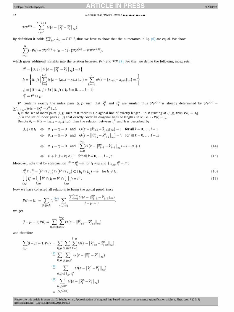
JID:PLA AID:23070 /SCO Doctopic: Statistical physics [m5G; v1.145; Prn:6/02/2015; 10:59] P.12 (1-15)

12 D. Schultz et al. / Physics Letters A ••• (••••) •••–•••

PP(ν) =N−ν+1∑

i, j=1

Θ(ε − ∥∥�xν

i − �xνj

∥∥∞).

By definition it holds ∑N

i, j=1 Ri, j =PP (1) , thus we have to show that the numerators in Eq. (6) are equal. We show

N∑l=μ

l · P (l) = PP(μ) + (μ − 1) · (PP(μ) −PP(μ+1)),

which gives additional insights into the relation between P (l) and PP (7). For this, we define the following index sets.

Iμ = {(i, j)

∣∣ Θ(ε − ∥∥�xμ

i − �xμj

∥∥∞) = 1

}Il =

{(i, j)

∣∣∣ l−1∑k=0

Θ(ε − ‖xi+k − x j+k‖∞

) =l∑

k=−1

Θ(ε − ‖xi+k − x j+k‖∞

) = l

}Jl = {

(i + k, j + k)∣∣ (i, j) ∈ Il,k = 0, . . . , l − 1

}Iμl = Iμ ∩ Jl

Iμ contains exactly the index pairs (i, j) such that �xμi and �xμ

j are similar, thus PP (μ) is already determined by PP(μ) =∑(i, j)∈Iμ Θ(ε − ‖�xμ

i − �xμj ‖∞).

Il is the set of index pairs (i, j) such that there is a diagonal line of exactly length l in R starting at (i, j), thus P (l) = |Il|.J l is the set of index pairs (i, j) that exactly cover all diagonal lines of length l in R, i.e., l · P (l) = | J l|.

Denote θk = Θ(ε − ‖xi+k − x j+k‖∞), then the relation between Iμl and Il is described by

(i, j) ∈ Il ⇔ θ−1 = θl = 0 and Θ(ε − ‖�xi+k − �x j+k‖∞

) = 1 for all k = 0, . . . , l − 1

⇔ θ−1 = θl = 0 and Θ(ε − ∥∥�xμ

i+k − �xμj+k

∥∥∞) = 1 for all k = 0, . . . , l − μ

⇔ θ−1 = θl = 0 andl−μ∑k=0

Θ(ε − ∥∥�xμ

i+k − �xμj+k

∥∥∞) = l − μ + 1 (14)

⇔ (i + k, j + k) ∈ Iμl for all k = 0, . . . , l − μ. (15)

Moreover, note that by construction Iμl1 ∩ Iμl2 = ∅ for l1 �= l2 and⋃

l≥μ Iμl = Iμ:

Iμl1 ∩ Iμl2 = (Iμ ∩ Jl1

) ∩ (Iμ ∩ Jl2

) ⊂ ( Jl1 ∩ Jl2) = ∅ for l1 �= l2, (16)⋃l≥μ

Iμl =⋃l≥μ

Iμ ∩ Jl = Iμ ∩⋃l≥μ

Jl = Iμ. (17)

Now we have collected all relations to begin the actual proof. Since

P (l) = |Il| =∑

(i, j)∈Il

1(14)=

∑(i, j)∈Il

∑l−μk=0 Θ(ε − ‖�xμ

i+k − �xμj+k‖∞)

l − μ + 1,

we get

(l − μ + 1)P (l) =∑

(i, j)∈Il

l−μ∑k=0

Θ(ε − ∥∥�xμ

i+k − �xμj+k

∥∥∞)

and therefore

∑l≥μ

(l − μ + 1)P (l) =∑l≥μ

∑(i, j)∈Il

l−μ∑k=0

Θ(ε − ∥∥�xμ

i+k − �xμj+k

∥∥∞)

(15)=∑l≥μ

∑(i, j)∈Iμl

Θ(ε − ∥∥�xμ

i − �xμj

∥∥∞)

(16)=∑

(i, j)∈⋃l≥μ Iμl

Θ(ε − ∥∥�xμ

i − �xμj

∥∥∞)

(17)=∑

(i, j)∈Iμ

Θ(ε − ∥∥�xμ

i − �xμj

∥∥∞)

= PP(μ).

JID:PLA AID:23070 /SCO Doctopic: Statistical physics [m5G; v1.145; Prn:6/02/2015; 10:59] P.13 (1-15)

D. Schultz et al. / Physics Letters A ••• (••••) •••–••• 13

Fig. 7. Recurrence plots (RPs) of the recurrence matrices from Eq. (19) for ν = 1, 2, 3, illustrated in black, blue, orange, respectively. (For interpretation of the references to color in this figure, the reader is referred to the web version of this article.)

Rearranging this equation leads to∑l≥μ

lP (l) = PP(μ) + (μ − 1)∑l≥μ

P (l), (18)

and it remains to show that

PP(μ) −PP(μ+1) =∑l≥μ

P (l).

But this already follows by applying (18) for μ and μ + 1:

PP(μ) −PP(μ+1) =∑l≥μ

lP (l) − (μ − 1)∑l≥μ

P (l) −( ∑

l≥μ+1

lP (l) − μ∑

l≥μ+1

P (l)

)

=∑l≥μ

lP (l) − (μ − 1)∑l≥μ

P (l) −(∑

l≥μ

lP (l) − μP (μ) − μ∑l≥μ

P (l) + μP (μ)

)=

∑l≥μ

P (l). �

Appendix B. Example

Assume that we want to compute the determinism of the sample trajectory �x = (0.5, 0.8, 0.4, 0.6, 0.8, 0.4, 0.9), given a similarity threshold ε = 0.1. First we consider the recurrence plots

R(ν)i, j := Θ

(ε − ∥∥�xν

i − �xνj

∥∥∞), R(ν)

i, j := Θ(−∥∥�xν

i − �xνj

∥∥∞)

(19)

of the embedded (3) trajectory �xν and its discretization �xν = Φδ(�xν), where δ = 0.2 (see (8) and Section 5.2.1). The embedded trajectories and the corresponding recurrence plots are illustrated in Fig. 7 for several embedding dimensions ν = 1, 2, 3 in black, blue, and orange color, respectively. For example the recurrence plots for ν = 2 comprise the recurrences marked by blue color, the black only highlighted entries are no recurrences for ν = 2.

For ν = 1 (write R = R(1)) we observe that R1,4 = 1, but R1,4 = 0. That means the pair (0.5, 0.6) is similar, i.e.,

|0.5 − 0.6| = 0.1 ≤ ε,

but classified as dissimilar:

Φδ(0.5) =⌊

0.5

0.2

⌋= 2 �= 3 =

⌊0.6

0.2

⌋= Φδ(0.6).

Due to symmetry the pairs (0.5, 0.6) and (0.6, 0.5) lead to C(S, ¬S)-errors (see Section 5.2). For all other pairs the classified and actual similarity statements coincide.

Recall that the determinism is the ratio between the number of points on diagonal lines and all points in the recurrence plot. For the trajectories �x = �x1 and �x = �x1 we obtain by counting the black structures in the recurrence plots:

DET(2) = 17 ≈ 0.81, DET(2) = 15 ≈ 0.79. (20)

21 19

JID:PLA AID:23070 /SCO Doctopic: Statistical physics [m5G; v1.145; Prn:6/02/2015; 10:59] P.14 (1-15)

14 D. Schultz et al. / Physics Letters A ••• (••••) •••–•••

Fig. 8. Trajectory embedding vectors with assigned IDs (left) and corresponding histograms (right).

Of course we have calculated the approximation inefficiently by employing the recurrence plot R. Using Theorem 2 and Algorithm 1

we may compute DET(2)

algorithmically.Following Algorithm 1 we assign unique identifiers to the rows of �xν . Note that in Fig. 8 the �xν are transposed, hence in this case we

are interested in unique columns. The histograms of the identifiers (col_ID) are charged and due to Theorem 1 we calculate (compare with Fig. 8)

• PP(1) = 32 + 32 + 12 = 19• PP(2) = 22 + 22 + 12 + 12 = 10• PP(3) = 12 + 12 + 12 + 12 + 12 = 5

Finally, using Definition 1 (which is based on Theorem 2) we get the same result as before in Eq. (20):

DET(2) = 2 · PP(2) − (2 − 1) · PP(3)

PP(1)= 15

19≈ 0.79.

References

[1] N. Marwan, M.C. Romano, M. Thiel, J. Kurths, Recurrence plots for the analysis of complex systems, Phys. Rep. 438 (5–6) (2007) 237–329, http://dx.doi.org/10.1016/j.physrep.2006.11.001.

[2] C.L. Webber Jr., N. Marwan, Recurrence Quantification Analysis – Theory and Best Practices, Springer, Heidelberg, 2015.[3] C.L. Webber Jr., N. Marwan, A. Facchini, A. Giuliani, Simpler methods do it better: success of recurrence quantification analysis as a general purpose data analysis tool,

Phys. Lett. A 373 (2009) 3753–3756, http://dx.doi.org/10.1016/j.physleta.2009.08.052.[4] N. Marwan, J. Kurths, Comment on “Stochastic analysis of recurrence plots with applications to the detection of deterministic signals” by Rohde et al. [Physica D 237

(2008) 619–629], Physica D 238 (16) (2009) 1711–1715, http://dx.doi.org/10.1016/j.physd.2009.04.018.[5] A. Facchini, C. Mocenni, N. Marwan, A. Vicino, E.B.P. Tiezzi, Nonlinear time series analysis of dissolved oxygen in the Orbetello Lagoon (Italy), Ecol. Model. 203 (3–4)

(2007) 339–348, http://dx.doi.org/10.1016/j.ecolmodel.2006.12.001.[6] N. Marwan, S. Schinkel, J. Kurths, Recurrence plots 25 years later – gaining confidence in dynamical transitions, Europhys. Lett. 101 (2013) 20007, http://dx.doi.org/

10.1209/0295-5075/101/20007.[7] S. Spiegel, J.-B. Jain, S. Albayrak, A Recurrence Plot-Based Distance Measure, Springer, Cham, 2014, pp. 1–15.[8] Serrà, M. Müller, P. Grosche, J.L. Arcos, Unsupervised music structure annotation by time series structure features and segment similarity, IEEE Trans. Multimed. 16 (5)

(2014) 1229–1240, http://dx.doi.org/10.1109/TMM.2014.2310701.[9] S. Raiesdana, S.M.R.H. Golpayegani, S.M.P. Firoozabadi, J.M. Habibabadi, On the discrimination of patho-physiological states in epilepsy by means of dynamical measures,

Comput. Biol. Med. 39 (12) (2009) 1073–1082, http://dx.doi.org/10.1016/j.compbiomed.2009.09.001.[10] J.M. Nichols, S.T. Trickey, M. Seaver, Damage detection using multivariate recurrence quantification analysis, Mech. Syst. Signal Process. 20 (2) (2006) 421–437,

http://dx.doi.org/10.1016/j.ymssp.2004.08.007.[11] T. Rawald, M. Sips, N. Marwan, D. Dransch, Fast Computation of Recurrences in Long Time Series, Springer, Cham, 2014, pp. 17–29.[12] K. Kulkarni, P. Turaga, Recurrence textures for human activity recognition from compressive cameras, 2012, pp. 1417–1420, http://dx.doi.org/10.1109/ICIP.2012.6467135.[13] G. Varni, G. Dubus, S. Oksanen, G. Volpe, M. Fabiani, R. Bresin, J. Kleimola, V. Välimäki, A. Camurri, Interactive sonification of synchronisation of motoric behavior in

social active listening to music with mobile devices, J. Multimodal User Interfaces 5 (3–4) (2012) 157–173, http://dx.doi.org/10.1007/s12193-011-0079-z.[14] M. Morrell, Brain stimulation for epilepsy: can scheduled or responsive neurostimulation stop seizures?, Curr. Opin. Neurol. 19 (2006) 164–168,

http://dx.doi.org/10.1097/01.wco.0000218233.60217.84.[15] F. Mormann, R.G. Andrzejak, C.E. Elger, K. Lehnertz, Seizure prediction: the long and winding road, Brain 130 (2007) 314–333, http://dx.doi.org/10.1093/brain/awl241.[16] N. Thomasson, T.J. Hoeppner, C.L. Webber Jr., J.P. Zbilut, Recurrence quantification in epileptic EEGs, Phys. Lett. A 279 (1–2) (2001) 94–101, http://dx.doi.org/10.1016/

S0375-9601(00)00815-X.[17] W. Zhang, G. Worrell, B. He, Recurrence based deterministic trends in EEG records of epilepsy patients, 2008, pp. 391–394, http://dx.doi.org/10.1109/ITAB.2008.4570657.[18] T. Zhu, L. Huang, S. Zhang, Y. Huang, Predicting epileptic seizure by recurrence quantification analysis of single-channel EEG, in: Advanced Intelligent Computing Theories

and Applications. With Aspects of Theoretical and Methodological Issues, in: Lecture Notes in Computer Science, vol. 5226, 2008, pp. 438–445.[19] U.R. Acharya, S. Vinitha Sree, S. Chattopadhyay, W. Yu, P.C.A. Ang, Application of recurrence quantification analysis for the automated identification of epileptic EEG

signals, Int. J. Neural Syst. 21 (3) (2011) 199–211, http://dx.doi.org/10.1142/S0129065711002808.[20] N. Marwan, N. Wessel, U. Meyerfeldt, A. Schirdewan, J. Kurths, Recurrence plot based measures of complexity and its application to heart rate variability data, Phys. Rev.

E 66 (2) (2002) 026702, http://dx.doi.org/10.1103/PhysRevE.66.026702.

JID:PLA AID:23070 /SCO Doctopic: Statistical physics [m5G; v1.145; Prn:6/02/2015; 10:59] P.15 (1-15)

D. Schultz et al. / Physics Letters A ••• (••••) •••–••• 15

[21] A. Trzebski, M. Smietanowski, Non-linear dynamics of cardiovascular system in humans exposed to repetitive apneas modeling obstructive sleep apnea: aggregated time series data analysis, Autonom. Neurosci. 90 (1–2) (2001) 106–115, http://dx.doi.org/10.1016/S1566-0702(01)00275-2.

[22] T. Rybak, Using GPU to improve performance of calculating recurrence plot, Zeszyty Nauk. Politech. Białostockiej Inform. 6 (2010) 77–94, http://www.bogomips.w.tkb.pl/publications/zn-2010-cuda.pdf.

[23] S. Spiegel, S. Albayrak, An order-invariant time series distance measure – position on recent developments in time series analysis, in: Proceedings of 4th International Conference on Knowledge Discovery and Information Retrieval (KDIR), SciTePress, 2012, pp. 264–268.

[24] S. Spiegel, J.-B. Jain, S. Albayrak, A recurrence plot-based distance measure, in: N. Marwan, M. Riley, A. Giuliani, C.L. Webber Jr. (Eds.), Translational Recurrences, in: Springer Proceedings in Mathematics & Statistics, vol. 103, Springer International Publishing, 2014, pp. 1–15.

[25] N.H. Packard, J.P. Crutchfield, J.D. Farmer, R.S. Shaw, Geometry from a time series, Phys. Rev. Lett. 45 (9) (1980) 712–716, http://dx.doi.org/10.1103/PhysRevLett.45.712.[26] N. Marwan, A historical review of recurrence plots, Eur. Phys. J. Spec. Top. 164 (1) (2008) 3–12, http://dx.doi.org/10.1140/epjst/e2008-00829-1.[27] C. Bandt, A. Groth, N. Marwan, M.C. Romano, M. Thiel, M. Rosenblum, J. Kurths, Analysis of bivariate coupling by means of recurrence, in: Understanding Complex

Systems, Springer, Berlin, Heidelberg, 2008, pp. 153–182.[28] I.P.P. Grassberger, Estimation of the Kolmogorov entropy from a chaotic signal, Phys. Rev. A 9 (1–2) (1983) 2591–2593.[29] J. Wiedermann, The complexity of lexicographic sorting and searching, in: J. Becvár (Ed.), Mathematical Foundations of Computer Science 1979, in: Lecture Notes in

Computer Science, vol. 74, Springer, Berlin, Heidelberg, 1979, pp. 517–522.[30] S. Schinkel, O. Dimigen, N. Marwan, Selection of recurrence threshold for signal detection, Eur. Phys. J. Spec. Top. 164 (1) (2008) 45–53, http://dx.doi.org/10.1140/epjst/

e2008-00833-5.[31] L.L. Trulla, A. Giuliani, J.P. Zbilut, C.L. Webber Jr., Recurrence quantification analysis of the logistic equation with transients, Phys. Lett. A 223 (4) (1996) 255–260, http://

dx.doi.org/10.1016/S0375-9601(96)00741-4.