physics laboratory manual i b.sc., i semester …

Department of Physics, GFGC, Thirthahalli.

1

PHYSICS LABORATORY MANUAL

I B.Sc., I SEMESTER

DEPARTMENT OF PHYSICS

GOVERNMENT FIRST GRADE COLLEGE

THIRTHAHALLI


2

LIST OF EXPERIMENTS

1. Bar Pendulum (T v/s h graph)

2. Bar Pendulum (hT2 v/s h

2 graph)

3. Spiral Spring

4. Static Torsion

5. Young’s Modulus by Stretching

6. Theorems on Moment of Inertia

7. Fly Wheel

8. Stefan - Boltzmann Law


3

Expt. Name: BAR PENDULUM (T v/s h graph)

AIM: To determine acceleration due to gravity (g) and radius of gyration (k)

using bar pendulum by T v/s h graph.

APPARATUS: Bar pendulum, knife edge, stop clock.

PROCEDURE: Bar pendulum is placed horizontally on the experimental table

on a knife edge, so that it is balanced at a point on the knife edge. This point on

the bar pendulum is the center of gravity and is marked using a meter scale. The

distance (h) for different holes from the centre of gravity is measured on one

side.

The knife edge is fixed to the first hole on the bar pendulum. It is then

suspended vertically for support fixed on the wall. The pencil line is marked just

behind the bar pendulum at its mean position. The bar pendulum is given

oscillation of small amplitude. Using a stop clock, time for 20 oscillations is

calculated.

Experiment is repeated for each hole on A side and B side respectively.

Observations are tabulated. A graph of T v/s h is plotted. The curve obtained

is as shown in the figure. The radius of gyration (K) is determined.

RESULT:

(1) Acceleration due to gravity, g = ______ m/sec2.

(2) Radius of gyration, K = ________ m.


4

OBSERVATIONS:

FORMULA USED:

(1) Acceleration due to gravity,

Where, L = length of equivalent simple pendulum =

T = period of oscillation corresponding to the line AB in the graph.

(2) Radius of gyration,

EXPERIMENTAL SET UP:

NATURE OF GRAPH:


5

(1) TABULAR COLUMN: For A end:

Hole

no.

Distance from

C.G. in m

Time for 20 oscillations in seconds Period

t1 t2

1

2

3

4

5

6

7

8

9

(2) TABULAR COLUMN: For B end:

Hole

no.

Distance from

C.G. in m

Time for 20 oscillations in seconds Period

t1 t2

1

2

3

4

5

6

7

8

9

CALCULATIONS:


6

Expt. Name: BAR PENDULUM (hT2 v/s h

2 graph)

AIM: To determine the acceleration due to gravity (g) and radius of gyration

(K) using bar pendulum by hT2 v/s h

2 graph.

APPARATUS: Bar pendulum, knife edge, stop clock, etc.

PROCEDURE: Bar pendulum is placed horizontally on the experimental table

on a knife edge, so that it is balanced at a point on the knife edge. This point on

the bar pendulum is the center of gravity and is marked using a meter scale. The

distance (h) for different holes from the centre of gravity is measured on one

side.

The knife edge is fixed to the first hole on the bar pendulum. It is then

suspended vertically from a support fixed on the wall. The pencil line is marked

just behind the bar pendulum at its mean position. The bar pendulum is given

oscillation of small amplitude. Using a stop clock, time for 20 oscillations is

calculated.

Experiment is repeated for each hole on A side and B side respectively.

Observations are tabulated as shown. A graph of hT2 v/s h

2 is plotted. From the

graph, acceleration due to gravity (g) and radius of gyrations (K) are calculated.

RESULT:


(2) Radius of gyration, K = ________ m.


7

OBSERVATIONS:

FORMULA USED:

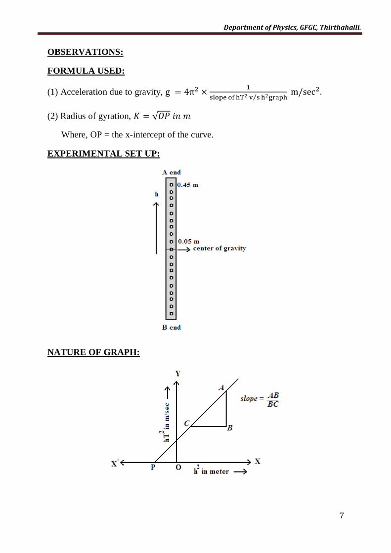
(1) Acceleration due to gravity,

⁄

(2) Radius of gyration, √

Where, OP = the x-intercept of the curve.


NATURE OF GRAPH:


8

TABULAR COLUMN:

Hole

no.

Distance

from C.G.

in m

Time for 20 oscillations in

seconds

Period

in sec

hT2 in

m /sec2

h2 in m

t1 t2

1

2

3

4

5

6

7

8

9

CALCULATIONS:


9

Expt. Name: SPIRAL SPRING

AIM: To determine the force constant and acceleration due to gravity using

spiral spring.

APPARATUS: Spiral spring, hanger, slotted weights, stop clock, meter scale,

stand, etc.

PROCEDURE: Hang a spiral spring from a rigid support as shown in figure

and attached a scale pan. With no load in the scale-pan, note down the zero

reading of the pointer on the scale. Place gently in the pan a load of, say 50 gm.

Now the spring slightly stretches and the pointer moves down on the scale. In

the steady position, note down the reading of the pointer. The difference of the

two readings is the extension of the spring for the load in the pan. Increase the

lead in the pan in equal steps until maximum permissible load is reached and

note down the corresponding pointer readings on the scale. The experiment is

repeated with decreasing loads.

A graph of extension v/s load is plotted. The slope of straight line is found.

Then force constant i.e., force per unit extension is calculated using the formula

K = 1 / slope.

Load the pan. Displace the pan vertically downward through a small distance

and release it. The spring performs simple harmonic oscillations. With the help

of a stop watch, note down the time of a number of oscillation (say 20 or 30).

Now divide the total time by the number of oscillations to find the time period

(time for one oscillation) T1. Increase the load in the pan to M2. As described

above, find the time period T2 for this load. Repeat the experiment with

different values of load.

Then acceleration due to gravity is calculated using the formula,

( )

(

)

RESULT:

(1) Force constant, K = ________ kg/m.



10

OBSERVATIONS:

FORMULA USED:

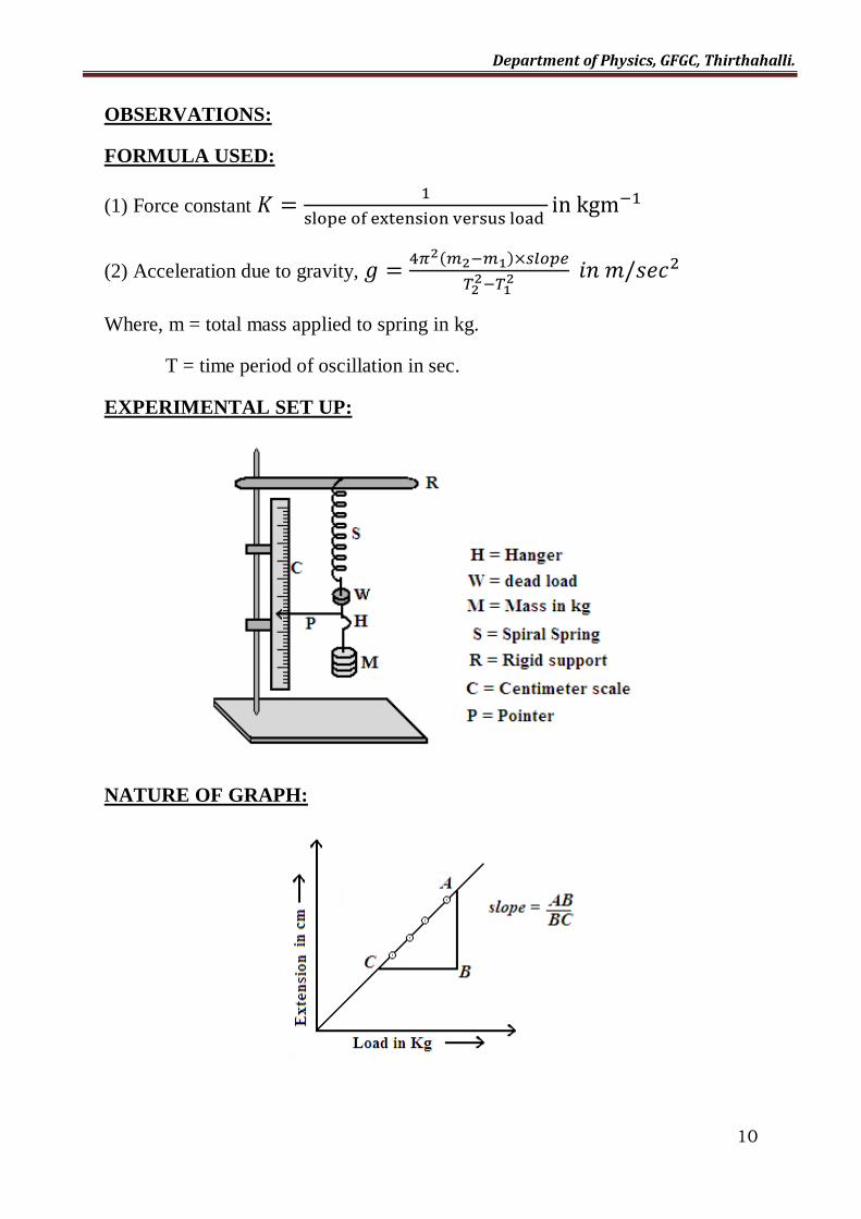
(1) Force constant

(2) Acceleration due to gravity, ( )

Where, m = total mass applied to spring in kg.

T = time period of oscillation in sec.


NATURE OF GRAPH:


11

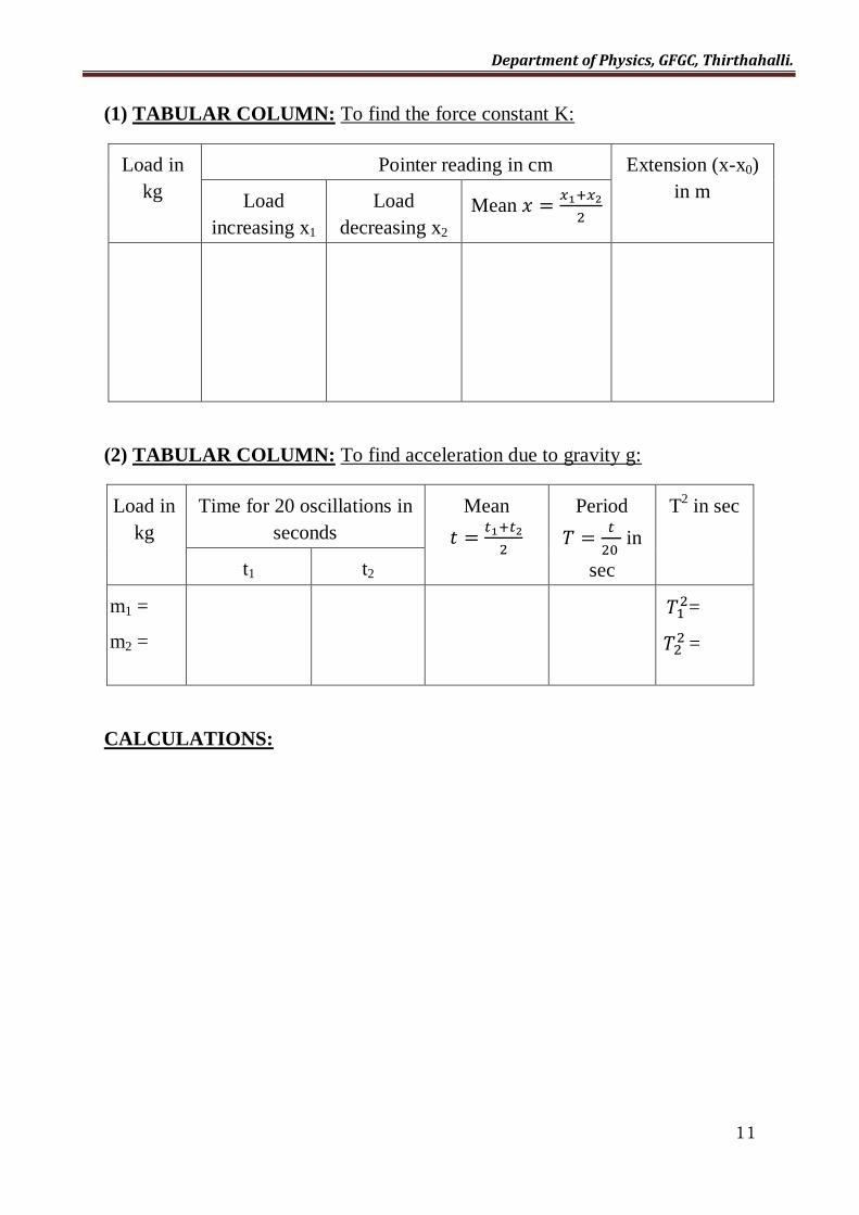
(1) TABULAR COLUMN: To find the force constant K:

Load in

kg

Pointer reading in cm Extension (x-x0)

in m Load

increasing x1

Load

decreasing x2 Mean

(2) TABULAR COLUMN: To find acceleration due to gravity g:

Load in

kg

Time for 20 oscillations in

seconds

Mean

Period

in

sec

T2 in sec

t1 t2

m1 =

m2 =

=

=

CALCULATIONS:


12

Expt. Name: STATIC TORSION

AIM: To determine the rigidity modulus η of the material of given rod by static

torsion.

APPARATUS: Static torsion apparatus, weight hanger, screw gauge.

PROCEDURE: In static torsion apparatus, one end of the experimental rod is

fixed firmly, the other end is fixed to a circular pulley. The free end of cord is

attached to a weight hanger. The twist between two points separated by a

distance ‘l’ can be measured by circular scale.

First, rod is brought into cyclic state. For this, the cord is round over the pulley

in clock wise direction. Weights are added to the hanger in steps of 0.5kg till

maximum convenient load is reached. The load is decreased in similar steps.

The cord is now round in anti-clockwise direction and the experiment is

repeated. In each case pointer reading is noted.

Experiment is repeated by decreasing the load. From the observations, twist ‘𝝓’

for load ‘m’ is calculated by the method of differences.

The length of the load ‘l’ from the fixed point to the pointer is measured. Using

a screw gauge, the diameter of the rod is measured and radius ‘r’ is calculated.

The radius ‘R’ of the pulley is determined by finding its circumference using a

thread.

A graph of load v/s twist is plotted. The slope of straight line is found. Using the

formula rigidity modulus is calculated.

RESULT: Rigidity modulus of the material of the rod, η = ________ N/m2.


13

OBSERVATIONS:

FORMULA USED: Rigidity modulus of the material of the road,

⁄

Where, g = acceleration due to gravity in m/sec2.

R = radius of pulley in m.

L = Distance between fixed end and the pointer = ________ m.

r = radius of the rod in m.


NATURE OF GRAPH:

To find Radius of pulley:

Circumference of the pulley, C = ______ cm.

We know that, C = 2πR and R=2π/C = ------- =__________ m


14

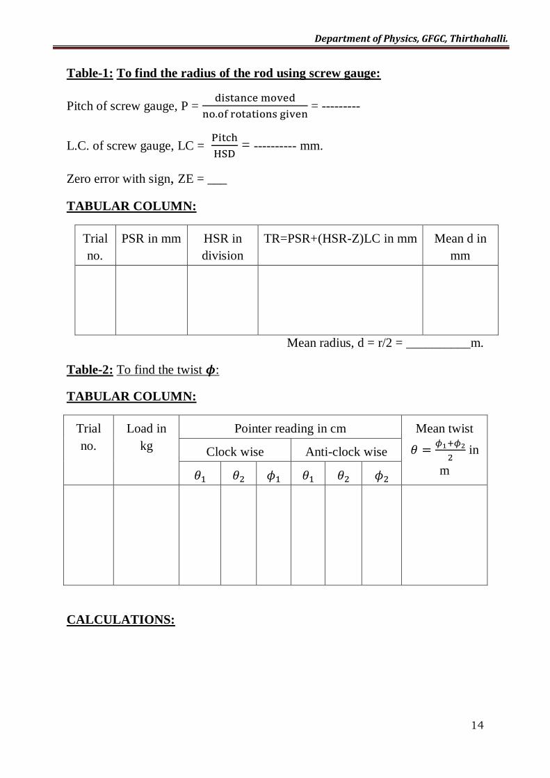
Table-1: To find the radius of the rod using screw gauge:

Pitch of screw gauge, P =

= ---------

L.C. of screw gauge, LC =

= ---------- mm.

Zero error with sign, ZE = ___

TABULAR COLUMN:

Trial

no.

PSR in mm HSR in

division

TR=PSR+(HSR-Z)LC in mm Mean d in

mm

Mean radius, d = r/2 = __________m.

Table-2: To find the twist 𝝓:

TABULAR COLUMN:

Trial

no.

Load in

kg

Pointer reading in cm Mean twist

in

m

Clock wise Anti-clock wise

CALCULATIONS:


15

Expt. Name: YOUNG’S MODULUS BY STRETCHING

AIM: To determine young’s modulus (q) of the material of the thin wire by

stretching.

APPARATUS: scale and screw gauge, stretching apparatus, weight hanger, etc.

PROCEDURE: Using a screw gauge, the diameter of the experimental wire is

measured for 3 trails and its average radius ‘r’ is calculated.

The experimental wire is brought into cyclic shape by loading it in equal steps

of 0.5kg up to a maximum by 2.5kg and unloaded in equal steps. This is

repeated to 3 to 4 times. The reading on the screw scale is noted.

Weights are added to the hanger in equal steps by 0.5kg to a maximum of 2.5kg

and in each case readings are noted. The load is then decreased in similar steps

and in each step the reading is noted.

In each observation, the average screw reading for each load is calculated. The

extension (l) of the wire for mass (m) is determined by the method of

differences.

A graph of load versus extension is plotted. The slope of the straight line is

measured.

The young’s modulus of the wire is calculated using the equation,

RESULT: Young’s modulus of material of wire, η = __________Nm-2

.


16

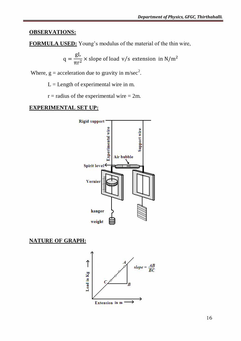
OBSERVATIONS:

FORMULA USED: Young’s modulus of the material of the thin wire,

⁄


L = Length of experimental wire in m.

r = radius of the experimental wire = 2m.


NATURE OF GRAPH:


17

Table-1: To find the radius of the wire using screw gauge:


= ---------


= ---------- mm.


TABULAR COLUMN:

Trial

no.

PSR in mm HSR TR=PSR+(HSR-Z)LC in mm Mean d in

mm

Mean radius, d = r/2 = __________m.

Table-2: To find the extension of wire:

Least Count =

= ----------mm.

TABULAR COLUMN:

Load in

kg

Reading in mm Extension (x-x0)

in m Load

increasing x1

Load

decreasing x2 Mean

x0=

CALCULATIONS


18

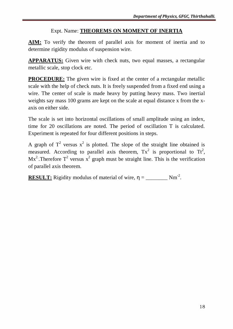
Expt. Name: THEOREMS ON MOMENT OF INERTIA

AIM: To verify the theorem of parallel axis for moment of inertia and to

determine rigidity modulus of suspension wire.

APPARATUS: Given wire with check nuts, two equal masses, a rectangular

metallic scale, stop clock etc.

PROCEDURE: The given wire is fixed at the center of a rectangular metallic

scale with the help of check nuts. It is freely suspended from a fixed end using a

wire. The center of scale is made heavy by putting heavy mass. Two inertial

weights say mass 100 grams are kept on the scale at equal distance x from the x-

axis on either side.

The scale is set into horizontal oscillations of small amplitude using an index,

time for 20 oscillations are noted. The period of oscillation T is calculated.

Experiment is repeated for four different positions in steps.

A graph of T2 versus x

2 is plotted. The slope of the straight line obtained is

measured. According to parallel axis theorem, Tx2 is proportional to Tt

2,

Mx2..Therefore T

2 versus x

2 graph must be straight line. This is the verification

of parallel axis theorem.

RESULT: Rigidity modulus of material of wire, η = ________ Nm-2

.


19

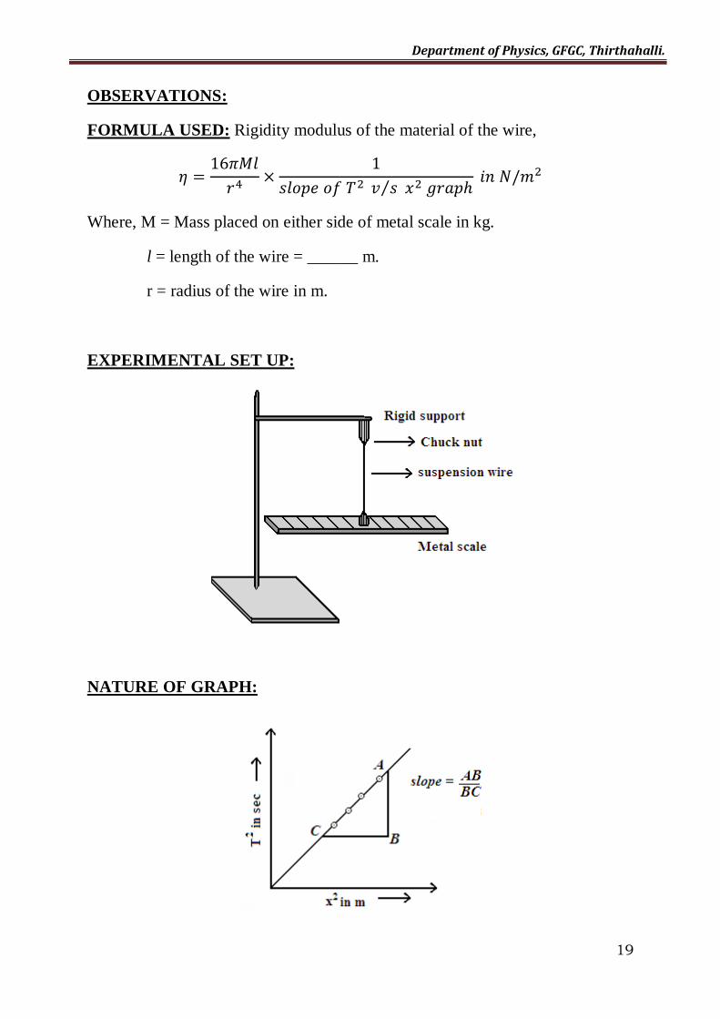
OBSERVATIONS:

FORMULA USED: Rigidity modulus of the material of the wire,

⁄

Where, M = Mass placed on either side of metal scale in kg.

l = length of the wire = ______ m.

r = radius of the wire in m.


NATURE OF GRAPH:


20

Table-1: To find the radius of the wire using screw gauge:


= ---------


= ----------mm.


TABULAR COLUMN:

Trial

no.

PSR in mm HSR in

division

TR=PSR+(HSR-Z)LC in mm Mean d in

mm

Mean radius, d = r/2 = __________m.

Table-2: To find the time period T:

Trial

no.

Distance x

in m

Time for 20 oscillations in sec Period

in

sec

x2 in

m2

T2 in sec

2

t1 t2

CALCULATIONS:


21

Expt. Name: FLY WHEEL

AIM: To determine moment of inertia of a flywheel about its axis of rotation

and hence to calculate its mass.

APPARATUS: Fly wheel, stop clock, weight hanger, slotted weights, etc.

PROCEDURE: Using a vernier calipers the average radius ‘r’ of the axle is

determined. Using a thread, the circumference C of the wheel is measured. Its

radius is calculated using the formula R = C/2π.

A thread is fixed to the peg in the axel and is wound round the axel for a few

turns without overwrapping. To the other end, a weight hanger is attached. A

mark is made on the wheel and is held such that, the index coincides with the

mark.

A load ‘m’ in kg is placed in the hanger without any initial jerk, the wheel is

allowed to rotate. Simultaneously a stop clock is started. The time t for 10

revolutions before the load reaches the ground is noted. The experiment is

repeated for 3 trials and average time for n revolutions is noted. The angular

acceleration α is calculated using the formula,

Experiment is repeated for different loads. Observations are tabulated as shown.

A graph of angular acceleration versus mass is plotted. The slope of the straight

line is calculated. The moment of inertia of the fly wheel about the axis of

rotation is calculated using the formula,

The mass ‘m’ is calculated using the formula

RESULT:

(1) Moment of inertia of flywheel, I = _______ kgm2.

(2) Mass of flywheel, M = _______ kg.


22

OBSERVATIONS:

FORMULA USED:

(1) The moment of inertia of the fly wheel,

(2) The mass of the fly wheel,


r = radius of the axel in m.

R = Radius of the wheel in m.


NATURE OF GRAPH:

To find Radius of wheel:

Circumference of the wheel, C = ______ cm.

We know that, C = 2πR and R=2π/C = ------- =__________ m


23

Table-1: To find the radius of the axel using vernier calipers:

L.C. of vernier calipers, LC =

= ---------- cm.

TABULAR COLUMN:

Trial

no.

MSR in cm CVD TR=MSR+(CVD)LC in cm Mean d in

cm

Mean radius, d = r/2 = __________m.

Table-2: To find the angular acceleration:

Trial

no.

Mass attached

to thread m in

kg

Time for ‘n’ rotations in sec t2 in

sec

in

rad/sec2

t1 t2

CALCULATIONS:


24

Expt. Name: STEFAN - BOLTZMANN LAW

AIM: To determine the radiation index ‘n’ by using log I versus log R graph.

APPARATUS: Meter Bridge, Galvanometer, Resistance box, Rheostat, etc.

PROCEDURE: The connections are made as shown in the circuit diagram.

Suitable resistance S in resistance box is kept constant. The current in the

miliammeter is adjusted by using a rheostat and the corresponding balancing

length ‘l’ is measured using sliding contact and also the value (1-l) is

determined.

Finally calculate the resistance ‘R’ of the filament and is calculated using the

formula,

where S is the constant value of resistance.

The experiment is repeated for 3 trials. In each case the length l and R are

determined. The values of log C and log R are calculated. A graph of log I vs

log R is drawn. The slope of straight line is measured. Using the value of slope,

we can calculate the radiation index ‘n’ by the formula n = (2m+1) where m is

the slope.

RESULT: Radiation index, n = ________

Stefan Boltzmann law is verified.


25

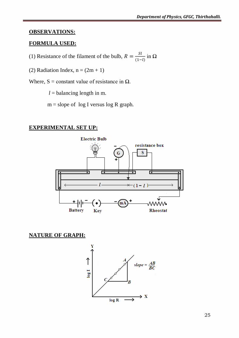
OBSERVATIONS:

FORMULA USED:

(1) Resistance of the filament of the bulb,

( ) in Ω

(2) Radiation Index, n = (2m + 1)

Where, S = constant value of resistance in Ω.

l = balancing length in m.

m = slope of log I versus log R graph.


NATURE OF GRAPH:


26

TABULAR COLUMN:

Trial

no.

S in

Ω

Current

I in mA

Balancing

length l in m

(1-l)

in m

( )

in Ω

log R log I

CALCULATIONS:

physics laboratory manual i b.sc., i semester …

Documents