physics 523, general relativity homework 1jbourj/gr/homeworks.pdf · physics 523, general...
TRANSCRIPT
Physics , General RelativityHomework
Due Wednesday, th September
Jacob Lewis Bourjaily
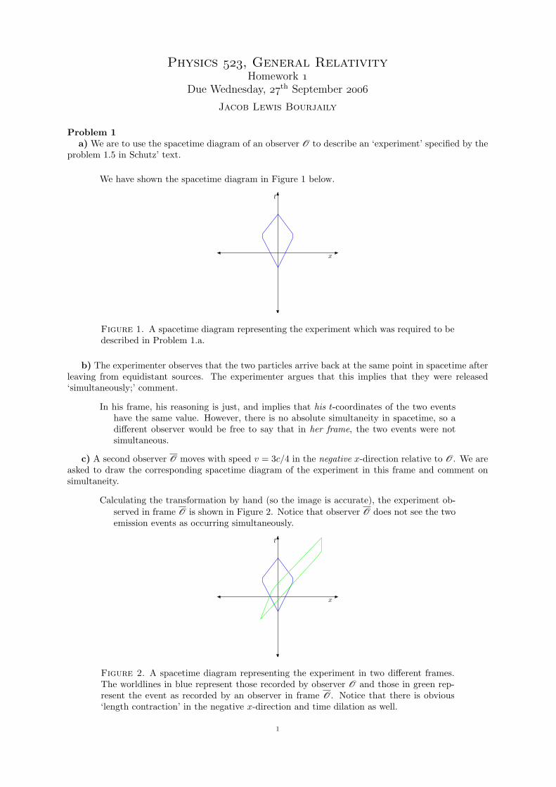
Problem 1a) We are to use the spacetime diagram of an observer O to describe an ‘experiment’ specified by the
problem 1.5 in Schutz’ text.
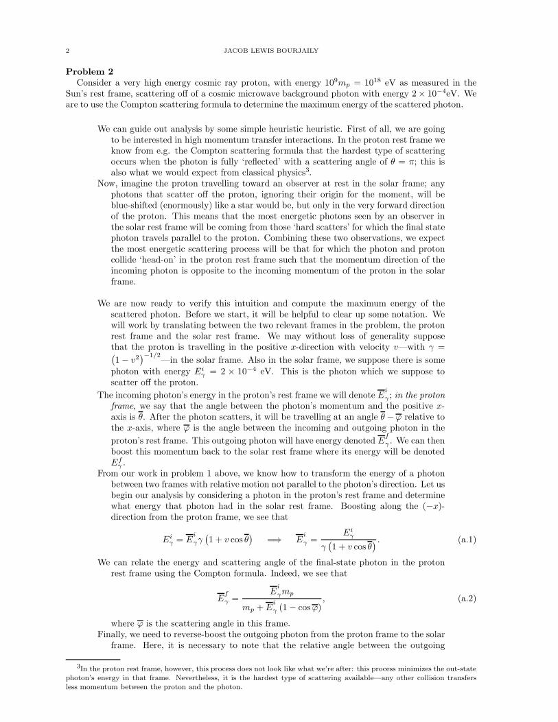
We have shown the spacetime diagram in Figure 1 below.
t
x
Figure 1. A spacetime diagram representing the experiment which was required to bedescribed in Problem 1.a.
b) The experimenter observes that the two particles arrive back at the same point in spacetime afterleaving from equidistant sources. The experimenter argues that this implies that they were released‘simultaneously;’ comment.
In his frame, his reasoning is just, and implies that his t-coordinates of the two eventshave the same value. However, there is no absolute simultaneity in spacetime, so adifferent observer would be free to say that in her frame, the two events were notsimultaneous.
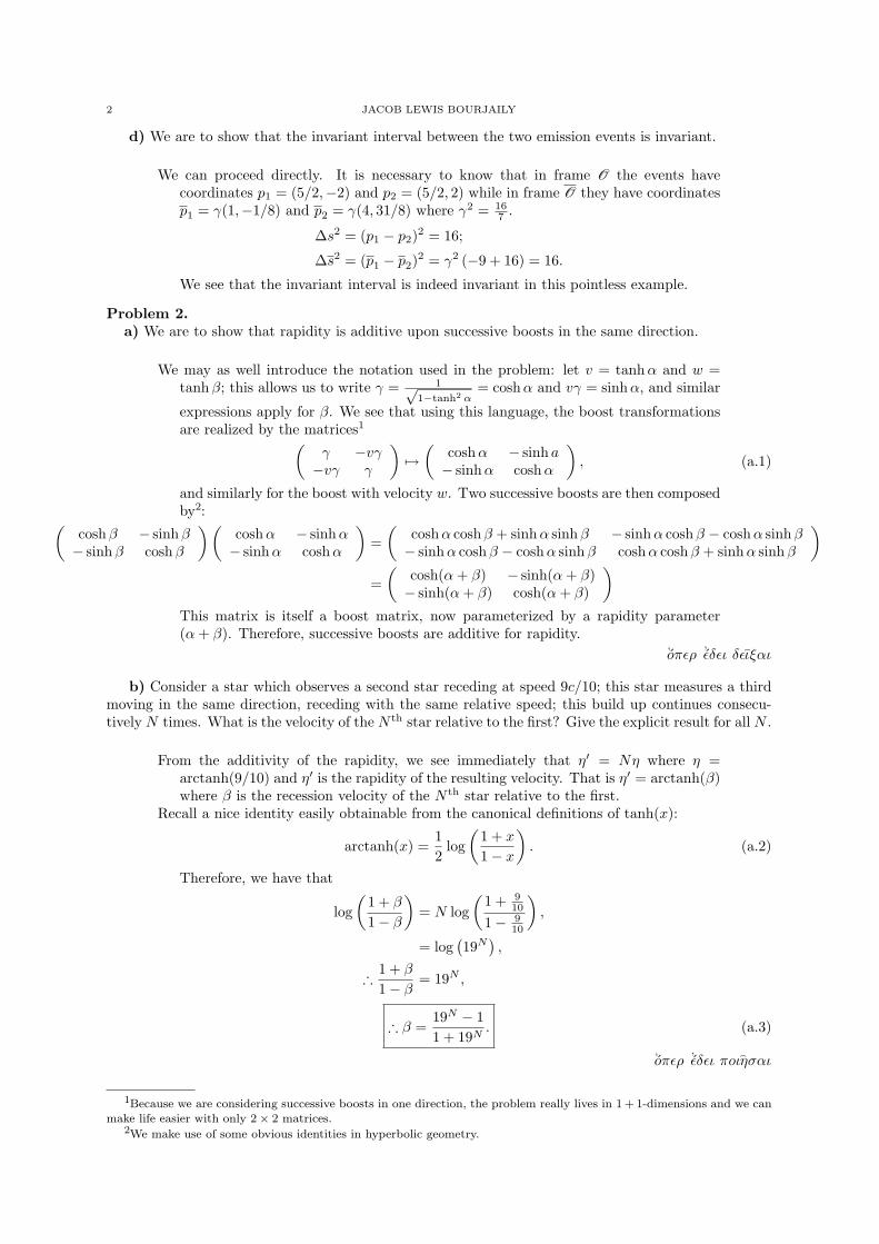
c) A second observer O moves with speed v = 3c/4 in the negative x-direction relative to O. We areasked to draw the corresponding spacetime diagram of the experiment in this frame and comment onsimultaneity.
Calculating the transformation by hand (so the image is accurate), the experiment ob-served in frame O is shown in Figure 2. Notice that observer O does not see the twoemission events as occurring simultaneously.
t
x
Figure 2. A spacetime diagram representing the experiment in two different frames.The worldlines in blue represent those recorded by observer O and those in green rep-resent the event as recorded by an observer in frame O. Notice that there is obvious‘length contraction’ in the negative x-direction and time dilation as well.
1
2 JACOB LEWIS BOURJAILY
d) We are to show that the invariant interval between the two emission events is invariant.
We can proceed directly. It is necessary to know that in frame O the events havecoordinates p1 = (5/2,−2) and p2 = (5/2, 2) while in frame O they have coordinatesp1 = γ(1,−1/8) and p2 = γ(4, 31/8) where γ2 = 16
7 .
∆s2 = (p1 − p2)2 = 16;
∆s2 = (p1 − p2)2 = γ2 (−9 + 16) = 16.
We see that the invariant interval is indeed invariant in this pointless example.
Problem 2.a) We are to show that rapidity is additive upon successive boosts in the same direction.
We may as well introduce the notation used in the problem: let v = tanh α and w =tanh β; this allows us to write γ = 1√
1−tanh2 α= cosh α and vγ = sinh α, and similar
expressions apply for β. We see that using this language, the boost transformationsare realized by the matrices1(
γ −vγ−vγ γ
)7→
(cosh α − sinh a− sinhα cosh α
), (a.1)
and similarly for the boost with velocity w. Two successive boosts are then composedby2:(
cosh β − sinhβ− sinh β coshβ
)(coshα − sinhα− sinhα cosh α
)=
(coshα cosh β + sinh α sinhβ − sinhα cosh β − cosh α sinhβ− sinhα cosh β − cosh α sinhβ cosh α coshβ + sinh α sinhβ
)
=(
cosh(α + β) − sinh(α + β)− sinh(α + β) cosh(α + β)
)
This matrix is itself a boost matrix, now parameterized by a rapidity parameter(α + β). Therefore, successive boosts are additive for rapidity.
‘oπερ ’εδει δειξαι
b) Consider a star which observes a second star receding at speed 9c/10; this star measures a thirdmoving in the same direction, receding with the same relative speed; this build up continues consecu-tively N times. What is the velocity of the N th star relative to the first? Give the explicit result for all N .
From the additivity of the rapidity, we see immediately that η′ = Nη where η =arctanh(9/10) and η′ is the rapidity of the resulting velocity. That is η′ = arctanh(β)where β is the recession velocity of the N th star relative to the first.
Recall a nice identity easily obtainable from the canonical definitions of tanh(x):
arctanh(x) =12
log(
1 + x
1− x
). (a.2)
Therefore, we have that
log(
1 + β
1− β
)= N log
(1 + 9
10
1− 910
),
= log(19N
),
∴ 1 + β
1− β= 19N ,
∴ β =19N − 11 + 19N
. (a.3)
‘oπερ ’εδει πoιησαι
1Because we are considering successive boosts in one direction, the problem really lives in 1 + 1-dimensions and we canmake life easier with only 2× 2 matrices.
2We make use of some obvious identities in hyperbolic geometry.
PHYSICS : GENERAL RELATIVITY HOMEWORK 3
Problem 3.a) Consider a boost in the x-direction with speed vA = tanh α followed by a boost in the y-direction
with speed vB = tanh β. We are to show that the resulting Lorentz transformation can be written as apure rotation followed by a pure boost and determine the rotation and boost.
This is a 2 + 1-dimensional problem—the entire problem involves only the SO(2, 1)subgroup of the Lorentz group. Now, although there must certainly be easy ways ofsolving this problem without setting up a system of equations and using trigonometricidentities, we will stick with the obvious answer/easy math route—indeed, the algebrais not that daunting and the equations are easily solved.
The brute-force technique involves writing out the general matrices for both operationsand (consistently) matching terms. The two successive boosts result in
coshβ 0 − sinhβ
0 1 0− sinhβ 0 cosh β
cosh α − sinhβ 0− sinhα coshβ 0
0 0 1
=
cosh α cosh β − sinh α cosh β − sinhβ− sinh α cosh α 0
− cosh α sinhβ sinh α sinh β cosh β
(a.4)And a rotation about z through the angle θ followed by a boost in the (cos λ, sinλ)-
direction with rapidity η is given by3
cosh η − sinh η cosλ − sinh η sin λ− sinh η cos λ 1 + cos2 λ(cosh η − 1) cos λ sin λ(cosh η − 1)− sinh η sinλ cosλ sin λ(cosh η − 1) 1 + sin2 λ(cosh η − 1)
1 0 00 cos θ − sin θ0 sin θ cos θ
=
cosh η − sinh η (cos λ cos θ + sin λ sin θ) − sinh η (sin λ cos θ − cosλ sin θ)− sinh η cosλ cos θ + (cosh η − 1)(cos2 λ cos θ + cosλ sin λ sin θ) − sin θ + (cosh η − 1)(cos λ sinλ cos θ − cos2 λ sin θ)− sinh η sin λ sin θ + (cosh η − 1)(sin2 λ sin θ + cos λ sin λ cos θ) cos θ + (cosh η − 1)(sin2 λ cos θ − cos λ sin λ sin θ)
The system is over-constrained, and it is not hard to find the solutions. For example,the (00)-entry in both transformation matrices must match,
∴ cosh η = coshα cosh α. (a.5)
Looking at the (10) and (20) entries in each box, we see that
sinh η cosλ = sinh α;sin η sin λ = cosh α sinhβ;
which together imply
∴ tan λ =sinhβ
tanh α. (a.6)
Lastly, we must find θ; this can be achieved via the equation matching for the (12)entry:
sin θ = (cosh η − 1)(cosλ sin λ cos θ − cos2 λ sin θ
);
=⇒ tan θ(1 + cos2 λ (cosh η − 1)
)= (cosh η − 1) cos λ sin λ,
∴ tan θ =(cosh η − 1) cos λ sinλ
1 + cos2 λ cosh η − cos2 λ. (a.7)
b) A spaceship A moves with velocity vA along x relative to O and another, B, moves with speedvB along y relative to A. Determine the direction and velocity of the frame O relative to B.
To map this exactly to the previous problem, we do things backwards and transformB → A followed by A → O relative to B. That is, let tanh α = −vB and tanh β = vA.Now, the magnitude of the velocity of frame O relative to B has rapidity given byequation (a.5), and is moving in the direction an angle π−(θ+λ) relative to A whereλ and θ are given by equations (a.6) and (a.7), respectively.
3This required a bit of algebra, but it isn’t worth doing in public.

Physics , General RelativityHomework
Due Monday, th October
Jacob Lewis Bourjaily
Problem 1Let frame O move with speed v in the x-direction relative to frame O. A photon with frequency ν
measured in O moves at an angle θ relative to the x-axis.a) We are to determine the frequency of the photon in O’s frame.
From the set up we know that the momentum of the photon in O is1 (E, E cos θ, E sin θ)—that this momentum is null is manifest. The energy of the photon is of course E = hνwhere h is Planck’s constant and ν is the frequency in O’s frame.
Using the canonical Lorentz boost equation, the energy measured in frame O is given by
E = Eγ − E cos θvγ,
= hνγ − hν cos θvγ.
But E = hν, so we see
∴
ν
ν= γ (1− v cos θ) . (a.1)
‘oπǫρ ’ǫδǫι πoιησαι
b) We are to find the angle θ at which there is no Doppler shift observed.
All we need to do is find when ν/ν = 1 = γ (1− v cos θ). Every five-year-old shouldbe able to invert this to find that the angle at which no Doppler shift is observed isgiven by
∴ cos θ =1
v
(1−
√1− v2
). (b.1)
Notice that this implies that an observer moving close to the speed of light relativeto the cosmic microwave background2 will see a narrow ‘tunnel’ ahead of highly blue-shifted photons and large red-shifting outside this tunnel. As the relative velocityincreases, the ‘tunnel’ of blue-shifted photons gets narrower and narrower.
c) We are asked to compute the result in part a above using the technique used above.
This was completed already. We made use of Schutz’s equation (2.35) when we wrotethe four-momentum of the photon in a manifestly light-like form, and we made useof Schutz’s equation (2.38) when used the fact that E = hν.
1We have aligned the axes so that the photon is travelling in the xy-plane. This is clearly a choice we are free to make.2The rest frame of the CMB is defined to be that for which the CMB is mostly isotropic—specifically, the relative
velocity at which no dipole mode is observed in the CMB power spectrum.
1
2 JACOB LEWIS BOURJAILY
Problem 2Consider a very high energy cosmic ray proton, with energy 109mp = 1018 eV as measured in the
Sun’s rest frame, scattering off of a cosmic microwave background photon with energy 2× 10⁻⁴eV. Weare to use the Compton scattering formula to determine the maximum energy of the scattered photon.
We can guide out analysis by some simple heuristic heuristic. First of all, we are goingto be interested in high momentum transfer interactions. In the proton rest frame weknow from e.g. the Compton scattering formula that the hardest type of scatteringoccurs when the photon is fully ‘reflected’ with a scattering angle of θ = π; this isalso what we would expect from classical physics3.
Now, imagine the proton travelling toward an observer at rest in the solar frame; anyphotons that scatter off the proton, ignoring their origin for the moment, will beblue-shifted (enormously) like a star would be, but only in the very forward directionof the proton. This means that the most energetic photons seen by an observer inthe solar rest frame will be coming from those ‘hard scatters’ for which the final statephoton travels parallel to the proton. Combining these two observations, we expectthe most energetic scattering process will be that for which the photon and protoncollide ‘head-on’ in the proton rest frame such that the momentum direction of theincoming photon is opposite to the incoming momentum of the proton in the solarframe.
We are now ready to verify this intuition and compute the maximum energy of thescattered photon. Before we start, it will be helpful to clear up some notation. Wewill work by translating between the two relevant frames in the problem, the protonrest frame and the solar rest frame. We may without loss of generality supposethat the proton is travelling in the positive x-direction with velocity v—with γ =(1− v2
)−1/2
—in the solar frame. Also in the solar frame, we suppose there is some
photon with energy Eiγ = 2 × 10⁻⁴ eV. This is the photon which we suppose to
scatter off the proton.
The incoming photon’s energy in the proton’s rest frame we will denote Ei
γ ; in the proton
frame, we say that the angle between the photon’s momentum and the positive x-axis is θ. After the photon scatters, it will be travelling at an angle θ−ϕ relative tothe x-axis, where ϕ is the angle between the incoming and outgoing photon in the
proton’s rest frame. This outgoing photon will have energy denoted Ef
γ . We can thenboost this momentum back to the solar rest frame where its energy will be denotedEf
γ .From our work in problem 1 above, we know how to transform the energy of a photon
between two frames with relative motion not parallel to the photon’s direction. Let usbegin our analysis by considering a photon in the proton’s rest frame and determinewhat energy that photon had in the solar rest frame. Boosting along the (−x)-direction from the proton frame, we see that
Eiγ = E
i
γγ(1 + v cos θ
)=⇒ E
i
γ =Ei
γ
γ(1 + v cos θ
) . (a.1)
We can relate the energy and scattering angle of the final-state photon in the protonrest frame using the Compton formula. Indeed, we see that
Ef
γ =E
i
γmp
mp + Ei
γ (1− cosϕ), (a.2)
where ϕ is the scattering angle in this frame.Finally, we need to reverse-boost the outgoing photon from the proton frame to the solar
frame. Here, it is necessary to note that the relative angle between the outgoing
3In the proton rest frame, however, this process does not look like what we’re after: this process minimizes the out-statephoton’s energy in that frame. Nevertheless, it is the hardest type of scattering available—any other collision transfersless momentum between the proton and the photon.
PHYSICS : GENERAL RELATIVITY HOMEWORK 3
202
2
0
2
20
10
0
10
Log E f eV
02
2
0
2
202
2
0
2
0
0.0005
0.001
0.0015
E f eV
02
2
0
2
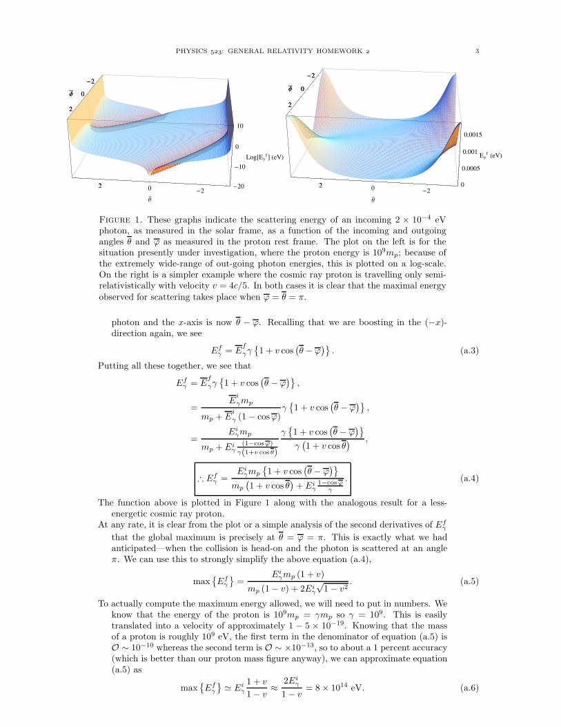
Figure 1. These graphs indicate the scattering energy of an incoming 2 × 10⁻⁴ eVphoton, as measured in the solar frame, as a function of the incoming and outgoingangles θ and ϕ as measured in the proton rest frame. The plot on the left is for thesituation presently under investigation, where the proton energy is 109mp; because ofthe extremely wide-range of out-going photon energies, this is plotted on a log-scale.On the right is a simpler example where the cosmic ray proton is travelling only semi-relativistically with velocity v = 4c/5. In both cases it is clear that the maximal energy
observed for scattering takes place when ϕ = θ = π.
photon and the x-axis is now θ − ϕ. Recalling that we are boosting in the (−x)-direction again, we see
Efγ = E
f
γγ1 + v cos
(θ − ϕ
). (a.3)
Putting all these together, we see that
Efγ = E
f
γγ1 + v cos
(θ − ϕ
),
=E
i
γmp
mp + Ei
γ (1− cosϕ)γ
1 + v cos
(θ − ϕ
),
=Ei
γmp
mp + Eiγ
(1−cos ϕ)
γ(1+v cos θ)
γ1 + v cos
(θ − ϕ
)
γ(1 + v cos θ
) ,
∴ Efγ =
Eiγmp
1 + v cos
(θ − ϕ
)
mp
(1 + v cos θ
)+ Ei
γ1−cos ϕ
γ
. (a.4)
The function above is plotted in Figure 1 along with the analogous result for a less-energetic cosmic ray proton.
At any rate, it is clear from the plot or a simple analysis of the second derivatives of Efγ
that the global maximum is precisely at θ = ϕ = π. This is exactly what we hadanticipated—when the collision is head-on and the photon is scattered at an angleπ. We can use this to strongly simplify the above equation (a.4),
maxEf
γ
=
Eiγmp (1 + v)
mp (1− v) + 2Eiγ
√1− v2
. (a.5)
To actually compute the maximum energy allowed, we will need to put in numbers. Weknow that the energy of the proton is 109mp = γmp so γ = 109. This is easilytranslated into a velocity of approximately 1 − 5 × 10⁻¹⁹. Knowing that the massof a proton is roughly 109 eV, the first term in the denominator of equation (a.5) isO ∼ 10−10 whereas the second term is O ∼ ×10−13, so to about a 1 percent accuracy(which is better than our proton mass figure anyway), we can approximate equation(a.5) as
maxEf
γ
≃ Ei
γ
1 + v
1− v≈
2Eiγ
1− v= 8× 10¹⁴ eV. (a.6)
4 JACOB LEWIS BOURJAILY
Therefore, the maximum energy of a scattered CMB photon from a 1018 eV cosmic rayproton is about 400 TeV—much higher than collider-scale physics. However, therate of these types of hard-scatters is enormously low. Indeed, recalling the pictureof a narrowing tunnel of blue-shift at high boost, we can use our work from problem1 to see that only photons within a 0.0025 cone about the direction of motion ofthe proton are blue-shifted at all—and these are the only ones that can gain anymeaningful energy from the collision. This amounts to a phase-space suppressionof around 10−10 even before we start looking at the small rate and low densitiesinvolved.
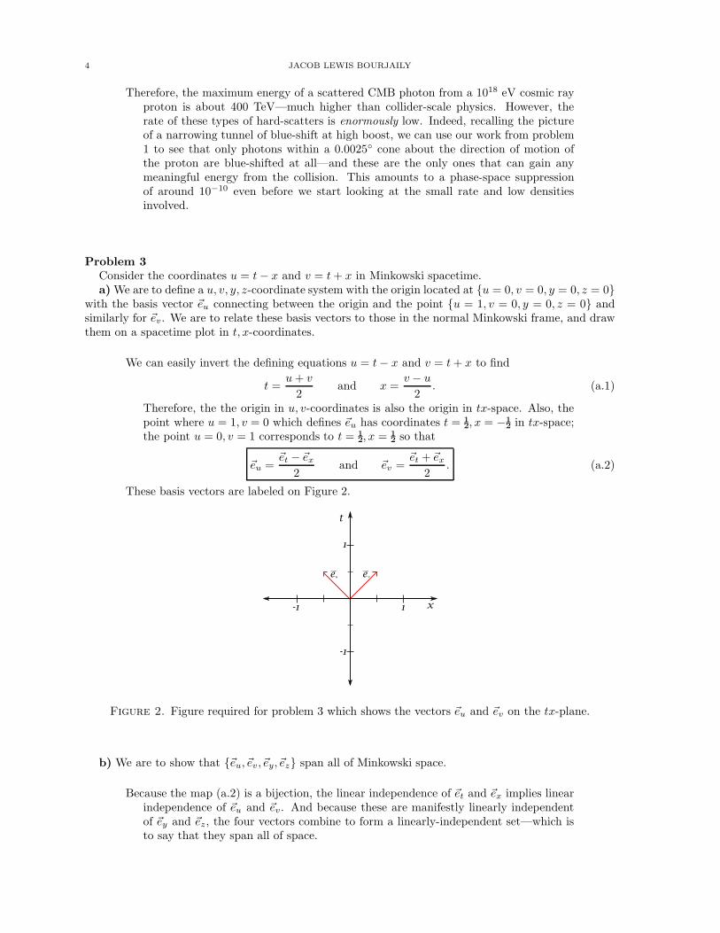
Problem 3Consider the coordinates u = t− x and v = t + x in Minkowski spacetime.a) We are to define a u, v, y, z-coordinate system with the origin located at u = 0, v = 0, y = 0, z = 0
with the basis vector ~eu connecting between the origin and the point u = 1, v = 0, y = 0, z = 0 andsimilarly for ~ev. We are to relate these basis vectors to those in the normal Minkowski frame, and drawthem on a spacetime plot in t, x-coordinates.
We can easily invert the defining equations u = t− x and v = t + x to find
t =u + v
2and x =
v − u
2. (a.1)
Therefore, the the origin in u, v-coordinates is also the origin in tx-space. Also, thepoint where u = 1, v = 0 which defines ~eu has coordinates t = ½, x = −½ in tx-space;the point u = 0, v = 1 corresponds to t = ½, x = ½ so that
~eu =~et − ~ex
2and ~ev =
~et + ~ex
2. (a.2)
These basis vectors are labeled on Figure 2.
Figure 2. Figure required for problem 3 which shows the vectors ~eu and ~ev on the tx-plane.
b) We are to show that ~eu, ~ev, ~ey, ~ez span all of Minkowski space.
Because the map (a.2) is a bijection, the linear independence of ~et and ~ex implies linearindependence of ~eu and ~ev. And because these are manifestly linearly independentof ~ey and ~ez, the four vectors combine to form a linearly-independent set—which isto say that they span all of space.
PHYSICS : GENERAL RELATIVITY HOMEWORK 5
c) We are to find the components of the metric tensor in this basis.
The components of the metric tensor in any basis ~ei is given by the matrix gij =g (~ei, ~ej) where g (·, ·) is the metric on spacetime. Because we have equation (a.2)which relates ~eu and ~ev to the tx-bases, we can compute all the relevant inner productsusing the canonical Minkowski metric. Indeed we find,
gij =
0 1/2 0 01/2 0 0 00 0 1 00 0 0 1
. (c.1)
d) We are to show that ~eu and ~ev are null but they are not orthogonal.
In part c above we needed to compute the inner products of all the basis vectors, includ-ing ~eu and ~ev. There we found that g (~eu, ~ev) = 1/2, so ~eu and ~ev are not orthogonal.However, g (~eu, ~eu) = g (~eu, ~ev) = 0, so they are both null.
e) We are to compute the one-forms du, dv, g(~eu, ·), and g(~ev, ·).
As scalar functions on spacetime, it is easy to compute the exterior derivatives of u andv. Indeed, using their respective definitions, we find immediately that
du = dt− dx and dv = dt + dx. (e.1)
The only difference that arises when computing g(~eu, ·), for example, is that the com-
ponents of ~eu are given in terms of the basis vectors ~et and ~ex as in equation (a.2).Therefore in the usual Minkowski component notation, we have ~eu = (½,−½, 0, 0) and~ev = (½, ½, 0, 0) . Using our standard Minkowski metric we see that
g (~eu, ·) = −1
2dt− 1
2dx and g (~ev, ·) = −1
2dt +
1
2dx. (e.2)
Problem 4We are to give an example of four linearly independent null vectors in Minkowski space and show why
it is not possible to make them all mutually orthogonal.
An easy example that comes to mind uses the coordinates x−, x+, y+, z+ given by
x− = t− x x+ = t+ = x y+ = t + y z+ = t + z. (a.1)
In case it is desirable to be condescendingly specific, this corresponds to taking basisvectors ~ex−, ~ex+, ~ey+, ~ez+ where
~ex− =~et − ~ex
2~ex+ =
~et + ~ex
2~ey+ =
~et + ~ey
2~ez+ =
~et + ~ez
2. (a.2)
It is quite obvious that each of these vectors is null, and because they are related to theoriginal basis by an invertible map they still span the space. Again, to be specific4,notice that ~et = ~ex−+~ex+ and so we may invert the other expressions by ~ei = 2~ei+−~et
where i = x, y, z.Let us now show that four linearly independent, null vectors cannot be simultaneously
mutually orthogonal. We proceed via reductio ad absurdum: suppose that the set~vii=1,...4 were such linearly independent, mutually orthogonal and null. Becausethey are linearly independent, they can be used to define a basis which has an asso-ciated metric, say g. Now, as a matrix the entries of g are given by gij = g (~vi, ~vj);because all the vectors are assumed to be orthogonal and null, all the entries of g are
4Do you, ye grader, actually care for me to be this annoyingly specific?
6 JACOB LEWIS BOURJAILY
zero. This means that it has zero positive eigenvalues and zero negative eigenvalues—which implies signature(g) = 0. But the signature of Minkowski spacetime must be±2 5, and this is basis-independent. −→←−
To go one step further, the above argument actually implies that no null vector can besimultaneously orthogonal to and linearly independent of any three vectors.
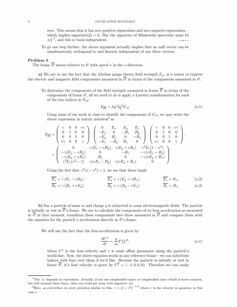
Problem 5The frame O moves relative to O with speed v in the z-direction.
a) We are to use the fact that the Abelian gauge theory field strength Fµν is a tensor to express
the electric and magnetic field components measured in O in terms of the components measured in O.
To determine the components of the field strength measured in frame O in terms of thecomponents of frame O, all we need to do is apply a Lorentz transformation for eachof the two indices in Fab:
Fab = Λ ca Λ d
bFcd. (a.1)
Using some of our work in class to identify the components of Fcd, we may write theabove expression in matrix notation6 as
Fab =
γ 0 0 vγ0 1 0 00 0 1 0vγ 0 0 γ
·
0 Ex Ey Ez
−Ex 0 −Bz By
−Ey Bz 0 −Bx
−Ez −By Bx 0
·
γ 0 0 vγ0 1 0 00 0 1 0vγ 0 0 γ
,
=
0 γ(Ex − vBy) γ(Ey + vBx) γ2Ez(1− v2)−γ(Ex − vBy) 0 −Bz −γ(vEx −By)−γ(Ey + vBx) Bz 0 −γ(vEy + Bx)γ2Ez(v
2 − 1) γ(vEx −By) γ(vEy + Bx) 0
.
Using the fact that γ2(1− v2) = 1, we see that these imply
Ex = γ (Ex − vBy) Ey = γ (Ey + vBx) Ez = Ez , (a.2)
Bx = γ (Bx + vEy) By = γ (By − vEx) Bz = Bz. (a.3)
b) Say a particle of mass m and charge q is subjected to some electromagnetic fields. The particleis initially at rest in O’s frame. We are to calculate the components of its four-acceleration as measuredin O at that moment, transform these components into those measured in O and compare them withthe equation for the particle’s acceleration directly in O’s frame.
We will use the fact that the four-acceleration is given by
dUa
dτ=
q
mF a
bUb, (a.1)
where Ua is the four-velocity and τ is some affine parameter along the particle’sworld-line. Now, the above equation works in any reference frame—we can substituteindices with bars over them if we’d like. Because the particle is initially at rest inframe O, it’s four velocity is given by Ua = (−1, 0, 0, 0). Therefore we can easily
5The ‘±’ depends on convention. Actually, if you use complexified space or complexified time (which is more common,but still unusual these days), then you could get away with signature ±4.
6Here, as everywhere in every situation similar to this, γ =1 − v
2−1/2
where v is the velocity in question; in this
case v.
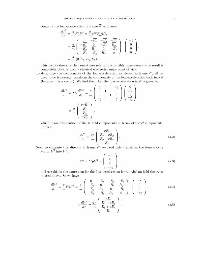
PHYSICS : GENERAL RELATIVITY HOMEWORK 7
compute the four-acceleration in frame O as follows:
dUa
dτ=
q
mF a
bUb =
q
mga℘F℘bU
b,
=q
m
0 −Ex −Ey −Ez
−Ex 0 −Bz By
−Ey Bz 0 −Bx
−Ez −By Bx 0
·
−1000
,
=q
m
(0, Ex, Ey, Ez
).
This results shows us that sometimes relativity is terribly unnecessary—the result iscompletely obvious from a classical electrodynamics point of view.
To determine the components of the four-acceleration as viewed in frame O, all weneed to do is Lorentz transform the components of the four-acceleration back into O
(because it is a vector). We find then that the four-acceleration in O is given by
dUa
dτ= Λa
a
dUa
dτ=
q
m
γ 0 0 vγ0 1 0 00 0 1 0vγ 0 0 γ
0Ex
Ey
Ez
,
=q
m
vγEz
Ez
Ey
γEz
,
which upon substitution of the O field components in terms of the O components,implies
dUa
dτ=
qγ
m
vEz
Ex − vBy
Ey + vBx
Ez
. (a.2)
Now, to compute this directly in frame O, we need only transform the four-velocityvector Ua into Ua,
Ua = ΛaaUa =
−γ00−vγ
, (a.3)
and use this in the expression for the four-acceleration for an Abelian field theory asquoted above. So we have
dUa
dτ=
q
mF a
bUb =
q
m
0 −Ex −Ey −Ez
−Ex 0 −Bz By
−Ey Bz 0 −Bx
−Ez −By Bx 0
·
−γ00−vγ
, (a.4)
∴
dUa
dτ=
qγ
m
vEz
Ex − vBy
Ey + vBx
Ez
. (a.5)

Physics , General RelativityHomework
Due Monday, th October
Jacob Lewis Bourjaily
Problem 1a) Let us consider the region of the t− x-plane which is bounded by the lines t = 0, t = 1, x = 0, and
x = 1; we are to find the unit outward normal one-forms and their associated vectors for each of theboundary lines.
It is not hard to see that the unit outward normal one-forms and their associated vectorsare given by
t = 0 : −dt 7→ ~et t = 1 : dt 7→ −~et; (1.a.1)
x = 0 : −dx 7→ −~ex x = 1 : dx 7→ ~ex. (1.a.2)
b) Let us now consider the triangular region bounded by events with coordinates (1, 0), (1, 1), and(2, 1); we are to find the outward normal for the null boundary and its associated vector.
The equation for the null boundary of the region is t = x + 1, which is specified by thevanishing of the function t − x − 1 = 0. The normal to the surface is simply thegradient of this zero-form, and so the normal is
dt− dx, (1.b.3)
and the associated vector is−~et − ~ex. (1.b.4)
Problem 2We are to describe the (proper orthochronous) Lorentz-invariant quantities that can be built out of the
electromagnetic field strength Fab and express these invariant in terms of the electric and magnetic fields.
Basically, any full contraction of indices will result in a Lorentz-invariant quantity. Fur-thermore, because we are considering things which are invariant under only properorthochronous transformation, we are free to consider CP -odd combinations, whichmix up components with their Hodge-duals. A list of such invariants are:
F aa = 0 F abFab = − (
?F ab)(?Fab) = 2
(~B2 − ~E2
) (?F ab
)Fab = −4 ~E · ~B. (2.a.1)
This does not exhaust the list of invariants, however: we are also free to take a numberof derivatives. These start getting rather horrendous, but we can start with an easyexample: (
∂aF ab)2
= 16π2JaJa = 16π2(
~J2 − ρ2)
. (2.a.2)
Along this vein, we find(∂aF ab
) (∂cF
cd)Fbd = 16π2 ~J ·
(~B × ~J
); (2.a.3)
[(∂aF ab
)F ab
]2= 16π2
ρ2 ~E2 −
(~E · ~J
)2
+(
~B × ~J)2
− 2ρ ~E ·(
~B × ~J)
; (2.a.4)
(∂aF ab
) (∂cF
cd)(?Fbd) = 16π2 ~J ·
(~E × ~J
). (2.a.5)
We could go higher in derivatives, but we know that ∂a ? F ab = 0 and we are free tomake the Lorentz gauge choice ¤F ab = 0. I suspect that further combinations willnot yield independent quantities.
1
2 JACOB LEWIS BOURJAILY
Problem 3Consider a pair of twins are born somewhere in spacetime. One of the twins decides to explore the
universe; she leaves her twin brother behind and begins to travel in the x-direction with constant ac-celeration a = 10 m/s2 as measured in her rocket frame. After ten years according to her watch, shereverses the thrusters and begins to accelerate with a constant −a for a while.
a) At what time on her watch should she again reverse her thrusters so she ends up home at rest?
There is an obvious symmetry in this problem: if it took her 10 years by her watch to gofrom rest to her present state, then 10 years of reverse acceleration will bring her torest, at her farthest point from home. Because of the constant negative acceleration,after reaching her destination at 20 years, she will begin to accelerate towards homeagain. In 10 more years, when her watch reads 30 years, she will be in the same stateas when her watch read 10 years, only going in the opposite direction.
Therefore, at 30 years, she should reverse her thrusters again so she arrives home in herhome’s rest frame.
b) According to her twin brother left behind, what was the most distant point on her trip?To do this, we need only to solve the equations for the travelling twin’s position and time
as seen in the stationary twin’s frame. This was largely done in class but, in brief,we know that her four-acceleration is normal to her velocity: aξuξ = 0 everywherealong her trip, and aξaξ = a2 is constant. This leads us to conclude that
at =dut
dτ= aux and ax =
dux
dτ= aut, (3.b.1)
where τ is the proper time as observed by the travelling twin. This system is quicklysolved for an appropriate choice of origin1:
t =1a
sinh (aτ) and x =1a
cosh (aτ) . (3.b.2)
This is valid for the first quarter of the twin’s trip—all four ‘legs’ can be givenexplicitly by gluing together segments built out of the above.
For the purposes of calculating, it is necessary to make aτ dimensionless. This is donesimply by
a =10 msec2
= 1.053 year−1. (3.b.3)
An approximate result2 could have been obtained by thinking of c = 3×10⁸ m/s and3× 107 sec = 1 year.
So the distance at 10 years is simply
x(10 yr) =1
1.053cosh (10.53) = 17710 light years.
The maximum distance travelled by the twin as observed by her (long-deceased) brotheris therefore twice this distance, or3
max(x) = 35, 420 light years. (3.b.4)
c) When the sister returns, who is older, and by how much?Well, in the brother’s rest frame, his sister’s trip took four legs, each requiring
t(10 yr) =1
1.053sinh (10.53) = 17710 years,
which means thatttotal = 70, 838 years. (3.c.5)
In contrast, his sister’s time was simply her proper time, or 40 years. Therefore thebrother who stayed behind is now 70, 798 years older than his twin sister.
1We consider the twin to begin at (t = 0, x = 1).2Because cosh goes like an exponential for large argument, our result is exponentially sensitive to the figures; because
we know c and the number of seconds per year to rather high-precision, there is no reason not to use the correct value ofa—indeed, the approximate value of a ∼ 1 year−1 gives an answer almost 40% below our answer.
3If we had used instead a = 1/year as encouraged by the problem set, our answer would have been 22, 027 light years.
PHYSICS : GENERAL RELATIVITY HOMEWORK 3
Problem 44
Consider a star located at the origin in its rest frame O emitting a continuous flux of radiation,specified by luminosity L.
a) We are to determine the non-vanishing components of the stress-energy tensor as seen by an ob-server located a distance x from the star along the x-axis of the star’s frame.
There are many ways to go about determining the components of the stress-energytensor. We will be un-inspired and compute it directly from the equation for theMaxwell stress-energy tensor (found by looking at metric variations of the Maxwellaction):
T ab = F acF
bc − 14ηabFabF
ab. (4.a.1)
We have in previous exercises computed all of the necessary terms, so we may simplyquote that
T 00 = ~E2 +12
(~B2 − ~E2
)=
12
(~B2 + ~E2
)= |~S|, (4.a.2)
T 0i =(
~E × ~B)i
= |~S|, (4.a.3)
where ~S is the Poynting vector, whose magnitude is just the energy density flux.Now, when we expand T xx, we find a bit more work in for us, at first glance, we see
T xx =32E2
x −12B2
x +12
(E2
y + E2z + B2
y + B2z
);
but we should note that because the radiation is only reaching the observer alongthe x-direction, ~S lies along the x-direction and so Bx = Ex = 0; therefore, we doindeed see that
T xx =12
(~B2 + ~E2
)= |~S|. (4.a.4)
And making use of the fact that ~S only has components in the x-direction, we seethat T 0y = T 0z = 0—with symmetrization implied.
Now, the energy density flux over a sphere centred about the origin of radius x naturallyis L
4πx2 . Therefore, we see that
∴ T 00 = T x0 = T 0x = T xx =L
4πx2. (4.a.5)
b) Let ~X be the null vector connecting the origin in O to event at which the radiation is measured.Let ~U be the velocity four-vector of the sun. We are to show that ~X → (x, x, 0, 0) and that T ab has theform
T =L
4π
~X ⊗ ~X(~U · ~X
)4 .
Well, it is intuitively obvious that if an observer sees radiation at (x, x, 0, 0), that, becauseit is null and forward-propagating, it must have been emitted from a source alongthe line τ(1, 1, 0, 0) where τ is an affine parameter for the world line of the photon.If it is the case that the photon was emitted by the sun that is sitting at x = 0, thenit must have been emitted at (0, 0, 0, 0), which means that ~X → (x, x, 0, 0).
Now, using the fact that ~U = (1, 0, 0, 0) for the star, we have that ~U · ~X = x, and this isframe-independent. Now, we see that ~X⊗ ~X only has components in (t, x)-directions
4This is the most poorly worded problem I have encountered thus far in this course. If there is any misunderstanding,I am strongly inclined to blame Schutz.
4 JACOB LEWIS BOURJAILY
and furthermore all the coefficients are the same, namely x2. Therefore
L
4π
~X ⊗ ~X(~U · ~X
)4 =L
4πx2(~et ⊗ ~et + ~et ⊗ ~et + ~ex ⊗ ~et + ~ex ⊗ ~ex) . (4.b.6)
Because this matches our explicit calculation in a certain frame and the expressionis manifestly frame-independent we see that this is a valid expression for T in anyreference frame5.
c) Consider an observer O travelling with speed v away from the star’s frame O in the x-direction.In that frame, the observation of radiation is at ~X → (R, R, 0, 0). We are to find R as a function of x
and express T 0x in terms of R.
There is no need to convert ~U of the sun into O’s coordinates because it only appears inT as a complete contraction—which is to say that ~U · ~X is frame independent. Now,all we need to do then is compute the coordinates of ~X in O’s coordinate system.This is done by a simple Lorentz transformation:
~X → O (xγ(1− v), xγ(1− v), 0, 0) ≡ (R, R, 0, 0), (4.c.7)
which is to say, R = xγ(1− v).Bearing in mind that the numerator in the expression of T was invariant, we see that
T 0x =L
4π
R2
x4. (4.c.8)
Now, inverting our expression for R, we see that
x2 =R2
γ2(1− v)2= R2
(1 + v
1− v
),
and so
∴ T 0x =L
4πR2
(1− v
1 + v
)2
. (4.c.9)
5Well, specifically, the difference between the T ab calculated above and the coordinate-free tensor vanishes identicallyat x; this tensor identity is obviously frame independent and so the tensors are identical.
Physics , General RelativityHomework
Due Wednesday, th October
Jacob Lewis Bourjaily
Problem 1Recall that the worldline of a continuously accelerated observer in flat space relative to some inertial
frame can be described by
t(λ, α) = α sinh(λ) and x(λ, α) = α cosh(λ), (1.a.1)
where λ is an affine parameter of the curve with αλ its proper length—i.e. the ‘time’ as measured byan observer in the accelerated frame. Before, we considered α to be constant and only varied λ. Weare now going to consider the entire (non-surjective) curvilinear map from two-dimensional Minkowskito-space to itself defined by equation (1.a.1).
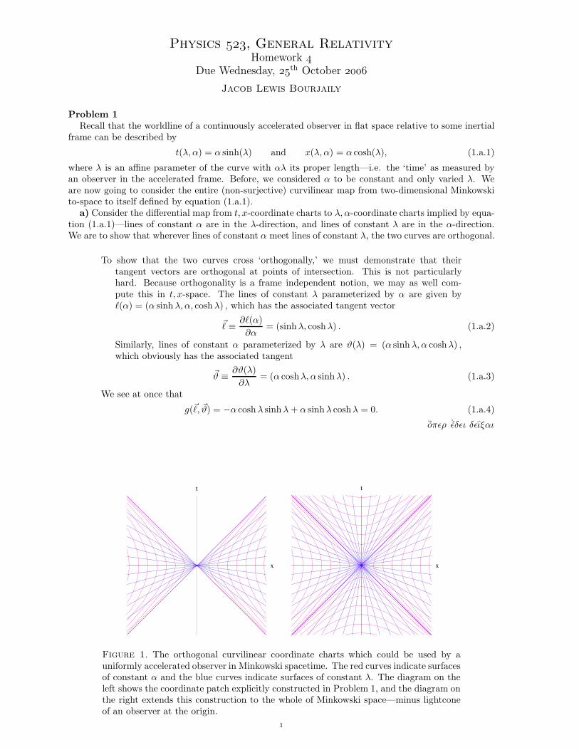
a) Consider the differential map from t, x-coordinate charts to λ, α-coordinate charts implied by equa-tion (1.a.1)—lines of constant α are in the λ-direction, and lines of constant λ are in the α-direction.We are to show that wherever lines of constant α meet lines of constant λ, the two curves are orthogonal.
To show that the two curves cross ‘orthogonally,’ we must demonstrate that theirtangent vectors are orthogonal at points of intersection. This is not particularlyhard. Because orthogonality is a frame independent notion, we may as well com-pute this in t, x-space. The lines of constant λ parameterized by α are given byℓ(α) = (α sinh λ, α, cosh λ) , which has the associated tangent vector
~ℓ ≡ ∂ℓ(α)
∂α= (sinhλ, coshλ) . (1.a.2)
Similarly, lines of constant α parameterized by λ are ϑ(λ) = (α sinh λ, α coshλ) ,which obviously has the associated tangent
~ϑ ≡ ∂ϑ(λ)
∂λ= (α coshλ, α sinh λ) . (1.a.3)
We see at once that
g(~ℓ, ~ϑ) = −α cosh λ sinh λ + α sinh λ coshλ = 0. (1.a.4)
‘oπǫρ ’ǫδǫι δǫιξαι
x
t
x
t
Figure 1. The orthogonal curvilinear coordinate charts which could be used by auniformly accelerated observer in Minkowski spacetime. The red curves indicate surfacesof constant α and the blue curves indicate surfaces of constant λ. The diagram on theleft shows the coordinate patch explicitly constructed in Problem 1, and the diagram onthe right extends this construction to the whole of Minkowski space—minus lightconeof an observer at the origin.
1
2 JACOB LEWIS BOURJAILY
b) We are to show that the map specified by equation (1.a.1) gives rise to an orthogonal coordi-nate system that covers half of Minkowski space in two disjoint patches. We should also represent thiscoordinate system diagrammatically.
From our work in part (a) above, we know that the tangent vectors to the lines ofconstant λ and α are given by
~eλ = α coshλ ~et + α sinh λ ~ex and ~eα = sinh λ ~et + coshλ ~ex. (1.b.1)
Therefore, the differential map (where greek letters are used to indicate λ, α-coordinates)is given by
Λµn =
(α cosh λ α sinh λsinh λ coshλ
). (1.b.2)
We see immediately that the Jacobian, det (Λ) = α 6= 0 which implies that the λ, αcoordinate system is good generically (where it is defined). That it is ‘orthogonal’ ismanifest because ~eλ · ~eα = 0 by part (a) above.
Note that the charts of (1.a.1) are not well-defined on or within the past or futurelightcones of an observer at the origin: the curves of α = constant, the hyperbolas,are all time-like and outside the past and future lightcones of an observer at theorigin; and the lines of λ = constant are all spacelike and coincident at the origin.It does not take much to see that these coordinates have no overlap within the pastand future lightcones of the Minkowski origin.
The coordinate system spanned by λ, α is shown in Figure 1.
c) We are to find the metric tensor and its associated Christoffel symbols of the coordinate chartsdescribed above.
Using equation (1.b.1), we can directly compute the components of the metric tensor inλ, α coordinates—gµν = g(~eµ, ~eν) where λ is in the ‘0’-position—
gµν =
(−α2 0
0 1
). (1.c.1)
The Christoffel symbols can be computed by hand rather quickly in this case; butwe will still show some rough steps. Recall that the components of the Christoffelsymbol Γµ
νρ are given by
Γµνρ~eµ =
(∂~eν
∂xρ
)µ
~eµ.
Again making use of equation (1.b.1), we see that
∂~eα
∂α= 0 =⇒ Γα
αα = Γλαα = 0. (1.c.2)
Slightly less trivial, we see
∂~eα
∂λ= coshλ ~et = sinh λ ~ex =
1
a~eλ =⇒ Γλ
αλ = Γλλα =
1
α; (1.c.3)
and,
∂~eλ
∂λ= α sinh λ ~et + α cosh λ~ex = α~eα =⇒ Γα
λλ = α, and Γλλλ = 0. (1.c.4)
‘oπǫρ ’ǫδǫι πoιησαι
PHYSICS : GENERAL RELATIVITY HOMEWORK 3
Problem 2We are to find the Lie derivative of a tensor whose components are T ab
c.
Although we are tempted to simply state the result derived in class and found in nu-merous textbooks, we will at least feign a derivation. Let us begin by recalling thatthe components of the tensor T are given by T ab
c = T(Ea,Eb,Ec) where the E’s arebasis vector- and one-form fields. Now, by the Leibniz rule for the Lie derivative weknow that
£X
(T(Ea,Eb,Ec)
)= £X(T)
(Ea,Eb,Ec
)+T
(£X(Ea) ,Eb,Ec
)+T
(Ea,£X
(Eb
),Ec
)+T
(Ea,Eb,£X(Ec)
).
(2.a.1)Now, the first term on the right hand side of equation (2.a.1) gives the componentsof £X(T), which is exactly what we are looking for. Rearranging equation (2.a.1) andconverting our notation to components, we see
(£X(T))ab
c = £X
(T ab
c
)− T αb
c (£X(Ea))α − T aβc
(£X
(Eb
))β− T ab
γ (£X(Ec))γ
. (2.a.2)
Now, we can either use some identities or just simply recall that
(£X(Ea))α =∂Xa
∂xαand (£X(Ec))
γ=
∂Xγ
∂xc. (2.a.3)
We now have all the ingredients; putting everything together, we have
(£X(T))ab
c = Xδ ∂
∂xδ
(T ab
c
)− T αb
c
∂Xa
∂xα− T aβ
c
∂Xb
∂xβ+ T ab
γ
∂Xγ
∂xc. (2.a.4)
‘oπǫρ ’ǫδǫι πoιησαι
Problem 3
Theorem: Acting on any tensor T, the Lie derivative operator obeys
£U£V(T) − £V£U(T) = £[U,V ](T). (3.a.1)
proof: We will proceed by induction. Let us suppose that the theorem holds for all tensorsof rank less than or equal to ( r
s) for some r, s ≥ 1. We claim that this is sufficientto prove the hypothesis for any tensor of rank
(r
s+1
)or
(r+1s
). (The induction
argument is identical for the two cases—our argument will depend on which index isadvancing—so it is not necessary to expound both cases.)
Now, all rank(
r+1s
)tensors can be written as a sum of tensor products between ( r
s)
rank tensors T indexed by i and rank(
10
)tensors E, again indexed by i1. That is,
we can express an arbitrary(
r+1s
)tensor as a sum of
∑i Ti ⊗Ei—where i is just an
index label! But this complication is entirely unnecessary: by the linearity of the Liederivative, it suffices to show the identity for any one tensor product in the sum.
Making repeated use of the linearity of the Lie derivative and the Leibniz rule, we see
(£U£V − £V£U) (T ⊗ E) =£U
((£VT) ⊗ E + T⊗ £VE
)− £V
((£UT) ⊗ E + T ⊗ £UE
),
=(£U£VT
)⊗ E + £VT ⊗ £UE + £UT ⊗ £VE + T ⊗
(£U£VE
)
−(£V£UT
)⊗ E− £UT ⊗ £VE− £VT ⊗ £UE − T⊗
(£V£UE
),
=(£[U,V ]T
)⊗ E + T ⊗
(£[U,V ]E
),
=£[U,V ]
(T ⊗ E
);
where in the second to last line we used the induction hypothesis—applicable becauseboth T and E are of rank ( r
s) or less.‘oπǫρ ’ǫδǫι δǫιξαι
1The savvy reader knows that an arbitrary ( rs) tensor can not be written as a tensor product of r contravariant and s
covariant pieces; however every ( rs) tensor can be written as a sum of such tensor products: indeed, this is exactly what
is done when writing ‘components’ of the tensor.
4 JACOB LEWIS BOURJAILY
It now suffices to show that the identity holds for all(
01
)forms and all
(10
)tensors2.
We will actually begin one-step lower and note that equation (3.a.1) follows triviallyfrom the Leibniz rule for 0-forms. Indeed, we see that for any 0-form f ,
£U(£Vf) =(£UV
)f + V
(£Uf
),
= £[U,V ]f + £V(£Uf) ,
∴
(£U£V − £V£U
)f = £[U,V ]f. (3.a.2)
Now, to finish our proof, we claim that the identity holds for any(
10
)and
(01
)tensors,
say X and Y, respectively. Recall that a one form Y is a function mapping vectorfields into scalars—i.e. Y(X) is a 0-form. For our own convenience, we will writeY(X) ≡ 〈X,Y〉. From our work immediately above, we know the identity holds for〈X,Y〉: (
£U£V − £V£U
)〈X,Y〉 = £[U,V ]
(〈X,Y〉
). (3.a.3)
Because the Leibniz rule obeys contraction, we can expand out the equation above similarto as before. Indeed, almost copying the equations above verbatim we find
(£U£V − £V£U) (〈X,Y〉) =£U
(〈(£VX) ,Y〉 + 〈X,£VY〉
)− £V
(〈(£UX) ,Y〉 + 〈X,£UY〉
),
= 〈£U£VX,Y〉 + 〈£VX,£UY〉 + 〈£UX,£VY〉 + 〈X,£U£VY〉− 〈£V£UX,Y〉 − 〈£UX,£VY〉 − 〈£VX,£UY〉 − 〈X,£V£UY〉 ,
=⟨(
£U£V − £V£U
)X,Y
⟩+
⟨X,
(£U£V − £V£U
)Y
⟩,
=⟨£[U,V ]X,Y
⟩+
⟨X,£[U,V ]Y
⟩.
In the last line, we referred to equation (3.a.3) and expanded it using the Leibniz rule.Almost a footnote-comment: the last two lines do not precisely prove our requiredtheorem as they stand: to identify the two pieces of each sum we need one smalltrick—replace one of X or Y with the basis one-forms or vector fields, and the resultfor the other becomes manifest.
Therefore, because equation (3.a.1) holds for all one-forms and vector fields, our induc-tion work proves that it must be true for all tensor fields of arbitrary rank. ‘oπǫρ ’ǫδǫι δǫιξαι
2You should probably suspect this is overkill: the induction step seemed to make no obvious use of the fact that r, s ≥ 1.And, as shown below, the identity is almost trivially true for the case of scalars. Nevertheless, it is better to be over-precisethan incorrect. (In the famous words of Blaise Pascal to a mathematician friend: “I have made this letter longer becauseI have not had the time to make it shorter.”)
PHYSICS : GENERAL RELATIVITY HOMEWORK 5
Problem 4The torsion and curvature tensors are defined respectively,
T (X, Y ) = ∇XY −∇Y X − £XY and R(X, Y ) = ∇X∇Y −∇Y ∇X −∇[X,Y ]. (4.a.1)
We are to prove
a) T (fX, gY ) = fgT (X, Y ),
b) R(fX, gY )hZ = fghR(X, Y )Z,
for arbitrary functions f, g and h, and vector fields X, Y and Z.
Theorem a: T (fX, gY ) = fgT (X, Y ).
proof: In both of the required proofs, we will make repeated uses of the ‘defining’ propertiesof the covariant derivative ∇ and of the Lie derivative. In particular, we will needthe following properties of the connection:(1) ∇XY is a tensor in the argument X . This means that as an operator, ∇fX+gY =
f∇X + g∇Y .(2) ∇XY obeys the Leibniz rule in Y . Specifically, this means ∇X(fY ) = X(f)Y +
f∇XY . This implies that ∇XY is linear in Y —which follows when f is a con-stant.
We are almost ready to ‘prove the identity by brute force in a couple of lines.’ Let’s justprepare one more trick up our sleeve: we will need
[fX, gY ] = £fX(gY ) = g£fXY +(£fXg
)Y,
= −g£Y(fX) + fX(g)Y,
= −gfY (X) − gXY (f) + fX(g)Y.
Let us begin:
T (fX, gY ) = ∇fX(gY ) −∇gY (fX) − £fX(gY ) ,
= f∇X(gY ) − g∇Y (fX) − £fX(gY ) ,
= fX(g)Y + fg∇XY − g(Y (f))X − fg∇Y X + gfY (X) + gXY (f) − fX(g)Y,
= fg∇XY − fg∇Y X − gf£XY,
∴ T (fX, gY ) = fgT (X, Y ). (4.a.2)
‘oπǫρ ’ǫδǫι δǫιξαι
Theorem b: R(fX, gY )hZ = fghR(X, Y )Z.
proof: We have already collected all of the properties and identities necessary to straight-forwardly prove the theorem. Therefore, we may proceed directly.
R(fX, gY )hZ =∇fX∇gY −∇gY ∇fX −∇[fX,gY ]
hZ,
=f∇X (g∇Y ) − g∇Y (f∇X) − fg∇[X,Y ] − f∇Y X(g) + g∇XY (f)
hZ,
=fX(g)∇Y + fg∇X∇Y − gY (f)∇X − fg∇Y ∇X − fg∇[X,Y ] − fX(g)∇Y + gY (f)∇X
hZ,
=fg∇X∇Y − fg∇Y ∇X − fg∇[X,Y ]
hZ,
=fgR(X, Y )hZ,
=fg∇X
(Y (h)Z + h∇Y Z
)−∇Y
(X(h)Z + h∇XZ
)− [X, Y ] (h)Z − h∇[X,Y ]Z
,
=fg∇X
(Y (h)Z
)+ X(h)∇Y Z + h∇X∇Y Z −∇Y
(X(h)Z
)− Y (h)∇XZ − h∇Y ∇XZ
− X (∇Y h)Z + Y (∇Xh)Z − h∇[X,Y ]Z,
=fghR(X, Y )Z + (∇X (Y (h)))Z −∇Y (X(h))Z − X (Y (h)) Z + Y (X(h))Z
,
∴ R(fX, gY )hZ = fghR(X, Y )Z. (4.b.1)
‘oπǫρ ’ǫδǫι δǫιξαι

Physics , General RelativityHomework
Due Friday, th November
Jacob Lewis Bourjaily
Problem 1Let us consider a manifold with a torsion free connection R(X, Y ) which is not necessarily metric
compatible. We are to prove that
R(X, Y )Z + R(Y, Z)X + R(Z, X)Y = 0, (1.1)
and the Bianchi identity
∇X
(R(X,Y )
)V +∇Y
(R(Z,X)
)V +∇Z
(R(X,Y )
)V = 0. (1.2)
The first identity is relatively simple to prove—it follows naturally from the Jacobiidentity for the Lie derivative. Let us first prove the Jacobi identity:
[X, [Y, Z]] + [Y, [Z,X]] + [Z, [X, Y ]] = 0. (1.3)
Using the antisymmetry of the Lie bracket and our result from last homework problem3, we have
[X, [Y,Z]] = £X[Y, Z] = −£[Y,Z]X = £Z£YX −£Y£ZX = −[Z, [X, Y ]]− [Y, [Z,X]].‘oπερ ’εδει δειξαι
The condition of a connection being torsion free is that
£XY = ∇XY −∇Y X. (1.4)
Expanding the Lie brackets encountered in the statement of the Jacobi identity,
0 =£X£YZ + £Y£ZX + £Z£XY,
=£X(∇Y Z −∇ZY ) + £Y (∇Y X −∇XY ) + £Z(∇XY −∇Y X) ,
=∇X∇Y Z −∇X∇ZY −∇[Y,Z]X +∇Y∇ZX −∇Y∇XZ −∇[Z,X]Y +∇Z∇XY −∇Z∇Y X −∇[X,Y ]Z,
=(∇X∇Y −∇Y∇X −∇[X,Y ]
)Z +
(∇Y∇Z −∇Z∇Y −∇[Y,Z]
)X +
(∇Z∇X −∇X∇Z −∇[Z,X]
)Y ;
∴ R(X,Y )Z + R(Y, Z)X + R(Z, X)Y = 0. (1.5)‘oπερ ’εδει δειξαι
To prove the Bianchi identity, we will ‘dirty’ our expressions with explicit indices inhope of a quick solution. It is rather obvious to see that (1.2) is equivalent to thecomponent expression
Rabcd;e + Ra
bde;c + Rabec;d = 0. (1.6)
Worse than introducing components, let us use our (gauge) freedom to consider theBianchi identity evaluated at a point p in spacetime in Riemann normal coordinates1.If we show that the Bianchi identity (1.6) holds in any particular coordinates at apoint p, it necessarily must hold in any other coordinate system—and if p is arbitrary,then it follows that the Bianchi identity holds throughout spacetime.
Recall from lecture or elsewhere that Riemann normal coordinates at p are such thatΓa
bc(p) = 0. This implies that the covariant derivative of the Riemann tensor is simplya normal derivative at p. Using the definition of Ra
bcd in terms of the Christoffelsymbols, we see at once that
Rabcd;e(p) + Ra
bde;c(p) + Rabec;d(p) = Γa
bd,ce(p)− Γabc,de(p) + Γa
be,dc(p)− Γabd,ec(p) + Γa
bc,ed(p)− Γabe,cd(p);
∴ Rabcd;e(p) + Ra
bde;c(p) + Rabec;d(p) = 0. (1.7)
‘oπερ ’εδει δειξαι
1Riemann normal coordinates are constructed geometrically as follows: in a sufficiently small neighbourhood about p,every point can be reached by traversing a certain geodesic through p a certain distance. If we choose to define all familiesof geodesics through p using the same affine parameter λ then if we fix λ, there is a (smooth) bijection between tangentvectors in TpM to points in the neighbourhood about p: the direction of v ∈ TpM tells the direction to the nearby pointsand its magnitude (for fixed λ) tells the distance to travel along the geodesic. Needless to say this construction does notrequire a metric.
1
2 JACOB LEWIS BOURJAILY
Problem 2We are to compute the Riemann tensor, the Ricci tensor, the Weyl tensor and the scalar curvature
of a conformally-flat metric,gab(x) = e2Ω(x)ηab. (2.1)
Using the definition of the Christoffel symbol with our metric above, we find
Γabc =
12gam gam,b + gbm,a − gab,m ,
=12e−2Ωηam
ηbme2Ω∂cΩ + ηcme2Ω∂bΩ− e2Ωηbc∂mΩ
,
∴ Γabc = δa
b ∂cΩ + δac ∂bΩ− ηbcη
am∂mΩ. (2.2)Using this together with the (definition of the) Riemann tensor’s components
Rabcd = Γa
bd,c − Γabc,d + Γm
bdΓacm − Γm
bcΓadm, (2.3)
we may compute directly2,
Rabcd = δa
d∂c∂bΩ− ηbdηam∂c∂mΩ− δa
c ∂b∂dΩ + ηbcηam∂d∂mΩ− δa
d (∂bΩ) (∂cΩ) + ηbdηam(∂cΩ)(∂mΩ)
− δad(∂cΩ)(∂bΩ)− δa
c (∂bΩ)(∂bΩ) + ηbcδadηmn(∂mΩ)(∂nΩ) + δa
c (∂bΩ)(∂dΩ)− ηbcηam(∂dΩ)(∂mΩ)
+ δac (∂dΩ)(∂bΩ) + δa
d(∂bΩ)(∂cΩ)− ηbddacηmn(∂mΩ)(∂nΩ)− ηbdη
am(∂cΩ)(∂mΩ) + ηbdηam(∂cΩ)(∂mΩ)
=
δmb (δa
c δnd − δa
dδnc ) + ηbd (ηanδm
c − ηmnδac ) + ηbc (ηmnδa
d − ηanδmd )
(∂mΩ) (∂nΩ)
+ (δad∂c − δa
c ∂d) ∂bΩ + ηam (ηbc∂d∂mΩ− ηbd∂c∂mΩ) .
‘oπερ ’εδει πoιησαι
It will be helpful to recast this into the form where all the indices are lowered. We cando this by acting with the metric tensor. Doing so we find,
e−2ΩRabcd =
δmb (ηacδ
nd − ηadδ
nc ) + ηbd (δn
a δmc − ηacη
mn) + ηbc (ηadηmn − δm
a δnd )
(δmΩ)(δnΩ)
+ ηad∂c∂bΩ− ηac∂d∂bΩ + ηbc∂d∂aΩ− ηbd∂c∂aΩ,
=
ηadδmb δn
c − ηacδmb δn
d + ηbcδma δn
d − ηbdδma δn
c
(∂m∂nΩ− (∂mΩ)(∂nΩ)
)+
(ηadηbc − ηacηbd
)ηmn(∂mΩ)(∂nΩ).
(2.4)
Although we will not have any use for such frivolities, we can further compress thisexpression to
e−2ΩRabcd = 4δr[a δn
b]δs[d δm
c]ηrs
(∂m∂nΩ− (∂mΩ)(∂nΩ)
)+
(ηadηbc − ηacηbd
)ηmn(∂mΩ)(∂nΩ). (2.5)
Now, we can then find the Ricci tensor by acting on equation (2.4) with gac. Letting Dbe the dimensionality of our manifold, we find
Rbd =
δmd δn
b −Dδmd δn
b + δmd δn
b − ηbdηmn
(∂m∂nΩ− (∂mΩ)(∂nΩ)
)+ ηmn
(ηbd −Dηbd
)(∂mΩ)(∂nΩ),
=(2−D)(∂b∂dΩ− (∂bΩ)(∂dΩ)
)+ (2−D)ηbdη
mn(∂mΩ)(∂nΩ)− ηbdηmn∂m∂nΩ. (2.6)
‘oπερ ’εδει πoιησαι
Lastly, contracting this, we find the scalar curvature,
e2ΩR =(2−D)ηmn(∂m∂nΩ− (∂mΩ)(∂nΩ)
)+ D(2−D)ηmn(∂mΩ)(∂nΩ)−Dηmn∂m∂nΩ,
=2(1−D)ηmn∂m∂nΩ− (2−D)(1−D)ηmn(∂mΩ)(∂nΩ). (2.7)‘oπερ ’εδει πoιησαι
2To be absolutely precise, there are two terms which manifestly cancel that appear when expanding this expression,which we have left out for typographical and aesthetic considerations.
PHYSICS : GENERAL RELATIVITY HOMEWORK 3
All that remains for us to compute is the Weyl tensor. Any exposure to conformalgeometry immediately tells us that the Weyl tensor vanishes. That is, that
Rabcd =1
(D − 2)
(gacRdb + gdbRac − gadRbc − gbcRad
)− 1
(D − 1)(D − 2)R
(gacgdb − gadgbc
). (2.8)
We will try as hard as possible to avoid actually computing the right hand side byexpanding our expressions above. To show that the Weyl tensor vanishes, we mustbuild Rabcd out of Rbc, R and the metric gab. This statement alone essentially givesus the expression at first glance.
The first important thing to notice is that Rabcd has no term proportional to ηmn∂m∂nΩwhile both Rab and R do. This means that if Rabcd can only be composed of linearcombinations of Rab and R which do not contain ηmn∂m∂nΩ. Looking at expressions(2.4) and (2.6), we see that they can only appear in the combination
Rbd +e2Ωηbd
2(1−D)R = Rbd +
gbd
2(1−D)R. (2.9)
Any multiple of this combination will automatically have no ηmn∂m∂nΩ contribution.Staring a bit more at equations (2.4) and (2.6), we notice that the first set of terms in
(2.4) are all of the form gacRbd. Indeed, we see that1
2−D
ηadRbc−ηacRbd+ηbcRad−ηbdRac
=
ηadδ
mb δn
c−ηacδmb δn
d +ηbcδma δn
d−ηbdδma δn
c
(∂m∂nΩ−(∂mΩ)(∂nΩ)
)+. . . .
(2.10)Notice that multiplying both sides of the above equation by e2Ω will convert all ofthe ηab’s into gab’s3 . This is all we need to construct the Riemann tensor from theRicci tensor and scalar curvature: knowing the combination of Ricci tensors whichgives part of the Riemann tensor, we can use (2.9) to determine the rest. Indeed, wesee that
Cabcd + Rabcd =1
2−D
gabRbc − gadRbd + gbcRad − gbdRac
+
R
2(1−D)(2−D)
(gadgbc − gacgbd + gbcgad − gbdgac
),
=1
D − 2
gacRbd − gadRbc − gbcRad + gbdRac
− R
(D − 1)(D − 2)
(gacgbd − gadgbc
),
=
gadδmb δn
c − gacδmb δn
d + gbcδma δn
d − gbdδma δn
c
(∂m∂nΩ− (∂mΩ)(∂nΩ)
)+
(gadgbc − gacgbd
)gmn(∂mΩ)(∂nΩ),
=Rabcd;
∴ Cabcd = 0. (2.11)‘oπερ ’εδει πoιησαι
3The conversion from ηab → gab is completely natural. The only possibly non-trivial step comes from the last termin the expression (2.4) for the Riemann tensor: bringing e2Ω to the right hand side of (2.4), we have a term which hastwo lowered ηab’s and one upper ηab; now, e2Ωηmn = e4Ωgmn and how these two factors of e2Ω can be absorbed into thelowered η’s as desired.
4 JACOB LEWIS BOURJAILY
Problem 3We are to show that if ϕ(x) satisfies the flat-space, massless Klein-Gordon equation, then if gab =
e2Ω(x)ηab, the transformed field eβΩ(x)ϕ(x) ≡ ϕ′(x) satisfies the equation
gabϕ′;ab − αRϕ′ = 0, (3.1)
for appropriate values of α and β—dependant on the spacetime dimension but independent of Ω(x).
Let us agree to call ¤ ≡ ηab∂a∂b. Then the flat-space Klein-Gordon equation is sim-ply ¤ϕ(x) = 0. Recall the expression for the scalar curvature R in D spacetimedimensions for a metric which is conformally-related to the Minkowski metric (2.7):
R = 2(1−D)e−2Ω¤Ω− (2−D)(1−D)e−2Ωηmn(∂mΩ)(∂nΩ). (3.2)
We would like to explicitly state gab∇b∇a in terms of ¤ and Ω. This can be done quiteexplicitly, recalling the Christoffel symbols for a conformally-flat spacetime(2.2),
gab∇b∇a = gab∂a∂b − gabΓcab∂c,
= e−2Ω
¤− ηab(δca(∂bΩ)∂c + δc
b(∂aΩ)∂c − ηabηcm(∂mΩ)∂c
),
= e−2Ω
¤− ηcb(∂bnΩ)∂c − ηac(∂aΩ)∂c + Dηcm(∂mΩ)∂c
,
= e−2Ω
¤− (D − 2)ηab(∂aΩ)∂b
.
Acting with gab∇b∇a on ϕ′ we find,
gab∇b∇aϕ′ = e−2Ω
¤(eβΩϕ
)+ (D − 2)ηab(∂aΩ)
(∂b
(eβΩϕ
)) ,
= e−2Ω
βϕ′¤(Ω) + β(β + D − 2)ϕ′ηab(∂aΩ)(∂bΩ) + 2βeβΩηab(∂aϕ)(∂bΩ) + (D − 2)eβΩηab(∂aϕ)(∂bΩ)
.
Although only one equation, if (3.1) is to hold for arbitrary Ω(x), there are actuallythree constraints implied by (3.1)—one for each functionally distinct contribution.Actually, we’ll find that there are only two independent conditions—just enough touniquely determine α and β.
First, notice that R does not contain any derivatives of ϕ(x). Therefore equation (3.1)implies that
2βeβΩηab(∂aϕ)(∂bΩ) + (D − 2)eβΩηab(∂aϕ)(∂bΩ) = 0, (3.3)
arising from the gab∇b∇aϕ′ term in (3.1). This obviously implies that
∴ β = −D − 22
. (3.4)
The next condition(s) come form matching the remaining two functionally distinct termsin (3.1), namely4
gab∇b∇aϕ′−αRϕ′ ∝ β¤Ω+β(β+D−2)ηab(∂aΩ)(∂bΩ)−2α(1−D)¤Ω+α(D−2)(D−1)ηab(∂aΩ)(∂bΩ).(3.5)
Matching the corresponding terms, we see that
α =β
2(1−D)and α =
−β(β + D − 2)(D − 2)(D − 1)
. (3.6)
We see that β = 12 (D−2) is consistent with both of these—more concretely, any two
of these three constraints is sufficient to imply the third. Therefore, we have shownthat ϕ′ = eβΩϕ will satisfy the modified Klein-Gordon equation (3.1) for any Ω(x) if
∴ β =2−D
2and α =
14
D − 2D − 1
. (3.7)
‘oπερ ’εδει πoιησαι
4We are not including those pieces eliminated by the choice (3.4).
Physics , General RelativityHomework
Due Wednesday, th November
Jacob Lewis Bourjaily
Problem 11
We are asked to determine the ratio of frequencies observed at two fixed2 points in a spacetime witha static metric gab; we should use this to determine the redshift of light emitted from the surface of theSun which is observed on the surface of the Earth.
Imagine a clock at a fixed point x1 which ticks with a regular interval ∆s. Because thepoint is stationary, we may use the definition of the spacetime metric gab to see thatthis interval is related to the coordinate time interval ∆t by3
∆s2 = ∆t21g00(x1). (1.1)
We have included a subscript on the coordinate time interval to make its position-dependence manifest. The invariant interval ∆s, however, must certainly be position-independent for any reliable clock. Therefore, we naturally have that
∆s2 = ∆t21g00(x1) = ∆t22g00(x2), (1.2)
for any other point x2. This implies that
∴ ∆t21∆t22
=g00(x2)g00(x1)
. (1.3)
It is important to note that this discussion is not limited to clocks ticking regularly: anyprocess with a well-defined, constant time interval observed at two distinct pointswill obey equation (1.3). Indeed, consider an atomic transition which emits photonswith frequency ν1 ≡ 1
∆t1at point x1. Equation (1.3) implies that the frequency at
x1 will be related to the frequency ν2 at x2 by
∴ ν2
ν1=
√g00(x2)g00(x1)
. (1.4)
‘oπερ ’εδει πoιησαι
To determine the redshift of light emitted from the Sun and observed on the Earth werecall that in the Newtonian (weak-field) approximation,
g00(x) = −1− 2ϕN (x), (1.5)
where ϕN (x) is the Newtonian potential at x. The only subtlety is that we shouldmake sure to be careful about units when computing ϕN (x). Notice that becausethe ‘1’ in −1− 2ϕN (x) is dimensionless, so should ϕN (x) be. This will be the case ifwe judiciously set c = 1. In these units, we find
ϕN (R¯) = −2.12× 10⁻⁶ and ϕN (R⊕) = −1.06× 10⁻⁸, (1.6)
which gives a redshift of 2.11 parts per million.
1Note added in revision: this solution is bad. The argument presented for equation (1.4) is not valid (even though theright answer emerges). One should be very careful about the thought experiment under consideration (because the inverseresult is easy to obtain under a different situation).
2The equation which the problem set asks us to demonstrate is only valid for stationary sources and observers—otherwisethere would be a doppler-shift term obfuscating the equation.
3In his textbook, Weinberg has an interesting discussion on why it is fundamentally not possible to disentangle ∆s from∆t at a particular point. However, it is possible to compare the metric at two distinct points—by observing a gravitationalredshift—as described presently.
1
2 JACOB LEWIS BOURJAILY
Problem 2We are to find the ‘natural’ generally covariant generalization of the flat-space Klein-Gordon La-
grangian (which was shown to be Weyl invariant in the last problem set). We should use this todetermine the matter stress-energy tensor and show that it is traceless.
The striking similarity between
gab∇a∇bϕ− 16Rϕ = 0, (2.1)
and the massive Klein-Gordon equation makes us guess that the action from whichthis is derived is
S =12
∫d4x
√−ggab
(∇aϕ∇bϕ +
16Rabϕ
2
). (2.2)
Our intuition is confirmed by calculating the equation of motion:
0 = ∇a
(∂L
∂∇aϕ
)− ∂L
∂ϕ= ∇a
(gab∇bϕ
)− 16Rϕ,
= gab∇a∇bϕ− 16Rϕ. (2.3)
Therefore the action (2.2) does indeed give rise to the desired equation of motion forϕ as desired.
We now must compute the stress-energy tensor for this matter Lagrangian. Recall thatthe stress-energy tensor T ab of a system with action S is defined according to
δS =12
∫d4x
√−g T abδgab, (2.4)
from the variation gab 7→ gab + δgab. To compute the metric variation for the actiongiven in (2.2) we first recall some useful identities:
δgab = −gacgbdδgcd; δ(√−g) =
12√−ggabδgab; (2.5)
and gabδRab = ∇awa, where wa ≡ ∇b (δgab)− gcd∇a (δgcd) . (2.6)
This last identity, (2.6), follows from work done in lecture. Although brevity temptsus to simply quote Wald’s textbook, it is sufficiently important to warrant a fullderivation. Therefore, to please the reader, a proof of this identity has been includedas an Appendix to this problem set.
We are now prepared to compute the metric variation of the action (2.2). As we proceed,any total divergence will be assumed to integrate to zero.
δS =12
∫d4x
√−g
12gabδgabg
cd
(∇cϕ∇dϕ +
16Rcdϕ
2
)+ δgab
(∇aϕ∇bϕ +
16Rabϕ
2
)+
16gabδRabϕ
2
,
=12
∫d4x
√−g
[δgab
12gabgcd
(∇cϕ∇dϕ +
16Rcdϕ
2
)−
(∇aϕ∇bϕ +
16Rabϕ2
)+
16gcdδRcdϕ
2
],
=12
∫d4x
√−g
[δgab
12gabgcd
(∇cϕ∇dϕ +
16Rcdϕ
2
)−
(∇aϕ∇bϕ +
16Rabϕ2
)+
16
(∇cwc)ϕ2
],
=12
∫d4x
√−g
[δgab
12gabgcd
(∇cϕ∇dϕ +
16Rcdϕ
2
)−
(∇aϕ∇bϕ +
16Rabϕ2
)− 1
6(∇cϕ2
)wc
].
(2.7)
The last term in the expression above is qualitatively different from the first two. Letus try to recast it into a form which makes the δgab-dependence manifest. Using thedefinition of wc and making repeated use of integration by parts, we see∫
d4x√−g ∇a(ϕ2)wa =
∫d4x
√−g ∇a(ϕ2)(∇b (δgab)− gcd∇a (δgcd)
),
=∫
d4x√−g
(∇b
(δgab∇a(ϕ2)
)− δgab∇b
(∇a(ϕ2)
)− gcd∇a
(δgcd∇a(ϕ2)
)+ gabδgab∇c
(∇c(ϕ2)
)),
=∫
d4x√−g δgab
(gabgcd∇c∇dϕ
2 −∇a∇bϕ2). (2.8)
PHYSICS : GENERAL RELATIVITY HOMEWORK 3
We are now ready to put everything together and find T ab. To make our result a bitmore transparent, let us agree to call gcd∇c∇d ≡ 2. Also, the identity gcd∇cϕ∇dϕ =122ϕ2 − ϕ2ϕ will allow us to tidy up our expressions substantially. Combining allof this, we can continue our work on the total variation (2.7) using the result from(2.8) to find
δS =12
∫d4x
√−gδgab
12gabgcd
(∇cϕ∇dϕ +
16Rcdϕ
2
)−
(∇aϕ∇bϕ +
16Rabϕ2
)− 1
6
(gabgcd∇c∇dϕ
2 −∇a∇bϕ2)
,
=12
∫d4x
√−gδgab
12gabgcd
(∇cϕ∇dϕ− 1
3∇c∇dϕ
2 +16Rcdϕ
2
)−∇aϕ∇bϕ− 1
6Rabϕ2 +
16∇a∇bϕ2
,
=12
∫d4x
√−gδgab
12gab
(162ϕ2 +
16Rϕ2 − ϕ2ϕ
)− 1
3∇a∇bϕ2 + ϕ∇a∇bϕ− 1
6Rabϕ2
. (2.9)
This allows us to read-off
∴ T ab =12gab
(162ϕ2 +
16Rϕ2 − ϕ2ϕ
)− 1
3∇a∇bϕ2 + ϕ∇a∇bϕ− 1
6Rabϕ2. (2.10)
‘oπερ ’εδει πoιησαι
As anyone who’s seen conformal field theory knows, the trace of the stress-energy tensormust vanish. Let’s see how this ‘magically’ works out in the situation consideredpresently.
gabTab =
132ϕ2 +
13Rϕ2 − 2ϕ2ϕ− 1
32ϕ2 + ϕ2ϕ− 1
6Rϕ2,
=16Rϕ2 − ϕ2ϕ,
= −ϕ
(2ϕ− 1
6Rϕ
),
= 0.
Notice that the last line required using the equations of motion—which wasn’t entirelyanticipated—at least by us.
4 JACOB LEWIS BOURJAILY
Problem 3: Killing Vectors
a. If ζa(x) is a Killing field and pa(λ) is the tangent vector to a geodesic curve γ(λ), then paζa(x)is constant along γ.
proof: The derivative of paζa along γ is
pb∇b (paζa) = papb∇bζa + ζapb∇bpa. (3.1)
The first term vanishes because papb is symmetric while ∇bζa is antisymmetric (be-cause it is Killing). The second term vanishes because pa is the tangent of a ge-odesic, which practically by definition implies that it obeys the geodesic equation,pb∇bp
a = 0. ‘oπερ ’εδει δειξαι
b. We are to list the ten independent Killing fields of Minkowski spacetime.
The ten independent Killing fields correspond to the ten generators of the Poincarealgebra: four translations, three rotations, and three boosts. Given in terms of thebasis vectors ~ea, we the Killing vector fields are therefore
Translations : ~et, ~ex, ~ey, ~ez;
Rotations : y~ex − x~ey, z~ey − y~ez, x~ez − z~ex;
Boosts : x~et + t~ex, y~et + t~ey, z~et + t~ez;
Each of these ten vector fields manifestly satisfies Killing’s equation. That they arelinearly independent is also manifest4.
c. If ζa and ηa are Killing fields and α, β constants, then αζa + βηa is Killing.proof: As should be obvious to all but the most casual observer,
∇b (αζa + βηz) = α∇bζa + β∇bηa = −α∇aζb − β∇aηb = −∇a (αζb + βηb) , (3.2)
because, being constants, α, β commute with the gradient and ζa, ηa are Killing.Therefore equation (3.2) implies that (αζa + βηa) is Killing. ‘oπερ ’εδει δειξαι
d. We are to show that Lorentz transformations of the Killing vector fields listed in part (b) abovegive rise to linear recombinations of the same fields with constant coefficients.
Because every Lorentz transformation can be built from infinitesimal ones, it is sufficientto demonstrate the claim for infinitesimal Lorentz transformations. And this makesour work exceptionally easy. Infinitesimal Lorentz transformations are simply theidentity plus a constant multiple of the generators of the Lorentz algebra; but (the lastsix of) the Killing fields listed in part (b) are nothing but these Lorentz generators.
Therefore, any infinitesimal Lorentz transformation of the Killing fields listed in part (b)is a linear combination of those same Killing fields with constant coefficients. Andby extension, the same is true for any finite Lorentz transformation.
4Although we should add that we were not requested to demonstrate this—so our lack of exposition here should beforgiven.
PHYSICS : GENERAL RELATIVITY HOMEWORK 5
Appendix
In problem 2 we made use of an identity that didn’t obviously follow from the work in lecture. Weremedy that deficiency presently5.
Lemma: Under the variation gab 7→ gab + δgab,
gabδRab = ∇awa, where wa ≡ ∇b (δgab)− gcd∇a (δgcd) . (A.1)
proof: We may begin with the related expression derived in lecture,
gabδRab = ∇a
(gbcδΓa
bc − gacδΓbcb
). (A.2)
Rearranging this we find
gabδRab = ∇a
gbcgadδΓdbc − δΓd
ad
; (A.3)
therefore, it suffices to show that the term in brackets is equal to wa. Expanding thisexpression and using symmetry to collect and cancel terms, we find
gbcgadδΓdbc − δΓd
ad =12gbcgadδg
de(gbe,c + gce,b − gbc,e
)+
12gbcδe
a
(δgbe,c + δgce,b − δgbc,e
)
− 12δgbe
(gae,b + gbe,a − gab,e
)− 1
2gbe
(δgae,b + δgbe,a − δgab,e
),
=− 12gbcgefδd
aδgde
(gbf,c + gcf,b − gbc,f
)+
12gbc
(δgba,c + δgca,b − δgbc,a
)+
12δgdeg
dcgefgcf,a − 12gbeδgbe,a,
=− gbcgefδdaδgdegbf,c − 1
2gbcgefδd
aδgdegbc,f + gbcδgba,c − 12gbcδgbc,a +
12δgdeg
dcgefgcf,a − 12gbcδgbc,a,
=gbcδgba,c − gbcδgbc,a − gbcgefgbf,cδgae − 12gbcgefgbc,fδgae +
12gdcgefgcf,aδgde.
Expanding the first two terms in the expression above in terms of covariant derivativesand Christoffel symbols, we observe
gbcδgab,c = ∇b (δgab) + gbcδgebΓeac + gbcδgaeΓe
bc, (A.4)
andgbcδgbc,a = gbc∇a (δgbc) + gbcδgbeΓe
ac + gbcδgecΓeba. (A.5)
Noting that the terms with the covariant derivatives are what we are looking for—together, they give wa. Putting everything together,
gbcgadδΓdbc − δΓd
ad = wa +
gbcδgaeΓebc − gbcδgecΓe
ba + gbcgef
(12gfc,aδgbe +
12gbc,fδgae − gbf,cδgae
).
(A.6)All that remains is for us to show that the terms in curly brackets above vanish. To do
this, we will expand our expressions one last time—this time using the definition ofthe Christoffel symbols for a metric connection. Doing so, we find
gbcgadδΓdbc − δΓd
ad − wa = gbcgef
12gfc,aδgbe +
12gbc,fδgae − gbf,cδgae
− 12gbf,aδgec − 1
2gaf,bδgec +
12gba,fδgec
+12gbf,cδgae +
12gcf,bδgae − 1
2gbc,fδgae
,
= 0.
Here we have indicated the terms that cancel together in matching colours. Withthis, we have shown that
∴ gabδRab = ∇a
gbcgadδΓdbc − δΓd
ad
= ∇a
∇b (δgab)− gcd∇a (δgcd)
= ∇awa. (A.7)
‘oπερ ’εδει δειξαι
5We hope that there is an easier way to prove the following Lemma. But alas! too little time to be brief. Breviloquenceis a time-consuming luxury.

Physics , General RelativityHomework
Due Wednesday, th December
Jacob Lewis Bourjaily
Problem 1Consider a gyroscope moving in circular orbit of radius R about a static, spherically-symmetric planet
of mass m.a. We are to derive the equations of motion for the gyroscopic spin vector as a function of azimuthal
angle and show that the spin precesses about the direction normal to the orbital plane.
This calculation will be far from elegant, and will probably not give rise to much insight.Nevertheless, we start by recalling the Lagrangian describing a particle’s worldline(inthe θ = π
2 plane) in a static, isotropic spacetime,
L = −gabuaub = f(r)(ut)2 − 1
f(r)(ur)2 − r2(uϕ)2, (1.1)
where ua ≡ dxa
dτ for some affine parameter τ . Because our analysis will be limitedto circular geodesics, we will not have much use for the ur coordinate; however,its equation of motion will be necessary to relate the various integrals of motion.First observe that uϕ is non-dynamical in the Lagrangian and so it gives us our firstintegral of motion,
J ≡ r2uϕ. (1.2)
For circular geodesics, ua will of course only have 0 and ϕ components; ut is also non-dynamical, and so we are free to set ut by the normalization of the affine parameterτ :
u2 = −gabuaub = f(R)(ut)2 − J2
R2≡ 1, =⇒ ut =
√1
f(R)
(1 +
J2
R2
). (1.3)
Now, it is easy to see that the equation of motion for the r-component is
−2r
f(r)+ 2
r2
f2(r)f ′(r) = − r2
f2(r)− 2
J2
r3+ f ′(r)(ut)2. (1.4)
Because we are looking for solutions where both r and r vanish—and r = R—we seeat once that this implies the relation
J2 =12f ′(R)(ut)2R3 =
m
R2
R4
(R− 2m)
(1 +
J2
R2
),
=mR2
R− 2m
11− m
R−2m
,
=mR2
R− 3m. (1.5)
Above, we made use of the definition of the Schwarzschild metric’s f(r) = 1 − 2mr .
We have now completely specified the circular geodesic of radius R in which we areinterested.
The direction of a gyroscope’s spin is therefore simply a vector Sa which satisfies theorthogonality condition uaSbgab = 0 along the geodesic. Recall that two parallelly-transported vectors have the property that the gradient of their scalar product van-ishes. This immediately allows us to write down the equation for the evolution ofthe components of Sa along τ ,
dSa
dτ= Γb
acSbuc, (1.6)
1
2 JACOB LEWIS BOURJAILY
which, upon using the Christoffel symbols for the Schwarzschild metric1, becomes
dSt
dτ= Γr
ttSrut =
12f(R)f ′(R)Sru
t =12
√1
f(R)
(1 +
J2
R2
)Sr; (1.7)
dSr
dτ= Γt
rtStut + Γϕ
rϕSϕuϕ =f ′(R)2f(R)
√1
f(R)
(1 +
J2
R2
)St +
J
R3Sϕ; (1.8)
dSθ
dτ= Γϕ
θϕSϕuθ + ΓθθrSθu
r + ΓrθθSru
θ = 0; (1.9)
dSϕ
dτ= Γθ
ϕϕSθuϕ + Γr
ϕϕSruϕ = − J
Rf(R)Sr. (1.10)
This almost completes our analysis. Indeed, notice that the above system of equationsimplies that the θ-component of the gyroscope’s spin is fixed. All the motion of Sa
as it is transported along τ is confined to the plane normal to θ. Therefore, we mayconclude that the gyroscope will precess about the axis normal to its orbital plane.
The finicky reader may object that the system of equations (1.6-9) are over-specified. Tobe thorough we should eliminate redundancy. The first of the relations among theseexpressions comes from the orthogonality condition on the spin vector Saua = 0. Incomponents this reads
Stut + Sϕuϕ = 0 =⇒ St
√1
f(R)
(1 +
J2
R2
)= − J
R2Sϕ. (1.11)
Also, it is more physically interesting to compute evolution relative to the angle ϕ asobserved by a stationary observer on the planet. Replacing St in favour of Sϕ andmaking us of the fact dτ
dϕ = R2
J ,
dSt
dϕ=
R2
2J
√1
f(R)
(1 +
J2
R2
)Sr;
dSr
dϕ=
(1R− f ′(R)
2f(R)
)Sϕ;
dSϕ
dϕ= −Rf(R)Sr;
dSθ
dϕ= 0.
The last redundancy to take care of comes from the geodesic equation for SaSbgab—namely, that this scalar is preserved. Let us choose to normalize SaSbgab = +1 sothat
1 = − 1f(R)
S2t + f(R)S2
r +1
R2S2
θ +1
R2S2
ϕ,
=1
R2S2
ϕ
(1− J2
R2
1(1 + J2
R2
))
+ f(R)S2r +
1R2
S2θ ,
=S2
ϕ
(R2 + J2)+ f(R)S2
r +1
R2S2
θ .
Bearing in mind that Sθ is a constant of motion, me may therefore write
S2ϕ = f(R)
(R2 + J2
) (1
f(R)− 1
f(R)R2S2
θ − S2r
)or S2
r =1
f(R) (R2 + J2)
((R2 + J2)− (R2 + J2)
R2S2
θ − S2ϕ
).
(1.12)The two substantive equations of motion are clearly dSr
dϕ and dSϕ
dϕ . Squaring the equationsderived above, and using the normalization condition to reexpress unlike components,
1And specializing to the obvious coordinate choice θ 7→ π2
everywhere it is encountered.
PHYSICS : GENERAL RELATIVITY HOMEWORK 3
we find(dSr
dϕ
)2
=(
1R− f ′(R)
2f(R)
)2
f(R)(R2 + J2
) (1
f(R)− 1
f(R)R2S2
θ − S2r
), (1.13)
(dSϕ
dϕ
)2
= R2f(R)21
f(R) (R2 + J2)
((R2 + J2)− (R2 + J2)
R2S2
θ − S2ϕ
). (1.14)
Despite how horrendous these equations look at first glance, the structure present is verysimple. Notice that any function g(ϕ) ≡ α cos(βϕ) (or g(ϕ) = α sin(βϕ)) satisfiesthe differential equation
(d
dϕα cos(βϕ)
)2
=(
dg
dϕ
)2
= β2(α2 − g2(ϕ)
). (1.15)
The initial conditions will determine the coefficients β, α, but the general result isnow complete2.
b. If the gyroscope studied in part (a) is observed to have its spin entirely in the orbital plane, thenhow much precession is observed? What is the precession observed in the case of a satellite in low-earthorbit?
When we finished part (a), we had done everything necessary to determine the precessionof a gyroscope in circular orbit given suitable boundary conditions. In the case ofa gyroscope with spin lying in its orbital plane, Sθ = 0. This greatly simplifies ouralgebra. Let us proceed to simplify the expressions (1.13) and (1.14).
Using the expression for the angular momentum J (1.5) derived above, expanding, andcollecting terms, we find
(dSr
dϕ
)2
=(2f(R)−Rf ′(R))2
4R2f(R)(R2 + J2
) (1
f(R)− S2
r
),
=(2f(R)−Rf ′(R))2
4R(R− 2m)R2 (R− 2m)
(R− 3m)
(1
f(R)− S2
r
),
=(R− 2m−m)2
R
1(R− 3m)
(1
f(R)− S2
r
),
=R− 3m
R
(1
f(R)− S2
r
).
As described in part (a), a solution to this differential equation is of the formα cos(βϕ).If we define ϕ so that Sr is maximum when ϕ = 0, we have
∴ Sr(ϕ) =
√R
R− 2mcos
(√R− 3m
Rϕ
). (1.16)
‘oπερ ’εδει πoιησαι
We can follow the same analysis, or simply differentiate this to obtain Sϕ. Either way,one finds that
∴ Sϕ(ϕ) = −R
√R− 2m
R− 3msin
(√R− 3m
Rϕ
). (1.17)
‘oπερ ’εδει πoιησαι
Using the fact that Sa is a unit covector, we know that the angle between Sa(0) andSa(2πn) after n orbits will be given by
cos(ϑ) = f−1(R)f(R) cos
(√R− 3m
R2πn
), or, ϑ = 2πn
√R− 3m
R, (1.18)
which is well-approximated by
δϑ ' 3m
Rπn. (1.19)
For a low-earth orbit satellite in circular motion, we therefore expect the gyroscopicprecession to be on the order of 1.66× 10⁻⁹ degrees per orbit.
2If you had hoped to see us simplify these expressions enormously, please read our solution to part (b) below.
4 JACOB LEWIS BOURJAILY
Problem 2Consider a +-dimensional AdS spacetime described by the metric
ds2 = −f(r)dt2 +dr2
f(r)+ r2dΩ2
3, where f(r) = 1 + r2 − µ
r2. (2.1)
We are to determine the radial coordinate of the black hole horizon, calculate the proper time of amassive object to free-fall from the surface of the black hole to the singularity at r = 0, and determinethe radius and period of the null-circular orbit.
The horizon radius is that for which f(r) vanishes. A child’s experience with the qua-dratic formula is sufficient to see that there is exactly one real root of f(r) and thiscorresponds to a horizon radius of
∴ rh =
√12
(√4µ2 + 1− 1
). (2.2)
‘oπερ ’εδει πoιησαι
To calculate the proper time for free-fall from the horizon, we need to quickly derivethe equations for motion in only the r-direction. Because we’ll need the angulardependence later, we’ll start a bit more generally. First, look at the Lagrangian forthe particle’s motion (its worldline),
L = −gabuaub = f(r)t2 − 1
f(r)r2 − r2ϕ2. (2.3)
Now, as always, a ‘˙’ indicates differentiation with respect to an affine parameter, sayτ , along the worldline of the particle. We will eventually impose the normalizationcondition (think Lagrange multipliers)
κ ≡ −gabuaub, (2.4)
where κ = 1 for time-like worldlines and κ = 0 for null. The first thing that shouldbe apparent form the Lagrangian is that there are two non-interacting degrees offreedom, t and ϕ, giving rise to two integrals of motion3
E ≡ f(r)t, and J ≡ r2ϕ. (2.5)
Now, in the case of purely radial motion of a massive object, J = 0 and κ = 1; so weare left with only
1 =1
f(r)E2 − 1
f(r)r2, =⇒ r2 = E2 − f(r). (2.6)
Notice that this means that E must be chosen so that r2 = 0 = E2 − f(R) for some R.In the problem under consideration, we want to find the motion of an object droppedfrom rest at R = rh—and rh is defined to be such that f(rh) = 0. Therefore, E2 = 0for our present problem, and
dr
dτ=
√−f(r); (2.7)
which is easy enough to formally invert:
τ =∫ rh
0
dr√−f(r)
. (2.8)
Our computer algebra software had no difficulty evaluating this, showing that
∴ τ =π
4− 1
2arccot (2
õ) . (2.9)
‘oπερ ’εδει πoιησαι
3We could have framed this discussion in terms of Killing fields, but we’ll stick to Euler while we can.
PHYSICS : GENERAL RELATIVITY HOMEWORK 5
Lastly, we are asked to find the radius at which light can orbit circularly, and determinethe coordinate time of this orbit’s period. To do this, we need only to re-instate Jinto our expression for r2 and set κ → 0 for null geodesics. Written suggestively, thisgives
12r2 +
12f(r)
J2
r2=
12E2. (2.10)
Reminiscent of effective potentials, we are inspired to consider an analogue problemin +-dimensions governed by the effective potential
Veff =J2
2r2
(1 + r2 − µ
r2
). (2.11)
This effective potential has only one turning point, at
−J2
r3+ 2
µJ2
r5= 0 =⇒ r =
√2µ. (2.12)
‘oπερ ’εδει πoιησαι
This is the radius at which there are circular, null geodesics—as evidenced by the factthat r = 0 at this radius. Inserting r =
√2µ into (2.10),
E2 = f(√
2µ)J2
2µ= J2
(1 +
14µ
)=⇒ J2
E2=
4µ
4µ + 1. (2.13)
This is needed for us to compute the coordinate-time orbit period. Recall from ourdefinitions of E and J that
dϕ
dt=
dϕ
dτ
dτ
dt=
J
r2
f(r)E
, (2.14)
—which when combined with the above implies
dϕ
dt=
12
√4µ + 1
µ. (2.15)
This is trivially integrated. We find that the coordinate time of one orbit is
∴ tp = 4π
õ
4µ + 1. (2.16)
‘oπερ ’εδει πoιησαι
Problem 3Consider a clock in circular orbit at radius R = 10m about a spherically symmetric star.a. We are to determine the proper time of the R = 10m orbit.
We can draw heavily on our work above. Using the notation and conventions of problemone, we see that
τp =∫
dτ =∫
dτ
dϕdϕ =
R2
J
∫dϕ = 2π
R2
J.
Using our equation (1.5) for J at a given R, we find
∴ τp = 2πR√
R− 3m√m
. (3.a.1)
‘oπερ ’εδει πoιησαι
For the particular question at hand, r = 10m, we find the period to be
τp = 20√
7πm. (3.a.2)
6 JACOB LEWIS BOURJAILY
b. If once each orbit the clock transmits a signal to a distant observer, what time interval doesthis observer observe?
The time coordinate t is precisely the time observed by a distant observer in Schwarzschildgeometry. Therefore, we simply modify the calculation above as follows.
tp =∫
dt =∫
dt
dτ
dτ
dϕdϕ = 2π
R2
J
√1
f(R)
(1 +
J2
R2
)= 2π
R3/2
√m
. (3.b.1)
‘oπερ ’εδει πoιησαι
We point out that this agrees identically with Kepler’s third law.For R = 10m we find
tp = 20√
10πm. (3.b.2)
c. If another observer is stationed in stationary orbit at R = 10m, what time do their clocks reportas the orbit period?
The proper time of a shuttle on a fixed distance from the origin is given by
∆τ2 =(
1− 2m
R
)∆t2 + 0; (3.c.1)
∴ τp =2πR3/2
√m
√1− 2m
R= 40
√2π. (3.c.2)
d. We are to redux the calculation of part (b), this time for the case of an orbit at R = 6m wherem = 14M¯ and explain why this bound is interesting.
It is not very challenging to simply put real numbers into our calculation above; we find
tp = 2πR3/2
√m
= 2× 10⁻⁸ s. (3.d.1)
The reason why this is the minimum for fluctuations to be observed from x-ray sourcesis that R = 6m is the minimum radius at which there is a stable circular orbit.
e. If forty years go by according to the watch of a distant observer, how long has passed on a spaceshiporbiting at R = 6m for m = 14M¯.
The one thing that both observers will agree on is that during the interval in questionthe orbiting observer made 6.6× 10¹⁶ orbits; this was of course calculated using theresult of part (b) above. Using part (a), we learn that the person living inside theorbiting spaceship observed 28 years pass to complete these 6.6× 10¹⁶ orbits.
Physics , General RelativityHomework
Due Wednesday, th December
Jacob Lewis Bourjaily
Problem 1Consider a flat FRW universe, governed by the metric
ds2 = −dt2 + a2(t)(dx2 + dy2 + dz2
), (1.1)
filled with only relativistic material and a cosmological constant Λ; say the space has a big bang atcoordinate time t = 0. We are to calculate the cosmic scale factor a2(t) up to an overall normalizationand describe the asymptotic motion of photon travelling along the positive x-axis.
Let us begin by quickly reviewing the Einstein equations for this universe1. We notethat the components of the Ricci tensor and scalar curvature for this metric are
Rtt = 3a
a, Rij = −δij
(aa + 2a2
), and R = −6
(a
a+
a2
a2
). (1.2)
And recall that a (single-component) perfect fluid with equation of state p = wρ hasa stress energy tensor given by
T ab = ρ
−1 0 0 00 w 0 00 0 w 00 0 0 w
. (1.3)
The Einstein field equations are then
Rab − 12gabR = −8πG
(Tab − Λ
8πGgab
), (1.4)
where Λ is the cosmological constant2. Writing out the ‘tt’ Einstein equation, we find
3a
a− 3
(a
a+
a2
a2
)= −3
a2
a2= −8πG
(ρ +
Λ8πG
), (1.5)
which implies
∴ a2 =8πG
3a2
(ρ +
Λ8πG
). (1.6)
It turns out that we won’t actually need any of the other Einstein equations.The last equation we need relates the energy density to the cosmic scale factor. This
comes about from the conservation of energy3,d
da
(ρa3
)= −3pa2. (1.7)
This equation is implied by the divergencelessness of Tab, which is itself just a re-statement of the Bianchi identity for Gab.
At any rate, we can use the conservation of energy for a fluid with equation of statep = wρ to determine how ρ varies as a function of a(t). We see
d
da
(ρa3
)= 3a2ρ + a3 dρ
da= −3wρa2,
=⇒ dρ
da= −3(1 + w)a−1ρ.
Solving this equation by simple integration, we have
log(ρ) = −3(1 + w) log(a) + const. =⇒ ρ ∝ a−3(1+w). (1.8)‘oπερ ’εδει πoιησαι
1Because we are more familiar with the notation used by Weinberg—despite its oddities—our derivations will followhis. However, we will use a(t) to denote the cosmic scale factor so as to avoid confusion with R.
2It is quite common to see Λ defined with the 8πG absorbed into its definition. We prefer to keep it structurally moresimilar to the metric than the stress-energy (which follows from the paradigm that Λ is a metric parameter as opposed toa vacuum energy).
3That this is a statement of the conservation of energy can be understood as follows: the amount of energy in a comovingbox of size a3 is just ρa3; because we consider only a perfect fluid, as the box expands, the only leakage arises from the‘pressure’ at the sides of the box—which has surface area 6a2. However, only half of this is lost because only half of thepressure along the faces of the box is due to ‘outgoing’ flow; so there is a net loss of 3pa2 worth of energy.
1
2 JACOB LEWIS BOURJAILY
Using the fact that a relativistic fluid has an equation of state w = 13 , we observe that
ρ =3β2
8πGa−4, (1.9)
where β2 is a constant of integration.Putting this into the Einstein equation (1.6),
a2 =8πG
3a2
(3β2
8πGa−4 +
Λ8πG
)=
1a2
(β2 +
Λ3
a4
). (1.10)
This ordinary differential equation can be integrated directly4.
t =∫ t
0
dt =
a∫
0
a′ da′√β2 + Λ
3 a′4=
√3
4Λarcsinh
(a2
β
√Λ3
);
∴ a2(t) = β
√3Λ
sinh
(2t
√Λ3
). (1.11)
‘oπερ ’εδει πoιησαι
Let us now check that our solution agrees with the required boundary conditions. First,a(t = 0) = 0, as required; this shows that we were not unjustified in our organizationof constants of integration when solving the differential equations above. Also, atvery early times or when Λ is very small,
a2(t) = β
√3Λ
sinh
(2t
√Λ3
)≈ 2βt, for t → 0, (1.12)
which is precisely what we would have obtained if setting Λ = 0 in (1.6). Similarly,in late times
a2(t) ≈ β
√3
4Λe2t√
Λ/3, for t →∞, (1.13)
which is what we would have obtained if we had neglected the radiation density ρaltogether in equation (1.6).
Now, the motion of a photon in this space is entirely controlled by the condition thatits worldline is null. For motion along the x-axis, this is simply the statement that
0 = −dt2 + a2(t)dx2, =⇒ dx =dt
a(t). (1.14)
Again, this can be integrated—at least formally—so that if motion starts at the originat time t = 0 then
x(t) =
t∫
0
dt′
a(t′). (1.15)
Although this integral can be done analytically in terms of hypergeometric functions—(what can’t?)—it is far from illuminating. Therefore, rather than computing the lighttrajectory x(t) analytically for a generic two-component universe, let us analyze itsmotion in the asymptotic regions of interest.
We showed above that for very early times,
a(t) ≈√
2βt, =⇒ x(t) =√
2β
√t. (1.16)
Comparing this with the notation of the problem set, we have√
2β
=(
38πGB
)1/4
=⇒ B =3β2
8πG; (1.17)
so the problem set’s B is such that ρ = Ba−4—which we could have guessed.
4Several horrendous integrals appear in this problem set; most were solved with the aide of a computer algebra package.
PHYSICS : GENERAL RELATIVITY HOMEWORK 3
Alternatively, for late times we should use the approximation (1.13) which gives
∆x =(
4Λ3β2
)1/4 ∫ ti+∆t
ti
dt′ e−t′√
Λ/3 =(
12β2Λ
)1/4
e−ti
√Λ/3
(1− e−∆t
√Λ/3
). (1.18)
This implies that at late times the photon will essentially freeze it’s position—advancingexponentially slower and slower as coordinate time goes to infinity. Indeed, if ti is atime late enough5 for the universe to be virtually dominated by Λ, then within theinfinitude of time to the end of the universe, the photon will travel only the finitedistance
x(∞)− x(ti) =(
12β2Λ
)e−ti
√Λ/3. (1.19)
Problem 2We are to study a closed FRW universe which is ‘radiation dominated for only a negligibly short
fraction of its life’ and determine how many times a photon released at the big bang can encircle theuniverse before the big crunch. Although it is quite likely that the author of the problem had a mostly-matter-dominant universe in mind, there are certainly other ways of interpreting the problem6. We willconsider here only the most obvious interpretation of the problem—the one of a universe with matterand relativistic energy components.
Unfortunately, our analysis in problem 1 above was not sufficiently general to considera closed universe with the metric
ds2 = −dt2 + a2(t)
dr2
1− kr2+ r2dθ2 + r2 sin2(θ)dϕ2
, (2.1)
where k = 1 for a closed universe. Therefore, we will need to quickly generalize thatdiscussion to include k 6= 0.
Notice that the coordinate ‘r’ here is not a radius in the sense of a usual sphericalgeometry: by setting k = 1 we are forced to restrict r to the range r ∈ [−1, 1]—it isan angular coordinate. Indeed, that k = 1 describes the geometry of a three-sphereis made manifest by the change of variables r = sin(λ) so that the metric becomes
ds2 = −dt2 + a2(t)(dλ2 + sin2(λ)dθ2 + sin2(λ) sin2(θ)dϕ2
), (2.2)
which by inspection is the metric of a three-sphere with fixed radius a(t).The only reason why we so digress is to clarify that fixed-λ and fixed-θ trajectories are
only geodesics when λ = θ = π/2—otherwise the orbit will not describe a great-circleon the sphere. The moral is that if we would like to study simple photon geodesicsin a closed spacetime, we must set λ = θ = π/2—or, equivalently, we must set thecoordinate r → 1.
Now, let us return to the metric (2.1) and derive the Einstein field equations. If we writethe metric in the form
ds2 = −dt2 + a2(t)gjkdxjdxk, (2.3)
then we find that
Rtt = 3a
a, Rij = −gij
(aa + 2a2 + 2k
), and R = −6
(a
a+
a2
a2+
k
a2
). (2.4)
Now, the universe under investigation has a stress-energy tensor which is the sum ofthose for ‘radiation’ (w = 1
3 ) and ‘matter’ (w = 0) components. Therefore, likeabove, the ‘tt’-Einstein equation is simply
3(
a2
a2+
k
a2
)= 8πG (ρm + ρr) , (2.5)
which implies
∴ a2 =8πG
3a2 (ρm + ρr)− k, (2.6)
5This happens approximately when the small angle expansion of sinh breaks down: when t ∼q
34Λ
.6Consider, for example a universe with radiation and a w = − 1
2quintessence field: such a universe would certainly
have the property that radiation is dominant for a negligibly short time in the early/late universe.
4 JACOB LEWIS BOURJAILY
where ρm and ρr are the densities of matter and radiation components of the universe,respectively.
In problem 1 equation (1.8) we derived the relationship ρ ∝ a−3(1+w) using only theconservation of energy for a perfect fluid. This therefore most certainly applies forboth matter and radiation components of the universe. Expressing the constants ofproportionality as
ρm =2β
8πGa−3 and ρr =
3ζ
8πGa−4, (2.7)
the Einstein equation becomes
a2 =β
a+
ζ
a2− k. (2.8)
This differential equation is generally solvable in terms of hypergeometric functions, butthese are far from enlightening. Rather, we are told to consider the limit that theuniverse is radiation-dominated for a vanishingly small fraction of its lifetime. Thisis equivalent to considering ‘the age of the universe’ to consist almost entirely of thattime for which β/a À ζ/a2. In this limit, for a closed universe, we have
a2 =β
a− 1. (2.9)
This differential equation can be solved by a clever trick: we know that 1. a(t) hasa maximum at a(t) = β—because then a = 0—and 2. that a(t0) = a(tf ) = 0.Therefore, we are free to parameterize a = β
2 (1 − cos η) for some new parameter η.In terms of η, we find that
a2 =1
1− cos η(2− 1 + cos η) =
1 + cos η
1− cos η=
1− cos2 η
(1− cos η)2=
sin2 η
(1− cos η)2; (2.10)
∴ da
dt=
sin η
1− cos η. (2.11)
Notice that t and η are related by the equationdt
dη=
dt
da
da
dη=
1− cos η
sin η
β
2sin η =
β
2(1− cos η) = a(η). (2.12)
We are now prepared to determine how many times a photon released at the big bangcan encircle the universe before the big crunch. As described above, geodesics whichencircle the universe are those for which r = 1, θ = π/2 in terms of the coordinatesof the metric (2.1). Therefore, the condition for a null light ray is simply
ds2 = 0 = −dt2 + a2(t)dϕ2, =⇒ dϕ =dt
a(t). (2.13)
The total angular distance such a photon can travel during the total time of the universeis then given by
ϕtot =∫
dϕ =
t=tf∫
t=0
dt
a(t)=
∫ 2π
0
dt
dη
dη
a(η)=
∫ 2π
0
a(η)a(η)
dη = 2π. (2.14)
‘oπερ ’εδει πoιησαι
PHYSICS : GENERAL RELATIVITY HOMEWORK 5
Problem 3We are asked to study the asymptotic evolution of a universe filled with matter together with another
form of energy7, termed ‘quintessence’ with an ‘exotic’ equation of state pQ = wρQ.a. We are to determine the equation of state for which quintessence energy density will eventually
dominate the universe.
In problem 1, we worked out the dependence of an energy density component in terms ofthe cosmic scale factor function a(t) and the component’s equation of state w (1.8):
ρ ∝ a(t)−3(1+w). (3.b.1)
Matter, with equation of state wm = 0 is easily seen to evolve according to ρm ∝a(t)−3. Therefore, any energy component with equation of state w < 0 will eventuallydominate over matter—as a(t) becomes sufficiently large at late times.
b. We are to solve for a(t) assuming a universe in which quintessence dominates, and find the conditionwhich the equation of state must satisfy so that a(t) remains finite for any finite time.
Assuming that that quintessence is the dominant source of energy density in the universe,we may safely ignore the matter and radiation contributions to Einstein’s equation;then, in accordance with (1.6) and (1.8), we find
a2(t) =8πG
3a2ρQ ≡ β2a−(1+3w)(t). (3.c.1)
This implies ∫a(1+3w)/2da = β
∫dt. (3.c.2)
Now, there are three relevant cases to consider:• If w > −1, this system can be integrated directly: setting a(0) = 08, we obtain
a(t) ∝ t2/(3(1+w)) for w > −1. (3.c.3)
• When w = −1, we have∫ a
a0
da′
a′= β
∫ t
0
dt′ = log(
a(t)a0
), =⇒ a(t) = a0e
βt for w = −1. (3.c.4)
Notice that this agrees with our results obtained above for a universe with acosmological constant (for which w = −1).
• The (pathological) case of w < −1, a bit more care must be taken to evaluatethe integral. We find
∫ a
a0
a′(1+3w)/2da′ = β, t =⇒ a(t) ∝
3(1 + w)2
t + a3(1+w)/20
2/(3(1+w))
, (3.c.5)
and bearing in mind that w < −1, this has the structure of
a(t) ∝ 1
(η − ζt)1/ζfor w < −1. (3.c.6)
Clearly, for w < −1, a(t) diverges in finite time.
c. We are asked to determine the condition for which the universe has a future horizon.
The null condition on the worldline of a photon travelling in, e.g., the x-direction is
ds2 = 0 = −dt2 + a2(t)dx2, =⇒ dx =dt
a(t). (3.d.1)
7The problem explicitly calls this exotic energy density quintessence despite it having nothing at all to do with a modelof quintessence. Indeed, there are no models of quintessence for which w < −1, but these are considered here anyway.
8Actually, this is probably not the boundary conditions we would like to set: because the early universe will be eithermatter or radiation dominated, it would be more natural to integrate from some some value a(t0) from whence quintessencedominates. This, however, would not change our primary results.
6 JACOB LEWIS BOURJAILY
Therefore, the coordinate distance which a photon can travel is given by
x(t = ∞)− xi =∫ ∞
t0
dt
a(t). (3.d.2)
It is obvious to anyone with an education including first-semester calculus that thisintegral is finite only if a(t) ∝ tλ for λ > 1—and finiteness of the total distancetravelled during an infinite time span indicates the existence of a horizon. Using ourwork above, we see that there is a horizon if
23(1 + w)
> 1, =⇒ w < −13. (3.d.3)
‘oπερ ’εδει πoιησαι