Physics 225A: General Relativity

Lecturer: McGreevy

Last updated: 2014/01/13, 17:08:04

0.1 Introductory remarks . . . . . . . . . . . . . . . . . . . . . . . . . . . . . . . 4

0.2 Conventions and acknowledgement . . . . . . . . . . . . . . . . . . . . . . . 4

1 Gravity is the curvature of spacetime 5

2 Euclidean geometry and special relativity 13

2.1 Euclidean geometry and Newton’s laws . . . . . . . . . . . . . . . . . . . . . 13

2.2 Maxwell versus Galileo and Newton: Maxwell wins . . . . . . . . . . . . . . 16

2.3 Minkowski spacetime . . . . . . . . . . . . . . . . . . . . . . . . . . . . . . . 21

2.4 Non-inertial frames versus gravitational fields . . . . . . . . . . . . . . . . . 28

3 Actions 29

3.1 Reminder about Calculus of Variations . . . . . . . . . . . . . . . . . . . . . 29

3.2 Covariant action for a relativistic particle . . . . . . . . . . . . . . . . . . . . 31

3.3 Covariant action for E&M coupled to a charged particle . . . . . . . . . . . . 33

3.4 The appearance of the metric tensor . . . . . . . . . . . . . . . . . . . . . . 36

1

3.5 Toy model of gravity . . . . . . . . . . . . . . . . . . . . . . . . . . . . . . . 39

4 Stress-energy-momentum tensors, first pass 40

4.1 Maxwell stress tensor . . . . . . . . . . . . . . . . . . . . . . . . . . . . . . . 42

4.2 Stress tensor for particles . . . . . . . . . . . . . . . . . . . . . . . . . . . . . 43

4.3 Fluid stress tensor . . . . . . . . . . . . . . . . . . . . . . . . . . . . . . . . 45

5 Differential Geometry Bootcamp 49

5.1 How to defend yourself from mathematicians . . . . . . . . . . . . . . . . . . 49

5.2 Tangent spaces . . . . . . . . . . . . . . . . . . . . . . . . . . . . . . . . . . 53

5.3 Derivatives . . . . . . . . . . . . . . . . . . . . . . . . . . . . . . . . . . . . . 65

5.4 Curvature and torsion . . . . . . . . . . . . . . . . . . . . . . . . . . . . . . 71

6 Geodesics 79

7 Stress tensors from the metric variation 87

8 Einstein’s equation 91

8.1 Attempt at a ‘correspondence principle’ . . . . . . . . . . . . . . . . . . . . . 91

8.2 Action principle . . . . . . . . . . . . . . . . . . . . . . . . . . . . . . . . . . 92

8.3 Including matter (the RHS of Einstein’s equation) . . . . . . . . . . . . . . . 94

9 Curvature via forms 97

10 Linearized Gravity 103

10.1 Gravitational wave antennae . . . . . . . . . . . . . . . . . . . . . . . . . . . 109

10.2 The gravitational field carries energy and momentum . . . . . . . . . . . . . 114

2

11 Time evolution 119

11.1 Initial value formulation . . . . . . . . . . . . . . . . . . . . . . . . . . . . . 119

11.2 Causal structure of spacetime. . . . . . . . . . . . . . . . . . . . . . . . . . . 121

12 Schwarzschild black hole solution 125

12.1 Birkhoff theorem on spherically-symmetric vacuum solutions . . . . . . . . . 125

12.2 Properties of the Schwarzschild solution . . . . . . . . . . . . . . . . . . . . . 130

3

0.1 Introductory remarks

I will begin with some comments about my goals for this course.

General relativity has a bad reputation. It is a classical field theory, conceptually of thesame status as Maxwell’s theory of electricity and magnetism. It can be described by an ac-tion principle – a functional of the dynamical variables, whose variation produces well-posedequations of motion. When supplied with appropriate boundary conditions (I’m includinginitial values in that term), these equations have solutions. Just like in the case of E&M,these solutions aren’t always easy to find analytically, but in cases with a lot of symmetrythey are.

A small wrinkle in this conceptually simple description of the theory is the nature of thefield in question. The dynamical variables can be organized as a collection of fields with twospacetime indices: gµν(x). It is extremely useful to think of this field as the metric tensordetermining the distances between points in spacetime. This leads to two problems whichwe’ll work hard to surmount:1) It makes the theory seem really exotic and fancy and unfamiliar and different from E&M.2) It makes it harder than usual to construct the theory in such a way that it doesn’t dependon what coordinates we like to use. 1

We’ll begin by looking at some motivation for the identification above, which leads im-mediately to some (qualitative) physical consequences. Then we’ll go back and develop thenecessary ingredients for constructing the theory for real, along the way reminding everyoneabout special relativity.

0.2 Conventions and acknowledgement

The speed of light is c = 1. ~ will not appear very often but when it does it will be in unitswhere ~ = 1. Sometime later, we may work in units of mass where 8πGN = 1.

We will use mostly-plus signature, where the Minkowski line element is

ds2 = −dt2 + d~x2.

In this class, as in physics and in life, time is the weird one.

I highly recommend writing a note on the cover page of any GR book you own indicatingwhich signature it uses.

1To dispense right away with a common misconception: all the theories of physics you’ve been using sofar have had this property of general covariance. It’s not a special property of gravity that even people wholabel points differently should still get the same answers for physics questions.

4

The convention (attributed to Einstein) that repeated indices are summed is always ineffect, unless otherwise noted.

I will reserve τ for the proper time and will use weird symbols like s (it’s a gothic ‘s’(\mathfraks)!) for arbitrary worldline parameters.

Please tell me if you find typos or errors or violations of the rules above.

Note that the section numbers below do not correspond to lecture numbers. I’ll mark theend of each lecture as we get there.

I would like to acknowledge that this course owes a lot to the excellent teachers from whomI learned the subject, Robert Brandenberger and Hirosi Ooguri.

1 Gravity is the curvature of spacetime

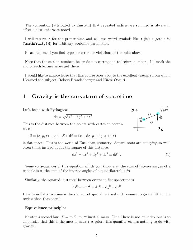
Let’s begin with Pythagoras:

ds =√

dx2 + dy2 + dz2

This is the distance between the points with cartesian coordi-nates

~x = (x, y, z) and ~x+ d~x = (x+ dx, y + dy, z + dz)

in flat space. This is the world of Euclidean geometry. Square roots are annoying so we’lloften think instead about the square of this distance:

ds2 = dx2 + dy2 + dz2 ≡ d~x2 . (1)

Some consequences of this equation which you know are: the sum of interior angles of atriangle is π, the sum of the interior angles of a quadrilateral is 2π.

Similarly, the squared ‘distance’ between events in flat spacetime is

ds2 = −dt2 + dx2 + dy2 + dz2

Physics in flat spacetime is the content of special relativity. (I promise to give a little morereview than that soon.)

Equivalence principles

Newton’s second law: ~F = mi~a. mi ≡ inertial mass. (The i here is not an index but is toemphasize that this is the inertial mass.) A priori, this quantity mi has nothing to do withgravity.

5

Newton’s law of gravity: ~Fg = −mg~∇φ. mg ≡ gravitational mass. φ is the gravitational

potential. Its important property for now is that it’s independent of mg.

It’s worth pausing for a moment here to emphasize that this is an amazingly successfulphysical theory which successfully describes the motion of apples, moons, planets, stars,clusters of stars, galaxies, clusters of galaxies... A mysterious observation is that mi = mg

as far as anyone has been able to tell. This observation is left completely unexplained bythis description of the physics.

Experimental tests of mi = mg:

Galileo, Newton (1686): If mi = mg, Newton’s equation reduces to ~a = −~∇φ, independentof m. Roll objects of different inertial masses (ball of iron, ball of wood) down a slope;observe same final velocity.

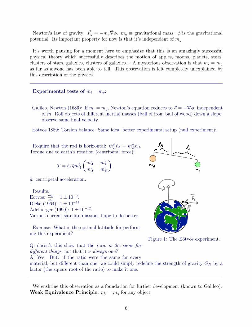
Eotvos 1889: Torsion balance. Same idea, better experimental setup (null experiment):

Figure 1: The Eotvos experiment.

Require that the rod is horizontal: mgA`A = mg

B`B.Torque due to earth’s rotation (centripetal force):

T = `AgmgA

(miA

mgA

− miB

mgB

).

g: centripetal acceleration.

Results:Eotvos: mg

mi= 1± 10−9.

Dicke (1964): 1± 10−11.Adelberger (1990): 1± 10−12.Various current satellite missions hope to do better.

Exercise: What is the optimal latitude for perform-ing this experiment?

Q: doesn’t this show that the ratio is the same fordifferent things, not that it is always one?A: Yes. But: if the ratio were the same for everymaterial, but different than one, we could simply redefine the strength of gravity GN by afactor (the square root of the ratio) to make it one.

We enshrine this observation as a foundation for further development (known to Galileo):Weak Equivalence Principle: mi = mg for any object.

6

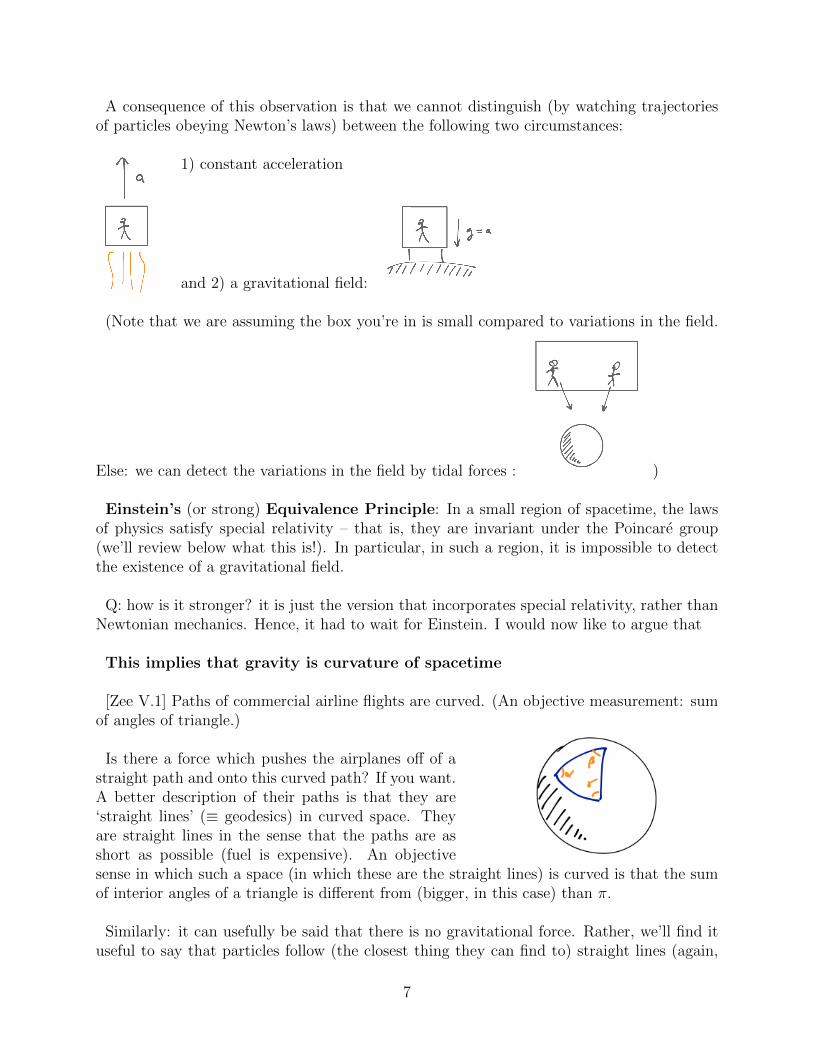
A consequence of this observation is that we cannot distinguish (by watching trajectoriesof particles obeying Newton’s laws) between the following two circumstances:

1) constant acceleration

and 2) a gravitational field:

(Note that we are assuming the box you’re in is small compared to variations in the field.

Else: we can detect the variations in the field by tidal forces : )

Einstein’s (or strong) Equivalence Principle: In a small region of spacetime, the lawsof physics satisfy special relativity – that is, they are invariant under the Poincare group(we’ll review below what this is!). In particular, in such a region, it is impossible to detectthe existence of a gravitational field.

Q: how is it stronger? it is just the version that incorporates special relativity, rather thanNewtonian mechanics. Hence, it had to wait for Einstein. I would now like to argue that

This implies that gravity is curvature of spacetime

[Zee V.1] Paths of commercial airline flights are curved. (An objective measurement: sumof angles of triangle.)

Is there a force which pushes the airplanes off of astraight path and onto this curved path? If you want.A better description of their paths is that they are‘straight lines’ (≡ geodesics) in curved space. Theyare straight lines in the sense that the paths are asshort as possible (fuel is expensive). An objectivesense in which such a space (in which these are the straight lines) is curved is that the sumof interior angles of a triangle is different from (bigger, in this case) than π.

Similarly: it can usefully be said that there is no gravitational force. Rather, we’ll find ituseful to say that particles follow (the closest thing they can find to) straight lines (again,

7

geodesics) in curved spacetime. To explain why this is a good idea, let’s look at someconsequences of the equivalence principle (in either form).

[Zee §V.2] preview of predictions: two of the most striking predictions of the theory we aregoing to study follow (at least qualitatively) directly from the equivalence principle. That is,we can derive these qualitative results from thought experiments. Further, from these tworesults we may conclude that gravity is the curvature of spacetime.

Here is the basic thought experiment setup, using which we’ll discuss four different pro-tocols. Put a person in a box in deep space, no planets or stars around and accelerate ituniformly in a direction we will call ‘up’ with a magnitude g. According to the EEP, theperson experiences this in the same way as earthly gravity.

You can see into the box. The person has a laser gun and some detectors. We’ll have topoints of view on each experiment, and we can learn by comparing them and demandingthat everyone agrees about results that can be compared.

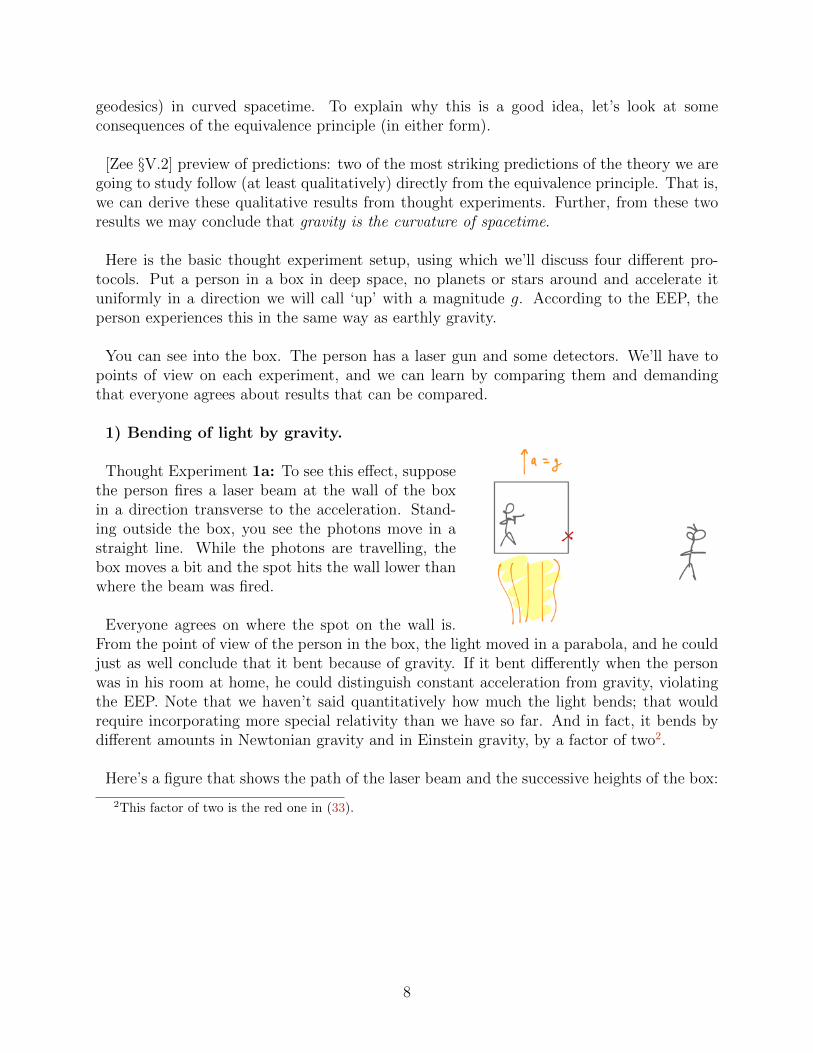
1) Bending of light by gravity.

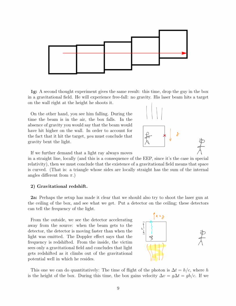
Thought Experiment 1a: To see this effect, supposethe person fires a laser beam at the wall of the boxin a direction transverse to the acceleration. Stand-ing outside the box, you see the photons move in astraight line. While the photons are travelling, thebox moves a bit and the spot hits the wall lower thanwhere the beam was fired.

Everyone agrees on where the spot on the wall is.From the point of view of the person in the box, the light moved in a parabola, and he couldjust as well conclude that it bent because of gravity. If it bent differently when the personwas in his room at home, he could distinguish constant acceleration from gravity, violatingthe EEP. Note that we haven’t said quantitatively how much the light bends; that wouldrequire incorporating more special relativity than we have so far. And in fact, it bends bydifferent amounts in Newtonian gravity and in Einstein gravity, by a factor of two2.

Here’s a figure that shows the path of the laser beam and the successive heights of the box:

2This factor of two is the red one in (33).

8

1g: A second thought experiment gives the same result: this time, drop the guy in the boxin a gravitational field. He will experience free-fall: no gravity. His laser beam hits a targeton the wall right at the height he shoots it.

On the other hand, you see him falling. During thetime the beam is in the air, the box falls. In theabsence of gravity you would say that the beam wouldhave hit higher on the wall. In order to account forthe fact that it hit the target, you must conclude thatgravity bent the light.

If we further demand that a light ray always movesin a straight line, locally (and this is a consequence of the EEP, since it’s the case in specialrelativity), then we must conclude that the existence of a gravitational field means that spaceis curved. (That is: a triangle whose sides are locally straight has the sum of the internalangles different from π.)

2) Gravitational redshift.

2a: Perhaps the setup has made it clear that we should also try to shoot the laser gun atthe ceiling of the box, and see what we get. Put a detector on the ceiling; these detectorscan tell the frequency of the light.

From the outside, we see the detector acceleratingaway from the source: when the beam gets to thedetector, the detector is moving faster than when thelight was emitted. The Doppler effect says that thefrequency is redshifted. From the inside, the victimsees only a gravitational field and concludes that lightgets redshifted as it climbs out of the gravitationalpotential well in which he resides.

This one we can do quantitatively: The time of flight of the photon is ∆t = h/c, where his the height of the box. During this time, the box gains velocity ∆v = g∆t = gh/c. If we

9

suppose a small acceleration, gh/c c, we don’t need the fancy SR Doppler formula (forwhich see Zee §1.3), rather:

ωdetector − ωsource

ωsource

=∆v

c=gh/c

c=gh

c2= −φdetector − φsource

c2

Here ∆φ is the change in gravitational potential between top and bottom of the box.

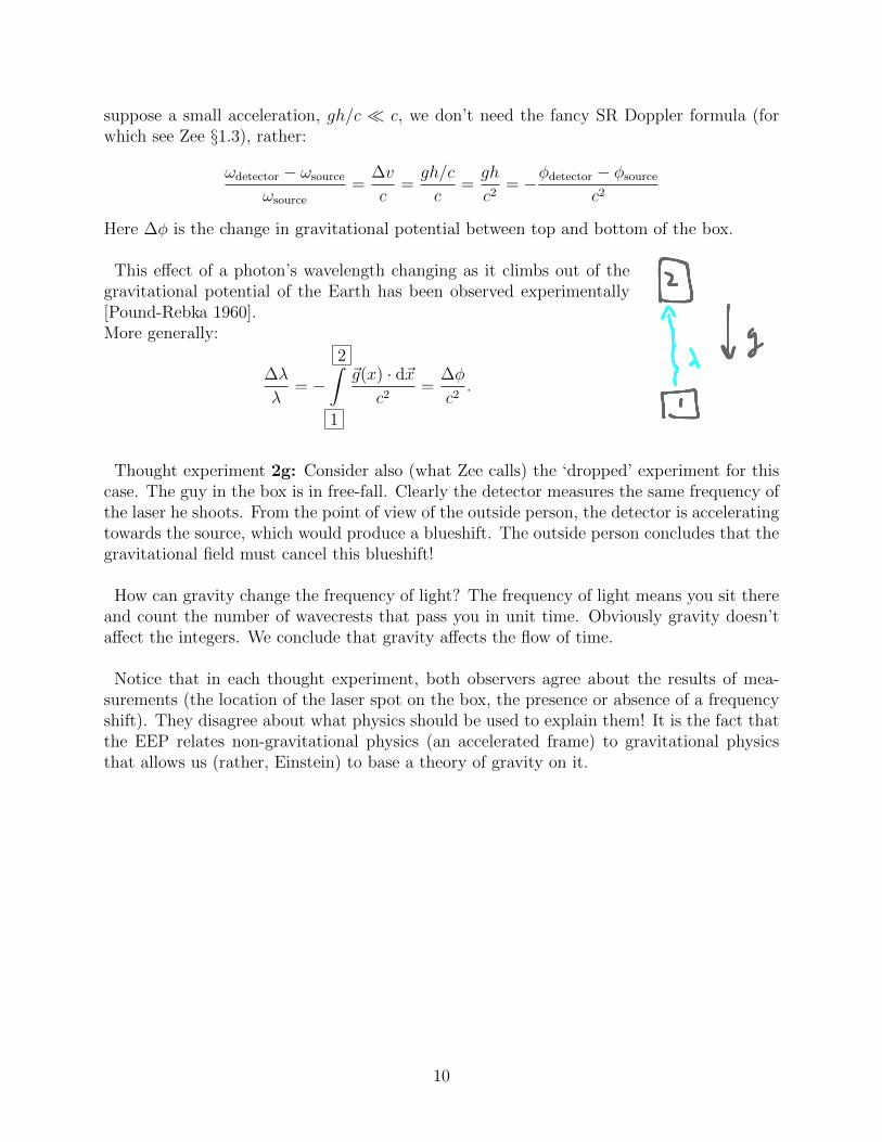
This effect of a photon’s wavelength changing as it climbs out of thegravitational potential of the Earth has been observed experimentally[Pound-Rebka 1960].More generally:

∆λ

λ= −

2∫1

~g(x) · d~xc2

=∆φ

c2.

Thought experiment 2g: Consider also (what Zee calls) the ‘dropped’ experiment for thiscase. The guy in the box is in free-fall. Clearly the detector measures the same frequency ofthe laser he shoots. From the point of view of the outside person, the detector is acceleratingtowards the source, which would produce a blueshift. The outside person concludes that thegravitational field must cancel this blueshift!

How can gravity change the frequency of light? The frequency of light means you sit thereand count the number of wavecrests that pass you in unit time. Obviously gravity doesn’taffect the integers. We conclude that gravity affects the flow of time.

Notice that in each thought experiment, both observers agree about the results of mea-surements (the location of the laser spot on the box, the presence or absence of a frequencyshift). They disagree about what physics should be used to explain them! It is the fact thatthe EEP relates non-gravitational physics (an accelerated frame) to gravitational physicsthat allows us (rather, Einstein) to base a theory of gravity on it.

10

Actually: once we agree that locally physics is relativistically invariant, a Lorentz boostrelates the redshift to the bending.

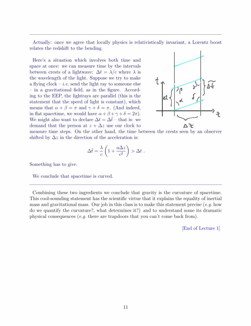
Here’s a situation which involves both time andspace at once: we can measure time by the intervalsbetween crests of a lightwave: ∆t = λ/c where λ isthe wavelength of the light. Suppose we try to makea flying clock – i.e. send the light ray to someone else– in a gravitational field, as in the figure. Accord-ing to the EEP, the lightrays are parallel (this is thestatement that the speed of light is constant), whichmeans that α + β = π and γ + δ = π. (And indeed,in flat spacetime, we would have α+β+ γ+ δ = 2π).We might also want to declare ∆t = ∆t – that is: wedemand that the person at z + ∆z use our clock tomeasure time steps. On the other hand, the time between the crests seen by an observershifted by ∆z in the direction of the acceleration is:

∆t =λ

c

(1 +

a∆z

c2

)> ∆t .

Something has to give.

We conclude that spacetime is curved.

Combining these two ingredients we conclude that gravity is the curvature of spacetime.This cool-sounding statement has the scientific virtue that it explains the equality of inertialmass and gravitational mass. Our job in this class is to make this statement precise (e.g. howdo we quantify the curvature?, what determines it?) and to understand some its dramaticphysical consequences (e.g. there are trapdoors that you can’t come back from).

[End of Lecture 1]

11

Conceptual context and framework of GR

Place of GR in physics:

Classical, Newtonian dynamics with Newtonian gravity

⊂ special relativity + Newtonian gravity (?)

⊂ GR

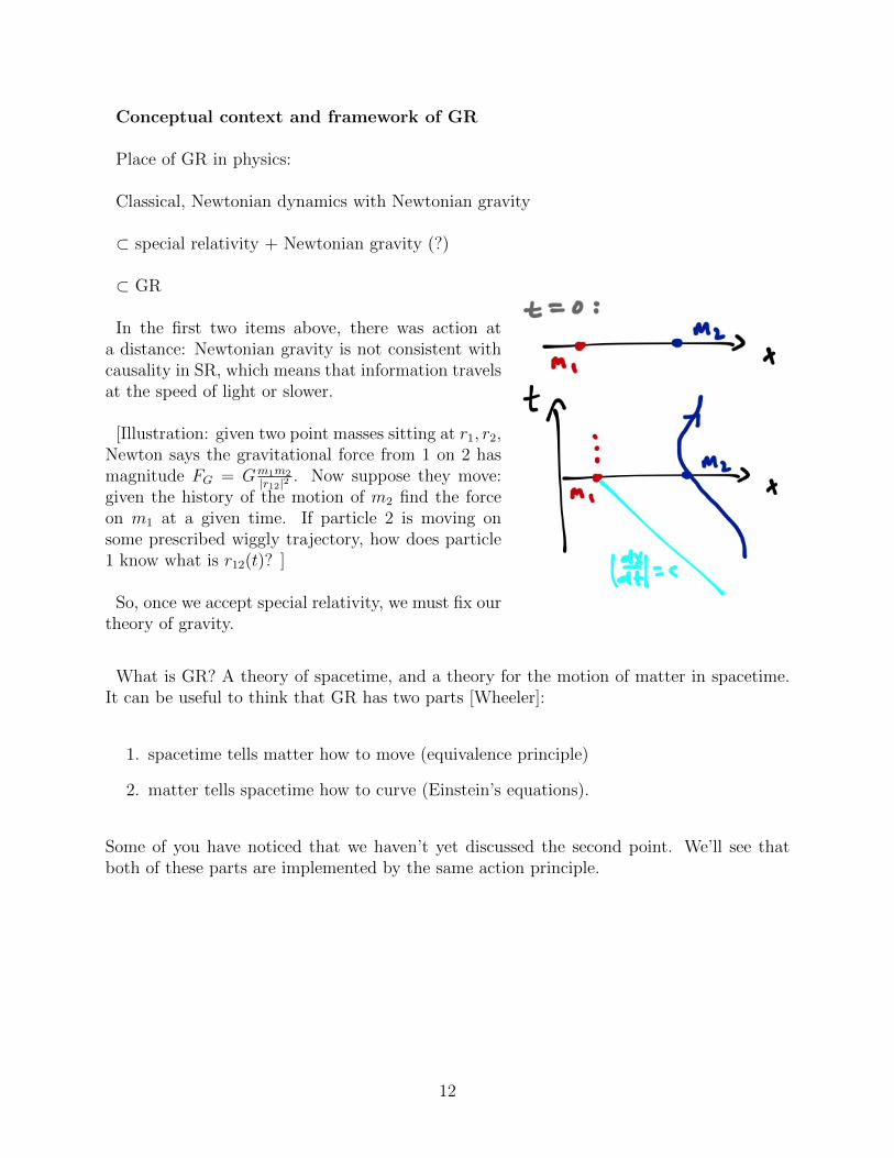
In the first two items above, there was action ata distance: Newtonian gravity is not consistent withcausality in SR, which means that information travelsat the speed of light or slower.

[Illustration: given two point masses sitting at r1, r2,Newton says the gravitational force from 1 on 2 hasmagnitude FG = Gm1m2

|r12|2 . Now suppose they move:given the history of the motion of m2 find the forceon m1 at a given time. If particle 2 is moving onsome prescribed wiggly trajectory, how does particle1 know what is r12(t)? ]

So, once we accept special relativity, we must fix ourtheory of gravity.

What is GR? A theory of spacetime, and a theory for the motion of matter in spacetime.It can be useful to think that GR has two parts [Wheeler]:

1. spacetime tells matter how to move (equivalence principle)

2. matter tells spacetime how to curve (Einstein’s equations).

Some of you have noticed that we haven’t yet discussed the second point. We’ll see thatboth of these parts are implemented by the same action principle.

12

2 Euclidean geometry and special relativity

Special relativity is summarized well in this document – dripping with hindsight.

2.1 Euclidean geometry and Newton’s laws

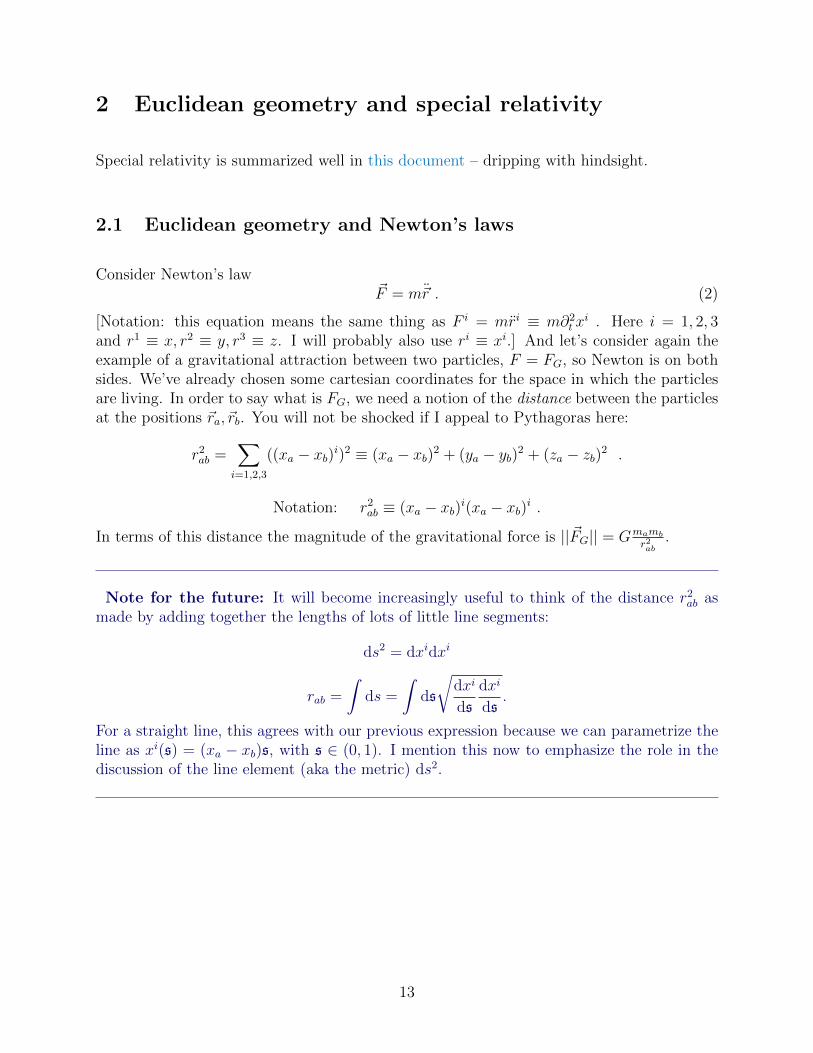
Consider Newton’s law~F = m~r . (2)

[Notation: this equation means the same thing as F i = mri ≡ m∂2t x

i . Here i = 1, 2, 3and r1 ≡ x, r2 ≡ y, r3 ≡ z. I will probably also use ri ≡ xi.] And let’s consider again theexample of a gravitational attraction between two particles, F = FG, so Newton is on bothsides. We’ve already chosen some cartesian coordinates for the space in which the particlesare living. In order to say what is FG, we need a notion of the distance between the particlesat the positions ~ra, ~rb. You will not be shocked if I appeal to Pythagoras here:

r2ab =

∑i=1,2,3

((xa − xb)i)2 ≡ (xa − xb)2 + (ya − yb)2 + (za − zb)2 .

Notation: r2ab ≡ (xa − xb)i(xa − xb)i .

In terms of this distance the magnitude of the gravitational force is ||~FG|| = Gmambr2ab

.

Note for the future: It will become increasingly useful to think of the distance r2ab as

made by adding together the lengths of lots of little line segments:

ds2 = dxidxi

rab =

∫ds =

∫ds

√dxi

ds

dxi

ds.

For a straight line, this agrees with our previous expression because we can parametrize theline as xi(s) = (xa − xb)s, with s ∈ (0, 1). I mention this now to emphasize the role in thediscussion of the line element (aka the metric) ds2.

13

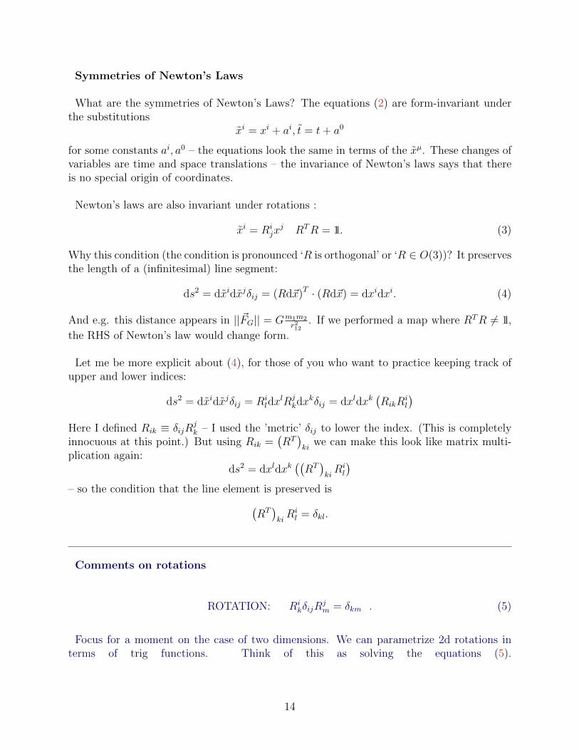
Symmetries of Newton’s Laws

What are the symmetries of Newton’s Laws? The equations (2) are form-invariant underthe substitutions

xi = xi + ai, t = t+ a0

for some constants ai, a0 – the equations look the same in terms of the xµ. These changes ofvariables are time and space translations – the invariance of Newton’s laws says that thereis no special origin of coordinates.

Newton’s laws are also invariant under rotations :

xi = Rijxj RTR = 1. (3)

Why this condition (the condition is pronounced ‘R is orthogonal’ or ‘R ∈ O(3))? It preservesthe length of a (infinitesimal) line segment:

ds2 = dxidxjδij = (Rd~x)T · (Rd~x) = dxidxi. (4)

And e.g. this distance appears in ||~FG|| = Gm1m2

r212

. If we performed a map where RTR 6= 1,

the RHS of Newton’s law would change form.

Let me be more explicit about (4), for those of you who want to practice keeping track ofupper and lower indices:

ds2 = dxidxjδij = Rildx

lRjkdx

kδij = dxldxk(RikR

il

)Here I defined Rik ≡ δijR

jk – I used the ’metric’ δij to lower the index. (This is completely

innocuous at this point.) But using Rik =(RT)ki

we can make this look like matrix multi-plication again:

ds2 = dxldxk((RT)kiRil

)– so the condition that the line element is preserved is(

RT)kiRil = δkl.

Comments on rotations

ROTATION: RikδijR

jm = δkm . (5)

Focus for a moment on the case of two dimensions. We can parametrize 2d rotations interms of trig functions. Think of this as solving the equations (5).

14

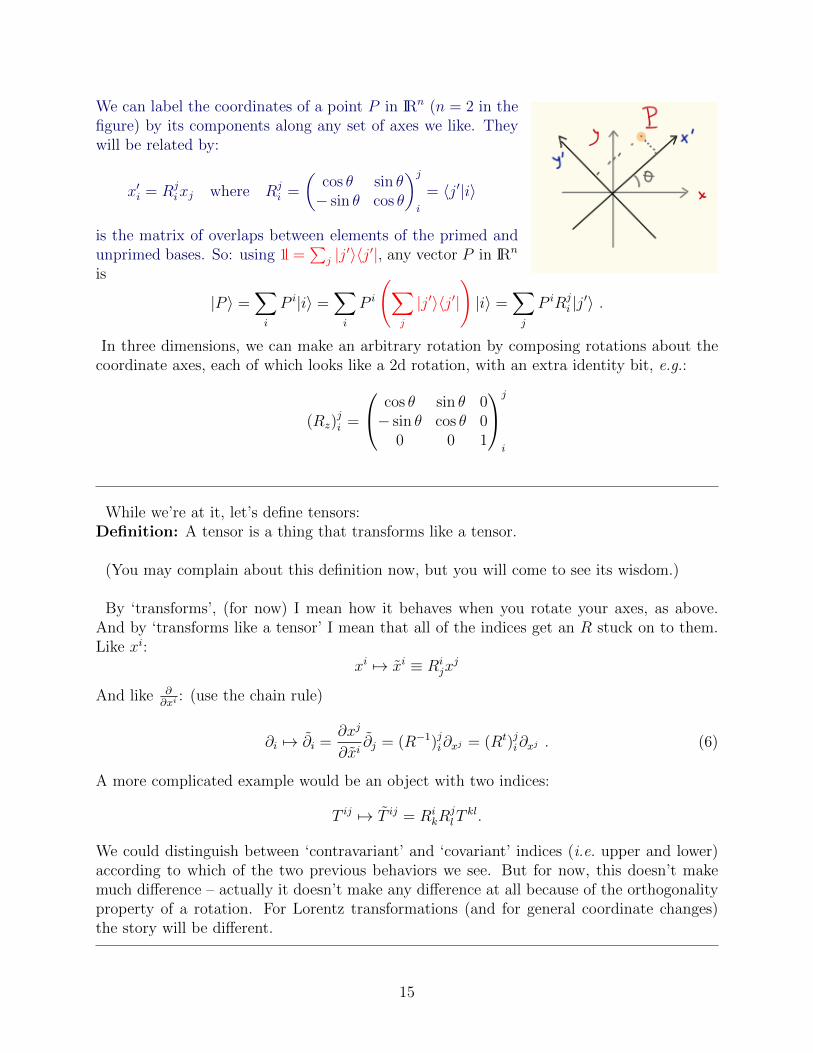
We can label the coordinates of a point P in IRn (n = 2 in thefigure) by its components along any set of axes we like. Theywill be related by:

x′i = Rjixj where Rj

i =

(cos θ sin θ− sin θ cos θ

)ji

= 〈j′|i〉

is the matrix of overlaps between elements of the primed andunprimed bases. So: using 1 =

∑j |j′〉〈j′|, any vector P in IRn

is

|P 〉 =∑i

P i|i〉 =∑i

P i

(∑j

|j′〉〈j′|

)|i〉 =

∑j

P iRji |j′〉 .

In three dimensions, we can make an arbitrary rotation by composing rotations about thecoordinate axes, each of which looks like a 2d rotation, with an extra identity bit, e.g.:

(Rz)ji =

cos θ sin θ 0− sin θ cos θ 0

0 0 1

j

i

While we’re at it, let’s define tensors:Definition: A tensor is a thing that transforms like a tensor.

(You may complain about this definition now, but you will come to see its wisdom.)

By ‘transforms’, (for now) I mean how it behaves when you rotate your axes, as above.And by ‘transforms like a tensor’ I mean that all of the indices get an R stuck on to them.Like xi:

xi 7→ xi ≡ Rijxj

And like ∂∂xi

: (use the chain rule)

∂i 7→ ∂i =∂xj

∂xi∂j = (R−1)ji∂xj = (Rt)ji∂xj . (6)

A more complicated example would be an object with two indices:

T ij 7→ T ij = RikR

jlT

kl.

We could distinguish between ‘contravariant’ and ‘covariant’ indices (i.e. upper and lower)according to which of the two previous behaviors we see. But for now, this doesn’t makemuch difference – actually it doesn’t make any difference at all because of the orthogonalityproperty of a rotation. For Lorentz transformations (and for general coordinate changes)the story will be different.

15

Clouds on the horizon: Another symmetry of Newton’s law is the Galilean boost:

xi = xi + vit, t = t. (7)

Newton’s laws are form-invariant under this transformation, too. Notice that there is arather trivial sense in which (7) preserves the length of the infinitesimal interval:

ds2 = dxidxjδij = dxidxi

since time simply does not appear – it’s a different kind of thing.

The preceding symmetry transformations comprise the Galilei group: it has ten generators(time translations, 3 spatial translations, 3 rotations and 3 Galilean boosts). It’s rightfullycalled that given how vigorously Galileo emphasized the point that physics looks the same incoordinate systems related by (7). If you haven’t read his diatribe on this with the butterfliesflying indifferently in every direction, do so at your earliest convenience; it is hilarious. Anexcerpt is here.

2.2 Maxwell versus Galileo and Newton: Maxwell wins

Let’s rediscover the structure of the Lorentz group in the historical way: via the fact thatMaxwell’s equations are not invariant under (7), but rather have Lorentz symmetry.

Maxwell said ...

~∇× ~E +1

c∂t ~B = 0, ~∇ · ~B = 0

~∇× ~B − 1

c∂t ~E = 4π

c~J, ~∇ · ~E = 4πρ (8)

.... and there was light. If you like, these equations are empirical facts. Combining Ampereand Faraday, one learns that (e.g.in vacuum)(

∂2t − c2∇2

)~E = 0

– the solutions are waves moving at the speed c, which is a constant appearing in (8) (whichis measured by doing experiments with capacitors and stuff).

Maxwell’s equations are not inv’t under Gal boosts, which change the speed of light.

They are invariant under the Poincare symmetry. Number of generators is the same asGal: 1 time translation, 3 spatial translations, 3 rotations and 3 (Lorentz!) boosts. The last3 are the ones which distinguish Lorentz from Galileo, but before we get there, we need tograpple with the fact that we are now studying a field theory.

16

A more explicit expression of Maxwell’s equations is:

εijk∂jEk +1

c∂tB

i = 0, ∂iBi = 0

εijk∂jBk −1

c∂tE

i = 4πcJ i, ∂iE

i = 4πρ (9)

Here in writing out the curl:(~∇× ~E

)i

= εijk∂jEk we’ve introduced the useful Levi-Civita

symbol, εijk. It is a totally anti-symmetric object with ε123 = 1. It is a ”pseudo-tensor”:the annoying label ‘pseudo’ is not a weakening qualifier, but rather an additional bit ofinformation about the way it transforms under rotations that include a parity transformation(i.e. those which map a right-handed frame (like xyz) to a left-handed frame (like yxz), andtherefore have detR = −1. For those of you who like names, such transformations are inO(3) but not SO(3).) As you’ll show on the homework, it transforms like

εijk 7→ εijk = ε`mnR`iR

mj R

nk = (detR) εijk.

RTR = 1 =⇒ (detR)2 = 1 =⇒ detR = ±1

If R preserves a right-handed coordinate frame, detR = 1.

Notice by the way that so far I have not attributed any meaning to upper or lower indices.And we can get away with this when our indices are spatial indices and we are only thinkingabout rotations because of (6).

Comment about tensor fields

Here is a comment which may head off some confusions about the first problem set. Theobjects ~E(x, t) and ~B(x, t) are vectors (actually ~B is a pseudovector) at each point in space-time, that is – they are vector fields. We’ve discussed above the rotation properties of vectorsand other tensors; now we have to grapple with transforming a vector at each point in space,while at the same time rotating the space.

The rotation is a relabelling xi = Rijxj, with RijRkj = δik so that lengths are preserved. As

always when thinking about symmetries, it’s easy to get mixed up about active and passivetransformations. The important thing to keep in mind is that we are just relabelling thepoints (and the axes), and the values of the fields at the points are not changed by thisrelabelling. So a scalar field (a field with no indices) transforms as

φ(x) = φ(x).

Notice that φ is a different function of its argument from φ; it differs in exactly such a

way as to undo the relabelling. So it’s NOT true that φ(x)?= φ(x), NOR is it true that

φ(x)?= φ(Rx) which would say the same thing, since R is invertible.

17

A vector field is an arrow at each point in space; when we rotate our labels, we change ouraccounting of the components of the vector at each point, but must ensure that we don’tchange the vector itself. So a vector field transforms like

Ei(x) = RijEj(x).

For a clear discussion of this simple but slippery business3 take a look at page 46 of Zee’sbook.

The statement that ~B is a pseudovector means that it gets an extra minus sign for parity-reversing rotations:

Bi(x) = detRRijBj(x).

To make the Poincare invariance manifest, let’s rewrite Maxwell (8) in better notation:

εµ···∂·F·· = 0, η··∂·Fµ· = 4πjν .

4 Again this is 4 + 4 equations; let’s show that they are the same as (8). Writing them insuch a compact way requires some notation (which was designed for this job, so don’t be tooimpressed yet5).

In terms of Fij ≡ εijkBk (note that Fij = −Fji),

∂jEk − ∂kEj +1

c∂tFjk = 0, εijk∂iFjk = 0

∂iFij −1

c∂tEi = 4π

cJi, ∂iE

i = 4πρ (10)

Introduce x0 = ct. Let Fi0 = −F0i = Ei. F00 = 0. (Note: F has lower indices and theymean something.) With this notation, the first set of equations can be written as

∂µFνρ + ∂νFρµ + ∂ρFµν = 0

better notation: εµνρσ∂νFρσ = 0.

In this notation, the second set is

ηνρ∂νFµρ = 4πjµ (11)

3 Thanks to Michael Gartner for reminding me that this is so simple that it’s actually quite difficult.4A comment about notation: here and in many places below I will refuse to assign names to dummy

indices when they are not required. The ·s indicate the presence of indices which need to be contracted. Ifyou must, imagine that I have given them names, but written them in a font which is too small to see.

5See Feynman vol II §25.6 for a sobering comment on this point.

18

where we’ve packaged the data about the charges into a collection of four objects:

j0 ≡ −cρ, ji ≡ Ji .

(It is tempting to call this a four-vector, but that is a statement about its transformationlaws which remains to be seen. Spoilers: it is in fact a 4-vector.)

Here the quantity

ηνρ ≡

−1 0 0 00 1 0 00 0 1 00 0 0 1

νρ

makes its first appearance in our discussion. At the moment is is just a notational deviceto get the correct relative sign between the ∂tE and the ~∇E terms in the second Maxwellequation.

The statement that the particle current is conserved:

0 =c∂ρ

∂ (ct)+ ~∇ · ~J now looks like 0 = −∂tj0 + ∂iji = ηµν

∂

∂xµjν ≡ ∂µjµ ≡ ∂µj

µ. (12)

This was our first meaningful raising of an index. Consistency of Maxwell’s equations requiresthe equation :

0 = ∂µ∂νFµν .

It is called the ‘Bianchi identity’ – ‘identity’ because it is identically true by antisymmetryof derivatives (as long as F is smooth).

Symmetries of Maxwell equations

Consider the substitutionxµ 7→ xµ = Λµ

νxν ,

under which∂µ 7→ ∂µ, with ∂µ = Λν

µ∂ν .

At the moment Λ is a general 4× 4 matrix of constants.

If we declare that everything in sight transforms like a tensor under these transformations– that is if:

Fµν(x) 7→ Fµν(x) , Fµν(x) = ΛρµΛσ

ν Fρσ(x)

jµ(x) 7→ jµ(x) , jµ(x) = Λνµjν(x)

then Maxwell’s equations in the new variables are

(det Λ)Λµκεκνρσ∂νFρσ = 0

ηνρΛκν ∂κΛ

σµΛλ

ρFσλ = 4πΛℵµJℵ.

19

6 Assume Λ is invertible, so we can strip off a Λ from this equation to get:

ηνρΛκνΛ

λρ ∂κFσλ = 4πJσ.

This looks like the original equation (11) in the new variables if Λ satisfies

Λκνη

νρΛλρ = ηκλ (13)

– this is a condition on the collection of numbers Λ:

ΛTηΛ = η

which is pronounced ‘Λ is in O(3, 1)’ (the numbers are the numbers of +1s and −1s in thequadratic form η). Note the very strong analogy with (5); the only difference is that thetransformation preserves η rather than δ. The ordinary rotation is a special case of Λ withΛ0µ = 0,Λµ

0 = 0. The point of the notation we’ve constructed here is to push this analogy infront of our faces.

Are these the right transformation laws for Fµν? I will say two things in their defense.First, the rule Fµν = Λρ

µΛσν Fρσ follows immediately if the vector potential Aµ is a vector field

andFµν = ∂µAν − ∂νAµ .

Perhaps more convincingly, one can derive pieces of these transformation rules for ~E and~B by considering the transformations of the charge and current densities that source them.This is described well in the E&M book by Purcell and I will not repeat it.

You might worry further that the transformation laws of jµ are determined by already bythe transformation laws of xµ – e.g. consider the case that the charges are point particles –we don’t get to pick the transformation law. We’ll see below that the rule above is correct– jµ really is a 4-vector.

A word of nomenclature: the Lorentz group is the group of Λµν above, isomorphic to

SO(3, 1). It is a subgroup of the Poincare group, which includes also spacetime transla-tions, xµ 7→ Λµ

νxν + aν .

Lorentz transformations of charge and current density

Here is a simple way to explain the Lorentz transformation law for the current. Considera bunch of charge Q in a (small) volume V moving with velocity ~u. The charge and currentdensity are

ρ = Q/V, ~J = ρ~u.

6Two comments: (1) Already we’re running out of letters! Notice that the only meaningful index on theBHS of this equation is µ – all the others are dummies. (2) Notice that the derivative on the RHS is actingonly on the F – everything else is constants.

20

In the rest frame, ~u0 = 0, ρ0 ≡ QV0

. The charge is a scalar, but the volume is contracted in

the direction of motion: V = 1γV0 =

√1− u2/c2V0

=⇒ ρ = ρ0γ, ~J = ρ0γ~u .

But this means exactly thatJµ = (ρ0γc, ρ0γ~u)µ

is a 4-vector.

(In lecture, I punted the discussion in the following paragraph until we construct worldlineactions.) We’re going to have to think about currents made of individual particles, and we’lldo this using an action in the next section. But let’s think in a little more detail aboutthe form of the current four-vector for a single point particle: Consider a point particle withtrajectory ~x0(t) and charge e. The charge density and current density are only nonzero wherethe particle is:

ρ(t, ~x) = eδ(3)(~x− ~x0(t)) (14)

~j(t, ~x) = eδ(3)(~x− ~x0(t))d~x0

dt(15)

xµ0(t) ≡ (ct, ~x0(t))µ

transforms likexµ 7→ xµ = Λµ

νxν

jµ(x) = eδ(3)(~x− ~x0(t))dxµ0(t)

dt= e

∫ ∞−∞

dt′δ(4)(x− x0(t′))dxµ0dt′

(t′)

using δ(4)(x − x0(t′)) = δ(3)(~x − ~x0(t′))δ(x0 − ct′). Since we can choose whatever dummyintegration variable we want,

jµ = e

∫ ∞−∞

dsδ(4)(x− x0(s))dxµ0ds

(s) (16)

is manifestly a Lorentz 4-vector – it transforms the same way as xµ.

2.3 Minkowski spacetime

Let’s collect the pieces here. We have discovered Minkowski spacetime, the stage on whichspecial relativity happens. This spacetime has convenient global coordinates xµ = (ct, xi)µ.µ = 0, 1, 2, 3, i = 1, 2, 3 or x, y, z.

Our labels on points in this space change under a Lorentz transformation by xµ 7→ xµ =Λµνx

ν . It’s not so weird; we just have to get used to the fact that our time coordinate is aprovincial notion of slow-moving creatures such as ourselves.

21

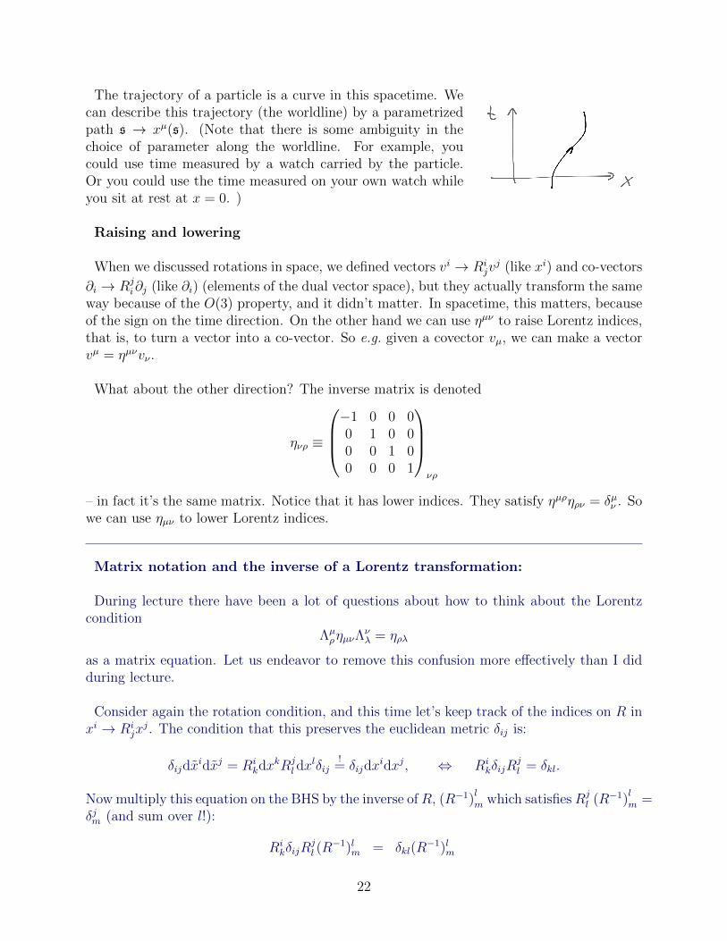
The trajectory of a particle is a curve in this spacetime. Wecan describe this trajectory (the worldline) by a parametrizedpath s → xµ(s). (Note that there is some ambiguity in thechoice of parameter along the worldline. For example, youcould use time measured by a watch carried by the particle.Or you could use the time measured on your own watch whileyou sit at rest at x = 0. )

Raising and lowering

When we discussed rotations in space, we defined vectors vi → Rijvj (like xi) and co-vectors

∂i → Rji∂j (like ∂i) (elements of the dual vector space), but they actually transform the same

way because of the O(3) property, and it didn’t matter. In spacetime, this matters, becauseof the sign on the time direction. On the other hand we can use ηµν to raise Lorentz indices,that is, to turn a vector into a co-vector. So e.g. given a covector vµ, we can make a vectorvµ = ηµνvν .

What about the other direction? The inverse matrix is denoted

ηνρ ≡

−1 0 0 00 1 0 00 0 1 00 0 0 1

νρ

– in fact it’s the same matrix. Notice that it has lower indices. They satisfy ηµρηρν = δµν . Sowe can use ηµν to lower Lorentz indices.

Matrix notation and the inverse of a Lorentz transformation:

During lecture there have been a lot of questions about how to think about the Lorentzcondition

ΛµρηµνΛ

νλ = ηρλ

as a matrix equation. Let us endeavor to remove this confusion more effectively than I didduring lecture.

Consider again the rotation condition, and this time let’s keep track of the indices on R inxi → Ri

jxj. The condition that this preserves the euclidean metric δij is:

δijdxidxj = Ri

kdxkRj

l dxlδij

!= δijdx

idxj, ⇔ RikδijR

jl = δkl.

Now multiply this equation on the BHS by the inverse ofR, (R−1)lm which satisfiesRj

l (R−1)lm =

δjm (and sum over l!):

RikδijR

jl (R

−1)lm = δkl(R−1)lm

22

Rikδim = δkl(R

−1)lm,δklRi

kδim = (R−1)lm, (17)

This is an equation for the inverse of R in terms of R. The LHS here is what we mean byRT if we keep track of up and down.

The same thing for Lorentz transformations (with Λ−1 defined to satisfy Λνσ (Λ−1)

σρ = δνρ)

gives:

ΛµρηµνΛ

νσ = ηρσ

ΛµρηµνΛ

νσ

(Λ−1

)σρ

= ηρσ(Λ−1

)σρ

Λµρηµρ = ηρσ

(Λ−1

)σρ

ηρσΛµρηµρ =

(Λ−1

)σρ

(18)

This is an expression for the inverse of a Lorentz transformation in terms of Λ itself and theMinkowski metric. This reduces to the expression above in the case when Λ is a rotation,which doesn’t mix in the time coordinate, and involves some extra minus signs when it does.

Proper length.

It will be useful to introduce a notion of the proper length of the path xµ(s) with s ∈ [s1, s2].

First, if v and w are two 4-vectors – meaning that they transform under Lorentz transfor-mations like

v 7→ v = Λv, i.e. vµ 7→ vµ = Λµνv

ν = wµvµ = wµvµ.

– then we can make a number out of them by

v · w ≡ −v0w0 + ~v · ~w = ηµνwµwν

with (again)

ηνρ ≡

−1 0 0 00 1 0 00 0 1 00 0 0 1

νρ

.

This number has the virtue that it is invariant under Lorentz transformations by the definingproperty (13). A special case is the proper length of a 4-vector ||v ||2 ≡ v · v = ηµνv

µvν .

A good example of a 4-vector whose proper length we might want to study is the tangentvector to a particle worldline:

dxµ

ds.

Tangent vectors to trajectories of particles that move slower than light have a negativeproper length-squared (with our signature convention). For example, a particle which just

23

sits at x = 0 and we can take t(s) = s, x(s) = 0, so we have

|| dxµ

ds||2 = −dt

dt

2

= −1 < 0 .

(Notice that changing the parametrization s will rescale this quantity, but will not change itssign.) Exercise: Show that by a Lorentz boost you cannot change the sign of this quantity.

Light moves at the speed of light. A light ray headed in the x direction satisfies x = ct,can be parametrized as t(s) = s, x(s) = cs. So the proper length of a segment of its path(proportional to the proper length of a tangent vector) is

ds2|lightray = −c2dt2 + dx2 = 0

(factors of c briefly restored). Rotating the direction in space doesn’t change this fact.Proper time does not pass along a light ray.

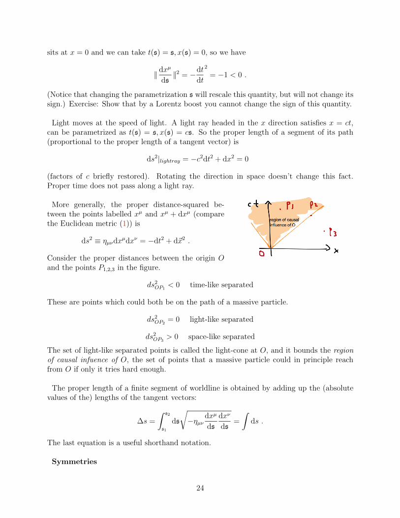
More generally, the proper distance-squared be-tween the points labelled xµ and xµ + dxµ (comparethe Euclidean metric (1)) is

ds2 ≡ ηµνdxµdxν = −dt2 + d~x2 .

Consider the proper distances between the origin Oand the points P1,2,3 in the figure.

ds2OP1

< 0 time-like separated

These are points which could both be on the path of a massive particle.

ds2OP2

= 0 light-like separated

ds2OP3

> 0 space-like separated

The set of light-like separated points is called the light-cone at O, and it bounds the regionof causal infuence of O, the set of points that a massive particle could in principle reachfrom O if only it tries hard enough.

The proper length of a finite segment of worldline is obtained by adding up the (absolutevalues of the) lengths of the tangent vectors:

∆s =

∫ s2

s1

ds

√−ηµν

dxµ

ds

dxν

ds=

∫ds .

The last equation is a useful shorthand notation.

Symmetries

24

The Galilean boost (7) does not preserve the form of the Minkowski line element. Consider1d for simplicity:

dt2 − d~x2 = dt2 − d~x2 − 2d~x · ~vdt− v2dt2 6= dt2 − dx2.

It does not even preserve the form of the lightcone.

Lorentz boosts instead:xµ = Λµ

νxν .

ROTATION: RikδijR

jm = δkm .

BOOST: ΛµρηµνΛ

νλ = ηρλ .

[End of Lecture 2]

Unpacking the Lorentz boost

Consider D = 1 + 1 spacetime dimensions7. Just as we can parameterize a rotation intwo dimensions in terms of trig functions because of the identity cos2 θ + sin2 θ = 1, we canparametrize a D = 1+1 boost in terms of hyperbolic trig functions, with cosh2 Υ−sinh2 Υ =1.

The D = 1 + 1 Minkowski metric is ηµν =

(−1 00 1

)µν

.

The condition that a boost Λµν preserve the Minkowski line element is

Λρµη

µνΛσν = ηρσ . (19)

A solution of this equation is of the form

Λµν =

(cosh Υ sinh Υsinh Υ cosh Υ

)µν

.

from which (19) follows by the hyperbolig trig identity.

(The quantity parameterizing the boost Υ is called the rapidity. As you can see from thetop row of the equation xµ = Λµ

νxν , the rapidity is related to the velocity of the new frame

by tanh Υ = uc.)

7Notice the notation: I will try to be consistent about writing the number of dimensions of spacetime inthis format; if I just say 3 dimensions, I mean space dimensions.

25

A useful and memorable form of the above transformation matrix between frames withrelative x-velocity u (now with the y and z directions going along for the ride) is:

Λ =

γ u

cγ 0 0

ucγ γ 0 00 0 1 00 0 0 1

, γ ≡ 1√1− u2/c2

(= cosh Υ). (20)

So in particular,

x =

ctxyz

7→ x = Λx =

γ(ct+ u

cx)

γ(x+ u

cct)

yz

.

Review of relativistic dynamics of a particle

So far we’ve introduced this machinery for doing Lorentz transformations, but haven’t saidanything about using it to study the dynamics of particles. We’ll rederive this from an actionprinciple soon, but let’s remind ourselves.

Notice that there are two different things we might mean by velocity.

• The coordinate velocity in a particular inertial frame is

~u =d~x

dt7→ ~u =

~u− ~v1− uv

c2

You can verify this transformation law using the Lorentz transformation above.

• The proper velocity is defined as follows. The proper time along an interval of particletrajectory is defined as dτ in:

ds2 = −c2dt2 + d~x2 ≡ −c2dτ 2

– the minus sign makes dτ 2 positive. Notice that(dτ

dt

)2

= 1− u2/c2 =⇒ dτ

dt=√

1− u2/c2 = 1/γu.

The proper velocity is thend~x

ds= γu~u.

Since dxµ = (cdt, d~x)µ is a 4-vector, so is the proper velocity, 1dτ

dxµ = (γc, γ~u)µ.

26

To paraphrase David Griffiths, if you’re on an airplane, the coordinate velocity in the restframe of the ground is the one you care about if you want to know whether you’ll have timeto go running when you arrive; the proper velocity is the one you care about if you arecalculating when you’ll have to go to the bathroom.

So objects of the form a0(γc, γ~u)µ (where a0 is a scalar quantity) are 4-vectors. 8 A usefulnotion of 4-momentum is

pµ = m0dxµ

dτ= (m0γc,m0γ~v)µ

which is a 4-vector. If this 4-momentum is conserved in one frame dpµ

dτ= 0 then dpµ

dτ= 0

in another frame. (This is not true of m0 times the coordinate velocity.) And its timecomponent is p0 = m0γc, that is, E = p0c = m(v)c2. In the rest frame v = 0, this isE0 = m0c

2.

The relativistic Newton laws are then:

~F =d

dt~p still

~p = m~v still

but m = m(v) = m0γ.

Let’s check that energy E = m(v)c2 is conserved according to these laws. A force does thefollowing work on our particle:

dE

dt= ~F · ~v =

d

dt(m(v)~v) · v

2m ·(

d

dt

(m(v)c2

)= ~v · d

dt(m~v)

)c22m

dm

dt= 2m~v · d

dt(m~v)

d

dt

(m2c2

)=

d

dt(m~v)2 =⇒ (mc)2 = (mv)2 + const.

v = 0 : m2(v = 0)c2 ≡ m0c2 = const

=⇒ m(v)2c2 = m(v)2v2 +m20c

2 =⇒ m(v) =m0√1− v2

c2

= m0γv.

8We have already seen an example of something of this form in our discussion of the charge current inMaxwell’s equations:

jµ = ρ0 (γc, γ~u)µ

where ρ0 is the charge density in the rest frame of the charge. So now you believe me that jµ really is a4-vector.

27

Let me emphasize that the reason to go through all this trouble worrying about how thingstransform (and making a notation which makes it manifest) is because we want to buildphysical theories with these symmetries. A way to guarantee this is to make actions whichare invariant (next). But by construction any object we make out of tensors where allthe indices are contracted is Lorentz invariant. (A similar strategy will work for generalcoordinate invariance later.)

2.4 Non-inertial frames versus gravitational fields

[Landau-Lifshitz volume 2, §82] Now that we understand special relativity, we can make amore concise statement of the EEP:

It says that locally spacetime looks like Minkowski spacetime. Let’s think a bit about thatdangerous word ‘locally’.

It is crucial to understand the difference between an actual gravitational field and justusing bad (meaning, non-inertial) coordinates for a situation with no field. It is a slipperything: consider the transformation to a uniformly accelerating frame9:

x = x− 1

2at2, t = t.

You could imagine figuring out dx = dx−atdt, dt = dt and plugging this into ds2 = ds2Mink to

derive the line element experienced by someone in Minkowski space using these non-inertialcoordinates. This could be a useful thing – e.g. you could use it to derive inertial forces (likethe centrifugal and coriolis forces; see problem set 3). You’ll get something that looks like

ds2Mink = gµν(x)dxµdxν .

It will no longer be a sum of squares; there will be cross terms proportional to dxdt = dtdx,and the coefficients gµν will depend on the new coordinates. You can get some prettycomplicated things this way. But they are still just Minkowski space.

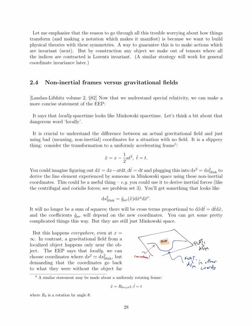
But this happens everywhere, even at x =∞. In contrast, a gravitational field from alocalized object happens only near the ob-ject. The EEP says that locally, we canchoose coordinates where ds2 ' ds2

Mink, butdemanding that the coordinates go backto what they were without the object far

9 A similar statement may be made about a uniformly rotating frame:

x = Rθ=ωtx, t = t

where Rθ is a rotation by angle θ.

28

away forces something to happen in be-tween. That something is curvature.

Evidence that there is room for using gµν as dynamical variables (that is, that not everysuch collection of functions can be obtained by a coordinate transformation) comes fromthe following counting: this is a collection of functions; in D = 3 + 1 there are 4 diagonalentries (µ = ν) and because of the symmetry dxµdxν = dxνdxµ there are 4·3

2= 6 off-diagonal

(µ 6= ν) entries, so 10 altogether. But an arbitrary coordinate transformation xµ → xµ(x) isonly 4 functions. So there is room for something good to happen.

3 Actions

So maybe (I hope) I’ve convinced you that it’s a good idea to describe gravitational inter-actions by letting the metric on spacetime be a dynamical variable. To figure out how todo this, it will be very useful to be able to construct action functionals for the stuff that wewant to interact gravitationally. In case you don’t remember, the action is a single numberassociated to every configuration of the system (i.e. a functional) whose extremization givesthe equations of motion.

As Zee says, physics is where the action is. It is also usually true that the action is wherethe physics is10.

3.1 Reminder about Calculus of Variations

We are going to need to think about functionals – things that eat functions and give numbers– and how they vary as we vary their arguments. We’ll begin by thinking about functionsof one variable, which let’s think of as the (1d) position of a particle as a function of time,x(t).

The basic equation of the calculus of variations is:

δx(t)

δx(s)= δ(t− s) . (21)

From this rule and integration by parts we can get everything we need. For example, let’sask how does the potential term in the action SV [x] =

∫dtV (x(t)) vary if we vary the path

10The exceptions come from the path integral measure in quantum mechanics. A story for a different day.

29

of the particle. Using the chain rule, we have:

δSV =

∫dsδx(s)

δ∫dtV (x(t))

δx(s)=

∫dsδx(s)

∫dt∂xV (x(t))δ(t− s) =

∫dtδx(t)∂xV (x(t)).

(22)We could rewrite this information as :

δ

δx(s)

∫dtV (x(t)) = V ′(x(s)).

[picture from Herman Verlinde]

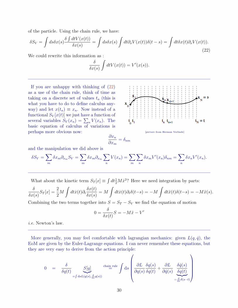
If you are unhappy with thinking of (22)as a use of the chain rule, think of time astaking on a discrete set of values tn (this iswhat you have to do to define calculus any-way) and let x(tn) ≡ xn. Now instead of afunctional SV [x(t)] we just have a function ofseveral variables SV (xn) =

∑n V (xn). The

basic equation of calculus of variations isperhaps more obvious now:

∂xn∂xm

= δnm

and the manipulation we did above is

δSV =∑m

δxm∂xmSV =∑m

δxm∂xm∑n

V (xn) =∑m

∑n

δxmV′(xn)δnm =

∑n

δxnV′(xn).

What about the kinetic term ST [x] ≡∫dt1

2Mx2? Here we need integration by parts:

δ

δx(s)ST [x] =

2

2M

∫dtx(t)∂t

δx(t)

δx(s)= M

∫dtx(t)∂tδ(t−s) = −M

∫dtx(t)δ(t−s) = −Mx(s).

Combining the two terms together into S = ST − SV we find the equation of motion

0 =δ

δx(t)S = −Mx− V ′

i.e. Newton’s law.

More generally, you may feel comfortable with lagrangian mechanics: given L(q, q), theEoM are given by the Euler-Lagrange equations. I can never remember these equations, butthey are very easy to derive from the action principle:

0 =δ

δq(t)S[q]︸︷︷︸

=∫

dsL(q(s), ddsq(s))

chain rule=

∫ds

∂L

∂q(s)

δq(s)

δq(t)+

∂L

∂q(s)

δq(s)

δq(t)︸ ︷︷ ︸= d

dsδ(s−t)

30

IBP=

∫dsδ(s− t)

(∂L

∂q(s)− d

ds

∂L

∂q(s)

)=

∂L

∂q(t)− d

dt

∂L

∂q(t). (23)

(Notice at the last step that L means L(q(t), q(t)).)

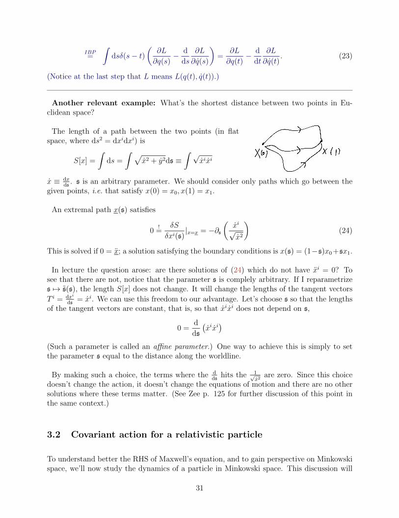
Another relevant example: What’s the shortest distance between two points in Eu-clidean space?

The length of a path between the two points (in flatspace, where ds2 = dxidxi) is

S[x] =

∫ds =

∫ √x2 + y2ds ≡

∫ √xixi

x ≡ dxds

. s is an arbitrary parameter. We should consider only paths which go between thegiven points, i.e. that satisfy x(0) = x0, x(1) = x1.

An extremal path x(s) satisfies

0!

=δS

δxi(s)|x=x = −∂s

(xi√x2

)(24)

This is solved if 0 = x; a solution satisfying the boundary conditions is x(s) = (1−s)x0 +sx1.

In lecture the question arose: are there solutions of (24) which do not have xi = 0? Tosee that there are not, notice that the parameter s is complely arbitrary. If I reparametrizes 7→ s(s), the length S[x] does not change. It will change the lengths of the tangent vectors

T i = dxi

ds= xi. We can use this freedom to our advantage. Let’s choose s so that the lengths

of the tangent vectors are constant, that is, so that xixi does not depend on s,

0 =d

ds

(xixi

)(Such a parameter is called an affine parameter.) One way to achieve this is simply to setthe parameter s equal to the distance along the worldline.

By making such a choice, the terms where the dds

hits the 1√x2

are zero. Since this choicedoesn’t change the action, it doesn’t change the equations of motion and there are no othersolutions where these terms matter. (See Zee p. 125 for further discussion of this point inthe same context.)

3.2 Covariant action for a relativistic particle

To understand better the RHS of Maxwell’s equation, and to gain perspective on Minkowskispace, we’ll now study the dynamics of a particle in Minkowski space. This discussion will

31

be useful for several reasons. We’ll use this kind of action below to understand the motionof particles in curved space. And it will be another encounter with the menace of coordinateinvariance (in D = 0 + 1). In fact, it can be thought of as a version of general relativity inD = 0 + 1.

S[x] = mc2

∫dτ =

∞∫−∞

dsL0 .

L0 = −mc2 dτ

ds= −m

√−(

dx

ds

)2

= −m√−ηµν

dxµ

ds

dxν

ds

What is this quantity? It’s the (Lorentz-invariant) proper time of the worldline, −mc2∫

dτ(ds2 ≡ −c2dτ 2 – the sign is the price we pay for our signature convention where time is theweird one.) in units of the mass. Notice that the object S has dimensions of action; theoverall normalization doesn’t matter in classical physics, which only cares about differencesof action, but it is not a coincidence that it has the same units as ~.

Let xµ ≡ dxµ

ds. The canonical momentum is

pµ ≡∂L0

∂xµ=mcηµν x

ν

√−x2

.

(Beware restoration of cs.)

A useful book-keeping fact: when we differentiate with respect to a covariant vector ∂∂xµ

(where xµ is a thing with an upper index) we get a contravariant object – a thing with anlower index.

The components pµ are not all independent – there is a constraint:

ηµνpµpν =m2c2x2

−x2= −m2c2.

That is: (p0)2

= ~p2 +m2c2 .

But p0 = E/c so this is

E =√~p2c2 +m2c4 ,

the Einstein relation.

Why was there a constraint? It’s because we are using more variables than we have a rightto: the parameterization s along the worldline is arbitrary, and does not affect the physics.11

HW: show that an arbitrary change of worldline coordinates s 7→ s(s) preserves S.

11Note that I will reserve τ for the proper time and will use weird symbols like s for arbitrary worldlineparameters.

32

We should also think about the equations of motion (EoM):

0 =δS

δxµ(s)= − d

dsηµν

(mcxν√−x2

)︸ ︷︷ ︸

=ηµνpν=pµ

Notice that this calculation is formally identical to finding the shortest path in euclideanspace; the only difference is that now our path involves the time coordinate, and the metricis Minkowski and not Euclid.

The RHS is (minus) the mass times the covariant acceleration – the relativistic general-ization of −ma, as promised. This equation expresses the conservation of momentum, aconsequence of the translation invariance of the action S.

To make this look more familiar, use time as the worldline parameter: xµ = (cs, ~x(s))µ. Inthe NR limit (v = |d~x

ds| c), the spatial components reduce to m~x, and the time component

gives zero. (The other terms are what prevent us from accelerating a particle faster than thespeed of light.)

3.3 Covariant action for E&M coupled to a charged particle

Now we’re going to couple the particle to E&M. The EM field will tell the particle how tomove (it will exert a force), and at the same time, the particle will tell the EM field what todo (the particle represents a charge current). So this is just the kind of thing we’ll need togeneralize to the gravity case.

3.3.1 Maxwell action in flat spacetime

We’ve already rewritten Maxwell’s equations in a Lorentz-covariant way:

εµνρσ∂νFρσ = 0︸ ︷︷ ︸Bianchi identity

, ∂νFµν = 4πjµ︸ ︷︷ ︸Maxwell’s equations

.

The first equation is automatic – the ‘Bianchi identity’ – if F is somebody’s (3+1d) curl:

Fµν = ∂µAν − ∂νAµ

in terms of a smooth vector potential Aµ. (Because of this I’ll refer to just the equations onthe right as Maxwell’s equations from now on.) This suggests that it might be a good ideato think of A as the independent dynamical variables, rather than F . On the other hand,changing A by

Aµ Aµ + ∂νλ, Fµν Fµν + (∂µ∂ν − ∂ν∂µ)λ = Fµν (25)

33

doesn’t change the EM field strengths. This is a redundancy of the description in terms ofA.12 [End of Lecture 3]

So we should seek an action for A which

1. is local: S[fields] =∫

d4xL(fields and ∂µfields at xµ)

2. is invariant under this ‘gauge redundancy’ (25). This is automatic if the action dependson A only via F .

3. and is invariant under Lorentz symmetry. This is automatic as long as we contract allthe indices, using the metric ηµν , if necessary.

Such an action is

SEM [A] =

∫d4x

(− 1

16πcFµνF

µν +1

cAµj

µ

). (26)

Indices are raised and lowered with ηµν . 13 The EoM are:

0 =δSEMδAµ(x)

=1

4πc∂νF

µν +1

cjµ (27)

So by demanding a description where the Bianchi identity was obvious we were led prettyinexorably to the (rest of the) Maxwell equations.

Notice that the action (26) is gauge invariant only if ∂µjµ = 0 – if the current is conserved.

We observed earlier that this was a consistency condition for Maxwell’s equations.

Now let’s talk about who is j: Really j is whatever else appears in the EoM for the Maxwellfield. That is, if there are other terms in the action which depend on A, then when we vary

12 Some of you may know that quantumly there are some observable quantities made from A which canbe nonzero even when F is zero, such as a Bohm-Aharonov phase or Wilson line ei

∮A. These quantities are

also gauge invariant.13There are other terms we could add consistent with the above demands. The next one to consider is

Lθ ≡ FµνεµνρσFρσ

This is a total derivative and does not affect the equations of motion. Other terms we could consider, like:

L8 =1

M4FFFF

(with various ways of contracting the indices) involve more powers of F or more derivatives. Dimensionalanalysis then forces their coefficient to be a power of some mass scale (M above). Here we appeal toexperiment to say that these mass scales are large enough that we can ignore them for low-energy physics.If we lived in D = 2 + 1 dimensions, a term we should consider is the Chern-Simons term,

SCS [A] =k

4π

∫εµνρAµFνρ

which depends explicitly on A but is nevertheless gauge invariant.

34

the action with respect to A, instead of just (27) with j = 0, we’ll get a source term. (Noticethat in principle this source term can depend on A.)

3.3.2 Worldline action for a charged particle

So far the particle we’ve been studying doesn’t care about any Maxwell field. How do wemake it care? We add a term to its action which involves the gauge field. The most minimalway to do this, which is rightly called ‘minimal coupling’ is:

S[x] =

∞∫−∞

ds L0 + q

∫wl

A

Again A is the vector potential: Fµν = ∂µAν − ∂νAµ. I wrote the second term here in a verytelegraphic but natural way which requires some explanation. ‘wl’ stands for worldline. Itis a line integral, which we can unpack in two steps:∫

wl

A =

∫wl

Aµdxµ =

∫ ∞−∞

dsdxµ

dsAµ(x(s)). (28)

Each step is just the chain rule. Notice how happily the index of the vector potential fitswith the measure dxµ along the worldline. In fact, it is useful to think of the vector potentialA = Aµdxµ as a one-form: a thing that eats 1d paths C and produces numbers via the abovepairing,

∫CA. A virtue of the compact notation is that it makes it clear that this quantity

does not depend on how we parametrize the worldline.

What’s the current produced by the particle? That comes right out of our expression forthe action:

jµ(x) =δScharges

δAµ(x).

Let’s think about the resulting expression:

jµ = e

∫ ∞−∞

dsδ(4)(x− x0(s))dxµ0ds

(s) (29)

Notice that this is manifestly a 4-vector, since xµ0 is a 4-vector, and therefore so isdxµ0ds

.

Notice also that s is a dummy variable here. We could for example pick s = t to make theδ(t− t0(s)) simple. In that case we get

jµ(x) = eδ(3)(~x− ~x0(t))dxµ0(t)

dt

or in components:

ρ(t, ~x) = eδ(3)(~x− ~x0(t)) (30)

~j(t, ~x) = eδ(3)(~x− ~x0(t))d~x0

dt. (31)

35

Does this current density satisfy the continuity equation – is the stuff conserved? I claimthat, yes, ∂µj

µ = 0 – as long as the worldlines never end. You’ll show this on the problemset.

Now let’s put together all the pieces of action we’ve developed: With

Stotal[A, x0] = −mc∫

worldline

ds

√−(

dx0

ds

)2

+e

c

∫worldline

A− 1

16πc

∫F 2d4x (32)

we have the EoM

0 =δStotal

δAµ(x)(Maxwell). 0 =

δStotal

δxµ0(s)(Lorentz force law).

The latter is

0 =δStotal

δxµ0(s)= − d

dspµ −

e

cFµν

dxν0ds

(Warning: the ∂νAµ term comes from Aνddsδxν

δxµ.) The first term we discussed in §3.2. Again

use time as the worldline parameter: xµ0 = (cs, ~x(s))µ. The second term is (for any v) gives

e ~E +e

c~B × ~x ,

the Lorentz force.

The way this works out is direct foreshadowing of the way Einstein’s equations will arise.

3.4 The appearance of the metric tensor

[Zee §IV] So by now you agree that the action for a relativistic free massive particle isproportional to the proper time:

S = −m∫

dτ = −m∫ √

−ηµνdxµdxν

A fruitful question: How do we make this particle interact with an external static potentialin a Lorentz invariant way? The non-relativistic limit is

SNR[x] =

∫dt

(1

2m~x2 − V (x)

)= ST − SV

How to relativisticize this? If you think about this for a while you will discover that thereare two options for where to put the potential, which I will give names following Zee (chapterIV):

Option E: SE[x] = −∫ (

m√−ηµνdxµdxν + V (x)dt

)36

SE reduces to SNR if x c.

Option G: SG[x] = −m∫ √(

1 +2V

m

)dt2 − d~x · d~x . (33)

SG reduces to SNR if we assume x c and V m (the potential is small compared to theparticle’s rest mass). Note that the factor of 2 is required to cancel the 1

2from the Taylor

expansion of the sqrt:√

1 + ' 1 +1

2 +O(2). (34)

Explicitly, let’s parametrize the path by lab-frame time t:

SG = −m∫

dt

√(1 +

2V

m

)− ~x2 .

If x c and V m we can use (34) with ≡ 2Vm− ~x2.

How to make Option E manifestly Lorentz invariant? We have to let the potential transformas a (co-)vector under Lorentz transformations (and under general coordinate transforma-tions):

SE =

∫ (m√−ηµνdxµdxν − qAµ(x)dxµ

)Aµdxµ = −A0dt+ ~A · d~x. qA0 = −V, ~A = 0.

We’ve seen this before (in §3.3.2).

And how to relativisticize Option G? The answer is:

SG = −m∫ √

−gµν(x)dxµdxν

with g00 = 1 + 2Vm, gij = δij. Curved spacetime! Now gµν should transform as a tensor. SG is

proportional to∫

dτ , the proper length in the spacetime with line element ds2 = gµνdxµdxν .

The Lorentz force law comes from varying SE wrt x:

δSE[x]

δxµ(s)= −md2xµ

ds2+ qF µ

ν

dxµ

ds.

What happens if we vary SG wrt x? Using an affine worldline parameter like in §3.1 wefind

δSG[x]

δxµ(s)= −md2xν

ds2+ Γµνρ

dxν

ds

dxρ

ds.

You can figure out what is Γ by making the variation explicitly. If the metric is independentof x (like in Minkowski space), Γ is zero and this is the equation for a straight line.

37

So by now you are ready to understand the geodesic equation in a general metric gµν . Itjust follows by varying the action

S[x] = −m∫

dτ = −m∫

ds√−xµxνgµν(x)

just like the action for a relativistic particle, but with the replacement ηµν → gµν(x). Butwe’ll postpone that discussion for a bit, until after we learn how to think about gµν a bitbetter.

A word of advice I wish someone had given me: in any metric where you actually careabout the geodesics, you should not start with the equation above, which involves thoseawful Γs. Just ignore that equation, except for the principle of it. Rather, you should plugthe metric into the action (taking advantage of the symmetries), and then vary that simpleraction, to get directly the EoM you care about, without ever finding the Γs.

38

3.5 Toy model of gravity

[Zee p. 119, p. 145] This is another example where the particles tell the field what to do,and the field tells the particles what to do.

Consider the following functional for a scalar field Φ(~x) in d-dimensional (flat) space (notime):

E[Φ] =

∫ddx

(1

8πG~∇Φ · ~∇Φ + ρ(x)Φ(x)

).

What other rotation-invariant functional could we write? Extremizing (in fact, minimizing)this functional gives

0 =δE

δΦ= − 1

4πG∇2Φ + ρ

– the equation for the Newtonian potential, given a mass density function ρ(~x). If we are ind = 3 space dimensions and ρ = δ3(x), this produces the inverse-square force law14. In otherdimensions, other powers. E is the energy of the gravitational potential.

Notice that we can get the same equation from the action

SG[Φ] = −∫

dtddx

(1

8πG~∇Φ · ~∇Φ + ρ(x)Φ(x)

)(35)

(the sign here is an affection in classical physics). Notice also that this is a crazy action fora scalar field, in that it involves no time derivatives at all. That’s the action at a distance.

We could do even a bit better by including the dynamics of the mass density ρ itself, byassuming that it’s made of particles:

S[Φ, ~q] =

∫dt

(1

2m~q2 −mΦ(q(t)))

)−∫

dtddx1

8πG~∇Φ · ~∇Φ

– the ρ(x)Φ(x) in (35) is made up by∫dtd3xρ(x)Φ(x) =

∫dtmΦ(q(t)))

which is true ifρ(x) = mδ3(x− q(t))

just the expression you would expect for the mass density from a particle. We showed beforethat varying this action with respect to q gives Newton’s law, m~a = ~FG. We could add moreparticles so that they interact with each other via the Newtonian potential.

[End of Lecture 4]

14 Solve this equation in fourier space: Φk ≡∫

ddx e−i~k·~xΦ(x) satisfies −k2Φk = a for some number a, so

Φ(x) ∼∫

ddk e+i~k·~x

k2 ∼ 1rd−2 .

39

4 Stress-energy-momentum tensors, first pass

Gravity couples to mass, but special relativity says that mass and energy are fungible by achange of reference frame. So relativistic gravity couples to energy. So we’d better under-stand what we mean by energy.

Energy from a Lagrangian system:

L = L(q(t), q(t)).

If ∂tL = 0, energy is conserved. More precisely, the momentum is p(t) = ∂L∂q(t)

and theHamiltonian is obtained by a Legendre transformation:

H = p(t)q(t)− L, dH

dt= 0.

More generally consider a field theory in D > 0 + 1:

S[φ] =

∫dDxL(φ, ∂µφ)

Suppose ∂µL = 0. Then the replacement φ(xµ) 7→ φ(xµ +aµ) ∼ φ(x) +aµ∂µφ+ ... will be asymmetry. Rather D symmetries. That means D Noether currents. Noether method gives

T µν =∂L

∂(∂µφA)∂νφA − δµνL

as the conserved currents. (Note the sum over fields. Omit from now on.) Notice that theν index here is a label on these currents, indicating which translation symmetry gives rise tothe associated current. The conservation laws are therefore ∂µT

µν = 0, which follows from

the EoM

0 =δS

δφ= −∂µ

∂L∂ (∂µφ)

+∂L∂φ

.

T 00 = ∂L

∂(φA)φA − L = H: energy density. The energy is H =

∫dD−1xH, and it is constant

in time under the dynamics: dHdt

= 0.

T i0: energy flux in the i direction.

T 0j : j-momentum density. (

∫space

T 0j = pj)

T ij : j-momentum flux in the i direction.

40

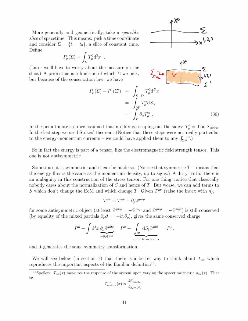
More generally and geometrically, take a spacelikeslice of spacetime. This means: pick a time coordinateand consider Σ = t = t0, a slice of constant time.Define

Pµ(Σ) =

∫Σ

T 0µd3x .

(Later we’ll have to worry about the measure on theslice.) A priori this is a function of which Σ we pick,but because of the conservation law, we have

Pµ(Σ)− Pµ(Σ′) =

∫Σ−Σ′

T 0µdDx

=

∫∂V

Tαµ dSα

=

∫V

∂αTαµ . (36)

In the penultimate step we assumed that no flux is escaping out the sides: T iµ = 0 on Σsides.In the last step we used Stokes’ theorem. (Notice that these steps were not really particularto the energy-momentum currents – we could have applied them to any

∫Σj0.)

So in fact the energy is part of a tensor, like the electromagnetic field strength tensor. Thisone is not antisymmetric.

Sometimes it is symmetric, and it can be made so. (Notice that symmetric T µν means thatthe energy flux is the same as the momentum density, up to signs.) A dirty truth: there isan ambiguity in this construction of the stress tensor. For one thing, notice that classicallynobody cares about the normalization of S and hence of T . But worse, we can add terms toS which don’t change the EoM and which change T . Given T µν (raise the index with η),

T µν ≡ T µν + ∂ρΨµνρ

for some antisymmetric object (at least Ψµνρ = −Ψρνµ and Ψµνρ = −Ψµρν) is still conserved(by equality of the mixed partials ∂ρ∂ν = +∂ν∂ρ), gives the same conserved charge

P µ +

∫d3x ∂ρΨ

µ0ρ︸ ︷︷ ︸=∂iΨµ0i

= P µ +

∫∂Σ

dSiΨµ0i︸ ︷︷ ︸

=0 if Ψ→ 0 at ∞

= P µ.

and it generates the same symmetry transformation.

We will see below (in section 7) that there is a better way to think about Tµν whichreproduces the important aspects of the familiar definition15.

15Spoilers: Tµν(x) measures the response of the system upon varying the spacetime metric gµν(x). Thatis:

Tµνmatter(x) ∝ δSmatter

δgµν(x).

41

4.1 Maxwell stress tensor

For now we can use the ambiguity we just encountered to our advantage to make an EMstress tensor which is gauge invariant and symmetric. Without the coupling to chargedparticles, we have LEM = −1

4FµνF

µν , so

T µν = − ∂L∂ (∂µAρ)

∂νAρ + δµνL

= +F µρ∂νAρ −1

4δµνFρσF

ρσ. (37)

Notice that this is not gauge invariant:

Aµ Aµ + ∂µλ =⇒ T µν T µν + F µρ∂ν∂ρλ.

We can fix this problem by adding another term

∂ρΨµνρAS = −F µρ∂ρA

ν

(this relation requires the EoM) to create a better T :

T µν = F µρF νρ −

1

4ηµνF 2.

This is clearly gauge invariant since it’s made only from F ; also it’s symmetric in µ↔ ν.

Notice also that it is traceless: ηµνTµν = T µµ = 0. This a consequence of the scale invariance

of E&M, the fact that photons are massless.

More explicitly for this case

cT 00 = 12

(~E2 + ~B2

)energy density of EM field

c2T 0i = cεijkEjBk = c(~E × ~B

)iPoynting vector (38)

The latter is both the momentum density and the energy flux, since T is symmetric. If wesubstitute in a wave solution, we’ll see that the energy in the wave is transported in thedirection of the wavenumber at the speed of light.

What’s the interpretation of T ij?

0 = ∂µTµν ν=0

=⇒ 1

c∂tT

00 + ∂iT0i = 0

The energy inside a box (a region of space) D is

Ebox =

∫D

cT 00d3x.

42

d

dtEbox =

∫D

cT 00d3x = −∫D

c2∂iT0id3x = −c2

∫∂D

T 0idSi.

So c2T 0i is the energy flux, like we said.

0 = ∂µTµν ν=j

=⇒ 1

c∂tT

i0 + ∂jTij = 0

P i =

∫D

d3xT i0 is the momentum in the box.

dP i

dt=

∫D

d3x∂0Ti0 = −

∫D

d3xc∂jTij = −c

∫∂D

dSjTij

So cT ij measures the flow of i-momentum in the j direction. Notice that the reason thatmomentum changes is because of a force imbalance: some stress on the sides of the box – if∂D were a material box, the sides would be pushed together or apart. Hence, T ij is called thestress tensor. Altogether T µν is the stress-energy-momentum tensor, but sometimes some ofthese words get left out.

4.2 Stress tensor for particles

∂µTµνEM = 0 if F obeys the vacuum Maxwell equations.

If we couple our Maxwell field to charged matter as in §3.3 the Maxwell stress tensor is nolonger conserved, but rather

∂µTµνEM = −1

cjρF ν

ρ (39)

so that P µEM =

∫d3xT 0µ

EM no longer has P µEM = 0. The EM field can give up energy and

momentum to the particles. We can rewrite this equation (39) as

∂µ(T µνEM + T µνparticle

)= 0

that is – we can interpret the nonzero thing on the RHS of (39) as the divergence of theparticles’ stress tensor. This gives us an expression for T µνparticle!

In more detail: consider one charged particle (if many, add the stress tensors) with chargee and mass m. The current is

jµ(x) = e

∫ ∞−∞

dsδ4(x− x0(s))dxµ0ds

so

∂µTµνEM = −e

c

∫dsδ4(x− x0(s)) F ν

ρ

dxρ0ds︸ ︷︷ ︸

Lorentz Force

43

Using 0 =δSparticle

δx0=⇒ mc2 d

ds

(xµ/√−x2

)= eF µ

ρdxρ

dswe have

F νρ

dxρ

ds=mc2

e

d

ds

(xν√−x2

0

).

=⇒ ∂µTµνEM = −mc

∫ ∞−∞

dsδ4(x− x0(s))d

ds

(xν0√−x2

0

)(

Usingd

dsδ4(x− x0(s)) = −dxµ0

ds

∂

∂xµδ4(x− x0(s))

)= −mc

∫ds

dxµ0ds

∂µδ4(x− x0(s))

xν0√−x2

0

= −∂µ

(mc

∫ds

xµ0 xν0√−x2

0

δ4(x− x0(s))

)︸ ︷︷ ︸

Tµνparticle

(40)

To recap what we just did, we constructed T µνparticle

T µνparticle = mc

∞∫−∞

dsδ4(x− x0(s))xµ0 x

ν0√−x2

0

so that∂µ(T µνEM + T µνparticle

)= 0

on solutions of the EoM δStotal

δx0= 0 and δStotal

δA= 0, where Stotal is the action (32).

Notice that the dependence on the charge cancels, so we can use this expression even forneutral particles. (Later we will have a more systematic way of finding this stress tensor.)Also notice that this T µνparticle = T νµparticle is symmetric.

44

4.3 Fluid stress tensor

Now consider a collection of particles en,mn with trajectories xµn(s), n = 0, 1, ....

T µνparticles(x) =∑n

mnc

∫dsδ4(x− xn(s))

xµnxνn√−x2

n

We are going to extract from this a coarse-grained description of the stress-energy tensorof these particles, thinking of them as (an approximation to) a continuum fluid. It’s a littlebit involved.

T µνparticles =∑n

mnc

∫dsδ(x0 − x0

n(s))δ3(~x− ~xn(s))xµnx

νn√−x2

n

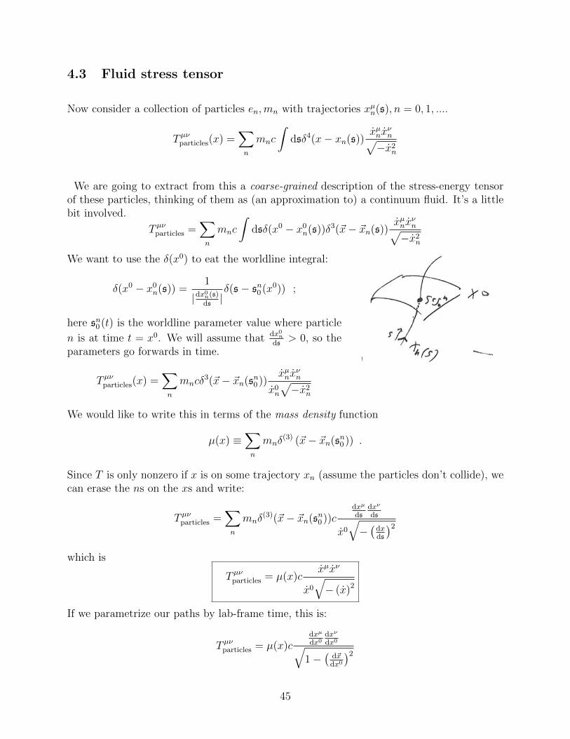
We want to use the δ(x0) to eat the worldline integral:

δ(x0 − x0n(s)) =

1

|dx0n(s)ds|δ(s− sn0 (x0)) ;

here sn0 (t) is the worldline parameter value where particle

n is at time t = x0. We will assume that dx0n

ds> 0, so the

parameters go forwards in time.

T µνparticles(x) =∑n

mncδ3(~x− ~xn(sn0 ))

xµnxνn

x0n

√−x2

n

We would like to write this in terms of the mass density function

µ(x) ≡∑n

mnδ(3) (~x− ~xn(sn0 )) .

Since T is only nonzero if x is on some trajectory xn (assume the particles don’t collide), wecan erase the ns on the xs and write:

T µνparticles =∑n

mnδ(3)(~x− ~xn(sn0 ))c

dxµ

dsdxν

ds

x0

√−(

dxds

)2

which is

T µνparticles = µ(x)cxµxν

x0

√− (x)2

If we parametrize our paths by lab-frame time, this is:

T µνparticles = µ(x)cdxµ

dx0dxν

dx0√1−

(d~xdx0

)2

45

Next goal: define the fluid 4-velocity field uµ(x) (a tricky procedure). 1) Pick a point inspacetime labelled xµ. 2) Find a particle whose worldline passes through this point, withsome arbitrary parametrization. 3) If you can’t find one, define u(x) = 0. 4) For points xon the worldline of some particle xn, define:

uµ(x) =xµn√−x2

n

, where xn ≡dxnds

(41)

– if there are enough particles, we’ll have a uµ(x) defined at enough points. This velocityfield is (a) is a 4-vector at each point and (b) is independent of the parametrization s→ s(s).

In terms of this velocity field, we have:

T µνparticles = µ(x)cuµuν

u0

Notice that µ is not a scalar field. Rather

ρ ≡ µ(x)

u0is a scalar field.

Altogether:

T µνparticles = cρ(x)uµ(x)uν(x) . (42)

Notice that we can apply the same logic to the current density 4-vector for a collection ofparticles. The analogous result is:

jµ =e

mρuµ .

(The annoying factor of em

replaces the factor of the mass in the mass density with a factorof e appropriate for the charge density. If you need to think about both T µν and jµ at thesame time it’s better to define ρ to be the number density.)

So these results go over beautifully to the continuum. If we fix a time coordinate x0 anduse it as our worldline coordinates in (41) then

u0(x) =1√

1− ~v2(x)c2

, ~u(x) =~v(x)/c√1− ~v2(x)

c2

.

If we set the EM forces to zero (say T µνEM = 0) then the particles’ stress tensor is conserved∂µT

µνparticles = 0; these equations have names:

ν = 0 : 0 = ∂t (ρc) + ~∇ · (ρ~u) energy conservation

ν = i : 0 = ∂t~u+(~u · ~∇

)~u Navier-Stokes (w/ no viscosity and no pressure)

[End of Lecture 5]

46

4.3.1 Pressure

[Weinberg §2.10 (page 47), Landau-Lifshitz+−−− vol II, §35]

Consider a little cube of our fluid of particles at the point x. The momentum flux through aface of the cube is a force acting on the cube −T ijdSj where dSj is an area element to a facewith normal in the j direction. In the rest frame of this fluid element (where its 4-velocityis uµ = (1,~0)µ), there is no special direction in space and the aforementioned force is

T ij(x)dSj = p(x)dSkδki

where p is the pressure. 16 In the rest frame of our chunk its momentum is zero, so T i0 = 0.And the energy density T 00 is just the rest mass density of the fluid (times c2): ρ = m

volc2.

So, we have names for the components of our stress tensor:

cT µν =

ρ 0 0 00 p 0 00 0 p 00 0 0 p

µν

(43)

This agrees with our previous expression (42) if we set uµ = (1,~0)µ and p = 0. What isthe pressure? It’s some coarse-grained description of short-ranged interactions between theparticles or some other mechanism by which the particles might exert a force on the wallsof their container (e.g. thermal excitations, Fermi degeneracy pressure...).

A perfect fluid more generally is one where we can find its stress tensor for any point in thefluid by simply boosting to the rest frame and using (43). So in the frame where its localvelocity vector if uµ(x), we get

cT µν = (p+ ε)uµuν + pηµν . (44)

(ε is the energy density, which reduces to ρc2 in the rest frame.) It’s Lorentz covariant andhas the right form when we set u to the rest frame. Now the conservation law gives a betterNavier-Stokes equation:

0 = ∂µTµi = (p+ ε) ∂µu

µui + ∂µpηµi

(that is, 0 = ma− F ).

For an imperfect fluid, there are additional terms on the RHS of (44) (the constitutiverelation) depending on the gradients of the velocity field. The terms with the fewest extraderivatives are of the form T µνviscosities ∼ η∂µuν .

16The fact that the pressure is the same in all directions for a chunk of fluid at rest is called Pascal’s Lawto intimidate you. It is of course not true for every chunk of stuff: for example a solid at rest still breaksrotation invariance. Let’s not worry about that; the gravitational effects of these deviations from rotationinvariance are teeny.

47

In the non-relativistic limit, the momentum density becomes T 0i = (p+ρ)ui; quite generally,(p+ ρ)/c2 plays the role of the mass density.

The right way to think about this study of fluids (hydrodynamics) is as an effective fieldtheory: It is an expansion in small derivatives (of the velocity field u). The ‘perfect fluid’assumption is merely the approximation that the leading term in that expansion (no deriva-tives of u at all) is exact. In that approximation, the expression (44) is the only covariantexpression we can write which reduces to the correct expression in the rest frame (43) (whichit must, again by the assumption of perfectness).

Notice that the trace of the fluid stress tensor is

(cTfluid)µµ = +(p+ ε) u2︸︷︷︸=−1

+4p = 3p− ε.

Going back to the description in terms of particles this is a sum of terms of the form

(cTparticle)µµ = mc2

∫dsδ4(x− x0(s))

x2

x0√−x2

s=t= −mc2

√1− ~v2/c2δ3(~x− ~x0(t)) ≤ 0

= 0 only if m = 0. So we learn the equation of state of relativistic particles is ε = 3p:

T µνradiation =ε

3c(4uµuν + ηµν) .

(In cosmology such a stress tensor is called ‘radiation dominated’.) And for massive particlesε > 3p. In the NR limit, ε ' µ0c

2 3p and

T µνmatter ' µ0cuµuν .

48

5 Differential Geometry Bootcamp

Q: OK, so: why are we talking about manifolds and all this mathy stuff?A: Because the Einstein equivalence principle says exactly :spacetime is a semi-Riemannian manifold. (Vaguely, it says “spacetime looks like Minkowskispacetime, locally”. Our job now is to make this precise.)

So bear with me.

We are going to make intrinsic constructions of manifolds. The surface of the Earth isan example of the kind of space we want to think about. It is clearly embedded in a thirddimension, and we can use this extra (extrinsic) structure to describe it. But in the case ofspacetime itself we don’t have the luxury of some embedding space (as far as we know) andso we must learn to do without it.

5.1 How to defend yourself from mathematicians

Here is some self-defense training. There are going to be a lot of definitions. But it will helpto provide some context – to situate our discussion within the world of mathematics. Andsome of them are actually useful.

A pertinent fact about math that I took a long time to learn and keep forgetting:

Principle of mathematical sophistication: the more horrible-sounding adjectives thereare in front of the name of a mathematical object, the simpler it is.

Here, as in math in general, we will start with something that sounds simple but is actuallytotally horrible. Then we’ll add assumptions that seem like they complicate the story, butactually make things much easier, because they rule out the pathological cases that we don’tcare about. And best of all, these assumptions come from physics.

Each of the entries in the following list is called a category. In moving from one entry tothe next in the list, we assume all of the previous properties and more – that is, we arespecifying, and ruling out pathological behaviors.

1. Topological spaces. (Can’t do anything.) it’s just a list (a collection of points) withsome notion of ‘open set’. Horrible things can happen here. The German word for ‘nothorrible’ is Hausdorff.

2. Topological manifolds. (Can do topology.) locally looks like IRn. patches glued to-gether with continuous functions. Continuous means that they map open sets to open

49

sets. But they don’t have to be differentiable!

3. Differentiable manifolds, aka smooth spaces. (Can do calculus.) Now we glue patchestogether with differentiable functions, aka diffeomorphisms.

4. Riemannian manifolds. (Can measure lengths.) All of the above and here’s a metric.

5. Semi-Riemannian manifolds. (Can measure lengths, but they might be negative.)(More precisely, the metric has signature (−+ ++), with one timelike coordinate.)

[Wald, Chapter 1, Appendix A] Let’s go through that list again in a little bit more detail:A topological space X is a set with a topology D, a family of open sets Uα ⊂ Xα∈A whichsatisfies

1. D 3 X, ∅ (The whole space X is open and so is the empty set.)

2. The intersection of a finite number of open sets is also an open set, i.e. if D 3 U1,U2,then D 3 U1 ∩ U2.

3. An arbitrary union of open sets is an open set, i.e. if ∀aUa ∈ D, then ∪aUa ∈ D (maybean infinite number of them).

Def: given x ∈ X, U ∈ D is a neighborhood of x if x ∈ U .

Here’s a decent example: X = IR with D = (a, b), a < b ∈ IR, a collection of openintervals.

Here’s a pathological example: take any X and let D = X, ∅.

Hausdorff criterion: ∀x, y ∈ X, x 6= y, ∃U ∈ D such that (s.t.) x ∈ Uand ∃V ∈ D, s.t. y ∈ Vand U ∩V = ∅. This is a necessary condition for the topology to be useful – you can separatepoints – and it excludes the second example above.(Exercise: is the Hausdorff condition equivalent to ∃U 3 x s.t. y is not in U? )

Q: when should we consider two topological spaces to be the same?A: Two topological spaces X, X are equivalent if ∃f : X → X which maps open sets to opensets. More precisely:Def: A homeomorphism (isomorphism in the category of topological spaces) (X,D) ' (X, D)is a map f : X → X which is:one-to-one (x 6= y =⇒ f(x) 6= f(y))and onto (∀x ∈ X,∃x s.t. f(x) = x, i.e. f(X) = f(X))and is bicontinuous (i.e. satisfies ∀U ∈ D, f(U) ∈ D and ∀V ∈ D,∃Us.t. V = f(U)) .

This latter condition (∀V ∈ D,∃Us.t.V = f(U)) says f is continuous.

50

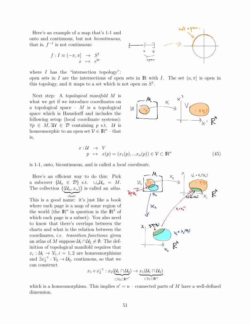
Here’s an example of a map that’s 1-1 andonto and continuous, but not bicontinuous,that is, f−1 is not continuous:

f : I ≡ (−π, π] → S1

x 7→ eix

where I has the “intersection topology”:open sets in I are the intersections of open sets in IR with I. The set (a, π] is open inthis topology, and it maps to a set which is not open on S1.

Next step: A topological manifold M iswhat we get if we introduce coordinates ona topological space – M is a topologicalspace which is Hausdorff and includes thefollowing setup (local coordinate systems):∀p ∈ M,∃U ∈ D containing p s.t. U ishomeomorphic to an open set V ∈ IRn – thatis,

x : U → Vp 7→ x(p) = (x1(p), ...xn(p)) ∈ V ⊂ IRn (45)

is 1-1, onto, bicontinuous, and is called a local coordinate.

Here’s an efficient way to do this: Picka subcover Uα ∈ D s.t. ∪αUα = M .The collection (Uα, xα)︸ ︷︷ ︸

chart

is called an atlas.

This is a good name: it’s just like a bookwhere each page is a map of some region ofthe world (the IRn in question is the IR2 ofwhich each page is a subset). You also needto know that there’s overlaps between thecharts and what is the relation between thecoordinates, i.e. transition functions: givenan atlas of M suppose U1∩U2 6= ∅: The def-inition of topological manifold requires thatxi : Ui → Vi, i = 1, 2 are homeomorphismsand ∃x−1

2 : V2 → U2, continuous, so that wecan construct

x1 x−12 : x2(U1 ∩ U2︸ ︷︷ ︸

⊂V2⊂IRn′

)→ x1(U1 ∩ U2)︸ ︷︷ ︸⊂V1⊂IRn

which is a homeomorphism. This implies n′ = n – connected parts of M have a well-defineddimension.

51

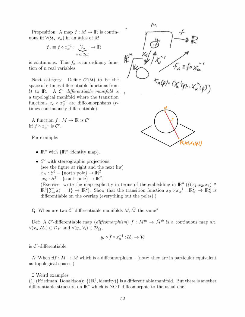
Proposition: A map f : M → IR is contin-uous iff ∀(Uα, xα) in an atlas of M

fα ≡ f x−1α : Vα︸︷︷︸

≡xα(Uα)

→ IR

is continuous. This fα is an ordinary func-tion of n real variables.

Next category. Define Cr(U) to be thespace of r-times differentiable functions fromU to IR. A Cr differentiable manifold isa topological manifold where the transitionfunctions xα x−1

β are diffeomorphisms (r-times continuously differentiable).

A function f : M → IR is Criff f x−1

α is Cr.

For example:

• IRn with IRn, identity map.

• S2 with stereographic projections(see the figure at right and the next hw)xN : S2 − north pole → IR2

xS : S2 − south pole → IR2.(Exercise: write the map explicitly in terms of the embedding in IR3 ((x1, x2, x3) ∈IR3|

∑i x

2i = 1 → IR2). Show that the transition function xS x−1

N : IR2N → IR2

S isdifferentiable on the overlap (everything but the poles).)

Q: When are two Cr differentiable manifolds M, M the same?

Def: A Cr-differentiable map (diffeomorphism) f : Mm → M m is a continuous map s.t.∀(xα,Uα) ∈ DM and ∀(yi,Vi) ∈ DM ,

yi f x−1α : Uα → Vi

is Cr-differentiable.

A: When ∃f : M → M which is a diffeomorphism – (note: they are in particular equivalentas topological spaces.)

∃ Weird examples:(1) (Friedman, Donaldson): (IR4, identity) is a differentiable manifold. But there is anotherdifferentiable structure on IR4 which is NOT diffeomorphic to the usual one.

52

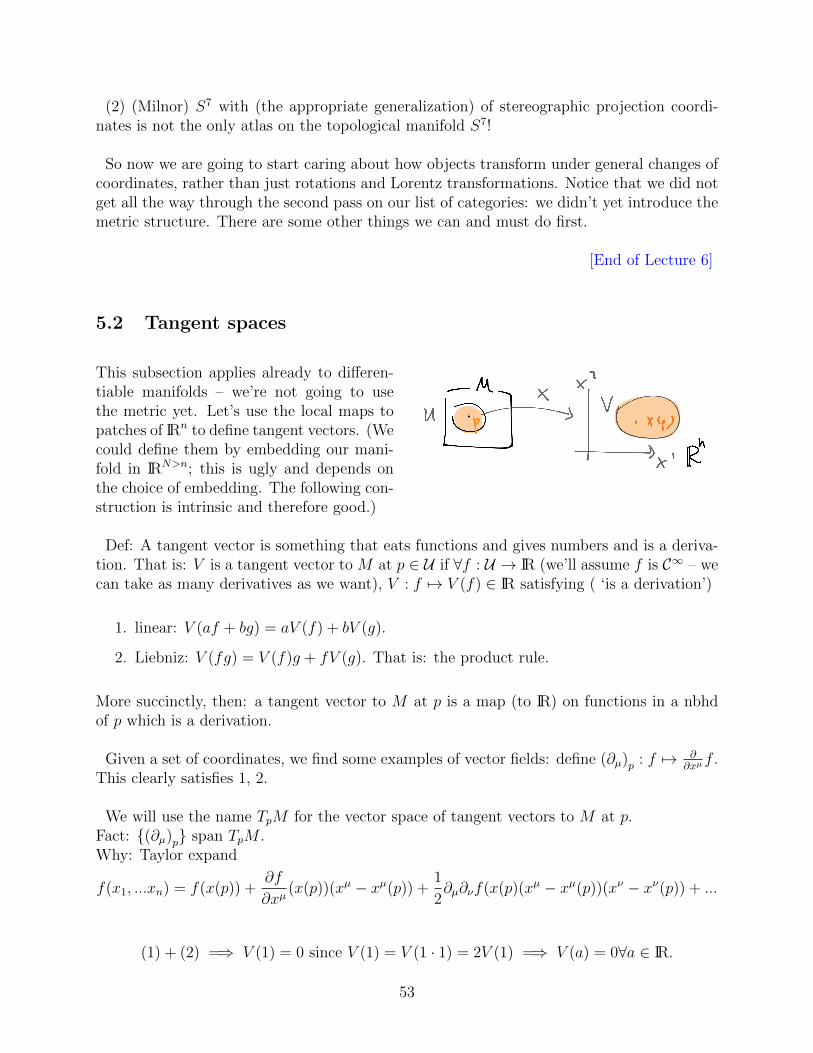
(2) (Milnor) S7 with (the appropriate generalization) of stereographic projection coordi-nates is not the only atlas on the topological manifold S7!

So now we are going to start caring about how objects transform under general changes ofcoordinates, rather than just rotations and Lorentz transformations. Notice that we did notget all the way through the second pass on our list of categories: we didn’t yet introduce themetric structure. There are some other things we can and must do first.

[End of Lecture 6]

5.2 Tangent spaces

This subsection applies already to differen-tiable manifolds – we’re not going to usethe metric yet. Let’s use the local maps topatches of IRn to define tangent vectors. (Wecould define them by embedding our mani-fold in IRN>n; this is ugly and depends onthe choice of embedding. The following con-struction is intrinsic and therefore good.)

Def: A tangent vector is something that eats functions and gives numbers and is a deriva-tion. That is: V is a tangent vector to M at p ∈ U if ∀f : U → IR (we’ll assume f is C∞ – wecan take as many derivatives as we want), V : f 7→ V (f) ∈ IR satisfying ( ‘is a derivation’)

1. linear: V (af + bg) = aV (f) + bV (g).

2. Liebniz: V (fg) = V (f)g + fV (g). That is: the product rule.

More succinctly, then: a tangent vector to M at p is a map (to IR) on functions in a nbhdof p which is a derivation.

Given a set of coordinates, we find some examples of vector fields: define (∂µ)p : f 7→ ∂∂xµ

f .This clearly satisfies 1, 2.

We will use the name TpM for the vector space of tangent vectors to M at p.Fact: (∂µ)p span TpM .Why: Taylor expand

f(x1, ...xn) = f(x(p)) +∂f

∂xµ(x(p))(xµ − xµ(p)) +

1

2∂µ∂νf(x(p)(xµ − xµ(p))(xν − xν(p)) + ...

(1) + (2) =⇒ V (1) = 0 since V (1) = V (1 · 1) = 2V (1) =⇒ V (a) = 0∀a ∈ IR.

53

=⇒ V (f) = V ( f(x(p))︸ ︷︷ ︸const =⇒ 0

+V (∂f

∂xµ(x(p))(xµ − xµ(p)))︸ ︷︷ ︸

= ∂f∂xµ

(x(p))V (xµ−xµ(p))

+...

V (f) = 0 + ∂µfpV (xµ) +1

2∂µ∂νfp V ((xµ − xµ(p))(xν − xν(p)))︸ ︷︷ ︸

=V (xµ)(xν−xν(p))+(xµ−xµ(p))V (xν)|p=0

So:

V (f) =∂f

∂xµ(p)V µ .

Summary: the tangent vector space TpM is

TpM 3 V : f 7→ V (f) ∈ IR with V (f) = V µ ∂

∂xµf(p)

Perhaps you are not used to thinking of vectors as such a map – as a differential operator.This operator is just the directional derivative (in the direction of the thing you usually thinkof as the vector). It contains the same information.

How does changing coordinates act on such a vector? Simple: it doesn’t. That is, ∀f ∈C∞(U), the value of V (f) shouldn’t change!

But the components of the vector in the coordinate basis V µ certainly do change: underxµ → xµ(x),

V (f) = V µ

(∂f

∂xµ

)p

!= V µ

(∂f

∂xµ

)p

= V µ

(∂xν

∂xµ

)p

(∂f

∂xν

)p

=⇒ V µ

(∂xν

∂xµ

)p

= V ν

To go in the other direction: because(∂xν

∂xµ

)p

(∂xµ

∂xρ

)p

= δνρ

(or by using the symmetry between tilded and untilded vars) the inverse transformation is

V µ

(∂xν

∂xµ

)p

= V ν

To emphasize: as a differential operator, V is coordinate independent:

V = V µ ∂

∂xµ|p = V µ ∂

∂xµ|p .

54

Fundamental principle of relabelling: Physics shouldn’t depend on what coordinateswe use to describe it.

Or as Zee says: physics should not depend on the physicist [Zee page 334].

Compare with the previous mention that was made of vectors: tangent vector to a curve,s 7→ xµ(s) we defined to be V µ ≡ dxµ

ds. Meaning: these are the components of the tangent

vector to the curve in the coordinate basis:

V =dxµ

ds

∂

∂xµ

Notice that if we change coordinates on spacetime xµ → xµ this object manifestly stays thesame.

In fancier language: a differentiable curve in M is a map

ϕ : (a, b)︸ ︷︷ ︸⊂IR

→M

with the following properties. If we pick p ∈ U ⊂ M (U an open set with coordinate xµ) inthe image of ϕ, and let ϕµ = xµ(ϕ) – that is

ϕµ(s ∈ (a, b)) = xµ(ϕ(s)︸︷︷︸∈M

) ,

then if we are given a function f ∈ C∞(U) we can restrict f to ϕ(a, b) and construct thetangent vector

d

dsf(φ(t))|s0︸ ︷︷ ︸∈IR

chain rule=

∂f

∂xµ

(dϕµ

ds

)(t0)

so V = dφµ

ds∂∂xµ

, i .e. V µ = dφµ

ds.

Def of tangent vector field: this is just a tangent vector at every point. The name for thecollection of tangent spaces at each point is the tangent bundle TM .

V : M → TMp 7→ Vp ∈ TpM (46)

An example of a vector field on the sphere is obtained by embedding it in IR3 and rotatingit: define vp to be the velocity of the sphere at each point (it vanishes at the poles).

Def of commutator (aka Lie bracket): consider u = uµ∂µ. Define a product of vectorfields by thinking of them as differential operators and acting twice on the same function:uvf = uµ∂µ (vν∂νf).

[v, u] = vu− uv = [vµ∂µ, uν∂ν ] = vµ∂µ (uν∂ν)− uν∂ν (vµ∂µ) = (vµ (∂µu

ν)− uµ (∂µvν)) ∂ν

55

also a (contravariant) vector field. So the set of vector fields on M with [, ] form a closedalgebra. In fact it is a Lie algebra (i.e. the bracket satisfies the Jacobi identity).

A vector field on M produces a flow, that is, a one-parameter family of maps φv(s) : M →M with φ(s) φ(t) = φ(s+ t) and each φ(s) is smooth and 1-1. The map is arranged so thatthe vector field is tangent to the flow line going through each point, that is, the flow linesare integral curves of the vector field. Let xµ label a point p. Then φv(s)(p) has coordinatesxµ(s), where

d

dsxµ(s) = vµ(x) (47)

is an ordinary differential equation for xµ(s); the initial condition that φ(s = 0) = 1, theidentity map, translates to xµ(0) = xµ. Notice that flows and vector fields contain the sameinformation; if we are given φ(s), we can construct the associated v using (47) in the otherdirection.

A reason to care about the commutators of vector fields is if you want to compare theresults of their flows; flowing by commuting vector fields you end up at the same point nomatter which order you do the flows in. (A more precise statement is called the FrobeniusTheorem, which I will not discuss.)

5.2.1 Cotangent vectors

equals one-forms. This is something that eats a vector and gives a number, and is linear.That is, the space of cotangent vectors T ?pM is the dual space (in the sense of linear algebra)to TpM : the vector space of linear maps from TpM to IR.

ω : TpM → IRV 7→ ω(V ) and ω(aV + bW ) = aω(V ) + bω(W ) (∀a, b ∈ IR)

dimT ?pM = dimTpM

since an element is determined by its action on a basis of TpM .

In a basis, if V = V µ∂µ, then

ω(V ) = V µω(∂µ) ≡ V µωµ.

Linear eating is just contraction of the indices.

Example of a one-form: Given a function on M , we can make a one-form as follows. Recallthat v ∈ TpM maps f 7→ v(f)|p = vµ (∂µf)p ∈ IR (the directional derivative). f thendefines a cotangent vector by v 7→ v(f). This is a linear map: av + bw 7→ av(f) + bw(f) =(avµ + bwµ) ∂µf |p. Denote this cotangent vector df |p ∈ T ?pM .

df |p ∈ T ?pM is defined by df |p : M → IR

56

v 7→ df |p(v) ≡ v(f). (48)

Coordinates induce a basis for T ?pM , just as they do for TpM . If

x : U → IRn

p 7→ (x1(p)...xn(p)) (49)

then each xµ is a function on M in a neighborhood of p. The associated cotangent vectorsare

dxµ|p : TpM → IRv 7→ dxµ(v) ≡ v(xµ) = vν∂νx

µ = vµ (50)

(dxµ)p , µ = 1..nis a basis of T ?pM since ω = ωµdxµ|p is an arbitrary 1-form: for any v ∈ TpM ,

ω(v) = ωµdxµ|p (vν∂ν)linearity

= ωµvν dxµ|p (∂ν)︸ ︷︷ ︸

=∂νxµ=δµν

= ωµvµ

and any linear functional on TpM has this form.

And under a coordinate transformation xµ → xµ,

∂µ → ∂µ =∂xν

∂xµ∂ν =⇒ v = vµ∂µ = vµ∂µ =⇒ vµ =

∂xµ

∂xνvν

dxµ → dxµ =∂xµ

∂xνdxν =⇒ ω = ωµdxµ = ωµdxµ =⇒ ωµ =

∂xν

∂xµων (51)

contravariant: v → v with vµ(x) =∂xµ

∂xνvν(x)

covariant: ω → ω with ωµ(x) =∂xν

∂xµvν(x)

worth noticing:

dxµ(v) ≡ v(xµ) = vν∂νxµ = vµ =⇒ vν ∂ν x

µ ≡ v(xµ) = dxµ(v) = vµ.

5.2.2 Tensor fields.

A rank

(sr

)tensor is

t ∈ T ?pM ⊗ ....⊗ T ?pM︸ ︷︷ ︸r

⊗TpM ⊗ ....⊗ TpM︸ ︷︷ ︸s

57

In the coordinate bases it is

t = tν1...νsµ1..µr

(x)dxµ1 ⊗ · · · ⊗ dxµr ⊗ ∂

∂xν1⊗ · · · ⊗ ∂

∂xνs

– it is a thing which eats r vectors and s cotangent vectors at once and gives a number (andit is linear in each feed-hole). (The fancy symbol ⊗ is just meant to indicate this linearity

in each argument, and will often be omitted.) An example of a rank

(02

)tensor is a metric

– it eats two vectors at a time.

Note: so far “d” is not an operator in that we haven’t explained how it acts on anythingother than functions, i.e.

d : C∞(M) → T ?Mf 7→ df (52)

(and we also haven’t explained how to use it as something to integrate) It’s not hard todefine the exterior derivative on one-forms:

d : T ?pM →(T ?pM ⊗ T ?pM

)AS

ω = ωµdxµ 7→ (∂µων − ∂νωµ) dxµ ⊗ dxν (53)

‘AS’ stands for antisymmetric. Notice that d2 = 0 by equality of mixed partials. Notice thatthe components (dω)µν = ∂µων − ∂νωµ are antisymmetric; this allows us to write

dω ≡ (∂µων − ∂νωµ) dxµ ∧ dxν

– the wedge product means that the basis one-forms are antisymmetrized. A differentialform of rank r can then be expanded as:

ω = ωµ1···µrdxµ1 ∧ ... ∧ dxµr .

Demanding that the d2 = 0 property continue, we can define the exterior derivative onp-forms of arbitrary rank.

The Lie derivative on vector fields can be defined in a similar way, so far without metric.But curvatures and connections require a metric.

5.2.3 ENTER THE METRIC.

First, let’s consider metric on the tangent space TpM – it’s just an inner product betweentangent vectors.

g(·, ·) : TpM × TpM → IR(u, v) 7→ g(u, v) . (54)

58

It is bilinear (g(au+ bu, v) = ag(u, v) + bg(u, v),∀a, b ∈ IR. same for v → av + bv)and symmetric (g(u, v) = g(v, u))

In terms of components (by linearity), this is

g(u, v) = uµvνg((∂µ)p , (∂ν)p) ≡ uµvνgµν |p.

So symmetry says gµν |p = gνµ|p.

Notice that g|p is a thing that eats two vectors in TpM and gives a number (and is linearin each argument) – this is exactly the definition of an element of T ?pM ⊗T ?pM – a rank twocovariant tensor. We can expand such a thing in a coordinate basis for each factor:

g = gµνdxµ ⊗ dxν .

We have already seen such a thing and called it ds2, the line element, omitting the ⊗ symbol.

Now demand that g(u, v) is independent of coordinates. This tells us (I hope you aregetting used to this stratagem) how gµν transforms:

g(u, v) = uµvνgµν |p!

= uµvν gµν |p

This says that g is a rank-2 covariant tensor17:

gµν |p =

(∂xρ

∂xµ

)p

(∂xσ

∂xν

)p

gρσ(p).

Alternatively we could arrive at this conclusion using linearity:

gµν = g(∂µ|p, ∂ν |p) = g(∂xρ

∂xµ∂ρ,

∂xσ

∂xν∂σ)

linearity=

∂xρ

∂xµ∂xσ

∂xνgµν

Since gµν |p is a symmetric matrix, it has real eigenvalues. Their signs determine the signa-ture of the metric. Three plus and one minus will be the relevant case for us.

Important remarks:

1. To get a metric on TM from the ones on TpM for each point p, just erase the psubscripts.

17Notice by the way that I am abusing the terminology a bit, using the term ‘tensor’ for both the coordinate-invariant fancy thing g and for the collection of its components in a coordinate basis gµν , which actually dochange under coordinate transformations. If you find this confusing then I suggest the following exercise:make up different names for the two things and go through the lecture notes and correct every appearanceof the word tensor. If after doing that you think it’s worth making this distinction, come try to convince me.

59

2. In general, the components of the metric depend on coordinates (in a smooth way, wewill assume).

3. Notice that we haven’t discussed where to find gµν(x); until our discussion of Einstein’sequations, we will just assume that we’ve found one in our basement or something.

4. Any expression made of tensors with all indices contracted is invariant under generalcoordinate transformations. This is the point of going through all this trouble.

Proof: use explicit expressions for transformation laws.

Why gµν – the metric on spacetime – is symmetric: the EEP. At any point in spacetime x,you have to be able to choose coordinates so that locally it looks like Minkowski spacetime,i.e. gµν(x) = ηµν , which is symmetric. Under a coordinate change to any general coordinatesystem,

gµν 7→ gµν =∂xρ

∂xµ∂xσ

∂xνgρσ

which is still symmetric. [End of Lecture 7]

Here is a list of uses of the metric: basically we can put it everywhere we had an ηµνwhen we were working in Minkowski space. There are a few places where the η was hidden,e.g. because | det η| = 1.

1. lengths of vectors: ||v ||2 = gµνvµvν . The sign of this quantity still distinguishes timelike

from spacelike vectors.

2. angles between vectors at the same point: gµνV µW ν

|| V ||||W || .

3. lengths of curves: add up the lengths of the tangent vectors L[x] =∫

ds√|gµν dxµ

dsdxν

ds|.

Hence, we can make actions for particles in curved spacetime.

4. inverse metric: if the metric at p is non-degenerate (detµν gµν 6= 0) then its inverse asa matrix exists:

gµν(g−1)νρ

= δρµ

it is convenient to write this statement as

gµνgνρ = δρµ

– that is, we denote the matrix inverse with upper indices and don’t need to writethe inverse symbol. Notice that this worked for free with ηµν and δij since as matricesthey were their own inverse. Notice that the inverse metric is a tensor field with twocontravariant indices.

5. A non-degenerate metric allows us to identify TpM and T ?pM

v = vµ∂µ 7→ v? ≡ gµνvνdxµ

60

The map from TpM to T ?pM is

v 7→(v? : TpM → IR

u 7→ v?(v) ≡ g(v, u)

)So v?(·) = g(v, ·). This is what we mean by lowering indices. That is, we don’t needto write the stars if we write the indices: given a vector vµ, we can define v?µ ≡ vµ.Similarly, raising indices is just a convenient notation for the map g−1 : T ?pM → TpM .And this dropping-stars notation justifies our notation (g−1)

µν ≡ gµν because

gµν = (g??)µν =(g−1)µρ (

g−1)νσ

gρσ =(g−1)µρ

δνσ =(g−1)µν

.

6. Volumes.

(Preview: we’re going to use this to define actions and covariant derivatives.)

We’re going to want to write S =∫M

dDxL(x) where L(x) is some (scalar) function onx.

[Here L will depend on x via various fields, and the point of S is so we can vary it;δSδφ(x)

= 0 is the EOM.]

But dDx is not coordinate invariant.

Claim: dDx√g is coordinate invariant. Here, by

√g I mean

√| det g|. I am omitting

the abs by convention. If you like I am defining g ≡ − det g. det g = detµν gµν .

Proof:

xµ = xµ(xν). Jµν ≡∂xµ

∂xν

gµν =(J−1)αµ

(J−1)βνgαβ.

det g = det J−2 det g, dDx = det JdDx.

So: √gdDx =

√gdDx.

7. Make a stress tensor. Put some stuff (a classical field theory) on a spacetime with ametric. By varying the metric at a point, we can probe the response of the stuff. We’lldo this in §7.

8. Derivatives of tensors which are tensors (next).

61

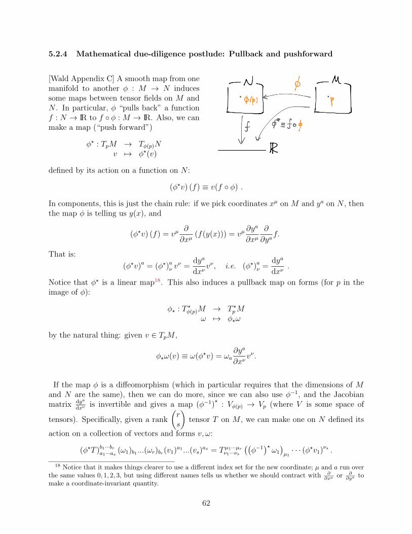
5.2.4 Mathematical due-diligence postlude: Pullback and pushforward

[Wald Appendix C] A smooth map from onemanifold to another φ : M → N inducessome maps between tensor fields on M andN . In particular, φ “pulls back” a functionf : N → IR to f φ : M → IR. Also, we canmake a map (“push forward”)

φ? : TpM → Tφ(p)Nv 7→ φ?(v)

defined by its action on a function on N :

(φ?v) (f) ≡ v(f φ) .

In components, this is just the chain rule: if we pick coordinates xµ on M and ya on N , thenthe map φ is telling us y(x), and

(φ?v) (f) = vµ∂

∂xµ(f(y(x))) = vµ

∂ya

∂xµ∂

∂yaf.

That is:

(φ?v)a = (φ?)aν vν =

dya

dxνvν , i.e. (φ?)aν =

dya

dxν.

Notice that φ? is a linear map18. This also induces a pullback map on forms (for p in theimage of φ):

φ? : T ?φ(p)M → T ?pMω 7→ φ?ω

by the natural thing: given v ∈ TpM ,

φ?ω(v) ≡ ω(φ?v) = ωa∂ya

∂xνvν .

If the map φ is a diffeomorphism (which in particular requires that the dimensions of Mand N are the same), then we can do more, since we can also use φ−1, and the Jacobianmatrix dya

dxνis invertible and gives a map (φ−1)

?: Vφ(p) → Vp (where V is some space of

tensors). Specifically, given a rank

(rs

)tensor T on M , we can make one on N defined its

action on a collection of vectors and forms v, ω:

(φ?T )b1···bra1···as (ω1)b1 ...(ωr)br(v1)a1 ...(vs)as = T µ1···µr

ν1···νs

((φ−1)?ω1

)µ1· · · (φ?v1)νs .

18 Notice that it makes things clearer to use a different index set for the new coordinate; µ and a run overthe same values 0, 1, 2, 3, but using different names tells us whether we should contract with ∂

∂xµ or ∂∂ya to

make a coordinate-invariant quantity.

62

The way to read this equation is: “stick the matrix dya

dxνor its inverse dxµ

dyawherever you need

to in order to get the indices to work out”. I will not keep careful track of where the starsand inverses are. In any example, there’s only one right place to put them, so there’s noneed for them.

Recall that diffeomorphic was the precise notion of same in the category of smooth mani-folds. The existence of a diffeomorphism φ : M → N means that the two manifolds are justrelated by a change of coordinates. Classical field theories on these two manifolds thereforeproduce the same physics. The previous discussion shows how to use this to translate all thetensor fields living on M into tensor fields living on N .

5.2.5 Appendix: Integration of forms over submanifolds

We can describe a submanifold Σ of a manifold M in two very different ways: by givingconditions on coordinates of M which specify where Σ is (such a thing is called a varietyfor some reason), or by embedding Σ into M by maps from some auxiliary parameter space.We’ll discuss these in order, and how to think about integrals in each case.

1. So for example we can specify Σn−k ⊂Mn by giving k (independent, local) conditions

Σ = yα = 0, α = 1...k

the number of such conditions is called the codimension of Σ. (In general, these con-ditions may have to be locally specified in order to be independent. This is a longstory.)

Then, given a n − k form on M , we can define a number by integrating it over thesubmanifold Σn−k by∫

Σn−k

ωn−k =

∫M

ωn−k ∧ dy1 ∧ ... ∧ dykδk(y)

On the RHS is an integral of an n-form over all of M , which (if M is connected) itmust be proportional to the volume form. Notice that this is a direct generalization ofour expression for

∫worldline

A the minimal coupling term in the worldine action in (28).

2. Alternatively, suppose we are given some maps whose image is Σ:

x : U ⊂ IRn−k → M(σα)α=1..n−k 7→ (xa(σ))a=1..n

This generalizes our notion of a parametrized curve xµ(s). Notice that we haven’t saidanything about the parametrization. Again these maps may need to be defined locally.

63

In this case we can define the integral of a form of appropriate rank by∫Σn−k

ωn−k =

∫dσ1 · · · dσn−kεα1...αn−k

∂xa1

∂σα1· · · ∂x

an−k

∂σαn−kωa1...an−k .

(If I wanted to be pedantic I would write this as∫Σn−k

x?ωn−k

where x? is the pullback of the form by the map x to a form U .)

Notice that Stokes’ theorem is beautifully simple in this notation:∫∂Σ

ω =

∫Σ

dω

where ∂Σ is the boundary of Σ (and gives zero if Σ has no boundary).

Notice that we didn’t use the metric in the above discussion. This implies another possibil-ity for covariantly integrating things to make actions, besides the

∫ √g(scalar) strategy that

we used above. If, amongst our fields for which we’re constructing an action, are some dif-ferential forms, and we can wedge19 them together to make a form Ω = Ωa1···andx1∧· · ·∧dxn

of rank n = dimM , we can integrate∫M

Ω =

∫dnxΩ1···n

and it is coordinate invariant. This is because under a coordinate transformation dnx =det Jdnx, while Ω1···n = det−1 JΩ1···n.

A simple example is in Maxwell theory in four dimensions. In that case F = dA is atwo-form, and we can make a four-form which is gauge invariant by F ∧ F . The resultingterm

θ

16π2

∫M

F ∧ F

is generally covariant, independent of the metric. It is the same as ?F µνFµν ∝ ~E · ~B. Such aterm which is generally covariant, independent of the metric is said to be topological. Anotherimportant example arises in gauge theory in 2 + 1 dimensions, where SCS[A] ≡ k

4π

∫A ∧ F

is called a Chern-Simons term.

19 By ‘wedge’ I mean the following. We showed earlier how to make a p+ 1 form from a p form by exteriorderivative. Given a p-form ω = ωa1···apdxa1 ∧ ...∧dxap and a q-form µ = µb1···bqdx

b1 ∧ ...∧dxbq we can makea p+ q-form by antisymmetrizing the product:

ω ∧ µ ≡ ωa1···apµb1···bqdxa1 ∧ ... ∧ dxap ∧ dxb1 ∧ ... ∧ dxbq .

64

5.3 Derivatives

Consider V µ(x), the components of a vector field in a coordinate basis. We want to differ-entiate the vector field.

What not to do: What might we mean by ∂νVµ? Under a change of coordinates xµ → xµ,

∂νVµ 7→ ∂xα

∂xν∂α

(∂xµ

∂xβV β

)= ∂νx

α∂βxµ∂αV

β +(∂νx

α∂β∂αxµ)V β. (55)

This is not a tensor! Also from (55) you see why antisymmetrizing is a good idea, and theexterior derivative is perfectly coordinate invariant.

How to take a derivative of a tensor and get a tensor?

For scalar quantities there’s no problem. Consider a scalar field living on some R’n manifold,φ(x). Like temperature of CMB. Or the Higgs condensate. ∂µφ is perfectly coordinatecovariant. It transforms like a vector.

Q: Is there an intrinsic definition of derivatives?

A: At least two.

5.3.1 Lie Derivative

Given a vector field v on M , we know how to use it to take a derivative of a function f onM in a coordinate-invariant way:

vf = vµ∂µf ≡ Lvf

– this (directional derivative) is sometimes called the Lie derivative of f along v.

The general def of a Lie derivative of a tensor T along a vector field v is as follows. Recallthat vector field on M produces a flow φs : M → M (the v will be implicit here). The Liederivative of T along v is:

LvT (p) = lims→0

(φ?−sT (φs(p))− T (p)

s

)Notice that the difference on the RHS is between tensors at the same point p, since φ?−s :Vφs(p) → Vp.

For a function, this is just

Lvf(p) =d

ds(f(φs(p))) |s=0

def of φ=

dxµ

ds

∂f

∂xµ= vµ

∂f

∂xµ= vf.

65

The Lie derivative of a vector field w along a vector field v is

Lvw ≡ [v, w]

– it’s just the commutator. This is a useful exercise in unpacking the definition of thepullback map. 20

Given a vector field v, we can also construct explicitly the Lie derivative along v of othertensor fields. To figure out the explicit form, note again from the definition that Lv is Liebniz,so

Lv(ω(Y ))︸ ︷︷ ︸known

= (Lvω)Y + ω LvY︸︷︷︸known

.

One point of Lie derivative is to detect symmetries of the metric. The statement that forsome vector field v

Lvg = 0

means that the metric doesn’t change along the flow by v – it’s a symmetry of g. Such a vis called a Killing vector field.

Summary of properties:

on a function, it gives: Lvf = vf

on a vector field, it gives: Lvw = [v, w]

it’s linear: Lv (aT1 + bT2) = aLvT1 + bLvT2

it’s Liebniz: Lv (T1T2) = (LvT1)T2 + T1 (LvT2) .

Recall that the last two combine to the statement that Lv is a derivation.

20Here we go. Expanding in a coordinate basis for TpM v = vµ∂µ, w = wµ∂µ, we have

Lvw = Lv(wµ

∂

∂xµ

)= vν∂νw

µ ∂

∂xµ+ wµLv

(∂

∂xµ

)using the Liebniz property. Now

Lv(

∂

∂xµ

)≡ limt→0

φv(−t)?(∂∂xµ

)− ∂

∂xµ

t= − ∂v

ν

∂xµ∂

∂xν.

Putting these together gives the coordinate expression for the commutator:

Lvw = (wµ∂µvν − vµ∂µwν)

∂

∂xν= [v, w].

You may like Wald’s argument for this; he choose coordinates where the flow parameter t is one of thecoords, x1 = t.

66

5.3.2 Covariant Divergence

[Zee page 326] First we are going to guess a (useful) formula for a covariant divergence thatdoes not involve the horrible Christoffel symbols. We can check that it is indeed covariant.Then we will come back and develop the fancy-pants understanding of why this is a goodconstruction (in terms of parallel transport), and how to extend it to a more general derivativeoperator.

The basic reason we want to differentiate tensors is so that we can write field equations.Where do field equations come from? (For non-dissipative systems) they come from actionprinciples. Actions are simpler – for each field configuration they give a number, usually(always in this class) a real number. Why in the world would we start by writing fieldequations, which is some horrible tensor-field-valued functional? Further, the action has tobe invariant under coordinate changes in order for physics not to depend on our choice ofcoordinates. Whereas the horrible tensor-valued functional merely has to be covariant.

This apparent detour will be useful because we’ll use the same kind of logic in constructingthe Einstein-Hilbert action for the metric.

So let’s try to guess what a coordinate invariant action functional for a scalar field in curvedspace might be. We want it to be local in spacetime, so that we don’t get action at a distance.What I mean is that it should be a single integral over spacetime

S[φ] =

∫M

L(φ, ∂µφ)

of a lagrangian density with finitely many derivatives of φ. Wait – we’re trying to figureout how to take derivatives here. But we already know how to take one derivative of φ in acovariant way, it’s just ∂µφ. So let’s just look for a lagrangian density which depends onlyon φ, ∂µφ.

So there are two things I should clarify: what I mean by∫M

, and what should we use forL? We already found a covariant integration measure above21. So more explicitly we have:

S[φ] =

∫M

dDx√gL(φ(x), ∂µφ(x))

To make scalars, contract indices.

Just for simplicity, let’s suppose φ→ φ+ ε is a symmetry (like a goldstone boson), so theaction can’t depend explicitly on φ. Then the invariant thing with the fewest derivatives is:

S[φ] =

∫M

dDx√g∂µφ∂νφg

µν

21There may be other ways to make a covariant integral; for another example, see §5.2.5.

67

[End of Lecture 8]

What are the equations of motion? If we were in flat space, it would be 2φ = 0, the waveequation. What is 2φ? In flat space it is ∂µ∂

µφ, a second derivative of φ! In curved spaceit is:

− 1√g

δS

δφ(x)=

1√g∂µ√ggµν∂νφ ≡ 2φ. (56)

(The factor of 1√g

on the LHS is to make it a scalar, rather than a scalar density.)

On HW: Similarly for Maxwell: where you see η put g, and stick a√g in the measure.

So we’ve learned to differentiate the particular vector field ∂µφ = ∇µφ = gµν∇µφ in acovariant way, but only in a certain combination. Demanding that

2φ != ∇µ∇µφ

and comparing with our expression (56) suggests that we should define

∇νVµ ?

=1√g

(∂ν√gV µ) (57)

Is this covariant? In fact, no.

68

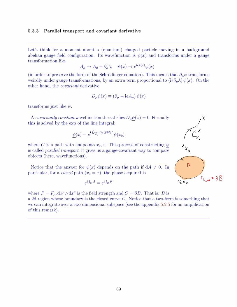
5.3.3 Parallel transport and covariant derivative

Let’s think for a moment about a (quantum) charged particle moving in a backgroundabelian gauge field configuration. Its wavefunction is ψ(x) and transforms under a gaugetransformation like

Aµ → Aµ + ∂µλ, ψ(x)→ eieλ(x)ψ(x)

(in order to preserve the form of the Schrodinger equation). This means that ∂µψ transformsweirdly under gauge transformations, by an extra term proportional to (ie∂µλ)ψ(x). On theother hand, the covariant derivative

Dµψ(x) ≡ (∂µ − ieAµ)ψ(x)

transforms just like ψ.

A covariantly constant wavefunction the satisfiesDµψ(x) = 0. Formallythis is solved by the exp of the line integral:

ψ(x) = ei∫Cxx0

Aµ(y)dyµ

ψ(x0)

where C is a path with endpoints x0, x. This process of constructing ψis called parallel transport; it gives us a gauge-covariant way to compareobjects (here, wavefunctions).

Notice that the answer for ψ(x) depends on the path if dA 6= 0. Inparticular, for a closed path (x0 = x), the phase acquired is

ei∮C A = ei

∫B F

where F = Fµνdxµ∧dxν is the field strength and C = ∂B. That is: B is

a 2d region whose boundary is the closed curve C. Notice that a two-form is something thatwe can integrate over a two-dimensional subspace (see the appendix 5.2.5 for an amplificationof this remark).

69

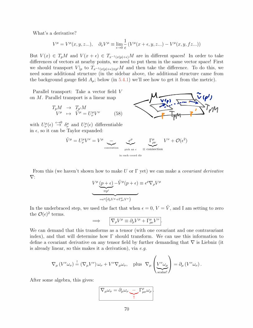
What’s a derivative?

V µ = V µ(x, y, z...), ∂xVµ ≡ lim

ε→0

1

ε(V µ(x+ ε, y, z...)− V µ(x, y, fz...))

But V (x) ∈ TpM and V (x + ε) ∈ Tx−1(x(p)+ε)M are in different spaces! In order to takedifferences of vectors at nearby points, we need to put them in the same vector space! Firstwe should transport V |p to Tx−1(x(p)+ε)≡p′M and then take the difference. To do this, weneed some additional structure (in the sidebar above, the additional structure came fromthe background gauge field Aµ; below (in 5.4.1) we’ll see how to get it from the metric).

Parallel transport: Take a vector field Von M . Parallel transport is a linear map

TpM → Tp′MV µ 7→ V µ = Uµ

ν Vν (58)

with Uµν (ε)

ε→0→ δµν and Uµν (ε) differentiable

in ε, so it can be Taylor expanded:

V µ = Uµν V

ν = V µ −︸︷︷︸convention

ερ︸︷︷︸pick an ε

in each coord dir

Γµρν︸︷︷︸≡ connection

V ν +O(ε2)

From this (we haven’t shown how to make U or Γ yet) we can make a covariant derivative∇:

V µ (p+ ε)︸ ︷︷ ︸≡p′

−V µ(p+ ε)

︸ ︷︷ ︸=ερ(∂ρV µ+ΓµρνV ν)

≡ ερ∇ρVµ

In the underbraced step, we used the fact that when ε = 0, V = V , and I am setting to zerothe O(ε)2 terms.

=⇒ ∇ρVµ ≡ ∂ρV

µ + ΓµρνVν .

We can demand that this transforms as a tensor (with one covariant and one contravariantindex), and that will determine how Γ should transform. We can use this information todefine a covariant derivative on any tensor field by further demanding that ∇ is Liebniz (itis already linear, so this makes it a derivation), via e.g.

∇µ (V νων)!

= (∇µVν)ων + V ν∇µων , plus ∇µ

V νωµ︸ ︷︷ ︸scalar!

= ∂µ (V νων) .

After some algebra, this gives:

∇µων = ∂µων −︸︷︷︸↑

Γρµνωρ .

70

Notice the change of sign in the connection term between contravariant and covariant tensors.Similarly, we can figure out how to get ∇µT

ρσ by using the Liebniz property on ∇µ (vρuσ) =... and the demand that any such tensor field gets transported the same way. This gives

∇µTρσ = ∂µT

ρσ + ΓρµλTλσ + ΓσµλT

ρλ .

I hope you see the pattern.

Now let’s talk about how Γ transforms under coordinate changes22. The demand we arereally making is that parallel transport is independent of coordinate choice. This is the same

as demanding that ∇µvν are the components of a

(11

)tensor. It transforms as

∇µvν = ∂µv

ν + Γνµρvρ 7→

∂µxρ∂σ∂ρx

νvσ+ ∂µx

ρ∂σxν

(∂ρv

σ

+Γσρκvκ

)!

= ∂µxρ∂σx

ν

(∂ρv

σ

+Γσρκvκ

)(59)

from which we infer (notice that the top lines are already equal):

Γµνρ = ∂νxσ∂κx

µ∂ρxδΓκσδ︸ ︷︷ ︸

tensor transf

− ∂κ∂δxµ∂νxκ∂ρxδ︸ ︷︷ ︸extra badness

. (60)

The extra badness in the transformation of Γ is precisely designed to cancel the badnessfrom the transformation of the ordinary derivative of the vector (55). [For more discussionof this sea of indices, see Zee page 329]

Q: What does it mean for a vector field to be constant? Consider the vector field W = ∂x inthe plane. Write its components in polar coordinates and compute their partial derivatives.[see Zee page 323 and problem set 5.]

5.4 Curvature and torsion

Given a connection Γ, there are two tensor fields you can make right away.

1) Torsion tensor ≡ the antisymmetric part of the connection.

Γµ[ρ,σ] ≡ Γµρσ − Γµσρ.

Notice that the bad stuff of the transformation law (60) (the inhomogeneous term) cancelsout of this combination:

Γµ[σ,ρ] = ∂ρxα∂σx

β∂γxµΓγ[α,β].

Below, we’ll choose a connection with no torsion, Γγ[α,β] = 0. Comments:

22Please studiously ignore Wald’s discussion of this point which could not be made more confusing.

71

1. Because the torsion is a tensor, this choice is coordinate-independent.

2. If you want you can undo this assumption. Then you will get a more complicatedtheory of gravity which is experimentally different from GR and wrong 23.

3. Some effects of this assumption:– In the exterior derivative, we can use ordinary derivative or covariant derivative andit doesn’t matter:

dω = ∇[µων]dxµ ∧ dxν =

(∂[µων] − Γρ[µ,ν]

)dxµ ∧ dxν .

In general they are both tensors, but in the torsion-free case, they are equal.

– For scalars:

∇[µ∇ν]f = ∇µ (∂νf)−∇ν (∂µf) =(∂µ∂ν − Γρµν

)f −

(∂ν∂µ − Γρνµ

)f = Γρ[ν,µ]∂ρf

so if T ρνµ ≡ Γρ[ν,µ] = 0 then ∇[µ∇ν]f – the mixed covariant derivatives commute onscalars. I emphasize those last two words because of the next item.

2) Curvature tensor.

Consider more generally what happens if we take the commutator of covariant deriva-tives, for example, when acting on a one-form. By construction, what we get is also (thecomponents of) a tensor:

∇[µ∇ν]ωρ = ∇µ∇νωρ − (µ↔ ν)= ∇µ

(∂νωρ − Γκνρωκ

)− (µ↔ ν)

=(∂µ∂νωρ − Γγµν∂γωρ − Γγµρ∂νωγ − Γκνρ∂µωκ + (terms without derivatives of ω)µν

)−

(∂ν∂µωρ − Γγνµ∂γωρ − Γγνρ∂µωγ − Γκµρ∂νωκ + (terms without derivatives of ω)νµ

)(If T = 0, derivatives of ω cancel! )

≡ Rµνρσωσ (61)

(Beware that there is some disagreement about the sign in the definition of the curvature.In particular, Zee (page 341) uses the opposite sign.)

Alternative to explicit computation above: Consider any scalar function f . Then

∇[µ∇ν] (fωρ) =(∇[µ∇ν]f

)︸ ︷︷ ︸=0 if no torsion

ωρ + f∇[µ∇ν]ωρ = f∇[µ∇ν]ωρ

23Unsubstantiated claim which we should revisit after we understand how to use this machinery to dophysics: A nonzero torsion included in the simplest way would violate the equivalence principle, from thecontribution of the energy of the gravitational field.

72

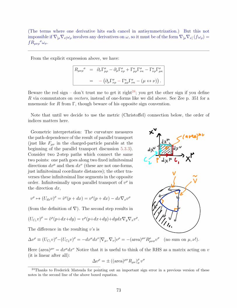
(The terms where one derivative hits each cancel in antisymmetrization.) But this notimpossible if∇[µ∇ν]ωρ involves any derivatives on ω, so it must be of the form∇[µ∇ν] (fωρ) =fRµνρ

σωσ.

From the explicit expression above, we have:

Rµνρσ = ∂νΓ

σµρ − ∂µΓσνρ + ΓκµρΓ

σνκ − ΓκνρΓ

σµκ

= −(∂µΓσνρ − ΓκµρΓ

σνκ − (µ↔ ν)

).

Beware the red sign – don’t trust me to get it right24; you get the other sign if you defineR via commutators on vectors, instead of one-forms like we did above. See Zee p. 351 for amnemonic for R from Γ, though beware of his opposite sign convention.

Note that until we decide to use the metric (Christoffel) connection below, the order ofindices matters here.

Geometric interpretation: The curvature measuresthe path-dependence of the result of parallel transport(just like Fµν in the charged-particle parable at thebeginning of the parallel transport discussion 5.3.3).Consider two 2-step paths which connect the sametwo points: one path goes along two fixed infinitesimaldirections dxµ and then dxν (these are not one-forms,just infinitesimal coordinate distances); the other tra-verses these infinitesimal line segments in the oppositeorder. Infinitesimally upon parallel transport of vρ inthe direction dx,

vρ 7→ (Udxv)ρ = vρ(p+ dx) = vρ(p+ dx)− dx∇xvρ

(from the definition of ∇). The second step results in

(UC1v)ρ = vρ(p+dx+dy) = vρ(p+dx+dy)+dydx∇y∇xvρ.

The difference in the resulting v’s is

∆vρ ≡ (UC1v)ρ−(UC2v)ρ = −dxµdxν [∇µ,∇ν ]vρ = −(area)µνRρ

µνσvσ (no sum on µ, ν!).

Here (area)µν = dxµdxν Notice that it is useful to think of the RHS as a matrix acting on v(it is linear after all):

∆vρ = ± ((area)µνRµν)ρσ v

σ

24Thanks to Frederick Matsuda for pointing out an important sign error in a previous version of thesenotes in the second line of the above boxed equation.

73

Exercise: check this formula using the explicit Riemann tensor on S2 that you will find onproblem set 5, using the diagram at right: begin at the north pole and carry a south-pointingvector with you toward the equator; after an infinitesimal step south dθ, head east so thatyour longitude changes by dϕ, still carrying your south-pointing vector; then head back northand compare your south-pointing vector to the original one. [End of Lecture 9]

74

A word of warning about notation (which I failed to heed in a previous version ofthese notes): when studying tensors with multiple indices which are not symmetrized (suchas Rµνρ

σ), it is a good idea to keep track of the order of the indices, even when they aredistinguished by their height (i.e. σ is a covariant index and hence special in the previousexpression). This is so that if you have occasion to lower an index (as in e.g. Rµνρλ ≡Rµνρ

σgσλ) it is clear which of the now-all-lower indices is the one that began its life as an upperindex. If you want to TeX these things, this is accomplished by R_\mu\nu\rho^\sigma

rather than R_\mu\nu\rho^\sigma.

Properties of Rµνρσ: (The symmetry properties below are very useful – they reduce the

44 components of a general 4-index object down to just at-worst 20 independent componentsof R)

1. From the definition we see that Rµνρσ = −Rνµρ

σ.

2. If Γρ[µ,ν] = 0 then

0 = R[µνρ]σ ≡ Rµνρ

σ +Rνρµσ +Rρµν

σ

−Rνµρσ −Rµρν

σ −Rρνµσ

That is, R has ‘cyclic symmetry’.

Proof: For any one-form ω,

∇[µ∇ν]ωρno torsion

= Rµνρσωσ

=⇒ R[µνρ]σωσ = 2∇[µ∇νωρ] (62)

But ∇[µων] = ∂[µων] + Γρ[µ,ν]︸︷︷︸=T=0

so

R[µνρ]σωσ = 2∂[µ∂νωρ] = 2

(∂µ∂νωρ +∂ν∂ρωµ +∂ρ∂µων−∂ν∂µωρ −∂µ∂ρων −∂ρ∂νωµ

)= 0 (63)

3. Bianchi identity (not just algebraic):

∇[µRνρ]σδ = 0.

Notice its resemblance to 0 = εµνρσ∂νFρσ = (?dF )µ, which came from F = dA.

We will prove this statement later (in §6.0.6) using Riemann normal coordinates (sinceit’s a tensor equation, proving it in some special coordinate system suffices to showthat it’s a true statement about the tensor), once we know what those are. It alsofollows simply from the Cartan structure equations (§9.)

75

5.4.1 Whence the connection? (Christoffel gets it from the metric)

There are many rocks underneath which one can find connections. Any correspondencebetween tangent spaces at different points (linear, differentiable) does it. A nice one comesfrom the metric. This is called the Christoffel connection. It is determined by the tworeasonable demands:

• torsion-free: Γρ[µν] = 0.

• ‘metric-compatible’: ∇µgνρ = 0. The metric is covariantly constant. The wonderfulpractical consequence of this is: you can raise and lower indices without worryingabout whether you did it before or after doing the parallel transport or the covariantderivative.

Geometric interpretation: This is a very natural condition – it says that paralleltransport preserves the (proper) lengths of vectors, as well as angles between them, asfollows: v being parallelly transported in the εµ direction means

0 = vµ(x+ ε)− vµ(x+ ε) = ερ∇ρvµ .

– the first equality says that the vector v we get by parallel transport at x + ε is thevalue of the vector field at that point anyway, and the second is the definition of ∇.The change in the angle between v and w is proportional to

δ (v · w) = ερ∂ρ (v · w) .

But:

∂ρ(v · w) = ∂ρ (gµνvµwν)

It’s a scalar= ∇ρ (gµνv

µwν)Liebniz

= (∇ρgµν)︸ ︷︷ ︸=0

vµwν + gµν (∇ρvµ)wν + gµνv

µ (∇ρwν) (64)

So we see that δ (v · w) = ερ∂ρ (v · w) = 0.

Notice also that since the above are both differential conditions at a point, any confusionsI might have created about finite parallel transport drop out of our discussion.

76

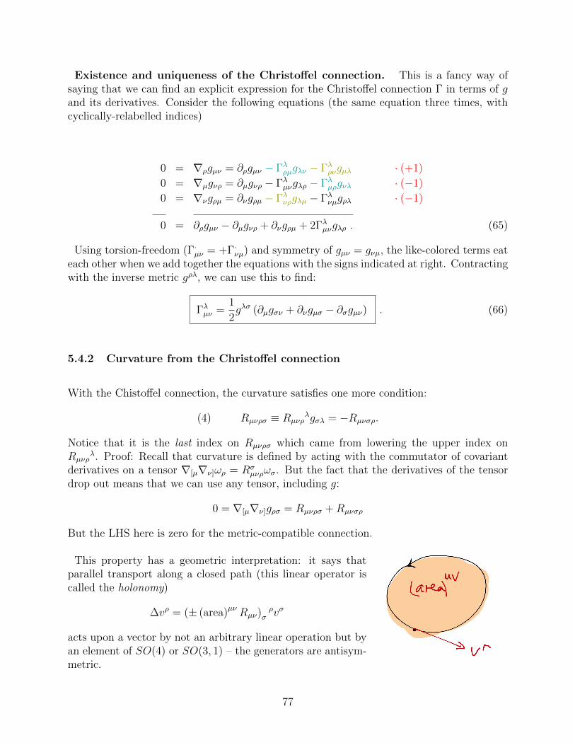
Existence and uniqueness of the Christoffel connection. This is a fancy way ofsaying that we can find an explicit expression for the Christoffel connection Γ in terms of gand its derivatives. Consider the following equations (the same equation three times, withcyclically-relabelled indices)

0 = ∇ρgµν = ∂ρgµν − Γλρµgλν − Γλρνgµλ · (+1)

0 = ∇µgνρ = ∂µgνρ − Γλµνgλρ − Γλµρgνλ · (−1)

0 = ∇νgρµ = ∂νgρµ − Γλνρgλµ − Γλνµgρλ · (−1)

0 = ∂ρgµν − ∂µgνρ + ∂νgρµ + 2Γλµνgλρ . (65)

Using torsion-freedom (Γ·µν = +Γ·νµ) and symmetry of gµν = gνµ, the like-colored terms eateach other when we add together the equations with the signs indicated at right. Contractingwith the inverse metric gρλ, we can use this to find:

Γλµν =1

2gλσ (∂µgσν + ∂νgµσ − ∂σgµν) . (66)

5.4.2 Curvature from the Christoffel connection

With the Chistoffel connection, the curvature satisfies one more condition:

(4) Rµνρσ ≡ Rµνρλgσλ = −Rµνσρ.

Notice that it is the last index on Rµνρσ which came from lowering the upper index onRµνρ

λ. Proof: Recall that curvature is defined by acting with the commutator of covariantderivatives on a tensor ∇[µ∇ν]ωρ = Rσ

µνρωσ. But the fact that the derivatives of the tensordrop out means that we can use any tensor, including g:

0 = ∇[µ∇ν]gρσ = Rµνρσ +Rµνσρ

But the LHS here is zero for the metric-compatible connection.

This property has a geometric interpretation: it says thatparallel transport along a closed path (this linear operator iscalled the holonomy)

∆vρ = (± (area)µν Rµν)σρvσ

acts upon a vector by not an arbitrary linear operation but byan element of SO(4) or SO(3, 1) – the generators are antisym-metric.

77

Notice that properties (4) and (3) imply

(5) Rµνρσ = Rρσµν .

While we’re at it we can define some other tensors that we can derive from the Riemanncurvature (the one with 4 indices):

Ricci tensor: Rµν ≡ Rµρνρ .

(Notice that this contraction is a weird one to consider from the point of view of the paralleltransport interpretation, but it’s still a tensor.)

Ricci scalar curvature: R ≡ Rµµ = gµνRµν .

Notice that the four tensors called R are distinguished by how many indices they have.

Einstein tensor: Gµν ≡ Rµν −1

2gµνR .

The reason to care about this combination is that it is “covariantly conserved” for any gµν :

0 = ∇µGνµ = ∇µGνµ.

Proof:Begin from Bianchi (not yet proved): 0 = ∇[µRνρ]σ

δ

contract with δµδ :

0 = ∇[µRνρ]σµ = 2

∇µRνρσµ +∇ν Rρµσ

µ︸ ︷︷ ︸=Rρσ

−∇ρRνµσµ︸ ︷︷ ︸

=Rνσ

and now contract with gνσ:

0 = ∇µRρµ +∇νRρ

ν −∇ρR = 2∇µGµρ .

(This is necessary if we’re going to set Gµν ∝ Tµν with Tµν a (covariantly) conserved stresstensor.)

WRAP-UP OF COVARIANT DERIVATIVE DISCUSSION

So the covariant derivative defines a notion of parallel for two vectors at different points.

Properties of ∇.

1. ∇ is a derivation.

2. The metric is covariantly constant: ∇ρgµν = 0.

A bit of notation: occasionally it is useful to use the following notation for derivatives of atensor (e.g.) Xα:

∂µXα ≡ Xα,µ, ∇µXα ≡ Xα;µ.

78

6 Geodesics

We’ve already discussed several warmup problems for the study of geodesics in curved space-time (flat space, Minkowski spacetime, and in fact on problem set 4 you already studied thegeneral case), so this should be easy. Consider a parametrized path in a manifold:

x : IR → Ms 7→ xµ(s) (67)

and let x ≡ dxds

(s). The

length of the curve, ` =

∫ s1

s0

ds√|gµν xµxν |

is a geometric quantity – it is independent of the choice of coordinates xµ → xµ(x) and ofthe parametrization: s→ s(s) (assuming s′(s) > 0).

Given a curve x, this produces a number – it is a functional `[x]. A geodesic is a curvefor which `[x] is stationary under small variations of the curve. This variation (fixing thelocations of the endpoints δxµ(s0) = 0 = δxµ(s1)) is (assuming for the moment a spacelikecurve to avoid some annoying absolute values)

0 =∂S

∂xµ(s)∝ e(s)

d

ds

(1

e(s)gµν(x(s))xν

)− 1

2(∂µgρσ) xρxσ

where e ≡√gµν xµxν . (Recall that this is the same quantity from problem set 4.) This

doesn’t look covariant, but we can make it more manifestly so using ddsgµν(x(s)) = ∂ρgµν x

ρ

and

Γµρν =

1

2gρσ (gµσ,ν + gσν,µ − gµν,σ)

in terms of which

gµνΓρµσx

ρxσ =1

2(2∂ρgνσx

ρxσ − ∂νgρσxρxσ)

and finally the geodesic equation is

ed

ds

(1

exµ)

+ Γρµσx

ρxσ = 0.

The geodesic equation is formal and useless, but true. It is (I think) always better to plugin the form of the metric to ds rather than beginning with the geodesic equation. We canimprove its utility slightly by taking advantage as before of its reparametrization invariance

to make e(s) =√gµν

dxµ

dsdxν

dsindependent of s. (Notice that now I am using s and not s since

it is not arbitrary. We can make such a choice since under

s→ s(s), e(s)→ e(s) =

√gµν

dxµ

ds

dxν

ds=

√gµν

dxµ

ds

dxν

ds

ds

ds

79

so we just need to pick dsds

= 1e(s)

. As before, such a parametrization is called an affineparameter since any other parameter satisfying this condition is s = as+b, with a, b constants(this is an “affine transformation” of s). Notice that the affine parameter is the length sofar: ` =

∫ s1s0e(s)ds = (const)(s1 − s0). Note that for a null curve, ‘const’ here means ‘zero’.

So in an affine parametrization, the geodesic equation is

d

ds

(dxµ

ds

)+ Γρ

µσ

dxρ

ds

dxσ

ds= 0 (Affine geodesic equation).

25

IVP: Consider for a moment the geodesic equation as a 2d order nonlinear ODE withindependent variable s and dependent variables xµ, just like the Newton equation md2xµ

dt2=

F µ(x)e.g.= −ηµν∂νV (x). As in that case, if we specify (xµ, dxµ

ds) ≡ (xµ0 , v

µ0 ) ∈ (M,TxM) at

s = s0, then ∃! solution in a neighborhood s > s0. This geodesic may not be extendibleto s = ∞ – for example it might hit some singularity or boundary. If it is so extendible,then the geodesic is called complete. If ∀(xµ, vµ), the resulting geodesic is complete, thenthe manifold M is geodesically complete. [End of Lecture 10]

Some examples:

1. The unit two-sphere S2: ds2S2 = dθ2 + sin2 θdϕ2

=⇒ e =√gµν xµxν =

√θ2 + sin2 θϕ2.

Geodesics satisfy

0 =δ`

δθ= −e d

ds

1

egθθ︸︷︷︸=1

θ

+1

2∂θ sin2 θ︸ ︷︷ ︸

=sin θ cos θ

ϕ2

0 =δ`

δϕ=

d

ds

(1

egϕϕϕ

)=

d

ds

(sin2 θϕ

e

).

With the affine parametrization, we can set e = 1 (this is a spacelike manifold, so theconstant can’t be zero)

=⇒ 0 =d

ds

(sin2 θϕ

)the quantity in parenthesis is conserved, an integral over the motion. This happenedbecause the metric was independent of ϕ – there is an isometry generated by the vector

25A point I under-emphasized in lecture is that this choice of affine parametrization e = 0 is consistentwith the geodesic equation, in the sense that if we make this choice at one value of s, the geodesic equationimplies that it continues to be true.

80

field ∂ϕ. (The conserved quantity is the z-component of the angular momentum. Infact there are two more conserved charges from the two other independent rotations,as you’ll see on problem set 5. Three conserved charges for a system with two dofsmeans the motion is completely integrable.)

2. Schwarzchild metric:

ds2Sch = −f(r)dt2 +

1

f(r)dr2 + r2

(dθ2 + sin2 θdϕ2

), with f(r) ≡ 1− r0

r

and r0 is a constant. If r0 → 0, this is Minkowski space. Notice that the 2-sphere fromthe previous example is what you get at fixed values of r and t, so the metric has theabove spherical symmetry. (Foreshadowing remarks: This solves Einstein’s equationswith Tµν = 0 for r > r0; with r0 = 2GM

c2, it describes a spherical object of mass M

centered at r = 0. You can see that some funny things happen at r = r0 and r = 0;those are topics for later and much later, respectively.)

For now, let’s consider a particle moving in the θ = π/2 plane (in fact this is WLOGby 3d rotational symmetry of the metric).

θ =π

2=⇒ `[t(s), r(s), ϕ(s)] =

∫ s1

s0

ds

√f(r(s))t2 − r(s)2

f(r(s))− r2ϕ2

The metric is independent of t and of ϕ: ∂t and ∂ϕ generate isometries (time translationinvariance and azimuthal rotation invariance, respectively). The t and ϕ variations aregoing to give us conservation laws26:

0 =δ`

δt=⇒ f(r)t ≡ ε = const, ‘energy’

0 =δ`

δϕ=⇒ r2ϕ ≡ L = const, angular momentum.

In affine coords

−gµν xµxν = +f(r)t2 − r2

f(r)− r2ϕ2 = κ= const

This is three integrals of motion (ε, L, κ) for 3 dofs (t, r, ϕ), so we can integrate. Elim-inate t, ϕ in κ:

1

2r2 +

1

2

(1− r0

r

)(L2

r2+ κ

)=

1

2ε2

26In general, if gµν is independent of xµ for some µ, then

0 =d

ds(gµν x

ν)− 1

2∂µgρσx

ρxσ =d

ds(gµν x

ν)

so the momentum pµ = gµν xν is conserved. As you can see from the S2 example, not every isometry need be

so manifest – ∂µgνρ = 0 in some coordinate system is a sufficient condition for ∂µ to generate an isometry, butnot necessary. It is also not a tensor equation. More generally the condition is Killing’s equation, Lvg = 0.

81

This is the Newtonian equation for the conserved energy E = 12ε2 + const with a

potential which is

V (r) =1

2

(1− r0

r

)(L2

r+ κ

)=

1

2κ︸︷︷︸

const

−κr0

2r︸ ︷︷ ︸Newtonian grav potential

+1

2

L2

r2︸︷︷︸centripetal potential

−r0L2

2r3︸ ︷︷ ︸new stuff!

The last term is new – a deviation from the Newtonian potential, and hence a deviationfrom elliptical orbits! This implies a precession of the perihelion (the point of closestapproach), which was observed first for Mercury. If you can’t wait to hear more aboutthis, see Appendix 1 of Zee §VI.3, p. 371.

The rest of this section is somewhat miscellaneous: it is a discussion of various topics relatedto geodesics, which will improve our understanding of the notions of curvature and paralleltransport introduced in the previous section, and move us toward contact with physics.

6.0.3 Newtonian limit

[Weinberg, page 77] Reality check: suppose (1) |dxidλ| dx0

dλ(slow particles) and (2) gµν =

ηµν + hµν , |hµν | 1 (in a weak field27). Let’s look at the geodesic equation in this limit.Neglecting d~x

dτin favor of dt

dτ, the affine geodesic equation reduces to:

0 =d2xµ

dτ 2+ Γµ00

(dt

dτ

)2

.

Further, let’s assume (3) a time-independent (or weakly time-dependent) gravitational field,∂tgµν = 0, so

Γµ00 = −1

2gµν∂νg00

weak field= −1

2ηµν∂νh00 +O(h2)

where we usedgµν ' ηµν − hµν︸︷︷︸

≡ηµρηνσhρσ

+O(h2).

Using again g ∼ 0, Γ000 ∝ ∂th00 = 0 and we have

0 =d2xi

dτ 2− 1

2∇ih00

(dt

dτ

)2

,d2t

dτ 2= 0

– the second equation is the affine parametrization condition in this limit. Dividing the BHSby the constant dt

dτ, we get

d2~x

dt2=

1

2~∇h00 .

27You could ask me what I mean by |hµν | 1 in a coordinate invariant way. One thing to do to make ascalar is to contract the indices with the Minkowski metric |h|1 = ηµνhµν . Another is |h|2 =

√ηµνhνρηρσhσµ.

We could keep going.

82

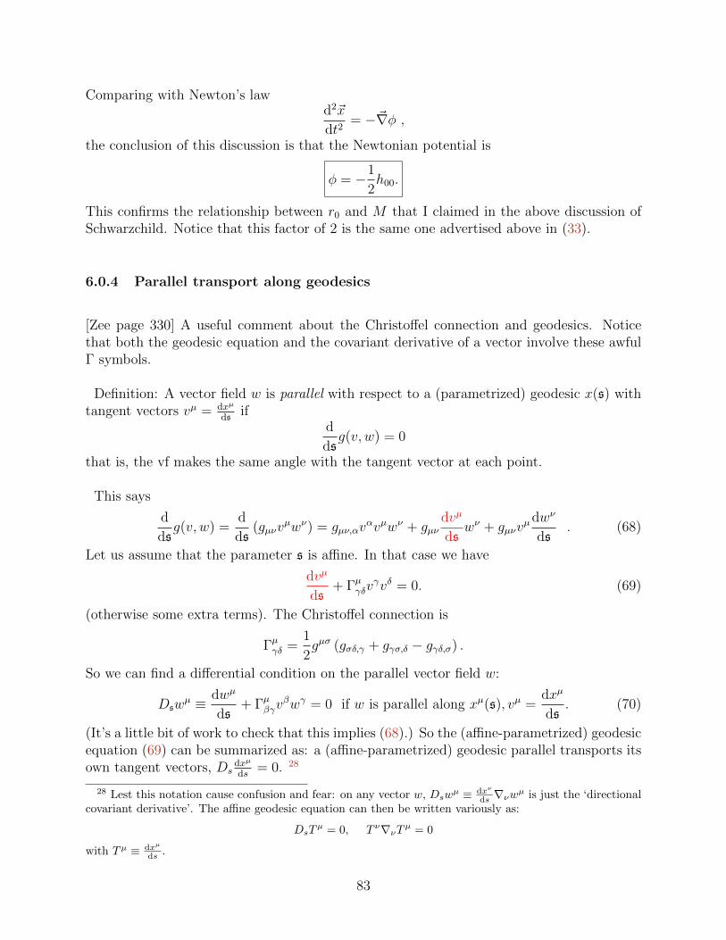
Comparing with Newton’s lawd2~x

dt2= −~∇φ ,

the conclusion of this discussion is that the Newtonian potential is

φ = −1

2h00.

This confirms the relationship between r0 and M that I claimed in the above discussion ofSchwarzchild. Notice that this factor of 2 is the same one advertised above in (33).

6.0.4 Parallel transport along geodesics

[Zee page 330] A useful comment about the Christoffel connection and geodesics. Noticethat both the geodesic equation and the covariant derivative of a vector involve these awfulΓ symbols.

Definition: A vector field w is parallel with respect to a (parametrized) geodesic x(s) withtangent vectors vµ = dxµ

dsif

d

dsg(v, w) = 0

that is, the vf makes the same angle with the tangent vector at each point.

This says

d

dsg(v, w) =

d

ds(gµνv

µwν) = gµν,αvαvµwν + gµν

dvµ

dswν + gµνv

µdwν

ds. (68)

Let us assume that the parameter s is affine. In that case we have

dvµ

ds+ Γµγδv

γvδ = 0. (69)

(otherwise some extra terms). The Christoffel connection is

Γµγδ =1

2gµσ (gσδ,γ + gγσ,δ − gγδ,σ) .

So we can find a differential condition on the parallel vector field w:

Dswµ ≡ dwµ

ds+ Γµβγv

βwγ = 0 if w is parallel along xµ(s), vµ =dxµ

ds. (70)

(It’s a little bit of work to check that this implies (68).) So the (affine-parametrized) geodesicequation (69) can be summarized as: a (affine-parametrized) geodesic parallel transports itsown tangent vectors, Ds

dxµ

ds= 0. 28

28 Lest this notation cause confusion and fear: on any vector w, Dswµ ≡ dxν

ds ∇νwµ is just the ‘directional

covariant derivative’. The affine geodesic equation can then be written variously as:

DsTµ = 0, T ν∇νTµ = 0

with Tµ ≡ dxµ

ds .

83

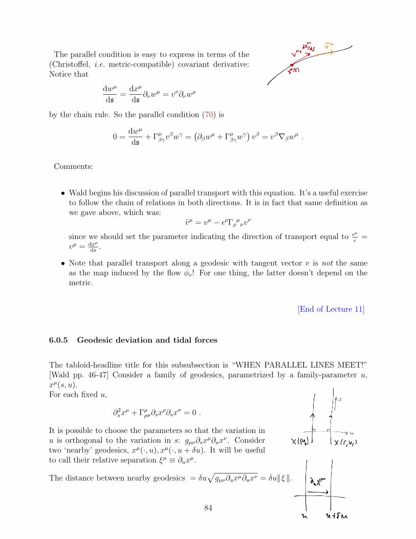
The parallel condition is easy to express in terms of the(Christoffel, i.e. metric-compatible) covariant derivative:Notice that

dwµ

ds=

dxµ

ds∂νw

µ = vν∂νwµ

by the chain rule. So the parallel condition (70) is

0 =dwµ

ds+ Γµβγv

βwγ =(∂βw

µ + Γµβγwγ)vβ = vβ∇βw

µ .

Comments:

• Wald begins his discussion of parallel transport with this equation. It’s a useful exerciseto follow the chain of relations in both directions. It is in fact that same definition aswe gave above, which was:

vµ = vµ − ερΓρµνvν

since we should set the parameter indicating the direction of transport equal to εµ

ε=

vµ = dxµ

ds.

• Note that parallel transport along a geodesic with tangent vector v is not the sameas the map induced by the flow φv! For one thing, the latter doesn’t depend on themetric.

[End of Lecture 11]

6.0.5 Geodesic deviation and tidal forces

The tabloid-headline title for this subsubsection is “WHEN PARALLEL LINES MEET!”[Wald pp. 46-47] Consider a family of geodesics, parametrized by a family-parameter u,xµ(s, u).For each fixed u,

∂2sx

µ + Γµρσ∂sxρ∂sx

σ = 0 .

It is possible to choose the parameters so that the variation inu is orthogonal to the variation in s: gµν∂sx

µ∂uxν . Consider

two ‘nearby’ geodesics, xµ(·, u), xµ(·, u + δu). It will be usefulto call their relative separation ξµ ≡ ∂ux

µ.

The distance between nearby geodesics = δu√gµν∂uxµ∂uxν = δu||ξ ||.

84

Let’s compute their acceleration toward each other. The vectorfield ξµ is not parallel transported in general; that is, theirrelative velocity is

vµ ≡ Dsξµ = ∂sξ

µ + Γµνρ∂sxνξρ 6= 0

(we introduced the notation Ds in (70) – recall that it just means Dswµ ≡ dxν

ds∇νw

µ). Moreinteresting is

aµ ≡ Dsvµ = DsDsξ

µ = ∂svµ + Γµρσ∂sx

νvσ = −Rνσρµ∂ux

ν∂sxσ∂sx

ρ.

For a derivation of the last step, see Wald p 47. You can see how there are two covariantderivatives involved; the derivation uses only the geodesic equation T µ∇µT

ν = 0, (T µ ≡ dxµ

ds),

and the fact that the Lie bracket [T, ξ] = 0.29

So this is another interpretation for the curvature: only if the curvature vanishes do initially-parallel geodesics remain parallel; a nonzero curvature measures the extent to which nearbygeodesics accelerate towards each other.

6.0.6 Riemann normal coordinates

[Zee page 343-344] The EEP guarantees that we can choose coordinates (i.e. go to an ap-propriate accelerating frame) which get rid of the gravitational force at any given point p(though not necessarily at any other points with the same choice!). From the previous dis-cussion, we see that this means that the Christoffel symbols vanish (at the chosen point) inthose coordinates: Γρµν(p) = 0.

I suppose that we must show this is actually possible mathematically; the fact that it’s aprinciple of physics means that it must be, if we are using the right mathematics! In any caseit is useful to know how to do it. A more formal definition of Riemann normal coordinates(ξ1, ...ξn) in a neighborhood of a point p ∈M is as follows. Given a tangent vector ξ ∈ TpM ,find an affine geodesic xξ(s) with the initial condition

xξ(s = 0) = p,dxµξds

(s = 0) = ξµ .

Then define the exponential map, exp : TpM →M as

exp(ξ) ≡ xξ(s = 1) ∈M .

29 For your convenience, I copy Wald (3.3.18) here:

aµ = T c∇c(T b∇bξµ

) [T,ξ]=0= T c∇c

(ξb∇bTµ

)product rule

= (T c∇cξb)∇bTµ + T cξb∇c∇bTµ[T,ξ]=0,def of R

= (ξc∇cT b)(∇bTµ) + ξbT c∇b∇cTµ −RcbdµξbT cT dproduct rule

= ξc∇c(T b∇bTµ)−RcbdµξbT cT dgeodesic eqn

= −RcbdµξbT cT d (71)

85

(If the manifold M is geodesically complete, the map exp is defined for any tangent vectorξ. Otherwise, we may have to limit ourselves to a subset Vp ⊂ TpM on which exp(ξ) isnonsingular. Since TpM ' IRn, its subspace V is an open subset of IRn.) We can then use aset of linearly independent vectors ξ(i) ∈ Vpni=1 to produce coordinates in the neighborhoodexp(Vp) of p which is the image of Vp.

On problem set 6 you will show that Γkij = 0 in this coordinate system. The basic ideais that straight lines in the tangent space (which is the coordinate space here) are mappedto geodesics by these coordinates. But the geodesic equation differs from the equation for astraight line by a term proportional to Γ.

Let’s Taylor expand the metric about such a point (p is x = 0) in such coordinates:

gτµ(x) = ητµ + gτµ,ν︸︷︷︸=0

xν +1

2gτµ,λσx

λxσ + ...

In the first term we have done a (constant) general linear transformation on our normalcoordinates to set gτµ(0) = ητµ. Notice that gτµ,λσ is symmetric under interchange of τ ↔ µor of λ↔ σ. Let’s plug this into our expression for the Christoffel symbols (66) (that we gotby demanding metric-compatibility):

Γλρν =1

2gλτ (gτν,ρ + gτρ,ν − gρν,τ ) = ηλτ (gτν,µρ + gτρ,µν − gρν,µτ )︸ ︷︷ ︸xµ + ... (72)

Plugging this into the expression for the R’n curvature we have30

Rµνρλ(p) = −∂µΓλνρ − (µ↔ ν) + ΓΓ︸︷︷︸

=0 at p

= −ηλτ (gτν,µρ + gτρ,µν − gρν,µτ ) +O(x)− (µ↔ ν) (73)

– at leading order in x, the ∂µ pulls out the (underbraced) coefficient of xµ in (72). Themiddle term is symmetric in µν drops out of the sum. For one thing, it makes manifest theantisymmetry in the last two indices: Rµνρσ = −Rµνσρ:

Rµνρσ = −gσν,µρ + gρν,µσ − (µ↔ ν) .

This is an explicit (tensor) expression for the R’n tensor which can be used to demonstratevarious of its properties. (Although we’ve derived the equation in specially-chosen coordi-nates, it is a tensor equation, so properties that we find in this coordinate system are justtrue.)

[Zee page 392, but beware that he puts the lowered index of R first!] Another is the Bianchiidentity, which we can see as follows. In general,

∇νRµσλρ = −∇ν

(∂µΓρσλ + ΓρκσΓκµλ − (µ↔ σ)

).

30Beware Zee’s notation for the order of the indices on the Riemann tensor. It is different from ours!

86

In R’n normal coords at p this simplifies to (Rµσλρ ≡ Rµσλαgαρ!)

∇νRµσλρ|p = ∂νRµσλρ|p =(∂ν∂σΓρ|µλ − ∂ν∂λΓρ|µσ

)|p

(here I have denoted ∂ν∂λΓρ|µσ ≡ gραΓαµσ to make clear which index is the lowered one). Nowif we cyclically permute the νσλ indices and add the three equations (like we did to derivethe expression for Γ in terms of g, but all with a + this time) we get

∇νRµσλρ =(∂ν∂σΓρ|µλ − ∂ν∂λΓρ|µσ

)∇σRµλνρ =

(∂σ∂λΓρ|µν − ∂σ∂νΓρ|µλ

)∇λRµνσρ =

(∂λ∂νΓρ|µσ − ∂λ∂σΓρ|µν

)∇νRµσλρ +∇σRµλνρ +∇λRµνσρ = 0

Like-colored terms cancel. This is the Bianchi identity. The version we wrote earlier

∇[νRµσ]λρ

is related to this one by property (5) Rµσλρ = Rλρµσ.

7 Stress tensors from the metric variation

Matter in curved space. We’ve already discussed the strategy for taking an action for aclassical field in Minkowski space (e.g. S =

∫d4xL(φ, ∂µφ) = −

∫d4x

(12∂µφ∂νφηµν + V (φ)

))

and turning it into an action in a curved metric gµν(x):

• Contract tensor indices with gµν instead of ηµν .

• Use the covariant measure d4x→ √gd4x.

This will produce an action for φ which is independent of coordinate choice, which reducesto the flat space action when g → η. Is it unique? No: for example we could add

SR ≡∫

d4x√g(ξRφ2 + ΥRµν∂µφ∂νφ+ ...

)where R is the Ricci scalar curvature... There are many terms, and the equivalence principledoesn’t decide for us the values of the coefficients. The dynamics in flat space does notuniquely determine the curved-space dynamics. The only consolation I can give you is thatby dimensional analysis nearly all of them are suppressed by some mass scale which seemsto be quite large.

Stress-energy tensor in curved space. Earlier, we applied the Noether method totranslation symmetry to find

T µflatν = − ∂L∂(∂µφ)

∂νφ+ δµνL

87

and in flat space ∂µTµν = 0 by the EoM. In curved space, we’ll find that:

T µcurvedν =1√g

(T µflatν + (improvements)µ ν) .

Using the equations of motion from the curved space action, the conservation law is covariantconservation:

∇µTµν = 0 .

Here is the better definition I promised (automatically symmetric, automatically has thesymmetries of S, differs from the old one only by improvement terms):

T µν(x) ≡ 2√g

δSmatter

δgµν(x).

Useful facts about derivatives with respect to elements of a matrix (for the next bit weforget that g depends on space):

∂

∂gµνdet g = (det g)gµν (74)

∂

∂gρσgµν = −gµρgνσ (75)

The second equation, (75), follows directly from varying gµνgνσ = δµσ . Note that we aredefining

∂gab∂gcd

= δcaδdb

– the fact that the metric is symmetric does not come into it.

Two proofs of (74):

•det g =

1

4!εabcdεmnpqgamgbngcpgdq

=⇒ δ det g =4

4!εabcdεmnpqgamgbngcp︸ ︷︷ ︸

=gdq det g

δgdq

where the underbraced equation follows from the cofactor expression for the inverse:

(A−1)ij = (−1)i+j1

detAdetA(ij)′

where A(ij)′ is the matrix obtained by removing the jth row and the ith column of A.

88

• For a symmetric matrix, (74) can be seen more usefully as follows, using the identity

det g = exp tr log g

What’s the log of a (symmetric) matrix? One way to define it is to Taylor expandabout the identity and use log(1 + x) = x− x2

2+ .... So if gab = ηab + hab then

(log g)ab = hab −1

2hach

cb +

1

3... .

A more robust understanding is as follows: A symmetric matrix can be diagonalized

g = U

λ1 0 · · ·0 λ2 · · ·0 0

. . .

U−1

with real eigenvalues λi. The log is then just

log g = U

log λ1 0 · · ·0 log λ2 · · ·0 0

. . .

U−1.

The det of g is the product of the eigenvalues: det g =∏

i λi, and tr log g =∑

i log λi.So

δ det g = etr log gδ (tr log g) = det gtrab (δ log g)ab = det gtrab(g−1δg

)ab

= det ggabδgab,

as claimed.

Putting back the position-dependence, we have

δgab(x)

δgcd(y)= δcaδ

db δ

4(x− y)

[End of Lecture 12]

Let’s apply the better definition of stress tensor to a scalar field with action

Smatter[φ, gµν ] = −1

2

∫d4x√g(gµν∂µφ∂νφ+m2φ2

)– I have highlighted the metric dependence. In Lorentzian signature, our notation

√g hides

the fact that √g ≡

√− det g

and therefore

δ√g = −1

2

1√gδ det g = − 1

2√ggabδgab det g =

1

2

√ggabδgab.

89

Using this,

2√g

δSmatter[φ, g]

δgab= 2

(1

2gacgbd∂cφ∂dφ−

1

4gab(gcd∂cφ∂dφ+m2φ

))which cleans up to the same expression we found previously:

Tab = ∂aφ∂bφ− gabL .

Similarly, you found on problem set 5 that E&M in curved space is described by the action

SEM [A, g] = − 1

16π

∫d4x√g gabgcdFacFbd︸ ︷︷ ︸

≡F 2

– notice that Fµν = ∂µAν − ∂νAµ does not involve any metric dependence.

T abEM =2√g

δ

δgab(x)SEM [A, g] =

−2

16π

(1

2gabF 2 − F a

cFcb

)=

1

16π

(4F a

cFcb − gabF 2

).

Finally, consider a point particle

Spp[x, g] = −m∫

ds√−gµν xµxν

T µνpp =2√g

δ

δgab(x)Spp =

∫dsδ4(x− x(s))

mxaxb√−gcdxcxd

which is what we got before using the trick of coupling to EM and demanding conservationof the total stress tensor.

Persnickety comments:

• Notice that the generally-covariant delta function satisfies:

1 =

∫d4y√g(y)δ4(y − x).

• Here’s how to remember the 2 in the definition: we’re only varying gµν and not itssymmetric partner gνµ when we take the derivative δ

δgµν. The 2 is meant to make up

for this.

90

• A warning about the sign [Zee page 380]: Notice that the sign in (74) implies that

Tµν =2√g

δSMδgµν

chain rule= −gµρgνσ

2√g

δSMδgρσ

– it’s not just the result of lowering the indices on 2√gδSMδgρσ

. The reason is that vary-

ing with respect to a component of the inverse metric is a different thing: δgρσ =−gρµδgµνgνσ– different things are held fixed when we do that.

8 Einstein’s equation

8.1 Attempt at a ‘correspondence principle’

So far we’ve been imagining that the metric gµν(x) is given to us by some higher power.Finally, we are ready to ask what determines the form of the metric, that is, we would liketo find the equations of motion governing it. What I mean by a ‘correspondence principle’is a guess based on the limit we know, namely the non-relativistic one.

In this limit, in a non-relativistic expansion about Minkowski spacetime, gµν = ηµν + hµν ,recall that we found above that the Newtonian potential was φ = −1

2htt. But the Newtonian

potential satisfies the Poisson equation, with the mass density as its source:

∇2φ = 4πGNρ . (76)

Let’s try to covariantize this equation.

ρ 7→ T00

∇2h00??7→ ∇2g00 ? No: ∇µgρσ = 0.

How about: ∇2h00??7→ R00 ? (77)

This might be good, sinceR·· ∼ ∂Γ + ΓΓ ∼ ∂2g + ∂g∂g

is a tensor which involves two derivatives of the metric. Demanding that (77) be the ttcomponent of a tensor equation would then give:

Rµν??= 8πGNTµν

A problem with this: the RHS is covariantly conserved, but the LHS is not! [Recall∂µ (maxwell)µ.]

The step (77) is ambiguous. With much hindsight we can see that we must use the(conveniently-named) Einstein tensor on the LHS instead,

Gµν?(yes)= 8πGNTµν

91

since we showed above that it satisfies

∇µGµν = 0 (Bianchi).

So this equation is compatible with covariant conservation of stress energy tensor, and (we’llsee later that it) reduces properly to the Newtonian limit31.

8.2 Action principle

What coordinate invariant local functionals of the metric and its derivatives are there? Bylocal functional again I mean we only get to integrate once. Let’s not allow too manyderivatives. Better: let’s organize the list by how many derivatives there are. It’s a shortlist:

Sgravity[g] =

∫dDx√g (a+ bR + ...)

Here I stopped at terms involving two derivatives. If we go to the next term (four derivatives),it’s:

Sgravity[g] =

∫dDx√g(a+ bR + c1R

2 + c2RµνRµν + c3R

····R···· + ...).

32

Dimensional analysis:[R] = [g−1∂Γ + g−1ΓΓ]

The first term is [R] = [g−1∂ (g−1∂g)] [a] ∼M4, [b] ∼M2, [c] ∼M0.

While we’re at it, let’s talk about units. You know that you can set c = 1 by measuringlengths in light-years. You can also set ~ = 1 by measuring energy in units of frequency (ormomenta in units of inverse length). You can set GN = 1 by measuring masses in units ofthe Planck mass, MPlanck, which as you can see from the above dimensional analysis will golike 1√

b= 1√

16πGN. That is, from GN , ~, c we can make a quantity with the dimensions of

mass

MPlanck ≡√

~c16πGN

.

(People disagree about the factors of 2 and π in this definition.) So we no longer need tochoose arbitrary systems of units for anything. ~, c, GN determined what units we shoulduse. For better or worse, MPlanck ∼ 1019GeV, so natural units are not so useful in mostlaboratories.

31 In four dimensions, the Einstein tensor is the only combination of the curvatures involving at most twoderivatives of the metric with this property. In higher dimensions there are other terms with these properties.

32Note that we are just studying the dynamics of gravity here, and not thinking yet about includingother matter, like the EM field. We’ll see how to include that very naturally below. The cosmological term(proportional to a) is a special case here.

92

For no good reason, let’s set a = 0. (FYI, it is called the ‘cosmological constant’.) Further,ignore c because it is suppressed by a large mass scale – if we are interested in smoothspacetimes where |R| Mhuge, then this is a good idea.

So I’m suggesting that we study

SEH[g] =1

16πGN

∫dDx√gR . (78)

This is called the Einstein-Hilbert action. I have renamed the constant b ≡ 116πGN

to beconsistent with convention.

We are going to show that

δSEH

δgµν(x)= +

1

16πGN

√g

(Rµν −

1

2gµνR

)= +

1

16πGN

√gGµν . (79)

First of all, we can see by easy considerations that the variation must be of the form

Rµν − αgµνR

for some constant α. [Zee page 347, argument that α 6= 14

: Zee page 350 ]

To proceed more systematically, we will collect some useful intermediate steps. Things thatare true:

1. The variation of the inverse of a matrix is related to the variation of the matrix by:δgµν = −gµαgνβδαβ. If we include the spacetime dependence:

δgµν(x)

δgαβ(y)= −gµαgνβδD(x− y)

2. δ√g = 1

2

√ggαβδgαβ Use log detM = tr logM .

δ√g(x)

δgαβ(y)=

1

2

√ggαβδD(x− y)

3. (δRµν) gµν = wα;α for some vector field wα.

Claim:δRµν = ∇ρ

(δΓρµν

)−∇µ

(δΓρρν

)where

δΓρµν =1

2gρσ (∇µδgνσ +∇νδgµσ −∇σδgµν)

93

where ∇ here is the covariant derivative with respect to the gµν about which we arevarying. Notice by the way that the extra term in the coordinate transformation of Γ(the badness in (60)) is independent of the metric, so δΓ is a tensor, and the aboveexpression includes the ΓΓ terms. (Alternatively, we can arrive at the same conclusionusing normal coordinates at any point p, in which case, at p

Rµν |p = Γαµν,α − Γαµα,ν ,

and the following steps are the same.)

Notice that this is

(δRµν) gµν = wα;α =

1√g∂α (√gwα) (80)

, by our formula for the covariant divergence.

4.∫

dDx√gwα;α = 0 if w has finite support. This is just IBP and the ordinary Gauss’/Stokes’

Thm.

Putting these together:

δSEH =1

16πGN

∫d4x

(−√g

(Rµν − 1

2Rgµν

)δgµν +

√ggµνδRµν

).

Neglecting the last term, which is a total derivative (by point 3 above), we have shown (79).

Comments:

• It is not an accident that δSEHδgµν

∝ Gµν is covariantly conserved – it is the Noether

current for translation invariance coming from the fact that SEH doesn’t depend onposition. That is: it’s the stress tensor for the metric.

• If we added higher-curvature terms, they would in general mess up the well-posednessof the Einstein equations as an initial value problem. There are certain combinationsof R2, RµνR

µν , R····R···· which does not produce 4-derivative terms in the action. They

appear in string theory sometimes and are named for Lovelock.

• If our space has a boundary, the boundary term produced by the variation of Rµν issignficant. If you need to worry about this, the keyword is ‘Gibbons-Hawking term’.

8.3 Including matter (the RHS of Einstein’s equation)

The variation of the action (78) gave just the LHS of Einstein’s equations. Given ourdiscussion of the right way to think about the stress tensor in section 7, including matter inEinstein’s equation is totally simple. Just add in the action for the matter:

S[g, stuff] = SEH [g] + SM [g, stuff].

94

Then the EoM for the metric are

0 =δS

δgµν(x)=

δSEHδgµν(x)

+δSMδgµν(x)

= − 1

16πGN

√gGµν +

√g

2T µν (81)

which saysGµν = 8πGNTµν ,

the Einstein equation.

Notice that this is a collection of n(n + 1)/2 = 10 in n = 4 dimensions nonlinear partialdifferential equations for the metric components, of which there are also a priori n(n +1)/2 = 10 components. The Bianchi identity is n = 4 ways in which the equations are notindependent, which matches the n = 4 coordinate transformations we can use to get ridof bits of the metric. Nonlinear means hard because you can’t just add solutions to findanother solution – no Fourier decomposition for you!

Notice that, if Tµν = 0, flat space gµν = ηµν is a solution.

8.3.1 The cosmological constant

[Zee page 356] For example: why did we leave out the constant term in the gravity action?Suppose we put it back; we’ll find an example of a stress tensor to put on the RHS ofEinstein’s equation. Then in the total action above,

SM = −∫

d4x√gΛ

where Λ is called the cosmological constant. Then the stress tensor on the RHS of Einstein’sequation is just

Tµν = Λgµν .

Notice that it is covariantly conserved because g is covariantly constant. (Notice also thatthere is no consequence of our decomposition of S into a matter action and a gravity action,so the ambiguity in where to put the cosmological constant is not a physics ambiguity.)

Notice that if Λ 6= 0, flat spacetime is not a solution of Einstein’s equations. The sign of Λmakes a big difference. (See problem set 8).

What is this Λ? Consider the case when there are scalar fields in the world. Then theirstress tensor looks like Tµν = ∂µφ∂νφ − gµνL. If we evaluate this in a configuration of thefield which is constant φ0 in spacetime, then we just get

Tµν = V (φ0)gµν

95

– so Λ = V (φ0), the value of the potential energy density. If we want the scalar to justsit there this value should probably be the minimum value of the potential. So we see thatthe additive normalization of our energy now really really matters. If there are multiplefields, the thing we care about is the total energy density. You might guess that the valueis determined by the highest energy scale of any physics that we have to include here. Sothis should include contributions from atomic physics ∼ (meV)4, from QCD ∼ (GeV)4, fromelectroweak physics ∼ (TeV)4, maybe from Grand Unified Theories ∼ (1016GeV)4 ? andmaybe from the Planck scale ∼ (1019GeV)4. However, the observed value is 122 orders ofmagnitude smaller than this, Λ ∼ +10−47GeV4.

As you’ll see on problem set 8, a positive cosmological constant produces a metric of theform

ds2FRW = −dt2 + a(t)2dxidxjδij

with a(t) = a0eHt and H ∼

√GNΛ – space expands exponentially fast. If the value of Λ

in our universe were even a little bit bigger, the universe would have expanded so quickly(compared to rates involved in particle interactions) that no galaxies would have formed,and things would have been very different then. Our colossal failure to explain its smallnesscombined with its crucial environmental role suggest that selection effects are responsible forits value. For more on this depressing but apparently correct line of thought, I recommendthis or (more complete but before the observation of nonzero Λ) this, describing Weinberg’s1988 prediction of its observed value from this perpective, and also this paper, describingthe mechanism (eternal inflation) by which values of Λ can be sampled.

[End of Lecture 13]

Next we will learn some useful math to help us recover from this crushing defeat.

96

9 Curvature via forms

The following is the way to compute curvatures if you have to do it analytically.

9.0.2 Vielbeins

We begin by introducing a new basis for vector fields and one forms.

Our previous basis for TpM was a coordinate basis: ∂∂Xµ , µ = 1, , dimM .

g

(∂

∂Xµ,∂

∂Xν

)= gµν 6= ηµν

– in general this is not an orthonomal basis (except in Riemann normal coords about p orin flat space). Their advantage is that

[∂

∂Xµ,∂

∂Xν] = 0.

New basis for TpM : tetrad basis:

ea, a = 1.. dimM

defined to be orthonormalg(ea, eb) = ηab. (82)

(I’ll use η to mean δ if we are in a space of euclidean signature. The letters a, b, c... run overthe orthonormal-basis elements.) These es are called vielbeins or n-beins or tetrads. Pricefor orthonormality: [ea, eb] 6= 0. But so what? See (83).

Expand these vectors in the old basis:

ea ≡ eµa∂

∂Xµ.

Similarly, we can expand the old basis vectors in the new basis:

∂µ = eaµea

(82)=⇒ gµν = ηabe

aµebν .

Notice that as matrices, the basis coefficients satisfy

“eaµ = (eµa)−1 ”, i .e. eaµeνa = δνµ, eaµe

µb = δab .

97

This basis for the tangent space produces a dual basis of one-forms:

θa, defined by θa(eb) = δab = 〈θa, eb〉

(just like dxν(

∂∂Xµ

)= δνµ).

In terms of these tetrad-basis one-forms, the metric is just

ds2 = θa ⊗ θbηab.

So these θs are easy to determine given an expression for the metric in coordinates.

Notation reminder (wedge product): From two one-forms θi, θj, we can define a section ofT ?M ⊗ T ?M , defined by its action on a pair of vector fields X, Y by(

θi ∧ θj)

(X, Y ) ≡ θi(X)θj(Y )− θj(X)θi(Y ).

It’s antisymmetric. This is called the wedge product.

Notation reminder (exterior derivative):

df = ∂ifdxi, dω = ∂iωjdxi ∧ dxj, dA(p) = cp∂[i1A

(p)i2...ip+1

dxi1 ∧ dxi2 ∧ · · · ∧ dxip+1

where cp is a conventional combinatorial factor. The operation d is designed so that d2 = 0.

9.0.3 The price of using an orthonormal frame

We defined the Riemann tensor as

[∇µ,∇ν ]ωρ = Rµνρσωσ

– in a coordinate basis for the tangent space. If we wanted to define the same object in amore general basis we need an extra term. For any two vector fields X, Y and one-form ω,let

R(X, Y )ω ≡(∇X∇Y −∇Y∇X −∇[X,Y ]

)ω .

(for any ω). In this expression ∇X ≡ Xµ∇µ is the directional covariant derivative along thevector field X. The earlier version of Riemann returns if we set X = ∂µ, Y = ∂ν , in whichcase the weird extra term goes away. Since this is true for all ω, we don’t need to write theω :

R(X, Y ) ≡ ∇X∇Y −∇Y∇X −∇[X,Y ] . (83)

The last, new term is required if we want R(X, Y ) to be a linear, non-differential operator,satisfying

R(X, Y )(fω) = fR(X, Y )ω

for any function f .

98

9.0.4 Connection and curvature in tetrad basis

Now consider∇Xeb

This is again a vector field and can be expanded in the new basis:

∇Xeb = ωba(X)ea

The ωba are called connection coefficients. They are one-forms – they eat a v.f. (X) to give

a number for each a, b. They contain the same data as the Γpmn33. Notice that

0 = ∇X 〈ea, eb〉︸ ︷︷ ︸=gab

= ωac(X)gcb + ωb

c(X)gac = ωab + ωba (84)

using metric-compatibility. This says that ω is antisymmetric in its two indices34.

Similarly the curvature tensor can be written by acting on the basis vectors, as:

R(X, Y )eb ≡ −(∇X∇Y −∇Y∇X −∇[X,Y ]

)eb = Ωb

a(X, Y )ea. (85)

(Note the extra sign because we are acting on a vector here, and not a one-form.) Thecurvature 2-forms Ω can be further expanded in our basis:

Ωba =

1

2Rcdb

aθc ∧ θd . (86)

In the tetrad basis, we have Rcdba = −Rdcb

a by construction, since the wedge is antisymmet-ric.

We can verify that this is consistent by taking the overlap with the tetrad-basis one-forms:

〈θa, R(ec, ed)eb〉(85)= 〈θa, Ωf

b (ec, ed)︸ ︷︷ ︸=Rghbfθg∧θf (eb,ec)

ef〉

(86)=

1

2〈θa, ef〉︸ ︷︷ ︸

=δaf

(Rcdb

f −Rdcbf)

=1

2(Rcdb

a +Rcdba) = Rcdb

a. (87)

Notice that we can also expand the curvature two forms in a coordinate basis for T ?pM :

Ωba =

1

2Ωµνb

adxµ ∧ dxν

33For the explicit connection between the connections see Zee page 60334Notice that I have lowered the second index – although these indices are raised and lowered with the

innocuous ηab, the antisymmetry of ω means we must be careful to distinguish ωab from ωba.

99

This lets us relate this fancy Ω thing to the components of the Riemann tensor in a coordinatebasis:

Rµνρσ = ebρe

σaΩµνb

a. (88)

Cartan structure equations. Here comes the payoff:

dθa + ωba ∧ θb = 0 (‘dθ + ωθ = 0’) (89)

Ωba = −dωb

a + ωbc ∧ ωca (‘R = −dω + ω2’). (90)

These allow us to calculate ω and Ω respectively, from which we can extract R using (86).

Eqn. (89) follows from torsion freedom of ∇, which can be written as the statement thatthe following vector field vanishes:

∇XY −∇YX − [X, Y ] = 0. (91)

Expand Y in our new basis: Y = θb(Y )eb. Then, from our expansion of ∇Xeb in the tetradbasis,

∇XY = X(θb(Y ))eb + θb(Y )ωba(X)ea

The torsion-free condition is then:

0(91)= (Xθa(Y ))ea−(Y θa(X))ea−θa([X, Y ])ea+

(ωb

a(X)θb(Y )− ωba(Y )θb(X))ea = 0 . (92)

Since the basis vectors are independent, each coefficient of ea must vanish independently:

0 = Xθa(Y )− Y θa(X)− θa([X, Y ])︸ ︷︷ ︸=dθa(X,Y )

+(ωb

a ∧ θb)

(X, Y )

The underbraced equation follows from the general statement:

Xω(Y )− Y ω(X)− ω([X, Y ]) = dω(X, Y ) , (93)

true for any vfs X, Y and one-form ω, which follows e.g. by writing it out in local coordinates.(This is sometimes taken as the definition of d.)

Pf of (90): This follows from the definition of the Riemann tensor

−Ωba(X, Y )ea = −R(X, Y )eb

=(∇X∇Y −∇Y∇X −∇[X,Y ]

)eb

= ∇X (ωba(Y )ea)−∇Y (ωb

a(X)ea)− ωba ([X, Y ]) ea= Xωb

c(Y )ec − Y ωbc(X)ec − ωbc ([X, Y ]) ec + ωba(Y )ωa

c(X)ec − ωba(X)ωac(Y )ec︸ ︷︷ ︸

=−ωba∧ωac(X,Y )ek

= (Xωbc(Y )− Y ωbc(X)− ωbc ([X, Y ]))︸ ︷︷ ︸

(93)= dωbc(X,Y )

ec − ωba ∧ ωac(X, Y )ec

= (dωbc − ωba ∧ ωac) (X, Y )ec (94)

100

which proves the second Cartan structure equation. (Beware that some sign conventionsdiffer between the above expressions and ones you will see in other sources.)

Sample application: IR2 in polar coordinates

step 1: demand that the metric is diagonal (δ or η) in the tetrad basis:

ds2 = dr2 + r2dϕ2 = θrθr + θϕθϕ.

Notice that I am using hats to indicate orthonormal-basis indices which are named aftercoordinate indices. From which we conclude that the tetrad basis is:

θr = dr, θϕ = rdϕ.

step 2: take derivatives. Since d2 = 0, we have

dθr = d2r = 0.

On the other hand, from (89) we have

dθr = −ωϕr ∧ θϕ

and there is no ωrr by (84). This means that ωϕ

r ∧ θϕ = 0 which means that ωϕr ∝ θϕ. And

by explicit computationdθϕ = d(rdϕ) = dr ∧ dϕ

while (i) saysdθϕ = −ωr ϕ ∧ θr = −ωr ϕ ∧ dr

from which we concludeωr

ϕ = dϕ

and all others vanish or are determined from it by symmetry. This is like knowing Γ.

step 3: Use (90) :Ωb

a = −dωba − ωca ∧ ωbc = 0

In this silly example we conclude that the curvature is zero.

Here is a less trivial example: Sample application: round S2 of radius R

ds2 = R2(dθ2 + sin2 θdϕ2

)= eθeθ + eϕeϕ

step 135:

=⇒ eθ = Rdθ, eϕ = R sin θdϕ = eϕϕdϕ.

35I’ve called the orthonormal one-forms e here while I called them θ earlier. Sorry.

101

step 2:

deθ = 0 = −ωϕθ ∧ eϕ =⇒ ωϕθ = −ωθ

ϕ ∝ eϕ.

deϕ = R cos θdθ ∧ dϕ =1

Rcot θeθ ∧ eϕ = −ωϕ

θ∧ eθ.

=⇒ ωθϕ =

1

Rcot θeϕ = −ωθ

ϕ, ωθθ = 0 = ωϕ

ϕ.

step 3:

Ωϕ

θ= −dωϕ

θ+ ωϕ

θ ∧ ωθϕ︸ ︷︷ ︸

∝eϕ∧eϕ=0

= −d (cos θdϕ) = + sin θdθ ∧ dϕ .

Using (88) we have

Rθϕθϕ = eθθ︸︷︷︸

=1

eϕϕ︸︷︷︸1/ sin θ

Ωθϕθϕ︸ ︷︷ ︸

− sin θ

=1

sin θ(+ sin θ) = 1.

andRθϕϕ

θ = eθθ︸︷︷︸

=1

eϕϕ︸︷︷︸sin θ

Ωθϕϕθ︸ ︷︷ ︸

− sin θ

= − sin2 θ

(and other nonzero components determined by symmetry) which is what we got usingChristoffel symbols on problem set 6.

[End of Lecture 14]

102

10 Linearized Gravity

[I recommend Carroll’s discussion of the subject of this chapter.] Now that we know whatequation to solve for the dynamical metric, we must look for solutions! In §12 we will discussthe Schwarzchild solution which describes the geometry created by a spherically symmetricmass distribution. Here we’ll ask a simpler question about solutions of Einstein’s equationswhich are nearly Minkowski space.

As we did earlier in §6.0.3, let’s consider linearizing about flat space (which is the onlysolution of Einstein’s equations that we know so far!):

gµν = ηµν + hµν , |h| 1, gµν = ηµν − hµν︸︷︷︸ηµαηνβhαβ

.

Everywhere in what follows “+O(h2) ” is implied. (If this makes you uncomfortable, imaginea little ε in front of every hµν .) Indices are raised and lowered with the Minkowski metric η.

Let’s plug this into Einstein’s equation, Rµν − 12gµνR = 8πGNTµν , again keeping only the

leading terms in h. First

Γρµν =1

2gρσ (gµσ,ν + gσν,µ − gµν,σ)︸ ︷︷ ︸

O(h)

=1

2ηρσ (hµσ,ν + hσν,µ − hµν,σ)

Rµνρσ = ∂νΓµρ|σ − ∂µΓνρ|σ − ΓΓ︸︷︷︸=O(h2)

=1

2(−hνσ,µρ + hµσ,νρ + hνρ,µσ − hµρ,νσ) .

Let h ≡ ηµνhµν ,2 ≡ ∂µ∂νηµν . Then

Rµν =1

2(∂µ∂νh+ ∂µ∂

ρhνρ + ∂ν∂ρhµρ −2hµν)

Gµν = Rµν −1

2Rgµν

= −1

2

(2hµν + ∂µ∂ρh

ρν + ∂ν∂ρh

ρµ − ∂µ∂νh− ηµν∂ρ∂σhρσ + ηµν2h

)Einstein

= 8πGNTµν . (95)

So this is a 2nd order linear differential equation, of the form

(Lh)µν = sourcesµν .

Here L is a 2nd order Laplace-like operator acting on symmetric rank-two tensor fields (Lis for ‘linear’ or ‘Lichnerowicz’).

103

Let’s compare to Maxwell’s equations (which are linear in A so no need to linearize):

∂µFµν = 2Aν − ∂ν∂µAµMaxwell

= 4πjν .

Again the LHS is of the form LA with L a 2d order linear differential operator acting ona tensor field, this time of rank 1. Notice that a gauge transformation Aµ → Aµ + ∂µλpreserves exactly this combination

2Aν − ∂ν∂µAµ → 2Aν − ∂ν∂µAµ + 2∂νλ− ∂ν∂µ∂µλ = 2Aν − ∂ν∂µAµ.

Similarly, we could have arrived at the above linearized Einstein equation (95) by demandingcoordinate invariance. That is, under (recall pset 7)

xµ → xµ + εµ(x), gµν → gµν − (∇µεν +∇νεµ) =⇒ hµν → hµν −

∂µ︸︷︷︸=∇ for g=η

εν + ∂νεµ

Under this replacement, Lh in (95) is invariant. So we could have begun the course withthe equation 2hµν = 0 (generalizing the Poisson equation for the Newtonian potential) andadded stuff to cancel the variations. This particle-physics-like point of view is taken in forexample the book by Weinberg and Feynman’s lectures on gravitation. From that point, youcan use this as the kinetic term for a free field with two indices and try to add interactionswhich preserve this invariance. The geometric approach we’ve taken is conceptually moreslippery perhaps, but much less hairy algebraically.

From our point of view now, the coordinate invariance is an annoying redundancy. Wecan use it to make our equation simpler. The same approach works well for Maxwell’sequations, where we could choose various gauge conditions, such as ‘temporal gauge’ A0 = 0(not Lorentz invariant but good for getting rid of minus signs) or ‘Lorentz gauge’ ∂µA

µ = 0.We’ll do the latter. This condition does not completely fix the redundancy since

Aµ → Aµ + ∂µλ =⇒ ∂µAµ → ∂µA

µ + ∂µ∂µλ

so λ with 2λ = 0 preserve our gauge condition (this ambiguity is removed by a choice ofinitial condition).

The GR analog of Lorentz gauge is “de Donder gauge”:

∂µhµν −1

2∂νh = 0. (96)

A linearized coordinate transformation

hµν → hµν − (∂µεν + ∂νεµ)

104

preserves the gauge condition (96) if

0 = 2εν + ∂µ∂νεµ −1

22∂ν∂

µεµ = 2εν .

Side remark. Note that (96) is the linearized definition of de Donder gauge. The nonlineardefinition is

0 = gµνΓρµν . (97)

You can check that this reduces to (96) if you linearize about Minkowski space. Note thatneither is a tensor equation, which is what we want in order to fix a property of our coordinatesystem. Under a nonlinear coordinate transformation xµ → xµ(x), (97) changes by

0 = gµνΓρµν → 0 = gµνΓρµν = gµνΓσµν∂σxρ − ∂µ∂ν xρgµν .

Requiring that (97) be true both before and after the transformation then restricts our choiceof coordinate transformations to those x(x) which satisfy

0 = ∂µ∂ν xρgµν = ∇µ∇µx

ρ = 2xρ(x)

– just like in the linearized case, the condition is that the transformation is harmonic.

• Note that the scalar box is

∇µ∇µ = gµν∂µ∂ν + gµνΓρµν︸ ︷︷ ︸(97)= 0

∂ρ = gµν∂µ∂ν .

• Notice that in nonlinear de Donder gauge,

∇µωµ = gµν(∂νωµ − Γρµνωρ

)= ∂µωµ

• Notice that we have treated xρ(x) as a scalar quantity here – they are just functions.

• gµνΓρµν = 0 is n conditions.

• If you find yourself in some coordinate system such that gµνΓρµν 6= 0, you can pick then functions xρ(x) such that

0 = gµνΓρµν = gµνΓσµν∂σxρ − ∂µ∂ν xρgµν ,∀ρ = 1..n

Back to linearized gravity. Imposing (linear) de Donder gauge ∂µhµν − 12∂νh = 0,

Gµν = −1

2

(2hµν −

1

2ηµν2h

)Einstein

= 8πGNTµν . (98)

105

In particular, in vacuum, Tµν = 0. Take the trace of both sides of (98), which gives 2h = 0(for n > 2). Plugging this back in gives

2hµν = 0

– gravitational waves !! Because the wave equation has nontrivial solutions, the metric in GRhas a life of its own, even away from any sources, just like the electromagnetic field. Restoringdimensionful quantities, you see that gravitational waves move at the speed of light. Thisis completely new compared to the Newton gravity theory where the gravitational field iscompletely determined by the mass distribution.

To understand these waves better, it is useful to define hµν ≡ hµν− 12ηµνh in terms of which

de Donder gauge is ∂µhµν = 0 and the Einstein equation (not in vacuum) is

2hµν = −16πGNTµν

which is just n2 copies of the Poisson equation.

(Notice that this bar operation (called ‘trace reversal’) squares to one in four dimensions.Rµν = Gµν − gµν

2Gρρ = 2hµν − 1

2ηµν2h = 2hµν . )

10.0.5 Newtonian limit.

Newton says: 1) ρ = T00 T0i, Tij – rest energy dominates. A nonrelativistic source is verymassive compared to its kinetic energy.

2) Stationary: no x0-dependence: 2 = −∂2t + ∆ = ∆.

2hµν = −16πGNTµνNR limit

∆h00 = −16πGNρ∆hi0 = 0∆hij = 0

The latter two equations are easy to solve (with suitable boundary conditions): hi0 = 0 = hij,which says

hij =1

2δijh, hi0 = 0, h = hµµ = −h00 + hii = −h00 +

3

2h =⇒ h00 =

1

2h

It remains to determine h:

h00 = h00 −1

2η00h = h00 +

1

2h =

1

2h+

1

2h = h.

=⇒ ∆h00 = −16πGNρ = ∆h

106

Comparing to Newton’s equation ∆φ = 4πGNρ, we have h = −4φ, h00 = −2φ, gij = −2δijφ.Our solution is: gµν = ηµν + hµν which says

g00 = −1 + h00 = −(1 + 2φ)gij = δij + hij = (1− 2φ)δijgi0 = 0

.

or more compactly

ds2φ = gµνdx

µdxν = −(1 + 2φ(~x))dt2 + (1− 2φ(~x))d~x · d~x

with ∆φ(~x) = +4πGNρ(~x) (Poisson). (99)

Notice: (1) There’s a nontrivial spatial component. So, although φ(x) satisfies the sameequation as in the Newtonian gravity, it produces twice as much bending of light in Einstein’stheory!

(2) As it must, since it solves the same equation, the Schwarzschild metric

ds2 = −(

1− 2GNM

r′

)dt2 +

1

1− 2GNMr′

dr′2 + r

′2ds2S2

is of this form to leading order in h, i.e. in GNM with φ = −GNMr

. This is becaused~x · d~x = dr2 + r2ds2

S2 where r′ and r differ by terms which are subleading in GNM . (Therelation is

(1− 2GNM

r′

)r2 ≡ r

′2.)

10.0.6 Gravitational radiation.

The existence of propagating wave solutions is something new and exciting that doesn’thappen in the Newtonian theory. This should be like the moment when you combinedAmpere’s and Faraday’s laws and found that there was light.

Put back the time derivatives:

2hµν = −16πGNTµν , 2 = −∂2t + ∆.

Even without sources, Tµν = 0, this has nontrivial solutions hµν(t, ~x). To solve 2hµν = 0,Fourier transform36:

hµν(x) =

∫d4kCµν(k)eik·x

(k · x ≡ kµxµ). Since we have linearized, we are studying a linear equation and can study it

mode-by-mode, so pick Cµν(k′) = Cµνδ(k − k′) for some k. So

0 = 2hµν = −k2Cµνeik·x (100)

36 d4k ≡ d4k(2π)4 , in direct analogy with ~ ≡ h

2π

107

requires k2 = 0 for a nontrivial solution, and we see that kµ = (ω,~k)µ means |ω| = |~k|, i.e.the waves propagate at the speed of light.

We arrived at the wave equation (100) by requiring de Donder gauge, and in momentumspace, this condition is

∂µhµν = 0 =⇒ kµCµν(k) = 0 .

There is also a residual gauge ambiguity (like in Lorentz-gauge E&M) – the de Dondergauge is preserved by xµ → xµ + εµ(x) if 2εµ = 0. This acts on h by

hµν → hµν − (∂µεν + ∂νεµ)

=⇒ hµν → hµν − (∂µεν + ∂νεµ − ηµν∂ρερ)

If εµ(x) = ε0µeik·x (everything is linear so we can study one momentum mode at a time) this

acts on the Fourier components by

=⇒ Cµν → Cµν − i(kµε

0ν + kνε

0µ − ηµνkρε0ρ

)– these two choices of C describe the same gravitational wave in (infinitesimally) differentcoordinates.

Altogether, the general solution for each wavevector kµ satisfying k2 = 0 is:

hµν(x) = Cµνeik·x,

with Cµν = Cνµ, kµCµν = 0,and Cµν ' Cµν + i (kµεν + kνεµ − ηµνk · ε) (101)

for any constant εµ.

How many components? That is – how many polarization states are there?

• Cµν = Cνµ symmetric 4-index object is 10.

• gauge condition kµCµν = 0 is 4 equations 10− 4 = 6.

• residual gauge equivalence εµ removes 4 more: 10− 4− 4 = 2.

(The analogous counting for Maxwell in Lorentz gauge: four possible polarizations Aµ(k)is n = 4, kµAµ(k) = 0 is one constraint n− 1 = 4− 1 = 3, and the residual gauge transf isAµ → Aµ + kµε removes one more: n− 2 = 4− 2 = 2 – same answer, different counting. Inother dimensions, these numbers aren’t the same. The photon always has n−2 polarizations.The graviton has n(n+2)

2− n− n = 1

2n(n− 3). Notice that this is zero in three dimensions.)

108

Explicitly, for any four-vector kµ = (ω,~k)µ with ω = ±|~k| pick axes so that ~k = (0, 0, ω).Then we can use our choice of ε and the condition kµCµν = 0 to write37

Cµν =

0 0 0 00 C+ C× 00 C× −C+ 00 0 0 0

µν

(102)

with C+ and C× parametrizing the independent polarizations (time is the first row of thematrix). (The names will be explained below.) A gravitational wave in this form is said tobe in “tranvserse, traceless” gauge; notice that with this choice hµν = hµν , since they differby a term proportional to the trace. [End of Lecture 15]

Comment on problem set 7 number 1 and problem set 8 number 3: this is a definition:φ(x) = φ(x) for the coordinate transformation of a scalar field. This is a statement ofinvariance: φ(x) = φ(x). For example, if x = x + ε, then this says φ(x) = φ(x − ε),that is: φ is constant. Similarly, gµν(x) = gµν(x) is an invariance statement. To testfor invariance, you have to compare the tensors at different points related by the allegedsymmetry transformation.

10.1 Gravitational wave antennae

Two questions we should address: (1) what do you feel if a gravitational wave of the form(101), (102) passes by you? (2) How are gravitational waves produced?

10.1.1 Receiver

(1) A single particle doesn’t care (a proof of this is the construction of Fermi normal coordi-nates which set the Christoffel symbols to zero along a whole geodesic; see Zee p. 557). Theinteresting thing is the resulting tidal forces between particles, as expressed in the geodesicdeviation equation. We (mostly) derived this earlier (in §6.0.5) and found that the relativeacceleration was determined by the Riemann tensor:

D2τξµ = Rνρσ

µξν∂τxρ∂τx

σ

where ξµ = ∂sxµ(τ, s) is the deviation vector describing the separation vector between two

nearby geodesics. Recall also that Dτ ≡ ∂τxµ∇µ. Let’s consider a collection of slow-moving

particles in our gravitational wave. Slow-moving means ∂τxρ ' (1,~0)ρ, and τ ∼ t, so the

geodesic deviation equation becomes

∂2t ξ

µ = Rνttµξν

37In words: we can use our n = 4 components of ε0µ to make Cµν traceless and and to make C0i = 0.

109

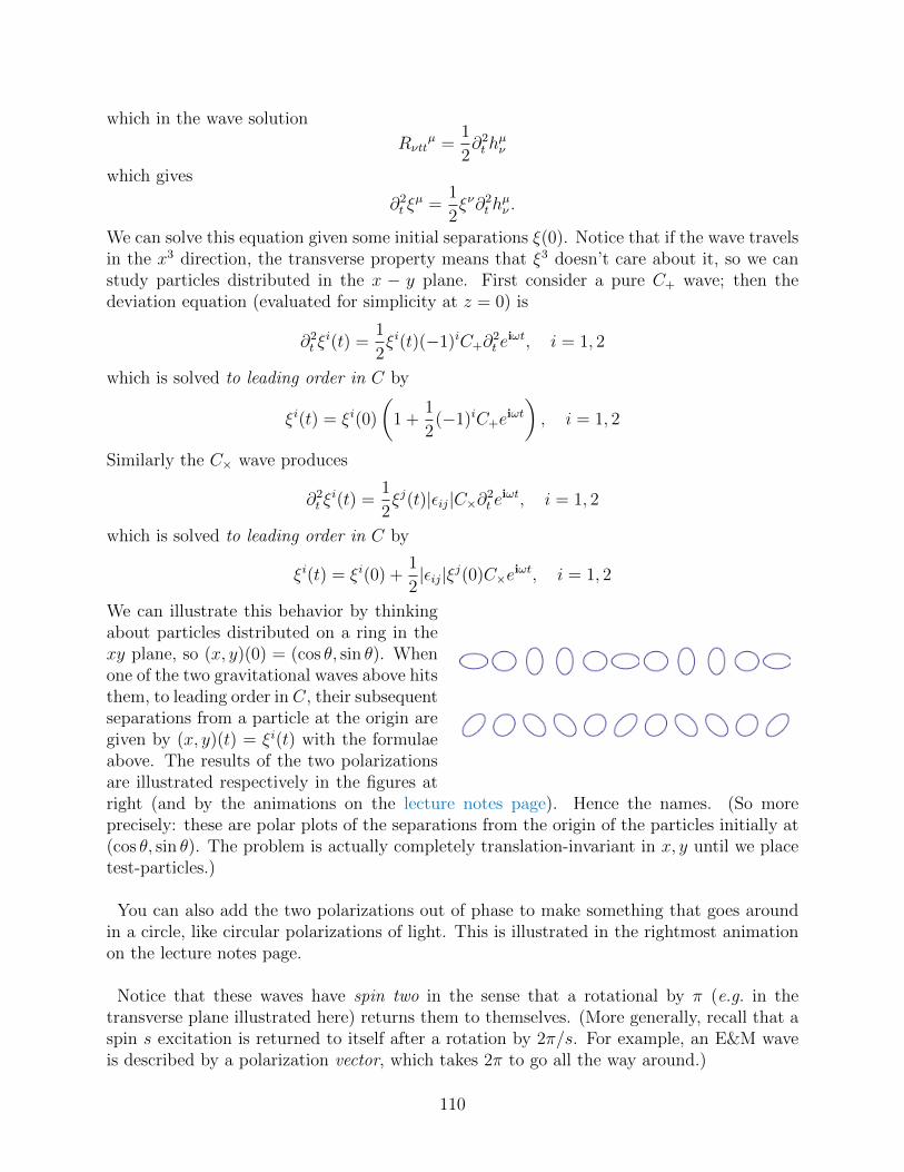
which in the wave solution

Rνttµ =

1

2∂2t h

µν

which gives

∂2t ξ

µ =1

2ξν∂2

t hµν .

We can solve this equation given some initial separations ξ(0). Notice that if the wave travelsin the x3 direction, the transverse property means that ξ3 doesn’t care about it, so we canstudy particles distributed in the x − y plane. First consider a pure C+ wave; then thedeviation equation (evaluated for simplicity at z = 0) is

∂2t ξ

i(t) =1

2ξi(t)(−1)iC+∂

2t e

iωt, i = 1, 2

which is solved to leading order in C by

ξi(t) = ξi(0)

(1 +

1

2(−1)iC+e

iωt

), i = 1, 2

Similarly the C× wave produces

∂2t ξ

i(t) =1

2ξj(t)|εij|C×∂2

t eiωt, i = 1, 2

which is solved to leading order in C by

ξi(t) = ξi(0) +1

2|εij|ξj(0)C×e

iωt, i = 1, 2

We can illustrate this behavior by thinkingabout particles distributed on a ring in thexy plane, so (x, y)(0) = (cos θ, sin θ). Whenone of the two gravitational waves above hitsthem, to leading order in C, their subsequentseparations from a particle at the origin aregiven by (x, y)(t) = ξi(t) with the formulaeabove. The results of the two polarizationsare illustrated respectively in the figures atright (and by the animations on the lecture notes page). Hence the names. (So moreprecisely: these are polar plots of the separations from the origin of the particles initially at(cos θ, sin θ). The problem is actually completely translation-invariant in x, y until we placetest-particles.)

You can also add the two polarizations out of phase to make something that goes aroundin a circle, like circular polarizations of light. This is illustrated in the rightmost animationon the lecture notes page.

Notice that these waves have spin two in the sense that a rotational by π (e.g. in thetransverse plane illustrated here) returns them to themselves. (More generally, recall that aspin s excitation is returned to itself after a rotation by 2π/s. For example, an E&M waveis described by a polarization vector, which takes 2π to go all the way around.)

110

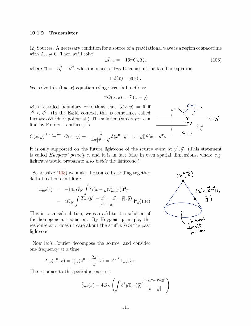
10.1.2 Transmitter

(2) Sources. A necessary condition for a source of a gravitational wave is a region of spacetimewith Tµν 6= 0. Then we’ll solve

2hµν = −16πGNTµν (103)

where 2 = −∂2t + ~∇2, which is more or less 10 copies of the familiar equation

2φ(x) = ρ(x) .

We solve this (linear) equation using Green’s functions:

2G(x, y) = δ4(x− y)

with retarded boundary conditions that G(x, y) = 0 ifx0 < y0. (In the E&M context, this is sometimes calledLienard-Wiechert potential.) The solution (which you canfind by Fourier transform) is

G(x, y)transl. inv.

= G(x−y) = − 1

4π|~x− ~y|δ(x0−y0−|~x−~y|)θ(x0−y0).

It is only supported on the future lightcone of the source event at y0, ~y. (This statementis called Huygens’ principle, and it is in fact false in even spatial dimensions, where e.g.lightrays would propagate also inside the lightcone.)

So to solve (103) we make the source by adding togetherdelta functions and find:

hµν(x) = −16πGN

∫G(x− y)Tµν(y)d4y

= 4GN

∫Tµν(y

0 = x0 − |~x− ~y|, ~y)

|~x− ~y|d3y.(104)

This is a causal solution; we can add to it a solution ofthe homogeneous equation. By Huygens’ principle, theresponse at x doesn’t care about the stuff inside the pastlightcone.

Now let’s Fourier decompose the source, and considerone frequency at a time:

Tµν(x0, ~x) = Tµν(x

0 +2π

ω, ~x) = eiωx

0Tµν(~x).

The response to this periodic source is

hµν(x) = 4GN

(∫d3yTµν(~y)

eiω(x0−|~x−~y|)

|~x− ~y|

)

111

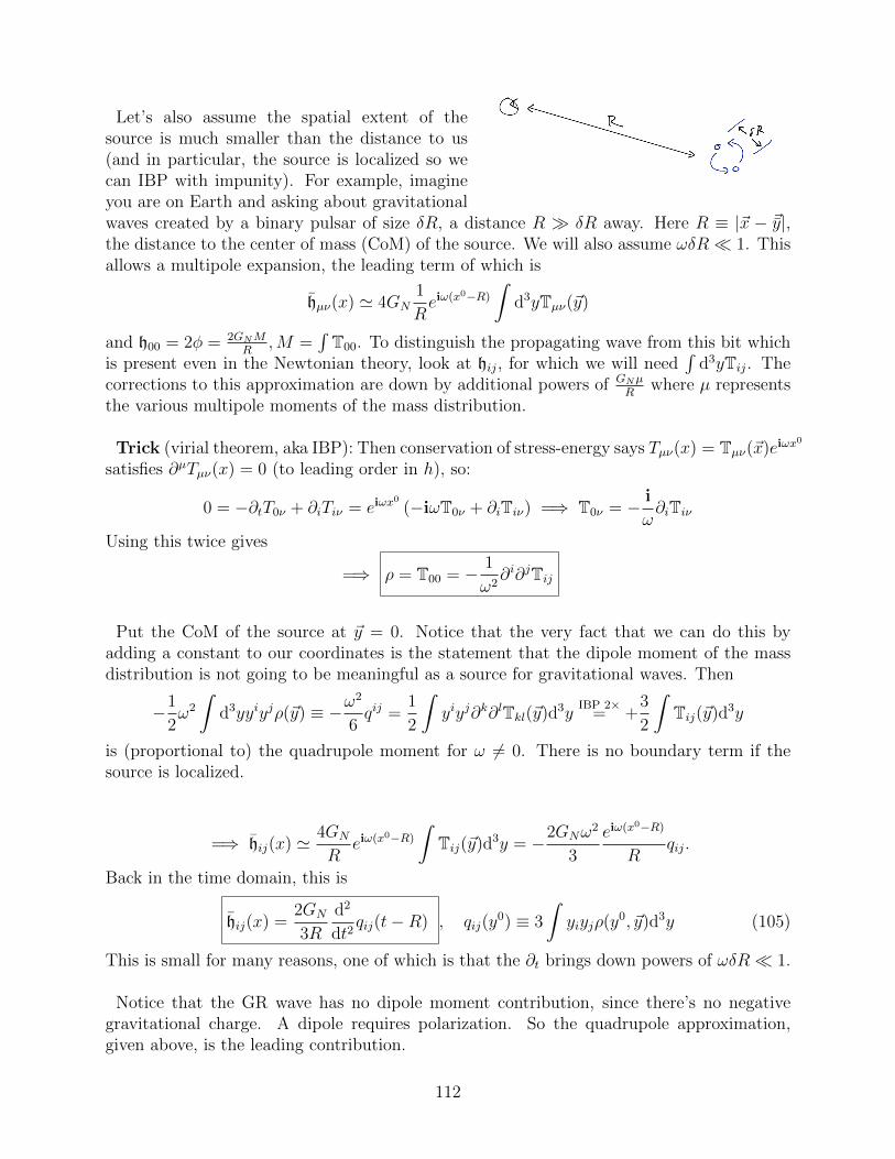
Let’s also assume the spatial extent of thesource is much smaller than the distance to us(and in particular, the source is localized so wecan IBP with impunity). For example, imagineyou are on Earth and asking about gravitationalwaves created by a binary pulsar of size δR, a distance R δR away. Here R ≡ |~x − ~y|,the distance to the center of mass (CoM) of the source. We will also assume ωδR 1. Thisallows a multipole expansion, the leading term of which is

hµν(x) ' 4GN1

Reiω(x0−R)

∫d3yTµν(~y)

and h00 = 2φ = 2GNMR

,M =∫T00. To distinguish the propagating wave from this bit which

is present even in the Newtonian theory, look at hij, for which we will need∫

d3yTij. Thecorrections to this approximation are down by additional powers of GNµ

Rwhere µ represents

the various multipole moments of the mass distribution.

Trick (virial theorem, aka IBP): Then conservation of stress-energy says Tµν(x) = Tµν(~x)eiωx0

satisfies ∂µTµν(x) = 0 (to leading order in h), so:

0 = −∂tT0ν + ∂iTiν = eiωx0

(−iωT0ν + ∂iTiν) =⇒ T0ν = − i

ω∂iTiν

Using this twice gives

=⇒ ρ = T00 = − 1

ω2∂i∂jTij

Put the CoM of the source at ~y = 0. Notice that the very fact that we can do this byadding a constant to our coordinates is the statement that the dipole moment of the massdistribution is not going to be meaningful as a source for gravitational waves. Then

−1

2ω2

∫d3yyiyjρ(~y) ≡ −ω

2

6qij =

1

2

∫yiyj∂k∂lTkl(~y)d3y

IBP 2×= +

3

2

∫Tij(~y)d3y

is (proportional to) the quadrupole moment for ω 6= 0. There is no boundary term if thesource is localized.

=⇒ hij(x) ' 4GN

Reiω(x0−R)

∫Tij(~y)d3y = −2GNω

2

3

eiω(x0−R)

Rqij.

Back in the time domain, this is

hij(x) =2GN

3R

d2

dt2qij(t−R) , qij(y

0) ≡ 3

∫yiyjρ(y0, ~y)d3y (105)

This is small for many reasons, one of which is that the ∂t brings down powers of ωδR 1.

Notice that the GR wave has no dipole moment contribution, since there’s no negativegravitational charge. A dipole requires polarization. So the quadrupole approximation,given above, is the leading contribution.

112

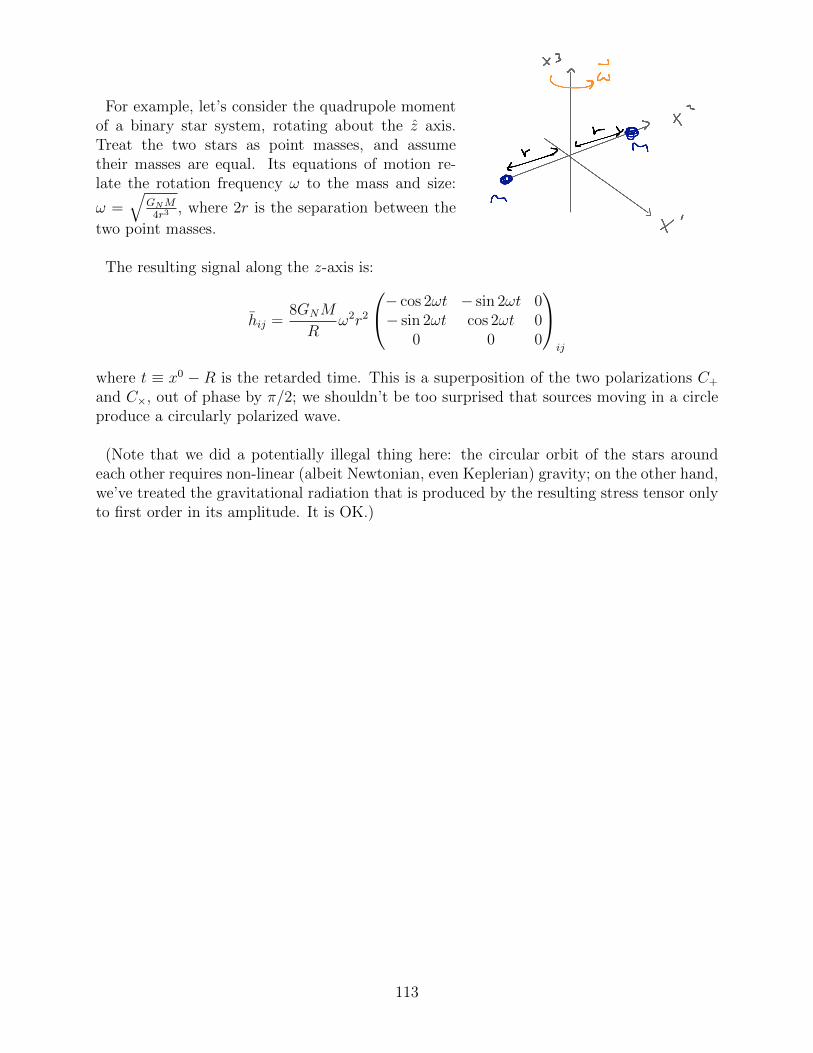
For example, let’s consider the quadrupole momentof a binary star system, rotating about the z axis.Treat the two stars as point masses, and assumetheir masses are equal. Its equations of motion re-late the rotation frequency ω to the mass and size:

ω =√

GNM4r3 , where 2r is the separation between the

two point masses.

The resulting signal along the z-axis is:

hij =8GNM

Rω2r2

− cos 2ωt − sin 2ωt 0− sin 2ωt cos 2ωt 0

0 0 0

ij

where t ≡ x0 − R is the retarded time. This is a superposition of the two polarizations C+

and C×, out of phase by π/2; we shouldn’t be too surprised that sources moving in a circleproduce a circularly polarized wave.

(Note that we did a potentially illegal thing here: the circular orbit of the stars aroundeach other requires non-linear (albeit Newtonian, even Keplerian) gravity; on the other hand,we’ve treated the gravitational radiation that is produced by the resulting stress tensor onlyto first order in its amplitude. It is OK.)

113

10.2 The gravitational field carries energy and momentum

Gravitational waves carry energy. How is this consistent with the idea that we can locallyeliminate the gravitational field, by the EEP? Well, the fact that we can’t eliminate agravitational wave by a coordinate change (recall that we used those up and were still leftwith two nontrivial polarization states for each (null) wavevector) already means that weare not in trouble with the EEP. The thing we can eliminate (locally) is a (locally) uniformgravitational field.

[End of Lecture 16]

But the definition of energy is quite tricky. The following discussion applies to the casewhere the spacetime is asymptotically flat – this means that far away, it looks like Minkowskispace. (This notion needs to be made more precise.) In this case, we can define a timecoordinate (a nice inertial frame at infinity), and define an energy associated with that timecoordinate. Here’s how the association works.

First define the energy-momentum tensor Tµν for the matter in a fixed geometry gµν(x)(with gµν(x)→ ηµν as x→∞) by the δS

δgµνprocedure from section 7. By problem set 7, we

have ∇µTµν = 0. Notice that this is not ∂µTµν = 0. Recall that in flat spacetime (i.e. inspecial relativity, as in (36)), we have

P µ =

∫Σt

T 0µd3~x

where Σt is a slice of spacetime at fixed time, i.e. what someone could consider ‘space’.

=⇒ ∂tPµ =

∫Σt

∂tT0µd3x

IF ∂µTµν=0= +

∫Σt

∂iTiµd3x =

∮∂Σt=∅

dsiTiµ = 0

– any change in the amount of conserved quantity in the region is accounted for by fluxthrough the boundary of the region. In curved spacetime, gµν(x), instead we have

∂tPµ ?

=

∫d3x

(∂iT

iµ − ΓµiαTiα − ΓiiαT

µα)

The first term can be Stokesed, but the Christoffel terms can’t. Also we haven’t used thecovariant integration measure. What about the more ideologically-correct object38

P µ ≡∫

Σt

d3x√gT 0µ

where Σt is a slice of spacetime at fixed time t? Now we have

∂µ (√gT µν )

∇µTµν=0=

1

2(∂νgρσ)

√gT ρσ

Einstein=

1

16πGN

(∂νgρσ)√g

(Rρσ − 1

2Rgρσ

).

38Notice that this is related to the construction you studied on problem set 8. If ξ = ∂t is a Killing vectorfield then in fact the Christoffel terms go away and the energy is conserved. In the case of a general solutionof the linearized equations, ∂t is a Killing vector field in the background Minkowski space, but not of thewave solution. The point is that energy can be exchanged between the gravitational field and matter.

114

(Notice that this does not contradict our claims (near (80)) about being about to integrateby parts with covariant derivatives because we are violating the assumption there that allthe indices are contracted.) This expression is somebody’s (ordinary) divergence:

∂µ (√gT µν ) = −∂µ (

√gtµν )

where

tµν ≡ 1

16πGN

((2ΓΓ− ΓΓ− ΓΓ) (gg − gg) + gµρgσκ (ΓΓ + ΓΓ− ...) + (µ↔ ν) + gg (ΓΓ− ΓΓ))

(106)is (a sketch of) the Landau-Lifshitz “quasi-tensor”39. So we have

∂µ (√g (T µν + tµν )) = 0

and can try to interpret the second term as the EM “tensor” for the gravitational field.But it can’t be a tensor because we could choose Riemann normal coordinates at p and setΓ|p = 0 =⇒ tµν |p = 0. So the gravitational energy is NOT a local concept, as expected bythe EEP.

If gravity is weak, gµν = ηµν + hµν , in de Donder gauge (∂µhµν = 0), this expressionsimplifies dramatically:

tµν =1

32πGN

∂µhρσ∂νhρσ (107)

Notice that this is manifestly O(h2), so we can consistently ignore the back-reaction of themetric on the gravitational wave at first order in h.

[Wald page 84] Here’s another way to think about this: the linearized Einstein equation is

G(1)µν [hρσ] = T (1)

µν

where the superscript indicates the order in the expansion in h. But this linearized solutionis not a solution to the next order; rather:

0 6= G(2)µν [hρσ] =

1

2hρσ∂µ∂νhρσ + ...

where ... is lots of other terms, all second order in h and which are what you get if I tell youwhere the indices go in (106) and you plug in the linearized solution to second order. Sothrough O(h2), the Einstein equation is

0 = (Gµν − 8πGNTµν) = 0 + s(G(1)µν [h]− 8πGNT

(1)µν

)+ s2

G(1)µν [h(2)] +G(2)

µν [h]− 8πGNT(2)µν︸ ︷︷ ︸

=−8πGNT totalµν

39Two confessions: This term ‘quasi-tensor’ is not standard. Wald and Landau-Lifshitz themselves call it a

‘pseudotensor’, but we’ve already used that term for tensors that get a minus sign under improper rotations.Also, the thing whose divergence is the expression above differs fro Landau and Lifshitz’ object by variousterms that don’t change the total energy, as explained a bit more in (108) below. The actual expression forthe LL quasi-tensor is equation (96.8) of volume II of Landau-Lifshitz. It has many indices!

115

where h(2) is the second-order correction to gµν = ηµν + shµν + s2h(2)µν + ... (and we have so

far assumed that Tµν = 0 in our linear study). So you see that we can interpret the secondorder equation as again Einstein’s equation but where the 1st order metric contributes tothe stress tensor at the next order:

T totalµν = T (2)

µν −1

8πGN

G(2)µν [h] .

So this is great, except for two problems:(1) The expression tµν is not actually gauge invariant. Under hµν → hµν +∂(µξν), it changes.Awful but inevitable. You knew this already from the dramatic simplification in de Dondergauge.(2) The replacement

tµν → tµν + ∂ρ∂σUµνρσ (108)

where U is local in h, quadratic in h, and satisfies symmetries similar to the Riemann tensor,Uabcd = U[ac]bd = Ubdac = Uac[bd] doesn’t change anything above.Consolations.(1) A virtue of the choice made by Landau-Lifshitz is that it only depends on first derivativesof g and is symmetric. They claim that it is the unique choice with these two properties.The reason we care that it is symmetric is that this makes the angular momentum, in theform

Mµν =

∫Σt

√g(xµT νttotal − xνT

µttotal

)conserved.

(2) Another consolation is that the LL quasi-tensor is a tensor under linear coordinatetransformations, in particular Lorentz transformations which preserve the Minkowski metricabout which we are expanding.

(3) A final consolation is that the total energy is invariant under ambiguities (1) and (2)(if the coordinate transformation ξ preserves the asymptotics). Supposing still that we havean asymptotically-flat spacetime, so that we have some canonical coordinates at ∞, with awell-defined spacelike hypersurface at each t, then

P µΣ =

∫Σ

(T µ0 + tµ0

)√gd3x

satisfies ddtP µ = 0 as usual:

d

dtP µ =

1

∆t

(∫Σt+∆t−Σt

√gd3x

(T µ0 + tµ0

))=

1

∆t

∫ t+∆t

t

dtd3x∂µ (√g (T µν + tµν))

Notice that this requires the matter to be localized (not extending to infinity), so thatT vanishes at ∞ and the Stokesing is justified. And in fact a more precise definition of

116

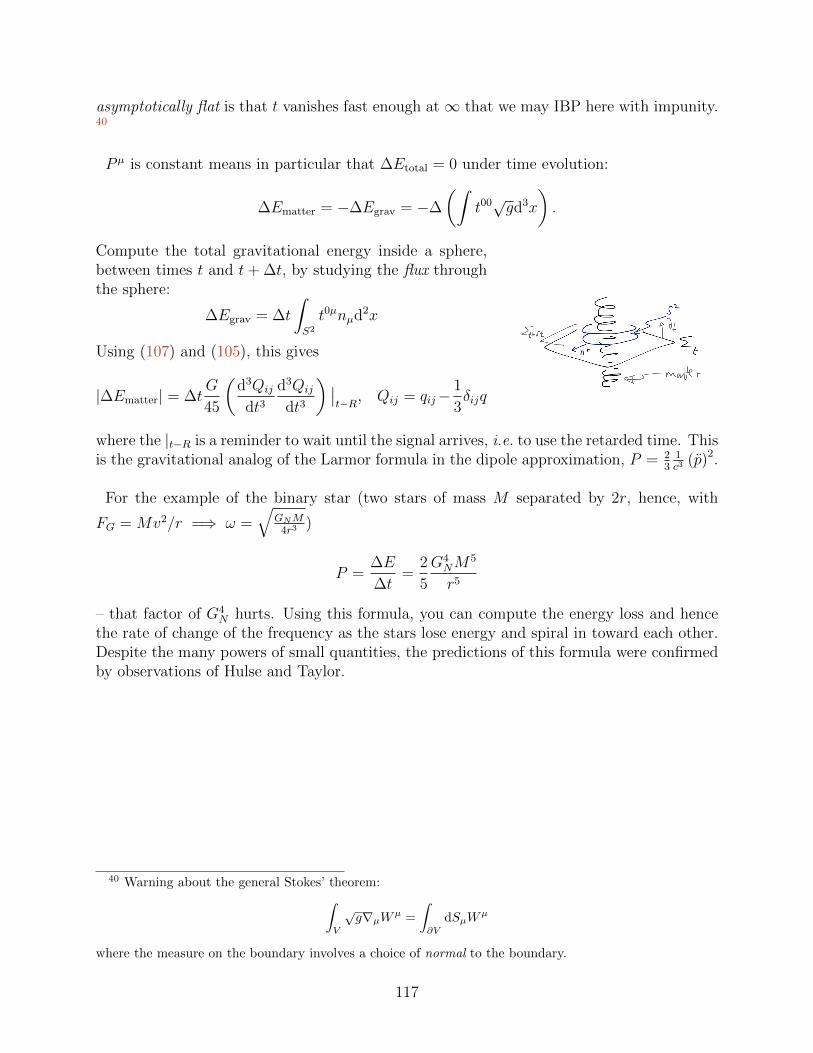
asymptotically flat is that t vanishes fast enough at∞ that we may IBP here with impunity.40

P µ is constant means in particular that ∆Etotal = 0 under time evolution:

∆Ematter = −∆Egrav = −∆

(∫t00√gd3x

).

Compute the total gravitational energy inside a sphere,between times t and t+ ∆t, by studying the flux throughthe sphere:

∆Egrav = ∆t

∫S2

t0µnµd2x

Using (107) and (105), this gives

|∆Ematter| = ∆tG

45

(d3Qij

dt3d3Qij

dt3

) ∣∣t−R, Qij = qij−

1

3δijq

where the |t−R is a reminder to wait until the signal arrives, i.e. to use the retarded time. Thisis the gravitational analog of the Larmor formula in the dipole approximation, P = 2

31c3

(p)2.

For the example of the binary star (two stars of mass M separated by 2r, hence, with

FG = Mv2/r =⇒ ω =√

GNM4r3 )

P =∆E

∆t=

2

5

G4NM

5

r5

– that factor of G4N hurts. Using this formula, you can compute the energy loss and hence

the rate of change of the frequency as the stars lose energy and spiral in toward each other.Despite the many powers of small quantities, the predictions of this formula were confirmedby observations of Hulse and Taylor.

40 Warning about the general Stokes’ theorem:∫V

√g∇µWµ =

∫∂V

dSµWµ

where the measure on the boundary involves a choice of normal to the boundary.

117

10.2.1 Exact gravitational wave solutions exist.

We have found wave solutions in perturbation theory about flat space (to leading order).There are also exact nonlinear solutions describing plane-fronted gravitational waves. Con-sider Minkowski space:

ds20 = −dt2 + dx2 + dy1dy1 + dy2dy2

and introduce lightcone coordinates u ≡ t+ x, v ≡ t− x so that

ds20 = −dudv +

∑i=1,2

dyidyi.

Consider the following deformation:

ds20 → ds2 = −dudv +

∑i=1,2

dyidyi + F (u, yi)du2. (109)

Here the function F is independent of v, but not necessarily small in any sense. Plug intothe vacuum einstein equations

Rµν −1

2gµν = 8πGNTµν = 0

the trace of which implies that R = 0 and hence Rµν = 0. I claim that with the ansatz (110)

Rµν = 0 ⇔∑i

∂2

∂yi∂yiF (u, y1, y2) = 0. (110)

(!) (110) is solved by

F (u, yi) =∑i,j=1,2

hij(u)yiyj if∑i

hii(u) = 0 .

so

(h)ij =

(h11 h12

h12 −h11

)which become the two linear polarizations C+, C× in the weak-field limit. This is called a‘plane-fronted wave’. It is a bit shocking that the dependence on u is completely uncon-strained; this is like for solutions of the 2d wave equation where you get to pick the initialwave profile.

[End of Lecture 17]

118

11 Time evolution

11.1 Initial value formulation

[Zee, §VI.6, p. 400] Recall our rough counting of degrees of freedom in GR. Let’s make thisa little more precise, and in particular, let’s imagine trying to teach a computer to solveEinstein’s equations. To do, so let’s back up to the beginning:

Particles. Recall Newton’s law for a particle mq = F (q, q). The fact that this equationis second order in time means you need to specify two initial conditions for each coordinateto determine a solution. Think of these as the initial position and initial momentum of theparticle. So, given q(t), q(t) at one time, we can determine their values at the next time stepq(t+ dt), q(t+ dt) by e.g.

q(t+ dt) = q(t) + dtq(t)

q(t+ dt) = q(t) + dtF (q(t),q(t))m

and you can do this again and again. Of course this can be optimized in many ways, buthere the point is the principle.

Fields. The above can be done also for many particles – just decorate with indices asappropraite:

mαβ qα = Fβ (q, q) .

A scalar field is just a collection of such variables where the label α includes spatial coordi-nates. No problem.

We could even be thinking about such fields in curved space. Notice that if we are beginningwith a covariant description, we have to pick a time coordinate along which to evolve.

Gauge fields. A small wrinkle arises if one is studying a system in a description involvinggauge redundancy. So consider E&M again: the four equations

∂µFµν = 4πjν

should determine Aµ(t + dt, x) given Aµ(t, x), ∂tAµ(t, x), jµ(t, x) right? In fact, they hadbetter not, because nothing can fix the gauge for us – that is, Aµ and Aµ ≡ Aµ + ∂µλ haveto give the same physics. So really we have only 4− 1 = 3 variables to solve for.

Happily, the ν = t equation is not an equation specifying the time evolution of anything.In more familiar langauge, it is the Gauss law constraint:

~∇ · ~E = 4πρ

which notice does not contain second time derivatives of Aµ. Rather, it is a constraint onpossible initial data – the charge density at time t determines the electric field at time t in

119

the familiar way. This means we have fewer equations (3) than we thought (4). But we alsohave fewer degrees of freedom (3) because the Aµ are determined by physics only up to a

gauge transformation. So initial data can be specified by ~A and its field momentum ~E = ∂L

∂ ~A,

subject to Gauss’ Law. Notice that if our initial data solves the Gauss law, the time-evolvedconfiguration does, too because

∂t

(~∇ · ~E − 4πρ

)= ~∇ ·

(∂t ~E

)︸ ︷︷ ︸

Ampere= ~∇× ~B−4π ~J

−4π ∂tρ︸︷︷︸continuity eqn

= −~∇· ~J

= 0.

So before we teach our computer to time-evolve our configuration of E&M fields, we haveto teach it to integrate the Gauss law at on our initial time slice.

Gravity. Now we have what seems like 10 equations

Gµν = Rµν − 1

2Rgµν = 8πGNT

µν

for what seems like 10 objects ∂2t gµν required to determine the metric components gµν(t +

dt, x) and its time derivatives ∂tgµν(t+ dt, x) at the next time step in terms of their presentvalues and the stress tensor T µν(x).

Again, the Einstein equations don’t determine this many quantities. By general covarianceof the Einstein equations, four objects must not be determined, since we can make the fourreplacements xµ → xµ(x).

And in fact, the four equations with a time index

Gtν = 16πGNTtν

are not evolution equations, but constraints, in that:Claim: Gtν does not contain ∂2

t gµν .Proof: (a) write it out explicitly and check.(b) Use ∇µG

µν = 0 to derive a contradiction – if there were second time derivatives in Gtν ,there would be third time derivatives in the quantity

∂tGtν = −∂iGiν + (Γ...G

..)ν

which you can see from the RHS of the identity there just aren’t. (Note that it does containterms like (∂tg..)

2, but this is useless for determining ∂2t g...)

Comments:

1. In a initial-value formulation, we are forced to distinguish the time coordinate. So wemight as well choose a gauge (like A0 = 0 gauge) where we get rid of gtµ, components

120

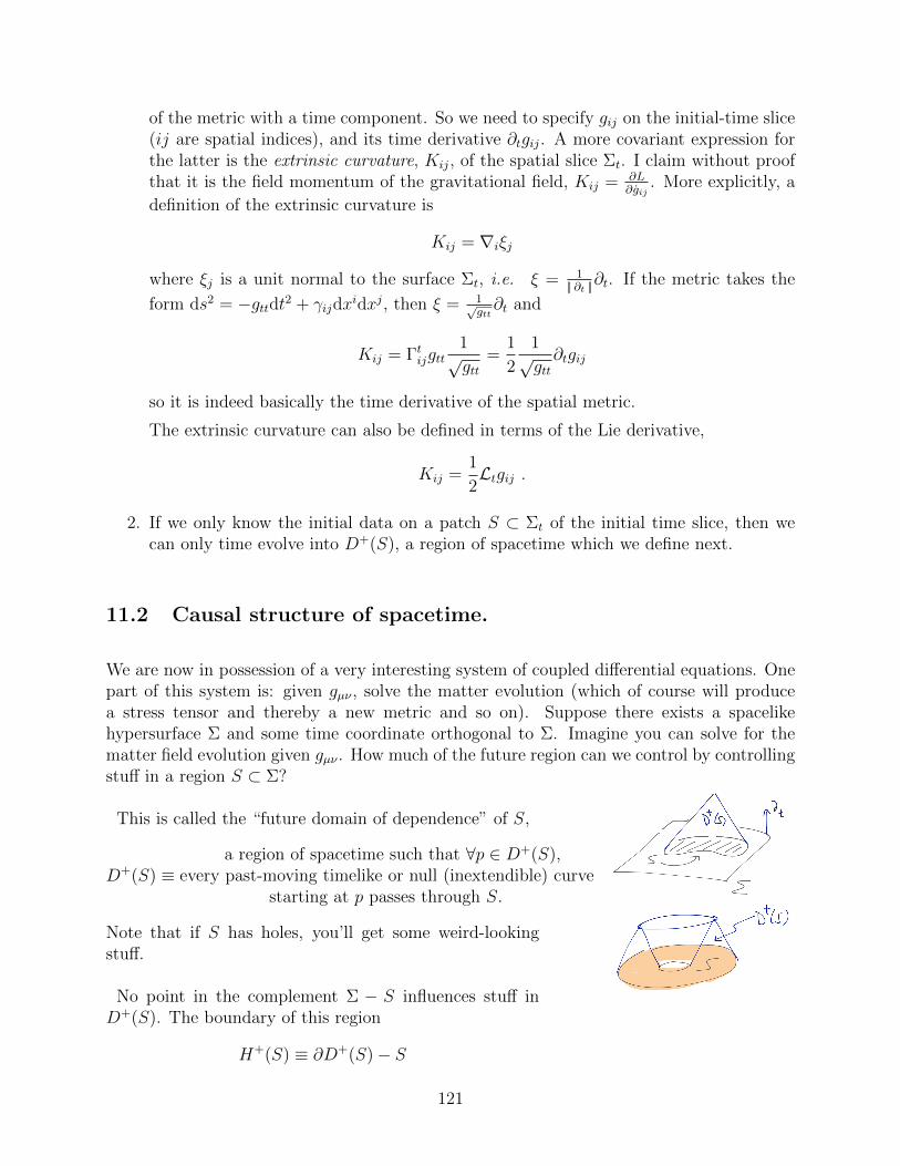
of the metric with a time component. So we need to specify gij on the initial-time slice(ij are spatial indices), and its time derivative ∂tgij. A more covariant expression forthe latter is the extrinsic curvature, Kij, of the spatial slice Σt. I claim without proofthat it is the field momentum of the gravitational field, Kij = ∂L

∂gij. More explicitly, a

definition of the extrinsic curvature is

Kij = ∇iξj

where ξj is a unit normal to the surface Σt, i.e. ξ = 1|| ∂t ||∂t. If the metric takes the

form ds2 = −gttdt2 + γijdxidxj, then ξ = 1√

gtt∂t and

Kij = Γtijgtt1√gtt

=1

2

1√gtt∂tgij

so it is indeed basically the time derivative of the spatial metric.

The extrinsic curvature can also be defined in terms of the Lie derivative,

Kij =1

2Ltgij .

2. If we only know the initial data on a patch S ⊂ Σt of the initial time slice, then wecan only time evolve into D+(S), a region of spacetime which we define next.

11.2 Causal structure of spacetime.

We are now in possession of a very interesting system of coupled differential equations. Onepart of this system is: given gµν , solve the matter evolution (which of course will producea stress tensor and thereby a new metric and so on). Suppose there exists a spacelikehypersurface Σ and some time coordinate orthogonal to Σ. Imagine you can solve for thematter field evolution given gµν . How much of the future region can we control by controllingstuff in a region S ⊂ Σ?

This is called the “future domain of dependence” of S,

D+(S) ≡a region of spacetime such that ∀p ∈ D+(S),

every past-moving timelike or null (inextendible) curvestarting at p passes through S.

Note that if S has holes, you’ll get some weird-lookingstuff.

No point in the complement Σ − S influences stuff inD+(S). The boundary of this region

H+(S) ≡ ∂D+(S)− S

121

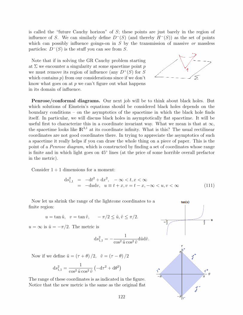
is called the “future Cauchy horizon” of S; these points are just barely in the region ofinfluence of S. We can similarly define D−(S) (and thereby H−(S)) as the set of pointswhich can possibly influence goings-on in S by the transmission of massive or masslessparticles: D−(S) is the stuff you can see from S.

Note that if in solving the GR Cauchy problem startingat Σ we encounter a singularity at some spacetime point pwe must remove its region of influence (any D+(S) for Swhich contains p) from our considerations since if we don’tknow what goes on at p we can’t figure out what happensin its domain of influence.

Penrose/conformal diagrams. Our next job will be to think about black holes. Butwhich solutions of Einstein’s equations should be considered black holes depends on theboundary conditions – on the asymptotics of the spacetime in which the black hole findsitself. In particular, we will discuss black holes in asymptotically flat spacetime. It will beuseful first to characterize this in a coordinate invariant way. What we mean is that at ∞,the spacetime looks like IR3,1 at its coordinate infinity. What is this? The usual rectilinearcoordinates are not good coordinates there. In trying to appreciate the asymptotics of sucha spacetime it really helps if you can draw the whole thing on a piece of paper. This is thepoint of a Penrose diagram, which is constructed by finding a set of coordinates whose rangeis finite and in which light goes on 45 lines (at the price of some horrible overall prefactorin the metric).

Consider 1 + 1 dimensions for a moment:

ds21,1 = −dt2 + dx2, −∞ < t, x <∞

= −dudv, u ≡ t+ x, v = t− x,−∞ < u, v <∞ (111)

Now let us shrink the range of the lightcone coordinates to afinite region:

u = tan u, v = tan v, − π/2 ≤ u, v ≤ π/2.

u =∞ is u = −π/2. The metric is

ds21,1 = − 1

cos2 u cos2 vdudv.

Now if we define u = (τ + θ) /2, v = (τ − θ) /2

ds21,1 =

1

cos2 u cos2 v

(−dτ 2 + dθ2

)The range of these coordinates is as indicated in the figure.Notice that the new metric is the same as the original flat

122

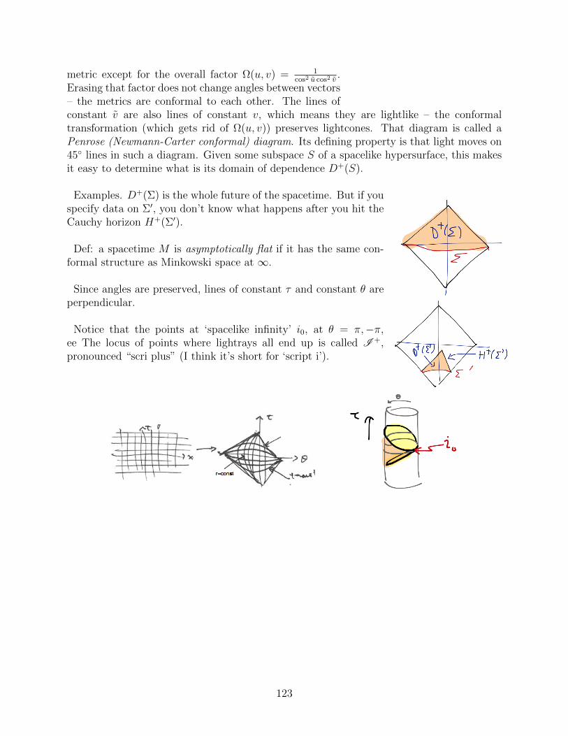
metric except for the overall factor Ω(u, v) = 1cos2 u cos2 v

.Erasing that factor does not change angles between vectors– the metrics are conformal to each other. The lines ofconstant v are also lines of constant v, which means they are lightlike – the conformaltransformation (which gets rid of Ω(u, v)) preserves lightcones. That diagram is called aPenrose (Newmann-Carter conformal) diagram. Its defining property is that light moves on45 lines in such a diagram. Given some subspace S of a spacelike hypersurface, this makesit easy to determine what is its domain of dependence D+(S).

Examples. D+(Σ) is the whole future of the spacetime. But if youspecify data on Σ′, you don’t know what happens after you hit theCauchy horizon H+(Σ′).

Def: a spacetime M is asymptotically flat if it has the same con-formal structure as Minkowski space at ∞.

Since angles are preserved, lines of constant τ and constant θ areperpendicular.

Notice that the points at ‘spacelike infinity’ i0, at θ = π,−π,ee The locus of points where lightrays all end up is called I +,pronounced “scri plus” (I think it’s short for ‘script i’).

123

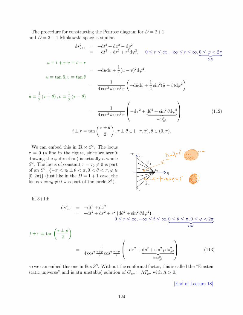
The procedure for constructing the Penrose diagram for D = 2+1and D = 3 + 1 Minkowski space is similar.

ds22+1 = −dt2 + dx2 + dy2

= −dt2 + dr2 + r2dϕ2, 0 ≤ r ≤ ∞,−∞ ≤ t ≤ ∞, 0 ≤ ϕ < 2π︸ ︷︷ ︸OK

u ≡ t+ r, v ≡ t− r= −dudv +

1

4(u− v)2dϕ2

u ≡ tan u, v ≡ tan v

=1

4 cos2 u cos2 v

(−dudv +

1

4sin2(u− v)dϕ2

)u ≡ 1

2(τ + θ) , v ≡ 1

2(τ − θ)

=1

4 cos2 u cos2 v

−dτ 2 + dθ2 + sin2 θdϕ2︸ ︷︷ ︸=ds2

S2

(112)

t± r = tan

(τ ± θ

2

), τ ± θ ∈ (−π, π), θ ∈ (0, π).

We can embed this in IR × S2. The locusτ = 0 (a line in the figure, since we aren’tdrawing the ϕ direction) is actually a wholeS2. The locus of constant τ = τ0 6= 0 is partof an S2: −π < τ0 ± θ < π, 0 < θ < π, ϕ ∈[0, 2π) (just like in the D = 1 + 1 case, thelocus τ = τ0 6= 0 was part of the circle S1).

In 3+1d:

ds23+1 = −dt2 + d~x2

= −dt2 + dr2 + r2(dθ2 + sin2 θdϕ2

),

0 ≤ r ≤ ∞,−∞ ≤ t ≤ ∞, 0 ≤ θ ≤ π, 0 ≤ ϕ < 2π︸ ︷︷ ︸OK

t± r ≡ tan

(τ ± ρ

2

)

=1

4 cos2 τ+ρ2

cos2 τ−ρ2

−dτ 2 + dρ2 + sin2 ρds2S2︸ ︷︷ ︸

=ds2S3

(113)

so we can embed this one in IR×S3. Without the conformal factor, this is called the “Einsteinstatic universe” and is a(n unstable) solution of Gµν = ΛTµν with Λ > 0.

[End of Lecture 18]

124

12 Schwarzschild black hole solution

Schwarzschild (‘black sign’), who discovered black holes even before Einstein figured outthe correct field equations (!) is someone we can add to our list of appropriately-namedphysicists (Poynting, Killing, Cutkowski, Cubitt, D’Eath and Payne, ...).

12.1 Birkhoff theorem on spherically-symmetric vacuum solutions

We will study solutions of the vacuum Einstein’s equations Gµν = 0. By trace-reversal, thisimplies Rµν = 0 – the spacetime is Ricci flat. The general solution is certainly not known(even in euclidean signature, it is not known; in that case, solutions include Calabi-Yaumanifolds which are useful in the context of string compactification). We will make twomore demands: we will demand that the spacetime be asymptotically Minkowski. And wewill demand spherical symmetry.

The solution we will find will also be static; that is a conclusion, not an assumption. Thismeans that the unique spherical solution we will find (given asymptotically-flat boundaryconditions) amounts to a GR generalization of Newton’s 20-year theorem on the gravita-tional effects outside a spherical mass distribution (it is called Birkhoff’s theorem). A usefulconsequence is: in a process of spherically-symmetric gravitational collapse, the solution wehave described is the correct solution at all times outside the region where the matter densityis nonzero. (The analogous thing happens in Maxwell theory: spherical symmetry impliesthat the vector potential is time-independent and the only solution is the Coulomb field.)

So we could start from the spherical and static ansatz

ds2 = r2(ds2

S2

)︸ ︷︷ ︸≡dθ2+sin2 θdϕ2

+e2b(r)dr2 − e2a(r)dt2

and just plug it into Rµν = 0, but the following is more instructive.

Symmetries of spacetime. What do we mean by a symmetry of spacetime (without apriori coordinates)? Given some metric gµν(x), its change at x under the flow generated bya vector field ξ is (problem set 8)

δgµν(x) = Lξgµν(x) = gµν(x)− gµν(x) = − (∇µξν +∇νξµ)

and if this vanishes then ξ is said to be a Killing vector field (Kvf) in that spacetime.Further claim: if ξ(1) and ξ(2) are Kvfs then so is their Lie bracket [ξ(1), ξ(2)]. So the Kvfsof a spacetime form a Lie algebra; exponentiating their action produces a Lie group whoseelements are the associated flow maps.

Spherical symmetry means that the manifold admits a set of three Kvfs ξ(a), a = 1, 2, 3

125

satisfying the so(3) Lie algebra:

[ξ(a), ξ(b)] = εabcξ(c)

that we found on the 2-sphere. By the Frobenius theorem (see Appendix B of Wald), theexistence of such Kvfs means that we can foliate the manifold by the orbits of the Kvfs,which in this case are S2s. If the manifold is 4-dimensional, this means that the metric mustbe of the form:

ds2 = ds2S2r2(a, b) + ds2(a, b)

– the coordinates a, b parametrize a two-dimensional family of two-spheres. In particular,there can be no dadθ cross-terms; that would require an SO(3)-invariant vector field v onthe S2 out of which to build da (vθdθ + vϕdϕ). Such a v does not exist.

Inexorable logic. From here it’s downhill to the Schwarzschild solution.• First, choose r(a, b) = r itself to be one of the two other coordinates. We are defining thecoordinate r to be the radius of the spherical sections (at fixed t). (Here “radius” meansthe r in the area = 4πr2.) You could worry that it’s not monotonic or all the spheres arethe same size, but this is not a real concern, since we will demand that asymptotically thesolution approach Minkowski space, where r is the radial polar coordinate. So the mostgeneral metric now is

ds2 = r2ds2S2 + gaa(r, a)da2 + 2gar(r, a)drda+ grr(r, a)dr2 .

(Notice that a must be the time coordinate.)

• We can get rid of the cross term by choosing t(a, r) appropriately.

Let’s argue backwards. Suppose we start with a metric of the diagonal form:

ds2 = −e−2α(r,t)dt2 + e2β(r,t)dr2

and change coordinates by t = t(a, r). Then

ds2 = −e−2α(r,t) (∂at)2 da2 − 2e2α(r,t)∂at∂rtdadr +

(e2β(r,t) − e2α(r,t) (∂rt)

2) dr2

So we can use the three freedoms α(r, t), β(r, t), t(a, r) to reproduce the previous grr(r, a), gar(r, a), gaa(r, a).

=⇒ ds2 = r2ds2S2 − e−2α(r,t)dt2 + e2β(r,t)dr2

• So far we have only used spherical symmetry and our ability to adapt our coordinatesto meet our needs. Now, finally, we impose Rµν = 0 on our choice of α(r, t), β(r, t). Thereisn’t really any good reason not to employ a computer to determine Γρµν [α, β] and therebyRµνρ

σ[α, β] and thereby Rµν [α, β]. A choice selection of components of the latter are:

Rtr =2

rβ (114)

126

Rθθ = e−2β(r,t) (r(β′ − α′)− 1) + 1 (115)

where ˙≡ ∂t,′≡ ∂r. So (114) immediately tells us that away from points where the sphere

shrinks to r = 0,β = 0 =⇒ β = β(r).

And then ∂t(115) implies

0 = e−2β (r∂t∂rα) =⇒ 0 = ∂r∂tα =⇒ α(r, t) = α(r) + γ(t).

• We can absorb this γ(t) into a redefinition of our time coordinate:

ds2 = −e2α(r,t)dt2 + · · · = −e2α(r) e2γ(t)dt2︸ ︷︷ ︸≡dt2

+ . . .

=⇒ dt

dt= eγ(t) =⇒ t(t) =

∫ t

dt′eγ(t′) .

Now drop the tildes and we are home: the most general spherically symmetric solution ofRµν = 0 has the form:

ds2 = r2(dθ2 + sin2 θdϕ2

)+ e2β(r)dr2 − e2α(r)dt2

So a spherically-symmetric solution of Rµν = 0 is also static. This means that there existcoordinates with ∂tgµν = 0 and no cross-terms: gµt = 0. (A spacetime is merely stationary ifgµt 6= 0 in coordinates where the metric is time-independent; the Kerr solution for a rotatingblack hole is an example of this. Fancier concise statement: stationary means merely thatthere exists a timelike Kvf; static means stationary and foliated by spacelike submanifoldsnormal to the Kvf.)

The demand of asymptotic flatness imposes the boundary conditions

α(r)r→∞→ 0, β(r)

r→∞→ 0 .

The remaining Ricci-flat equations are usefully organized into

0 = Rrr −Rt

t =2

r(α′ + β′) =⇒ ∂r (α + β) = 0 =⇒ α(r) = −β(r) + c︸︷︷︸

absorb into t→ e−ct

(116)So α(r) = −β(r). The final contentful equation is:

0 = Rθθ = e−2β (r (β′ − α′)− 1) + 1(116)= e2α (r(−2α′)− 1) + 1 = −∂r

(re2α

)+ 1

=⇒ re2α = r − r0 (117)

127

where r0 is an integration constant.

e2α(r) = 1− r0

r.

You can check that this also solves Rtt = 0 and Rrr = 0 independently41.

ds2sch = −

(1− r0

r

)dt2 +

1

1− r0r

dr2 + r2ds2S2

is the Schwarzschild metric. When r0 → 0, this is just Minkowski space. As we’ve seen, theconstant r0 is related to the mass of the source r0 = 2GNM by matching to the Newtonianlimit.

12.1.1 Appendix: tetrad method assuming spherical static ansatz

Assumptions: we’ll look for a solution of Einstein’s equations in vacuum Tµν = 0 (for r 6= 0)which is spherically symmetric and static. Ansatz:

ds2 = r2(ds2

S2

)︸ ︷︷ ︸=dθ2+sin2 θdϕ2

+e2b(r)dr2 − e2a(r)dt2.

In fact, this ansatz is completely general given the symmetry assumptions, as should be clearfrom the earlier discussion.

We want to find the functions a(r), b(r) by solving Einstein’s equations. We’re going toneed Rµν , R; let’s construct them using the tetrad formalism, Eqs (89), (90).

1. find ON basis:

θt = ea(r)dt, θθ = rdθ, θϕ = r sin θdϕ, θr = eb(r)dr.

2. Calculate connection one-forms ωba using the first Cartan structure equation (89):

dθa = −ωba ∧ θb .

dθt = a′(r)eadr ∧ dt = a′eae−be−aθr ∧ θt = −a′e−bθt ∧ θr

41For completeness, their form in the static ansatz is

Rtt = e2(α−β)(α′′ + (α′)2 − α′β′ + 2

rα′)

Rrr = −α′′ − (α′)2 + α′β′ +2

rβ′. (118)

128

=⇒ ωrt = a′e−bθt, ωθ

t ∧ θθ = 0, ωϕt ∧ θϕ = 0.

dθθ = dr ∧ dθ =1

re−bθr ∧ θθ = −1

re−bθθ ∧ θr =⇒ ωr

θ = −e−b

rθθ

dθϕ = sin θdr ∧ dϕ+ r cos θdθ ∧ dϕ =sin θ

re−bθr ∧ θθ +

cot θ

rθθ ∧ θϕ

=⇒ ωrϕ =

e−b

rθϕ, ωθ

ϕ =1

rcot θθϕ

3. Calculate the curvature two-forms with the second Cartan structure equation (90):

Ωba = −dωb

a + ωbc ∧ ωca

Ωrt = d

(a′e−bθt

)+ 0

– the ω ∧ ω terms all vanish either by antisymmetry of forms or by vanishing of ωs.

Ωrt =

(a′′ − a′b′ + a′2

)e−2bθr ∧ θt.

Ωθt = ωθ

r ∧ ωr t = −a′

re−2bθt ∧ θθ

Ωϕt = −a

′

re−2bθt ∧ θϕ

Ωθr = −d

(1

re−b)θθ − 1

re−bdθθ + ωθ

ϕ ∧ ωϕr

=b′

re−2bθr ∧ θθ.

Ωrϕ =

b′

re−2bθr ∧ θθ

Ωθϕ = (1− e−2b)r−2θθ ∧ θϕ.

Other nonzero components are determined by Ωba = −Ωa

b.

4. Extract the Riemann tensor using

Ωba = Rbcd

aθc ∧ θd

=⇒ Rtrtr =

(a′′ − a′b′ + a′2

)e−2b

129

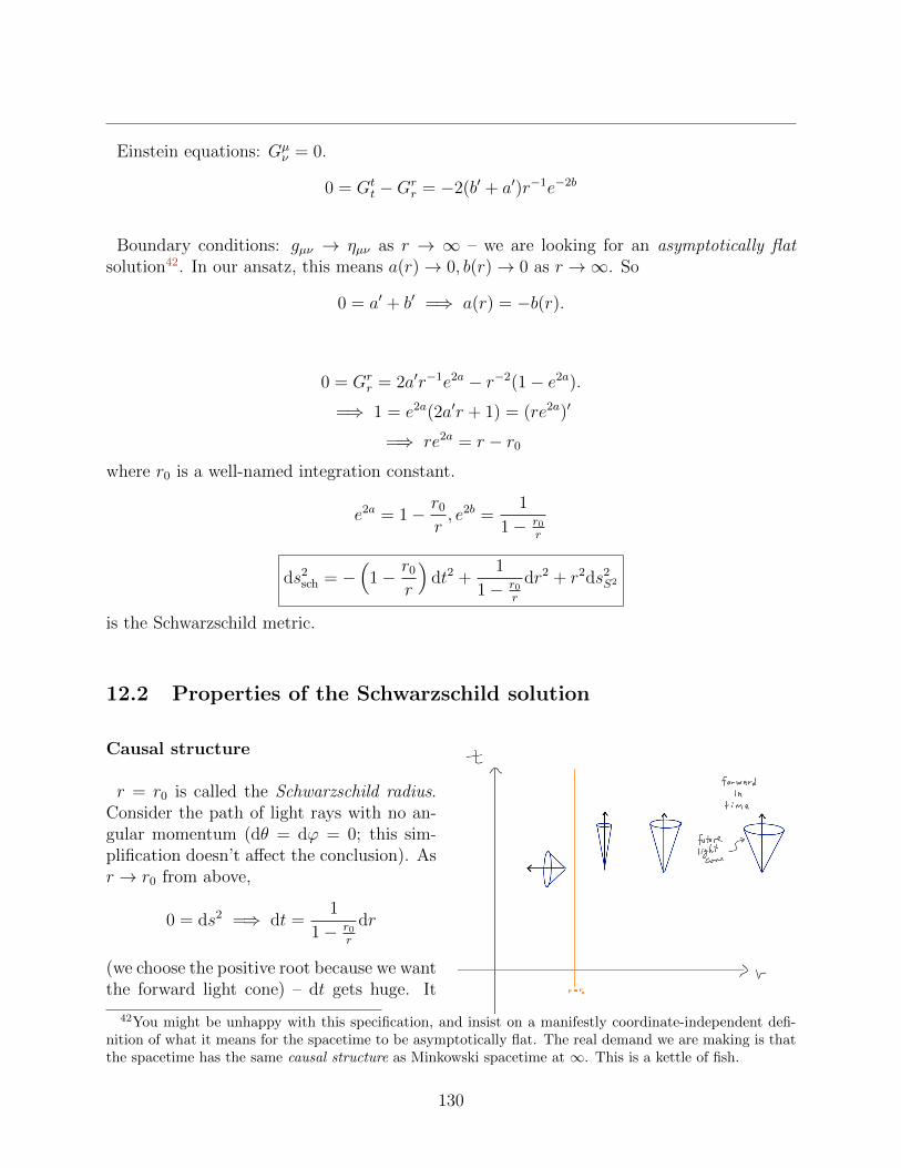
Einstein equations: Gµν = 0.

0 = Gtt −Gr

r = −2(b′ + a′)r−1e−2b

Boundary conditions: gµν → ηµν as r → ∞ – we are looking for an asymptotically flatsolution42. In our ansatz, this means a(r)→ 0, b(r)→ 0 as r →∞. So

0 = a′ + b′ =⇒ a(r) = −b(r).

0 = Grr = 2a′r−1e2a − r−2(1− e2a).

=⇒ 1 = e2a(2a′r + 1) = (re2a)′

=⇒ re2a = r − r0

where r0 is a well-named integration constant.

e2a = 1− r0

r, e2b =

1

1− r0r

ds2sch = −

(1− r0

r

)dt2 +

1

1− r0r

dr2 + r2ds2S2

is the Schwarzschild metric.

12.2 Properties of the Schwarzschild solution

Causal structure

r = r0 is called the Schwarzschild radius.Consider the path of light rays with no an-gular momentum (dθ = dϕ = 0; this sim-plification doesn’t affect the conclusion). Asr → r0 from above,

0 = ds2 =⇒ dt =1

1− r0r

dr

(we choose the positive root because we wantthe forward light cone) – dt gets huge. It

42You might be unhappy with this specification, and insist on a manifestly coordinate-independent defi-nition of what it means for the spacetime to be asymptotically flat. The real demand we are making is thatthe spacetime has the same causal structure as Minkowski spacetime at ∞. This is a kettle of fish.

130

takes longer and longer to move a fixed radial coordinate distance dr. The lightcones closeup; as we pass through r = r0, they flip over: for r < r0, t becomes spacelike and r becomestimelike! Nothing can escape r < r0. Hence the name ‘black hole’.

Plugging in numbers

We have already seen that in the Newtonian limit, gtt = − (1 + 2φ(r)), so if this metricresults from a collection of mass centered at r = 0, we have the Newtonian potential

φ = −GNM

r=⇒ r0 = 2GNM.

So as the object gets heavier, the Schwarzschild radius grows (linearly in D = 3 + 1 dimen-sions).

The sun has Msun ∼ 1057GeV and Rsun ∼ 106km. The Schwarzschild radius for this massis

r0(s) = 2GNMsun ∼ 2(10−38GeV−2)(1057GeV) ∼ 1019GeV−1 ∼ 105cm ∼ 1km.

So the mass density of a solar mass black hole is ρBH ∼ 1018ρsun ∼ 1GeV4. Nuclear densityis ρnuc ∼ 1GeV

1fermi3∼ 10−3GeV4. On the other hand, it’s not clear that “density” is the right

way to think about what’s inside a black hole.

131

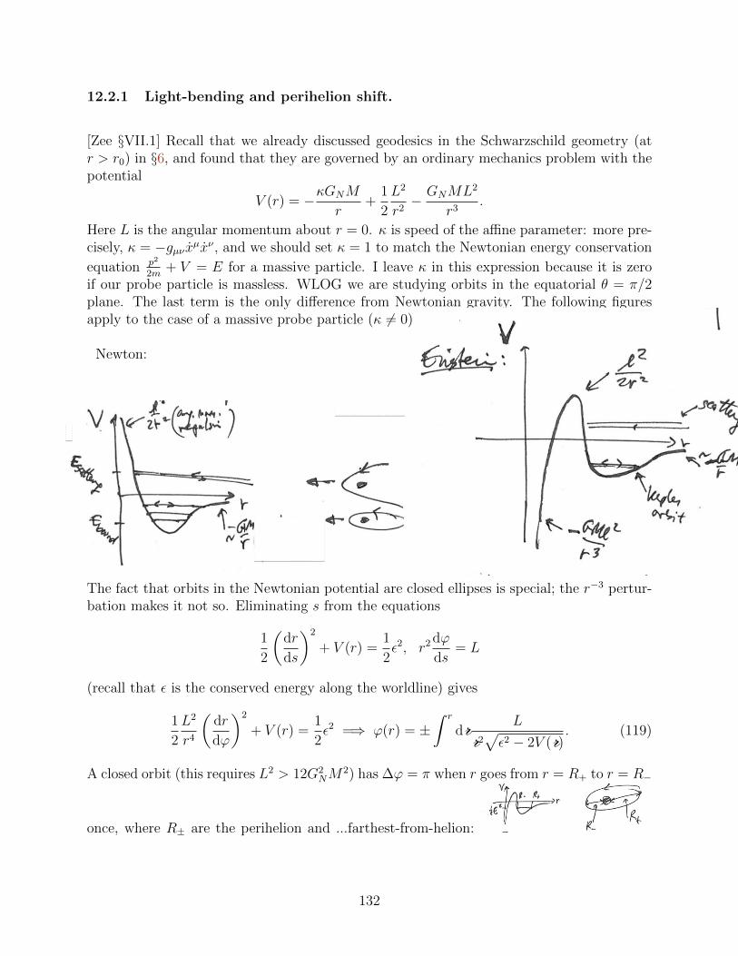
12.2.1 Light-bending and perihelion shift.

[Zee §VII.1] Recall that we already discussed geodesics in the Schwarzschild geometry (atr > r0) in §6, and found that they are governed by an ordinary mechanics problem with thepotential

V (r) = −κGNM

r+

1

2

L2

r2− GNML2

r3.

Here L is the angular momentum about r = 0. κ is speed of the affine parameter: more pre-cisely, κ = −gµν xµxν , and we should set κ = 1 to match the Newtonian energy conservation

equation p2

2m+ V = E for a massive particle. I leave κ in this expression because it is zero

if our probe particle is massless. WLOG we are studying orbits in the equatorial θ = π/2plane. The last term is the only difference from Newtonian gravity. The following figuresapply to the case of a massive probe particle (κ 6= 0).

Newton:

The fact that orbits in the Newtonian potential are closed ellipses is special; the r−3 pertur-bation makes it not so. Eliminating s from the equations

1

2

(dr

ds

)2

+ V (r) =1

2ε2, r2 dϕ

ds= L

(recall that ε is the conserved energy along the worldline) gives

1

2

L2

r4

(dr

dϕ

)2

+ V (r) =1

2ε2 =⇒ ϕ(r) = ±

∫ r

dr L

r2√ε2 − 2V (r)

. (119)

A closed orbit (this requires L2 > 12G2NM

2) has ∆ϕ = π when r goes from r = R+ to r = R−

once, where R± are the perihelion and ...farthest-from-helion:

132

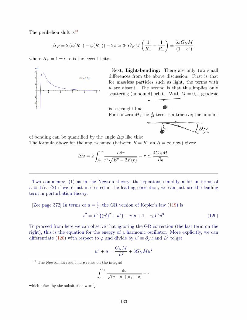
The perihelion shift is43

∆ϕ = 2 (ϕ(R+)− ϕ(R−))− 2π ' 3πGNM

(1

R+

+1

R−

)=

6πGNM

(1− e2),

where R± = 1± e, e is the eccentricity.

Next, Light-bending: There are only two smalldifferences from the above discussion. First is thatfor massless particles such as light, the terms withκ are absent. The second is that this implies onlyscattering (unbound) orbits. With M = 0, a geodesic

is a straight line:For nonzero M , the 1

r3 term is attractive; the amount

of bending can be quantified by the angle ∆ϕ like this:The formula above for the angle-change (between R = R0 an R =∞ now) gives:

∆ϕ = 2

∫ ∞R0

Ldr

r2√E2 − 2V (r)

− π ' 4GNM

R0

.

Two comments: (1) as in the Newton theory, the equations simplify a bit in terms ofu ≡ 1/r. (2) if we’re just interested in the leading correction, we can just use the leadingterm in perturbation theory.

[Zee page 372] In terms of u = 1r, the GR version of Kepler’s law (119) is

ε2 = L2((u′)2 + u2

)− r0u+ 1− r0L

2u3 (120)

To proceed from here we can observe that ignoring the GR correction (the last term on theright), this is the equation for the energy of a harmonic oscillator. More explicitly, we candifferentiate (120) with respect to ϕ and divide by u′ ≡ ∂ϕu and L2 to get

u′′ + u =GNM

L2+ 3GNMu2

43 The Newtonian result here relies on the integral∫ u+

u−

du√(u− u−)(u+ − u)

= π

which arises by the subsitution u = 1r .

133

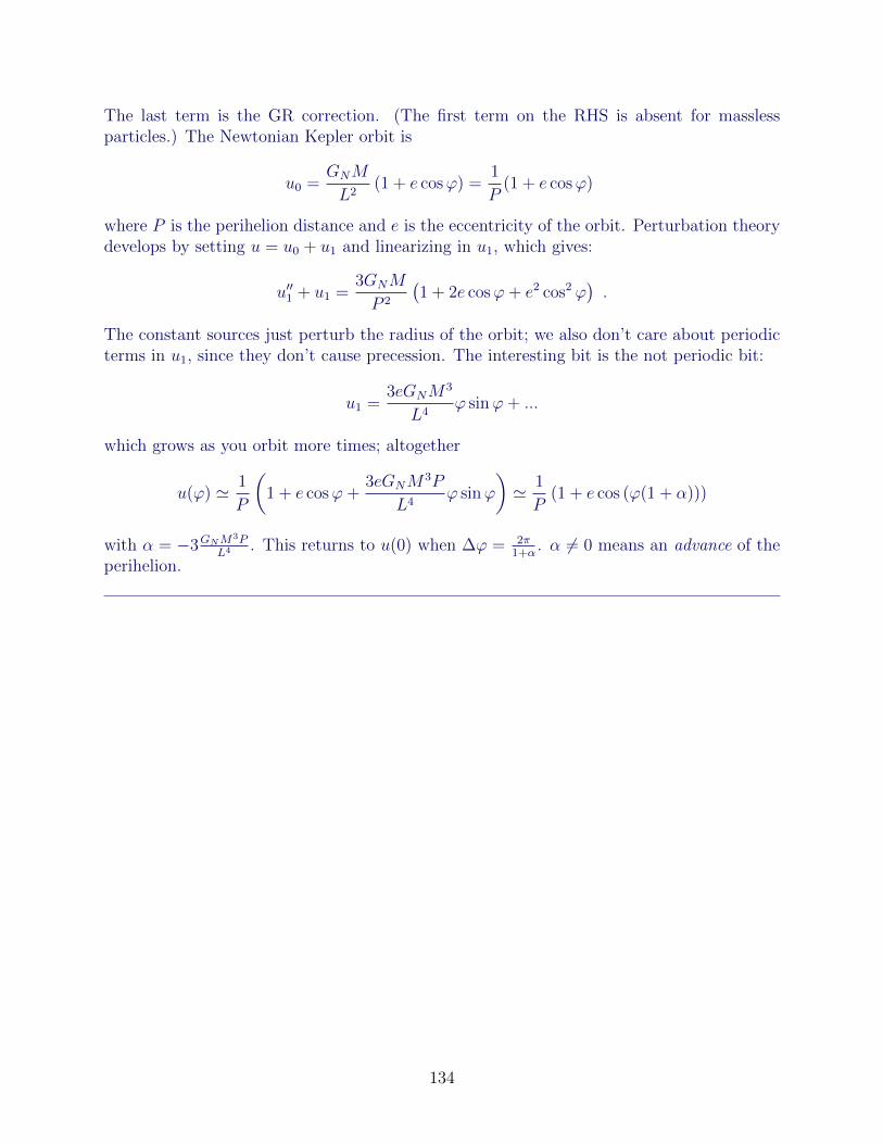
The last term is the GR correction. (The first term on the RHS is absent for masslessparticles.) The Newtonian Kepler orbit is

u0 =GNM

L2(1 + e cosϕ) =

1

P(1 + e cosϕ)

where P is the perihelion distance and e is the eccentricity of the orbit. Perturbation theorydevelops by setting u = u0 + u1 and linearizing in u1, which gives:

u′′1 + u1 =3GNM

P 2

(1 + 2e cosϕ+ e2 cos2 ϕ

).

The constant sources just perturb the radius of the orbit; we also don’t care about periodicterms in u1, since they don’t cause precession. The interesting bit is the not periodic bit:

u1 =3eGNM

3

L4ϕ sinϕ+ ...

which grows as you orbit more times; altogether

u(ϕ) ' 1

P

(1 + e cosϕ+

3eGNM3P

L4ϕ sinϕ

)' 1

P(1 + e cos (ϕ(1 + α)))

with α = −3GNM3P

L4 . This returns to u(0) when ∆ϕ = 2π1+α

. α 6= 0 means an advance of theperihelion.

134

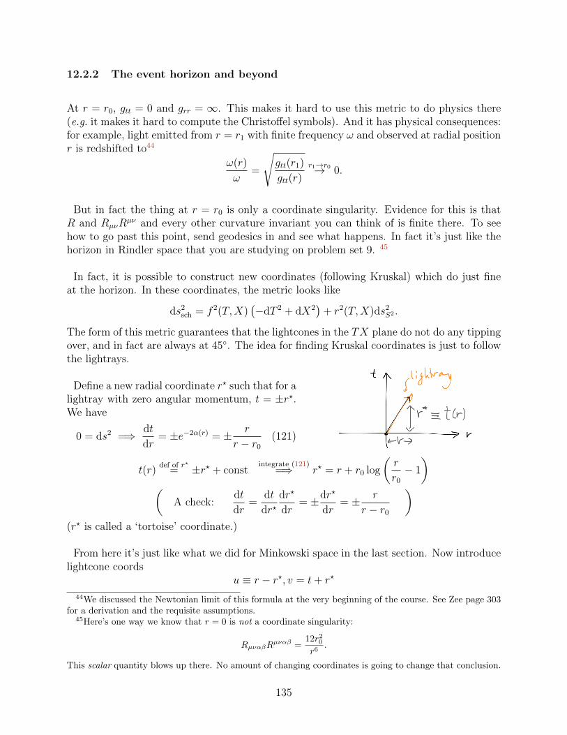
12.2.2 The event horizon and beyond

At r = r0, gtt = 0 and grr = ∞. This makes it hard to use this metric to do physics there(e.g. it makes it hard to compute the Christoffel symbols). And it has physical consequences:for example, light emitted from r = r1 with finite frequency ω and observed at radial positionr is redshifted to44

ω(r)

ω=

√gtt(r1)

gtt(r)

r1→r0→ 0.

But in fact the thing at r = r0 is only a coordinate singularity. Evidence for this is thatR and RµνR

µν and every other curvature invariant you can think of is finite there. To seehow to go past this point, send geodesics in and see what happens. In fact it’s just like thehorizon in Rindler space that you are studying on problem set 9. 45

In fact, it is possible to construct new coordinates (following Kruskal) which do just fineat the horizon. In these coordinates, the metric looks like

ds2sch = f 2(T,X)

(−dT 2 + dX2

)+ r2(T,X)ds2

S2 .

The form of this metric guarantees that the lightcones in the TX plane do not do any tippingover, and in fact are always at 45. The idea for finding Kruskal coordinates is just to followthe lightrays.

Define a new radial coordinate r? such that for alightray with zero angular momentum, t = ±r?.We have

0 = ds2 =⇒ dt

dr= ±e−2α(r) = ± r

r − r0

(121)

t(r)def of r?

= ±r? + constintegrate (121)

=⇒ r? = r + r0 log

(r

r0

− 1

)(

A check:dt

dr=

dt

dr?dr?

dr= ±dr?

dr= ± r

r − r0

)(r? is called a ‘tortoise’ coordinate.)

From here it’s just like what we did for Minkowski space in the last section. Now introducelightcone coords

u ≡ r − r?, v = t+ r?

44We discussed the Newtonian limit of this formula at the very beginning of the course. See Zee page 303for a derivation and the requisite assumptions.

45Here’s one way we know that r = 0 is not a coordinate singularity:

RµναβRµναβ =

12r20r6

.

This scalar quantity blows up there. No amount of changing coordinates is going to change that conclusion.

135

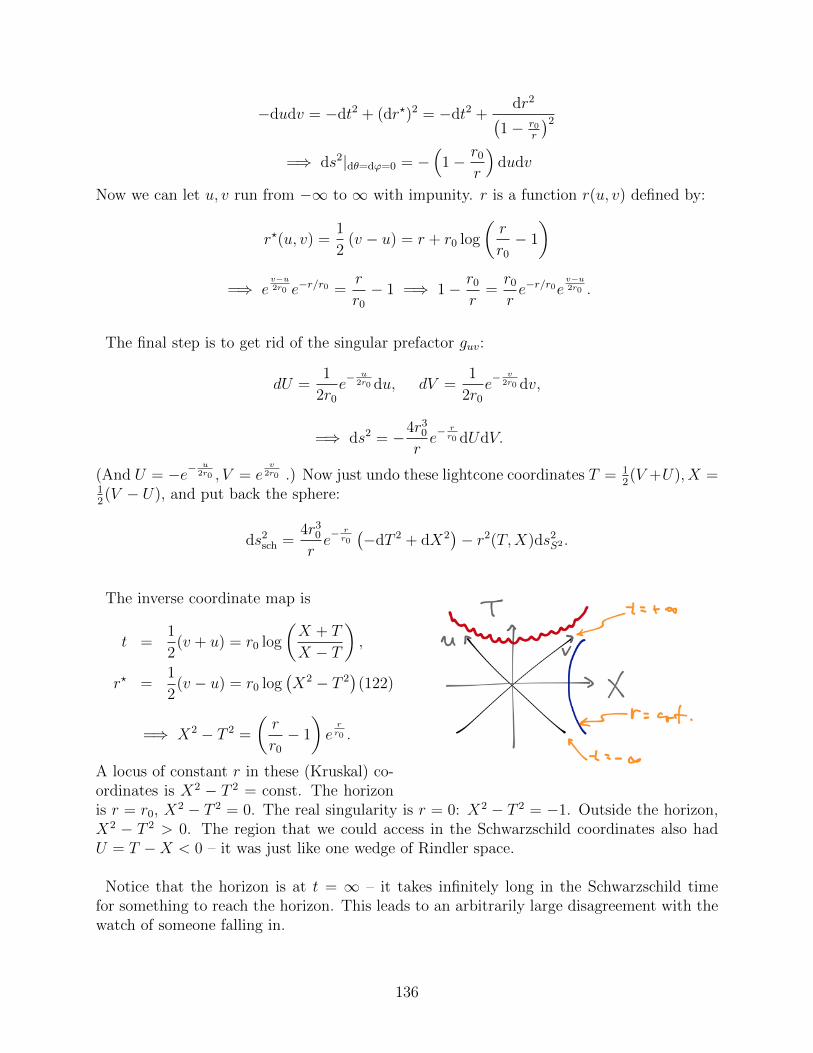
−dudv = −dt2 + (dr?)2 = −dt2 +dr2(

1− r0r

)2

=⇒ ds2|dθ=dϕ=0 = −(

1− r0

r

)dudv

Now we can let u, v run from −∞ to ∞ with impunity. r is a function r(u, v) defined by:

r?(u, v) =1

2(v − u) = r + r0 log

(r

r0

− 1

)=⇒ e

v−u2r0 e−r/r0 =

r

r0

− 1 =⇒ 1− r0

r=r0

re−r/r0e

v−u2r0 .

The final step is to get rid of the singular prefactor guv:

dU =1

2r0

e− u

2r0 du, dV =1

2r0

e− v

2r0 dv,

=⇒ ds2 = −4r30

re− rr0 dUdV.

(And U = −e−u

2r0 , V = ev

2r0 .) Now just undo these lightcone coordinates T = 12(V +U), X =

12(V − U), and put back the sphere:

ds2sch =

4r30

re− rr0

(−dT 2 + dX2

)− r2(T,X)ds2

S2 .

The inverse coordinate map is

t =1

2(v + u) = r0 log

(X + T

X − T

),

r? =1

2(v − u) = r0 log

(X2 − T 2

)(122)

=⇒ X2 − T 2 =

(r

r0

− 1

)err0 .

A locus of constant r in these (Kruskal) co-ordinates is X2 − T 2 = const. The horizonis r = r0, X2 − T 2 = 0. The real singularity is r = 0: X2 − T 2 = −1. Outside the horizon,X2 − T 2 > 0. The region that we could access in the Schwarzschild coordinates also hadU = T −X < 0 – it was just like one wedge of Rindler space.

Notice that the horizon is at t = ∞ – it takes infinitely long in the Schwarzschild timefor something to reach the horizon. This leads to an arbitrarily large disagreement with thewatch of someone falling in.

136

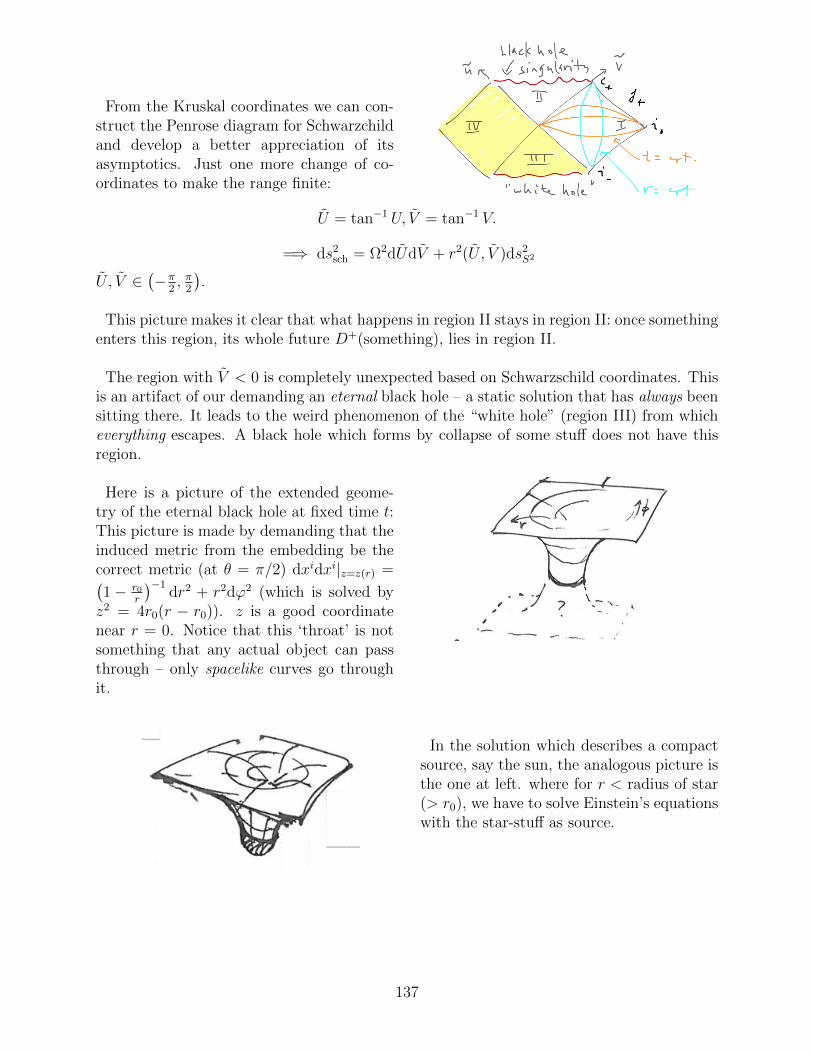
From the Kruskal coordinates we can con-struct the Penrose diagram for Schwarzchildand develop a better appreciation of itsasymptotics. Just one more change of co-ordinates to make the range finite:

U = tan−1 U, V = tan−1 V.

=⇒ ds2sch = Ω2dUdV + r2(U , V )ds2

S2

U , V ∈(−π

2, π

2

).

This picture makes it clear that what happens in region II stays in region II: once somethingenters this region, its whole future D+(something), lies in region II.

The region with V < 0 is completely unexpected based on Schwarzschild coordinates. Thisis an artifact of our demanding an eternal black hole – a static solution that has always beensitting there. It leads to the weird phenomenon of the “white hole” (region III) from whicheverything escapes. A black hole which forms by collapse of some stuff does not have thisregion.

Here is a picture of the extended geome-try of the eternal black hole at fixed time t:This picture is made by demanding that theinduced metric from the embedding be thecorrect metric (at θ = π/2) dxidxi|z=z(r) =(1− r0

r

)−1dr2 + r2dϕ2 (which is solved by

z2 = 4r0(r − r0)). z is a good coordinatenear r = 0. Notice that this ‘throat’ is notsomething that any actual object can passthrough – only spacelike curves go throughit.

In the solution which describes a compactsource, say the sun, the analogous picture isthe one at left. where for r < radius of star(> r0), we have to solve Einstein’s equationswith the star-stuff as source.

137

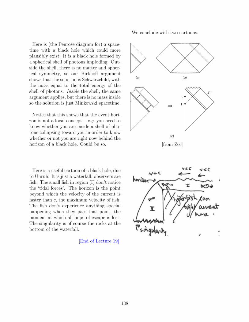
We conclude with two cartoons.

[from Zee]

Here is (the Penrose diagram for) a space-time with a black hole which could moreplausibly exist: It is a black hole formed bya spherical shell of photons imploding. Out-side the shell, there is no matter and spher-ical symmetry, so our Birkhoff argumentshows that the solution is Schwarzchild, withthe mass equal to the total energy of theshell of photons. Inside the shell, the sameargument applies, but there is no mass insideso the solution is just Minkowski spacetime.

Notice that this shows that the event hori-zon is not a local concept – e.g. you need toknow whether you are inside a shell of pho-tons collapsing toward you in order to knowwhether or not you are right now behind thehorizon of a black hole. Could be so.

Here is a useful cartoon of a black hole, dueto Unruh: It is just a waterfall; observers arefish. The small fish in region (I) don’t noticethe ‘tidal forces’. The horizon is the pointbeyond which the velocity of the current isfaster than c, the maximum velocity of fish.The fish don’t experience anything specialhappening when they pass that point, themoment at which all hope of escape is lost.The singularity is of course the rocks at thebottom of the waterfall.

[End of Lecture 19]

138