physics 1050 lab manual spring 2010

Department of Physics & Astronomy

PHYSICS 1050 LAB MANUAL

SPRING 2010

i

Table of Contents

Lab Reports and Marks .................................................................................................. i

Sample Lab Manual ....................................................................................................... iii

Sample Lab Report ........................................................................................................ v

Statistics………………………………………………………………………………………...1

Free Fall ....................................................................................................................... 13

Projectile Motion ......................................................................................................... 16

Vectors, Forces, and Equilibrium ............................................................................. 20

Mechanics of the Human Arm ................................................................................... 27

Angular Acceleration of a Disk ................................................................................. 32

Principles of Mechanics ............................................................................................ 36

Conservation of Momentum ....................................................................................... 39

Speed of Sound ........................................................................................................... 42

Nuclear Half Life .......................................................................................................... 48

i

LAB REPORTS AND MARKS

This section includes an outline for your lab reports and a sample lab report based on an experiment called “Conservation of Energy on an Inclined Plane” (also included). Since your marks for the lab are derived from your written reports it is important to understand what is expected as a report. Read the sample experimental outline “Conservation of Energy on an Inclined Plane” first, then the lab report outline, and conclude by reading the sample report. LAB REPORT OUTLINE: Lab reports must have the following format: 1. Title Page: Includes the title of experiment, the date the experiment was

performed, your name, your partner's name(s), and lab section. 2. Results: List data in tables whenever possible. Each table must have a title

and carry units for each column. Show one sample calculation for each step in the analysis, carrying the units through the calculations.

3. Graphs: When asked to plot a graph be sure to label each axis including

units. Each graph must have a descriptive title placed above the graph (note: Y vs X is not a descriptive title).

4. Analysis: Complete all steps and questions in the analysis section of the

experimental outline. 5. Discussion: A brief paragraph outlining the important facets and details of your

experimental results. 6. Conclusion: A final sentence(s) stating the outcome(s) of the experiment written

in the context of the objective of the experiment. If you glance through a scientific journal you will observe that the outline listed above is a simplified version of most journal formats. Items such as abstracts, introduction, and procedure have been omitted. The difference between a “good” lab write-up and a poor one is often attention to detail. As you write your report you must assume that the person who will read it knows little about your experiment. You are presenting a case upon which you will base your conclusion. Guide the reader through the report by clearly labeling tables and graphs with descriptive titles, succinctly presenting your discussion of the experiment and results, and unambiguously stating your conclusion(s).

ii

Marking scheme: Each student is required to submit one lab report for each

experiment unless directed otherwise. Students complete some experiments in Physics 1050 in groups and others on an individual basis. When experiments are done in groups one lab report for the group is sufficient, although individual group members may submit their own report if they prefer. When group reports are marked each member of the group receives the same mark.

Lab reports are due one week after each experiment is completed.

Lab reports will generally be marked out of 10 (longer labs may be marked out of 15).

Your final lab mark is calculated as:

Total Marks Received / Total Marks Possible Note: If you are repeating the course and wish to transfer your previous lab mark (must be at least 50%) for credit in the current course you may do so by applying in writing to the Physics Department chair. Include in your submission your ID number and the year and semester in which you previously took the course.

iii

CONSERVATION OF ENERGY ON AN INCLINED PLANE OBJECTIVE: The objective of this experiment is to investigate the principle of

conservation of energy using an inclined plane. APPARATUS: Air Track

Sonar System Carpenter‟s Level Meter Sticks

BACKGROUND: The near frictionless surface of an air track represents a close

approximation to something called an isolated system. Such a system would be expected to demonstrate the principle of conservation of mechanical energy.

By definition an isolated system does not exchange mass or energy with its surroundings. Any mechanical energy put into the system will remain there and we should be able to account for it as either kinetic or potential energy. If the principle of conservation of mechanical energy is correct then the total energy in the system should remain constant.

Tipping the air track at an angle creates what physicists call an inclined plane. In the absence of friction an object placed on an inclined plane will begin to move in the downhill direction.

Energy is introduced into the inclined plane system by placing the glider at the top of the incline. Until released all the energy in the system is in the form of potential energy. Once moving some of the potential energy is transformed into kinetic energy. As the glider progresses down the incline the potential energy continues to decrease while the kinetic energy increases. At any instant in time,

iv

however, the sum of the two should be constant and equal the initial amount of potential energy in the system.

PROCEDURE: Set the air tack at a slight angle to the horizontal (about 2 degrees).

Place the glider at the high end of the air track and allow it slide to the low end. Track the position of the glider during its travel using the sonar equipment. Save your data on a disk. Be sure to record the mass of the glider and measure the angle of incline with two meter sticks and the carpenter‟s level.

ANALYSIS: Construct a data table like the one below and make the appropriate

calculations.

Time (sec)

Position of Glider (cm)

Velocity of Glider (cm/sec)

Kinetic Energy of Glider (J)

Potential Energy of Glider (J)

Total Energy (J)

From your calculations plot on a single graph the potential, kinetic and total energies as a function of time.

Include in your lab write-up the answers to the following questions:

1) How accurately were you able to measure the angle of

incline? 2) What impact(s) might an error in the measurement of the

angle of incline have on the results of the experiment?

v

CONSERVATION OF ENERGY ON AN INCLINED PLANE

Larry Brown Curly Jones Moe Smith

Thursday, Jan. 8, 2004 Lab Section #2

vi

Table #1. Inclined Plane Data Table Mass of glider (gm) - 220 Delta T (sec) - 0.0500 Angle of incline (deg) - 2.70

Time (sec)

Position (cm)

Velocity (m/sec)

Potential Energy (J)

Kinetic

Energy (J)

Total

Energy (J) 1.1 198.43 0.316 0.2015 0.0110 0.213

1.2 196.85 0.330 0.1999 0.0120 0.212

1.3 195.20 0.428 0.1982 0.0202 0.218

1.4 193.06 0.402 0.1961 0.0178 0.214

1.5 191.05 0.352 0.1940 0.0136 0.208

1.6 189.29 0.508 0.1922 0.0284 0.221

1.7 186.75 0.450 0.1897 0.0223 0.212

1.8 184.50 0.442 0.1874 0.0215 0.209

1.9 182.29 0.518 0.1851 0.0295 0.215

2.0 179.70 0.590 0.1825 0.0383 0.221

2.1 176.75 0.568 0.1795 0.0355 0.215

2.2 173.91 0.598 0.1766 0.0393 0.216

2.3 170.92 0.632 0.1736 0.0439 0.218

2.4 167.76 0.652 0.1704 0.0468 0.217

2.5 164.50 0.644 0.1671 0.0456 0.213

2.6 161.28 0.690 0.1638 0.0524 0.216

2.7 157.83 0.772 0.1603 0.0656 0.226

2.8 153.97 0.696 0.1564 0.0533 0.210

2.9 150.49 0.812 0.1528 0.0725 0.225

3 146.43 0.778 0.1487 0.0666 0.215

3.1 142.54 0.806 0.1448 0.0715 0.216

3.2 138.51 0.826 0.1407 0.0751 0.216

3.3 134.38 0.826 0.1365 0.0751 0.212

3.4 130.25 0.896 0.1323 0.0883 0.221

3.5 125.77 0.880 0.1277 0.0852 0.213

4.0 121.37 0.912 0.1233 0.0915 0.215

4.1 116.81 0.932 0.1186 0.0955 0.214

vii

Sample Calculations Notes: 1.) The position data column represents the distance from the sonar

unit to the glider. 2.) The frequency of the sonar unit was 20 Hz. which translates into a

delta T of .0500 seconds. Velocity Calculation

Velocity is defined as,

ΔPosition

Δtime

Each entry in the velocity was calculated as, t

PP NN 1

Sample calculation:

sec/6.310500.0

85.19643.198cm

Potential Energy Calculation Potential energy is defined as, PE = (mass) (acceleration of gravity) (height) Given that the data can be thought of as the hypotenuse of a right-hand triangle, the height can be calculated as,

h = (data) sin ( )

PE = (m) (g) (data) sin ( )

Sample calculation: (.220) (9.8) (1.9843) (sin (2.7)) = .2015 (J) Kinetic Energy Calculation Kinetic energy is defined as KE = ½ (mass) (velocity)2 Sample calculation: (.5) (.220) (.316)2 = .0110 (J) Total energy is the sum of the potential and kinetic energies.

viii

Figure 1

0

0.05

0.1

0.15

0.2

0.25

En

erg

y (

Jo

ule

s)

1 1.5 2 2.5 3 3.5 4 Time (seconds)

Total Energy Kinetic Energy Potential Energy

Conservation of Energyon an Inclined Plane

ix

Discussion: It can be seen from figure 1 energy was conserved as the glider descended the air track. We checked to see if air resistance was a problem. We found that the velocity of the glider (see figure 2) was linear and therefore air resistance did not affect our results. The fact that the velocity was linear also tells us that acceleration on the air track is constant.

Figure 2 Measurement of the angle of the air track is a concern. If the angle is improperly measured the potential energy calculations will be inaccurate. The result could be an

0.3

0.4

0.5

0.6

0.7

0.8

0.9

1

Ve

loc

ity

(c

m/s

)

1.1 1.3 1.5 1.7 1.9 2.1 2.3 2.5 2.7 2.9 3.1 3.3 3.5 4.1

Time (seconds)

Velocity on an Inclined Plane

x

apparent increase or decrease in the total energy when in reality energy is conserved. We measured the angle several times and used the average value as the actual angle of incline for the air track. Conclusion: Energy was conserved on the inclined plane. Responses to questions:

1.) Each member of the group measured the angle of incline several times. We found the accuracy of the measurement to be about one half of one degree. The limiting factor in measuring the angle is the carpenter’s level.

2.) The experimental calculations are quite sensitive to the value used for the angle of incline. This is because this angle is used to calculate the potential energy. Using the same data, and varying the angle over a range of 1.5 degrees, we were able to get a variety of results. Over this range of angles we could show a loss of energy or a gain of energy.

1

STATISTICS

OBJECTIVE: The objective of this exercise is to familiarize the student with the

use of Gaussian distributions, linear regression, and Chauvenet‟s criterion as they relate to data analysis for experiments in physics 1000.

BACKGROUND: Statistical analysis plays a very important role in experimental

work. In this exercise we are concerned with the connotations of terms such as average, standard deviation, and normal distribution, as these terms have particular meanings when associated with experimental work. In addition, we will develop quantitative tools for judging the validity of data.

Throughout the semester we will associate the term average or mean with the "best estimate of the actual value". Standard deviation will represent the "average value of uncertainty in the average" or probable error, and a normal distribution will be viewed as a probability distribution. We will use techniques such as linear regression and Chauvenet's criterion to provide methods for assessing the validity of data gathered during experiments.

The following sections are brief overviews of the important points as they relate to statistical analysis.

Gaussian Distributions

The Gaussian curve, named after Karl Friedrich Gauss, was devised in 1795. Gauss found that his experimental data would not repeat itself exactly from trial to trial during experiments. After plotting the results of a particular experiment he developed his now famous curve.

Gaussian distributions are also called normal distributions or bell curves. The term bell curve obviously arose from the symmetrical curved shape of the Gaussian distribution while the name normal distribution is related to one of the mathematical requirements of a Gaussian distribution; that it be normalized. In practice all three terms are used interchangeably and refer to a symmetrical distribution of values caused by random error. There are other types of distributions used in statistical analysis which differ from

2

Gaussian distributions (e.g. Poisson distributions or binomial distributions). We will confine our interest solely to Gaussian distributions as they are applicable to the type of experimental work we will do this semester.

Any time measurements are made they are subject to some degree of uncertainty. This is known as experimental error. When the error is small and random (as opposed to systematic) then it can be shown that the repeated measurements of the same quantity will cluster around the actual or true value of the measurement. Further, it can be shown that distribution of values around the true value will be symmetrical and have a curved shaped (the bell curve).

The “actual”, “best”, or “true” value of a set of measurements is, as you probably already know, called the average or mean. It can be shown mathematically that this is the case, however, we will be content at this time to simply except the fact.

If we call any measurement we have made, x, then the average of a set of x‟s can be calculated as:

The width of the distribution curve about the average is also important. If it is narrow then most values are close to the average.

Average = X =

N

i=1

xi

N

3

If it is wide then the values are not as close to the average. A narrow distribution indicates higher precision (lower error) than a wide distribution.

The width of a Gaussian distribution is denoted by its standard deviation. Standard deviation represents the average difference of a given measurement from the value of the mean.

N

i

ixxN 1

22

1

1

If you look closely at the equation for calculating standard deviation you can see that you are taking the average of the differences between the data points in the set and the average of the set. If the standard deviation is numerically large then the distribution is wide. If it is numerically small then the distribution is narrow. Naturally then the standard deviation is a measure of experimental error.

It can be shown that the standard deviation of a data set is equivalent to calculating the probable error in the value of the average for the data set.

4

A Gaussian distribution (shape of the curve) is expressed mathematically as,

where N is the number of times a given measurement is

observed Nmax = the measurement which is observed most often x = average value of all measurements σ = standard deviation, defined by

where n = total number of measurements

xi = results of the ith measurement.

There is an interesting and useful relationship between a Gaussian distribution and its standard deviation.

In any Gaussian distribution 68% of the total area under the curve falls in the region from x - σ to x + σ. 95% of the total area falls

between x - 2σ and x + 2σ. This tells us that if an experiment is

done to measure some quantity, although the result is not duplicated exactly each time, there will be a definite pattern in the results. First there will be a tendency toward some central value (x ). Second, 68% of all values will fall within one standard

5

deviation of x and 95% of all values will fall between x - 2σ and x + 2σ. Thus, it is reasonable to associate σ with the uncertainty in a given set of measurements and to view the Gaussian distribution as a probability curve.

For experiments done in the lab, use the following definition of standard deviation σx. (On your calculator this function is usually denoted as σn-1.)

An example: Consider the measurement of a steel rod using a

micrometer (accurate to .001 cm). The results are listed below.

The standard deviation is:

Therefore, the length of the rod is: 10.351 ± .002 cm.

σ2x =

1n-1

n

i=1

( x - xi)2.

6

Chauvenet's Criterion

Another important consideration in experimental work is judging the validity of data. Inevitably when doing experiments data is generated which upon inspection seems to be incorrect. If mistakes have been made during the experiment then it is easy to discard the data, however, if the experimental process is found to be valid then one must treat the data very carefully. More than one Nobel prize in physics has been awarded because someone would not throw away what was considered to be “bad data” at the time.

We will use Gaussian distributions as probability distributions in assessing the validity of data. As an example consider the following set of measurements of some quantity:

3.9, 3.5, 4.0, 4.0, 3.4, 4.1, 1.9

At first glance the value 1.9 appears to be incorrect when compared to the other values. Can the value of 1.9 simply be disregarded because it differs from the rest? If no evidence of malfunction in equipment and/or mistake in procedure can be found then one must provide a justification for the rejection of data. One school of thought suggests that rejection of data is never justified. A somewhat more practical solution is to assess the probability that the suspect data is correct (Chauvenet's criterion).

In order to use Chauvenet's criterion the student must be comfortable with the concepts of average and standard deviation and have realized that a Gaussian distribution is in fact a probability curve. The first step in assessing the data is to calculate the average and standard deviation of the data (including the suspect value of 1.9).

x = 3.5 σx = .77

Knowing the magnitude of the standard deviation makes it possible to calculate the difference between the suspect value (xsus) and the average value in terms of the number of standard deviations (#Sd's).

Recall that in a Gaussian distribution 68% of all measurements fall within 1 standard deviation of the mean, 95% within 2 standard deviations of the mean and so on. Another way of saying this is

7

that 32% of all values will be outside one standard deviation from the average value and only 5% of all values will be farther away from the average than two standard deviations. In other words the farther away a value is from the average value, the less probable it is to be present in the data set.

It is possible to calculate the exact probability if one has a table or a computer to provide the values. Table 1 (page 9) lists the area under a Gaussian curve as a function of the width measured in standard deviations. Let‟s call the probability of being part of this area, Prob(inside).

Since all of the area under the curve represents 100% of the possibilities then the probability of being outside a certain portion of the curve ( Prob(outside)) would simply be 1 - Prob(inside). For our example we get 96.43% or .9643 from Table 1, meaning that 96.43% of all our data should be within 2.1 standard deviations of the average.

Prob (outside 2.1σx) = 1 - Prob (inside 2.1σx)

= 1 - .9643 = .0357 ≈ .036.

Therefore only 3.6% of all measurements would be farther away from the average.

Now the important part. In experimental work there is no such thing as part of a measurement. You either make a measurement or you don‟t make a measurement. How many measurements do you need to make in order that one measurement represents 3.6% of the total number of measurements?

The number .036 suggests that if there were 28 (1/.036) measurements we should expect to see a value of 1.9, however, in a set of 7 measurements we would expect only .25 of a measurement (.036 x 7) to have a value around 1.9. We must therefore decide whether .25 is sufficient to indicate that 1.9 is an "improbable" value for this set of measurements. Chauvenet's criterion sets the value of “improbability" at .5. In other words if the probability of a value falling outside a given number of standard deviations (Prob (outside)) multiplied by the total number of measurements is less than .5 then the data may be rejected.

The process for using Chauvenet‟s criterion is summarized as:

1) Calculate x , σx using all the data.

2) Calculate P(outside).

8

P(outside) = 1 - P(inside).

P(inside) comes from a table or calculation.

3) Multiply P(outside) by the number of data points in the set. Compare this number with Chauvenet's Criterion.

4) If C.C. .5 the data point(s) is good. If C.C. < .5 reject the data point(s).

NOTE: If data is rejected a new x , σx must be calculated based on

the remaining data.

An Alternate Approach......

Suppose you have 500 data points of which 35 are suspicious. Do you need to use Chauvenet's Criterion on each point? No, Chauvenet's Criterion is based on the number of data points in the set. Begin by calculating P(outside) from

P(outside)

= .5

number of data points

and then work backwards to calculate the bounds of σ for valid data.

9

TABLE 1. Percentage Probability (Area Under a Gaussian Curve)

10

LINEAR REGRESSION

Linear regression or least linear squares fitting provides a method by which the "best" straight line fit for a set of data may be calculated. Linear regression does not determine if the relationships in a data set are linear. That must be established by some other means (usually from theory). For example the speed of an object undergoing constant acceleration will change linearly with respect to time. A plot of speed vs. time would therefore be a straight line. Linear regression could be used to determine the slope and intercept of the plot. The fact that the plot is linear is a consequence of the physics of the situation, not the use of linear regression. If the plot where a curve rather than linear it would be meaningless to find a slope and intercept using linear regression.

If we wish to fit a straight line through a set of data in which x is the independent variable and y the dependent variable the following must be true:

· each y value must be governed by a Gaussian distribution with

standard deviation of σy. · the uncertainty in x must be small. · the uncertainties in y must be uniform. · the relationship between x and y must be linear, ie. y = mx + b.

Deriving the equations for linear regression is beyond the scope of Physics 1000. They are developed by applying probability techniques to Gaussian distributions. The results of the derivation, called the normal equations, allow the calculation of the best fit slope and the intercept of the plot.

where

You will use these equations in part II of this exercise.

INTERCEPT = ( x

2

i)( y

i) - ( x

i)( x

iy

i)

Δ

SLOPE = N( x

iy

i) - ( x

i)( y

i)

Δ

Δ = N( x2

i) - ( x

i)2

Physics 1050 Free Fall 11/4

11

PROCEDURE: PART I

This exercise requires two sets of data, which are the results of measurement. Each set must be measured or estimated to the indicated tolerance.

Set #1. The height of each student in physics 1000

(to the nearest cm).

Set #2. The diameter of the metal plate located at the front of the lab (to the nearest mm.).

In each case you will be provided with additional data from previous classes.

ANALYSIS: PART I

1. For each set of data calculate the average and standard deviation. Plot a distribution (histogram) of the number of repetitions of a value vs the range of values. Does it resemble a normal distribution?

2. Use Chauvenet's criterion to determine the "validity" of the

extreme points in the distributions.

3. Answer the following questions:

a. How is the meaning of "average" different for these two sets of data?

b. Do you see anything "interesting" in the distribution plot for

set #1?

c. Locate the definitions of random error and systematic error (use the web). Describe the effects of these two types of errors on a Gaussian distribution.

d. When you apply Chauvenet's Criterion to set #1 are you

assessing the "validity" of the extreme points in the distribution (think about your answer to question #1)?


12

PROCEDURE: PART II - Linear Regression

The data set below represents the position of a moving object with respect to a fixed point. Beneath each position measurement is the corresponding time of the measurement. This relationship is known to be linear (y=mx+b).

Position (M) 6.50 10.70 19.9 21.3 26.9 32.7 38.2 44.1 49.5 Time (Sec) 0.00 1.00 2.00 3.00 4.00 5.00 6.00 7.00 8.00

Using a spreadsheet program, plot the data (position vs time) using a scatter plot, making sure to NOT join the points. Print this plot, and draw on your best estimation of the best-fit line using a ruler and pen. Determine the slope and intercept of this line, and clearly label them in your report as the estimated slope and intercept. Now using the equations contained in the section on linear regression, calculate (show your work) the slope and intercept of the actual best-fit line.

ANALYSIS: PART II

Compare your estimated slope and intercept with those calculated by linear regression and comment.

What are the physical interpretations of slope and intercept in this

case?


13

FREE FALL

OBJECTIVES: The objectives of this experiment are to show that a freely falling

body has constant acceleration, g, and to determine a value for g. BACKGROUND: The term free fall implies a one dimensional motion for which the

motivating force is solely that of gravity. An object falling freely under the influence of gravity in vacuum has an acceleration that is constant, therefore, as the object falls its velocity increases at a constant rate. Any object that moves in a straight line, with equal changes in velocity in equal intervals of time, is said to be moving with uniform, or constant, acceleration.

It should be noted that the terms velocity and speed are not exactly interchangeable. Velocity is a vector, meaning that values for both magnitude and direction are required to fully describe the motion. Speed is by definition the magnitude of the velocity vector. For this experiment we will use the term velocity since the object will experience changes in both speed and direction.

From an experimental point of view the easiest way to determine if the acceleration of an object is constant is to plot its velocity as a function of time. If the plot is linear then the equation which governs the plot is velocity = (acceleration)(time) + initial velocity (recall the equation of a straight line y = mx + b). The slope of the plot is the value of the acceleration while the intercept represents the velocity of the object when the experiment began.

The definition for velocity is,

where Δ means "change in". Equation 1 defines "average velocity over an interval of time". A useful point to remember in situations where the acceleration is constant is that the average velocity over some interval of time is equal to the instantaneous velocity at the mid point( in time) of that interval.

In this experiment we toss a large rubber ball vertically into the air and track its position with a sonar system. The ball rises about two metres and then falls. The speeds associated with these displacements are low enough that air resistance should not be a

Velocity = Displacement

ΔTime(1)


14

significant factor.

Regardless of the fact that the ball first travels upward and then downward the only force acting on the ball after it is tossed is the force of gravity. If the acceleration of the ball is constant then we should see a linear plot of velocity versus time despite the change in direction.

The motion of the ball is tracked by a sonar system that can accurately measure the location of the ball by measuring the time of flight of an ultra sonic sound pulse reflected off the ball. Since the sound pulses are sent at regular intervals of time, Δ t is a constant.

PROCEDURE:

The sonar apparatus will be set-up at the front of the lab. Practice tossing the ball vertically upward such that it rises and falls in a straight line above the sonar device. When you are ready, start the DataStudio program and proceed as follows:

1. Click the “Setup” button, and ensure that the motion sensor

is displayed. If not, click “Add Sensor” and find the motion sensor in the list.

2. Click the “Start” button to begin collecting data. You should

hear a ticking sound while the sonar system is collecting data.

3. Toss the ball into the air, allowing it to rise and fall, catching

it before it hits the sonar system (keep your arms to the side so as not to interfere with the sonar beam). Repeat this step several times to get many trials in your data file.

4. Once you are satisfied with the data use the "Export Data"

entry in the “File” menu to save your data to a suitable medium.

Transfer your data into a spreadsheet, plot all the data, and select a portion of the data which corresponds to the flight of the ball. The portion you use should appear as a smooth parabola, with few erroneous points. Save the selected time and positions for your data table.


15

ANALYSIS: We wish to construct a graph of velocity vs. time. The first step is to construct a data table like the one below:

Time

Position

Velocity

Acceleration

0

Y1

(Y2-Y1)/ΔT = V1

(V2-V1)/ΔT = A1

T1

Y2

(Y3-Y2)/ΔT = V2

(V3-V2)/ΔT = A2

T2

Y3

(Y4-Y3)/ΔT = V3

(V4-V3)/ΔT = A3

T3

Y4

(Y5-Y4)/ΔT = V4

.....Tn

.....Yn

The position and elapse time columns in this data table are the data you selected for the flight of the ball. Reset the time to start at zero. Calculate the velocity as indicated above by calculating the displacement of the ball as the difference in two successive positions of the ball and dividing by the corresponding change in time. The change in time, ΔT, will be constant in this experiment. Plot the velocities against elapsed time and determine the acceleration due to gravity from the slope of the graph (use linear regression). Compare your experimental value for g with the accepted value and compute the percentage difference in your result.

Answer the following questions:

1. Without repeating the experiment, how would you determine

if air resistance is a problem in this experiment?

2. Why are the acceleration values in your data tables not constant?

3. From your plot, can you determine the value of the initial

velocity (Vo ) in this experiment?

Physics 1050 Projectile Motion 16/4

16

PROJECTILE MOTION

OBJECTIVES: The objectives of this experiment are to show that motion in two

dimensions can be treated independently in each dimension and to determine a value for "g", the acceleration due to gravity.

BACKGROUND: Projectile motion, or trajectory motion as it is sometimes called,

refers to the two-dimensional motion of an object projected into the air at an angle (e.g., throwing a baseball or basketball). Analysis of this motion is based on the premise that the vertical and horizontal motions are independent of each other. In order to verify this premise, the trajectory of a steel ball will be analyzed in both the vertical (y) and the horizontal (x) directions. By way of illustration we consider the following example (that is different from the experiment that is actually performed).

A ball is thrown into the air (Fig. 1, point A) having velocity in both the horizontal and vertical directions. At the exact moment it reaches its maximum height (point B) and begins to fall earthward, an identical ball is dropped from the same height (point C).

Figure 1

If the horizontal motion is actually independent of the vertical motion, the balls will strike the ground at the same instant. One expects this to be the case since the only force acting on the balls is gravity (neglecting air resistance) and as a result, Newton's second law predicts that the horizontal motion of ball 1 will remain at its initial constant velocity while both balls will accelerate downward with acceleration g.


17

A strobe photograph of the falling balls would therefore reveal the following.

Figure 2 PROCEDURE: All necessary equipment is assembled in the dark room. You will be

instructed in its operation and will obtain a digital photograph of a projectile. Be sure to record the flash rate (flashes/minute) from the dial of the strobe light.

1. Note the file name of your picture.

2. Download your file from the camera to one of the lab

computers.

3. Using a graphics program locate the pixel positions of the images of the ball in your picture.

4. Subtract the coordinates of the first image of the ball bearing as

it leaves the tube from all your data points (including the first one). The coordinates of the first image of the ball bearing will therefore be 0,0.


18

5. Measure a distance of 10 centimetres on the meter stick in terms of pixels to obtain a scaling factor for your data.

6. Repeat step 5 several times on different sections of the meter

stick.

7. Calculate an overall scale factor by taking the average of measurements. Express your scale factor in units of pixels per cm.

Construct the following table.

Horizontal Coordinate

(pixels)

Vertical

Coordinate (pixels)

Scaled

Horizontal Coordinate

(cm)

Scaled Vertical

Coordinate (cm)

Horizontal Velocity

(cm/s)

Vertical Velocity (cm/s)

Horizontal

Acceleration (cm/s2)

Vertical

Acceleration (cm/s2)

NOTES: The velocity (v) of the projectile is calculated by dividing the change in two successive positions (P) of the projectile by the corresponding elapsed time. For example, v1x = (P2x - P1x)/Δt where Δt is the time between flashes.

The acceleration of the projectile is calculated by dividing the change

in two successive velocities= by the corresponding elapsed time. For

example, a1x = (v2x - v1x)/Δt where Δt is the time between flashes. ANALYSIS: From your data and calculations construct the following graphs:

Graph 1 Horizontal acceleration vs. elapsed time. Vertical acceleration vs. elapsed time.

Physics 1050 Vectors, Forces, and Equilibrium 19/7 19

Graph 2 Horizontal velocity vs. elapsed time.

Vertical velocity vs. elapsed time.

Graph 3 Horizontal position vs. elapsed time. Vertical position vs. elapsed time.

Discussion Topics: Answer TWO of the following questions:

How does uncertainty in the scale factor influence the value of the acceleration of gravity?

How does uncertainty in timing influence the value of the acceleration of gravity?

What evidence can be used to determine if motion in the horizontal direction is independent of motion in the vertical direction?

What problems might the curvature of the camera introduce into this experiment? Could you detect them by analyzing your data?


VECTORS, FORCES, and EQUILIBRIUM

OBJECTIVE: The objective of this exercise is to familiarize the student with the

vector nature of forces, vector algebra, and the conditions for translational and rotational equilibrium.

APPARATUS: Nylon rope Spring Balances

Large Wooden Protractor Rotational Bar Wooden Plank Bathroom Scales

BACKGROUND: Vectors are composed of two distinct and equally important

quantities; magnitude and direction. How you choose to account for these quantities is to some extent a question of style and is often dictated by the nature and complexity of the physical situation you are trying to describe. Since this exercise involves analysis in two dimensions we will use the "x ,y" notation. Your textbook develops the subject of vectors in great detail, we will only list the highlights here.

One always needs a reference grid in which to do vector analysis (for two dimensions this is the familiar XY graph). The most important consideration for any reference grid is that the reference axes be mutually perpendicular. If they are not they are useless. Consider the following situation. 1

1Note: Letters appearing in boldface type, such as "A", denote vectors. When

they appear in normal typeface such as "A" they represent the magnitude of the vector only.


Notice that the same change in position can be accomplished by moving along the X axis (Ax) and then parallel to the Y axis (Ay) or vice versa. If the axes were not perpendicular to each other we could not generate completely separated components such as Ax and Ay. Remember, we are accounting for both the magnitude of the change in position and its direction. In a mathematical sense then we can write A = Ax + Ay because either path yields the same result so they are in fact equal. In order to arrive at the correct value for the magnitude of the change we must add the components of A (Ax and Ay) as vectors, not algebraically.

Suppose the vector A took us from the origin to the point (5,5). That would mean that the vector Ax went along the X axis from the origin to the point (5,0) while Ay went from (5,0) to (5,5). It is clear that Ax and Ay each have a magnitude of 5. What is the magnitude of A? If we use equation 1 in an algebraic fashion the answer is 10. Clearly 10 is not the correct answer. In the XY reference system of figure 1, A, Ax, and Ay form a right hand triangle with A as the hypotenuse. The geometry of the situation allows us write the relationships between the three sides as

where θ is the angle between A and the X axis. Recall Pythagoras‟ theorem, which states that

(Ax) 2 + (A

y) 2 = A.

For the example given above the magnitude of A would be,

When there are several vectors involved in an analysis the proper approach is to resolve each vector into is components add all the X components and then all the Y components. The sums of the components yield the components of the resultant vector which can be thought of as the "net effect" of all the vectors in the problem.

Consider the following example.

Ax

A = cos θ

Ay

A = sinθ

A = 52 + 52 = 50 = 7.1


An ideal way to use vectors and vector analysis is in the representation of forces and torques. Let us first define the difference between a force and a torque.

If you wish to slide a box across the floor (translational motion) you

apply a force. If you wish to spin a wheel about its axle (rotational motion) you apply a torque. You may wish to argue that you apply a force in both cases. This is almost true. However, there is an important difference between a force and a torque. Imagine as you try to spin a wheel you use a force that passes from the edge of the wheel through the center of the wheel where the axle is located. Would the wheel spin? If the force you applied to the wheel did not pass through the center of the wheel would the wheel spin?

B

C

y

= = =

D

D

x

D A B C

C

x x x

B y

y

A

Multiple Vectors Sum the Components

Resultant Vector Resultant Vector Components of the

A


Hence the difference between a force and a torque. A torque involves a force whose line of action does not pass through the axis of rotation. The vectors used to represent torques are different than those for forces (see "Vectors and Rotational Motion" in the lab manual).

The magnitude of a torque is calculated by multiplying the applied force by the perpendicular distance from the axis of rotation or, force multiplied by the distance to the axis of rotation multiplied by the sin of the angle(smaller) between the force and distance vectors when placed tail to tail.

In conjunction with Newton's second law F = ma, a definition for equilibrium is easily stated, i.e. the sum of the forces on an object must be zero (ΣF=0) and the sum of the torques must be zero (ΣT=0). We must, however, make a distinction between static and dynamic equilibrium. In both cases ΣF=0 and ΣT=0, but, in the static case the object is at rest while in the dynamic case the object is moving and/or spinning with constant velocity.

PROCEDURE: PART I - Translational Equilibrium.

1.) Obtain 2-4 lengths of string, a force table, some weights, and

2 spring balances. 2.) Tie the pieces of string on to the metal loop provided with the

force table, and place the loop on the central column of the force table.

3.) Place pulleys at the 0o and 180o marks of the force table,


and run the strings over the pulleys. Attach 200 g of weights on to the string over the 180o mark, and 100 g of weights on to the string over the 0o mark.

4.) Attach 2 spring balances to the loop by hooking them directly

on to the loop, or attaching them with string. 5.) One balance will be held at a constant angle of either 90o or

270o, measured from the 100 g weight. This will be referred to as the compensating force.

6.) The other balance will be known as the sweeping force.

This force will be applied at a number of different angles ranging from 30o to 80o, measured from the 100 g weight and opposite the compensating force. Refer to the diagram below to see the final setup.

7.) The object of this experiment is to keep the loop directly over

the coloured circle in the centre of the force table. At this point, all the forces will be in equilibrium. Once this is achieved, one member of the group records the force on each of the balances and the angle of the sweeping force.

8.) Begin with the sweeper at an angle (θ) of 30o. Proceed in

increments of 10o until you reach 80o. Do at least 2 trials for


each angle. PART II - Rotational Equilibrium

This exercise is similar to part I except that we are interested in torques rather than forces.

1 - Attach ropes or string on to any 3 posts of the rotational bar.

Measure and record the distance to each post using a metre stick.

2- Attach a spring balance to the end of the strings. Apply a

force on to each string at varying angles, and try to attain equilibrium in the system. Keep the forces low, approx. 20 N max. One member of the group should ensure that the bar does not tip.

3- Once the system is in equilibrium, have one member of the

group record the angle between the bar and each string, and the reading on each spring balance.

4 - Repeat steps 1-3 for 2 additional situations, varying radii,

force and angle (3 situations in total). PART III - Calculating the Position of Your Center of Mass (An application of equilibrium)

In this part of the experiment you will use the principles of equilibrium to calculate the vertical height of your center of mass. If you are not familiar with the concept of center of mass simply stated it is the point at which the distributed weight of an object can be represented by a single force.

Begin by weighing the plank and then yourself on the scale. In order to determine your center of mass arrange the plank, and scales as shown in fig 6. Lie on the plank with the bottoms of your feet even with point C. Have someone read the scales and measure the distance between points A and C. Make sure to record which scale measurement was for your feet, and which was for your head.


ANALYSIS: PART I

1 - Plot a graph of the sweeper's force vs angle.

2 - Should this graph be a curve or a straight line? Explain why.

3 - Draw a vector diagram of 1 of your trials and resolve the

forces into their rectangular components. Do they represent equilibrium?

PART II

1 - Draw vector diagrams of 1 situation. Determine whether the torques balance (i.e. is the sum zero?) within reason.

note: Torque = Force x radius x sin θ

PART III

1 - Draw a free body diagram of the plank. Include all forces and distances on this diagram. There are 3 forces in total, the weight of the person, and the 2 normal forces exerted by the scales on the plank. Ignore the weight of the plank.

2 - Using the condition that the sum of the torques(with respect

to any point along the plank) must be equal to zero for equilibrium (ΣT = 0), calculate the value of X as per Figure 6. X represents the location of the center of mass with respect to the point C.

Physics 1050 Mechanics of the Human Arm 27/4 27

MECHANICS OF THE HUMAN ARM

OBJECTIVE: The objective of this experiment is to investigate the principles of

mechanics using a model of the human arm. BACKGROUND: Any object that is completely stationary can be said to be in

equilibrium. Equilibrium can be characterized by noting that an object remains stationary only when there is no net force and no net torque acting upon it. To hold an object motionless in your hand for example requires your arm muscles to provide the forces necessary to counterbalance the loads (forces and torques) placed on the arm by the object. Holding an object motionless in your hand is an example of static equilibrium.

Analyzing a situation for static equilibrium is an easy task. Since there must be no net force nor net torque, the vector sum of all the forces present must be equal to zero (Σ F = 0), likewise the vector sum of all the torques must be zero (Στ = 0). Analogously if an object is in equilibrium it is possible to calculate an unknown force or load using the same equations.

The forearm can be treated as a lever acted upon by forces which tend to produce rotation about the elbow.

Physics 1050 Mechanics of the Human Arm 28/4 28

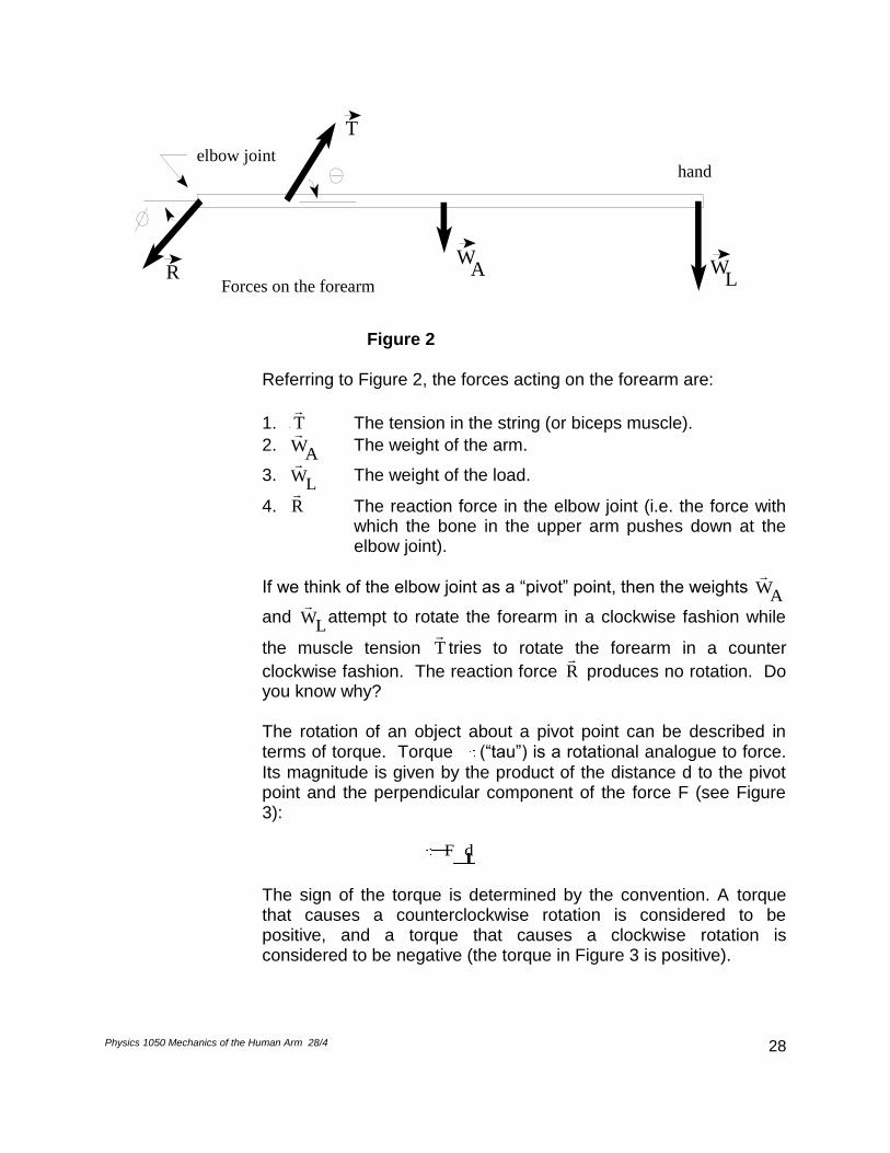
Figure 2

Referring to Figure 2, the forces acting on the forearm are:

1. T

T The tension in the string (or biceps muscle).

2. W

A The weight of the arm.

3.

WL

The weight of the load.

4. R The reaction force in the elbow joint (i.e. the force with

which the bone in the upper arm pushes down at the elbow joint).

If we think of the elbow joint as a “pivot” point, then the weights W

A

and

WL

attempt to rotate the forearm in a clockwise fashion while

the muscle tension T tries to rotate the forearm in a counter

clockwise fashion. The reaction force R produces no rotation. Do

you know why?

The rotation of an object about a pivot point can be described in terms of torque. Torque (“tau”) is a rotational analogue to force.

Its magnitude is given by the product of the distance d to the pivot point and the perpendicular component of the force F (see Figure 3):

F d

The sign of the torque is determined by the convention. A torque that causes a counterclockwise rotation is considered to be positive, and a torque that causes a clockwise rotation is considered to be negative (the torque in Figure 3 is positive).

elbow joint hand

Forces on the forearm W

W

T

R A L

Physics 1050 Angular Acceleration of a Disk 29/4 29

Figure 3

For the forearm to remain stationary, two conditions must be satisfied:

1. The forearm is not accelerating out of its elbow joint. Hence the

net force on the forearm must be zero. Resolving all of the forces on the forearm into x and y components will result in two scalar equations:

ΣFx = 0 , ΣFy = 0

2. Since the forearm is not rotating about its elbow joint, the net torque on the forearm must be zero. If we choose any pivot point, the sum of the counterclockwise torques (positive) and clockwise (negative) must be zero about that point:

Στ = 0 PROCEDURE: PART I: WEIGHT OF THE ARM

Clamp the upper beam of the apparatus to a bench and tape a protractor to the lower beam such that the origin of the protractor is aligned with the point that the string exits the top of the beam. Also ensure that the 0 degree lines on the protractor are aligned with the top of the beam. Apply enough tension in the string so that the lower arm becomes horizontal (use a level). While the lower beam is held level, adjust the biceps beam so that the string aligns with the 90o mark on the protractor. Remove the tension in the string, but ensure that the biceps beam does not move. Attach a protractor to the upper (shoulder) joint so that the 90o mark aligns with the black mark on the biceps beam. Your apparatus is now

d

F F


calibrated so that the arm is level whenever the angles on the protractors are identical. After calibration, you will mount weights on the end of the arm using a mass hanger. For 6 different loads, WL (between 0 gm and 50 gm, in steps of 10 gm), determine the string tension T required to maintain the forearm in a horizontal position. Record the weight of the load and the tension in a suitable table. Be sure to include the mass of the hanger in your calculation of the weight of the load, and note that the weights should be measured in Newtons. From each of these measurements, compute WA using rotational equilibrium. NOTES:

1) Friction gives the forearm a tendency to “stick” near equilibrium.

To account for this when making measurements, you should move the forearm to the horizontal position and see if it moves away from this position. (A light tap is also helpful).

2) The distance between the elbow joint and the tendon is 4.1±.1

cm, the distance between the elbow joint and the load is 31.4±.1 cm and the distance from the elbow joint to the centre of mass of the arm is 16.0±.1 cm.

PART II: EQUILIBRIUM OF FORCES

Remove any load from the end of the arm. Set the angle of the arm to be 50o by aligning the black mark on the bicep with this angle on

the upper protractor. Find the tension T needed to keep the

forearm horizontal by using a spring balance attached the end of the string, as in Part I. Record your result in a table. Repeat this procedure for angles between 60o and 130o, in steps of 10o. Present your results in a graph of tension vs. angle.

CAUTION: For obtuse angles (>90o) the apparatus is unstable and the arm may move upwards quickly and in the process break the string, and any fingers in the way, etc. You will observe that the forearm loses its balance very easily and seems to move either way from the horizontal position; this is called unstable equilibrium.

ANALYSIS: 1) From your data from Part 1, calculate the average weight of the

arm.

2) From your data for part 2, use translational equilibrium to find Rx


and Ry, the components of the reaction force R. These components can then be used to find the magnitude of the reaction force R. Present these results as columns in your table of tension and angle. Include the values for R as a series on your graph of tension vs angle.

DISCUSSION: 1) Are the values of T the same (within error) on the obtuse side of

90 as those on the acute side? For example, does the tension recorded at 70o equal that at 110o? Should these values be equal? Explain your answer.

2) What do you predict the tension T to be at θ = 180 ? (Do not attempt to test this experimentally!)


ANGULAR ACCELERATION OF A DISK OBJECTIVE: The objective of this experiment is to determine the relation

between torque and angular acceleration. BACKGROUND: The analogy of Newton's second law F = ma as applied to

rotational motion states that the angular acceleration of a body (α) is proportional to the torque τ and inversely proportional to the moment of inertia or rotational inertia I of the body.

τ = Iα

where [τ] = N m, [I] = kg m2 and [α] = rad/s2.

Just as the mass of a body is a measure of the tendency of the body to resist linear acceleration, so the moment of inertia is a measure of a body's resistance to angular acceleration. If a body is free to rotate about an axis, then a torque is required to change the rate of rotation. The resulting angular acceleration is proportional to the torque as per Eq. (1) and exists only during the time the torque acts on the body.

The moment of inertia of a body is dependent on the mass of the body and the distribution of the mass about the axis of rotation. To determine I, the body is divided into a number of infinitesimal elements mi, each at some distance ri from the axis of rotation. The moment of inertia is given by the sum of all the products miri

2

calculated for each element. If the body is a simple geometric shape, e.g., a disk, sphere, or cylinder, I can be easily calculated; results for such calculations are given in tables. For a solid disk the expression is

where M is the total mass of the disk and R its radius.

In this experiment the linear acceleration a of a mass m suspended on a cord is measured. This cord is wound around the hub of the disk (see Fig. 1) and as a result, the magnitude of the linear

I =

n

i=1

mir2

i

I = 1

2 MR2


acceleration of the rim of the hub is also a.

Figure 1

Where m is the mass of the falling weight and S is the tension in the cord.

By calculating the linear acceleration on the rim we can determine the angular acceleration α of the hub (which is also the angular acceleration of the disk) through the equation

where r is the radius of the hub.

The torque τ (a vector) resulting from a force F applied about an axis is given by the expression:

In this experiment the torque is supplied by the tension in the cord from which the mass is suspended(see Fig. 1).

α = ar,

τ = (r)(F) sin θ.


The torque can be calculated as,

and is considered to be a vector pointing into the paper.

Combining Eqs. (1) and (6), we obtain

Applying Newton's second law to the linear motion of the falling weight we can write

Eliminating S in Eqs. (7) and (8) yields,

A plot of (mgr - mr2

α) vs α should yield a straight line with slope I, assuming the frictional torque is constant.

PROCEDURE: 1. Using six different weights, record the time taken for the weight

holder to fall a measured distance d, where

2. The time may be measured by using stop watches. If this

method is used, you may wish to team up with another group to gather the data. This would allow 3 or 4 people to simultaneously time each run. Do at least 2 trials for each run.

3. Record the following information for each run: mass, time,

distance fallen.

ANALYSIS: Construct the following table, using the information contained in this

manual to calculate values for and .

τ = rS sin 90o = rS

S=Iα

r

S = mg - ma

mgr - mr2α = Iα

d = 1

2at2.

Physics 1050 Speed of Sound 35/6 35

Plot a graph of (mgr - mr2

α) vs. α. The slope of this graph is the experimental value of the moment of inertia (Iexp). Compute the theoretical moment of inertia as follows:

where

Md = mass of disk Rd = radius of disk Mh = mass of hub Rh = outer radius of hub rh = inner radius of hub.

Compare Iexp with Ith, and record the percentage difference between the 2. Do these two values agree within reason?

DISCUSSION TOPICS:

Should the line for Iexp pass through the origin of your plot?

Think of an experiment that could be used to measure the frictional torque present in this apparatus. This experiment can not involve taking apart the apparatus.

Falling Mass

(kg)

Average Time

of Fall (s)

Angular

Acceleration(α) (rad/s2)

Torque

(mgr - mr2α) (N-m)

Ith =

MdR2

d + M

h(R

2

h + r

2

h)

2,


PRINCIPLES OF MECHANICS

OBJECTIVE: The objective of this experiment is to illustrate several principles of mechanics using a simple collision as an example.

APPARATUS: Ramp Ball Bearing Paper Meter Stick(s) Carbon Paper BACKGROUND: This simple experiment provides an opportunity to apply a variety of

mechanical principles.

We will roll a ball down an incline and examine its path as it flies, strikes the floor, and bounces. With a few simple distance measurements we should be able to examine momentum, energy, projectile motion, kinematics, impulse and collisions.

PROCEDURE: Figure 1 depicts the experimental set-up and measurements to be

made.

Figure 1.

H

h

A

D e

c d

recording paper

B

C


Obtain a ramp from your instructor. Place the ramp on a lab bench with the end of the ramp parallel to the floor (shim the stand if necessary), and clamp it in place. Roll the ball bearing down the ramp, allow it to hit the floor and bounce. Place a large sheet of paper on the floor (tape it down) such that the bearing will strike the paper on impact and first bounce (points C and D in Figure 1). Measure the heights h and H and record them. Measure the mass (m) of the ball using the scales at the back of the lab.

Data for this experiment is collected by releasing the ball several times from the same spot on the ramp. If the carbon paper is placed at points C and D, then each time the bearing strikes the paper it will leave a mark. For each trial mark the impact sites with a number. Do a total of 5 trials and find the average of lengths d and c. The height (e) of the bounce can then be found by placing a piece of paper mounted on a book mid-way between points C and D. Place the leading edge of the book exactly at the midway point and do more 5 more trials. The ball will leave a mark on the paper at the maximum height. Record these heights and use the average value as your value for e.

Before you dismantle your apparatus be sure you have made measurements of all the dimensions shown in figure 1 (c,d,e,H,h, and the mass m of the ball bearing).

ANALYSIS: Using kinematics, calculate the following quantities:

1. The time required for the ball to strike the ground after leaving the ramp.

2. The speed of the ball as it leaves the ramp (point B). Note

that this speed is the horizontal velocity of the ball, which can be calculated using the time from question 1 and the distance the ball travelled before reaching the ground (c).

3. The vertical velocity as the ball strikes the ground (point C).

4. The speed at point C.

5. The speed at point D. By examining the path of the ball from

the maximum height of the bounce to point D, this problem is solved in an identical manner to questions 1-4.


Using these values for the speeds, construct a table that lists the kinetic, potential, and total mechanical energy at points A, B, C, and D. Your table should resemble the following:

Height Speed KE PE Mech Energy

A

B

C

D

Calculate the speed of the ball at point C using energy considerations. Does it agree with the result you found using kinematic methods?

DISCUSSION: Is the mechanical energy in this experiment conserved? If not, where is it lost? In particular, is the collision at point C elastic or inelastic?

To this point we have not considered the energy of rotation as the ball rolls down the ramp. The kinetic energy of rotation (Krot ) can be calculated as,

Krot = ½ I ω2,

where I is the moment of inertia ( I = 2/5 mr2 for a solid sphere),

and = v / r is the angular velocity. By substituting these

expressions for I and into the equation for Krot, find an equation for Krot that is a function of mass and speed. Using the speed from question 2 (the speed as the ball leaves the ramp), calculate this rotational energy. Now add this number to the energies at points B and C. Does the inclusion of the energy of rotation in your calculation reconcile the differences in the mechanical energies at A, B, and C?


CONSERVATION OF MOMENTUM OBJECTIVE: The objective of this experiment is to study the vector nature of

momentum and the principle of conservation of momentum by colliding two gliders on an air track.

APPARATUS: Air Track with two gliders

Dual Beam Sonar System BACKGROUND: In this experiment two gliders will be set in motion on the air track

such that they collide with each other and the ends of the air track several times. The sonar system will track the position of each glider. The interactions of the gliders with each other and the ends of the air track are such that conservation of momentum can only be demonstrated by the use of vectors.

The momentum of an object is a vector quantity defined as the product of the mass and the velocity of the object:

mvp .

In a system of objects (1,2,3,...,n), the total momentum P of the system is simply the vector sum of the individual momenta.

nppppP ...321 .

The motion of the system (gliders on the air track) is in one dimension, therefore the vector part of the momentum can be handled with the use of +/- signs. Under the proper conditions(no external forces etc.) the momentum of the system should remain constant and we can write:

fi pppp )()( 2121 ,

where i stands for "initial" or before collision and f stands for "final" or after collision.

In this experiment we will put two gliders in motion on the air track such that they collide(elastically) with each other and the ends of the air track several times.


PROCEDURE: 1. Weigh the two gliders to be used in the experiment( one glider must have a tall sonar target while the other a shorter one).

2. Use the "SR" program located in the “physics” subdirectory. Set the data collection menu to "Two Targets."

3. Adjustment of the sonar head is critical in this experiment, both

traces should be free of noise. Do not stand too close to the air track while making adjustments or during the experiment as this will cause echoes to be picked up by the sonar system.

4. When all adjustments have been made obtain a sonar plot of

the gliders as they move along the air track. A good trace will resemble this one:

The traces represent the distance of each glider from the sonar head as a function of time. Since the sonar head is located at one end of the air track, the upper trace was made by the glider furthest away from the sonar head (far glider) and the lower


trace by the glider nearest the sonar head (near glider). The peaks on the top trace are indicative of collisions between the far glider and the far end of the air track. The valleys on the lower trace indicate collisions between the near glider and the near end of the air track. The peaks of the lower trace and the valleys of the upper trace always occur at the same time and therefore indicate collisions between the two gliders.

5. Save your data on your disk using the Load/Save menu.

ANALYSIS: 1. Set-up a data table in which you calculate the momentum of

each glider and the total momentum of the system.

2. Plot the total momentum and the position data for each glider on a single graph as functions of time.

3. Examine the total momentum trace very carefully and give a

detailed explanation of its appearance.


THE SPEED OF SOUND

OBJECTIVE: The objective of this experiment is to determine the speed

of sound in air. APPARATUS: Function Generator

Oscilloscope Tool Box Resonance Tube Kit

BACKGROUND: Waves

The repetitive motion of waves breaking on a beach is probably the most familiar concept we have of waves. This familiar concept can be extended to represent many processes that occur in nature. Physical terms such as frequency (f in cycles/sec, or Hz), wavelength (λ in cm or m), phase (υ in radians), and amplitude (magnitude of process represented by the wave) can be employed to quantify and measure properties in other cyclical processes which behave like the conceptually familiar water waves.

Terms such as node and antinode are also used to identify particular positions on the wave. Nodes represent points on the wave where the value of the process depicted by the wave is at a minimum. Conversely, antinodes are points depicting the maximum ( positive or negative) value of the process depicted by the wave. For example if the wave shown above represented 110 volt household AC electricity, then the amplitude would represent voltage (maximum value of about 155 volts at the antinodes). The frequency of the wave would be 60 Hz and the value of the voltage at the nodes would be 0 volts.

wavelength

node

amplitude

antinode


Waves propagate from one place to another at a speed which can be defined as the frequency of the wave multiplied by the

wavelength of the wave, v = fλ.

Sound Waves

Sound waves are longitudinal waves, meaning that the direction of

the „oscillation' is parallel to the direction of propagation of the wave. The speed at which the wave travels (propagation velocity) is dependent on the medium through which the wave is travelling. In a simple sense the stiffer the medium the faster the speed of sound.

One indicator of „stiffness‟ in materials or media is the bulk modulus (B). When combined with the density of the medium (ρ), the speed of sound (V) may be calculated as:

V

Typical values of B and ρ :

Material Bulk Modulus (Pa) Density (kg/m3) Water 0.21 X 1010 1.0 X 103 Steel 20 X 1010 7.8 X 103 Aluminum 7 X 1010 2.7 X 103

Propagation of sound in a gas is a slightly more involved subject. Ignoring the details, the equation for calculating the speed of sound in a gas is:

V RT

M

where:

γ = a constant particular to individual gases R = the gas constant (8.314 J mol-1 K-1) T = the absolute temperature (K) M = the molecular mass of the gas (Kg/mol)


Typical values of γ and M :

Gas γ M (Kg/mol) Air 1.40 .0288 Helium 1.67 .0040 CO2 1.30 .0280

If one considers the speed of sound in air then factors such as altitude, humidity, and pressure also enter into the calculation for the speed of sound.

A sound wave consists of alternating pressure changes called compressions and rarefactions. As the wave moves it compresses the air to a pressure greater than atmospheric pressure. Between successive compressions there is a region of low pressure called a rarefaction. The compressions and rarefactions occur along the path the wave is travelling.

Audible sounds travelling through air will have wavelengths ranging from approximately 3 to 300 cm. Wavelengths of this size are easy to study. We will employ sound resonance in a tube to determine the wavelength of the sound waves (λ), determine the frequency (f) of the sound wave with an oscilloscope frequency, consequently calculating the speed of the wave as the product of f and λ .

Superposition Observations of waves in nature reveal that waves interact with each other in special ways. If you throw two stones into a pond for example, and watch the wave pattern created by each, you will observe that the patterns interact with each other in passing, but the individual patterns remain intact and continue to propagate after the interaction.

These observations are indicative of the principle of superposition. Multiple waves may interact with each other without losing their individual character. The interaction is generally referred to as interference. For our purposes the interaction of sound waves in this experiment will be considered to be linear.

Superposition of sound waves moving through air can be very complicated. The air molecules are already moving in a random motion. As a sound wave(s) travels it imposes an ordered vibrational motion on the already moving molecules. The motion of a molecule at any instant will be a combination of random motion


and the oscillations caused by any number of sound waves present at that instant.

Resonance

The principle of superposition leads to a phenomenon known as resonance. In this experiment sound resonance occurs when the wavelength of the sound “fits” the cavity in which it is travelling. Consider a long tube closed at one end. A sound wave enters the open end and travels along the tube until it hits the closed end. Upon striking the closed end the sound wave reverses direction (reflection) and travels back down the tube toward the open end.

When a wave is reflected in this manner there is a 180 phase change in the wave; this is a very important factor for resonance.

Figure 2

By adjusting the frequency, and therefore the wavelength of the sound, it is possible to create standing waves in the tube. As you can see in Figure 2, if a node occurs at the closed end of the tube

then the reflected wave is 180 out of phase with the incoming wave. If the wavelength is such that an antinode is located at the mouth of the tube then we have the proper conditions for a standing wave. Each wave travelling in the tube will reflect back upon itself without altering the positions of the nodes and antinodes. The conditions for a standing wave are also the conditions for resonance. The resulting interaction of the sound waves in the tube is the addition of their respective amplitudes (sound) thereby


making a much louder sound than that of any single wave in the tube. You can also see from the Figure 2 that only odd multiples of λ/4 can produce resonance in the tube and distance between successive resonances for a tube of length L will be λ/2.

PROCEDURE: Obtain a function generator, resonance tube kit, tool box, and

oscilloscope. Assemble them as directed by the instructor using the set-up at the front of the lab as a guide. Your instructor will assist you with any difficulties and demonstrate how to use the oscilloscope and function generator.

Typical Resonance Tube Set-up

There are many ways to use this apparatus to determine the speed of sound (your instructor will demonstrate some of them). One method involves selecting a fixed frequency and adjusting the length of the tube to find lengths at which the tube resonates. Alternatively, one could select a particular length for the tube and vary the frequency to produce resonance in the tube. This experiment will use the first method.

The experiment will comprise three trials at different frequencies. For each trial, start with the moveable piston at the zero mark on the scale. With the microphone located next to the speaker slowly move the piston away from the speaker and observe the oscilloscope screen. The wave on the oscilloscope screen is the signal from the microphone. Its height represents the magnitude of the sound inside the tube. The height of the wave will rise and fall depending on the length of the tube. When the tube is at a length that corresponds to


a resonance for the frequency in question the wave will have its maximum height. Record each length for which a maximum occurs.

Since this is a closed tube each resonance occurs at nλ /4, where n = 1,3,5,7,... . The change in the measured distances is half a wavelength. The frequency of the signal can be measured with the oscilloscope.

Pick three different frequencies in the range of 1000 to 3000 Hz. For each frequency alter the length of the tube using the moveable piston Each time the tube comes into resonance record the length (L) of the tube by noting the position of the piston on the scale. Record your results in a simple table:

Frequency Length Wavelength

Speed

ANALYSIS: 1. Report the speed of sound for each trial as the average of your

calculations ± the standard deviation of the average. Calculate the overall speed of sound as the average of all calculations ± the standard deviation of the overall average.

2. Using the information from the background section of the lab

outline plot a graph of the speed of sound in air from -40o C to +40o C.

3. How many times faster does sound travel in steel than in water?

DISCUSSION: In practice the diameter of the tube used in the experiment also has

an effect on the calculated speed of sound. The actual wavelength of the sound is calculated as L + 0.4d = nλ /4, where L is the measured length of the tube and d is the diameter of the tube. What consequences does this have for your calculated speed of sound?

Physics 1050 Nuclear Half-Life 48/5 48

NUCLEAR HALF-LIFE OBJECTIVE: To determine the half-life of 137Ba. WARNING: No food or refreshments are allowed in the lab during this experiment. APPARATUS: Ba -137 Liquid Sample Geiger Tube BACKGROUND: Most elements present in nature exist in more than one nuclear

configuration. The slightly different configurations of an element are known as isotopes. Consider neon which has several different natural forms:

10Ne20 10Ne21 10Ne22.

The atomic number (10) identifies each as being the element neon, while the mass number denotes differing numbers of neutrons in the respective nuclei (20, 21, 22). Other isotopes of neon exist, ie.:

10Ne18 10Ne19 10Ne24 .These have half-lives ranging from 1.5 sec to 3.38 min.

Unstable isotopes rearrange themselves into stable configurations primarily through nuclear emission. In this experiment we will study some of the emission characteristics of various isotopes, shielding properties of various materials, and examine different detection methods.

Types of We are interested in three types of radioactive nuclear emission: Nuclear Radiation Alpha (α). These are positive particles which are identical to

helium nuclei except for their nuclear origin. They travel about 0.1 the speed of light and possess great ionizing power because of their relatively slow speed and great charge. All the alpha particles emitted from a given species of nucleus are mono-energetic (identical in energy). Alpha particles may be stopped by a thin sheet of paper.

Beta (β). Unlike alpha particles, they are negatively charged and are identical to the electron except for their nuclear origin. Commonly encountered beta particles travel up to 0.9 the speed of light. Unlike alpha particles, beta particles are emitted in a wide range of energies, hence the variation in their speed. Beta particles are more penetrating than alpha particles but may be stopped by several thin sheets of metal.


Gamma (γ). Gamma emission is similar to x-rays and light rays but have a shorter wave length. These rays are emitted because of energy transitions within the nucleus itself, while x-rays are emitted because of energy transitions in orbital electrons. Since gamma rays have no charge, they do not react with matter in the same manner as alpha and beta particles. They travel at the speed of light and have great penetrating power.

Nuclear While it is impossible to predict which nucleus in a collection of Emission radioactive nuclei will decay next, it is possible to establish the rate

at which the collection of nuclei decays. It can be shown that a collection of N radioactive nuclei will decay at a rate proportional to the number of nuclei yet to undergo emission in the sample. The rate of decay is characteristic of the isotope in question and can be expressed either as the half-life (T1/2) or the mean life (τ) of the isotope.

Mathematically the rate of decay (R) is expressed as,

R = λN, (1) where N is the number of nuclei yet to undergo decay and λ is the decay constant characteristic of a particular radionuclide. The rate of decay as a function of time follows an exponential pattern expressed as,

R = Ro e -λt (2) where Ro is the rate of decay at t = 0.

Nuclear Decay of a Radio Active Isotope

Time

Ro


By taking the natural log of both sides of equation 2 a linear relationship results which can be used to determine λ.

ln(R) = -λt + ln(Ro) (3)

Figure 2

λ can found by calculating slope of the plot in figure 2.

The rate at which a sample decays is called the activity and carries the SI unit of becquerel (Bq). One becquerel is one decay per second. Another unit of nuclear decay rate is the curie (Ci). One curie is 3.7 X 1010 Bq. When it is not clear whether a detector is recording all the disintegrations from a sample it is common practice to use units of counts per unit time.

Nuclear The half-life (T1/2) of a radionuclide is a measure of how long a Half-Life particular isotope will continue to decay. The value of the half-life of

an isotope is the time required for the initial rate of decay ( can be any value) to drop to one half that rate.

The half-life of a radionuclide is calculated by relating the decay constant to the time for one half of the nuclei in a sample to disintegrate.

½ Ro = Ro e-λT1/2 (4)

Nuclear Decay of a Radio Active Isotope

Time


Taking the natural logs of each side of this equation yields an expression for the half-life of a radionuclide.

T1/2 = ln(2) / λ (5)

137Ba The Barium isotope used in this experiment is generated from the beta decay of 137Cs with a half-life of 30 years. At this point the 137Ba nucleus is unstable and quickly undergoes a decay by gamma emission (662 KeV) to become stable. The half-life determined in this experiment is the half-life of the gamma decay to form stable 137Ba.

PROCEDURE: You will be given a liquid sample of 137Ba on a planchette. This

isotope decays quickly so you must be ready to work as soon as the sample is received.

1) Place the sample under the GM tube.

2) Using the Geiger program on the computer, collect data for 600 seconds.

3) Every 30 seconds, record the number of counts.

137 Cs (30.1 y)

137 Ba ( unstable)

137 Ba (stable)

1.174 MeV

Emission

0.512 MeV

Emission

0.662 MeV

Emission

Physics 1050 Nuclear Shielding 52/3 52

4) Find the number of counts within each 30 second interval by

finding the difference between consecutive measurements of the number of counts.

ANALYSIS: 1) Construct a data table of the number of counts within each

30 second interval as a function of time.

2) Construct a plot of the number of counts as a function of time.

3) Construct a plot of the natural log of the number of counts as

a function of time. The slope of this line is the decay

constant ( ) for this isotope. Using linear regression, find this slope.

4) Use equation (5) to calculate the half- life using the value of

obtained from step 4.

physics 1050 lab manual spring 2010

Documents