physics 100 lab 1: introduction to motion - sfu.camxchen/phys100/p100labs.pdf · page 1-2 real time...

Name Sec: Last 2 Digits of St# Partners: Date:

©1993-94 P. Laws, D. Sokoloff, R. ThorntonSupported by National Science Foundation and U.S. Department of Education (FIPSE)Note: These materials have been edited at Simon Fraser University by N. Alberding

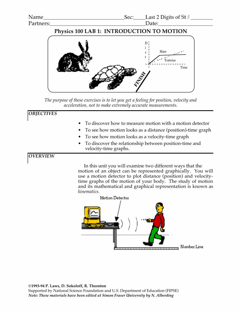
Physics 100 LAB 1: INTRODUCTION TO MOTION

Dist

Time

Tortoise

Hare

FINISH

The purpose of these exercises is to let you get a feeling for position, velocity andacceleration, not to make extremely accurate measurements.

OBJECTIVES

• To discover how to measure motion with a motion detector• To see how motion looks as a distance (position)-time graph• To see how motion looks as a velocity-time graph• To discover the relationship between position-time and

velocity-time graphs.OVERVIEW

In this unit you will examine two different ways that themotion of an object can be represented graphically. You willuse a motion detector to plot distance (position) and velocity-time graphs of the motion of your body. The study of motionand its mathematical and graphical representation is known askinematics.

2 Real Time Physics: Active Learning Laboratory V1.40--8/94

©1993-94 P. Laws, D. Sokoloff, R. ThorntonSupported by National Science Foundation and U.S. Department of Education (FIPSE)

INVESTIGATION 1: DISTANCE (POSITION)-TIME GRAPHS OF YOUR MOTION

The purpose of this investigation is to learn how to relategraphs of distance as a function of time to the motions theyrepresent.You will use the following materials:

• Logger Pro® software• Physics 100 Experiments folder• Go!Motion® motion detector• Number line on floor in meters (optional)

How does the distance-time graph look when you move slowly?Quickly? What happens when you move toward the motiondetector? Away? After completing this investigation, youshould be able to look at a distance-time graph and describe themotion of an object. You should also be able to look at themotion of an object and sketch a graph representing thatmotion.Comment: "Distance" is short for "distance from the motion detector."The motion detector is the origin from which distances are measured.• It detects the closest object directly in front of it

(including your arms if you swing them as you walk).• It will not correctly measure anything closer than 0.15

meter. (When making your graphs don't go closer than 0.15 meter from the motion detector.)

• As you walk (or jump, or run), the graph on the computer screen displays how far away from the detector you are.

Activity 1-1: Making Distance-Time Graphs (should take about 5 minutes)1. Make sure the computer is turned on and the Physics 100

folder is visible. (Ask a TA to help if it isn’t) Use the mouseto click on the file L1 #1.cmbl. The graph axes should appearon the screen. (Be sure the motion detector is plugged into aUSB port at the back of the computer.)

2. When you are ready to start graphing distance, click once onthe green “Collect” button in the top middle of the screen.

3. If you have a number line on the floor or on the edge ofyour bench, and you want the detector to produce readingsthat agree, stand at the 2-meter mark on the number line andhave someone move the detector until the reading is 2 m.

4. Make distance-time graphs for different walking speeds anddirections, and sketch your graphs on the axes.

Real Time Physics: Lab 1: Introduction to MotionPage 1-3Authors: David Sokoloff, Ronald Thornton & Priscilla Laws V1.40--8/94


a. Start at the 1/2-meter markand make a distance-timegraph, walking away fromthe detector (origin) slowlyand steadily.

Time (seconds)

Dist

ance

(met

ers)

b. Make a distance-time graph,walking away from thedetector (origin) medium fastand steadily.

Time (sec)

Dist

ance

(m)

c. Make a distance-time graph,walking toward the detector(origin) slowly and steadily.

Time (sec)

Dist

ance

(m)

d. Make a distance-time graph,walking toward the detector(origin) medium fast andsteadily.

Time (sec)D

istan

ce (m

)Comment: It is common to refer to the distance of an object fromsome origin as the position of the object. Since the motion detector isat the origin of the coordinate system, it is better to refer to the graphsyou have made as position-time graphs. From now on you will plotposition-time graphs.

Activity 1-2: Matching a Position Graph (approx. 10 min)By now you should be pretty good at predicting the shape of agraph of your movements. Can you do things the other wayaround by reading a position-time graph and figuring out howto move to reproduce it? In this activity you will match aposition graph shown on the computer screen.1. Open the experiment file called L1 #2 (Position Match).cmbl

from the Physics 100 folder. A position graph like thatshown below will appear on the screen.Comment: This graph is stored in the computer as Match Data.

New data from the motion detector are always stored as Latest Run,and can therefore be collected without erasing the Position Matchgraph.



4 8 12 16 200

--

--4

0

2

. . . . .

. . . . .. . . . .

. . . . .

Time (seconds)

Posit

ion

(m)

Clear any data remaining from previous experiments inLatest Run by selecting Clear Latest Run from theExperiment Menu.

2. Move to match the Position Match graph on the computerscreen. You may try a number of times. It helps to work in ateam. Get the times right. Get the positions right. Eachperson should take a turn. Sketch the best attempt on thegraph.

INVESTIGATION 2: VELOCITY-TIME GRAPHS OF MOTION

You have already plotted your position as a function of time.Another way to represent your motion during an interval oftime is with a graph, which describes how fast and in whatdirection you are moving. This is a velocity-time graph. Velocityis the rate of change of position with respect to time. It is aquantity, which takes into account your speed (how fast you aremoving) and also the direction you are moving. Thus, whenyou examine the motion of an object moving along a line, itsvelocity can be positive or negative meaning the velocity is inthe positive or negative direction.Graphs of velocity vs. time are more challenging to create andinterpret than those for position. A good way to learn tointerpret them is to create and examine velocity-time graphs ofyour own body motions, as you will do in this investigation.

Activity 2-1: Making Velocity Graphs (approx. 5 min)1. Set up to graph velocity. Open the experiment L1 #3

(Velocity Graphs). Make sure that the Velocity axis is set toread from -1 to 1 m/sec and the Time axis from 0 to 5 sec, asshown on the next page.



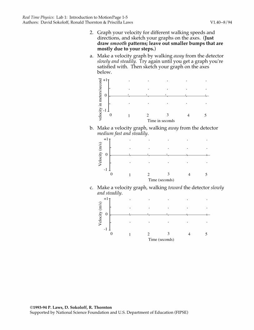
2. Graph your velocity for different walking speeds anddirections, and sketch your graphs on the axes. (Justdraw smooth patterns; leave out smaller bumps that aremostly due to your steps.)

a. Make a velocity graph by walking away from the detectorslowly and steadily. Try again until you get a graph you'resatisfied with. Then sketch your graph on the axesbelow.

2 3 4 5-1

+1

0

0

. . . . .

. . . . .

. . . . .

. . . . .

---

- - - - -

1Time in secondsve

loci

ty in

met

ers/s

econ

d

b. Make a velocity graph, walking away from the detectormedium fast and steadily.

2 3 4 5-1

+1

0

0

. . . . .

. . . . .

. . . . .

. . . . .

---

- - - - -

1

Vel

ocity

(m/s)

Time (seconds)

c. Make a velocity graph, walking toward the detector slowlyand steadily.

2 3 4 5-1

+1

0

0

. . . . .

. . . . .

. . . . .

. . . . .

---

- - - - -

1

Vel

ocity

(m/s)

Time (seconds)



d. Make a velocity graph, walking toward the detectormedium fast and steadily.

2 3 4 5-1

+1

0

0

. . . . .

. . . . .

. . . . .

. . . . .

---

- - - - -

1

Vel

ocity

(m/s)

Time (seconds)

*** IMPORTANT Comment: You may want to change the velocityscale so that a graph fills more of the screen and is clearer. To do this,use the mouse to double click anywhere on the graph and change thevelocity range in the dialog box. Another way to do this is to click themouse once with the cursor pointing to the maximum axis reading.Type in the new value and hit return.

Activity 2-2 Predicting a Velocity Graph (approx. 5 min)Prediction 2-1: Predict a velocity graph for a more complicatedmotion and check your prediction.Each person draw below, using a dashed line your prediction ofthe velocity graph produced if you:

• Walk away from the detector slowly and steadily forabout 5 seconds, then stand still for about 5 seconds, thenwalk toward the detector steadily about twice as fast asbefore

Compare your predictions and see if you can all agree. Use asolid line to draw in your group prediction.(To get desired scaling on the axis, read Comment above)

PREDICTION

Vel

ocity

(m/s)

Time (seconds)3 6 9 12 15

-1

+1

0

0

. . . . .

. . . . .

. . . . .

. . . . .

-

-

-

- - - - -



3. Test your prediction. (Be sure to adjust the time scale to 15seconds. As before, this can be done by clicking the mouseonce on the 5 to highlight it, typing in a 15 and then hittingthe return key. ) Repeat your motion until you think itmatches the description.Draw the best graph on the axes below. Be sure the 5-second stop shows clearly.

FINAL RESULT

Vel

ocity

(m/s)

Time (seconds)3 6 9 12 15

-1

+1

0

0

. . . . .

. . . . .

. . . . .

. . . . .

-

-

-

- - - - -

INVESTIGATION 3: RELATING POSITION AND VELOCITY GRAPHS

Since position-time and velocity-time graphs are differentways to represent the same motion, it ought to be possible tofigure out the velocity at which someone is moving byexamining her/his position-time graph. Conversely, you oughtto be able to figure out how far someone has traveled (change inposition) from a velocity-time graph.

Activity 3-1: Predicting Velocity Graphs from Position Graphs(approx 10 min)

1. Set up to graph Position and Velocity. Open the experimentL1 #5 (Velocity from Position) to set up the top graph todisplay Position from 0 to 4 m for a time of 5 sec, and thebottom graph to display Velocity from -2 to 2 m/sec for 5sec. Clear any previous graphs.

Prediction 3-1: Predict a velocity graph from a position graph.Carefully study the position-time graph shown below andpredict the velocity-time graph that would result from themotion. Using a dashed line, sketch your prediction of thecorresponding velocity-time graph on the velocity axes.



–2

+2

0

. . . . .

.2

. . .

. . . . .

---

. . . . .4

. . . . .

1 3 4 5

00

. . . . .

. . . . .

. . . . .

-

2-

Time (seconds)

2. Test your prediction. After each person has sketched aprediction, Collect, and do your group's best to make aposition graph like the one shown. Walk as smoothly aspossible.When you have made a good duplicate of the positiongraph, sketch your actual graph over the existing position-time graph.Use a solid line to draw the actual velocity graph on the samegraph with your prediction. (Do not erase your prediction).

Activity 3-2: Calculating Average Velocity (approx 10 min)In this activity, you will find an average velocity from yourvelocity graph in Activity 3-1 and then from your positiongraph.1. Find your average velocity from your velocity graph in

Activity 3-1. Select Examine in the Analyze menu, read anumber of values (say five) from the portion of your velocitygraph where your velocity is relatively constant, and use them tocalculate the average (mean) velocity. Write the five valuesin the table below.

12345

Velocity Values (m/s)

Average value of the velocity: ________m/s



Comment: Average velocity during a particular time interval can alsobe calculated as the change in position divided by the change in time.(The change in position is often called the displacement.) By definition,this is also the slope of the position-time graph for that time period.As you have observed, the faster you move, the more inclined is yourposition-time graph. The slope of a position-time graph is aquantitative measure of this incline, and therefore it tells you thevelocity of the object.

2. Calculate your average velocity from the slope of yourposition graph in Activity 3-1. Use Examine to read theposition and time coordinates for two typical points whileyou were moving. (For a more accurate answer, use twopoints as far apart as possible but still typical of the motion,and within the time interval over which you took velocityreadings in (1).)

Position (m) Time (sec)Point 1Point 2

Calculate the change in position (displacement) betweenpoints 1 and 2. Also calculate the corresponding change intime (time interval). Divide the change in position by thechange in time to calculate the average velocity. Show yourcalculations below.

Change in position (m)Time interval (sec)Average velocity (m/s)

Activity 3-3: Predicting Position Graphs from Velocity Graphs (approx 10 min)

Prediction 3-2: Carefully study the velocity graph shownbelow. Using a dashed line, sketch your prediction of thecorresponding position graph on the bottom set of axes.(Assume that you started at the 1-meter mark.)



2 4 6 8 100

4

0

2

. . . . .

. . . . .

. . . . .

. . . . .

-

-

-

-1

+1

0

. . . . .

. . . . .

. . . . .

-

-

-

Time (seconds)

. . . . .

PREDICTION AND FINAL RESULT

Test your prediction.1. Open the experiment L1 #6 (Position from Velocity).2. After each person has sketched a prediction, do your group's

best to duplicate the top (velocity-time) graph by walking.Be sure to graph velocity first.When you have made a good duplicate of the velocity-timegraph, draw your actual result over the existing velocity-time graph.

3. Use a solid line to draw the actual position-time graph on thesame axes with your prediction. (Do not erase yourprediction.)



Study questions may be answered after the labInvestigation 1

1-1: Describe the difference between the graph you made by walkingaway slowly and the one made by walking away more quickly.

1-2: Describe the difference between the graph made by walking towardand the one made walking away from the motion detector.

1-3: Describe the motions that you did to match the graph in Activity 1-2.

Investigation 2

2-1: What is the most important difference between the graph made byslowly walking away from the detector and the one made by walkingaway more quickly?

2-2: How are the velocity-time graphs different for motion away from thedetector compared to those for motion towards the detector?

2-3: Describe how you moved1) when the velocity line was above horizontal zero line.

2) when the velocity line was crossing the horizontal zero line

3) when the velocity line was below zero.

2-4: Is it possible for an object to move so that it produces an absolutelyvertical line on a velocity time graph? Explain.

2-5: Did you run into the motion detector on your return trip? If so, whydid this happen? How did you solve the problem? Does a velocitygraph tell you where to start? Explain.



Investigation 3

3-1: How would the position graph be different if you moved faster?Slower?

3-2: How would the velocity graph be different if you moved faster?slower?

3-3: Is the average velocity positive or negative? Is this what youexpected?

3-4: Does the average velocity you calculated from the position graphagree with the average velocity you found from the velocity graph?Do you expect them to agree? How would you account for anydifferences?

3-5: How can you tell from a velocity-time graph that the moving objecthas changed direction?

3-6: What is the velocity at the moment the direction changes (i.e, the signof v changes from positive to negative)?

3-7: Is it possible to actually move your body (or an object) to makevertical lines on a position-time graph? Why or why not? Whatwould the velocity be for a vertical section of a position-time graph?

3-8: How can you tell from a position-time graph that your motion issteady (motion at a constant velocity)?

3-9: How can you tell from a velocity-time graph that your motion issteady (constant velocity)?

Name: Sec: Last 2 digits of St#:Partners: Date:


PHYSICS 100 LAB 2: CHANGING MOTION

A cheetah can accelerate from 0 to 50 miles per hour in 6.4 seconds.Encyclopedia of the Animal World

A Jaguar automobile can accelerate from 0 to 50 miles per hour in 6.1 seconds.World Cars

OBJECTIVES

• To discover how and when objects accelerate• To understand the meaning of acceleration, its magnitude and direction• To discover the relationship between velocity and acceleration graphs• To learn how to represent velocity and acceleration using vectors• To learn how to find average acceleration from acceleration graphs• To learn how to calculate average acceleration from velocity graphs

OVERVIEW

When the velocity of an object is changing, it is also importantto know how it is changing. The rate of change of velocity withrespect to time is known as the acceleration.

2 Real Time Physics: Active Learning Laboratory V1.40−−8/94


IN ORDER TO GET A FEELING FOR ACCELERATION, IT IS HELPFUL TO CREATEAND LEARN TO INTERPRET VELOCITY-TIME AND ACCELERATION-TIMEGRAPHS FOR SOME RELATIVELY SIMPLE MOTIONS OF A CART ON A SMOOTHRAMP OR OTHER LEVEL SURFACE. YOU WILL BE OBSERVING THE CART WITHTHE MOTION DETECTOR AS IT MOVES WITH ITS VELOCITY CHANGING AT ACONSTANT RATE. INVESTIGATION 1: VELOCITY AND ACCELERATIONGRAPHS

In this investigation you will be asked to predict and observethe shapes of velocity-time and acceleration-time graphs of acart (or toy car) moving along a smooth ramp which is slightlytilted. You will focus on cart motions with a steadily increasingvelocity.

Activity 1-1: Speeding Up

1. Set up the cart on the ramp, with the ramp tilted by placing asmall block under the end nearest the motion detector.

.5 m← ←

end stop

2. Open the experiment L2A1-1 (Speeding Up) to display atwo graph layout with Position from 0 to 2.0 m and Velocityfrom -1.0 to 1.0 m/sec for a time interval of 3.0 sec, as shownon the next page.Use a position graph to make sure that the detector can "see"the cart all the way to the end of the ramp. You may need totilt the detector up slightly.

Real Time Physics: Lab 2: Changing Motion Page 2-3Authors: D. Sokoloff, R. Thornton & P. Laws (modified by R. Morse and Neil Alberding) V1.40−−5/99


3. Hold the cart, press Collect, and when you hear the clicks ofthe motion detector, release the cart from rest. Do not put yourhand between the cart and the detector. Be sure to stop thecart before it hits the end stop.Repeat, if necessary, until you get a nice set of graphs.Change the position and velocity scales if necessary so that thegraphs fill the axes. Store the data by selecting Store LatestRun under Experiment. Then click on Data-> Data SetOptions->Run1 to change the name of the data set toSpeedUp1_xxx where xxx is your initials. Each person in thisgroup should have their own data set. Hide your saved dataset by selecting your data set under Data->Hide Data Setsbefore your partner repeats the same experiment. This wayyour and your partner’s graphs will not overlap.Sketch your position and velocity graphs neatly on the axeswhich follow. Label the graphs "Speeding Up 1." (Ignore theacceleration axes for now.)

PREDICTION AND FINAL RESULTS

-2

+2

0

. . . . .-

.6 1.2 1.8 2.4 3.00Time (seconds)

Acc

eler

atio

n (m

/s/s

)

-1

+1

0

0

-

2

Posi

tion

(m)

Vel

ocity

(m/s

)

. . . . .-

. . . . .-

. . . . .-

. . . . .-

. . . . .-

. . . . .-

. . . . .-

1

. . . . .-

. . . . .-

. . . . .-

. . . . .-

. . . . .-

. . . . .-

. . . . .-



Question 1-1: What feature of your velocity graph signifies thatthe motion was away from the detector?

Question 1-2: What feature of your velocity graph signifies thatthe cart was speeding up? How would a graph of motion with aconstant velocity differ?

4. Change the Position display to Acceleration by clicking onthe Position axis and scrolling to Acceleration. Adjust theacceleration scale so that your graph fills the axes. Sketchyour graph on the acceleration axes above, and label it"Speeding Up 1."

Question 1-4: During the time that the cart is speeding up, isthe acceleration positive or negative? How does speeding upwhile moving away from the detector result in this sign ofacceleration? Hint: remember that acceleration is the rate ofchange of velocity. Look at how the velocity is changing.

Question 1-5: How does the velocity vary in time as the cartspeeds up? Does it increase at a steady rate or in some otherway?

Question 1-6: How does the acceleration vary in time as thecart speeds up? Is this what you expect based on the velocitygraph? Explain.

Question 1-7: The diagram below shows the positions of thecart at equal time intervals.

MotionDetector



At each indicated time, sketch a vector above the cart whichmight represent the velocity of the cart at that time while it ismoving away from the motion detector and speeding up.Question 1-8: Show below how you would find the vectorrepresenting the change in velocity between the times 1 sec and2 sec in the diagram above. (Hint: remember that the change invelocity is the final velocity minus the initial velocity, and thevector difference is the same as the sum of one vector and thenegative of the other vector.)

Based on the direction of this vector and the direction of thepositive x-axis, what is the sign of the acceleration? Does thisagree with your answer to Question 1-4?

Activity 1-2 Speeding Up More

Prediction 1-1: Suppose that you accelerate the cart at a fasterrate. How would your velocity and acceleration graphs bedifferent? Sketch your predictions with dashed or differentcolor lines on the axes on page 2-5.

1. Test your predictions. Make velocity and accelerationgraphs. This time tilt the track a little more.Repeat if necessary to get nice graphs. When you get a niceset of data, save it as SpeedUp2_xxx.

2. Sketch your velocity and acceleration graphs with solid ordifferent color lines on the axes on page 2-5, or print thegraphs and affix them over the axes. Be sure that the graphsare labeled "Speeding Up 1" and "Speeding Up 2."

Question 1-9: Did the shapes of your velocity and accelerationgraphs agree with your predictions? How is the magnitude(size) of acceleration represented on a velocity-time graph?

Question 1-10: How is the magnitude (size) of accelerationrepresented on an acceleration-time graph?



INVESTIGATION 2: MEASURING ACCELERATION

In this investigation you will examine more quantitatively themotion of an accelerating cart. This analysis will be quantitativein the sense that your results will consist of numbers. You willdetermine the cart's acceleration from your velocity-time graphand compare it to the acceleration read from the acceleration-time graph.

You will need the Logger Pro software and the data sets yousaved from Investigation 1.

Activity 2-1: Velocity and Acceleration of a Cart That IsSpeeding Up

1. Show the data for the cart accelerated along the ramp withthe least tilt (Investigation 1, Activity 1-1) by selecting Data->Show Data Set->SpeedUp1_xxx. Make sure you selectyour OWN data set.Display velocity and acceleration, and adjust the axes ifnecessary.

2. Find the average acceleration of the cart from youracceleration graph. Click on Page 1 icon near the top leftcorner and select Page 2. Record a number of values (sayten) of acceleration (from your OWN data set), which areequally spaced. (Only use values from the portion of thegraph after the cart was released and before the cart wasstopped.)

Acceleration Values (m/s2)1 62 73 84 95 10

Average acceleration (mean): _________m/s2

Comment: Average acceleration during a particular timeperiod is defined as the average rate of change of velocity withrespect to time--the change in velocity divided by the change intime. By definition, the rate of change of a quantity graphedwith respect to time is also the slope of the curve. Thus the(average) slope of an object's velocity-time graph is also the(average) acceleration of the object.

3. Calculate the slope of your velocity graph. From the sametable read the velocity and time values for two typicalpoints. (For a more accurate answer, use two points as farapart in time as possible but still during the time the cart



was speeding up.)Velocity (m/s) Time (sec)

Point 1Point 2

Calculate the change in velocity between points 1 and 2.Also calculate the corresponding change in time (timeinterval). Divide the change in velocity by the change intime. This is the average acceleration. Show yourcalculations below.

Speeding UpChange in velocity (m/s)Time interval (sec)

Average acceleration (m/s2)

Question 2-1: Is the acceleration positive or negative? Is thiswhat you expected?

Question 2-2: Does the average acceleration you just calculatedagree with the average acceleration you found from theacceleration graph? Do you expect them to agree? How wouldyou account for any differences?

Activity 2-2: Speeding Up More1. Show the data for the cart accelerated along the ramp with

more tilt (Investigation 1, Activity 1-2) from yourSpeedUp2_xxx data set. Display velocity and acceleration.

2. Read acceleration values from the table, and find the averageacceleration of the cart from your acceleration graph.

Acceleration Values (m/s2)1 6



2 73 84 95 10

Average acceleration (mean): _________m/s2

3. Calculate the average acceleration from your velocity graph.Remember to use two points as far apart in time as possible.

Velocity (m/s) Time (sec)Point 1Point 2

Calculate the average acceleration.

Speeding Up MoreChange in velocity (m/s)Time interval (sec)

Average acceleration (m/s2)

Question 2-3: Does the average acceleration calculated fromvelocities and times agree with the average acceleration youfound from the acceleration graph? How would you accountfor any differences?

Question 2-4: Compare this average acceleration to that withless tilt (Activity 2-1). Which is larger? Is this what youexpected?



INVESTIGATION 3: SLOWING DOWN AND SPEEDING UP

In this investigation you will look at a cart (or toy car) movingalong a ramp or other level surface and slowing down. A cardriving down a road and being brought to rest by applying thebrakes is a good example of this type of motion.Later you will examine the motion of the cart toward the motiondetector and speeding up.In both cases, we are interested in the shapes of the velocity-time and acceleration-time graphs, as well as the vectorsrepresenting velocity and acceleration.

Activity 3-1: Slowing Down

In this activity you will look at the velocity and accelerationgraphs of the cart when it is moving away from the motiondetector and slowing down.1. The cart, ramp, and motion detector should be set up as in

Investigation 1 except tilted the other way.

.5 m← ←

Direction of push

Now, when you give the cart a push away from the motiondetector, it will slow down after it is released.Prediction 3-1: If you give the cart a push away from themotion detector and release it, will the acceleration be positive,negative or zero (after it is released)?Sketch your predictions for the velocity-time and acceleration-time graphs on the axes below.

2. Test your predictions. Open the experiment L2A3-1(Slowing Down) to display the velocity-time andacceleration-time axes shown below.



PREDICTION

-

- - - - -

Vel

ocity

(m/s)

- - - - -

Acc

eler

atio

n (m

/s/s)

Time (seconds)

+

0

-+

0

-

FINAL RESULTS

-2

+2

0

. . . . .

-

-

. . . . .

Acc

eler

atio

n (m

/s/s

)

-1

+1

0

. . . . .-

-

. . . . .

Vel

ocity

(m/s

)

1 2 3 4 50Time (seconds)

. . . . .

. . . . .

. . . . .

. . . . .

. . . . .

. . . . .

3. Graph velocity first. Collect with the back of the cart nearthe 0.50 meter mark. When you begin to hear the clicks fromthe motion detector, give the cart a gentle push away fromthe detector so that it comes to a stop near the end of theramp. (Be sure that your hand is not between the cart andthe detector.) Stop the cart--do not let it return toward themotion detector. You may have to try a few times to get a good run. Don'tforget to change the scales if this will make your graphseasier to read.Store the data set as SlowingDown1_xxx.

4. Neatly sketch your results on the axes above or print the



graphs and affix them over the axes.Label your graphs with—

• "A" at the spot where you started pushing.• "B" at the spot where you stopped pushing.• "C" at the spot where the cart stopped moving.

Also sketch on the same axes the velocity and accelerationgraphs for Speeding Up 2 from Activity 1-2.

Question 3-1: Did the shapes of your velocity and accelerationgraphs agree with your predictions? How can you tell the signof the acceleration from a velocity-time graph?

Question 3-2: How can you tell the sign of the accelerationfrom an acceleration-time graph?

Question 3-3: Is the sign of the acceleration what youpredicted? How does slowing down while moving away fromthe detector result in this sign of acceleration? Hint: rememberthat acceleration is the rate of change of velocity with respect totime. Look at how the velocity is changing.

Question 3-4: The diagram below shows the positions of thecart at equal time intervals. (This is like overlaying snapshots ofthe cart at equal time intervals.) At each indicated time, sketcha vector above the cart which might represent the velocity of thecart at that time while it is moving away from the motiondetector and slowing down.

MotionDetector



Question 3-5: Show below how you would find the vectorrepresenting the change in velocity between the times 1 sec and2 sec in the diagram above. (Remember that the change invelocity is the final velocity minus the initial velocity.)

Based on the direction of this vector and the direction of thepositive x-axis, what is the sign of the acceleration? Does thisagree with your answer to Question 3-3?

Question 3-6: Based on your observations in this activity and inthe last lab, state a general rule to predict the sign and directionof the acceleration if you know the sign of the velocity (i.e. thedirection of motion) and whether the object is speeding up orslowing down.

Activity 3-2 Speeding Up Toward the Motion Detector

Prediction 3-2: Suppose now that you start with the cart at thefar end of the ramp, and let it speed up towards the motiondetector. As the cart moves toward the detector and speeds up,predict the direction of the acceleration. Will the acceleration bepositive or negative? (Use your general rule from Question 3-6.)

Sketch your predictions for the velocity-time and acceleration-time graphs on the axes which follow.

PREDICTION

-

- - - - -

Vel

ocity

(m/s)

- - - - -

Acc

eler

atio

n (m

/s/s)

Time (seconds)

+

0

-+

0

-

1. Test your predictions. First clear any previous graphs.Graph the cart moving towards the detector and speeding up.Graph velocity first. When you hear the clicks from the



motion detector, release the cart from rest from the far end ofthe ramp. (Be sure that your hand is not between the cartand the detector.) Stop the cart when it reaches the 0.5meter line.

2. Sketch these graphs on the velocity and acceleration axesbelow. Label these graphs as "Speeding Up Moving Toward."

FINAL RESULTS

-2

+2

0

. . . . .

-

-

. . . . .

Acc

eler

atio

n (m

/s/s

)

-1

+1

0

. . . . .-

-

. . . . .V

eloc

ity (m

/s)


. . . . .

. . . . .

. . . . .

. . . . .

. . . . .

. . . . .

Question 3-7: How does your velocity graph show that the cartwas moving toward the detector?

Question 3-8: During the time that the cart was speeding up, isthe acceleration positive or negative? Does this agree with yourprediction? Explain how speeding up while moving toward thedetector results in this sign of acceleration. Hint: look at howthe velocity is changing.

Question 3-9: The diagram below shows the positions of thecart at equal time intervals. At each indicated time, sketch avector above the cart which might represent the velocity of thecart at that time while it is moving toward the motion detectorand speeding up.



MotionDetector

Question 3-10: In the space below, show how you would findthe vector representing the change in velocity between the times1 sec and 2 sec in the diagram above. Based on the direction ofthis vector and the direction of the positive x-axis, what is thesign of the acceleration? Does this agree with your answer toQuestion 3-8?



Question 3-11: Was your general rule in Question 3-6 correct?If not, modify it and restate it here.

Question 3-12: There is one more possible combination ofvelocity and acceleration for the cart, moving toward thedetector and slowing down. Use your general rule to predict thedirection and sign of the acceleration in this case. Explain whythe acceleration should have this direction and this sign in termsof the sign of the velocity and how the velocity is changing.

Question 3-13: The diagram below shows the positions of thecart at equal time intervals for the motion described in Question3-12. At each indicated time, sketch a vector above the cartwhich might represent the velocity of the cart at that time whileit is moving toward the motion detector and slowing down.

MotionDetector

Question 3-14: In the space below, show how you would findthe vector representing the change in velocity between the times1 sec and 2 sec in the diagram above. Based on the direction ofthis vector and the direction of the positive x-axis, what is thesign of the acceleration? Does this agree with your answer toQuestion 3-12?

Activity 3-3: Reversing Direction

In this activity you will look at what happens when the cartslows down, reverses its direction and then speeds up in theopposite direction. How is its velocity changing? What is itsacceleration?

The setup should be as shown below--the same as before.



.5 m← ←

Direction of push

Prediction 3-3: Give the cart a push away from the motiondetector. It moves away, slows down, reverses direction andthen moves back toward the detector. Try it without using themotion detector! Be sure to stop the cart before it hits themotion detector. For each part of the motion--away from the detector, at the turningpoint and toward the detector, indicate in the table below whetherthe velocity is positive, zero or negative. Also indicate whetherthe acceleration is positive, zero or negative.

Moving Away At the TurningPoint

Moving Toward

Velocity

Acceleration

Sketch on the axes which follow your predictions of thevelocity-time and acceleration-time graphs of this entire motion.

PREDICTION

-

- - - - -

Vel

ocity

(m/s)

- - - - -

Acc

eler

atio

n (m

/s/s)

Time (seconds)

+

0

-+

0

-



1. Test your predictions. Set up to graph velocity andacceleration on the following graph axes. (Open theexperiment L2A3-1 (Slowing Down) if it is not alreadyopened.)

FINAL RESULTS

-2

+2

0

. . . . .

-

-

. . . . .

Acc

eler

atio

n (m

/s/s

)

-1

+1

0

. . . . .-

-

. . . . .

Vel

ocity

(m/s

)


. . . . .

. . . . .

. . . . .

. . . . .

. . . . .

. . . . .

2. Start with the back of the cart near the 0.5 meter mark.When you begin to hear the clicks from the motion detector,give the cart a gentle push away from the detector so that ittravels at least one meter, slows down, and then reverses itsdirection and moves toward the detector. (Be sure that yourhand is not between the cart and the detector.)Be sure to stop the cart by the 0.5 meter line, keep it fromhitting the motion detector. You may have to try a few times to get a good round trip.Don't forget to change the scales if this will make yourgraphs clearer.

3. When you get a good round trip, sketch both graphs on theaxes above.

Question 3-15: Label both graphs with—• "A" where the cart started being pushed.• "B" where the push ended (where your hand left the cart).• "C" where the cart reached its turning point (and was

about to reverse direction).• "D" where the you stopped the cart.

Explain how you know where each of these points is.



Question 3-16: Did the cart "stop"? (Hint: look at the velocitygraph. What was the velocity of the cart at its turning point?)Does this agree with your prediction? How much time did itspend at zero velocity before it started back toward thedetector? Explain.

Question 3-17: According to your acceleration graph, what isthe acceleration at the instant the cart reaches its turning point?Is it positive, negative or zero? Is it any different from theacceleration during the rest of the motion? Does this agree withyour prediction?

Question 3-18: Explain the observed sign of the acceleration atthe tuning point. (Hint: remember that acceleration is the rate ofchange of velocity. When the cart is at its turning point, whatwill its velocity be in the next instant? Will it be positive ornegative?)

Question 3-19: On the way back toward the detector, is thereany difference between these velocity and acceleration graphsand the ones in Data B which were the result of the cart rollingback from rest (Activity 3-2)? Explain.



Challenge: You throw a ball up into the air. It movesupward, reaches its highest point and then moves backdown toward your hand. Assuming that upward is thepositive direction, indicate in the table that followswhether the velocity is positive, zero or negative duringeach of the three parts of the motion. Also indicate if theacceleration is positive, zero or negative. Hint:remember that to find the acceleration, you must look atthe change in velocity.

Velocity

Acceleration

MovingUp--after release

At Highest Point

Moving Down

Question 3-20: In what ways is the motion of the ball similar tothe motion of the cart which you just observed?

Name Sec: Last 2 Digits of St#

Partners: Date:

Physics 100 Lab: Changes in Velocity with a Constant Force*

Introduction

We know qualitatively from everyday experience that we must apply aforce to move an object from rest or to change its velocity while it is moving, butwe are not so sure of the quantitative relation between the velocity changes andthe force we apply. We can investigate this relation with the sonic motiondetector, a cart on a track and a small spring.

The cart, loaded with iron bars and running on wheels, can be pulledforward with a constant force by hand. To make sure the force is constant, weapply it through a spring which can be kept stretched at a constant length as thecart is pulled along.

What to do

1.The track and motion detector should already be set up for you - check; if theyare not, align the motion detector with the track so that it is about 40 cm from thetrack and about 21cm above the table top. Aim the detector down the track sothat it can follow the motion of a cart as it moves on the track.

2. Make sure the track is clean (no eraser crumbs, etc.), place a cart on thetrack and load it with two iron bars. If the track is not level the cart will start to rollone way or the other. You can adjust the levelling screw at one end of the trackuntil the track seems level.

3. Turn on the computer open Lab#3, then opem L3#1 (Force andacceleration) from the menu. You should see a blank graph with axes velocityand time. Put the cart on the track about 50 cm from the motion detector. Clickthe mouse on Start and give the cart a shove. The computer should graph itsvelocity as it moves away. We have mounted a cardboard reflector on the cart tohelp the detector track it. If the graph has erratic glitches in it or if it doesn’tseem to follow the cart’s motion, try adjusting the alignment of the motion * Adapted from PSSC Physics Laboratory Manual, 2nd ed.

2

detector with the track. Call an instructor for help if you need it. (It will graph bothposition and velocity.)

4. Before making runs to find how the velocity changes with a constant force,you should be sure the cart runs with a nearly constant speed when you do notpull it. Make several graphs of velocity vs. time, giving the cart different initialpushes. Look carefully at the graphs.

Is the velocity more uniform when the cart moves slowly or when it movesrapidly?

5. Now you can study the effect of a constant pull on the motion of the cart.Attach one end of the homemade spring scale to the cart loaded with two bars.Hook it on the end with the plunger so that the collision with the track’s bumperwill be softened by the plunger. While your partner holds the cart, extend thespring along the track until it stretches about 1.5 cm. (There should be a markon the case. The spring, extended this amount will be your standard unit offorce--call it a “sprang.”) Your partner starts the timing and a few seconds later,on signal, releases the cart. You move forward, pulling the cart while keepingthe spring stretched to the 1.5 cm mark. You will find it worthwhile to try a fewpractice runs.

What did you have to do to maintain a constant stretch of the springimmediately after your partner released the cart?

How would you describe the magnitude of the velocity as you maintain aconstant force on the moving cart?

6. The graph should show an increase in velocity as you pull the cart. SelectPage 2 and read from the table two velocities for two times during the timeyou pulled the cart. Choose points as widely spaced as possible but onlyanalyze that portion of the run where you are reasonably sure the force appliedwas constant. (You may have slacked off as the cart neared the end of thetrack.) Record the times and velocities below. Repeat for a cart loaded with onebar and then, no bar.

Provide the data in the following table:

Analysis of velocity change with cart loaded with 2 bars

t (sec) v (m/sec)

Δt = Δv =

aav= ΔvΔt =

Analysis of velocity change with cart loaded with 1 bart (sec) v (m/sec)

3

Δt = Δv =

aav = ΔvΔt =

Analysis of velocity change with cart loaded with no bar

t (sec) v (m/sec)

Δt = Δv =

aav = ΔvΔt =

6. Plot force

acceleration vs. number of bars on the next graph.

0 1 2number of bars on cart

F/a

(spr

ang

•s

/m)

2

5

10

123

6789

4

How does the acceleration vary with the mass on the cart?

Can you determine the mass of the cart from this graph?

If yes, do it.

If you have time....

Try pulling the cart with two springs in parallel, so that each spring is stretchedthe same amount. Measure the change in velocity. How do two nearly equalforces affect the acceleration when they are applied in the same direction?

Try pulling the cart with the two springs opposed so that the forces are inopposite directions. What is the affect on the velocity of the cart?

4

Challenge: Stop a moving cart by blowing on it. First have your partner give the cart a good shove down the track and watch

it as it hits the bumper on the end. Your task will be to stop the motion of the cartby blowing on it through a soda straw. Decide at what point you will start blowingon the cart.

Start blowing at m

Predict where you will be able to stop the motion of the cart.

Cart will stop at m.

Now, here you go...

0. Set up the sonic motion detector 40 cm from the end of the track and about17 cm above it. Open Logger Pro by clicking on Lab#3, then open L3 #1.

1. Start the timing and push the cart away from the motion detector. The cartshould slow slightly as it moves because of friction, but not enough to stop thecart before it hits the bumper. (If it stops, then push it harder.)

1. Push cart down track.

2. Blow on it througha straw to slow it down.

2. After it has moved the desired distance, start blowing on the cart through thesoda straw to slow it down. Try to bring it to a stop and, if you can, reverse itsdirection.

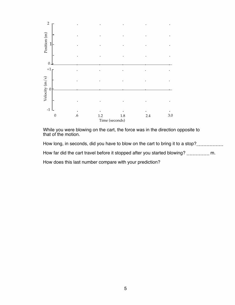
3. Sketch the position-time graph and the velocity-time graph and indicate thetime and position at which you started blowing on the cart, and the time andposition at which you stopped the cart. Also point out at which point on the graphthe cart started to change direction (if you could blow that long).

5

.6 1.2 1.8 2.4 3.00Time (seconds)

-1

+1

0

0

-

2

Posi

tion

(m)

Vel

ocity

(m/s

)

. . . . .-

. . . . .-

. . . . .-

. . . . .-

. . . . .-

1

. . . . .-

. . . . .-

. . . . .-

. . . . .-

. . . . .-

. . . . .-

While you were blowing on the cart, the force was in the direction opposite tothat of the motion.

How long, in seconds, did you have to blow on the cart to bring it to a stop? s.

How far did the cart travel before it stopped after you started blowing? m.

How does this last number compare with your prediction?


Physics 100 Lab: Forces in Equilibrium

Part 1: Forces in a straight line

IntroductionWe usually think that when a force is applied to an object, its motion changes.

But objects at rest may also have forces acting on them. For example, in a tug-of-warwhere both teams are equally matched, the forces on both ends of the rope are equaland the rope does not move. In this project, you will study forces which balance eachother, or are in equlibrium. You will also find the condition necessary for equilibrium.

What to doF1 = ________ F2 = ________

Get two similar spring scales. Hook both scales on the ring and gently pull on each inopposite directions as shown. Record the force exerted by each scale on the ring whichconnects them. (Use the N scale.)

Draw a force-vector diagram to scale.

Find the sum of the two forces F1 and F2 by adding the vectors tip to tail.

2

Place another spring scale parallel to one of the others as shown.Repeat the experiment measuring the three forces.

F1 = ________ F3 = ________

pullpull

pull

F2= ________

Draw a vector diagram showing F1, F2, and F3.

Find the vector sum of forces. What is the condition necessary for equilibrium?

Connect two springs in series to one side of the ring as shown. Balance their force withone spring on the other side. Measure the three forces.

pullpull

F1 = ________ F2= ________ F3 = ________

Explain the result you get. Why is it different from the parallel arrangement?

Part 2: 2 Dimensions

IntroductionIn order to analyse the forces in two dimensions one must record the angle of the

force as well as its magnitude. In the following exercises you will be given a paperprotractor to guide in applying the forces in specific directions or to help measure theangle of an arbitrary force. The condition for equilibrium for the two dimensional tug-of-war is very similar to that for one dimension. Can you see that the one dimensionalforce pull is a special case of the two dimensional one? Can you see how the twodimensional case can be generalized to three dimensions?

What to do

Push the center of the paper protractor on to the spindle

Place a metal ring on the center and pull outward on it with three similar spring scalesalong the directions of the grey lines.

As you pull the ring and keepit centered, read the forces onthe spring scales in N.

Draw vectors on the grey lineswhose lengths in tick marksequal the forces in N. Starteach vector at the center andpoint it outwards.

Add the vectors graphically toget the vector sum of theforces.

F1 = ________

F3 = ________

pull

pull

pull

F2= ________

You have two paper protractors on which the angles are marked with light grey lines.These are for the first two exercises. The third paper protractor has no lines on it. Pullalong any three directions you like on this one, draw the force vectors to scale, and findthe vector sum of forces.


5

Exercise 1: Forces at equal anglesInstructions:• Push the center of the paper protractor on to the spindle.• Place a metal ring on the center and pull outward on it with three spring scales along the directions of

the grey lines.• As you pull the ring, keep it centered, not touching the spindle. Read the force on the three scales in N.• Draw vectors on the grey lines whose lengths in tick marks represent the forces N. Start the tail of the

vectors at the center and point outwards.• Construct the vector sum of the three forces graphically on the paper.

9080

7060

50

40

3020

10

180 170160

150

140

130

120

110100

270

260

250

240

230

220

210

200190

350340

330

320

310

300

290

280

0


7

Exercise 2: Two forces at right angles

9080

7060

50

40

3020

10

180 170160

150

140

130

120

110100

270

260

250

240

230

220

210

200190

350340

330

320

310

300

290

280

0


9

Exercise 3: Forces at arbitrary angles

9080

7060

50

40

3020

10

180 170160

150

140

130

120

110100

270

260

250

240

230

220

210

200190

350340

330

320

310

300

290

280

0


Physics 100 Lab: Simple Harmonic MotionHarmonic motion occurs in many forms. Any system, which is slightly disturbed

from a stable equilibrium, will oscillate. When the force that restores the system toequilibrium is proportional to the displacement from equilibrium, the resultingoscillations follow Simple Harmonic Motion. Most oscillations in nature can beapproximated by simple harmonic motion. In today’s experiment you will study themotion of a cart, which is attached to two springs so that it rolls back and forth in a waythat is close to simple harmonic motion.

What to do

Open up the file L5#1 from the Lab#5 folder from the Physics 100 folder onthe desktop. This should display three graphs: position, velocity and acceleration. Thecart is tethered to the track by two springs and sits in equilibrium at about the middle ofthe track. Position the motion detector sensor about 1 m from the cart’s reflector and 17cm above the tabletop. The equilibrium position is now 1 m.

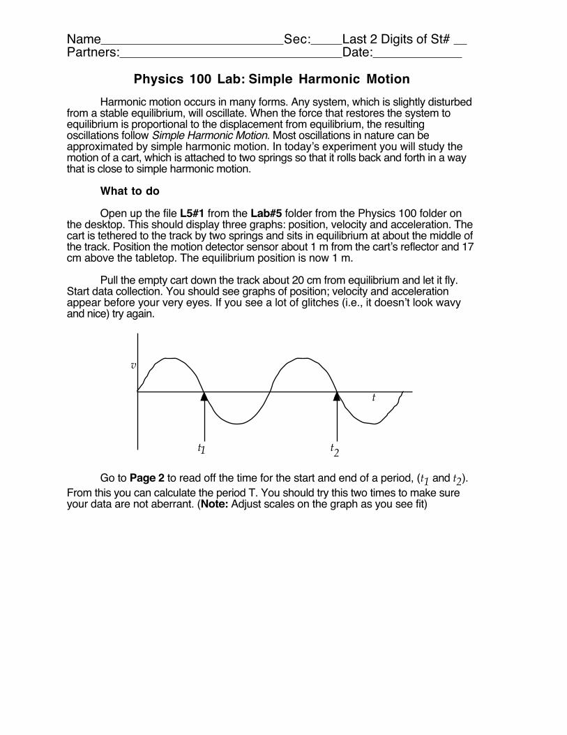
Pull the empty cart down the track about 20 cm from equilibrium and let it fly.Start data collection. You should see graphs of position; velocity and accelerationappear before your very eyes. If you see a lot of glitches (i.e., it doesn’t look wavyand nice) try again.

t t

v

t

1 2

Go to Page 2 to read off the time for the start and end of a period, (t1 and t2).From this you can calculate the period T. You should try this two times to make sureyour data are not aberrant. (Note: Adjust scales on the graph as you see fit)

–2–

Cart only: 0.5 kg

Time trial 1 trial 2(s)t1t2

T =t2 – t1

Now put two bars on the cart and repeat the experiment.

Cart with two masses: 1.5 kg

time trial 1 trial 2(s)t1t2

T =t2 – t1

Fill in the following table:

Mass Period, T(kg) (s)

m1 0.5m2 1.5

Is the period three time longer when the mass is three times more?________

Now try this: take the square root of the masses.

Mass Period, T(kg)1/2 (s)

m1 m2

m 1

m 2 =

T1T2

=

Does the period scale with the square root of the mass?

–3–

Does the period of the oscillation depend on the amplitude of vibration? In thefirst trials you pulled the cart back about 20 cm. The amplitude of the vibrationwas about 20 cm at first, and probably decreased a little as friction took its toll.

Try an amplitude of 10 cm, empty cart. What is the period?________

When the amplitude is 20 cm, empty cart, what is the period?________

Try an amplitude of 30 cm, empty cart. What is the period?________

Compare the empty-cart periods for initial amplitudes of 10, 20 and 30 cm.

You probably did find some small variation in the period. This variation may bewithin the accuracy of measurement, which is about 0.2 s. What other factorsmight account for the variation?

How could you use this apparatus to measure the masses of objects?

Could you use this method in a weightless environment? (Assume you canfind a way to keep the cart on the track.)

Is the mass you measure here the inertial mass or the gravitational mass?


Physics 100 Lab: Projectiles and Conservation of Energy

Caution:

•Wear Safety Glasses

•Don’t stick your finger into the Launcher. Use the plastic tube to loadthe ball.

Part 1: Projectiles

What to do

You can predict the trajectory of a ball fired from the projectile launcher. Place fourplastic hoops at evenly spaced positions along the trajectory so that the ballpasses through all the hoops after it is fired.

How to do it.

You already know enough to figure out where to place the hoops. Here are somesuggestions.

The launcher is clamped to the corner of your bench (see figure 1); it should beaimed such that the ball will hit the floor but not one of the benches. For thehorizontal launch the plumb bob should hang over the zero degree mark.

MINI LAUNCHER WEAR •SAFETY

DON

Figure 1: Horizontal launch

Place the steel ball in the barrel and push it down with the plastic pushrod until thetrigger catches the piston. DO NOT use your finger. Push the ball again until youhear another click; the launcher is now set at the medium range. Don't use the third(long range) setting. Now launch the ball by pulling on the string.

Tape a piece of paper on the floor where the ball hit the ground. Place apiece of carbon paper on top of the paper. Tape another piece of paper to the floordirectly below the launcher. Fire the ball again so that it marks the paper at the

–2–

point of impact. Use a plumb bob to find and mark the point on the floor that isdirectly below the release point on the barrel (this is marked by a cross at the sideof the launcher). Measure the horizontal distance the ball travels and the verticaldistance the ball drops. (Try it several times and take the average.)

Horizontal distance from launcher to point of impact on the floor: ____________

Measure the vertical distance from the launcher to the floor: ___________

Divide the horizontal distance into five equal intervals by finding four equallyspaced positions along the horizontal distance between the end of the launcherand the impact point. Fill in the horizontal positions in the table.

The ball travels across each horizontal interval in equal time. The ball drops underconstant acceleration during each interval. From the total distance it drops, figureout how far it will drop during each interval. Fill in the vertical drops in the table.

impact point

position 1 2 3 4launcher

Figure out how far the ball drops in each interval. Put the hoops there.

Figure 2: Trajectory of the ball

horizontal distance vertical droplauncher 0 m 0 m

position 1 ________ ________

position 2 ________ ________

position 3 ________ ________

position 4 ________ ________

impact (data from above) ________ _________

Measure the position for the first hoop. Place the hoop there, sticking it to theboard using velcro. Fire the launcher. If the ball misses make any adjustments andrecalculations as necessary.

After the first hoop is in place, continue with the second hoop and so on.

When all hoops are in the right place, sketch a scale drawing showing the hooppositions. Demonstrate to an instructor.

Calculate the horizontal launch velocity of the ball. vo =___________________

–3–

Part 2: Conservation of Energy

What to Do

Predict how high the ball would go when it is launched vertically, straight up.

Before we go on. Make a guess and write it here: Guessed hmax=

How to get it right

You can use the principle of energy conservation to predict the maximumheight of a ball launched straight up.• Assume the initial kinetic energy of the launched ball is the same in thevertical position as it is in the horizontal position.

• As the ball climbs up, its kinetic energy is converted into gravitationalpotential energy.

• The ball will be at its maximum height when all of the ball’s kinetic energy isconverted into increased gravitational potential energy of the ball.

1. Write the formula for the initial kinetic energy of the ball: KE0 =

2. Write the formula for the gravitational potential energy of the ball as a functionof its height. Let the PE at the launch position =0.

PEg =

3. Equate KE0 and PEg. Solve for hmax:

–4–

4. Calculate the value of hmax by using the last formula you derived. Assume thatthe mass of the ball is 0.0164 kg and use vo from part 1.

Predicted hmax=Now check it

Change the position of thelauncher to an inclination of 90°.Launch the ball and measure themaximum height reached by theball. One way to do this is to holda meter stick behind the launcherand mark the maximuim height onthe stick with tape. Repeat twomore times and average the threemeasurements.

90

initial position

final position

h

Figure 3: Vertical Launch

h1= h2= h2= hav=

ReflectQuestion Answer

(Circle one)

1. How good was your initial guess? Good Bad Ugly

2. How well did the measured value compare with thatwhich you predictedby calculation? Good Bad Ugly

3. If the mass of the ball were increased, how would themaximum height it reached be affected?

Higher Same Lower

4. At its maximum height the added potential energy comes from the kinetic energyof the ball at launch. Where did this kinetic energy come from?

5. What is the ball’s increase in gravitational potential energy in joules? J


Physics 100 Lab: EXPLOSIONS AND COLLISIONS

Two carts are pushed apart from rest as a result of a sudden force actingbetween them: an explosion. Two carts collide and bounce. Two carts collide andstick together. How does momentum help us understand what happens? You willfind the answer in this lab.

You have two carts:1) The dynamics cart (cart D) has a magnetic bumper on one side and a

Velcro™ sticker on the other. The Velcro™ side also has a spring-loaded plunger which can apply a sudden force after beingcompressed and released.

2) The collision cart (cart C) has Velcro™ stickers and magnetic bumperson both sides, but no spring-loaded plunger.

There are two metal bars for loading the carts with different masses. The track is furnished with a rubber bumper on one end and a c-clamp bumper on the other.

Activity 1: Two-cart explosions

You can measure the relative velocities of the two “exploding” cartswithout a computer. When one cart arrives at the end of the track before theother you hear two bumps. If the carts are released at the centre of the track andtravel with the same velocity they arrive at the same time and you hear onebump. The time from explosion to bumper impact is the same for both carts andwe will call it “one clunk”: ∆t = 1 clunk. If one cart moves faster, you can adjustthe starting position so the faster cart travels farther and they can be made toarrive at the same time. The velocities of the two carts are

v1 = ∆x1

∆t v2 =

∆x2

∆t where, for each cart, ∆x = xstop – xstart: its distance of travel from explosion tobumper. Assume the velocities remain essentially constant. Thus the velocity ofeach cart is proportional to the distance it travels and has units of m/clunk.

The momentum for each cart is got by multiplying the velocity by themass:

p1 = m1v1 = m1∆x1

∆t p2 = m2v2 = m2

∆x2

∆t .

Each cart and each metal bar have a mass of 0.5 kg.plunger

dynamicscart

collisioncart

∆x1 2x∆x

Fig: The position of the dynamics cart and the collision cartbefore the explosion and the distances each travels.

What to do

Fully compress and lock the spring plunger on the dynamics cart (cart D).To lock it, push it up slightly after compressing it so the slot in the rod catches onthe metal edge at the top of the hole. Place cart D near the middle of the track.Place the collision cart (cart C) next to the plunger side of cart D so the spring willpush against the second cart and the Velcro™ buttons stick to each other.

Release the spring by gently tapping on the release rod with the edge ofthe wooden block. (Using the block helps prevent accidentally giving the cart ahorizontal push).

With the carts unloaded, find the explosion position which results in bothcarts reaching the track’s end at the same time. Try to find the starting position tothe nearest cm. You can mark the outside edge of one cart (its xstart) using theslider on the track. The xstart of the other cart is 34 cm away. Calculate themomentum of each cart after the explosion in units of "kg-m/clunk".

unloaded m xstop xstart ∆x momentumcart (kg) (m) (m) (m) (kg·m/clunk)

cart C 0.5 0.015cart D 0.5 1.200

total p —>

•Compare total momentum of the carts after the explosion to the total momentumbefore.

• Does the movement depend on which cart had the plunger in it?

Put one metal bar on the dynamics cart, find the starting position thatgives one bump and calculate the momentum.

one cart m xstop xstart ∆x momentumloaded (kg) (m) (m) (m) (kg·m/clunk)cart C 0.5 0.015cart D 1.0 1.200

total p —>

–2–

Prediction: If you were to put another 0.5 kg mass on the dynamics cart, predictwhere you would have to start for one bump. Fill in the xstart cells and then try it.

one cartreally

m xstop xstartpredicted

∆xpredicted

momentum

loaded (kg) (m) (m) (m) (kg·m/clunk)cart C 0.5 0.015cart D 1.5 1.200

total p —>

Activity 2: Elastic Collisions (“bump and run”)

The collisions in this activity are elastic, because all the kinetic energy dueto movement of the carts returns to the carts after the collision. The conversion ofkinetic energy to potential energy during the collision is temporary.

What to do

Remove all the bricks from the carts. Turn the dynamics cart (cart D)around so that its magnetic bumper aligns with the magnetic bumper of thecollision cart (cart C). Place cart D in the middle of the track and give cart C agentle but firm shove towards it in the positive* direction and let them collide.

Elastic collision, both cartshaving equal masses

largenegative*

smallnegative

zero smallpositive

largepositive

velocity of cart C before collisionvelocity of cart D before collision Xvelocity of cart C after collisionvelocity of cart D after collision*Positive means towards the high end of the cm scale, negative towards the 0 cm end.

Put a mass bar in cart C. Repeat the collision and fill in the next table.

Elastic collision, hitter moremassive than hittee

largenegative

smallnegative

zero smallpositive

largepositive

velocity of cart C before collisionvelocity of cart D before collision Xvelocity of cart C after collisionvelocity of cart D after collision

–3–

Remove the mass bar from cart C and put it in cart D. Repeat the collisionand fill in the table.

Elastic collision, hittee moremassive than hitter

largenegative

smallnegative

zero smallpositive

largepositive

velocity of cart C before collisionvelocity of cart D before collision Xvelocity of cart C after collisionvelocity of cart D after collision

• Explain the differences in the three collisions using momentum conservation.

Activity 3: Inelastic Collisions ("Hit and Stick")

If you turn the dynamics cart around so that the collision cart sticks to theVelcro™ then some of the kinetic energy is permanently lost to other forms ofenergy. Collisions where kinetic energy is lost are called inelastic collisions.

What to doRepeat the collisions of the last section giving the collision cart about the

same initial velocity each time. Record the relative velocities of the combinedcarts after the collision

Inelastic collisions Velocity of combined carts after the collision.

zero small medium largemC < mDmC = mDmC > mD

•Explain the differences in the three collisions using momentum conservation.

If you have time, set up the ultrasonic motion detector to measure the velocities of the collisioncart before and after the inelastic collisions. (21 cm above the track, 40 cm from its end.) Recordthe velocities of the collision cart immediately before and after the inelastic collision. Ismomentum conserved during each collision? What happens to the kinetic energy?

velocity of cart Cbefore collision

velocity of cartsafter collision

Total momentumbefore collision

Total momentumafter collision

mC < mDmC = mDmC > mD

–4–


Physics 100 Lab: Electrified Objects

When objects are rubbed they acquire a net electrical charge. All materialconsists of charged particles, but usually these charges are balanced so the material issaid to be “uncharged” or neutral. Rubbing causes a small number of charges to betransferred from one material to another—the objects become “charged.” While theexact mechanism of charge transfer is still not fully understood, the earliest qualitativeelectricity experiments using this effect occurred in the 18th century. Transfer ofcharged by rubbing is called called “triboelectricity.” Giving something we don’tunderstand a fancy name makes us feel better.

You can observe for yourself the behaviour of electric charges by rubbing plasticstrips with paper or cloth. The ease of doing these experiments varies with atmospherichumidity because moisture adsorbed on surfaces allows charge to leak away. So if it’s awarm, rainy day, be patient.

What to do

Two pieces of plastic hang from a ring stand: The clear strip is cellulose acetateand the white strip is Vinylite. Briskly rub each suspended piece of plastic with drypaper. Do not touch the rubbed surfaces. Rub another Vinylite strip with paper and bringit near each of the suspended strips.

• What happens?:

Rub another strip of acetate with paper and bring it near the hanging strips.

• What happens?:

• Have you found one, two or three kinds of charge?

• Assign names to each kind of charge you have found and use these names inthe next exercise.

Rub some other objects. Hold them close to the charged plastic strips anddiscover what kind of charge they have. Try rubbing a plastic ruler, comb or balloon onyour clothes. Try pulling apart two pieces of cellophane tape which were stuck togethersticky-side-to-back-side. How are the surfaces charged after you pull them apart?

The original definition of positive charge was the charge acquired by a glass rod whenrubbed by silk. Borrow the glass rod and silk and use it to identify the charges on thevinyl and acetate in terms of conventional terminology.

Attracting an uncharged metal ball

+ +++++

––––

A small graphite coated ball hangs from an insulatingthread. When you touch it you allow any excess chargeson it to flow away through your body. This process iscalled “grounding.” Touch the ball momentarily to ensurethat it is uncharged. Rub a piece of acetate and slowlybring it close to the metal ball.

What happens when the charged plastic strip comes near the ball?

What happens when the ball touches the charged strip? Why?

Touch the ball with your hand to discharge it and repeat the above experiment withVinylite. Describe any differences or similarities.

Inducing charge

Place an aluminum rod on a beakerand put one end of the rod within 1 mm ofthe hanging metal ball. Touch the rod andball to make sure they are discharged.Rub an acetate strip and bring it close tothe aluminum rod. Try to get as close aspossible but don’t touch the rod.

• Explain what happens to the ball bydrawing the charges on the aluminumrod and on the ball. –––>

Replace the aluminum rod with aplastic rod and try to make the ball move.

+ ++

Pyrex

Aluminum Rod

–2–

Electric Ping Pong.

Hang the metal ball mid-way between two aluminumrods with a few mm clear-ance between the ball andeach rod. Touch all the metalobjects to discharge them.Rub an acetate strip, bring itclose to the end of one of themetal rods as you did before.Hold it there for about 15seconds and watch the metalball.

Take the charged plasticstrip away from the metal rodand keep watching the ball.

Pyrex

Aluminum Rod

Can you explain what you see? Describe briefly what happened and try to explain it bydrawing cartoons on the last page.

Party tricks*

Take some good tape, like electrical tape, into a very dark room. After your eyeshave adapted to the dark, quickly pull a length of it off the roll while you and your friendsare looking at it. You will see a bright flash caused by electrical sparks flashing as thesurfaces get charged.

Also while in the dark room, crush a wintergreen lifesaver between the jaws of pliers.Bright flashes will amaze your friends. Do you still get bright flashes when you chompon one with your teeth? What about other flavours? Try it!

* Did you ever learn party tricks in a Biology or Chemistry lab?

–3–

Pyrex

++++

1 2

3 4

5 6

–4–


Physics 100 Lab: REFLECTION AND REFRACTION

Many properties of light can be modelled by rays emerging from a lightsource, hitting an object and entering your eye. Optical devices can beunderstood by learning how lenses and mirrors change the paths of the rays inorder to magnify, reduce or change the positions of images.

Straight line ray propagation

How can you show that light travels in a straight line? Put three pins in astraight line and sight down them. If the light reflected from the far pin passes themiddle one and the near one before entering your eye then the pins will appear tobe on top of each other.

Put three pins on the circularray protractor supplied. Put one in thecentre of the circle and two at the two0° points. Are the pins in a straightline? When you sight down them withone eye can you move your head untilthey all appear on top of each other?Are you absolutely convinced that lighttravels in a straight line in thissituation?

lightsource

pin

pin

pin

eye

light "rays"

1

0°

0°

Reflection

When you look at an image of a pin in a mirror, you have no way ofknowing where the light rays reaching your eye hit the mirror. If there is a scratchon the mirror and you move your head so that the image is lined up with thescratch then you know that the incident ray hits the mirror at the scratch.

pin

pin

mirror

silveredsurface scratch

90° angle

2

90° 90°

0°

0°

pin 2 30°pin 1

3

Remove the centre pin. Place the mirror with its scratch over the circle's centrepoint and its back on the 90°–90° line .If you sight down the pin towards the scratch you should see

1. the near pin,2. the image of near pin in the mirror,3. the far pin over the top of the mirror and4. the scratch on the back of the mirror.

All four should appear on top of each other. If not then the mirror is probably notplaced exactly right. Once this alignment is attained don't move themirror while you do the next step.

Remove pin 1 and place it at the 30° mark. Sight from pin 1 to the scratch on themirror and place pin 2 so its image in the mirror appears in line with the scratchand with pin 1. Make sure pin 1, the image of pin 2 and the scratch all look likethey are on top of each other.

Now a light ray from pin 2 strikes the mirror at the scratch and reflects back intoyour eye.

What is the angle of incidence? What is the angle of reflection?

Reverse the procedure. Place pin 2 at some other angle (in front of the mirror)and find the position of pin 1 that aligns the pins and the scratch when you sightthrough pin 1 towards the scratch.

What is the angle of incidence? What is the angle of reflection?

In both cases angles of incidence and reflection should agree within theaccuracy of your pin-sticking.

Have your partner stick a pin at a third location. Predict where you would haveto stick the other pin so they appear aligned and then put the pin there and

–2–

check. Sight from both pin 1 towards the scratch and from pin 2 towards thescratch, in other words, check the reversibility of the ray’s path.

Did you succeed in predicting the correct position? Of course.Is the ray’s path reversible? .

Refraction

There’s a semicircular Lucite™ block which you can use to explore howlight is refracted. Put the flat face of the Lucite™ block on the ray protractorcentred on the 90°–90° line . The vertical line in the middle of the flat faceshould lie on top of the protractor’s centre point. Stick pins in both 0° marks andsight along them through the plastic block. You should see both pins and theline on top of each other because the light ray from the pin passes through fromair to plastic and from plastic to air at a 90° angle to the surfaces.

Move the near pin (pin 1) to the 10° point.Sighting along pin 1 to the line on the plastic andlook through the plastic block find the position ofpin 2 where both pins and the line appear on topof each other. Notice that the ray from pin 2 willalways hit the curved side of the plastic block atright angles. The angle of the ray in air withrespect to the normal to the surface is theposition of pin 1 on the circle and the angle of theray inside the plastic is given by the position ofpin 2 on the circle. This angle would be the sameif the plastic block were bigger than the protractorand the pin were inside the plastic.

pin 2

pin 1

90° angle

A

B

C

F

E

D

The length of the semicords DF and AC can be read from the linear scale on theray protractor. This length of the semicords in decimetres is equal to the sines ofthe angles. Make readings at angles shown in the table.

angle in air (pin 1)

angle in plastic(pin 2)

length of semicordAC (dm)

length of semicordDF (dm)

0° 0° 0 010°20°40°60°80°

Plot the six angles in plastic vs. the six angles in air on the next page. Then plotthe sines of the angles.

–3–

angle in air

0° 10° 20° 30° 40° 50° 60° 70° 80° 90°

90°

80°

70°

60°

50°

40°

30°

20°

10°

0°

angl

e in

pla

stic

Estimate the index ofrefraction by calcu-lating 1/slope of thegraph at small an-gles.

Estimate what inci-dent angle (θc) inplastic would give a90° angle in air.

What would happento the ray in air if theray in plastic wereincident at an anglegreater than θc?

sine of angle in air

0 0.1 0.2 0.3 0.4 0.5 0.6 0.7 0.8 0.9

0.9

0.8

0.7

0.6

0.5

0.4

0.3

0.2

0.1

0

sine

of a

ngle

in p

last

ic

1

1

Does this graph ofthe sines of theangles appearlinear throughoutthe entire range ofobservation?

What index of re-fraction do you getfrom this graph?

–4–

9080

7060

50

40

3020

10

0 1020

30

40

50

6070

8090

8070

60

50

40

3020

10

1020

30

40

50

6070

80

0

.1 0.2.3.4.5.6.7.8.91 .1 .2 .3 .4 .5 .6 .7 .8 .9 1

.10 .2 .3 .4 .5 .6 .7 .8 .9 1.1.2.3.4.5.6.7.8.91

physics 100 lab 1: introduction to motion - sfu.camxchen/phys100/p100labs.pdf · page 1-2 real time...

Documents