physical review d all-sky search for periodic ...tanner/pdfs/abbott08prd-all-sky-periodic.pdf ·...

All-sky search for periodic gravitational waves in LIGO S4 data

B. Abbott,15 R. Abbott,15 R. Adhikari,15 J. Agresti,15 P. Ajith,2 B. Allen,2,50 R. Amin,19 S. B. Anderson,15

W. G. Anderson,50 M. Arain,39 M. Araya,15 H. Armandula,15 M. Ashley,4 S. Aston,38 P. Aufmuth,14 C. Aulbert,1 S. Babak,1

S. Ballmer,15 H. Bantilan,8 B. C. Barish,15 C. Barker,16 D. Barker,16 B. Barr,40 P. Barriga,49 M. A. Barton,40 K. Bayer,18

K. Belczynski,25 J. Betzwieser,18 P. T. Beyersdorf,28 B. Bhawal,15 I. A. Bilenko,22 G. Billingsley,15 R. Biswas,50

E. Black,15 K. Blackburn,15 L. Blackburn,18 D. Blair,49 B. Bland,16 J. Bogenstahl,40 L. Bogue,17 R. Bork,15 V. Boschi,15

S. Bose,51 P. R. Brady,50 V. B. Braginsky,22 J. E. Brau,43 M. Brinkmann,2 A. Brooks,37 D. A. Brown,15,6 A. Bullington,31

A. Bunkowski,2 A. Buonanno,41 O. Burmeister,2 D. Busby,15 R. L. Byer,31 L. Cadonati,18 G. Cagnoli,40 J. B. Camp,23

J. Cannizzo,23 K. Cannon,50 C. A. Cantley,40 J. Cao,18 L. Cardenas,15 M. M. Casey,40 G. Castaldi,46 C. Cepeda,15

E. Chalkley,40 P. Charlton,9 S. Chatterji,15 S. Chelkowski,2 Y. Chen,1 F. Chiadini,45 D. Chin,42 E. Chin,49 J. Chow,4

N. Christensen,8 J. Clark,40 P. Cochrane,2 T. Cokelaer,7 C. N. Colacino,38 R. Coldwell,39 R. Conte,45 D. Cook,16

T. Corbitt,18 D. Coward,49 D. Coyne,15 J. D. E. Creighton,50 T. D. Creighton,15 R. P. Croce,46 D. R. M. Crooks,40

A. M. Cruise,38 A. Cumming,40 J. Dalrymple,32 E. D’Ambrosio,15 K. Danzmann,14,2 G. Davies,7 D. DeBra,31

J. Degallaix,49 M. Degree,31 T. Demma,46 V. Dergachev,42 S. Desai,33 R. DeSalvo,15 S. Dhurandhar,13 M. Dıaz,34

J. Dickson,4 A. Di Credico,32 G. Diederichs,14 A. Dietz,7 E. E. Doomes,30 R. W. P. Drever,5 J.-C. Dumas,49 R. J. Dupuis,15

J. G. Dwyer,10 P. Ehrens,15 E. Espinoza,15 T. Etzel,15 M. Evans,15 T. Evans,17 S. Fairhurst,7,15 Y. Fan,49 D. Fazi,15

M. M. Fejer,31 L. S. Finn,33 V. Fiumara,45 N. Fotopoulos,50 A. Franzen,14 K. Y. Franzen,39 A. Freise,38 R. Frey,43

T. Fricke,44 P. Fritschel,18 V. V. Frolov,17 M. Fyffe,17 V. Galdi,46 J. Garofoli,16 I. Gholami,1 J. A. Giaime,17,19

S. Giampanis,44 K. D. Giardina,17 K. Goda,18 E. Goetz,42 L. M. Goggin,15 G. Gonzalez,19 S. Gossler,4 A. Grant,40

S. Gras,49 C. Gray,16 M. Gray,4 J. Greenhalgh,27 A. M. Gretarsson,11 R. Grosso,34 H. Grote,2 S. Grunewald,1

M. Guenther,16 R. Gustafson,42 B. Hage,14 D. Hammer,50 C. Hanna,19 J. Hanson,17 J. Harms,2 G. Harry,18 E. Harstad,43

T. Hayler,27 J. Heefner,15 I. S. Heng,40 A. Heptonstall,40 M. Heurs,2 M. Hewitson,2 S. Hild,14 E. Hirose,32 D. Hoak,17

D. Hosken,37 J. Hough,40 E. Howell,49 D. Hoyland,38 S. H. Huttner,40 D. Ingram,16 E. Innerhofer,18 M. Ito,43 Y. Itoh,50

A. Ivanov,15 D. Jackrel,31 B. Johnson,16 W. W. Johnson,19 D. I. Jones,47 G. Jones,7 R. Jones,40 L. Ju,49 P. Kalmus,10

V. Kalogera,25 D. Kasprzyk,38 E. Katsavounidis,18 K. Kawabe,16 S. Kawamura,24 F. Kawazoe,24 W. Kells,15

D. G. Keppel,15 F. Ya. Khalili,22 C. Kim,25 P. King,15 J. S. Kissel,19 S. Klimenko,39 K. Kokeyama,24 V. Kondrashov,15

R. K. Kopparapu,19 D. Kozak,15 B. Krishnan,1 P. Kwee,14 P. K. Lam,4 M. Landry,16 B. Lantz,31 A. Lazzarini,15 B. Lee,49

M. Lei,15 J. Leiner,51 V. Leonhardt,24 I. Leonor,43 K. Libbrecht,15 P. Lindquist,15 N. A. Lockerbie,48 M. Longo,45

M. Lormand,17 M. Lubinski,16 H. Luck,14,2 B. Machenschalk,1 M. MacInnis,18 M. Mageswaran,15 K. Mailand,15

M. Malec,14 V. Mandic,15 S. Marano,45 S. Marka,10 J. Markowitz,18 E. Maros,15 I. Martin,40 J. N. Marx,15 K. Mason,18

L. Matone,10 V. Matta,45 N. Mavalvala,18 R. McCarthy,16 D. E. McClelland,4 S. C. McGuire,30 M. McHugh,21

K. McKenzie,4 J. W. C. McNabb,33 S. McWilliams,23 T. Meier,14 A. Melissinos,44 G. Mendell,16 R. A. Mercer,39

S. Meshkov,15 C. J. Messenger,40 D. Meyers,15 E. Mikhailov,18 S. Mitra,13 V. P. Mitrofanov,22 G. Mitselmakher,39

R. Mittleman,18 O. Miyakawa,15 S. Mohanty,34 G. Moreno,16 K. Mossavi,2 C. MowLowry,4 A. Moylan,4 D. Mudge,37

G. Mueller,39 S. Mukherjee,34 H. Muller-Ebhardt,2 J. Munch,37 P. Murray,40 E. Myers,16 J. Myers,16 T. Nash,15

G. Newton,40 A. Nishizawa,24 K. Numata,23 B. O’Reilly,17 R. O’Shaughnessy,25 D. J. Ottaway,18 H. Overmier,17

B. J. Owen,33 Y. Pan,41 M. A. Papa,1,50 V. Parameshwaraiah,16 P. Patel,15 M. Pedraza,15 S. Penn,12 V. Pierro,46 I. M. Pinto,46

M. Pitkin,40 H. Pletsch,2 M. V. Plissi,40 F. Postiglione,45 R. Prix,1 V. Quetschke,39 F. Raab,16 D. Rabeling,4 H. Radkins,16

R. Rahkola,43 N. Rainer,2 M. Rakhmanov,33 M. Ramsunder,33 K. Rawlins,18 S. Ray-Majumder,50 V. Re,38 H. Rehbein,2

S. Reid,40 D. H. Reitze,39 L. Ribichini,2 R. Riesen,17 K. Riles,42 B. Rivera,16 N. A. Robertson,15,40 C. Robinson,7

E. L. Robinson,38 S. Roddy,17 A. Rodriguez,19 A. M. Rogan,51 J. Rollins,10 J. D. Romano,7 J. Romie,17 R. Route,31

S. Rowan,40 A. Rudiger,2 L. Ruet,18 P. Russell,15 K. Ryan,16 S. Sakata,24 M. Samidi,15 L. Sancho de la Jordana,36

V. Sandberg,16 V. Sannibale,15 S. Saraf,26 P. Sarin,18 B. S. Sathyaprakash,7 S. Sato,24 P. R. Saulson,32 R. Savage,16

P. Savov,6 S. Schediwy,49 R. Schilling,2 R. Schnabel,2 R. Schofield,43 B. F. Schutz,1,7 P. Schwinberg,16 S. M. Scott,4

A. C. Searle,4 B. Sears,15 F. Seifert,2 D. Sellers,17 A. S. Sengupta,7 P. Shawhan,41 D. H. Shoemaker,18 A. Sibley,17

X. Siemens,15,6 D. Sigg,16 S. Sinha,31 A. M. Sintes,36,1 B. J. J. Slagmolen,4 J. Slutsky,19 J. R. Smith,2 M. R. Smith,15

K. Somiya,2,1 K. A. Strain,40 D. M. Strom,43 A. Stuver,33 T. Z. Summerscales,3 K.-X. Sun,31 M. Sung,19 P. J. Sutton,15

H. Takahashi,1 D. B. Tanner,39 M. Tarallo,15 R. Taylor,15 R. Taylor,40 J. Thacker,17 K. A. Thorne,33 K. S. Thorne,6

A. Thuring,14 K. V. Tokmakov,40 C. Torres,34 C. Torrie,40 G. Traylor,17 M. Trias,36 W. Tyler,15 D. Ugolini,35 C. Ungarelli,38

K. Urbanek,31 H. Vahlbruch,14 M. Vallisneri,6 C. Van Den Broeck,7 M. Varvella,15 S. Vass,15 A. Vecchio,38 J. Veitch,40

PHYSICAL REVIEW D 77, 022001 (2008)

1550-7998=2008=77(2)=022001(38) 022001-1 © 2008 The American Physical Society

P. Veitch,37 A. Villar,15 C. Vorvick,16 S. P. Vyachanin,22 S. J. Waldman,15 L. Wallace,15 H. Ward,40 R. Ward,15 K. Watts,17

D. Webber,15 A. Weidner,2 M. Weinert,2 A. Weinstein,15 R. Weiss,18 S. Wen,19 K. Wette,4 J. T. Whelan,1 D. M. Whitbeck,33

S. E. Whitcomb,15 B. F. Whiting,39 C. Wilkinson,16 P. A. Willems,15 L. Williams,39 B. Willke,14,2 I. Wilmut,27

W. Winkler,2 C. C. Wipf,18 S. Wise,39 A. G. Wiseman,50 G. Woan,40 D. Woods,50 R. Wooley,17 J. Worden,16 W. Wu,39

I. Yakushin,17 H. Yamamoto,15 Z. Yan,49 S. Yoshida,29 N. Yunes,33 M. Zanolin,18 J. Zhang,42 L. Zhang,15 C. Zhao,49

N. Zotov,20 M. Zucker,18 H. zur Muhlen,14 and J. Zweizig15

(LIGO Scientific Collaboration)

1Albert-Einstein-Institut, Max-Planck-Institut fur Gravitationsphysik, D-14476 Golm, Germany2Albert-Einstein-Institut, Max-Planck-Institut fur Gravitationsphysik, D-30167 Hannover, Germany

3Andrews University, Berrien Springs, Michigan 49104 USA4Australian National University, Canberra, 0200, Australia

5California Institute of Technology, Pasadena, California 91125, USA6Caltech-CaRT, Pasadena, California 91125, USA

7Cardiff University, Cardiff, CF24 3AA, United Kingdom8Carleton College, Northfield, Minnesota 55057, USA

9Charles Sturt University, Wagga Wagga, NSW 2678, Australia10Columbia University, New York, New York 10027, USA

11Embry-Riddle Aeronautical University, Prescott, Arizona 86301 USA12Hobart and William Smith Colleges, Geneva, New York 14456, USA

13Inter-University Centre for Astronomy and Astrophysics, Pune - 411007, India14Leibnitz Universitat Hannover, D-30167 Hannover, Germany

15LIGO - California Institute of Technology, Pasadena, California 91125, USA16LIGO Hanford Observatory, Richland, Washington 99352, USA

17LIGO Livingston Observatory, Livingston, Louisiana 70754, USA18LIGO - Massachusetts Institute of Technology, Cambridge, Massachusetts 02139, USA

19Louisiana State University, Baton Rouge, Louisiana 70803, USA20Louisiana Tech University, Ruston, Louisiana 71272, USA

21Loyola University, New Orleans, Louisiana 70118, USA22Moscow State University, Moscow, 119992, Russia

23NASA/Goddard Space Flight Center, Greenbelt, Maryland 20771, USA24National Astronomical Observatory of Japan, Tokyo 181-8588, Japan

25Northwestern University, Evanston, Illinois 60208, USA26Rochester Institute of Technology, Rochester, New York 14623, USA

27Rutherford Appleton Laboratory, Chilton, Didcot, Oxon OX11 0QX United Kingdom28San Jose State University, San Jose, California 95192, USA

29Southeastern Louisiana University, Hammond, Louisiana 70402, USA30Southern University and A&M College, Baton Rouge, Louisiana 70813, USA

31Stanford University, Stanford, California 94305, USA32Syracuse University, Syracuse, New York 13244, USA

33The Pennsylvania State University, University Park, Pennsylvania 16802, USA34The University of Texas at Brownsville and Texas Southmost College, Brownsville, Texas 78520, USA

35Trinity University, San Antonio, Texas 78212, USA36Universitat de les Illes Balears, E-07122 Palma de Mallorca, Spain

37University of Adelaide, Adelaide, SA 5005, Australia38University of Birmingham, Birmingham, B15 2TT, United Kingdom

39University of Florida, Gainesville, Florida 32611, USA40University of Glasgow, Glasgow, G12 8QQ, United Kingdom41University of Maryland, College Park, Maryland 20742 USA

42University of Michigan, Ann Arbor, Michigan 48109, USA43University of Oregon, Eugene, Oregon 97403, USA

44University of Rochester, Rochester, New York 14627, USA45University of Salerno, 84084 Fisciano (Salerno), Italy

46University of Sannio at Benevento, I-82100 Benevento, Italy47University of Southampton, Southampton, SO17 1BJ, United Kingdom

48University of Strathclyde, Glasgow, G1 1XQ, United Kingdom49University of Western Australia, Crawley, Washington 6009, Australia, USA

50University of Wisconsin-Milwaukee, Milwaukee, Wisconsin 53201, USA

B. ABBOTT et al. PHYSICAL REVIEW D 77, 022001 (2008)

022001-2

51Washington State University, Pullman, Washington 99164, USA(Received 11 September 2007; published 10 January 2008)

We report on an all-sky search with the LIGO detectors for periodic gravitational waves in thefrequency range 50–1000 Hz and with the frequency’s time derivative in the range �1� 10�8 Hz s�1 tozero. Data from the fourth LIGO science run (S4) have been used in this search. Three differentsemicoherent methods of transforming and summing strain power from short Fourier transforms(SFTs) of the calibrated data have been used. The first, known as StackSlide, averages normalized powerfrom each SFT. A ‘‘weighted Hough’’ scheme is also developed and used, which also allows for a multi-interferometer search. The third method, known as PowerFlux, is a variant of the StackSlide method inwhich the power is weighted before summing. In both the weighted Hough and PowerFlux methods, theweights are chosen according to the noise and detector antenna-pattern to maximize the signal-to-noiseratio. The respective advantages and disadvantages of these methods are discussed. Observing no evidenceof periodic gravitational radiation, we report upper limits; we interpret these as limits on this radiationfrom isolated rotating neutron stars. The best population-based upper limit with 95% confidence on thegravitational-wave strain amplitude, found for simulated sources distributed isotropically across the skyand with isotropically distributed spin axes, is 4:28� 10�24 (near 140 Hz). Strict upper limits are alsoobtained for small patches on the sky for best-case and worst-case inclinations of the spin axes.

DOI: 10.1103/PhysRevD.77.022001 PACS numbers: 04.80.Nn, 07.05.Kf, 95.55.Ym, 97.60.Gb

I. INTRODUCTION

We report on a search with the LIGO (LaserInterferometer Gravitational-wave Observatory) detectors[1,2] for periodic gravitational waves in the frequencyrange 50–1000 Hz and with the frequency’s time derivativein the range �1� 10�8 Hz s�1 to zero. The search iscarried out over the entire sky using data from the fourthLIGO science run (S4). Isolated rotating neutron stars inour galaxy are the prime target.

Using data from earlier science runs, the LIGOScientific Collaboration (LSC) has previously reported onsearches for periodic gravitational radiation, using a long-period coherent method to target known pulsars [3–5],using a short-period coherent method to target ScorpiusX-1 in selected bands and search the entire sky in the160.0–728.8 Hz band [6], and using a long-period semi-coherent method to search the entire sky in the 200–400 Hz band [7]. Einstein@Home, a distributed homecomputing effort running under the BOINC architecture[8], has also been searching the entire sky using a coherentfirst stage, followed by a simple coincidence stage [9]. Incomparison, this paper: (1) examines more sensitive data;(2) searches over a larger range in frequency and itsderivative; and (3) uses three alternative semicoherentmethods for summing measured strain powers to detectexcess power from a continuous gravitational-wave signal.

The first purpose of this paper is to present results fromour search for periodic gravitational waves in the S4 data.Over the LIGO frequency band of sensitivity, the S4 all-skyupper limits presented here are approximately an order ofmagnitude better than published previously from earlierscience runs [6,7]. After following up on outliers in thedata, we find that no candidates survive, and thus reportupper limits. These are interpreted as limits on radiationfrom rotating neutron stars, which can be expressed as

functions of the star’s ellipticity and distance, allowingfor an astrophysical interpretation. The best population-based upper limit with 95% confidence on thegravitational-wave strain amplitude, found for simulatedsources distributed isotropically across the sky and withisotropically distributed spin axes, is 4:28� 10�24 (near140 Hz). Strict upper limits are also obtained for smallpatches on the sky for best-case and worst-case inclinationsof the spin axes.

The second purpose of this paper, along with the pre-vious coherent [6] and semicoherent [7] papers, is to laythe foundation for the methods that will be used in futuresearches. It is well known that the search for periodicgravitational waves is computationally bound; to obtainoptimal results will require a hierarchical approach thatuses coherent and semicoherent stages [10–13]. A fifthscience run (S5), which started in November 2005, isgenerating data at initial LIGO’s design sensitivity. Weplan to search this data using the best methods possible,based on what is learned from this and previous analyses.

In the three methods considered here, one searches forcumulative excess power from a hypothetical periodicgravitational-wave signal by examining successive spectralestimates based on short Fourier transforms (SFTs) of thecalibrated detector strain data channel, taking into accountthe Doppler modulations of detected frequency due to theEarth’s rotational and orbital motion with respect to thesolar system barycenter (SSB), and the time derivative ofthe frequency intrinsic to the source. The simplest methodpresented, known as ‘‘StackSlide’’ [12–15], averages nor-malized power from each SFT. In the Hough methodreported previously [7,10], referred to here as ‘‘standardHough,’’ the sum is of binary zeroes or ones, where a SFTcontributes unity if the power exceeds a normalized powerthreshold. In this paper a ‘‘weighted Hough’’ scheme,

ALL-SKY SEARCH FOR PERIODIC GRAVITATIONAL . . . PHYSICAL REVIEW D 77, 022001 (2008)

022001-3

http://dx.doi.org/10.1103/PhysRevD.77.022001

henceforth also referred to as ‘‘Hough,’’ has been devel-oped and is similar to that described in Ref. [16]. Thisscheme also allows for a multi-interferometer search. Thethird method, known as ‘‘PowerFlux’’ [17], is a variant ofthe StackSlide method in which the power is weightedbefore summing. In both the weighted Hough andPowerFlux methods, the weights are chosen according tothe noise and detector antenna pattern to maximize thesignal-to-noise ratio.

The Hough method is computationally faster and morerobust against large transient power artifacts, but is slightlyless sensitive than StackSlide for stationary data [7,15].The PowerFlux method is found in most frequency rangesto have better detection efficiency than the StackSlide andHough methods, the exceptions occurring in bands withlarge nonstationary artifacts, for which the Hough methodproves more robust. However, the StackSlide and Houghmethods can be made more sensitive by starting with themaximum likelihood statistic (known as the F -statistic[6,10,18]) rather than SFT power as the input data, thoughthis improvement comes with increased computationalcost. The trade-offs among the methods mean that eachcould play a role in our future searches.

In brief, this paper makes several important contribu-tions. It sets the best all-sky upper limits on periodicgravitational waves to date, and shows that these limitsare becoming astrophysically interesting. It also introducesmethods that are crucial to the development of our futuresearches.

This paper is organized as follows: Sec. II briefly de-scribes the LIGO interferometers, focusing on improve-ments made for the S4 data run, and discusses thesensitivity and relevant detector artifacts. Section III pre-cisely defines the waveforms we seek and the associatedassumptions we have made. Section IV gives a detaileddescription of the three analysis methods used and sum-marizes their similarities and differences, while Sec. Vgives the details of their implementations and the pipelinesused. Section VI discusses the validation of the softwareand, as an end-to-end test, shows the detection of simulatedpulsar signals injected into the data stream at the hardwarelevel. Section VII describes the search results, andSec. VIII compares the results from the three respectivemethods. Section IX concludes with a summary of theresults, their astrophysical implications, and future plans.

II. THE LIGO DETECTOR NETWORKAND THE S4 SCIENCE RUN

The LIGO detector network consists of a 4-km interfer-ometer in Livingston, Louisiana (called L1) and two inter-ferometers in Hanford, Washington, one 4-km and another2-km (H1 and H2, respectively).

The data analyzed in this paper were produced duringLIGO’s 29.5-day fourth science run (S4) [19]. This runstarted at noon Central Standard Time (CST) on February

22 and ended at midnight CST on March 23, 2005. Duringthe run, all three LIGO detectors had displacementspectral amplitudes near 2:5� 10�19 m Hz�1=2 in theirmost sensitive frequency band near 150 Hz. In units ofgravitational-wave strain amplitude, the sensitivity of H2 isroughly a factor of 2 worse than that of H1 and L1 overmuch of the search band. The typical strain sensitivities inthis run were within a factor of 2 of the design goals.Figure 1 shows representative strain spectral noise den-sities for the three interferometers during the run. Asdiscussed in Sec. V below, however, nonstationarity ofthe noise was significant.

Changes to the interferometers before the S4 run in-cluded the following improvements [19]:

(i) Installation of active seismic isolation of supportstructures at Livingston to cope with high anthropo-genic ground motion in the 1–3 Hz band.

(ii) Thermal compensation with a CO2 laser of mirrorssubject to thermal lensing from the primary laserbeam to a greater or lesser degree than expected.

(iii) Replacement of a synthesized radio frequency os-cillator for phase modulation with a crystal oscil-lator before S4 began (H1) and midway through theS4 run (L1), reducing noise substantially above1000 Hz, and eliminating a comb of�37 Hz lines.(The crystal oscillator replacement for H2 occurredafter the S4 run.)

(iv) Lower-noise mirror-actuation electronics (H1, H2,and L1).

(v) Higher-bandwidth laser frequency stabilization (H1,H2, and L1) and intensity stabilization (H1 and L1).

(vi) Installation of radiation pressure actuation of mir-rors for calibration validation (H1).

(vii) Commissioning of complete alignment controlsystem for the L1 interferometer (already imple-mented for H1 and H2 in S3 run).

100 100010

−23

10−22

10−21

10−20

10−19

10−18

LIGO Detector Sensitivities During S4 Science Run

Frequency (Hz)

Str

ain

nois

e am

plitu

de s

pect

ral d

ensi

ty (

Hz−

1/2 ) H2

L1H1LIGO SRD goal (4 km)

FIG. 1. Median amplitude strain noise spectral densities fromthe three LIGO interferometers during the S4 run, along with theinitial LIGO design sensitivity goal.


022001-4

(viii) Refurbishment of lasers and installation of photo-diodes and electronics to permit interferometeroperation with increased laser power (H1, H2,and L1).

(ix) Mitigation of electromagnetic interference (H1,H2, and L1) and acoustic interference (L1).

The data were acquired and digitized at a rate of16 384 Hz. Data acquisition was periodically interruptedby disturbances such as seismic transients, reducing the netrunning time of the interferometers. The resulting dutyfactors for the interferometers were 81% for H1 and H2,and 74% for L1. While the H1 and H2 duty factors weresomewhat higher than those in previous science runs, theL1 duty factor was dramatically higher than the ’ 40%typical of the past, thanks to the increased stability fromthe installation of the active seismic isolation system atLivingston.

III. SIGNAL WAVEFORMS

The general form of a gravitational-wave signal is de-scribed in terms of two orthogonal transverse polarizationsdefined as ‘‘�’’ with waveform h��t� and ‘‘�’’ withwaveform h��t�. The calibrated response seen by an inter-ferometric gravitational-wave detector is then [18]

h�t� � F��t; �; �; �h��t� � F��t; �; �; �h��t�; (1)

where t is time in the detector frame, � is the source rightascension, � is the source declination, is the polarizationangle of the wave, and F�;� are the detector antennapattern functions for the two orthogonal polarizations.For periodic (nearly pure sinusoidal) gravitational waves,which in general are elliptically polarized, the individualcomponents h�;� have the form

h��t� � A� cos��t�; (2)

h��t� � A� sin��t�; (3)

where A� and A� are the amplitudes of the two polar-izations, and ��t� is the phase of the signal at the detector.(One can also define the initial phase of the signal, �0, butin this paper it can be taken to be an unknown and irrele-vant constant).

For an isolated quadrupolar gravitational-wave emitter,characterized by a rotating triaxial-ellipsoid mass distribu-tion, the amplitudes A� and A� are related to the inclina-tion angle of the source, �, and the wave amplitude, h0, by

A� �12h0�1� cos2��; (4)

A� � h0 cos�; (5)

where � is the angle of its spin axis with respect to the lineof sight between source and detector. For such a star, thegravitational-wave frequency, f, is twice the rotation fre-quency, �, and the amplitude h0 is given by

h0 �16�2G

c4

I��2

d: (6)

Here d is the distance to the star, I is the principal momentof inertia with respect to its spin axis, and � is the equato-rial ellipticity of the star [18]. Assuming that all of thefrequency’s derivative, _f, is due to emission of gravita-tional radiation and that I takes the canonical value1038 kg m2, we can relate � to f and _f and use Eq. (6) toobtain

hsd � 4:54� 10�24

�1 kpc

d

��250 yr

�f=�4 _f�

�1=2; (7)

by eliminating �, or

�sd � 7:63� 10�5

�� _f

10�10 Hz s�1

�1=2�100 Hz

f

�5=2; (8)

by eliminating d. These are referred to, respectively, as thespin-down limits on strain and ellipticity. (See Eqs. (8), (9),and (19) of [6] for more details of the derivation.)

Note that the methods used in this paper are sensitive toperiodic signals from any type of isolated gravitational-wave source (e.g., freely precessing or oscillating neutronstars as well as triaxial ones), though we present upperlimits in terms of h0 and �. Because we use semicoherentmethods, only the instantaneous signal frequency in thedetector reference frame, 2�f�t� � d��t�=dt, needs to becalculated. In the detector reference frame this can, to avery good approximation, be related to the instantaneousSSB-frame frequency f�t� by [7]

f�t� � f�t� � f�t�v�t� � nc

; (9)

where v�t� is the detector’s velocity with respect to the SSBframe, and n is the unit-vector corresponding to the skylocation of the source. In this analysis, we search for f�t�signals well described by a nominal frequency f0 at thestart of the S4 run t0 and a constant first time derivative _f,such that

f�t� � f0 � _f�t� t0�: (10)

These equations ignore corrections to the time interval t�t0 at the detector compared with that at the SSB andrelativistic corrections. These corrections are negligiblefor the one month semicoherent searches described here,though the LSC Algorithm Library (LAL) code [20] usedby our searches does provide routines that make all thecorrections needed to provide a timing accuracy of 3 �s.(The LAL code also can calculate f�t� for signals arrivingfrom periodic sources in binary systems. Including un-known orbital parameters in the search, however, wouldgreatly increase the computational cost or require newmethods beyond the scope of this article.)


022001-5

IV. OVERVIEW OF THE METHODS

A. Similarities and differences

The three different analysis methods presented here havemany features in common, but also have important differ-ences, both major and minor. In this section we give a briefoverview of the methods.

1. The parameter space

All three methods are based on summing measures ofstrain power from many SFTs that have been created from30-minute intervals of calibrated strain data. Each methodalso corrects explicitly for sky-position dependent Dopplermodulations of the apparent source frequency due to theEarth’s rotation and its orbital motion around the SSB, andthe frequency’s time derivative, intrinsic to the source (seeFig. 2). This requires a search in a four-dimensional pa-rameter space; a template in the space refers to a set ofvalues: � � ff0; _f; �; �g. The third method, PowerFlux,also searches explicitly over polarization angle, so that� � ff0; _f; �; �; g.

All three methods search for initial frequency f0 in therange 50–1000 Hz with a uniform grid spacing equal to thesize of a SFT frequency bin,

�f �1

Tcoh� 5:556� 10�4 Hz; (11)

where Tcoh is the time-baseline of each SFT. The rangeof f0 is determined by the noise curves of the interferome-ters, likely detectable source frequencies [21], and limita-tions due to the increasing computational cost at highfrequencies.

The range of _f values searched is �1�10�8; 0 Hz s�1 for the StackSlide and PowerFlux methodsand �2:2� 10�9; 0 Hz s�1 for the Hough method. Theranges of _f are determined by the computational cost, as

well as by the low probability of finding an object with j _fjhigher than the values searched—in other words, theranges of _f are narrow enough to complete the search ina reasonable amount of time, yet wide enough to includelikely signals. All known isolated pulsars spin down moreslowly than the two values of j _fjmax used here, and as seenin the results section, the ellipticity required for higher j _fjis improbably high for a source losing rotational energyprimarily via gravitational radiation at low frequencies. Asmall number of isolated pulsars in globular clusters ex-hibit slight spin-up, believed to arise from acceleration inthe Earth’s direction; such spin-up values have magnitudessmall enough to be detectable with the zero-spin-downtemplates used in these searches, given a strong enoughsignal. The parameter ranges correspond to a minimumspin-down time scale f=j4 _fj (the gravitational-wave spin-down age) of 40 years for a source emitting at 50 Hz and800 years for a source at 1000 Hz. Since for known pulsars[22] this characteristic time scale is at least hundreds ofyears for frequencies on the low end of our range and tensof millions of years for frequencies on the high end, we seeagain that the ranges of j _fj are wide enough to includesources from this population.

As discussed in our previous reports [6,7], the number ofsky points that must be searched grows quadratically withthe frequency f0, ranging here from about five thousand at50 Hz to about 2� 106 at 1000 Hz. All three methods usenearly isotropic grids which cover the entire sky. ThePowerFlux search also divides the sky into regions accord-ing to susceptibility to stationary instrumental line arti-facts. Sky grid and spin-down spacings and other detailsare provided below.

2. Upper limits

While the parameter space searched is similar for thethree methods, there are important differences in the wayupper limits are set. StackSlide and Hough both setpopulation-based frequentist limits on h0 by carrying outMonte Carlo simulations of a random population of pulsarsources distributed uniformly over the sky and with iso-tropically distributed spin axes. PowerFlux sets strict fre-quentist limits on circular and linear-polarizationamplitudes hCirc-limit

0 and hLin-limit0 , which correspond to

limits on most and least favorable pulsar inclinations,respectively. The limits are placed separately on tinypatches of the sky, with the highest strain upper limitspresented here. In this context ‘‘strict’’ means that, regard-less of its polarization angle or inclination angle �,regardless of its sky location (within fiducial regions dis-cussed below), and regardless of its frequency value andspin-down within the frequency and spin-down stepsizes of the search template, an isolated pulsar of truestrain amplitude h0 � 2hLin-limit

0 , would have yielded ahigher measured amplitude than what we measure, in atleast 95% of independent observations. The circular-

FIG. 2 (color online). An illustration of the discrete frequencybins of the short Fourier transform (SFTs) of the data are shownvertically, with the discrete start times of the SFTs shownhorizontally. The dark pixels represent a signal in the data. Itsfrequency changes with time due to Doppler shifts and intrinsicevolution of the source. By sliding the frequency bins, the powerfrom a source can be lined up and summed after appropriateweighting or transformation. This is, in essence, the startingpoint for all of the semicoherent search methods presented here,though the actual implementations differ significantly.


022001-6

polarization limits hCirc-limit0 apply only to the most favor-

able inclinations (� � 0, �), regardless of sky location andregardless of frequency and spin-down, as above.

Because of these different upper-limit setting methods,sharp instrumental lines are also handled differently.StackSlide and Hough carry out removal of known instru-mental lines of varying widths in individual SFTs. Themeasured powers in those bins are replaced with randomnoise generated to mimic the noise observed in neighbor-ing bins. This line cleaning technique can lead to a truesignal being missed because its apparent frequency maycoincide with an instrumental line for a large number ofSFTs. However, population-averaged upper limits are de-termined self-consistently to include loss of detection ef-ficiency due to line removal, by using Monte Carlosimulations.

Since its limits are intended to be strict, that is, valid forany source inclination and for any source location withinits fiducial area, PowerFlux must handle instrumental linesdifferently. Single-bin lines are flagged during data prepa-ration so that when searching for a particular source anindividual SFT bin power is ignored when it coincides withthe source’s apparent frequency. If more than 80% ofotherwise eligible bins are excluded for this reason, noattempt is made to set a limit on strain power from thatsource. In practice, however, the 80% cutoff is not usedbecause we have found that all such sources lie in certainunfavorable regions of the sky, which we call ‘‘skybands’’and which we exclude when setting upper limits. Theseskybands depend on source frequency and its derivative, asdescribed in Sec. V D 4.

3. Data preparation

Other differences among the methods concern the datawindowing and filtering used in computing Fourier trans-forms and concern the noise estimation. StackSlide andHough apply high pass filters to the data above 40 Hz, inaddition to the filter used to produce the calibrated datastream, and use Tukey windowing. PowerFlux applies noadditional filtering and uses Hann windowing with 50%overlap between adjacent SFT’s. StackSlide and Houghuse median-based noise floor tracking [23–25]. In contrast,Powerflux uses a time-frequency decomposition. Both ofthese noise estimation methods are described in Sec. V.

The raw, uncalibrated data channels containing thestrain measurements from the three interferometers areconverted to a calibrated ‘‘h�t�’’ data stream, followingthe procedure described in [26], using calibration referencefunctions described in [27]. SFTs are generated directlyfrom the calibrated data stream, using 30-minute intervalsof data for which the interferometer is operating in what isknown as science-mode. The choice of 30 minutes is atrade-off between intrinsic sensitivity, which increaseswith SFT length, and robustness against frequency driftduring the SFT interval due to the Earth’s motion, source

spin-down, and nonstationarity of the data [7]. The require-ment that each SFT contain contiguous data at nominalsensitivity introduces duty factor loss from edge effects,especially for the Livingston interferometer ( ’ 20%)which had typically shorter contiguous-data stretches. Inthe end, the StackSlide and Hough searches used1004 SFTs from H1 and 899 from L1, the two interfer-ometers with the best broadband sensitivity. ForPowerFlux, the corresponding numbers of overlappedSFTs were 1925 and 1628. The Hough search also used1063 H2 SFTs. In each case, modest requirements wereplaced on data quality to avoid short periods with knownelectronic saturations, unmonitored calibration strengths,and the periods immediately preceding loss of opticalcavity resonance.

B. Definitions and notation

Let N be the number of SFTs, Tcoh the time-baseline ofeach SFT, and M the number of uniformly spaced datapoints in the time domain from which the SFT is con-structed. If the time series is denoted by xj (j � 0;1; 2 . . .M� 1), then our convention for the discreteFourier transform is

~x k � �tXM�1

j�0

xje�2�ijk=M; (12)

where k � 0; 1; 2 . . . �M� 1�, and �t � Tcoh=M. For 0 �k � M=2, the frequency index k corresponds to a physicalfrequency of fk � k=Tcoh.

In each method, the ‘‘power’’ (in units of spectral den-sity) associated with frequency bin k and SFT i is taken tobe

Pik �2j~xikj

2

Tcoh: (13)

It proves convenient to define a normalized power by

ik �PikSik: (14)

The quantity Sik is the single-sided power spectral densityof the detector noise at frequency fk, the estimation ofwhich is described below. Furthermore, a threshold, th,can be used to define a binary count by [10]:

nik ��

1 if ik th

0 if ik < th: (15)

When searching for a signal using template � the detec-tor antenna pattern and frequency of the signal are found atthe midpoint time of the data used to generate each SFT.Frequency dependent quantities are then evaluated at afrequency index k corresponding to the bin nearest this


022001-7

frequency. To simplify the equations in the rest of thispaper we drop the frequency index k and use the notationgiven in Table I to define various quantities for SFT i andtemplate �.

C. Basic StackSlide, Hough, and PowerFlux formalism

We call the detection statistics used in this search the‘‘StackSlide Power,’’ P, the ‘‘Hough Number Count,’’ n,and the ‘‘PowerFlux Signal Estimator,’’ R. The basic defi-nitions of these quantities are given below.

Here the simple StackSlide method described in [15] isused; the ‘‘StackSlide Power’’ for a given template isdefined as

P �1

N

XN�1

i�0

i: (16)

This normalization results in values of Pwith a mean valueof unity and, for Gaussian noise, a standard deviation of1=

��Np

. Details about the value and statistics of P in thepresence and absence of a signal are given in Appendix Band [15].

In the Hough search, instead of summing the normalizedpower, the final statistic used in this paper is a weightedsum of the binary counts, giving the ‘‘Hough numbercount’’:

n �XN�1

i�0

wini; (17)

where the Hough weights are defined as

wi /1

Sif�Fi��

2 � �Fi��2g; (18)

and the weight normalization is chosen according to

XN�1

i�0

wi � N: (19)

With this choice of normalization the Hough number countn lies within the range 0; N. Thus, we take a binary countni to have greater weight if the SFT i has a lower noisefloor and if, in the time interval corresponding to this SFT,

the beam-pattern functions are larger for a particular pointin the sky. Note that the sensitivity of the search is gov-erned by the ratios of the different weights, not by thechoice of overall scale. In the next section we show thatthese weights maximize the sensitivity, averaged over theorientation of the source. This choice of wi was originallyderived in [16] using a different argument and is similar tothat used in the PowerFlux circular-polarization projectiondescribed next. More about the Hough method is given in[7,10].

The PowerFlux method takes advantage of the fact thatless weight should be given to times of greater noisevariance or smaller detector antenna response to a signal.Noting that power estimated from the data divided by theantenna pattern increases the variance of the data at timesof small detector response, the problem reduces to findingweights that minimize the variance, or in other words thatmaximize the signal-to-noise ratio. The resultingPowerFlux detection statistic is [17],

R �2

Tcoh

PN�1i�0 WiPi=�F

i �

2PN�1i�0 Wi

; (20)

where the PowerFlux weights are defined as

Wi � �Fi �22=S2

i ; (21)

and where

�Fi �2 �

��Fi��

2 linear polarization�Fi��

2 � �Fi��2 circular polarization

: (22)

As noted previously, the PowerFlux method searches usingfour linear-polarization projections and one circular-polarization projection. For the linear-polarization projec-tions, note that �Fi��

2 is evaluated at the angle , which isthe same as �Fi��

2 evaluated at the angle � �=4; forcircular polarization, the value of �Fi��

2 � �Fi��2 is inde-

pendent of . Finally note that the factor of 2=Tcoh inEq. (20) makes R dimensionless and is chosen to make itdirectly related to an estimate of the squared amplitude ofthe signal for the given polarization. Thus R is also calledin this paper the ‘‘PowerFlux signal estimator.’’ (See [17]and Appendix A for further discussion.)

We have shown in Eqs. (16)–(22) how to compute thedetection statistic (or signal estimator) for a given tem-plate. The next section gives the details of the implemen-tation and pipelines used, where these quantities arecalculated for a set of templates � and analyzed.

V. IMPLEMENTATIONS AND PIPELINES

A. Running median-noise estimation

The implementations of the StackSlide and Houghmethods described below use a ‘‘running median’’ to esti-mate the mean power and, from this estimate, the power

TABLE I. Summary of notation used.

Quantity Description

Pi Power for SFT i and template �i Normalized power for SFT i and template �ni Binary count for SFT i and template �Si Power spect. noise density for SFT i and template �Fi� F� at midpoint of SFT i for template �Fi� F� at midpoint of SFT i for template �


022001-8

spectral density of the noise, for every frequency bin ofevery SFT. PowerFlux uses a different noise decompositionmethod described in its implementation section below.

Note that for Gaussian noise, the single-sided powerspectral density can be estimated using

Sik �2hj~xikj

2i

Tcoh; (23)

where the angle brackets represent an ensemble average.The estimation of Sik must guard against any biases intro-duced by the presence of a possible signal and also againstnarrow spectral disturbances. For this reason the mean,hj~xikj

2i, is estimated via the median. We assume that thenoise is stationary within a single SFT, but allow for non-stationarities across different SFTs. In every SFT we cal-culate the ‘‘running median’’ of j~xikj

2 for every 101frequency bins centered on the kth bin, and then estimatehj~xikj

2i [23–25] by dividing by the expected ratio of themedian to the mean.

Note, however, that in the StackSlide search, after theestimated mean power is used to compute Sik in the de-nominator of Eq. (14) these terms are summed in Eq. (16),while the Hough search applies a cutoff to obtain binarycounts in Eq. (15) before summing. This results in the useof a different correction to get the mean in the StackSlidesearch from that used in the Hough search. For a runningmedian using 101 frequency bins, the effective ratio of themedian to mean used in the StackSlide search was0.691 162 (which was chosen to normalize the data sothat the mean value of the StackSlide Power equals one)compared with the expected ratio for an exponential dis-tribution of 0.698 073 used in the Hough search (which isexplained in Appendix A of [7]). It is important to realizethat the results reported here are valid independent of thefactor used, since any overall constant scaling of the datadoes not affect the selection of outliers or the reportedupper limits, which are based on Monte Carlo injectionssubjected to the same normalization.

B. The StackSlide implementation

1. Algorithm and parameter space

The StackSlide method uses power averaging to gainsensitivity by decreasing the variance of the noise [12–15].Brady and Creighton [12] first described this approach inthe context of gravitational-wave detection as a part of ahierarchical search for periodic sources. Their methodconsists of averaging the power from a demodulated timeseries, but as an approximation did not include the beam-pattern response of the detector. In Ref. [15], a simpleimplementation is described that averages the normalizedpower given in Eq. (14). Its extension to averaging themaximum likelihood statistic (known as the F -statistic)which does include the beam-pattern response is men-

tioned in Ref. [15] (see also [6,10,18]), and further exten-sions of the StackSlide method are given in [13].

As noted above, the simple StackSlide method given in[15] is used here and the detection statistic, called the‘‘StackSlide Power,’’ is defined by Eq. (16). The normal-ization is chosen so that the mean value of P is equal to 1and its standard deviation is 1=

��Np

for Gaussian noisealone. For simplicity, the StackSlide Power signal-to-noiseratio (in general the value of P minus its mean value andthen divided by the standard deviation of P) will be definedin this paper as �P� 1�

��Np

, even for non-Gaussian noise.The StackSlide code, which implements the method

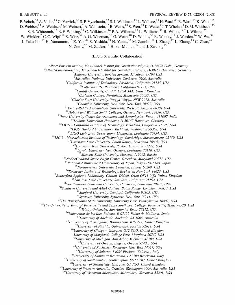
described above, is part of the C-based LSC AlgorithmsLibrary Applications (LALapps) stored in the LSCsoftCVS repository [20]. The code is run in a pipeline withoptions set to produce the results from a search and fromMonte Carlo simulations. Parallel jobs are run on computerclusters within the LSC, in the Condor environment [28],and the final post processing steps are performed usingMatlab [29]. The specific StackSlide pipeline used to findthe upper limits presented in this paper is shown in Fig. 3.The first three boxes on the left side of the pipeline can alsobe used to output candidates for follow-up searches.

A separate search was run for each successive 0.25 Hzband within 50–1000 Hz. The spacing in frequency used isgiven by Eq. (11). The spacing in _f was chosen as thatwhich changes the frequency by one SFT frequency binduring the observation time Tobs, i.e., so that _fTobs � �f.For simplicity Tobs � 2:778� 106 seconds ’ 32:15 dayswas chosen, which is greater than or equal to Tobs for eachinterferometer. Thus, the _f part of the parameter space wasover-covered by choosing

FIG. 3. Flow chart for the pipeline used to find the upper limitspresented in this paper using the StackSlide method.


022001-9

j� _fj ��fTobs�

1

TcohTobs� 2� 10�10 Hz s�1: (24)

Values of _f in the range �1� 10�8 Hz s�1; 0 Hz s�1were searched. This range corresponds to a search over51 values of _f, which is the same as PowerFlux used in itslow-frequency search (discussed in Sec. V D).

The sky grid used is similar to that used for the all-skysearch in [6], but with a spacing between sky-grid pointsappropriate for the StackSlide search. This grid is isotropicon the celestial sphere, with an angular spacing betweenpoints chosen for the 50–225 Hz band, such that themaximum change in Doppler shift from one sky-grid pointto the next would shift the frequency by half a bin. This isgiven by

�0 �0:5c�f

f�v sin�max

� 9:3� 10�3 rad�300 Hz

f

�; (25)

where v is the magnitude of the velocity v of the detector inthe SSB frame, and is the angle between v and the unitvector n giving the sky position of the source.Equations (24) and (25) are the same as Eqs. (19) and(22) in [7], which represent conservative choices thatover-cover the parameter space. Thus, the parameter spaceused here corresponds to that in Ref. [7], adjusted to the S4observation time, and with the exception that a stereo-graphic projection of the sky is not used. Rather an iso-tropic sky grid is used like the one used in [6].

One difficulty is that the computational cost of thesearch increases quadratically with frequency, due to theincreasing number of points on the sky grid. To reduce thecomputational time, the sky-grid spacing given in Eq. (25)was increased by a factor of 5 above 225 Hz. This repre-sents a savings of a factor of 25 in computational cost. Itwas shown through a series of simulations, comparing theupper limits in various frequency bands with and withoutthe factor of 5 increase in grid spacing, that this changesthe upper limits on average by less than 0.3%, with astandard deviation of 2%. Thus, this factor of 5 increasewas used to allow the searches in the 225–1000 Hz band tocomplete in a reasonable amount of time.

It is not surprising that the sky-grid spacing can beincreased, for at least three reasons. First, the value for�0 given in Eq. (25) applies to only a small annular regionon the sky, and is smaller than the average change. Second,only the net change in Doppler shift during the observationtime is important, which is less than the maximum Dopplershift due to the Earth’s orbital motion during a one monthrun. (If the Doppler shift were constant during the entireobservation time, one would not need to search sky posi-tions even if the Doppler shift varied across the sky. Asource frequency would be shifted by a constant amountduring the observation, and would be detected, albeit in afrequency bin different from that at the SSB.) Third, be-cause of correlations on the sky, one can detect a signal

with negligible loss of SNR much farther from its skylocation than the spacing above suggests.

2. Line cleaning

Coherent instrumental lines exist in the data which canmimic a continuous gravitational-wave signal forparameter-space points that correspond to little Dopplermodulation. Very narrow instrumental lines are removed(‘‘cleaned’’) from the data. In the StackSlide search, a lineis considered ‘‘narrow’’ if its full width is less than 5% ofthe 0.25 Hz band, or less than 0.0125 Hz. The line must alsohave been identified a priori as a known instrument arti-fact. Known lines with less than this width were cleaned byreplacing the contents of bins corresponding to lines withrandom values generated by using the running median tofind the mean power using 101 bins from either side of thelines. This method is also used to estimate the noise, asdescribed in Sec. VA.

It was found when characterizing the data that a comb ofnarrow 1 Hz harmonics existed in the H1 and L1 data, asshown in Fig. 4. Table II shows the lines cleaned during theStackSlide search. As the table shows, only this comb ofnarrow 1 Hz harmonics and injected lines used for calibra-tion were removed. As an example of the cleaning process,Fig. 5 shows the amplitude spectral density estimated from10 SFTs before and after line cleaning, for the band withthe 1 Hz line at 150 Hz.

The cleaning of very narrow lines has a negligible effecton the efficiency to detect signals. Very broad lines, on theother hand, cannot be handled in this way. Bands with verybroad lines were searched without any line cleaning. There

145 146 147 148 149 150 151 152 153 154 155

1

1.5

2

Frequency (Hz)

Sta

ckS

lide

Pow

er; N

o S

lidin

g

145 146 147 148 149 150 151 152 153 154 155

1

1.5

2

Frequency (Hz)

Sta

ckS

lide

Pow

er; N

o S

lidin

g

FIG. 4 (color online). The StackSlide Power for the 145–155 Hz band with no sliding. Harmonics of 1 Hz instrumentallines are clearly seen in H1 (top) and L1 (bottom). These linesare removed from the data by the StackSlide and Hough searchesusing the method described in the text, while PowerFlux searchtracks these lines and avoids them when setting upper limits.


022001-10

were also a number of highly disturbed bands, dominatedeither by the harmonics of 60 Hz power lines or by theviolin modes of the suspended optics, that were excludedfrom the StackSlide results. (Violin modes refer to resonant

excitations of the steel wires that support the interferome-ter mirrors.) These are shown in Table III. While thesebands can be covered by adjusting the parameters used tofind outliers and set upper limits, we will wait for futureruns to do this.

3. Upper limits method

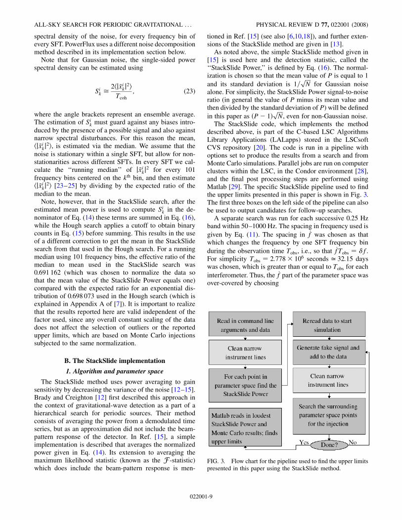
After the lines are cleaned, the powers in the SFTs arenormalized and the parameter space searched, with eachtemplate producing a value of the StackSlide Power, de-fined in Eq. (16). For this paper, only the ‘‘loudest’’StackSlide Power is kept, resulting in a value Pmax

for each 0.25 Hz band, and these are used to set upperlimits on the gravitational-wave amplitude, h0. (The loud-est coincident outliers are also identified, but none surviveas candidates after follow-up studies described inSec. VII A 1.) The upper limits are found by a series ofMonte Carlo simulations, in which signals are injected insoftware with a fixed value for h0, but with otherwiserandomly chosen parameters, and the parameter-spacepoints that surround the injection are searched. The numberof times the loudest StackSlide Power found during theMonte Carlo simulations is greater than or equal to Pmax isrecorded, and this is repeated for a series of h0 values. The95% confidence upper limit is defined to be the value of h0

that results in a detected StackSlide Power greater than orequal to Pmax 95% of the time. As shown in Fig. 3, the linecleaning described above is done after each injection isadded to the input data, which folds any loss of detectionefficiency due to line cleaning into the upper limits self-consistently.

Figure 6 shows the measured confidence versus h0 for anexample frequency band. The upper-limit finding process

TABLE III. Frequency bands excluded from the StackSlidesearch.

Excluded Bands (Hz) Description

[57, 63) Power linesn60� 1; n60� 1� n � 2 to 16 Power line harmonics[340, 350) Violin modes[685, 690) Violin mode harmonics[693, 696) Violin mode harmonics

4.2 4.3 4.4 4.5 4.6 4.7 4.8

x 10−24

0.91

0.92

0.93

0.94

0.95

0.96

0.97

0.98

0.99

h0

conf

iden

ce

measurementsbest fit linebest fit ULestimated UL

FIG. 6 (color online). Measured confidence vs h0 for an ex-ample band (140–140.25 Hz in H1). A best-fit straight line isused to find the value of h0 corresponding to 95% confidence andto estimate the uncertainties in the results (see text).

149.992 149.994 149.996 149.998 150 150.002 150.004 150.006 150.008

10−22

Frequency (Hz)

Spe

ctra

l Den

sity

(st

rain

/Hz1/

2 )

without cleaningwith cleaning

FIG. 5. The L1 amplitude spectral density in a narrow fre-quency band estimated from 10 SFTs before and after the linecleaning used by the StackSlide pipeline. In the band shown, the150 Hz bin, and one bin on either side of this bin have beenreplaced with estimates of the noise based on neighboring bins.

TABLE II. Instrumental lines cleaned during the StackSlidesearch. The frequencies cleaned are found by starting with thatgiven in the second column, and then taking steps in frequencygiven in the third column, repeating this the number of timesshown in the fourth column; the fifth and sixth columns showhow many additional Hz are cleaned to the immediate left andright of each line.

IFO fstart (Hz) fstep (Hz) Num. �fleft (Hz) �fright (Hz) Description

H1 46.7 — 1 0.0 0.0 Cal. LineH1 393.1 — 1 0.0 0.0 Cal. LineH1 973.3 — 1 0.0 0.0 Cal. LineH1 1144.3 — 1 0.0 0.0 Cal. LineH1 0.0 1.0 1500 0.0006 0.0006 1 Hz Comb

L1 54.7 — 1 0.0 0.0 Cal. LineL1 396.7 — 1 0.0 0.0 Cal. LineL1 1151.5 — 1 0.0 0.0 Cal. LineL1 0.0 1.0 1500 0.0006 0.0006 1 Hz Comb


022001-11

involves first making an initial guess of its value, thenrefining this guess using a single set of injections to findan estimate of the upper limit, and finally using this esti-mate to run several sets of injections to find the final valueof the upper limit. These steps are now described in detail.

To start the upper-limit finding process, first an initialguess, hguess

0 , is used as the gravitational-wave amplitude.The initial guess need not be near the sought-after upperlimit, just sufficiently large, as explained below. A singleset of n injections is done (specifically n � 3000 was used)with random sky positions and isotropically distributedspin axes, but all with amplitude hguess

0 . The output list ofStackSlide Powers from this set of injections is sorted inascending order and the 0:05nth (specifically for n � 3000the 150th) smallest value of the StackSlide Power is found,which we call P0:05. Note that the goal is to find the value ofh0 that makes P0:05 � Pmax, so that 95% of the outputpowers are greater than the maximum power found duringthe search. This is what we call the 95% confidence upperlimit. Of course, in general P0:05 will not equal Pmax unlessour first guess was very lucky. However, as per the dis-cussion concerning Eq. (B5), P� 1 is proportional to h2

0(i.e., removing the mean value due to noise leaves onaverage the power due to the presence of a signal). Thus,an estimate of the 95% h0 confidence upper limits is givenby the following rescaling of hguess

0 ,

hest0 �

��Pmax � 1p��P0:05 � 1p hguess

0 : (26)

Thus an estimated upper limit, hest0 , is found from a single

set of injections with amplitude hguess0 ; the only require-

ment is that hguess0 is chosen loud enough to make P0:05 > 1.

It is found that using Eq. (26) results in an estimate of theupper limit that is typically within 10% of the final value.For example, the estimated upper limit found in this way isindicated by the circled point in Fig. 6. The value of hest

0then becomes the first value for h0 in a series ofMonte Carlo simulations, each with 3000 injections, whichuse this value and 8 neighboring values, measuring theconfidence each time. The Matlab [29] polyfit and polyvalfunctions are then used to find the best-fit straight line todetermine the value of h0 corresponding to 95% confidenceand to estimate the uncertainties in the results. This is thefinal step of the pipeline shown in Fig. 3.

C. The Hough transform implementation

1. Description of algorithm

The Hough transform is a general method for patternrecognition, invented originally to analyze bubble chamberpictures from CERN [30,31]; it has found many applica-tions in the analysis of digital images [32]. This method hasalready been used to analyze data from the second sciencerun (S2) of the LIGO detectors [7] and a detailed descrip-tion can be found in [10]. Here we present only a brief

description, emphasizing the differences between the pre-vious S2 search and the S4 search described here.

The Hough search uses a weighted sum of the binarycounts as its final statistic, as given by Eqs. (15) and (19).In the standard Hough search as presented in [7,10], theweights are all set to unity. The weighted Hough transformwas originally discussed in [16]. The software for perform-ing the Hough transform has been adapted to use arbitraryweights without any significant loss in computational effi-ciency. Furthermore, the robustness of the Hough trans-form method in the presence of strong transientdisturbances is not compromised by using weights becauseeach SFT contributes at mostwi (which is of order unity) tothe final number count.

The following statements can be proven using the meth-ods of [10]. The mean number count in the absence of asignal is �n � Np, where N is the number of SFTs and p isthe probability that the normalized power, of a givenfrequency bin and SFT defined by Eq. (14), exceeds athreshold th, i.e., p is the probability that a frequencybin is selected in the absence of a signal. For unity weight-ing, the standard deviation is simply � �

��Np�1� p�

p.

However, with more general weighting, it can be shownthat � is given by

� ��jjwjj2p�1� p�

q; (27)

where jjwjj2 �PN�1i�0 w2

i . A threshold nth on the numbercount corresponding to a false-alarm rate �H is given by

nth � Np��2jjwjj2p�1� p�

qerfc�1�2�H�: (28)

Therefore nth depends on the weights of the correspondingtemplate �. In this case, the natural detection statistic is notthe ‘‘Hough number count’’ n, but the significance of anumber count, defined by

s �n� �n�

; (29)

where �n and � are the expected mean and standard devia-tion for pure noise. Values of s can be compared directlyacross different templates characterized by differingweight distributions.

The threshold th (c.f. Eq. (15)) is selected to give theminimum false-dismissal probability �H for a given false-alarm rate. In [7] it was shown that the optimal choice forth is 1.6 which corresponds to a peak selection probabilityp � e�th � 0:2. It can be shown that the optimal choice isunchanged by the weights and hence th � 1:6 is usedonce more [33].

Consider a population of sources located at a given pointin the sky, but having uniformly distributed spin axisdirections. For a template that is perfectly matched infrequency, spin-down, and sky position, and given theoptimal peak selection threshold, it can be shown [33]that the weakest signal that can cross the threshold nth


022001-12

with a false-dismissal probability �H has an amplitude

h0 � 3:38S1=2

�jjwjjw �X

�1=2

��1

Tcoh

s; (30)

where

S � erfc�1�2�H� � erfc�1�2�H�; (31)

Xi �1

Sif�Fi��

2 � �Fi��2g: (32)

As before, Fi� and Fi� are the values of the beam-patternfunctions at the midpoint of the ith SFT. To derive (30) wehave assumed that the number of SFTs N is sufficientlylarge and that the signal is weak [10].

From (30) it is clear that the scaling of the weights doesnot matter; wi ! kwi leaves h0 unchanged for any constantk. More importantly, it is also clear that the sensitivity isbest, i.e. h0 is minimum, when w �X is maximum:

wi / Xi: (33)

This result is equivalent to Eq. (18).In addition to improving sensitivity in single-

interferometer analysis, the weighted Hough method al-lows automatic optimal combination of Hough counts frommultiple interferometers of differing sensitivities.

Ideally, to obtain the maximum increase in sensitivity,we should calculate the weights for each sky locationseparately. In practice, we break up the sky into smallerpatches and calculate one weight for each sky-patch center.The gain from using the weights will be reduced if the skypatches are too large. From Eq. (32), it is clear that thedependence of the weights on the sky position is onlythrough the beam-pattern functions. Therefore, the skypatch size is determined by the typical angular scale overwhich F� and F� vary; thus for a spherical detector usingthe beam-pattern weights would not gain us any sensitivity.For the LIGO interferometers, we have investigated thisissue with Monte Carlo simulations using randomGaussian noise. Signals are injected in this noise corre-sponding to the H1 interferometer at a sky location��0; �0�, while the weights are calculated at a mismatchedsky position ��0 � �; �0 � ��. The significance valuesare compared with the significance when no weights areused. An example of such a study is shown in Fig. 7. Here,we have injected a signal at � � � � 0, cos� � 0:5, zerospin-down, �0 � � 0, and a signal-to-noise ratio corre-sponding approximately to a 6-� level without weights.The figure shows a gain of�10% at � � 0, decreasing tozero at � � 0:3 rad. We get qualitatively similar resultsfor other sky locations, independent of frequency and otherparameters. There is an additional gain due to the non-stationarity of the noise itself, which depends, however, onthe quality of the data. In practice, we have chosen to breakthe sky up into 92 rectangular patches in which the averagesky patch size is about 0.4 rad wide, corresponding to a

maximum sky-position mismatch of � � 0:2 rad inFig. 7.

2. The Hough pipeline

The Hough analysis pipeline for the search and forsetting upper limits follows roughly the same scheme asin [7]. In this section we present a short description of thepipeline, mostly emphasizing the differences from [7] andfrom the StackSlide and PowerFlux searches. As discussedin the previous subsection, the key differences from the S2analysis [7] are (i) using the beam-pattern and noiseweights, and (ii) using SFTs from multiple interferometers.

The total frequency range analyzed is 50–1000 Hz, witha resolution �f � 1=Tcoh as in (11). The resolution in _f is2:2� 10�10 Hz s�1 given in (24), and the reference timefor defining the spin-down is the start time of the observa-tion. However, unlike StackSlide and PowerFlux, theHough search is carried out over only 11 values of _f,including zero, in the range [� 2:2� 10�9 Hz s�1,0 Hz s�1]. This choice is driven by the technical designof the current implementation, which uses look-up tablesand partial Hough maps as in [7]. This implementation ofthe Hough algorithm is efficient when analyzing all resolv-able points in _f, as given in (24), but this approach isincompatible with the larger _f step sizes used in the othersearch methods, which permit those searches to search alarger _f range for comparable computational cost.

The sky resolution is similar to that used by theStackSlide method for f < 225 Hz as given by (25). Atfrequencies higher than this, the StackSlide sky resolutionis 5 times coarser, thus the Hough search is analyzing about25 more templates at a given frequency and spin-downvalue. In each of the 92 sky patches, by means of the

6.6

6.7

6.8

6.9

7

7.1

7.2

7.3

7.4

0 0.1 0.2 0.3 0.4 0.5 0.6

Sig

nific

ance

Sky Position Mismatch (radians)

With WeightsWithout Weights

FIG. 7 (color online). The improvement in the significance as afunction of the mismatch in the sky position. A signal is injectedin fake noise at � � � � 0 and the weights are calculated at� � � � �. The curve is the observed significance as a func-tion of � while the horizontal line is the observed significancewhen no weights are used. See main text for more details.


022001-13

stereographic projection, the sky patch is mapped to a two-dimensional plane with a uniform grid of that resolution�0. Sky patches slightly overlap to avoid gaps amongthem (see [7] for further details).

Figure 8 shows examples of histograms of the numbercounts in two particular sky patches for the H1 detector inthe 150–151 Hz band. In all the bands free of instrumentaldisturbances, the Hough number count distributions fol-lows the expected theoretical distribution, which can beapproximated by a Gaussian distribution. Since the numberof SFTs for H1 is 1004, the corresponding mean �n � 202:7and the standard deviation is given by Eq. (27). Thestandard deviation is computed from the weights w andvaries among different sky patches because of varyingantenna pattern functions.

The upper limits on h0 are derived from the loudestevent, registered over the entire sky and spin-down rangein each 0.25 Hz band, not from the highest number count.

As for the StackSlide method, we use a frequentist method,where upper limits refer to a hypothetical population ofisolated spinning neutron stars which are uniformly dis-tributed in the sky and have a spin-down rate _f uniformlydistributed in the range [� 2:2� 10�9 Hz s�1, 0 Hz s�1].We also assume uniform distributions for the parameterscos� 2 �1; 1, 2 0; 2�, and �0 2 0; 2�. The strat-egy for calculating the 95% upper limits is roughly thesame scheme as in [7], except for the treatment of narrowinstrumental lines.

Known spectral disturbances are removed from theSFTs in the same way as for the StackSlide search. Theknown spectral lines are, of course, also consistently re-moved after each signal injection when performing theMonte Carlo simulations to obtain the upper limits.

The narrow instrumental lines cleaned from the SFTdata are the same ones cleaned during the StackSlidesearch shown in Table II, together with ones listed in

TABLE IV. Instrumental lines cleaned during the Hough search that were not listed in Table II(see text).

IFO fstart (Hz) fstep (Hz) n �fleft (Hz) �fright (Hz) Description

H1 392.365 — 1 0.01 0.01 Cal. SideBandH1 393.835 — 1 0.01 0.01 Cal. SideBand

H2 54.1 — 1 0.0 0.0 Cal. LineH2 407.3 — 1 0.0 0.0 Cal. LineH2 1159.7 — 1 0.0 0.0 Cal. LineH2 110.934 36.9787 4 0.02 0.02 37 Hz Oscillator

L1 154.6328 8.1386 110 0.01 0.01 8.14 Hz CombL1 0.0 36.8725 50 0.02 0.02 37 Hz Oscillatora

aThese lines were removed only in the multi-interferometer search.

120 140 160 180 200 220 240 260 280 300 320

0

0.005

0.01

0.015

0.02

0.025

0.03

H1 number count

H1 150−151 Hz, north pole patch

Hou

gh n

orm

pdf

measurednormpdf

100 120 140 160 180 200 220 240 260 280 3000

0.005

0.01

0.015

0.02

0.025

H1 number count

H1 150−151 Hz, equator patch

Hou

gh n

orm

pdf

measurednormpdf

FIG. 8 (color online). Two example histograms of the normalized Hough number count compared to a Gaussian distribution for theH1 detector in the frequency band 150–151 Hz. The left figure corresponds to a patch located at the north pole for the case in which theweights are used. The number of templates analyzed in this 1 Hz band is of 11� 106, the number of SFTs 1004, the correspondingmean �n � 202:7, and � � 12:94 is obtained from the weights. The right figure corresponds to a patch at the equator using the samedata. In this case the number of templates analyzed in this 1 Hz band is of 10:5� 106, and its corresponding � � 14:96.


022001-14

Table IV. The additional lines listed in Table IVare cleanedto prevent large artifacts in one instrument from increasingthe false-alarm rate of the Hough multi-interferometersearch. Note that the L1 36.8725 Hz comb was eliminatedmidway through the S4 run by replacing a synthesizedradio frequency oscillator for phase modulation with acrystal oscillator, and these lines were not removed in theHough L1 single-interferometer analysis.

No frequency bands have been excluded from the Houghsearch, although the upper limits reported on the bandsshown in Table III, that are dominated by 60 Hz power lineharmonics or violin modes of the suspended optics, did notalways give satisfactory convergence to an upper limit. In afew of these very noisy bands, upper limits were set byextrapolation, instead of interpolation, of the Monte Carlosimulations. Therefore the results reported on those bandshave larger error bars. No parameter tuning was performedon these disturbed bands to improve the upper limits.

D. The PowerFlux implementation

The PowerFlux method is a variant on the StackSlidemethod in which the contributions from each SFT areweighted by the inverse square of the average spectralpower density in each band and weighted according tothe antenna pattern sensitivity of the interferometer foreach point searched on the sky. This weighting scheme

has two advantages: (1) variance on the signal strengthestimator is minimized, improving signal-to-noise ratio;and (2) the estimator is itself a direct measure of sourcestrain power, allowing direct parameter estimation anddramatically reducing dependence on Monte Carlo simu-lations. Details of software usage and algorithms can befound in a technical document [17]. Figure 9 shows a flowchart of the algorithm, discussed in detail below.

1. Noise decomposition

Noise estimation is carried out through a time/frequencynoise decomposition procedure in which the dominantvariations are factorized within each nominal 0.25 Hzband as a product of a spectral variation and a time varia-tion across the data run. Specifically, for each 0.25 Hzband, a matrix of logarithms of power measurementsacross the 0.56 mHz SFT bins and across the SFT’s ofthe run is created. Two vectors, denoted TMedians andFMedians, are initially set to zero and then iterativelyupdated according to the following algorithm:

(1) For each SFT (row in matrix), the median value(logarithm of power) is computed and then addedto the corresponding element of TMedians whilesubtracted from each matrix element in that row.

(2) For each frequency bin (column in matrix), themedian value is computed and then added to thecorresponding FMedians element, while subtractedfrom each matrix element in that column.

(3) The procedure repeats from step 1 until all medianscomputed in steps 1 and 2 are zero (or negligible).

The above algorithm typically converges quickly. The sizeof the frequency band treated increases with central fre-quency, as neighboring bins are included to allow formaximum and minimum Doppler shifts to be searched inthe next step.

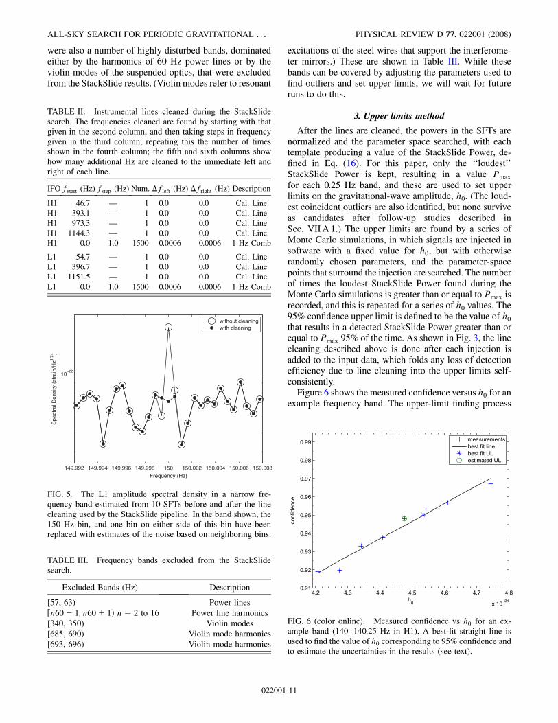
For stationary, Gaussian noise and for noise that followsthe above assumptions of underlying factorized frequencyand time dependence, the expected distribution of residualmatrix values can be found from simulation. Figure 10shows a sample expected residual power distribution fol-lowing noise decomposition for simulated stationary,Gaussian data, along with a sample residual power distri-bution from the S4 data (0.25 Hz band of H1 near 575 Hz,in this case) following noise decomposition. The agree-ment in shape between these two distributions is very goodand is typical of the S4 data, despite sometimes largevariations in the corresponding TMedians and FMediansvectors, and despite, in this case, the presence of a moder-ately strong simulated pulsar signal (Pulsar2 in Table V).

The residuals are examined for outliers. If the largestresidual value is found to lie above a threshold of 1.5, thatcorresponding 0.25 Hz band is flagged as containing a‘‘wandering line’’ because a strong but drifting instrumen-tal line can lead to such outliers. The value 1.5 is deter-

FIG. 9. Flow chart for the pipeline used to find the upper limitspresented in this paper using the PowerFlux method.


022001-15

mined empirically from Gaussian simulations. An ex-tremely strong pulsar could also be flagged in this way,and indeed the strongest injected pulsars are labeled aswandering lines. Hence in the search, the wandering linesare followed up, but no upper limits are quoted here for theaffected bands.

2. Line flagging

Sharp instrumental lines can prevent accurate noiseestimation for pulsars that have detected frequencies inthe same 0.56 mHz bin as the line. In addition, strong linestend to degrade achievable sensitivity by adding excessapparent power in an affected search. In early LIGO sci-

ence runs, including the S4 run, there have been sharpinstrumental lines at multiples of 1 Hz or 0.25 Hz, arisingfrom artifacts in the data acquisition electronics.

To mitigate the most severe of these effects, thePowerFlux algorithm performs a simple line detectionand flagging algorithm. For each 0.25 Hz band, the de-tected summed powers are ranked and an estimatedGaussian sigma computed from the difference in the 50%and 94% quantiles. Any bins with power greater than 5:0�are marked for ignoring in subsequent processing.Specifically, when carrying out a search for a pulsar of anominal true frequency, its contribution to the signal esti-mator is ignored when the detected frequency would lie inthe same 0.56 mHz bin as a detected line. As discussedbelow, for certain frequencies, spin-downs, and points inthe sky, the fraction of time a putative pulsar has a detectedfrequency in a bin containing an instrumental line can bequite large, requiring care. The deliberate ignoring ofcontributing bins affected by sharp instrumental linesdoes not lead to a bias in resulting limits, but it doesdegrade sensitivity, from loss of data. In any 0.25 Hzband, no more than five bins may be flagged as lines.Any band with more than five line candidates is examinedmanually.

3. Signal estimator

Once the noise decomposition is complete, with esti-mates of the spectral noise density for each SFT, thePowerFlux algorithm computes a weighted sum of thestrain powers, where the weighting takes into account theunderlying time and spectral variation contained inTMedians and FMedians and the antenna pattern sensitiv-ity for an assumed sky location and incident wave polar-ization. Specifically, for an assumed polarization angle and sky location, the following quantity is defined for eachbin k of each SFT i:

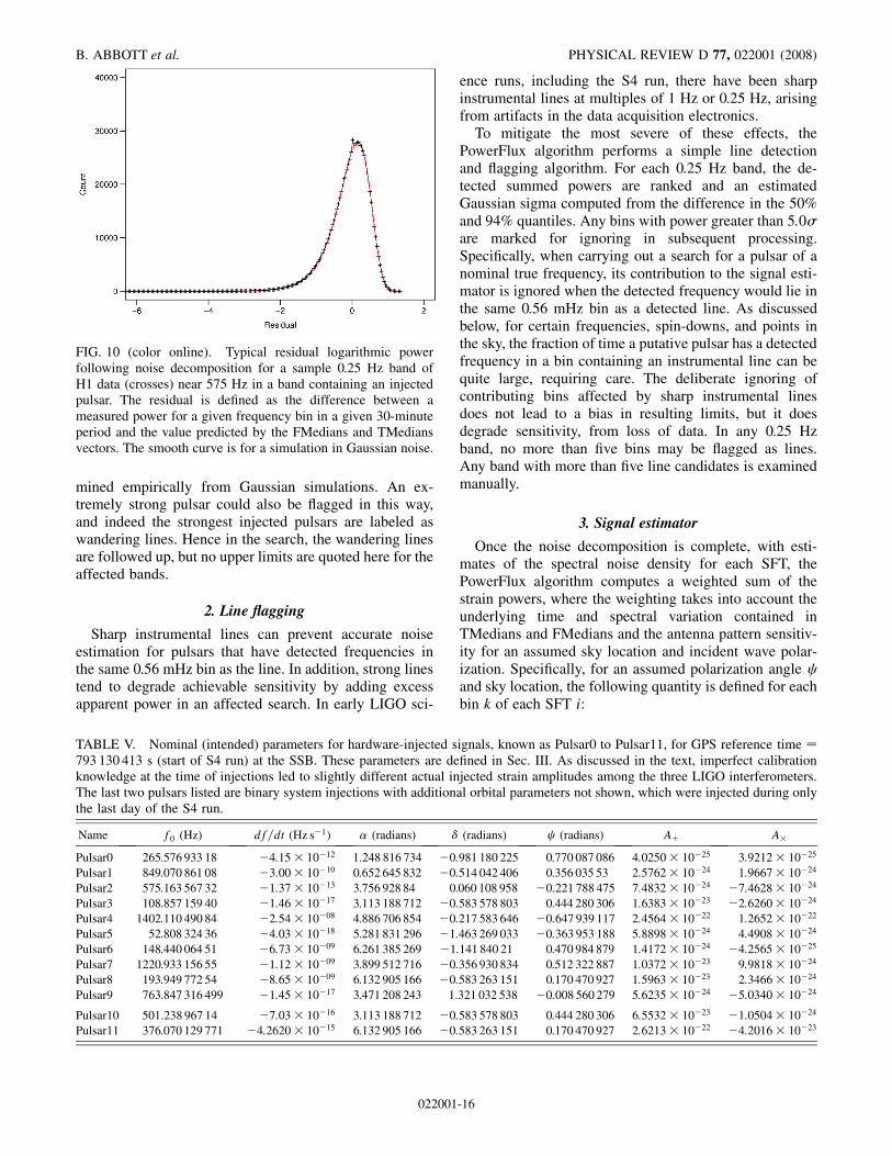
TABLE V. Nominal (intended) parameters for hardware-injected signals, known as Pulsar0 to Pulsar11, for GPS reference time �793 130 413 s (start of S4 run) at the SSB. These parameters are defined in Sec. III. As discussed in the text, imperfect calibrationknowledge at the time of injections led to slightly different actual injected strain amplitudes among the three LIGO interferometers.The last two pulsars listed are binary system injections with additional orbital parameters not shown, which were injected during onlythe last day of the S4 run.

Name f0 (Hz) df=dt (Hz s�1) � (radians) � (radians) (radians) A� A�

Pulsar0 265.576 933 18 �4:15� 10�12 1.248 816 734 �0:981 180 225 0.770 087 086 4:0250� 10�25 3:9212� 10�25

Pulsar1 849.070 861 08 �3:00� 10�10 0.652 645 832 �0:514 042 406 0.356 035 53 2:5762� 10�24 1:9667� 10�24

Pulsar2 575.163 567 32 �1:37� 10�13 3.756 928 84 0.060 108 958 �0:221 788 475 7:4832� 10�24 �7:4628� 10�24

Pulsar3 108.857 159 40 �1:46� 10�17 3.113 188 712 �0:583 578 803 0.444 280 306 1:6383� 10�23 �2:6260� 10�24

Pulsar4 1402.110 490 84 �2:54� 10�08 4.886 706 854 �0:217 583 646 �0:647 939 117 2:4564� 10�22 1:2652� 10�22

Pulsar5 52.808 324 36 �4:03� 10�18 5.281 831 296 �1:463 269 033 �0:363 953 188 5:8898� 10�24 4:4908� 10�24

Pulsar6 148.440 064 51 �6:73� 10�09 6.261 385 269 �1:141 840 21 0.470 984 879 1:4172� 10�24 �4:2565� 10�25

Pulsar7 1220.933 156 55 �1:12� 10�09 3.899 512 716 �0:356 930 834 0.512 322 887 1:0372� 10�23 9:9818� 10�24

Pulsar8 193.949 772 54 �8:65� 10�09 6.132 905 166 �0:583 263 151 0.170 470 927 1:5963� 10�23 2:3466� 10�24

Pulsar9 763.847 316 499 �1:45� 10�17 3.471 208 243 1.321 032 538 �0:008 560 279 5:6235� 10�24 �5:0340� 10�24

Pulsar10 501.238 967 14 �7:03� 10�16 3.113 188 712 �0:583 578 803 0.444 280 306 6:5532� 10�23 �1:0504� 10�24

Pulsar11 376.070 129 771 �4:2620� 10�15 6.132 905 166 �0:583 263 151 0.170 470 927 2:6213� 10�22 �4:2016� 10�23

FIG. 10 (color online). Typical residual logarithmic powerfollowing noise decomposition for a sample 0.25 Hz band ofH1 data (crosses) near 575 Hz in a band containing an injectedpulsar. The residual is defined as the difference between ameasured power for a given frequency bin in a given 30-minuteperiod and the value predicted by the FMedians and TMediansvectors. The smooth curve is for a simulation in Gaussian noise.


022001-16

Qi �Pi�Fi �

2 ; (34)

where Fi is the -dependent antenna pattern for the skylocation, defined in Eq. (22). (See also Appendix A.)

As in Sec. IV B, to simplify the notation we define Qi �

Pi=�Fi �

2 as the value of Qi for SFT i and a given template�.

For each individual SFT bin power measurement Pi, oneexpects an underlying exponential distribution, with astandard deviation equal to the mean, a statement thatholds too for Qi. To minimize the variance of a signalestimator based on a sum of these powers, each contribu-tion is weighted by the inverse of the expected variance ofthe contribution. Specifically, we compute the followingsignal estimator:

R �2

Tcoh

�Xi

1

� �Qi�2

��1X

i

Qi

� �Qi�2; (35)

�2

Tcoh

�Xi

�Fi �22

� �Pi�2

��1X

i

�Fi �2Pi

� �Pi�2 ; (36)

where �Pi and �Qi are the expected uncorrected and antenna-corrected powers of SFT i averaged over frequency. Sincethe antenna factor is constant in this average, �Qi ��Pi=�Fi �

2. Furthermore, �Pi is an estimate of the powerspectral density of the noise. The replacement �Pi � Sigives Eq. (20).

Note that for a SFT iwith low antenna pattern sensitivityjFi j, the signal estimator receives a small contribution.Similarly, SFT’s i for which ambient noise is high receivesmall contributions. Because computational time in thesearch grows linearly with the number of SFT’s and be-cause of large time variations in noise, it proves efficient toignore SFT’s with sky-dependent and polarization-dependent effective noise higher than a cutoff value. Thecutoff procedure saves significant computing time, withnegligible effect on search performance.

Specifically, the cutoff is computed as follows. Let �j bethe ordered estimated standard deviations in noise, taken tobe the ordered means of �Qi �

1kmax

�k�Qik, where kmax is the

number of frequency bins used in the search template.Define jopt to be the index jmax for which the quantity

1jmax

��jmaxj�1�

2j

qis minimized. Only SFT’s for which �j <

2�joptare used for signal estimation. In words, jopt defines

the last SFT that improves rather than degrades signalestimator variance in an unweighted mean. For theweighted mean used here, the effective noise contributionsare allowed to be as high as twice the value found for jopt.The choice of 2�jopt

is determined empirically.The PowerFlux search sets strict, frequentist, all-sky

95% confidence-level upper limits on the flux of gravita-

tional radiation bathing the Earth. To be conservative in thestrict limits, numerical corrections to the signal estimatorare applied: (1) a factor of 1= cos��=8� � 1:082 for maxi-mum linear-polarization mismatch, based on twice themaximum half-angle of mismatch (see Appendix A);(2) a factor of 1.22 for bin-centered signal power lossdue to Hann windowing (applied during SFT generation);and (3) a factor of 1.19 for drift of detected signal fre-quency across the width of the 0.56 mHz bins used in theSFT’s. Note that the use of rectangular windowing wouldeliminate the need for correction (2) above, but wouldrequire a larger correction of 1.57 for (3).

Antenna pattern and noise weighting in the PowerFluxmethod allows weaker sources to be detected in certainregions of the sky, where run-averaged antenna patternsdiscriminate in declination and diurnal noise variationsdiscriminate in right ascension. Figure 11 illustrates theresulting variation in effective noise across the sky for a0.25 Hz H1 band near 575 Hz for the circular-polarizationprojection. By separately examining SNR, one may hope todetect a signal in a sensitive region of the sky with a strainsignificantly lower than suggested by the strict worst-caseall-sky frequentist limits presented here, as discussed be-low in Sec. VI D. Searches are carried out for four linearpolarizations, ranging over polarization angle from � 0to � 3

8� in steps of �=8 and for (unique) circularpolarization.

A useful computational savings comes from definingtwo different sky resolutions. A ‘‘coarse’’ sky gridding isused for setting the cutoff value defined above, while finegrid points are used for both frequency and amplitudedemodulation. A typical ratio of number of coarse gridpoints to number of fine grid points used for Dopplercorrections is 25.

4. Sky banding

Stationary and near-stationary instrumental spectrallines can be mistaken for a periodic source of gravitationalradiation if the nominal source parameters are consistentwith small variation in detected frequency during the time

FIG. 11 (color). Sky map of run-summed PowerFlux weightsfor a 0.25 Hz band near 575 Hz for one choice of linearpolarization in the S4 H1 data. The normalization correspondsroughly to the effective number of median-noise SFT’s contrib-uting to the sum.


022001-17

of observation. The variation in the frequency at the detec-tor can be found by taking the time derivative of Eq. (9),which gives

dfdt�

�1�

v�t� � nc

�_f� f�t�

a�t� � nc

: (37)

The detector’s acceleration a in this equation is dominatedby the Earth’s orbital acceleration aEarth, since the diurnalpart of the detector’s acceleration is small and approxi-mately averages to zero during the observation. Thus, itshould be emphasized that a single instrumental line canmimic sources with a range of slightly different frequenciesand assumed different positions in the sky that lie in anannular band. For a source _f assumed to be zero, the centerof the band is defined by a circle 90 degrees away from thedirection of the average acceleration of the Earth during therun where �aEarth � n � 0, i.e., toward the average directionof the Sun during the run. For source spin-downs differentfrom zero, there can be a large cancellation between as-sumed spin-down (or spin-up) and the Earth’s averageacceleration, leading to a shift of the annular region ofapparent Doppler stationarity toward (away from) the Sun.

A figure of merit found to be useful for discriminatingregions of ‘‘good’’ sky from ‘‘bad’’ sky (apparent detectedfrequency is highly stationary) is the ‘‘S parameter’’:

S � _f� �� vEarth=c� � n�f0; (38)

where � is the Earth’s angular velocity vector about thesolar system barycenter. The term �� vEarth is a measureof the Earth’s average acceleration during the run, wherevEarth is taken to be the noise-weighted velocity of the H1detector during the run. Regions of sky with small jSj for agiven f and _f have stationary detected frequency. Asdiscussed below in Sec. VI D, such regions are not onlyprone to high false-alarm rates, but the line flagging pro-cedure described in Sec. V D 2 leads to systematicallyunderestimated signal strength and invalid upper limits.Hence limits are presented here for only sources with jSjgreater than a threshold value denoted Slarge. The minimumacceptable value chosen for Slarge is found from softwaresignal injections to be 1:1� 10�9 Hz s�1 for the 1-monthS4 run and can be understood to be

Slarge �Noccupied bins

Tobs � Tcoh; (39)

where Noccupied bins � 5 is the minimum total number of0.56 mHz detection bins occupied by the source duringthe data run for reliable detection. In practice, we usestill larger values for the H1 interferometer (Slarge �

1:85� 10�9 Hz s�1) and L1 interferometer (Slarge �

3:08� 10�9 Hz s�1) during the S4 run for the limits pre-sented here because of a pervasive and strong comb ofprecise 1 Hz lines in both interferometers. These lines,

caused by a global positioning system (GPS)-second syn-chronized electronic disturbance and worse in L1 than inH1, lead to high false-alarm rates from that data for lowervalues of Slarge. For the frequency and spin-down ranges

a)

Right Ascension

Dec

linat

ion

•

b)

Right Ascension

Dec

linat

ion

•

c)

Right Ascension

Dec

linat

ion

•

FIG. 12. S4 sky band regions (good—light gray, bad forL1—medium or dark gray, bad for H1 and L1—dark gray)for a source frequency f � 100 Hz and three different assumedspin-down choices: (a) zero; (b) �3� 10�9 Hz s�1; and(c) �1� 10�8 Hz s�1. The black circle indicates the averageposition of the Sun during the data run.

a)

Right Ascension

Dec

linat

ion

•

b)

Right Ascension

Dec

linat

ion

•

c)

Right Ascension

Dec

linat

ion

•

FIG. 13. S4 sky band regions (good—light gray, bad forL1—medium or dark gray, bad for H1 and L1—dark gray)for a source frequency f � 300 Hz and three different assumedspin-down choices: (a) zero; (b) �3� 10�9 Hz s�1; and(c) �1� 10�8 Hz s�1. The black circle indicates the averageposition of the Sun during the data run.


022001-18

searched in this analysis, the average fractions of sky lostto the sky band veto are 15% for H1 and 26% for L1.

Figures 12–14 illustrate the variation in the fraction ofsky marked as bad as assumed source frequency and spin-down are varied. Generally, at low frequencies, large skyregions are affected, but only for low spin-down magni-tude, while at high frequencies, small sky regions areaffected, but the effects are appreciable to larger spin-down magnitude. It should be noted that the annular re-gions of the sky affected depend upon the start time andduration of a data run. The longer the data run, the smallerthe region of sky for which Doppler stationarity is small.Future LIGO data runs of longer duration should have onlysmall regions near the ecliptic poles for which stationaryinstrumental lines prove troublesome.

5. Grid-point upper limit determination

An intermediate step in the PowerFlux analysis is thesetting of upper limits on signal strength for each sky pointfor each 0.56 mHz bin. The limits presented here for eachinterferometer are the highest of these intermediate limitsfor each 0.25 Hz band over the entire good sky. Theintermediate limits are set under the assumption ofGaussian residuals in noise. In brief, for each 0.56 mHzbin and sky point, a Feldman-Cousins [34] 95% confidencelevel is set for an assumed normal distribution with astandard deviation determined robustly from quantiles ofthe entire 0.25 Hz band. The Feldman-Cousins approachprovides the virtues of a well-behaved upper limit even

when background noise fluctuates well below its expecta-tion value and of smooth transition between 1-sided and 2-sided limits, but in practice the highest upper limit for any0.25 Hz band is invariably the highest measured power plus1.96 times the estimated standard deviation on the back-ground power for that bin, corresponding to a conventionala priori 1-sided 97.5% upper CL. A Kolmogorov-Smirnov(KS) statistic is computed to check the actual poweragainst a Gaussian distribution for each 0.25 Hz band.Those bands that fail the KS test value of 0.07 (> 5�deviation for the S4 data sample) are flagged as ‘‘Non-Gaussian,’’ and no upper limits on pulsars are quoted herefor those bands, although a full search is carried out. Bandssubject to violin modes and harmonics of the 60 Hz powermains tend to fail the KS test because of sharp spectralslope (and sometimes because nonstationarity of sharpfeatures leads to poor noise factorization).

Figure 15 provides an example of derived upper limitsfrom one narrow band. The figure shows the distribution ofPowerFlux strain upper limits on linear-polarization am-plitude hLin

0 for a sample 0.25 Hz band of S4 H1 data near149 Hz. The highest upper limit found is 3:35� 10�24

(corresponding to a worst-case pulsar upper limit on h0 of6:70� 10�24). The bimodal distribution arises from differ-ent regions of the sky with intrinsically different antennapattern sensitivities. The peak at 2:8� 10�24 correspondsto points near the celestial equator where the run-averagedantenna pattern sensitivity is worst.

VI. HARDWARE INJECTIONS AND VALIDATION

All three methods discussed in this paper have under-gone extensive internal testing and review. Besides indi-vidual unit tests of the software, hardware injectionsprovided an end-to-end validation of the entire pipelines.

FIG. 15. Histogram of Feldman-Cousins 95% confidence-levelupper limits in a 0.25 Hz band near 149 Hz in S4 H1 data. Eachentry corresponds to the highest upper limit in the band for asingle sky location.

a)

Right Ascension

Dec

linat

ion

•

b)

Right Ascension

Dec

linat

ion

•

c)

Right Ascension

Dec

linat

ion

•

FIG. 14. S4 sky-band regions (good—light gray, bad forL1—medium or dark gray, bad for H1 and L1—dark gray)for a source frequency f � 1000 Hz and three different assumedspin-down choices: (a) zero; (b) �3� 10�9 Hz s�1; and(c) �1� 10�8 Hz s�1. The black circle indicates the averageposition of the Sun during the data run.


022001-19

The next subsections discuss the hardware injections, thevalidations of the three methods, and their pipelines. Thedetection of the hardware injections also shows in dramaticfashion that we can detect the extremely tiny signals thatthe detectors were designed to find.

A. Hardware injections

During a 15-day period in the S4 run, ten artificialisolated-pulsar signals were injected into all three LIGOinterferometers at a variety of frequencies and time deriva-tives of the frequency, sky locations, and strengths. Twoadditional artificial binary pulsar signals were injected forapproximately one day. These hardware injections wereimplemented by modulating the interferometer mirror po-sitions via signals sent to voice actuation coils surroundingmagnets glued to the mirror edges. The injections providedan end-to-end validation of the search pipelines. Table Vsummarizes the nominal parameters used in the isolated-pulsar injections; the parameters are defined in Sec. III.

Imperfect calibration knowledge at the time of theseinjections led to slightly different actual strain amplitudeinjections among the three LIGO interferometers. For theH1 and L1 comparisons between expected and detectedsignal strengths for these injections described in Sec. VI B,corrections must be applied for the differences from nomi-nal amplitudes. The corrections are the ratios of the actua-tion function derived from final calibration to the actuationfunction assumed in the preliminary calibration used dur-ing the injections. For H1 this ratio was independent of theinjection frequency and equal to 1.12. For L1, this ratiovaried slightly with frequency, with a ratio of 1.11 for allinjected pulsars except Pulsar1 (1.15) and Pulsar9 (1.18).

B. StackSlide validation

Besides individual unit tests and a review of each com-ponent of the StackSlide code, we have shown that simu-lated signals are detected with the expected StackSlide

Power, including the hardware injections listed inTable V. Table VI shows the observed and injected SNR,and the square root of the observed and injected StackSlidePower,

��Pp

. The percent difference of the latter is given,since this compares amplitudes, which are easier to com-pare with calibration errors. The observed values wereobtained by running the StackSlide code using a templatethat exactly matches the injection parameters, while theinjected values were calculated using the parameters inTable V and the equations in Appendix B. The SNR’s ofPulsar0, Pulsar1, Pulsar5, and Pulsar6 were too small to bedetected, and Pulsar4 and Pulsar7 were out of the fre-quency band of the all-sky search. Pulsar2, Pulsar3, andPulsar8 were detected as outliers with SNR> 7 (as dis-cussed in Sec. VII) while Pulsar9 was not loud enough topass this requirement. In all cases the observed StackSlidePower agrees well with that predicted, giving an end-to-end validation of the StackSlide code.

TABLE VI. Results of StackSlide analyses of the ten hardware-injected continuous gravitational-wave signals from isolated neutronstars.

H1 L1Observed Injected Observed Injected Percent Observed Injected Observed Injected Percent

Pulsar SNR SNR��Pp ��

Pp

Difference SNR SNR��Pp ��

Pp

Difference

Pulsar0 0.27 0.23 1.006 1.005 0.1% 0.15 0.13 1.003 1.003 0.1%Pulsar1 1.62 0.80 1.035 1.017 1.7% 0.27 0.69 1.006 1.016 �1:0%Pulsar2 8.92 8.67 1.179 1.175 0.4% 8.20 9.34 1.180 1.203 �1:9%Pulsar3 199.78 174.72 3.124 2.943 6.2% 89.89 104.76 2.304 2.454 �6:1%Pulsar4 2081.64 1872.24 9.607 9.116 5.4% 1279.12 1425.14 7.895 8.326 �5:2%Pulsar5 0.05 1.30 1.001 1.028 �2:6% 1.02 0.44 1.024 1.010 1.4%Pulsar6 0.17 2.94 1.004 1.063 �5:5% 2.90 1.36 1.067 1.032 3.4%Pulsar7 6.25 5.50 1.129 1.114 1.3% 6.07 5.11 1.136 1.116 1.8%Pulsar8 98.12 96.21 2.303 2.285 0.8% 92.77 103.45 2.334 2.441 �4:4%Pulsar9 6.68 6.59 1.137 1.135 0.2% 2.61 3.69 1.061 1.085 �2:2%

FIG. 16 (color). Detection of hardware-injected Pulsar 2 by theStackSlide code in the H1 (top) and L1 (bottom) data.


022001-20

As an example of an all-sky search for a band with aninjection, Fig. 16 shows the detection of Pulsar2 for asearch of the H1 (top) and L1 (bottom) data, and onlyduring the times the hardware injections were running.Later, when the entire S4 data set was analyzed Pulsar2was still detected but with lower SNR, since this dataincludes times when the hardware injections were absent.Also note that, as explained in Sec. V D, because of strongcorrelations on the sky, a pulsar signal will be detected atmany points that lie in an annular region in the sky thatsurrounds the point corresponding to the average orbitalacceleration vector of the Earth, or its antipode. In fact,because of the large number of templates searched, randomnoise usually causes the maximum detected SNR to occurin a template other than the one which is closest to havingthe exact parameters of the signal. For example, for theexact template and times matching the Pulsar2 hardwareinjection, it was detected with SNR’s of 8.92 and 8.20 in H1and L1, respectively, as given in Table VI, while the largestSNR’s shown in Fig. 16 are 13.84 and 13.29. During thesearch of the full data set (including times when Pulsar2was off) it was detected with SNR 11.09 and 10.71 in H1and L1, respectively.

C. Hough validation

Using the Hough search code, four hardware-injectedsignals have been clearly detected by analyzing the data

from the interval when the injections took place. Thesecorrespond to Pulsar2, Pulsar3, Pulsar8, and Pulsar9. Foreach of these injected signals, a small-area search(0:4 rad� 0:4 rad) was performed, using a step size onthe spin-down parameter of �4:2� 10�10 Hz s�1. Giventhe large spin-down value of Pulsar8 (� 8:65�10�9 Hz s�1), we have used 23 values of the spin-downspanning the range [� 9:24� 10�9 Hz s�1, 0 Hz s�1] tosearch for this pulsar. Because of its large amplitude,Pulsar8 can be detected even with a large mismatch inthe spin-down value, although at the cost of lower SNR.

Figure 17 shows the significance maximized over differ-ent sky locations and spin-down values for the differentfrequencies. These four hardware-injected pulsars havebeen clearly detected, with the exception of Pulsar9 inthe L1 data. Pulsar9 is marginally visible using the H1data alone, with a maximum significance of 6.13, but whenwe combine the data from the three interferometers, thesignificance increases up to 8.32. Details are given inTable VII, including the frequency range of the detectedsignal, the frequency at which the maximum significance isobtained and its significance value.

Figure 18 shows the Hough significance maps for themulti-interferometer case. The maps displayed correspondeither to the frequency and spin-down values nearest to theinjected ones, or to those in which the maximum signifi-cance was observed. The location of the injected pulsarscorrespond to the center of each map. Note that the true

575.14 575.16 575.18 575.20

5

10

15

20

Frequency (Hz)

Sig

nific

ance

Pulsar 2

MultiH1L1

108.82 108.84 108.86 108.880

10

20

30

40

Frequency (Hz)

Sig

nific

ance

Pulsar 3

193.9 193.92 193.94 193.96 193.98 1940

10

20

30

40

Frequency (Hz)

Sig

nific

ance

Pulsar 8

763.82 763.84 763.86 763.880

2

4

6

8

10

Frequency (Hz)

Sig

nific

ance

Pulsar 9

FIG. 17 (color online). Maximum significance as a function of frequency corresponding to the multi-interferometer search (using thedata from the three detectors) and the H1 and L1 alone.


022001-21

spin-down value of Pulsar8, �8:65� 10�9 Hz s�1, liesbetween the parameter values �8:82� 10�9 Hz s�1 and�8:40� 10�9 Hz s�1 of the nearest templates used.

D. PowerFlux validation

Several cross checks have been performed to validate thePowerFlux search algorithm. These validations range fromsimple and rapid Fourier-domain ‘‘power injections’’ tomore precise time-domain software simulations, to hard-ware signal injections carried out during data taking.

Signal strain power injections have been carried out aspart of PowerFlux algorithm development and for parame-ter tuning. These software injections involve superimpos-ing calculated powers for assumed signals upon the LIGOpower measurements and carrying out searches. For com-putational speed, when testing signal detection efficiency,only a small region of the sky around the known sourcedirection is searched. A critical issue is whether the strictfrequentist limits set by the algorithm are sufficiently con-servative to avoid under-coverage of the intended frequent-

FIG. 18 (color online). Maps of the Hough significance corresponding to the multi-interferometer case for Pulsar2, Pulsar3, Pulsar8,and Pulsar9. The location of the injected pulsars are the centers of the maps. For Pulsar2, Pulsar3, and Pulsar9, the maps correspond tothe frequency and spin-down values closest to the real injected ones. For Pulsar8, we show the map containing the maximumsignificance value. The discrepancy in sky location is due to the mismatch in frequency and spin-down values between those used inthe injections and those corresponding to the Hough map.

TABLE VII. Results of the Hough search for the hardware-injected signals for the multi-interferometer, H1 and L1 data.

Pulsar Detector f0 range (Hz) f0�max� (Hz) Significance

Pulsar2 Multi-IFO 575.15–575.18 575.1689 15.1195H1 575.15–575.18 575.1667 11.1730L1 575.15–575.18 575.1650 9.7635



Pulsar9 Multi-IFO 763.83–763.87 763.8511 8.3159H1 763.83–763.87 763.8556 6.1268L1 — — 5.4559


022001-22

ist confidence band. We present here a set of figures thatconfirm over-coverage applies. Figure 19 shows the differ-ence (‘‘excess’’) between the Feldman-Cousins 95%confidence-level upper limit (conventional 97.5% upperlimit) on strain and the injected strain for a sample ofelliptic-polarization time-domain injections in the H1 in-terferometer for the 140.50–140.75 Hz band. Injectionamplitudes were distributed logarithmically, while fre-quencies, spin-downs, sky locations, and orientationswere distributed uniformly. One sees that there is indeedno under-coverage (every excess strain value is above zero)over the range of injection amplitudes. Figure 20 shows thesame excess plotted vs the injected spin-down value, wherethe search assumes a spin-down value of zero, and where

the sample includes injections with actual spin-down val-ues more than a step size away from the assumed value forthe search template. As one can see, in this frequencyrange, a spin-down step size of 1:0� 10�9 Hz s�1 is safe(true spin-down no more than 5:0� 10�10 Hz s�1 awayfrom the assumed search value). Figure 21 shows theexcess plotted vs the S parameter that discriminates be-tween sky regions of low and high Doppler stationarity. Asshown, a value of Slarge � 1� 10�9 Hz s�1 is safe for theseinjections. For this search we have chosen 51 spin-downsteps of 2� 10�10 Hz s�1 for 50–225 Hz and 11 steps of1� 10�9 Hz s�1 for 200–1000 Hz.

More computationally intensive full time-domain signalinjections were also carried out and the results found to beconsistent with those from power injections, within statis-tical errors.

In addition, the PowerFlux method was validated withthe hardware signal injections summarized in Table V. ThePowerFlux algorithm was run on all 10 isolated pulsars,including two outside the 50–1000 Hz search region, andresults found to agree well with expectation for thestrengths of the signals and the noise levels in their bands.Table VIII shows the results of the analysis for the sixpulsars for which a detection with SNR> 7 is obtained byPowerFlux for one or both of the 4 km interferometers.Figure 22 shows a sky map of PowerFlux � 0 polariza-tion SNR for the 0.25 Hz band containing pulsar 2(575.16 Hz).

VII. RESULTS

All three methods described in Secs. IVand V have beenapplied in an all-sky search over a frequency range 50–1000 Hz. As described below, no evidence for agravitational-wave signal is observed in any of thesearches, and upper limits on sources are determined. For

FIG. 20. Excess (upper limit minus injected) strain plotted vsinjected signal spin-down for sample PowerFlux H1 ellipticpolarization near 140 Hz injections.

FIG. 21. Excess (upper limit minus injected) strain plotted vs Sparameter defined in text, where values greater than 8� 10�24

have been ‘‘capped’’ at that ceiling value.

FIG. 19. Excess (upper limit minus injected) strain plotted vsinjected signal strain for sample PowerFlux H1 elliptic-polarization near 140 Hz injections.


022001-23

the StackSlide and Hough methods, 95% confidence-levelfrequentist upper limits are placed on putative rotatingneutron stars, assuming a uniform-sky and isotropic-orientation parent sample. Depending on the source loca-tion and inclination, these limits may over-cover or under-cover the true 95% confidence-level band. For thePowerFlux method, strict frequentist upper limits areplaced on linearly and circularly polarized periodicgravitational-wave sources, assuming worst-case sky loca-tion, avoiding under-coverage. The limits on linear polar-ization are also reinterpreted as limits on rotating neutronstars, assuming worst-case sky location and worst-case starinclination. The following subsections describe these re-sults in detail.

A. StackSlide results

1. Loudest powers and coincidence outliers

The StackSlide method was applied to the S4 H1 and L1data set, as given in Sec. V B. As described in that section,only the loudest StackSlide Power was returned from a

search of the entire sky, the range of the frequency’s timederivative, �1� 10�8; 0 Hz s�1, and for each 0.25 Hzband within 50–1000 Hz. The results are shown in Fig. 23.

Many of the StackSlide results have power greater thanexpected due to random chance alone (for Gaussian noise).To identify the most interesting subset of these cases, asimple coincidence test was applied: only results with anSNR greater than 7 in both H1 and L1 and with a fractionaldifference in frequency, measured in the SSB, less than orequal to 2:2� 10�4 were identified as outliers for furtherfollow up. The requirement on frequency agreement comesfrom the worst-case scenario where a signal is detected onopposite sides of the sky with opposite Doppler shifts of1� v=c and 1� v=c, giving a maximum fraction differ-ence in the detected frequency at the SSB of 2v=c � 2:2�10�4. The results after applying this simple coincidencetest are shown in Fig. 24. The outliers that passed the testare shown in Table IX.

Note that the coincidence test used on the StackSlideresults is very conservative in that it only covers the worst-

FIG. 22 (color). Sample sky map of Feldman-Cousins upperlimits on circularly polarized strain for a 0.25 Hz band contain-ing hardware-injected Pulsar2 at 575.16 Hz. Only the data (halfthe run) during which the pulsar injection was enabled has beenanalyzed for this plot. The injected pulsar (h0 � 8:0� 10�24)stands out clearly above background. (Right ascension increasespositively toward the left and declination toward the top of thesky map.)

0 100 200 300 400 500 600 700 800 900 1000

100

101

102

Frequency (Hz)

Sta

ckS

lide

Pow

er

0 100 200 300 400 500 600 700 800 900 1000

100

101

102

Frequency (Hz)

Sta

ckS

lide

Pow

er

FIG. 23 (color online). The loudest observed StackSlide Powerfor H1 (top) and L1 (bottom). Frequency bands with the har-monics of 60 Hz and the violin modes have been removed.

TABLE VIII. Results of PowerFlux analysis of the six S4 hardware pulsar injections for which there is detection (SNR> 7). Shownare the true nominal pulsar frequency at the start of the run (SSB frame), the frequency in each interferometer for detected signals, thetrue h0 value of the injection, the worst-case upper limit from each interferometer, the polarization state for which the SNR ismaximum in each interferometer, and the SNR of detected candidates.

Detected f0 (Hz) h0 upper limit Detected polarization Detected SNRPulsar f0 (Hz) H1 L1 True h0 H1 L1 H1 L1 H1 L1

Pulsar2 575.164 575.161 575.164 8:04� 10�24 3:18� 10�23 2:16� 10�23 circular circular 16.59 15.33Pulsar3 108.857 108.858 108.858 3:26� 10�23 3:92� 10�23 3:36� 10�23 circular linear 328.59 209.99Pulsar4 1402.110 1402.111 1402.113 4:56� 10�22 6:50� 10�22 5:32� 10�22 linear circular 2765.71 1651.82Pulsar7 1220.933 1220.933 — 1:32� 10�23 3:56� 10�23 2:88� 10�23 circular — 8.89 —Pulsar8 193.950 193.951 193.948 3:18� 10�23 4:18� 10�23 3:52� 10�23 linear circular 289.11 292.13Pulsar9 763.847 763.849 — 8:13� 10�24 1:69� 10�23 1:97� 10�23 circular — 8.18 —


022001-24

case frequency difference, and makes no requirement onconsistency in sky position or the frequency’s time deriva-tive. However it is meant to find only the most prominentoutliers. Since an automated follow up of possible candi-dates is not yet in place, the follow up is carried outmanually. This dictated using a large threshold on SNR.Also, since the false-dismissal rate of the coincidence testused was not determined (though it is assumed to beessentially zero) it is not used in this paper when settingupper limits. Monte Carlo studies will be needed to find

appropriate thresholds on SNR and the size of coincidencewindows, so that proper false-alarm and false-dismissalrates can be determined; such studies will be carried outwhen analyzing future data sets.

Three types of qualitative follow-up tests were per-formed on each of the outliers in Table IX. First, usingthe sky position and the _f value of the template that givesthe outlier in H1, the StackSlide Power was found using thesame values for these in L1 and H2 for a frequency bandaround that of the outlier in H1. For a fixed sky position and_f, a true gravitational-wave signal should show up in all

three detectors as a narrow line at nearly the same fre-quency (though with a SNR corresponding to half thelength displacement in H2 compared with that in H1 andL1). Second, the StackSlide Power was computed for thefrequency bands containing the outliers, with slidingturned off. If an instrumental line is the underlying causeof the outlier, a stronger and narrower peak will tend toshow up in this case. Third, the StackSlide Power wascomputed for each H1 outlier template, using half (andsome other fractions) of the data. This should reduce theSNR of a true signal by roughly the square root of thefractional reduction of the data, but identify transient sig-nals, which would fail this test by showing up in certainstretches of the data with more SNR while disappearing inother stretches. This would be true of the hardware injec-tions which were not always on during the run, or tempo-rary disturbances of the instrument which appear to looklike signals only for limited periods of time. (The searchdescribed here was not designed to find truly transientgravitational-wave signals.)

The follow-up tests on the outliers given in Table IXfound that none is qualitatively consistent with a truegravitational-wave signal. The three loudest hardware in-jections of periodic gravitational waves from fake isolated

TABLE IX. StackSlide outliers with SNR> 7 in both interferometers, with fraction differencein frequency less than or equal to 2:2� 10�4, and after removal of the bands with 60 Hzharmonics and the violin modes.

fH1 (Hz) fL1 (Hz) H1 SNR L1 SNR Comment

1 78.618 889 78.618 889 14.82 13.58 Inst. Lines2 108.856 111 108.856 111 152.11 69.79 HW Inj. Pulsar33 193.947 778 193.949 444 121.89 125.75 HW Inj. Pulsar84 244.148 889 244.157 778 9.00 22.89 Inst. Lines5 375.793 889 375.806 667 11.68 27.09 HW Inj. Pulsar116 376.271 111 376.281 667 7.47 9.46 HW Inj. Pulsar117 575.162 778 575.153 333 11.09 10.71 HW Inj. Pulsar28 575.250 000 575.371 667 7.49 7.51 Inst. Lines9 575.250 000 575.153 333 7.49 10.71 Inst. and Pulsar210 580.682 778 580.734 444 7.02 7.19 Inst. Lines11 912.307 778 912.271 111 7.02 7.37 Inst. Lines12 988.919 444 988.960 556 9.56 9.75 Inst. Lines13 988.919 444 989.000 000 9.56 8.12 Inst. Lines14 993.356 111 993.523 333 7.08 7.12 Inst. Lines

0 100 200 300 400 500 600 700 800 900 100010

0

Frequency (Hz)

Sta

ckS

lide

Pow

er

0 100 200 300 400 500 600 700 800 900 100010

0

Frequency (Hz)

Sta

ckS

lide

Pow

er

FIG. 24 (color online). The loudest observed StackSlidePower for H1 (top) and L1 (bottom) with a simple veto applied:only outliers in each 0.25 Hz band with SNR> 7 inboth interferometers that have a fractional frequency difference� 2:2� 10�4 are kept. These are shown against the backgroundresults that have SNR � 7 in both interferometers. Frequencybands with the harmonics of 60 Hz and the violin modes havealso been removed.


022001-25

sources were found (indicated as Pulsar3, Pulsar8, andPulsar2), as well as interference from a fake source in abinary system (Pulsar11). All of the outliers due to thehardware injections show up in the H1 template as rela-tively narrow lines in all three detectors, for example, asshown in Fig. 25. These outliers, on the other hand, fail thethird test when looking at times the hardware injectionswere turned off. In particular, this test, along with thefrequencies in Table V, confirms the identification of out-liers 5 and 6 as due to Pulsar11. The other hardwareinjections also are identified as such via their detectedfrequencies in Table V and SNRs in Table VI. In compari-son, none of the other outliers qualitatively passes the firsttest, for example, as shown in Fig. 26. The second test wasless conclusive, since some of the outliers lie at points onthe sky that receive little Doppler modulation, but based onthe first test we conclude that the remaining outliers areonly consistent with instrumental line artifacts. These re-sults are summarized in column six of Table IX. In futuresearches, tests of the type used here should be studied usingMonte Carlo simulations, to make them more quantitative.

2. StackSlide upper limits

The StackSlide 95% confidence upper limits on h0 areshown as crosses for H1 (top) and L1 (bottom), respec-tively, in Fig. 27, while the solid curves in this figure showthe corresponding characteristic amplitudes given byEq. (B11) in Appendix B. The characteristic amplitudeswere calculated using an estimate of the noise from atypical time during the run, but include bands with thepower line and violin line harmonics which were excluded

from the StackSlide search. The best upper limits over theentire search band are given in Table X. The uncertaintiesin the upper limits and confidence due to the method usedare less than or equal to 3% and 5.3%, respectively; randomand systematic errors from the calibration increase theseuncertainties to about 10%.

B. Hough results

1. Number counts

For the S4 data set, there are a total of N � 2966 SFTsfrom the three interferometers, giving an expected average

78.4 78.45 78.5 78.55 78.6 78.65 78.7 78.75 78.8 78.850.5

1

1.5

Frequency (Hz)

Sta

ckS

lide

Pow

er

78.4 78.45 78.5 78.55 78.6 78.65 78.7 78.75 78.8 78.850.5

1

1.5

Frequency (Hz)

Sta

ckS

lide

Pow

er

78.4 78.45 78.5 78.55 78.6 78.65 78.7 78.75 78.8 78.850.8

0.9

1

1.1

1.2

Frequency (Hz)

Sta

ckS

lide

Pow

er

FIG. 26 (color online). The StackSlide Power vs frequency forH1 (top), L1 (middle), and H2 (bottom) using the sky positionand the _f value of the template that gives the outlier in H1 foroutlier number 1 given in Table IX.

0 100 200 300 400 500 600 700 800 900 1000

10−23

10−22

Frequency (Hz)

Str

ain

0 100 200 300 400 500 600 700 800 900 1000

10−23

10−22

Frequency (Hz)

Str

ain

FIG. 27 (color online). The solid curve shows the character-istic amplitude given by Eq. (B11) and crosses show the mea-sured upper limits on h0 for the StackSlide search of the H1 (top)and L1 (bottom) data.

108.65 108.7 108.75 108.8 108.85 108.9 108.95 109 109.05 109.10

2

4

6

Frequency (Hz)

Sta

ckS

lide

Pow

er

108.65 108.7 108.75 108.8 108.85 108.9 108.95 109 109.05 109.10

2

4

Frequency (Hz)

Sta

ckS

lide

Pow

er

108.65 108.7 108.75 108.8 108.85 108.9 108.95 109 109.05 109.10.5

1

1.5

Frequency (Hz)

Sta

ckS

lide

Pow

er

FIG. 25 (color online). The StackSlide Power vs frequency forH1 (top), L1 (middle), and H2 (bottom) using the sky positionand the _f value of the template that gives the outlier in H1, foroutlier number 2 given in Table IX. Comparing with Tables Vand VI this outlier is identified as due to hardware injectionPulsar3.


022001-26

number count for pure noise of �n � Np� 593. The stan-dard deviation � now depends on the sky-patch accordingto (27). For reference, if we had chosen unit weights, thestandard deviation assuming pure Gaussian noise wouldhave been �22 for the multi-interferometer search. Tocompare number counts directly across different skypatches, we employ the significance s of a number countdefined in Eq. (29).

Since the three interferometers have different noisefloors and duty factors, we would like to know their relativecontributions to the total Hough number count, andwhether any of the interferometers should be excludedfrom the search, or if all of them should be included. Forthis purpose, for the moment let us ignore the beam-patternfunctions and consider just the noise weighting: wi / 1=Si.The relative contribution of a particular interferometer, sayI, is given by the ratio

rI �

Pi2I wiPNi�1 wi

; I � H1;L1;H2: (40)

The numerator is a sum of the weights for the Ith interfer-ometer while the denominator is the sum of all the weights.This figure-of-merit incorporates both the noise level ofdata from an interferometer, and also its duty cycle asdetermined by the number of SFTs available for thatinterferometer. Figure 28 shows the relative contributionsfrom H1, L1, and H2 for the duration of the S4 run. From

the plot, we see that H1 clearly contributes the most. H2contributes least at low frequencies while L1 contributesleast at higher frequencies. Hence all three LIGO interfer-ometers are included in this search. For comparison pur-poses and for coincidence analysis, we have also analyzedthe data from H1 and L1 separately.

Figure 29 shows the result of the Hough search usingdata from all three LIGO interferometers, either combinedin a multi-interferometer search, or just for H1 and L1 data.This figure shows the loudest significance in every 0.25 Hzband, maximized over all sky positions, frequencies, andspin-downs for the three searches. Line cleaning was usedas described before. In the bands in which there are nospectral disturbances the significance distribution agreesvery well with the theoretical expected distribution as wasshown in Fig. 8.

2. Study of coincidence outliers

There are many outliers from the Hough search withsignificance values higher than expected for Gaussiannoise, as shown in Fig. 29. Many of the large outlierscorrespond to well-known instrumental artifacts describedearlier, such as the power mains harmonics or the violinmodes.

Note the relation between significance and false alarmwhich can be derived from Eqs. (28) and (29) for Gaussiannoise:

0 200 400 600 800 10000

0.2

0.4

0.6

0.8

1

Frequency (Hz)

Rel

ativ

e N

oise

Wei

ghts

H1H2L1

FIG. 28 (color online). Relative contributions of the threeinterferometers in the Hough multi-interferometer search. Thenoise weights are calculated in 1 Hz bands.

0 100 200 300 400 500 600 700 800 900 10000

20

40

60

Frequency (Hz)

Mul

ti−IF

O H

ough

sig

nific

ance

0 100 200 300 400 500 600 700 800 900 10000

20

40

60

80

Frequency (Hz)

H1

Hou

gh s

igni

fican

ce

0 100 200 300 400 500 600 700 800 900 10000

20

40

60

Frequency (Hz)

L1 H

ough

sig

nific

ance

FIG. 29 (color online). The measured loudest significance ineach 0.25 Hz from the Hough search of the multi-interferometer(top), H1 (middle), and L1(bottom) data.

TABLE X. Best StackSlide all-sky h0 upper limits obtained onthe strength of gravitational waves from isolated neutron stars.

Detector Band (Hz) h95%0

H1 139.50–139.75 4:39� 10�24

L1 140.75–141.00 5:36� 10�24


022001-27

�H � 0:5erfc�s=��2p�: (41)

To identify interesting candidates, we consider only thosethat have a significance greater than 7 in the multi-interferometer search (the most sensitive one). This is thesame threshold considered by the StackSlide andPowerFlux searches. For the Hough search, this thresholdcorresponds to a false-alarm rate of 1:3� 10�12. With thisthreshold, we would expect about 6 candidates in a 100 Hzband around 1 kHz for Gaussian noise, since the numberof templates analyzed in a 1 Hz band around 1 kHz isabout n � 4:4� 1010. If we would like to set a differentthreshold in order to select, say one event in a 1 Hz band,then we should increase the false alarm to �H � 1=n �2:2� 10�11.

In order to exclude spurious events due to instrumentalnoise in just one detector, we pass these candidates througha simple coincidence test in both the H1 and the L1 data.Since the single detector search is less sensitive than themulti-interferometer one, we consider events from H1 andL1 with a significance greater than 6.6, corresponding to afalse-alarm rate of 2:0� 10�11. The numbers of templatesanalyzed using the H1 or L1 data are the same as for themulti-interferometer search.

The coincidence test applied first in frequency is similarto the one described for the StackSlide search, using acoincidence frequency window as broad as the size of themaximum Doppler shift expected at a given frequency. Ofthe initial 3800 0.25 Hz bands investigated, 276 yieldedoutliers in the multi-interferometer search with a signifi-cance higher than 7. Requiring those bands (or neighboringbands) to have outliers in H1 higher than 6.6, reduced byhalf the number of surviving bands. These remaining bandswere studied in detail and, after eliminating power lineharmonics and the violin modes, 27 candidates remained.Applying again the same coincidence test with the L1 data,we are left with only 7 coincidence outliers that are listedon Table XI and displayed in Fig. 30.

Except for the third outlier, the coincidence can beattributed to instrumental lines in the detectors or to thehardware pulsar injections. Table XII summarizes the pa-

rameters of the third coincidence candidate in the 130.40–130.41 Hz frequency band, including all the events that inany of the searches had a significance larger than 6.6. Ascan be seen from the table, the events from the differentdata sets correspond to widely separated sky locations.Hence no detections were made in the Hough search ofthe S4 data.

In future searches we plan to use lower thresholds in thesemicoherent step in order to point to interesting areas inparameter space to be followed up, using a hierarchicalscheme with alternating coherent and semicoherent steps.In what follows we will concentrate on setting upper limitson the amplitude h0 in each of the 0.25 Hz bands.

78.58 78.6 78.62 78.64 78.66 78.68

6

8

10

12

Frequency (Hz)

Hou

gh s

igni

fican

ce

Multi

H1

L1

108.84 108.86 108.88

5

10

15

20

25

30

Frequency (Hz)

Hou

gh s

igni

fican

ce

130.39 130.4 130.41 130.42 130.43

6

6.5

7

7.5

Frequency (Hz)

Hou

gh s

igni

fican

ce

193.9 193.92 193.94 193.96 193.98

5

10

15

20

25

30

Frequency (Hz)

Hou

gh s

igni

fican

ce

575.15 575.2 575.25 575.36

8

10

12

14

Frequency (Hz)

Hou

gh s

igni

fican

ce

721.4 721.5 721.6 721.76

8

10

12

14

Frequency (Hz)

Hou

gh s

igni

fican

ce988.5 989 989.5

6

7

8

9

Frequency (Hz)

Hou

gh s

igni

fican

ce

FIG. 30 (color online). Hough significance of the outliers thathave survived the coincidence analysis without considering thebands contaminated with 60 Hz harmonics or the violin modes.Points are plotted only for multi-interferometer templates withsignificance greater than 7 and for single-interferometer tem-plates with significance greater than 6.6.

TABLE XI. Hough outliers that have survived the coincidenceanalysis in frequency, excluding those related to 60 Hz harmon-ics and the violin modes.

Hough significance

Band (Hz) Multi-IFO H1 L1 Comment1 78.602–78.631 12.466 12.023 10.953 Inst. Lines2 108.850–108.875 29.006 23.528 16.090 Inj. Pulsar33 130.402–130.407 7.146 6.637 6.989 ?4 193.92–193.96 27.911 17.327 20.890 Inj. Pulsar85 575.15–575.23 13.584 9.620 10.097 Inj. Pulsar26 721.45–721.50 8.560 6.821 13.647 L1 Inst. Lines7 988.80–988.95 7.873 8.322 7.475 Inst. Lines


022001-28

3. Upper limits

As in the previous S2 Hough search [7], we set apopulation-based frequentist upper limit usingMonte Carlo signal software injections. We draw attentionto two important differences from that analysis:

(i) In [7], known spectral disturbances were handled bysimply avoiding all the frequency bins which couldhave been affected by Doppler broadening. Thus, theloudest event was obtained by excluding such fre-quency bins, and the subsequent Monte Carlo simu-lations also did not perform any signal injections inthese bins. Here we follow the same approach asused in the StackSlide search; we use the spectralline removal procedure described in Sec. V B 1. Forconsistency, the same line removal procedure is fol-

lowed in the Monte Carlo simulation after everysoftware injection.

(ii) Recall that the calculation of the weights dependson the sky patch, and the search has been carried outby breaking up the sky in 92 patches. Thus, forevery randomly injected signal, we calculate theweights corresponding to the center of the corre-sponding sky patch. The analysis of [7] did not useany weights and this extra step was not required.

The 95% confidence all-sky upper-limit results on h0 fromthe Hough search for the multi-interferometer, H1 and L1data are shown in Fig. 31. These upper limits have beenobtained by means of Monte Carlo injections in each0.25 Hz band in the same way as described in [7]. Thebest upper limit over the entire search band corresponds to4:28� 10�24 for the multi-interferometer case in the140.00–140.25 Hz band. The results are summarized inTable XIII.

Let us now understand some features of the upper-limitresults. First, it turns out that it is possible to accuratelyestimate the upper limits without extensive Monte Carlosimulations. From (30), and setting wi / Xi, we expect thatthe upper limits are

h95%0 /

�1

jjXjj

�1=2

��S

Tcoh

s: (42)

Recall that Xi contains contributions both from the skylocation-dependent antenna pattern functions and from thesky location-independent noise floor estimates. However,since we are setting upper limits for a population uniformlydistributed in the sky, we might expect that the Si are moreimportant for estimating the value of h95%

0 . From Eq. (32)and averaging over the sky we get

jjXjj /

��XN�1

i�0

�1

Si

�2

vuut ; (43)

and thus, up to a constant factor C, the estimated upperlimits are given by

h95%0 � C

�1PN�1

i�0 �Si��2

�1=4

��S

Tcoh

s: (44)

The value of S is calculated from Eq. (31) using the falsealarm �H corresponding to the significance of the observedloudest event in a particular frequency band. The value of

0 100 200 300 400 500 600 700 800 900 100010

−24

10−22

10−20

Frequency (Hz)

Hou

gh M

ulti−

IFO

95%

UL

0 100 200 300 400 500 600 700 800 900 100010

−24

10−22

Frequency (Hz)

Hou

gh H

1 95

% U

L

0 100 200 300 400 500 600 700 800 900 100010

−24

10−22

Frequency (Hz)

Hou

gh L

1 95

% U

L

FIG. 31 (color online). The 95% confidence all-sky upperlimits on h0 from the Hough search of the multi-interferometer(top), H1 (middle), and L1 (bottom) data. These upper limitshave been obtained by means of Monte Carlo injections in each0.25 Hz band.

TABLE XIII. Best Hough all-sky upper limits obtained on thestrength of gravitational waves from isolated neutron stars.

Detector Band (Hz) h95%0

H1� H2� L1 140.00–140.25 4:28� 10�24

H1 129.00–129.25 5:02� 10�24

L1 140.25–140.50 5:89� 10�24

TABLE XII. Parameters of the candidate events with a signifi-cance greater than 6.6 in the multi-interferometer, H1, and L1data searches around the Hough outlier number 3. The parame-ters correspond to the significance, frequency, and spin-down forthe reference time of the beginning of S4, and sky locations.

Detector s f0 (Hz) df=dt (Hz s�1) � (rad) � (rad)

Multi-IFO 7.146 130.4028 �1:745� 10�9 0.8798 �1:2385H1 6.622 130.4039 �1:334� 10�9 2.1889 0.7797H1 6.637 130.4050 �1:334� 10�9 2.0556 0.6115L1 6.989 130.4067 �1:963� 10�9 1.1690 �1:0104


022001-29

the false-dismissal rate �H corresponds to the desiredconfidence level of the upper limit (in this case 95%). Toshow that such a fit is viable, Fig. 32 plots the value of theconstant C appearing in the above equation for every

0.25 Hz frequency band, using the measured upper limits.It turns out that C � 11:0� 0:5. The exact value of Cdepends on the interferometer and the search performed,but it is still found to lie within this range. This scalefactor C � 11:0� 0:5 is about 2 times worse than wewould expect if we were performing a targeted (multi-interferometer with weights) search with no mismatch.This factor of 2 is also in very good agreement with whatwas reported in the S2 search [7].

The utility of this fit is that having determined the valueof C in a small frequency range, it can be extrapolated tocover the full bandwidth without performing any furtherMonte Carlo simulations. Figure 33 plots the ratio of themeasured upper limits to the estimated values showing theaccuracy of the fit. The scale factors C used are 11.0 for themulti-interferometer search, 11.5 for H1, and 11.1 for L1.The scale factors have been obtained in all cases by com-paring the measured upper limits by means of Monte Carloinjections to the quantity h95%

0 =C as defined in Eq. (44),using the full bandwidth of the search. These estimatedupper limits have an error smaller than 5% for bands free oflarge instrumental disturbances.

We conclude this section by quantifying the improve-ment in sensitivity caused by using the weights. Figure 34shows the comparison between the weighted and un-weighted results in the 800–900 Hz frequency range.The average improvement is �9% in this band. It is easyto see that the improvement as compared to the unweightedHough search will be larger if the variation of Si and thebeam-pattern functions is large across the SFTs. Since thevariation in Si is larger in a multi-interferometer search, weexpect this improvement to be much more significant in a

100 200 300 400 500 600 700 800 900 1000

100

102

Frequency (Hz)

Mul

ti−IF

O r

atio

100 200 300 400 500 600 700 800 900 1000

100

102

Frequency (Hz)

H1

UL

ratio

100 200 300 400 500 600 700 800 900 1000

100

102

Frequency (Hz)

L1 U

L ra

tio

FIG. 33 (color online). Ratio of the 95% confidence all-skyupper limits on h0 obtained from the Hough search by means ofMonte Carlo injections to those predicted by Eq. (44) of themulti-interferometer (top), H1 (middle), and L1 (bottom) data.The comparison is performed in 0.25 Hz bands. The scale factorsC used are 11.0 for the multi-interferometer search, 11.5 for H1,and 11.1 for L1.

800 810 820 830 840 850 860 870 880 890 900

1.7

1.8

1.9

2

2.1

2.2

2.3

2.4

2.5

2.6

x 10−23

Frequency (Hz)

Hou

gh 9

5 %

UL

with weights

with no weights

FIG. 34 (color online). Comparison of the upper limits ob-tained using 500 Monte Carlo injections with and withoutweights in 0.5 Hz bands for the Hough multi-interferometersearch. The use of the weights improves the upper limits by a�9% factor.

100 200 300 400 500 600 700 800 900 10002

4

6

8

10

12

14

16

18

Frequency (Hz)

scal

e ra

tio

FIG. 32 (color online). Ratio of the upper limits measured bymeans of Monte Carlo injections in the multi-interferometerHough search to the quantity h95%

0 =C as defined in Eq. (44).The value of S in Eq. (44) is computed using the false alarm �H

corresponding to the observed loudest event, in a given fre-quency band, and for a false-dismissal rate �H � 0:05, incorrespondence to the desired confidence level of the upperlimit. The comparison is performed in each 0.25 Hz band.Analysis of the full bandwidth, and also in different 100 Hzbands, yield a scale factor C to be 11:0� 0:5.


022001-30

multi-interferometer search. For the case of analyzing datafrom a single interferometer, for example, H1, the im-provement in the upper limits due to the weights turnsout to be only �6%. Also, the improvement can be in-creased by choosing smaller sky patches so that the weightcalculation is more optimal. In particular, if there wouldnot be any sky mismatch in computing the weights, onlydue to the amplitude modulation, i.e., in the presence ofGaussian and stationary noise, we would expect an averageincrease of sensitivity of �10%, and it could be up to�12% for optimally oriented pulsars. These results havebeen verified experimentally by means of a set ofMonte Carlo tests [33].

C. PowerFlux results

1. Single-interferometer results

The PowerFlux method has been applied to the S4 datasample in the range 50–1000 Hz. Five polarization projec-tions are sampled for each grid point: four linear polar-izations with � 0, �=8, �=4, 3�=8; and circularpolarization. For each sky grid point in the ‘‘good sky’’defined above and each of the 501 frequency bins (there is aslight overlap of 0.25 Hz bands), the Feldman-Cousins [34]95% CL upper limit is computed, as described inSec. V D 5, for each polarization projection. Worst-caseupper limits on linear polarization for each grid point andfrequency are taken to be the highest linear-polarization-projection strain limit divided by cos��=8� to correct forworst-case polarization mismatch. The highest limit for allfrequency bins in the 0.25 Hz band and over all sampledsky points is taken to be the broad-sky limit for that 0.25 Hz

band. Figures 35 and 36 show the resulting broad-skylimits on linearly polarized periodic sources from H1 andL1. Bands flagged as non-Gaussian (instrumental artifactsleading to failure of the KS test) or near 60 Hz harmonicsare indicated by color. The derived upper limits for thesebands are considered unreliable. Diamonds indicate bandsfor which wandering instrumental lines (or very stronginjected signals) lead to degraded upper limits. An exceed-ingly strong pulsar can be identified as a wandering line,and several strong hardware-injected pulsars are marked inthe figures as such.

These limits on linearly polarized radiation and thecorresponding limits on circularly polarized radiation canbe interpreted as worst-case and best-case limits on atriaxial-ellipsoid, nonprecessing neutron star, respectively,as discussed in Appendix A. Multiplying the linear-polarization limits by a factor of 2 leads to the worst-case H1 limits on h0 shown in Figs. 37 and 38. Thecircular-polarization limits require no scale correction.Note that the StackSlide and Hough H1 limits shown onthe same figure apply to a uniform-sky, uniform-orientation population of pulsars.

2. Coincidence follow up of loud candidates

All outliers (SNR> 7, diamonds, and non-Gaussianbands) in the single-interferometer analysis are checkedfor coincidence between H1 and L1. In this follow up,agreement is required in frequency to within 10 mHz, inspin-down to within 1� 10�10 Hz s�1, and in both rightascension and declination to within 0.5 radians. The onlysurviving candidates are associated with hardware-injectedpulsars 2, 3, 4, and 8 (see Table VIII), 1 Hz harmonics,violin modes, and instrumental lines in both detectors near78.6 Hz (also seen in the StackSlide and Hough searches).

FIG. 35 (color online). PowerFlux limits on linearly polarizedCW radiation amplitude for the H1 data from the S4 run. Bandsflagged as non-Gaussian (instrumental artifacts) or near 60 Hzharmonics, and for which derived upper limits are unreliable, areindicated by color. Diamonds indicate bands for which wander-ing instrumental lines (or very strong injected signals) lead todegraded upper limits.

FIG. 36 (color online). PowerFlux limits on linearly polarizedCW radiation amplitude for the L1 data from the S4 run, with thesame color coding as in the preceding figure.


022001-31

The source of these lines remains unknown, but follow-upconsistency checks described in Sec. VII A rule out anastrophysical explanation.

From this coincidence analysis, we see no evidence of astrong pulsar signal in the S4 data. It should be noted,however, that the SNR threshold of 7 is relatively high. Alower threshold and a more refined algorithm for locationand frequency coincidence is under development for futuresearches.

VIII. COMPARISON OF THE THREE METHODS

Figures 37 and 38 show superimposed the final upperlimits on h0 from the StackSlide, Hough, and PowerFluxmethods when applied to the S4 single-interferometer H1and L1 data, respectively. As one might have expected, wesee that the StackSlide and Hough population-based limitslie between the best-case and worst-case h0 strict limitsfrom PowerFlux. As indicated in Figs. 37 and 38, the

200 400 600 800 1000

1e−24

2e−24

5e−24

1e−23

2e−23

5e−23

1e−22

Frequency (Hz)

PowerFlux worst−case (linear pol)Hough (L1 only)StackSlideHough (multi−IFO)PowerFlux best−case (circ pol)

FIG. 38. L1 Upper limits (95% CL) on h0 from the three methods. The StackSlide and Hough limits are population based, whilethose from PowerFlux are strict and apply, respectively, to the most favorable and least favorable pulsar inclinations. Also shown arethe multi-interferometer limits from the Hough search.

200 400 600 800 1000

1e−24

2e−24

5e−24

1e−23

2e−23

5e−23

1e−22

Frequency (Hz)

PowerFlux worst−case (linear pol)Hough (H1 only)StackSlideHough (multi−IFO)PowerFlux best−case (circ pol)

FIG. 37. H1 upper limits (95% CL) on h0 from the three methods. The StackSlide and Hough limits are population based, whilethose from PowerFlux are strict and apply, respectively, to the most favorable and least favorable pulsar inclinations. Also shown arethe multi-interferometer limits from the Hough search.


022001-32

Hough search sensitivity improves with the summing ofpowers from two or more interferometers.

To be more precise as to expectations, we have directlycompared detection efficiencies of the three methods infrequency bands with different noise characteristics. Asdiscussed above, we expect overall improved performanceof Powerflux with respect to StackSlide and Hough, exceptpossibly for frequency bands marked by extreme non-Gaussianity or nonstationarity, where the Hough integertruncation of extreme power outliers can provide morerobustness. We do not consider computational efficiency,which could play an important role in deciding whichalgorithm to use in computationally limited hierarchicalsearches.

A comparison is shown in Figs. 39 and 40 among theefficiencies of the three methods for two particular 0.25 Hzbands for H1: 140.5–140.75 Hz and 357–357.25 Hz. Thehorizontal axis in each case is the h0 of Monte Carlosoftware injections with random sky locations, spin-downs, and orientations. The noise in the two bands havequalitatively different features. The 140.5–140.75 Hz bandis a typical ‘‘clean’’ band with Gaussian noise and noobservable spectral features. As expected, Fig. 39 showsthat the efficiency for the PowerFlux method is higher thanthat for StackSlide, while that of StackSlide is better thanthat for Hough. In other bands, where there are stationaryspectral disturbances, we find that PowerFlux remains themost efficient method.

The noise in the band 357–357.25 Hz is non-Gaussianand displays a large transient spectral disturbance, in addi-tion to stationary line noise at 357 Hz itself. The stationary357 Hz line was removed during the StackSlide and Houghsearches, avoided during the PowerFlux search, andhandled self-consistently during Monte Carlo softwareinjections. In this band, the Hough transform method

proves to be robust against transient noise, and moresensitive than the StackSlide or PowerFlux implementa-tions (see Fig. 39). In fact, no PowerFlux upper limit isquoted for this band because of the large non-Gaussianitydetected during noise decomposition. Note that the SNRthresholds used for Stackslide, Hough, and PowerFlux inFig. 40 are set to 6.3, 5.2, and 30, respectively, to matchtheir loudest events in this band of the data.

IX. SUMMARY, ASTROPHYSICAL REACH, ANDOUTLOOK

In summary, we have set upper limits on the strength ofcontinuous-wave gravitational radiation over a range infrequencies from 50 Hz to 1000 Hz, using three differentsemicoherent methods for summing of strain power fromthe LIGO interferometers. Upper limits have been derivedusing both a population-based method applicable to theentire sky and a strict method applicable to regions of thesky for which received frequencies were not stationaryduring the S4 data run.

The limits have been interpreted in terms of amplitudesh0 for pulsars and in terms of linear and circular polariza-tion amplitudes, corresponding to least favorable and mostfavorable pulsar inclinations, respectively. As a reminder,sets of known instrumental spectral lines have beencleaned from the data prior to setting the population-basedStackSlide and Hough upper limits (Tables II, III, and IV),while regions of the sky (defined by cutoff values on the Sparameter (Eqs. (38) and (39)) have been excluded in the

0.5 1 1.5 2 2.5 3 3.5 4

0

0.1

0.2

0.3

0.4

0.5

0.6

0.7

0.8

0.9

1

h0/10−23

Effi

cien

cy

PowerFluxStackSlideHough

FIG. 40. Detection efficiency curves for the frequency band357–357.25 Hz, for H1. This band has a transient spectraldisturbance affecting some of the SFTs. The Hough transformmethod proves to be robust against such nonstationarities and ismore sensitive than StackSlide or PowerFlux in this band. TheSNR thresholds used to generate these curves were 6.3, 5.2, and30, respectively, for the StackSlide, Hough, and PowerFluxmethods, where the StackSlide and PowerFlux thresholds corre-spond to the loudest candidates in that band in the data.

1 2 3 4 5 6 7

0

0.1

0.2

0.3

0.4

0.5

0.6

0.7

0.8

0.9

1

h0/10−24

Effi

cien

cy PowerFluxStackSlideHough

FIG. 39. Comparison of StackSlide, Hough, and PowerFluxefficiencies (SNR> 7) vs injected strain amplitude h0 for theband 140.50–140.75 Hz for H1. From left to right, the curvescorrespond to PowerFlux, StackSlide, and Hough. This band istypical of those without large outliers.


022001-33

strict PowerFlux upper limits. The numerical values of theupper limits can be obtained separately [35].

We have reached an important milestone on the road toastrophysically interesting all-sky results: Our best upperlimits on h0 are comparable to the value of a few times10�24 at which one might optimistically expect to see thestrongest signal from a previously unknown neutron staraccording to a generic argument originally made byBlandford (unpublished) and extended in our previoussearch for such objects in S2 data [6]. The value fromBlandford’s argument does not depend on the distance tothe star or its ellipticity, both of which are highly uncertain.

We find the next milestone by considering the maximumdistance to which a signal could be detected and theellipticity needed to generate a signal of the requiredstrength at that distance. Both quantities are of interestsince there are theoretical limits on the ellipticity, andboth quantities are functions of the gravitational-wavefrequency f and its derivative _f. Figure 41 is a contourplot of both quantities simultaneously, which we explainhere in more detail. The Hough transform multi-interferometer upper limits on h0 are used for illustrationbecause they fall in the middle of the range of values for thedifferent searches (see Fig. 37). The maximum distanced�f; _f� is obtained by equating the 95% confidence upperlimits on h0 for the multiple-interferometer plot in Fig. 31to the spin-down limit given in Eq. (7). This tacitly as-sumes that _f is entirely due to emission of gravitationalradiation, which implies the ellipticity given in Eq. (8)regardless of the data and the distance to the source. Ifwe relaxed this assumption, knowing that neutron stars

spin down due to electromagnetic wave emission, relativ-istic particle winds, and other factors as well, the maximumdistance and required ellipticity for a given f and _f wouldboth be reduced. The degree of reduction would, however,be highly uncertain.

We can use the combined contour plot in Fig. 41 toanswer questions about the astrophysical significance ofour results. Here we ask and answer several salient ques-tions. First, what is the maximum range of the Houghtransform search? The answer is obtained from lookingat the top of Fig. 41: We could detect isolated pulsars toabout 1 kpc, but only for a star radiating at a frequency near100 Hz and then only if that star has an ellipticity some-what more than 10�4, which is allowed only in the mostextreme equations of state [36–38]. Second, what is themaximum range of detection for a normal neutron star?Normal neutron stars are expected to have � < 10�6 basedon theoretical predictions [39]. By tracing the � � 10�6

contour, we find that the maximum range is about 50 pc atthe highest frequencies (1 kHz), falling with frequency toless than 2 pc below 100 Hz. Third, what is the maximumrange for a recycled millisecond pulsar? Based on theobserved sample [22], recycled pulsars usually have smallj _fj values, corresponding to �sd usually less than 10�8.Unfortunately the � � 10�8 contour corresponds to d <1 pc at all frequencies in the LIGO band.

Figure 41 then demonstrates that we have reached asecond milestone not achieved in our previous all-skysearches [6,7]: The multi-interferometer Hough transformsearch could have detected an object at the distance of thenearest known neutron star RX J1856.5-3754, which isabout 110–170 pc from Earth [40,41]. We could not havedetected that particular star, since the recently observed 7 srotation period [42] puts the gravitational-wave frequencywell out of the LIGO band. But the top of Fig. 41 showsthat we could have detected a Crab-like pulsar (f �100 Hz, _f � 10�10 Hz s�1) at that distance if gravitationalradiation dominated its spin-down.

For the ongoing S5 data run, expected to finish datacollection in late 2007, several refinements of these meth-ods are under development. The StackSlide and Houghmethods can be made more sensitive than PowerFlux bystarting with the maximum likelihood statistic (known asthe F -statistic [6,10,18]) rather than SFT power. Thisincreases the time-baseline of the coherent step in a hier-archical search, though at increased computational cost.The lower computational cost of the Hough search wouldbe an advantage in this case. Multi-interferometer searchesalso increase the sensitivity, while reducing outliers (falsealarms), without having to increase greatly the size of theparameter space used, as illustrated by the Hough searchin this paper. A multi-interferometer version of PowerFluxis under development, as well as hierarchical multi-interferometer searches that use the Hough andStackSlide method on the F -statistic.

100 1000Frequency (Hz)

1e-15

1e-14

1e-13

1e-12

1e-11

1e-10

1e-09

1e-08

Freq

uenc

y de

riva

tive

(Hz/

s)

d=1000pc ε=10-4 ε=10

-5

ε=10-6

ε=10-7

ε=10-8

d=100pc

d=10pc

d=1pc

FIG. 41 (color online). Range of the multi-interferometerHough transform search for neutron stars spinning down solelydue to gravitational radiation. This is a superposition of twocontour plots. The solid lines (red in the color version) arecontours of the maximum distance d at which a neutron starcould be detected as a function of gravitational-wave frequencyf and its derivative _f. The dashed lines are contours of thecorresponding ellipticity ��f; _f�. In concert these quantities tellus the maximum range of the search in terms of various pop-ulations (see text for details).


022001-34

Thus, PowerFlux will be the primary tool used for semi-coherent searches using SFTs, while the Hough andStackSlide methods will be used in multi-interferometerhierarchical searches. Strong candidates from thePowerFlux search will be fed into the latter type of searchas well. The parameter-space searches described here donot take into account the correlations that exist betweenpoints in the four or five dimensional parameter space(including those on the sky). A map of the mismatchbetween a signal and the parameter-space templates canbe used to generate a parameter-space metric to reducefurther the number of points needed to conduct a search, amethod under development for the hierarchical searches.Finally, the strain noise of the S5 data is lower by about afactor of 2, and the run will accumulate at least 1 yr ofscience-mode data.

ACKNOWLEDGMENTS

The authors gratefully acknowledge the support of theUnited States National Science Foundation for the con-struction and operation of the LIGO Laboratory and theParticle Physics and Astronomy Research Council of theUnited Kingdom, the Max-Planck-Society and the State ofNiedersachsen/Germany for support of the constructionand operation of the GEO600 detector. The authors alsogratefully acknowledge the support of the research by theseagencies and by the Australian Research Council, theNatural Sciences and Engineering Research Council ofCanada, the Council of Scientific and Industrial Researchof India, the Department of Science and Technology ofIndia, the Spanish Ministerio de Educacion y Ciencia, TheNational Aeronautics and Space Administration, the JohnSimon Guggenheim Foundation, the Alexander vonHumboldt Foundation, the Leverhulme Trust, the Davidand Lucile Packard Foundation, the Research Corporation,and the Alfred P. Sloan Foundation. This document hasbeen assigned LIGO Laboratory Document No. LIGO-P060010-05-Z.

APPENDIX A: POWERFLUX POLARIZATIONPROJECTION RELATIONS

The PowerFlux method uses circular and four linear-polarization ‘‘projections’’ to increase sensitivity to differ-ent source polarizations [43]. The projections are neces-sarily imperfect because the interferometer itself is apolarimeter continually changing its orientation with re-spect to a source on the sky. There is ‘‘leakage’’ of onepolarization into another’s projection. In this appendix wepresent the formulae used by PowerFlux to define theseimperfect projections and discuss corrections one canmake for leakage in follow-up studies of candidates.

As described in Sec. V D 3, the signal estimator used byPowerFlux for frequency bin k and projection polarizationangle 0 is

R �2

Tcoh

Xi

WiPi

jFi 0��j2

�Xi

Wi; (A1)

where Wi � jFi 0��j4=� �Pi�2 is the weight for SFT i and

Fi 0��=�� is the antenna pattern factor for a source with�;� polarization with respect to a major axis of polar-ization angle 0.

For a source of true polarization angle and plus/crossamplitudes A� and A�, where h0��t� � A� cos�!t��and h0��t� � A� sin�!t��, the strain amplitudes pro-jected onto the� and� axes for a polarization angle 0 are

h� � A� cos�!t� cos�� A� sin�!t� sin�� ; (A2)

h� � A� cos�!t� sin�� A� sin�!t� cos�� ; (A3)

where � � 2� � 0�, where the SFT-dependent phaseconstant �0 has been taken to be zero, for convenience,and where frequency variation of the source during each30-minute SFT interval has been neglected. Averaging thedetectable signal power �F 0��h� � F 0��h��2 over oneSFT interval i, one obtains approximately (neglecting an-tenna rotation during the half-hour interval):

hPsignali �14�F

2� � F

2��A

2� � A

2��

� �F2� � F

2��A

2� � A

2�� cos�2� �

� 2F�F��A2� � A

2�� sin�2� �: (A4)

Note that for a linearly polarized source with polariza-tion angle � 0 (so that � � 0) and amplitude A� �hLin

0 , A� � 0, one obtains

hPsignali �12F

2��h

Lin0 �

2; (A5)

and that for a circularly polarized source of amplitudeA� � A� � hCirc

0 ,

hPsignali �12�F

2� � F

2��h

Circ0 �2; (A6)

as expected.For an average of powers from many SFT’s, weighted

according to detector noise and antenna pattern via Wi, theexpectation value of the signal estimator depends on

hPdeti � hPsignali � hn� 0�2i � 2hPsignaln� 0�i; (A7)

where ni is the expected power from noise alone, wherehPsignalni is assumed to vanish (signal uncorrelated withnoise), and where the frequency bin index k is omitted forsimplicity.

For a true source with parameters , A�, and A�, thisexpectation value can be written:

hPdeti � hn� 0�2i �14�1� �2��A2

� � A2��

� �1� �2��A2� � A

2�� cos�2� �

� 2�1�A2� � A

2�� sin�2� �; (A8)

where the correction coefficients


022001-35

�1 �

Pi WiF�=F�P

i Wi; (A9)

�2 �

Pi WiF2

�=F2�P

i Wi; (A10)

depend implicitly on 0 through F� and F�.For a linearly polarized source with polarization angle

� 0, one obtains

hPdeti � hn� 0�2i �12�h

Lin0 �

2; (A11)

and for a circularly polarized source one obtains

hPdeti � hn� 0�2i �12�h

Circ0 �2�1� �2�: (A12)

These formulae permit corrections for polarization leak-age to be applied for a hypothetical source, allowing forestimation of , A�, and A� from a sampling of polariza-tion projection measurements. In practice, however, thecalculation of the � coefficients is computationally costlyin an all-sky search and is disabled by default. Instead,upper limits on linearly polarized sources (worst-case pul-sar inclination) are derived from the maximum limit overall four linear-polarization projections, as described inSec. V D 3. In follow-up investigations of outliers, how-ever, these formulae permit greater discrimination of can-didates, now in use for PowerFlux searches of the datafrom the ongoing S5 data run.

APPENDIX B: STACKSLIDE POWER ANDSTATISTICS

1. Approximate form for the StackSlide Power

It is useful to have an analytic approximation for theStackSlide Power P. For a single SFT (dropping the SFTindex i) expressing the phase in a first-order Taylor expan-sion about the midpoint time, t1=2, of the interval used togenerate a SFT, we can write

�t� � 1=2 � 2�f1=2�t� t1=2�; (B1)

where 1=2 and f1=2 are the phase and frequency at timet1=2. Treating the values of F� and F� as constants equal totheir values at time t1=2, the signal strain at discrete time tjis approximately

hj � F�A� cos� 0 � 2�f1=2tj�

� F�A� sin� 0 � 2�f1=2tj�; (B2)

where j � 0 gives the start time of the SFT, and 0 is theapproximate phase at the start of the SFT (not the initialphase at the start of the observation), i.e.,

0 � 1=2 � 2�f1=2�Tcoh=2�: (B3)

Using these approximations, the discrete Fourier trans-form, given by Eq. (12), of hj is

~hkTcoh

� ei 0

�F�A�

2� i

F�A�2

�

�

�sin�2��

2�� i

1� cos�2��2��

�; (B4)

where �� k and � � f1=2Tcoh is usually not aninteger. Equation (B4) holds for 0< �<M=2 and j��kj � M, which is true for all of the frequencies over whichwe search.

If the discrete time samples of the data from the detectorconsist of a signal plus noise the expected value of P isapproximated by

P � P0 �12hd

2i; (B5)

where the mean value of P0 is 1 and its standard deviationis 1=

��Np

due to the normalization used, and

hd2i �

�A2�

�F2�

Sk

sin2��

�2��2

�A2

�

�F2�

Sk

sin2��

�2��2

�Tcoh;

(B6)

is an approximate form for the square of the optimal SNRdefined in Eq. (71) in Ref. [18] averaged over SFTs (i.e.,the angle brackets on hd2i represent an average over SFTs)and where for each SFT the index k is the nearest integervalue to �. Thus, the relevant range for �� is 0 to 0.5,corresponding to a frequency mismatch of 0 to 1=2 of anSFT frequency bin.

2. StackSlide statistics

It can be seen from Eq. (16) that, for Gaussian noise inthe absence of a signal, 2NP is a �2 variable with 2Ndegrees of freedom [15]. Thus, the quantity

% � 2NP (B7)

follows the �2 distribution:

P �%;N�d% �1

2N��N�%N�1e�%=2d%: (B8)

When a signal is present, % follows a noncentral �2 distri-bution with 2N degrees of freedom and a noncentralityparameter Nhd2i such that

P �%;Nhd2i�d% �IN�1�

��%Nhd2i

p�

�Nhd2i�N�1 %N�1=2e��%�Nhd2i�=2d%;

(B9)

where the form given here is based on that given in [44],and IN�1 is the modified Bessel function of the first kindand order N � 1.

The distribution described by Eqs. (B8) and (B9) can beused to find the minimum optimal signal-to-noise ratio thatcan be detected using the StackSlide search for fixed false-alarm and false-dismissal rates, for a targeted search. For a1% false-alarm rate, a 10% false-dismissal rate, and large


022001-36

N Eqs. (B7) and (B9) give hd2i � 7:385=��Np

(see also[15]), while averaging Eq. (B6) independently over thesource sky position, inclination angle, polarization angle,and mismatch in frequency gives hd2i � 0:7737�4=25��h2

0Tcoh=S� (see also Eq. 5.35 in [10]). Equating these andsolving for h0, the characteristic amplitude for a targetedStackSlide search with a 1% false-alarm rate, 10% false-dismissal rate is

hh0itargeted � 7:7��Sp=�TcohT

�obs�

1=4; (B10)

where T�obs � NTcoh is the actual duration of the data,which is shorter than the total observation time, Tobs,because gaps exist in the data for times when the detectorswere not operating in science mode. Comparing this ex-pression with Eq. 5.35 in [10] the StackSlide characteristicamplitude given in Eq. (B10) is found to be about 10%

lower than a similar estimate for the standard Houghsearch. Note that in this paper an improved version of theHough method is presented. Also, in this paper an all-skysearch for the loudest StackSlide Power is carried out,covering up to 1:88� 109 templates, and only the loudestStackSlide Power is returned from the search, correspond-ing to a false-alarm rate of 5:32� 10�10. Furthermore, theupper limits are found by injecting a family of signals, eachof which has a StackSlide Power drawn from a differentnoncentral chi-squared distribution. Using the results fromSec. VII, for an all-sky StackSlide search the 95% con-fidence all-sky upper limits are found empirically to beapproximately given by

hh0iall-sky � 23��Sp=�TcohT�obs�

1=4: (B11)

[1] A. Abramovici et al., Science 256, 325 (1992).[2] B. Barish and R. Weiss, Phys. Today 52, 44 (1999).[3] B. Abbott et al. (LIGO Scientific Collaboration), Phys.

Rev. D 69, 102001 (2004).[4] B. Abbott et al. (LIGO Scientific Collaboration), M.

Kramer, and A. G. Lyne, Phys. Rev. Lett. 94, 181103(2005).

[5] B. Abbott et al. (LIGO Scientific Collaboration), M.Kramer, and A. G. Lyne, Phys. Rev. D 76, 042001 (2007).

[6] B. Abbott et al. (LIGO Scientific Collaboration), arXiv:gr-qc/0605028 [Phys. Rev. D (to be published)].

[7] B. Abbott et al. (LIGO Scientific Collaboration), Phys.Rev. D 72, 102004 (2005).

[8] The Einstein@Home project is built upon the BOINC(Berkeley Open Infrastructure for Network Computing)architecture described at http://boinc.berkeley.edu/.

[9] Results from the distributed computing projectEinstein@Home can be found at http://einstein.phys.uwm.edu/.

[10] B. Krishnan, A. M. Sintes, M. A. Papa, B. F. Schutz, S.Frasca, and C. Palomba, Phys. Rev. D 70, 082001 (2004).

[11] M. A. Papa, B. F. Schutz, and A. M. Sintes, inGravitational Waves: A Challenge to TheoreticalAstrophysics, ICTP Lecture Notes Series Vol. III, editedby V. Ferrari, J. C. Miller, and L. Rezzolla (ICTP, Trieste,Italy, 2001), p. 431.

[12] P. Brady and T. Creighton, Phys. Rev. D 61, 082001(2000).

[13] C. Cutler, I. Gholami, and B. Krishnan, Phys. Rev. D 72,042004 (2005).

[14] P. Brady, T. Creighton, C. Cutler, and B. F. Schutz, Phys.Rev. D 57, 2101 (1998).

[15] G. Mendell and M. Landry, LIGO technical documentLIGO-T050003, 2005, available in http://admdbsrv.ligo.caltech.edu/dcc/.

[16] C. Palomba, P. Astone, and S. Frasca, Classical QuantumGravity 22, S1255 (2005).

[17] V. Dergachev, LIGO technical document LIGO-T050186,2005, available in http://admdbsrv.ligo.caltech.edu/dcc/.

[18] P. Jaranowski, A. Krolak, and B. F. Schutz, Phys. Rev. D58, 063001 (1998).

[19] D. Sigg (LIGO Scientific Collaboration), ClassicalQuantum Gravity 23, S51 (2006).

[20] LSC Algorithms and LALapps Applications softwarelibraries available at http://www.lsc-group.phys.uwm.edu/daswg/.

[21] C. Palomba, Mon. Not. R. Astron. Soc. 359, 1150(2005).

[22] R. N. Manchester, G. B. Hobbs, A. Teoh, and M. Hobbs,Astron. J. 129, 1993 (2005); see also http://www.atnf.csiro.au/research/pulsar/psrcat/.

[23] S. D. Mohanty, Classical Quantum Gravity 19, 1513(2002).

[24] S. D. Mohanty and S. Mukherjee Classical QuantumGravity 19, 1471 (2002).

[25] B. Krishnan, LIGO technical document T040144, 2004,available in http://admdbsrv.ligo.caltech.edu/dcc/.

[26] X. Siemens et al., Classical Quantum Gravity 21, S1723(2004).

[27] A. Dietz et al., LIGO technical document LIGO-T050262,2005, available in http://admdbsrv.ligo.caltech.edu/dcc/.

[28] The condor package is available at http://www.cs.wisc.edu/condor/.

[29] The Matlab program is available at http://www.mathworks.com.

[30] P. V. C. Hough, in International Conference on HighEnergy Accelerators and Instrumentation, CERN, 1959(unpublished).

[31] P. V. C. Hough, U.S. Patent No. 3 069 654, 1962.[32] J. Illingworth and J. Kittler, Computer Vision, Graphics,

and Image Processing 44, 87 (1988).[33] B. Krishnan and A. M. Sintes, LIGO technical document

T070124, 2007, available in http://admdbsrv.ligo.caltech.edu/dcc/.


022001-37

[34] G. J. Feldman and R. D. Cousins, Phys. Rev. D 57, 3873(1998).

[35] See EPAPS Document No. E-PRVDAQ-76-127722 fornumerical values of upper limits derived for each methodin 0.25 Hz bands in the range 50–1000 Hz. For moreinformation on EPAPS, see http://www.aip.org/pubservs/epaps.html.

[36] B. J. Owen, Phys. Rev. Lett. 95, 211101 (2005).[37] R. X. Xu, Astrophys. J. 596, L59 (2003).[38] M. Mannarelli, K. Rajagopal, and R. Sharma, arXiv:hep-

ph/0702021 [Phys. Rev. D (to be published)].[39] G. Ushomirsky, C. Cutler, and L. Bildsten, Mon. Not. R.

Astron. Soc. 319, 902 (2000).

[40] F. M. Walter and J. Lattimer, Astrophys. J. 576, L145(2002).

[41] M. H. van Kerkwijk and D. L. Kaplan, Astrophys. SpaceSci. 308, 191 (2007).

[42] A. Tiengo and S. Mereghetti, Astrophys. J. 657, L101(2007).

[43] V. Dergachev and K. Riles, LIGO technical document,LIGO-T050187, 2005, available in http://admdbsrv.ligo.caltech.edu/dcc/.

[44] P. Jaranowski and A. Krolak, Phys. Rev. D 61, 062001(2000).


022001-38

physical review d all-sky search for periodic ...tanner/pdfs/abbott08prd-all-sky-periodic.pdf ·...

Documents