PHYSICAL PROCESSES

AFFECTING THE MOVEMENT AND SPREADING

OF OILS IN INLAND WATERS

HAZMAT Report 95-7

September 1995

prepared for The U.S. Environmental Protection Agency, Region V Chicago, Illinois

Purpose and Use of This Guidance

This manual and any internal procedures adopted for its implementation are intended solely as guidance. They do not constitute rulemaking by any agency and may not be relied upon to create a right or benefit, substantive or procedural, enforceable by law or in equity, by any person. Any agency or person may take

action at variance with this manual or its internal implementing procedures.

PHYSICAL PROCESSES

AFFECTING THE MOVEMENT AND SPREADING

OF OILS IN INLAND WATERS

R. Overstreet and J.A. Galt

NOAA / Hazardous Materials Response and Assessment Divivison Seattle, Washington

HAZMAT Report 95-7

September 1995

prepared for The U.S. Environmental Protection Agency, Region V Chicago, Illinois

Contents

1.0 Introduction ..................................................................................................... 1

2.0 Oil Properties 2.1 General...................................................................................................... 4 2.2 Classes of Petroleum ........................................................................... 4 2.3 Density, Specific Gravity, and °API Gravity..................................... 6 2.4 Viscosity.................................................................................................... 7 2.5 Pour Point ................................................................................................ 9 2.6 Distillation Temperature...................................................................... 9 2.7 Flash Point ..............................................................................................11 2.8 Emulsification.........................................................................................12

3.0 Transport Processes 3.1 General....................................................................................................13 3.2 Flow in Rivers........................................................................................14 3.3 Modification to River Flow by Structures......................................17 3.4 Lake Circulation....................................................................................19 3.5 Wave and Wind Effects......................................................................19 3.6 Special Considerations .......................................................................23 3.7 Spills in Ice..............................................................................................23

4.0 Modeling Techniques 4.1 General ..................................................................................................25 4.2 Scaling ......................................................................................................26 4.3 Averaging................................................................................................27 4.4 One-dimensional River Flow Models..............................................27 4.5 Two-dimensional River and Lake Models......................................29 4.6 Vertically Mixed Lakes ........................................................................30 4.7 Three-dimensional Models ................................................................31 4.8 Special Considerations........................................................................32

Contents, cont.

5.0 Trajectory Analysis Procedures ..........................................................35 Summary.............................................................................................................37

6.0 References .......................................................................................................38

Index ...............................................................................................................................43

Appendix ....................................................................................................................A-1

Figures

1-1 Steps in spill response....................................................................................... 2

2-1 Simplified classification of petroleum hydrocarbons................................. 5

2-2 Frequency distribution of specific gravity of oils ....................................... 7

2-3 Viscosity, boiling range, and specific gravity for typical fuel oils..........10

2-4 Kinematic viscosity as a function of temperature for typical fuel oils ................................................................................................................11

3-1 Cross-section of a meandering stream showing secondary flow........16

3-2 Flow in a meandering river............................................................................16

3-3 Vertical mixing in the tail waters of an overflow dam............................18

3-4 Langmuir cells showing flotsam at surface convergences......................22

4-1 River cross-section approximated by trapezoids ....................................29

Tables

2-1 General range of oil viscosities at room temperature in terms of familiar substances ............................................................................................. 9

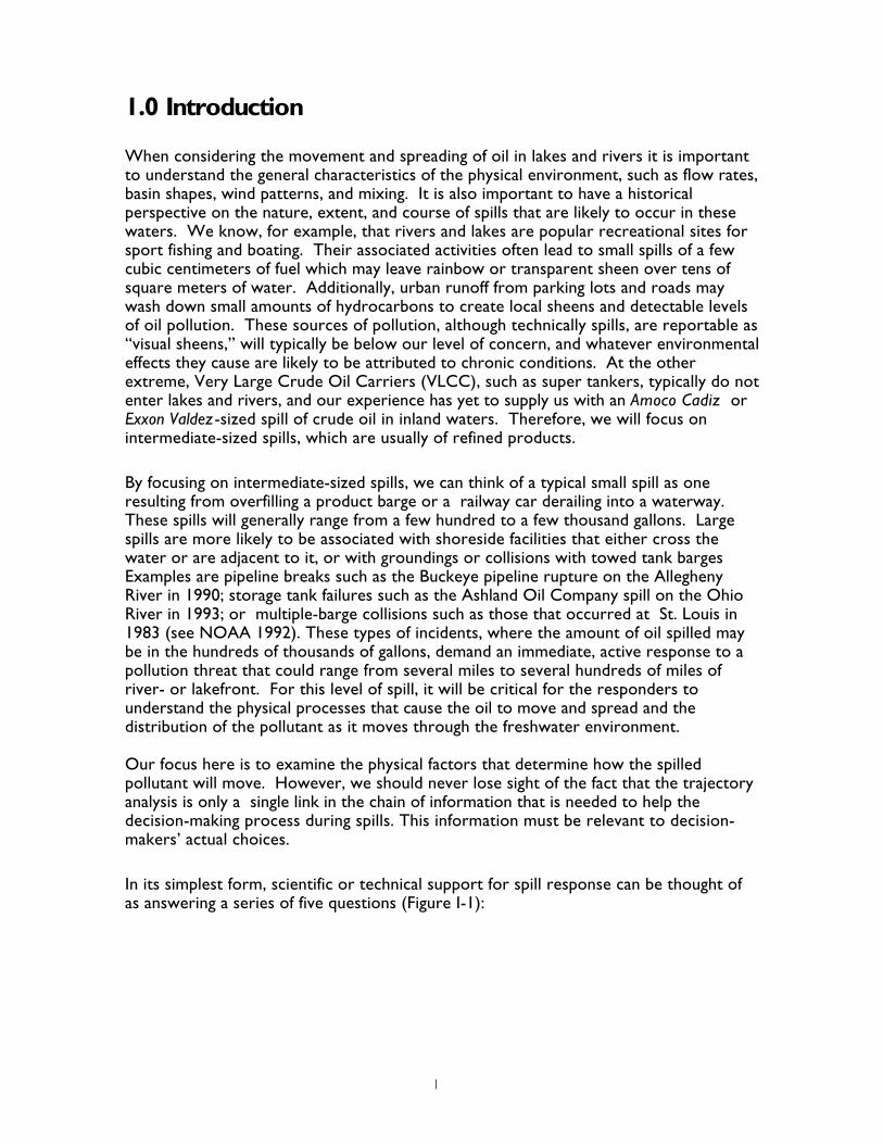
1.0 Introduction

When considering the movement and spreading of oil in lakes and rivers it is important to understand the general characteristics of the physical environment, such as flow rates, basin shapes, wind patterns, and mixing. It is also important to have a historical perspective on the nature, extent, and course of spills that are likely to occur in these waters. We know, for example, that rivers and lakes are popular recreational sites for sport fishing and boating. Their associated activities often lead to small spills of a few cubic centimeters of fuel which may leave rainbow or transparent sheen over tens of square meters of water. Additionally, urban runoff from parking lots and roads may wash down small amounts of hydrocarbons to create local sheens and detectable levels of oil pollution. These sources of pollution, although technically spills, are reportable as “visual sheens,” will typically be below our level of concern, and whatever environmental effects they cause are likely to be attributed to chronic conditions. At the other extreme, Very Large Crude Oil Carriers (VLCC), such as super tankers, typically do not enter lakes and rivers, and our experience has yet to supply us with an Amoco Cadiz or Exxon Valdez-sized spill of crude oil in inland waters. Therefore, we will focus on intermediate-sized spills, which are usually of refined products.

By focusing on intermediate-sized spills, we can think of a typical small spill as one resulting from overfilling a product barge or a railway car derailing into a waterway. These spills will generally range from a few hundred to a few thousand gallons. Large spills are more likely to be associated with shoreside facilities that either cross the water or are adjacent to it, or with groundings or collisions with towed tank barges Examples are pipeline breaks such as the Buckeye pipeline rupture on the Allegheny River in 1990; storage tank failures such as the Ashland Oil Company spill on the Ohio River in 1993; or multiple-barge collisions such as those that occurred at St. Louis in 1983 (see NOAA 1992). These types of incidents, where the amount of oil spilled may be in the hundreds of thousands of gallons, demand an immediate, active response to a pollution threat that could range from several miles to several hundreds of miles of river- or lakefront. For this level of spill, it will be critical for the responders to understand the physical processes that cause the oil to move and spread and the distribution of the pollutant as it moves through the freshwater environment.

Our focus here is to examine the physical factors that determine how the spilled pollutant will move. However, we should never lose sight of the fact that the trajectory analysis is only a single link in the chain of information that is needed to help the decision-making process during spills. This information must be relevant to decision-makers’ actual choices.

In its simplest form, scientific or technical support for spill response can be thought of as answering a series of five questions (Figure I-1):

1

What was spilled?

Where will it go?

What will it impact?

What damage will be done?

What can be done?

Figure 1-1. Steps in spill response.

First, we need information about the nature and extent of the spill. Second, we need to estimate how the pollutant will spread and what form it will take as it moves in the waterway. (Perhaps one of the key factors that distinguishes spills in water from those on land is the complex and relatively rapid mobility of the spilled material.) Third, we need to identify valuable resources (both natural and commercial) in the spill’s trajectory. Fourth, we need to understand the sensitivity of the various resources encountered to the pollutant, and the kinds of damage that might be expected. Finally, what do we do with these data? Are there any options open to responders that will make a positive difference in the outcome of the spill or that will reduce the probability that resources will be damaged?

When describing the movement and spreading of a pollutant, the physical scientist should provide analyses that are as accurate as possible. However, it is at least as important to know what the analysis does not include as it is to know what it does include. This can be exemplified by procedures used in game theory, where decisions must be made under critical, time- and data-sparse, and hence, uncertain, conditions.

In any game where chance plays a part, the players draw on all of the information available to try to achieve a “maximum win.” This would provide the best chance of maximizing the players’ return. An alternate, and generally different, game strategy might be appropriate if a player is protecting very high- value resources. In this case, the player would attempt to “minimize regret” rather than “maximize win.” Thus a decision must be made on a strategy that will make sense of the many variables associated with spills. In spill response, a “maximum win” strategy would develop a forecast using as accurate information as possible on winds, currents, and the pollutant’s initial distribution. This “best shot,” or most probable scenario, contrasts with a “minimum regret” strategy that uses a range of analysis techniques to investigate the sensitivity of various estimates to error in the data used (See, for example, Operations Analysis Study

2

Group 1977). A “minimum regret” strategy also incorporates the implications of alternate hydrological and wind conditions. For example, what is the significance of an atmospheric frontal passage six hours before the predicted time of arrival of an oil slick? What is the likelihood of a heavy rain causing a rapidly changing discharge or flash flood? The resulting analysis can provide the response organization with the “best guess” and, at the same time, cover alternate scenarios that might present a significant threat. The major difference between these two approaches is that the second one can identify less likely, but extremely dangerous or expensive, scenarios that may require the development of alternate protection strategies. These might include setting up monitoring or reconnaissance activities and identifying reserve equipment or personnel.

With these considerations in mind, we can now describe some of the physical aspects of the movement and spreading of oil spills in inland waters. We will discuss what is thought to be happening physically as well as the modeling and algorithmic approaches that are used to represent what is happening. To the extent that the computational procedures fall short of representing reality, or that the required input data may be uncertain, we must incorporate appropriate measures of uncertainty in the response advice that is generated. It is only after this process is completed that we can technically support a “minimum regret” spill response strategy.

In Section 2, we will discuss properties of oil both as it is originally shipped and as it starts to weather once it is spilled. Section 3 briefly outlines and describes the physical processes that affect the movement and spreading of oil from a hypothetical spill site to potential resources. Section 4 describes some of the more commonly used computational, or algorithmic, procedures that describe these processes. Finally, Section 5 discusses trajectory analysis procedures and modeling strategies that contribute important information to support spill response efforts.

3

This page intentionally left blank.

4

2.0 Oil Properties

2.1 General

Crude oil is the liquid component of petroleum, which also exists as petroleum gases such as propane and butane, and in a number of solid forms such as asphalt and bitumen. Any of these states can coexist, depending on the history of local geochemical processes. As discussed by (Clark and Brown 1977), crude oil is a mixture of complex organic and inorganic compounds, whose composition can vary greatly from one oil field to the next, within the same field, and even at different times and depths within the same drill hole. This variability is documented by NOAA (1994a), Environment Canada (1994), and others.

According to Clark and Brown (1977), crude oil contains somewhere between 50 to 98 percent hydrocarbons (those compounds consisting of only hydrogen and carbon atoms). The non-hydrocarbon fraction is made up mostly of organic compounds that contain nitrogen, sulfur, oxygen, and heavy metals such as nickel and vanadium. We mention these non-hydrocarbon impurities for three reasons.

First, because they are often used as descriptors of oil composition, such as “sour” as applied to crude oil having a high sulfur content. For example, Kuwait crude is considered “sour” because it has a sulfur content almost ten times that of South Louisiana crude, which is “sweet.”

Second, it is now believed that the non-hydrocarbon fraction of oil is an important ingredient in emulsification, in which large quantities of water droplets can be incorporated into spilled oil to form emulsions composed mostly of very small water droplets. Under certain chemical and turbulent energy conditions, this phenomenon can result in the formation of so-called “chocolate mousse”, a very viscous fluid having significantly different physical properties than those of the parent oil.

Third, the non-hydrocarbon fraction is generally more soluble and often more toxic than the hydrocarbon fraction. This fact is particularly important for freshwater spills, where dilution capacity might be restricted and dispersion into the water column could affect drinking and industrial water supplies. Also, in some cases, toxicity to aquatic organisms is believed to be relatively greater in fresh water than in salt water due to decreased capacity to maintain osmotic balance (Green and Trett 1987).

2.2 Classes of Petroleum

The hydrocarbon component of petroleum is a complex mixture of organic compounds which, for simplicity, can be placed into three general classes, according to their molecular structures. These three classes, which have a number of sub-classes, provide a working description of oils. The classes are:

Paraffins. These are also known as alkanes (not to be confused with alkenes). Paraffins have all carbon atoms arranged in open chains, either straight or branched.

5

They exist in gaseous, liquid, and solid or semi-solid form, such as petroleum jelly, depending on how many carbon atoms they possess (Figure 2-1). Paraffinic hydrocarbons are slightly less dense than other hydrocarbons with equal carbon atoms.

Naphthenes . These are also known as alicyclic compounds, and often have the carbon atoms arranged in one or more rings (hence the suffix -cyclic). Naphthenes resist weathering and are slightly denser than paraffins at the same boiling temperature.

Aromatics. The classical six-carbon benzene ring is the basic building block of aromatic hydrocarbons. Aromatic compounds are then composed of various combinations of linked and fused benzene rings, which are often linked to paraffinic chains. Generally, the amounts of aromatics in petroleum are relatively small compared to paraffins and naphthenes. This is fortunate since aromatics are generally considered to include compounds which can be toxic, carcinogenic, or both.

(one or more rings)

AROMATIC

HYDROCARBON COMPONENTS

< 5 carbon atoms at room temperature

gas

liquid 5 -16 carbon atoms at room temperature

solid semi-solid

> 16 carbon atoms at room temperature

(open-chain)

PARAFFINS (ALKANES)

(benzene rings)

(ALICYCLIC) NAPHTHENES

Figure 2-1. Simplified classification of petroleum hydrocarbons.

Note that oil classification does not follow a rigid scheme, as comparison of the above simplified form used by Clark and Brown (1977) with an equally simplified, but slightly

6

different, scheme used by Bobra (1990). One of Bobra's main interests has been the chemistry of water-in-oil emulsions. He and others have identified the importance of the following compounds in this process (Bobra 1990):

Waxes . The high molecular-weight paraffinic components of oil which are in crystal form when the oil is below its pour point.

Asphaltenes. Asphaltenes are non-hydrocarbons and are defined in terms of their solubilities, rather than their compositions. By definition, asphaltenes are soluble in aromatic solvents and insoluble in alkane solvents. Hence, the physical behavior of oils depends on, among other things, the ratio of the concentrations of aromatics and alkanes.

Resins. Resins are non-hydrocarbons, consisting of high-molecular weight, polar compounds containing oxygen, nitrogen, and sulfur.

These compounds are considered to be key ingredients in the emulsification process, since they provide the necessary surfactants and colloidal solid particles at the oil-water interface (Bobra 1990; Fingas et al. 1995)

2.3 Density, Specific Gravity, and °API Gravity

The density (or equivalently, specific gravity or degrees API gravity), viscosity, pour point, and distillation temperatures are the most important physical properties of petroleum. The density of a material is defined as its mass per unit volume. For, example the density of sea water is approximately 1,025 kg/m3, depending on its temperature and salinity; the density of fresh water is about 1,000 kg/m3, depending on its temperature. Specific gravity is a commonly used, non-dimensional description of density. Specific gravity is defined as the ratio of the mass of a given material to the mass of fresh water, for the same volume and at the same temperature. For example, the maximum density of fresh water is exactly 1,000 kg/m3 at 4°C. So, the specific gravity of a substance, such as oil, is exactly the same as its density relative to the density of fresh water at 4°C. Also, oil becomes slightly more dense as its temperature decreases, and vice versa.

The U.S. petroleum industry has customarily used the so-called °API (Degrees API Gravity), an arbitrarily chosen function named after the American Petroleum Institute (API) that is inversely proportional to the true specific gravity and given by

141.5° API = −131.5 , where s is the specific gravity.

s

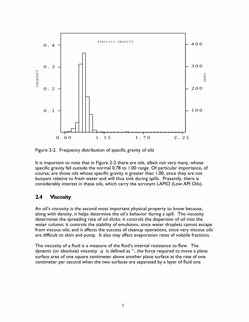
The specific gravity of most crude and refined oils lies between 0.78 and 1.00 (Clark and Brown 1979). This can also be seen in Figure 2-2, which shows a frequency distribution of specific gravity of the roughly 1,000 oils contained in the ADIOS™ oil library (NOAA 1994). Therefore, the °API gravity, as defined above, places most oils within a convenient range of 10 - 50 °API.

7

0.1

0.2

0.3

0.4

100

200

300

400

FREQUENCY COUNT

SPECIFIC GRAVITY

0.60 1.15 1.70 2.25

Figure 2-2. Frequency distribution of specific gravity of oils

It is important to note that in Figure 2-2 there are oils, albeit not very many, whose specific gravity fall outside the normal 0.78 to 1.00 range. Of particular importance, of course, are those oils whose specific gravity is greater than 1.00, since they are not buoyant relative to fresh water and will thus sink during spills. Presently, there is considerably interest in these oils, which carry the acronym LAPIO (Low API Oils).

2.4 Viscosity

An oil’s viscosity is the second most important physical property to know because, along with density, it helps determine the oil’s behavior during a spill. The viscosity determines the spreading rate of oil slicks; it controls the dispersion of oil into the water column; it controls the stability of emulsions, since water droplets cannot escape from viscous oils; and it affects the success of cleanup operations, since very viscous oils are difficult to skim and pump. It also may affect evaporation rates of volatile fractions.

The viscosity of a fluid is a measure of the fluid’s internal resistance to flow. The dynamic (or absolute) viscosity µ is defined as “...the force required to move a plane surface area of one square centimeter above another plane surface at the rate of one centimeter per second when the two surfaces are separated by a layer of fluid one

8

centimeter in thickness...” (Clark and Brown 1977). The unit of measurement of dynamic viscosity is the poise (P). For numerical convenience, the centipoise (cP) is often used and is defined as cP = 1/100 P.

It is also convenient to define an alternative, kinematic viscosity ν , which is simply the fluid’s dynamic viscosity divided by its density. The unit of measurement of kinematic viscosity is the stoke (St). Again for convenience, the centistoke (cSt) is often used and is defined as cSt = 1/100 St. Both dynamic and kinematic viscosities are used in oil spill work. Since the density of oil is not too different from that of water, rough calculations involving oil viscosity are not very sensitive, numerically, to which version is used.

Speight (1991), NOAA (1994a) and others show that the viscosity of a given oil increases with increasing density, although the relationship can be highly variable. Fresh oils and refined products have viscosities that range from less than 1 to almost 100,000 cSt (NOAA 1994a).

As in the case of oil density, discussed earlier in the section on specific gravity, oil viscosity also increases with decreasing temperature. The relative change with temperature depends on the oil. However, it appears to increase with an oil’s paraffin and hence, wax content. Viscosity increases as the oil is aged by evaporation of the lighter (low-molecular weight) components, and by photochemical and microbial processes. These and other related processes are generally known as “weathering.”

The viscosity of most fresh oils under normal temperatures exhibits what is known as “Newtonian” behavior. Recalling the previous definition of absolute (dynamic) viscosity, a fluid is considered Newtonian if its deformation, or strain, is directly proportional to the stress that is applied to it (starting from zero stress). The slope of the resulting straight line is then, by definition, the coefficient of viscosity. Oils with large concentrations of waxes or those that have been exposed to the elements (or other conditions that could increase their viscosity) may behave more like a visco-elastic or plastic material. These types of product exhibit complex flow behavior known as non-Newtonian, which influences the spreading and vertical dispersion of spilled oil and, by extension, the efficacy of cleanup methods (for example, the use of shovels vs. pumps). Table 2-1 gives a general feel for the range of oil viscosities encountered in terms of more familiar substances. As a rough rule of thumb, oil can be considered non-Newtonian at viscosities above about 100,000 cP. Recently, Berger and Mackay (1994) have discussed the important behavior of high-viscosity oils on evaporation.

9

Table 2-1. General range of oil viscosities at room temperature in terms of familiar substances (Bourne 1982; Weast 1988; NOAA 1994a).

Liquid Viscosity (cP)

Water 1

Diesel fuel 10

Light machine oil or olive oil 100

Glycerin or castor oil 1,000

Honey 10,000

Molasses 100,000

Sucrose (cane sugar) 1,000,000

2.5 Pour Point

Pour point is the temperature below which an oil cannot be poured. The pour point is a property whose value is determined by methods defined by the American Society for Testing and Materials (ASTM). Clark and Brown (1977) note that the pour point corresponds to the temperature at which an oil’s kinematic viscosity is about 300,000 cSt. This is particularly useful information in colder climates, where knowing whether oil is fluid enough to be pumped without special heating equipment, for example, would certainly affect cleanup and salvage decisions. Perry et al. (1984) report pour point ranges in refined fuels of -60°C for jet fuels to +46°C for waxy No. 6 fuel oils. The spill from the motor vessel Presidente Rivera into the Delaware River in 1989 is a good example of the latter (NOAA 1992). In this case, the pour point of the product was greater that the temperature of the water, so that the spilled oil congealed into tar-like globules in which 90% of the oil was not visible from the surface. In general, however, the concept of pour point should be used with care when applied to real oil spilled on water, because of the inherent difference between conditions in the laboratory and in actual spill conditions. Also, laboratory measurements of pour point can be highly variable, since it involves the crystallization of waxy oil components. This can result in a liquid/solid mixture whose kinematic viscosity is some undetermined combination of the viscosity of the two phases (Clark and Brown 1977).

2.6 Distillation Temperature

Information on oil properties, including viscosity and specific gravity, is equally important for understanding the behavior of both crude and refined oil. However, many accidents involve refined oils of one type or another, especially in freshwater environments. Since liquid petroleum itself is not a very useful product in its raw state and since many accidents involve refined products of one type or another, the remainder of the discussion will deal mostly with refined products. Refineries use fractional distillation to extract and separate the various hydrocarbon components of petroleum. The crude

10

petroleum can be a mixture of components ranging from gases such as methane to heavy substances such as bitumen. As mentioned earlier, crude petroleum contains many impurities, such as sulfur. Impurities are often chemically removed to the extent practicable, depending on the intended use of the final product.

The boiling temperature of the material in distillation columns continuously increases as the distillates are removed. The distillates are then collected according to a range of boiling temperatures. These products are often refined again separately to produce finer “cuts.” The final distillates are then blended according to desired properties and used commercially. Fuels from American refineries are then named No. 1 - No. 6, as defined by ASTM (see Perry et al. 1984).

Fractional distillation is a process in which the more volatile components of petroleum boil away, leaving a residuum. Therefore, both the density and the viscosity of the refined oils should increase with boiling range. Figure 2-3 shows this expected relationship, including ranges of density and viscosity.

Figure 2-3. Viscosity, boiling range, and specific gravity for typical fuel oils (adapted from Perry et al. 1984).

Figure 2-4 shows a viscosity-temperature relationship for common fuels, including guidance for maximum viscosity for storage, pumping, and handling. Properties of the oils shown in Figures 2-4 and 2.4 are discussed in more detail by Curl and O’Donnell (1977) and Clark and Brown (1977). No. 2 fuel oil (diesel) and No. 6 fuel oil (Bunker C) have been chosen by the American Petroleum Institute (API) as reference oils representing light and heavy refined products, respectively. (Similarly, API has designated Prudhoe Bay and South Louisiana as reference crude oils.)

11

Figure 2-4. Kinematic viscosity as a function of temperature for typical fuel oils (adapted from Perry et al. 1984).

Clark and Brown (1977) note that a typical No. 2 fuel oil contains roughly 30% paraffins, 45% napththenes, and 25% aromatics; while a Bunker C fuel oil contains about 15% paraffins, 45% napththenes, and 25% aromatics. The remaining 15% is made up of non-hydrocarbons.

2.7 Flash Point

Drysdale (1985), who discusses the flash point of combustible liquids in some detail, defines it succinctly as “...the lowest temperature of the liquid at which the vapor/air mixture will ignite...” The flash point of combustible liquids is inversely proportional to their equilibrium vapor pressure, so that such liquids are often classified according to flash point, which can be used as an index of hazard: the lower the flash point, the greater the hazard. The flash point of an oil, a mixture of many components, can be estimated by using Raoult’s law and the vapor pressures of its main components. The flash point could be an important consideration in operations such as in-situ burning of large spills, or in accidental fires involving large amounts of oil collected in restricted areas of rivers and embayments.

12

2.8 Emulsification

As mentioned earlier, many oils form long-lived emulsions when water droplets are incorporated into oil. This “chocolate mousse” can contain as much as 80 % water and can be extremely stable with respect to water removal. Studies by Bobra (1990) and others have shown that emulsification occurs in oils with relatively high asphaltenecontents. Moreover, many laboratory experiments and casual observations attest to the fact that high-energy environments enhance emulsification. However, the understanding of the chemical and physical processes leading to this phenomenon is still so poor that, in most cases, mathematical models cannot reliably predict emulsion formation. Nonetheless, most oil-weathering models include an algorithm for mousse formation that may be invoked, depending on the user’s confidence in the algorithm or his/her ability to use it, to calculate an answer judged to be reasonable.

Assuming that an oil can form an emulsion chemically, it has been shown that the emulsification rate is proportional to the intensity of the water turbulence (Wang and Huang 1979; Mackay et al. 1980; Fingas et al. 1995). Also, it appears that emulsification, once started, proceeds quite rapidly. Mackay et al. (1980) have proposed a simple first-order rate law for mousse formation. This and similar formulations have been discussed by Payne 1985.

Not only do emulsification and evaporation change the physical properties of the material in a slick, and thus, perhaps, the type of response necessary, but they also increase the volume of the material to be dealt with in the response, as in the case of the Exxon Valdez spill (NOAA 1992)

13

This page intentionally left blank.

14

3.0 Transport Processes

3.1 General

When considering transport processes in inland waters, it might appear that the problems are less complex than what we would expect to encounter in oceans and estuaries. For example, in rivers the flow is generally in one direction and lakes typically have quite weak currents. In some ways, these simplifications are true, but the actual details are more complicated. To understand oil spill trajectory analysis in inland waters it is important to review the resources to be protected. Then we can consider the transport mechanisms that might move the oil in such a way as to threaten these high-value resources.

In marine oil spills, it is very unusual to consider the water itself as a resource to be protected. Spilled oil may move over or through the water, but the water itself is not generally thought to be damaged. For inland spills this is not true. In most cases, the water is used as a primary resource (potable water) and threats to the water supply are a public health problem, immediately escalating the level of concern in inland spills. The movement of oil toward drinking-water intakes is a critical trajectory analysis problem. Time of first arrival and duration of the threat need to be known so that emergency measures, such as filling storage facilities, drawing from backup wells, processing shutdown, and rationing, can all be planned in the least disruptive manner. Beyond drinking water supplies, power-plant intakes that use water as a coolant and industrial processing intakes are often threatened by potential degradation of water quality. Questions related to these intake points will typically follow the public-health issues.

For most inland water spills the shoreline is threatened with pollution almost at once and the prospect of large-scale dissipation of oil, as at sea, is not even a remote possibility. As in marine spills, the nature of the shoreline will determine the amount of potential damage that a spill could cause. For example, steep or manmade shores will probably not sustain long-term impacts while marsh and wetland areas will be significantly threatened by oil impacts. Inland waters have insignificant tides (except for possible upstream approaches to estuaries); the segment of shoreline actually threatened by oiling tends to be smaller than would a marine intertidal area shoreline. However, irregular, longer-term changes in water level can have some influence. For example, flooding can strand pollution at high levels and threaten larger areas than might otherwise be expected. Flooding also occurs in large, relatively shallow lakes, most notably Lake Erie, which is well-known for its rapid response to extra-tropical storms. Strong winds and changes in atmospheric pressure can produce seiches and lake setup to the extent that the lake’s surface elevation may vary by more than a meter between the two ends of the lake.

Inland waters have an enormous recreational potential. Moreover, large numbers of people place value on the aesthetic appeal and use these waters as a destination for fishing, camping or swimming. Oil pollution events seriously degrade the recreational value of the areas and thus become a serious cleanup issue.

15

When a spill occurs in inland waters there are a number of technical issues that need to be considered. To understand these issues it will be necessary to first answer some questions about the physical processes that affect the movement and spreading of the oil. At a minimum, there are three problems that will present themselves in nearly all inland spills. These problems involve:

1. Predicting the travel time of the leading edge of the pollutant plume and the duration of the plume’s passage for points (typically water intakes) along rivers and lake shores;

2. Identifying shoreline areas where oil is likely to strand or accumulate; and

3. Estimating the residence time for objectionable concentrations of floating or suspended oil in high-use areas.

3.2 Flow in Rivers

The spill response community has a great deal of experience in ocean and estuarine environments compared with experience with rivers. At first, it might seem that at least the physical processes portions of this experience could simply be applied to rivers as though they were oceans or bays. This is a bit misleading even when we account for the changes in shoreline shape and current direction, because of the fundamental difference in the turbulence levels and current shears typical in rivers. In oceans or large lakes, surface-wave activity is the major source of turbulence. Because of this, turbulence levels typically drop off with depth. Although floating pollutants may be mixed into the water column by breaking waves, they usually refloat and concentrations remain essentially a two-dimensional distribution.

In contrast, shear in currents along the river bottom and banks are typically the major source of turbulence. Thus, mixing and dispersion caused by the interaction of the shear and the turbulence can move significant amounts of oil below the surface (particularly if it is relatively dense, such as a heavy No. 6; or if it is finely distributed as droplets). The shear-dominated river regimes tend to produce spill distributions having higher subsurface oil concentrations than would be expected in marine spills.

Shear-dominated flows cause another effect that characterizes river spills. The lower speeds along the banks and bottom of a river indicate that the surface and center of a river move downstream faster than the flow along its boundaries. Therefore, mixing will continuously exchange water and pollutants between the slower, near-bank regions and the faster, center regions of the river, with the resulting smearing of the distribution along the axis of the flow. More specifically, some patches of the pollutant will move out of the mainstream, slow down, then return to the main flow somewhat behind their initial location. This difference in current speed is typically the major mixing mechanism that spreads a pollutant patch out as it moves down a river. As a result, it controls the shape and size of a plume and the distance over which a pollutant concentration will remain above a particular level of concern. The response to a given size spill is then largely controlled by the details of the shear in the channel’s flow.

16

A second consequence of shear-dominated flow is that, although the leading edge of the pollutant distribution may move as a relatively sharp front (at the current speed in the middle of the channel), the tail end of the distribution is continually mixed and smeared. Therefore, the actual pollutant distribution will begin to resemble a comet, i.e. with a relatively distinct front followed by a fuzzy tail. This “holdup” in rivers due to “dead spots” in the flow are discussed by Fischer et al. (1979) and others. From a practical point of view this means that, although it might be possible to predict the initial arrival of a pollutant at an intake point along the river, it will be considerably more difficult to estimate when the threat is past, since the slower areas in the river are continually supplying pollutant to the main stream, even after the “comet’s” head is past. For example, the first arrival time (shut-down schedule) could be estimated by a simple calculation that divides the discharge data from the river by the cross-sectional area and integrates the resulting velocity displacements along the channel. However, this method would tell the responder nothing about the distribution at any particular point, nor would it tell municipal authorities when it is safe to reopen water intakes.

On a long, straight channel the flow is unidirectional. Small-scale mixing across shear boundaries is the major mechanism for moving pollutants across the river. However, few natural channels are actually straight, and it is necessary to consider the effects of shoals and, particularly, bends in rivers. As water moves around the bend in a river, centrifugal force tends to pile water up along the outside edge of the turn. This causes a pressure gradient directed toward the inside of the turn that is just sufficient to actually accelerate the water around the bend. Since water does not leave the channel, it must be that the pressure gradient at the surface must just balance the velocity- dependent centrifugal force. Near the bottom of the river, the velocity decreases due to friction. Therefore the centrifugal force is smaller and no longer balances the pressure gradient force. This unbalanced pressure force causes a secondary flow that moves water along the bottom toward the inside of the river bend. To conserve water there must be a weak return flow toward the other side of the river bend throughout the water column (above the bottom friction layer). This secondary flow, when superimposed on the normal, and usually much stronger, down-channel flow produces a slow, helical motion as shown in Figure 3-1. Its effect can be seen in older river channels where the flow tends to deposit bottom silt and sediments along the inside of river bends with stronger currents along the outer bank of the turns.

Figure 3-1. Cross-section of a meandering stream showing secondary flow.

17

This leads to the meander patterns seen across the flood plains of mature rivers as shown in Figure 3-2.

Figure 3-2. Flow in a meandering river.

From a pollution distribution point of view, the secondary flow slightly deflects the streamlines in the flow as the river moves around bends. More significantly, secondary flow helps move oil particles across the shear boundaries and greatly increases the smearing, or dispersion, of the pollutant patch in the downstream direction. Thus pollutants tend to spread more rapidly, decreasing their peak concentrations relative to what would be expected for a straight channel.

Many river cross-channel profiles are very irregular, with rapids at one extreme and bays at the other. These features either accelerate or decelerate the average flow down the river. It is also clear that these irregularities will cause pollutant distributions to speed up or slow down and contribute to the shear in the current pattern. In trajectory analysis, such features require us to modify time-of-travel estimates to predict first arrivals. We should expect that these differences will significantly increase the along-channel spreading of the pollutant distribution.

3.3 Modification to River Flow by Structures

Rivers that are likely to be used to transport large volumes of hydrocarbons are, by definition, navigable. As such, they will usually have engineering modifications. Typical examples would be the jetty and flow restrictors that are common along some sections of the Mississippi River or the lock and dam systems that are seen in the Ohio and Columbia rivers.

18

Flow restrictors are intended to control sediment migration in navigation channels and to maintain current velocities to avoid excessive silt buildup. While accomplishing these objectives, they also introduce artificial side bays that may have recirculation eddies and backwaters, where the flow may even move upstream temporarily. These flow features can change the shear patterns in the current and often provide convergent traps where floating pollutants accumulate. These areas may be natural collection points where impacts are likely and cleanup and recovery options may be necessary.

Lock and dam systems control the river’s slope, reduce velocities, and provide sufficient water depth to maintain navigation channels. Each lock position has a spillway to drop excess volume flow. These structures are usually dams with either overflow weirs or underflow channels (sluice gates). In either case, the drop in potential energy causes turbulence that is distributed throughout the water column, so that any pollutant that passes through them is rapidly mixed from top to bottom (Figure 3-3). The speed with which a floating pollutant refloats and appears at the surface will depend on its particle or droplet size and its relative buoyancy. For example, during the Ashland oil spill the No. 2 (diesel) fuel oil that overflowed dam spillways typically took a number of kilometers before its distributed droplets returned to the surface and coalesced into a continuous, recognizable slick. NOAA (1994b) and NOAA and the American Petroleum Institute (1994) discuss response options in cases where the natural flow is interrupted by flow-control structures.

Figure 3-3. Vertical mixing in the tail waters of an overflow dam.

There is a striking difference in the ways overflow and underflow dams affect a floating pollutant. Overflow dams will take the shallow sheet of water and pollutant at the surface and plunge it into a full-depth mixing zone on the downstream side of the dam. This is extremely effective in achieving a well-mixed distribution. Just downstream from such dams we would expect to find the highest concentrations of oil distributed in the water itself and, subsequently, the greatest threat to subsurface water intakes. On the other hand, sluice gates usually discharge near the base of dams, so that they tend to

19

restrict the discharge of floating pollutants and, in this respect, make fairly effective booms. As such, these are areas where virtually all floating material accumulates, making them good oil collection and recovery points. However, there are often large amounts of other flotsam that present an extensive oiled waste and disposal problem. If the flow through dams using sluice gates exceed about a knot, oil that accumulates behind them will then be entrained through the system. The dam’s booming characteristics will thus fail to stop the oil, just as any boom would fail under these conditions.

3.4 Lake Circulation Currents within lakes are usually relatively weak except during periods of strong winds or relaxation from storm events, which must be considered as special events. The flow associated with the inflow from rivers and the drainage into other rivers is usually weak except quite close to river mouths. From a floating-pollutant point of view, there is a significant difference between these relatively small inflow and outflow regimes. Where water enters a lake, the currents spread both horizontally and vertically and thus show a marked deceleration. This is accompanied by strong, localized surface convergences that tend to collect floating material. The velocity fan formed as the river enters a lake is a natural collection point for oil coming down the river, which may be useful during a response. In contrast, the outflow from a lake into a river creates an acceleration zone where floating oil is likely to accumulate. Response schemes for both input and outflow areas are discussed by Breuel (1981).

Wind-driven flow in lakes forces the water downwind until the resulting pressure gradient (retarded by bottom friction) forces a return flow. This behavior is controlled by the geometry of the lake and the time dependence of the wind, and may result in complex current patterns. If the wind blows long enough, water will move downwind in the shallow regions and set up a return flow in the deeper regions of the lake. Since a net mass balance is required, the downwind currents in the shallow regions are stronger than the return flows where it is deep. This is a major simplification of wind-driven flow in lakes, but the details are case-specific. Typically, computer simulations are used to generate current patterns, as described in Section 4.

Strong weather events can cause large lakes to behave like inland seas. Circulation patterns will have to be closed, but within a local area, such as along a particular shoreline, relatively strong coastal currents can develop. In addition, fast-moving storms may cause significant surges that cause oscillations in the currents and may change the position of the shoreline. This will be a significant factor in wetlands along the edges of large lakes. From a pollutant response point of view, the trajectory problem becomes significantly more difficult under these circumstances. Oil can be stranded on shorelines or submerged by the return to normal lake levels. The potential difficulties and uncertainty associated with these events must be factored into trajectory analysis procedures.

3.5 Wind and Wave Effects

The effect of wind and waves on inland oil spills differs, depending on whether the spill is in a river or in a lake. In rivers, the currents tend to be strong with a relatively small

20

fetch over the water. Wind and wave effects are thus usually of secondary importance. Thus, for river spills, the currents and shear dominate the distribution processes with the wind acting in a minor way to determine which bank of the river the spill will trend toward. It may be of interest to point out that many large rivers act as state boundaries so that the wind, although secondary in the actual movement of the oil, may determine which state the pollutant landfalls are located and thus change the jurisdiction of the major concerns. Unlike rivers, lake currents tend to be small. In lakes, wind and wave factors typically dominate the distribution processes, both directly and indirectly by the wind-induced currents. Waves affect the movement and spreading of oil spills in several different ways, and the relative importance of these processes change as the pollutant weathers. Initially, as the oil spreads to form a thin film, short-gravity waves are absorbed by the film, forming an oil “slick.” The slick appears smooth compared to the oil around it. The thinnest transparent films are really only distinguishable by this change in surface roughness, and can be likened to looking at the difference between silk and corduroy materials. In any case, as these waves are absorbed by the oil film, momentum is transferred from the waves to the film. This has several effects.

First, small waves approaching from a dominant direction tend to push oil slicks in the direction of wave propagation, so that floating oil films move slightly faster than the surface of the water that they are floating on. This differential oil-water velocity has been measured a number of times at spills and ranges between 0.7% and 1.4% of the observed wind speed (Galt 1994). Note that, although this depends on the waves, it also correlates reasonably well with the wind, since it is the wind that generates these small waves in the first place. This wave/oil-film interaction will tend to be significant as long as the oil continues to form a slick. It will be reduced somewhat as the oil breaks into streaks and streamers. As the oil weathers and forms tarballs, this wave stress and momentum transfer becomes negligible.

A second transport mechanism associated with waves is the current generated by short, relatively steep waves. This so-called “Stokes drift” results in a surface current that will move the oil in the dominant wave direction, which again is downwind.

A third process associated with waves is vertical dispersion, which has already been mentioned. This process is related to the turbulence created by the waves and thus depends less on the general wave field than on that fraction of the waves that are breaking. As waves break, the resulting plunging water creates turbulent wake, carrying particles of oil down into the water column. Some of the particles are so small that their rate of refloating is essentially zero, and they are permanently “dispersed” in the water column. For larger particles these excursions below the surface are usually temporary and, due to the oil's buoyancy, can be considered as only spending some fraction of their time away from the surface. As mentioned in Section 2, oil is less buoyant in fresh water than in sea water, so the submergence time of these oil droplets is relatively greater in fresh-water than in marine spills.

Another phenomenon often observed in turbulent conditions is so-called “overwashing,” where oil particles or tarballs can be driven some distance below the surface. As larger fractions of the oil particles are below the surface, the actual spill

21

becomes progressively more difficult to observe from the air. Under these conditions, it is not uncommon for reconnaissance flights to report that the spill has dissipated, only to find that it seems to have returned when the weather improves and the sea state decreases. This “disappearing act” and the fact that, from a boat, it is often possible to observe a tarball below the surface, have led to reports that the oil is sinking at nearly every major spill. During the 1979 IXTOC I spill in the Gulf of Mexico, divers collected information on the subsurface distribution of tarballs. Strong wind conditions drive the tarballs deeper into the water; quiet conditions allow them to move back toward the water surface. In fresh-water spills this “disappearing act” could be even more pronounced. It appears that oil sinks in the same way that dead leaves fly from the ground. Actual sinking, in the sense that oil is permanently removed from the surface, only occurs if (1) the oil is denser than the surrounding water, (2) the buoyant rise of very small oil droplets will be impeded by friction of the water; or (3) if the oil has been mixed with enough sediment .

It is commonly understood that wind significantly affects the movement and spreading of oil spills. However, the effects are not direct, but rather occur through other processes that the winds cause, which in turn affect the movement of the pollutant. The wave processes mentioned above are examples of this indirect wind forcing. As was seen, it is not the wind that is interacting with the oil, but rather the waves which, in turn, are well correlated with the observed winds. Therefore, from an algorithmic point of view, the winds become one of the primary prediction parameters.

In addition to forming waves, wind stress drives a number of complex surface currents that will also contribute to the movement of floating oil. The actual dynamic processes of how the wind moves the water are very involved and require extensive, non-linear analysis to develop a reasonably complete theory. Fortunately, for the purposes of trajectory analysis it is sufficient to use simple theories to describe the processes that we cannot technically predict.

The movement of water in a thin surface layer is the primary current directly caused by the wind. In the original theories describing this current, the flow direction was at 45 degrees to the right of the wind, in the northern hemisphere. A more detailed analysis suggests that the deflection angle is considerably less than that and is more likely to be in the ten-degree or less range. As a practical response algorithm, it is usually adequate to simply assume a wind-driven surface current having a velocity that is about two percent of the wind speed and in approximately the same direction as the wind. However, it is important to recognize that these quantities are rough averages obtained from different experiments, at different places and times and variability can be large, as shown by Brown (1991) and others. Also, it should be remembered that, when predicted winds are being used for trajectory analysis, they are typically only specified by quadrant direction, so that errors associated with a few degrees are thus usually not significant for practical purposes.

The two-percent wind drift rule is a reasonably good approximation to the primary wind-driven flow, but a closer look shows that the actual flow is unstable and tends to break up into more complex patterns called “Langmuir cells.” These phenomena begin

22

to appear if the wind becomes stronger than a few knots. Their structure is characterized by a series of counter-rotating vortices, whose axes are approximately parallel the wind direction. Convergence lines form within adjacent pairs of cells and divergence zones form between pairs of cells, as shown in Figure 3-4. In a sense, the surface current moves in the direction of a series of alternating right- and left-handed corkscrews lying in the surface and pointing in the direction of the wind. The distance between adjacent corkscrews, or convergence lines, varies from a few meters to tens of meters. Obviously, the surface flow is still generally downwind, but much more complex in detail. Langmuir cells, which are ubiquitous in the ocean and in lakes, are believed to form as a result of a complex interaction between surface currents and surface waves. They are considered to be a major mechanism for the exchange of atmospheric gases and other material at the water surface. In particular, the convergence lines are easily visible as band-like water slicks, or more importantly as sites of floating debris. It is important to note the asymmetry in cell spacing, which indicates that the downward velocities in the convergence zones are greater than the upward velocities in the divergence zones. It is known that Langmuir circulation in the presence of waves is an important mechanism for aeration of surface waters by injection small air bubbles. Dispersed oil droplets and air bubbles are comparable in size and behavior, and it is possible that Langmuir circulation provides an efficient pathway for vertical transport of oil from the surface (Thorpe 1984; Zedel and Farmer 1991; Farmer and Li 1994).

Figure 3-4. Simplified Langmuir cells showing flotsam at surface convergences.

A floating oil film will be affected by Langmuir cells and will tend to thicken and collect in the convergence bands. Between the convergence bands where the surface flow is diverging, the oil film may rupture and form a banded gap. Together, it is likely that Langmuir cells will cause a distribution of floating oil that is banded, or in streaks and streamers oriented in the direction of the wind. Under strong wind conditions, oil slicks rupture and become banded quite quickly, often within minutes, depending on the type of oil and the size of the spill.

From a cleanup point of view, there are some significant implications of floating oil distributions that break up into streaks and streamers under the influence of Langmuir

23

circulation. It is often thought that oil spills form a more or less continuous layer of oil but this is not true once oil breaks into streaks and streamers.

Over any particular region, the major portions of the oil may only cover a relatively small fraction of the actual water surface. Guidelines for many cleanup procedures, such as chemical dispersants, suggest that they be applied at rates correlated with the thickness of the oil and the area covered. Once the oil slick has broken into bands or streaks it is not at all clear what area the oil covers; any spray application will certainly be treating primarily open water. This fractional surface coverage is also significant for any remote sensing attempts to observe oil. The oil may extend as streaks and bands over a very large area, so that the sensor is actually looking mostly at open water, and returning a weak or ambiguous signal.

3.6 Oil Spills in Ice

In northern areas, ice can complicate and modify the movement and spreading of floating pollutants. Oil spilled under a solid ice sheet tends to form a lens that may remain relatively thick. With currents the lens can move along the underside of the ice and present a particularly complex problem. Oil under broken ice behaves quite differently: the oil floats up in the small water channels between the pieces of ice and may spread over larger areas (Yapa et al. 1993). In this case, however, the oil tends to move with the ice. In several winter spills in the Hudson River shore-fast ice in the coves and small bays acted as booms that confined the oil to the center of the channel. This natural booming protected shorelines in these areas from oiling and reduced the along-channel mixing that would be expected from the normal river shear produced by these low-current regions.

There is a second significant physical process associated with ice and oil spills. Oil pooled under a thin layer of ice while active freezing is increasing the thickness of the ice can be frozen into the plate of ice and held there until the ice melts. During the Ashland oil spill on the Ohio River, a sudden drop in temperature just after the spill produced this type of situation. Samples of ice collected along the river showed numerous examples of globules of oil frozen within the plates. A rough estimate of the area involved and the percent coverage of ice suggested that as much as 20% of the oil that reached the river might have been incorporated into the ice at one time or another. From a spill response point of view, this means that some fraction of the spill may seem to disappear only to return as the weather moderates.

Is should be pointed out that many of the important processes discussed in this section are not amenable to mathematical modeling. For example, in lakes, where surface wind is very important, Langmuir circulation, as previously mentioned, is thought to be the major factor in the production of streamers and streaks of spilled oil in the absence of density fronts. However, there are no well-established models that can predict the generation and dissipation of Langmuir cells. The latest theory on this phenomenon is that they are always present in a statistical sense, but are ephemeral as individual cells. This then presents a daunting prospect for modeling them, since they appear to be closer to small-scale, near-surface turbulence than to organized motion, even though their structure is clearly organized. The importance of scale to this, and similar types of motion, are discussed further in Section 4.

24

3.7 Special Considerations

Some processes that take place in inland waters are dominated by seasonal or episodic changes in runoff and rainfall. Some of the easiest of these changes to observe are the changes in water level and increases in river speed in response to rains. Many rivers have correlation tables that relate the river gauge height to volume discharge (rating curves). These tables can be used to estimate the average channel velocity. Whenever estimates of spill trajectories are needed on such rivers it is always necessary to compare the estimated river flow with their nominal values. Regional river forecast offices of the National Weather Service or Army Corps of Engineers operations are often a good place to obtain such information (see Appendix A for listing of NOAA River Forecast offices)

These runoff variations also change the water level, stranding pollutants on the shoreline at different levels. For example, falling water levels may strand oil so that it will not refloat, which removes it as a secondary source for a new spill, but may leave a persistent shoreline cleanup problem. On the other hand, rising water levels may wash off beached oil and reintroduce floating pollution, or they may cover up oil that is adhered to sediment or vegetation.

Changes in water level can be very important in the manmade inland water bodies and can even change the nature of the drainage system. In arid regions of the West, catchment dams will form large lakes during periods of abundant rainfall, which usually return to rivers during droughts. Parts of Lake Shasta in California and some of the dam systems on the upper Missouri River are good examples of this. At the other extreme, when discharge rates are high, some lock and dam systems behave like a river with a series of waterfalls. However, they may end up more like a series of slightly connected lakes when the flow drops off. Sections of the upper Ohio and Mississippi rivers are good examples. Under these situations, historical data collected under alternate flow conditions may be very misleading. Special care must be taken when developing estimates of movement and arrival times.

Floods are perhaps the most extreme form of water level change and introduce a whole new set of problems to trajectory analysis efforts. Some waterways do not even appear to be in the same area as they were before the flood. Numerous side lakes develop and, obviously, any models or algorithmic solutions based on normal river location or dynamics may be irrelevant. Flood conditions place much stress on the normal infrastructure of communities by cutting roads, communications, and dislocating populations. Planners must be aware that, under these conditions, spill response will be difficult and more than likely not authorities’ highest priority. In addition, it is possible that flood conditions will threaten riverside facilities and may destabilize structures enough to cause spills, exacerbating an already difficult situation.

25

26

4.0 Modeling Techniques

4.1 General

Oil spill trajectory models vary greatly in complexity and, at times, in their practical utility. Suitable models depend on many important factors, such as shape, bathymetry, and sedimentology of the water body; relative importance of forcing functions, such as winds, runoff, and local hydrography; the chemical characteristics of the spilled product; and the ease of use and accuracy of the chosen model. It is very important to remember that any model simplifies reality and that a mathematical model is only one of a number of types of models , including one’s own intuition.

The formulation of the complete set of hydrodynamic equations is well known. The solution of the equations is quite another matter. The key to successfully using mathematical models depends on the modeler’s ability to make prudent simplifications of these equations that still retain the essential features of the problem. Ideally, model users should understand the assumptions of the model and should immediately become suspicious when these assumptions are violated. Computer models should be considered as an important, but not the only, analytical tool available, and their output should never replace experience and common sense.

In most cases, the ideal model user is the model developer. This is especially true for complex models requiring large amounts of input data. This is also true for models whose computational idiosyncrasies are unfamiliar to the inexperienced, and for models that sometimes must operate on the edges of their domains of validity. However, it is clearly impractical for models to be restricted to the use of their developers only. This problem is partially solved by the modern, widespread use of menu-driven models, which not only make data entry much easier but also reduce errors by flagging improbable values, based on the modeler’s experience.

For their practical use in emergencies, complex geophysical-scale models are faced with two fundamental problems. First, the combination of their mobilization time and computing time could be excessive, depending on the circumstances. Second, the quality of the input data is often not high enough to warrant the time and expense involved in the use of complex models, whose output might be no more reliable than that of simpler models requiring fewer uncertain input data. However, in some cases, contingency planning for fixed facilities or critically sensitive areas might also include a considerable collection of environmental data that would be useful input to more complex models.

In general, the prediction of pollutant trajectories in water bodies can be thought of as a three-part process:

First, the best estimate possible should be made of the location, time of spill, and magnitude of the source.

Second, the temporal and spatial distribution of water motion must be determined, since this will determine the trajectory of the main body of the pollutant.

27

Third, the spread of the pollutant about its center of mass must be found.

Analyses based on these three processes are carried out simultaneously, and often by iteration, since model input data are often incomplete, inaccurate, or subject to change during the course of the response. The location and (potential) magnitude of the source can often be used to gauge the urgency and the type of response required. However, once the decision has been made that trajectories are required, then the determination of the flow field is the most important ingredient in the analysis. Turbulent mixing and dilution is certainly important; however, since the turbulence itself depends on the structure of the main currents, the determination of the latter is essential.

The pollutant is considered to be a scalar quantity satisfying an equation that expresses a balance between the observed time rate of change in concentration at a point with its change due to its movement by currents; turbulence; addition of material by sources; and the rate of removal of material by such processes as evaporation, sediment adsorption, and photo-oxidation.

As mentioned earlier, there is a large gap between formulating an advection-diffusion problem completely and solving it. A good feel for the scale of the problem and the use averaging over space and time are the two most effective methods available to reduce the complexity of the original problem into a more manageable form.

4.2 Scaling

In formal scale analysis, estimates are made of the relative magnitudes of each term in the equations that express the conservation of mass, momentum, and energy. This comparison is made on the basis of so-called “characteristic values” of variables, such as water velocity, breadth and depth of basin in question, effects of the earth’s rotation (Coriolis effect), and other parameters. In this procedure, the model equations are manipulated in such a way that the variables of interest are made dimensionless and of a magnitude of about one, or O(1). Comparison of the magnitude of terms in a particular equation is then governed by the relative magnitudes of dimensionless groups of multiplicative constants made up of “characteristic values” of the variables. For instance, the characteristic time in estuary problems is often chosen to be the period of the largest tidal constituent, since many estuaries’ behavior is governed by tides (similarly, a problem in one of the Great Lakes might use the seiche period as a natural time scale). The characteristic length in some river problems could be the average depth, since depth is part of most formulations for turbulent dispersion. Such heuristic arguments often allow a rough estimate of the relative sizes of all the terms in a particular equation; only the largest terms in the equation are retained to form a simpler system. In some cases, a surprising number of terms in the original equations are not very important in the “big picture” and can simply be dropped in favor of those that describe the main features of the problem at hand.

Fischer et al. (1977) discuss the importance of this "order-of-magnitude" analysis as a means of getting a feel for the scope of a problem. It is important to realize that some form of scale analysis is almost always done, either on paper or by use of intuition or

28

experience. As a typical example; sometimes Coriolis force is important in oil spill problems, and sometimes it is not. Formal scale analysis, while possibly tedious at times, usually gives criteria for guidance. On the other hand, one’s intuition, rather than mathematics, would say that Coriolis force should not play much of a role in spills on small lakes and reservoirs, simply because the body of water involved is too small for Coriolis force to cause any appreciable deflection of moving water (and hence pollutants). In marine waters or in the Great Lakes, on the other hand, where spatial scales can be larger, the Coriolis force can produce very important effects and thus generally cannot be ignored. In the case of ordinary rivers, for instance, most models ignore Coriolis effects, again because of lateral constraints. However, such effects can clearly be seen after many rivers have widened into larger-scale estuaries. Then, freshwater discharge favors the right hand side of most estuaries (looking downstream in the northern hemisphere, and vice versa), with the core of the saltwater intrusion on the opposite side.

4.3 Averaging

The fewer the places where model equations are averaged in time or space, the greater the computational requirements. This can easily make the difference between the use of a personal computer (or even a hand calculator) and a sophisticated mainframe computer. Time averages are used to remove the effects of phenomena whose characteristic time scales are shorter than the time scale of interest. A similar analogy can be used for spatial averaging. Two-dimensional circulation models are much cheaper and easier to use than three-dimensional models.

An extremely important point to notice is that, when taking averages, everything with scales smaller than the chosen averaging scale is considered turbulence, and hence not predictable with the model in question. A practical example of the effects of averaging on the accuracy of spill response, could be the use of a “steady-state” (i.e., a large averaging time) river model during a spill in which the discharge is fluctuating. Implicit in this simplification is the assumption that the model is to be used for time scales greater than the typical scale for fluctuations in discharge.

4.4 One-Dimensional River Flow Models

One-dimensional models result from spatial averaging over a river’s cross-section. For example, averaging the time-dependent equations of conservation of mass and motion produces the well-known river discharge equations, in which the flow is driven primarily by the gradient of the hydraulic head, modified by friction and non-linear effects. The conservation of mass requires that the rates of additions or losses of water from the river due to runoff, water use and so forth, maintain a downstream gradient in discharge rate be balanced by the rate of change in time of river’s local cross-sectional area (In other words, water is incompressible). These balances, known, mathematically, as the St. Venant equations, are discussed by Linsley et al. (1986), Shen et al. (1993), and others. One-dimensional river models use cross-sectional averages of all properties. Changes in concentration, for example, can only occur in the downstream (or upstream in some cases) direction.

29

The bulk downstream transport of a pollutant is then determined from a one-dimensional, advection-diffusion equation well known in water quality problems (Thomann and Mueller 1987) and is appropriate for a pollutant distribution that is well-mixed laterally. Unfortunately, this problem requires knowledge of the longitudinal dispersion coefficient, which is often difficult to determine in non-tidal rivers, especially in the presence of flow control systems. Therefore, pollutant concentrations are difficult to calculate accurately . The output of such models are generally Gaussian in shape. However, in reality, the downstream distribution of pollutants is almost always skewed toward a comet shape, with the head pointing downstream and the peak traveling at about the same speed as the river. The main reason for this discrepancy in plume shapes is the difficulty in choosing the proper dispersion coefficients that take into account the longitudinal stretching of plumes due to irregularities in river shape, such as shoals and side pockets. Fischer et al. (1979) discuss the important effects of these “dead zones” on longitudinal dispersion in rivers and streams.

As discussed earlier, the morphology of natural streams can produce flows that are much more complex than those that might be found in artificial channels. In addition to the influence of meanders and irregular cross-section, the flow in many rivers is also controlled by structures such as dams and locks. In this case, computation of average stream velocity might be very difficult at times.

The main application of one-dimensional models is for prediction of long-term water quality in rivers, where spatial averaging is generally adequate. Such models are also used to estimate the time of arrival of short-term injection of pollutants. For instance, the U.S. Army Corps of Engineers has adapted a one-dimensional Gaussian dispersion model for use in oil spills on the Upper Mississippi River. This model, known as REMM, an acronym for Riverine Emergency Management Model, predicts the time of arrival (TOA) of spilled oil at designated downstream freshwater intakes (Pomerleau 1995 ). The model formulation includes a first-order reaction rate term allowing for estimation of non-conservative behavior. The model also incorporates an evaporation algorithm used by the riverine modeling group at Clarkson University (Shen et al. 1993)

The morphology of rivers might be so complex and the river be under the influence of so many flow control structures that it might be considered to consist of a series of irregular open channels, punctuated by high-energy mixing zones caused by locks and dams, as mentioned in the previous section. In some cases, purely empirical formulas for average velocity in given river stretches have enjoyed some success. These models, which are discussed by Thomann and Mueller (1987), use a form of dimensional analysis rather than kinematic and dynamic equations, and are based on regional hydrology and local hydraulic properties of the river. Essentially, the river velocity is determined as a simple regression equation in terms of discharge, drainage area, bottom slope, and distance from a given origin.

Fennell (1988) used this method to estimate velocities and plume arrival times in the Ohio River during the Ashland Oil spill. Fennell's regression equation was applied to each of the 21 navigational stretches in a total distance of more than 900 miles. A different regression formula was determined experimentally for each navigational pool using a combination of NWS’s real-time (and forecast) river gauge data and fluorometric observations of the oil plume within each pool. This procedure provided a useful

30

method of estimating time of arrival of the oil at downstream freshwater intakes, which did not necessarily coincide with the location of the gauging station. Also, this method appeared to work well during the high rain period during the spill.

4.5 Two-dimensional River and Lake Models

It is important to keep in mind that one-dimensional models express the conservation of water and momentum in an integral and not a local sense, so that the velocity at any point is yet to be determined. The lateral distribution of flow can be determined by using the so-called “stream tube,” or “cumulative discharge,” method. A stream tube is an imaginary tube oriented in the direction of flow, which contains a specified, constant volume of the river’s total discharge and whose boundary is always parallel to the flow. Hence, transverse accumulation of stream tubes is equivalent to the river’s cumulative discharge. The past application of this method is discussed by Yotsukura and Cobb (1972), Fischer et al. (1979), and more recently by Yapa et al. (1993). The required input data for this method are digitized river bathymetry, the total discharge rate, and an estimate of the bottom friction (using Manning or Chezy coefficient) for each stream tube, which can be estimated by standard formulas and tables used in hydraulic engineering for open-channel flow (Blevins 1984).

The river bathymetry is approximated by a downstream series of river cross sections, one of which is shown schematically in Figure 4-1. Each cross-Section 1s composed of a simple succession of trapezoids. The number of sections and the number of trapezoids within each Section 1s determined by the desired resolution (or the available data).

SURFACE

BOTTOM

1

2

3

4

5 7

8

9

BANK BANK

Figure 4-1. River cross-section approximated by trapezoids.

The use of stream-tube analysis of rivers is a powerful tool, since it allows a river to be analyzed as either a one- or a two-dimensional problem, depending on whether cross-channel averaging of the bathymetry is performed. Also, this is a well-known procedure for simplifying the advection-diffusion equation for irregular, meandering rivers, so that analytic solutions can often be found (Yotsukura and Cobb 1972, Codell et al. 1982). It is important to recognize that the walls of stream tubes are only imaginary. While all individual stream tubes carry constant amounts of water (allowing for sources or sinks),

31

they do not necessarily carry the same water, and exchange exists between tubes as long as its net amount is zero. So cross-channel, secondary flows, as discussed in detail in Section 3, and stream tubes coexist.

Since the stream-tube method is based on cumulative discharge rather than velocities, it accommodates multiple river channels and islands with relative ease. It must be remembered, however, that since the flow uses “natural” coordinates oriented with the flow, care must be taken at sharp bends in the river and near islands, where secondary flows and the approach and lee regions of islands could present difficulties. Yapa et al. (1993) and Shen et al. (1993) discuss the implications of these problems in some detail.

Under sponsorship of the U.S. Army Corps of Engineers’ Cold Regions Research & Engineering Laboratory and the St. Lawrence Seaway Development Corporation, Shen and Yapa (1994), Shen et al. (1993), Yapa and Shen (1994), and Yapa et al. (1993) have developed a series of two-dimensional river models (ROSS1, ROSS2 and ROSS3) that combine the time-dependent river discharge and stream-tube models to calculate the distribution of spilled oil and chemicals in rivers. The ROSS3 model includes the effects of ice and fluctuations in shoreline position due to flooding and drying. The models have been implemented in the St. Lawrence Seaway and in the St. Clair River/ Lake St. Clair region of the Upper Great Lakes. Also, ROSS2 has been implemented on the Allegheny-Monongahela-Ohio River system. These models, which are menu-driven, and personal-computer-mounted, are in place at Clarkson University, Potsdam, New York.

4.6 Vertically Mixed Lakes

Currents in lakes are generated by winds and the internal distribution of mass (or in the case of fresh water—temperature). For large bodies of water, such as the Great Lakes, the effects of the earth’s rotation can also be important, as mentioned earlier. From the viewpoint of modeling for emergency response, baroclinic effects of the temperature distribution can complicate the picture considerably. They produce depth-dependent currents, which in turn change the temperature distribution, which in turn changes the currents in a continuous feedback process. However, it has been found that, in most cases, vertically averaged, or “well-mixed” (barotropic as opposed to baroclinic ) currents seem to be adequate for oil spill modeling. An important concern about currents in the Great Lakes is their response to transient winds. For this reason, trajectory analyses might require time-dependent models that account for seiches, surges, and other meteorological driven forces. An important characteristic of these and similar models is their sensitivity to bottom topography, since they express conservation of “vorticity” generated by wind stress, bottom shape, and the earth’s rotation. From a responder’s point of view, it suffices to mention that the surface expression of vorticity is convergence and divergence of flow, which can collect or disperse, respectively, floating material.

There are numerous models of this type that only differ in small details. They have been used for many years in estuarine and coastal oceanography. For input data, these models require information on winds, bathymetry, and coastal lake level. They form the basis

32

for the circulation model used in “Pathfinder,” developed and used by the Great Lakes Environmental Research Laboratory (GLERL) to predict lake circulation and particle trajectories (Schwab 1984; Schwab et al. 1984); and similar models developed and used extensively by NOAA’s Hazardous Materials Response and Assessment Division (NOAA 1991).

4.7 Three-dimensional Models

Three-dimensional models are sometimes used in lakes and other areas where time-dependent variations in surface elevation, or the effects of non-linear processes are important. For example, Lake Erie is well-known for its rapid response to extra-tropical storms, as mentioned in Section 3, resulting in complex counter-flows and shelf wave phenomena. Such transient behavior would require a model that includes the time-dependence of the surface elevation and the associated currents. Another, quite different, example of three-dimensional behavior is the subsurface injection of contaminated river water into a deep reservoir and its subsequent movement by thermally (density)-driven currents.

The general mathematical formulation of three-dimensional circulation models has been described by Blumberg and Mellor (1987) and others. The circulation is driven at the surface by known distributions of wind stress, heat flux, and fresh water exchange due to runoff and evaporation. These models use a variety of numerical discretization schemes, both finite difference and finite element methods. Regardless of the specific details of formulation or methods of solution, these models possess a common characteristic: They all require large amounts of input data and they are expensive to run, both in terms of time and hardware requirements.. Their usefulness in real oil-spill emergencies will depend on whether they can be mobilized in the relatively short “real” time span required for response, and whether their added accuracy is warranted over simpler, quicker methods. It is important to note that spatial averaging can simplify most three-dimensional models into two- or even one-dimensional models.

In some cases, three-dimensional models are designed as parts of long-term, water-quality programs for specific locations. For example, NOAA and Ohio State University (OSU) are developing a real-time forecasting system for the Great Lakes (Bedford and Schwab 1990; Kelley et al. 1993). This effort is part of a long-term program by Federal, state/provincial, and local agencies to provide real-time information for use in water quality decisions and response to emergencies in the Great Lakes. The model, which is a freshwater, enclosed-basin adaptation of the well-known Blumberg-Mellor coastal ocean model (Blumberg and Mellor 1987) runs on OSU’s super computer and is presently used in Lake Erie as part of the Great Lakes Forecasting System (GLFS). Recently, this system has been placed on the Internet as a PC-based, menu-driven application known as GLFSView, which provides short-term forecasts of lake levels, vertically-averaged currents, winds, wave fields, and other properties (Bedford and Chu 1995).

33

4.8 Special Considerations

Mixing. As mentioned at the beginning of this section, the calculation of currents is the major component of trajectory analysis. However, turbulent mixing is also important since a spill does not remain a “spot” on the surface. In a sense, the “trajectory” of a spill is a statement of the location of its center of mass (centroid). Important questions remain, though, as to the distribution of pollutants about the center of mass as it moves with the current. The determination of turbulent diffusion or dispersion coefficients in natural water bodies can be a major undertaking. Modelers and users must always be vigilant to the uncertain nature of these parameters. In the absence of experimental data, which is often the case, the results of some trajectory (used in the loose sense) calculations are closer to hindcasts than forecasts. Often, the most practical way around this dilemma is by calibrating the model “on the fly,” using the latest observations as updated initial conditions.

In flow through straight channels, the horizontal and vertical mixing coefficients can be estimated reasonably well, based on the hydraulic properties of the channel. The accuracy is somewhat less for straight, but irregular-sided streams. However, lateral turbulent mixing in alluvial rivers, which are characterized by meanders and sharp bends, as discussed earlier in Section 3, is much greater than it is for channels (with a rough rule of thumb that the a common lateral mixing formula is six times that for a straight channel). This value can vary greatly, and can only be determined by direct observation. This type of information can be very useful for responses in rivers, for example, since the value of the lateral diffusion coefficient can provide a “first-cut” calculation of where spilled oil will touch one or both sides of the river (see Fischer et al. 1977).

In lakes, as mentioned earlier, turbulence that mixes spilled oil is generated at the surface by winds, rather than at the bottom and side boundaries. The practical consequence of this fact is that there are no easily available rules-of-thumb based on hydraulic engineering practice. Presently, the most popular method for calculating horizontal dispersion of floating material is the use of so-called Lagrangian elements, a large-scale application of the random-walk method. In this technique, the spill source is broken up into an ensemble of many parcels which are then released instantaneously or sequentially in order to represent either catastrophic or continuous releases. The motion of these parcels is then determined at each time step by the addition of a random-velocity vector to the main flow, producing a spreading random-walk superimposed on the main flow.

Evaporation. Evaporation under natural conditions is simply the beginning of the process of fractional distillation discussed in Section 2. Evaporation and vertical dispersion caused by turbulence are the two major processes that remove spilled oil from a floating slick. Of the two, evaporation generally plays the more important role during the early stages of a spill. Fingas (1994a, 1995) notes that light crude oils can lose as much as 75% of their original volume within the first few days after a spill; medium-weight crudes might lose as much as 40% of their original volume. Heavy crude or residual oils, on the other hand, will probably only lose about 10% of their volume in the first few days. This relatively small loss rate is to be expected, since these oils are at the end of a previous distillation process, either intentionally or naturally.

34

Evaporation of spilled oil is generally considered to be a convection process driven by (1) a mass transfer coefficient, determined primarily by the wind speed and the diffusivity of the oil (in the form of a molecular Schmidt number for the oil), and (2) the oil’s vapor pressure. From a traditional modeling perspective, the evaporation flux (mass/unit time/area of slick) is the direct product of the mass transfer coefficient and the vapor pressure. This is a common approach for calculating evaporation from spilled pools of single-component chemicals. However, an immediate complication arises for evaporation from oil slicks, namely, the question of what vapor pressure should be used, since the oil’s composition is continually changing during the evaporation process. (Note that changes in the oil’s Schmidt number, and hence its mass transfer coefficient, have generally been considered less important than its change in vapor pressure).

There are two common approaches to calculating the vapor pressure of multi-component mixtures whose composition changes with time. The first is the so-called “evaporative exposure” method of Stiver and Mackay (1984), which is based on approximations using the Clausius-Clapeyron equation and Trouton’s rule. This approach requires the modeler to know the initial bubble point of the oil and its subsequent linear change with respect to the fraction of oil evaporated. The second approach, the so-called “pseudo-component” method, considers the oil’s vapor pressure as the sum of the individual pressures (Dalton’s law) corresponding to those of discrete, distillation temperature “cuts.” Each component is then assumed to obey Raoult’s law, expressing the equivalence of the partial vapor pressure of the tth component to its mole fraction in the oil slick (Drivas 1982).

For practical and modeling purposes, however, it is important to point out that there is now considerable doubt about many oils’ ability to supply vapor molecules to the surface fast enough to support saturation concentrations at the air-oil interface. This phenomenon could be particularly important for heavy oils or those subject to “skinning.” In those “diffusion-limited” cases, the internal composition of the oil could be the most important consideration, and the assumption that wind speed sets the scale for evaporation could be invalid (Berger and Mackay 1994; Fingas 1994).

Vertical dispersion. Vertical dispersion due to turbulence is the other important process that removes oil from the water surface. As mentioned in Section 3, the turbulence in large bodies of water is primarily generated by wind waves, and in rivers by small-scale, bottom and shoreline features.

Vertical dispersion in lakes is essentially the same process as in the ocean. We know that the turbulent wake of breaking waves dissipates the potential energy of the wave spectrum by producing a “universal” size spectrum of droplets. For each breaking wave, most of the oil refloats due to its buoyancy. However, those droplets whose diameters are less than about 70 µm remain in the water column as permanently “dispersed” oil. Moreover, it is only the number of droplets dispersed by waves that is a function of oil properties and wave energy. The shape of the droplet spectrum, however, is independent of both oil type and wave energy. Delvigne and Sweeney (1988), Lunel (1993, 1995), and others propose that the “universal” shape of the droplet spectrum must be determined by the microscale of turbulence that splits droplets into ever-decreasing sizes. Delvigne and Sweeney (1988) have shown this to be the case in wave tanks and turbulence-producing grids. Lunel's direct observations at sea have confirmed this. Delvigne and Sweeney (1988) developed a popular dispersion model in which the

35

permanent flux of oil into the water column is proportional to the droplet size distribution of submerged oil and the wave spectrum, which can either be measured or estimated from known wind speeds.

These results have important implications for modeling vertical dispersion in freshwater. As previously mentioned, the dispersion in lakes should be controlled by these same processes. Furthermore, Delvigne (1993) proposes that his present model should hold whenever the turbulent dissipation of potential energy is known, as in the case of breaking waves. In particular, this method should also be applicable to the flow of oil slicks over dams and hydraulic jumps in rivers.

36

5.0 Trajectory Analysis Procedures

A series of computational algorithms or numerical look-ups into databases is at the core of many trajectory analysis procedures. These are usually referred to as “trajectory models” and, for many people in spill response, it is assumed that these models are totally responsible for the process of trajectory analysis. However, there really are no available systems that can be used as stand-alone, or turnkey, trajectory analysis components in an operational spill response. If experienced personnel are not available to set up and interpret model results, then there is a significant chance of getting results which are of marginal use, or perhaps even misleading. Nevertheless, in spite of the fact that computational systems cannot answer the entire trajectory analysis problem, they are still a substantial help (Galt 1995). It is worthwhile to consider how various computational procedures could be used for planning or during a spill response.

Generally, it is assumed that trajectory modeling or analysis is intended to forecast the future distribution of a pollutant, based on the initial or present distribution of the material. In this sense, models are used in much the same way as a standard weather forecast model. In fact, this is the most common first request during operational spill responses. However, this is only one of the potential ways to use trajectory models or analysis techniques. Forecasts of where the oil will go are very useful for immediate response activities, but they are limited by the length of time for which weather forecasts are available (most significant spills will last a great deal longer). For major spills, it is necessary to plan for contingencies well beyond the time scales that are reliably covered by direct forecasts. Several other modeling and analysis techniques can produce information for this longer-range planning.

One alternate trajectory analysis approach is to focus on the locations of high-value resources rather than the oil distribution. This technique is referred to as “receptor mode” analysis. In this approach, a high-value target, such as a sensitive environmental region, is identified and the problem is formulated in terms of where the oil or pollutant could originate. To solve this problem, the transport processes are reversed and the spill is hypothesized to come from the target. If the procedure is done in a statistically correct way, the output is a map that gives the joint probability distribution that oil coming from any particular point could move to the target. In essence, this procedure produces a zone in which spilled oil represents a threat to a high-value target, so that some protective response may be called for. It is also possible to use this same inverse modeling procedure to overlay minimum time-of-travel contours on the threat zone map so that response personnel can estimate not only whether a threat is developing, but also how long they may have to respond to it. During large spills it is generally a good idea to look in a “downstream” direction for the spill movement and carry out receptor analysis for all major high-value targets. This, then, is very useful for staging equipment and committing scarce resources only to threats that have a significant probability of developing.

A second type of trajectory analysis is based on a statistical use of climatological distributions for transport processes. In this statistical analysis, a particular weather forecast and discharge regime is replaced with a sequence of wind and current patterns that represents a statistically accurate synthetic climatology. Since each realization is

37

independent, the resulting distribution is a probabilistic representation of an ensemble of spills. This representation is a composite of all the places that might need protective consideration during a spill.

Obviously, either of the two previous types of analysis could be done before the spill and thus contribute equally well to contingency planning for spills. If they have not been done as part of a planning activity they should be carried out as part of the package of analyses used to compile the overall spill response recommendations generated by the trajectory team.

During any complex spill response, the focus and degree of concern within the activities will shift from place to place and encompass more or less detail. Modeling and analysis procedures will need to be flexible and easy to use. It is absolutely essential that models be able to assimilate quickly new data that may become available so that they can re­establish their initial conditions. In operational response, this requirement is typically far more important than trying to include progressively more complex representations of dynamic processes that may give a better explanation of the physics but cannot be supported with real-time data corrections. It is important to remember that the very best full-scale representation of the spill process is the actual spill itself. If the trajectory analysis techniques cannot recognize and take advantage of this fact, then the results will be substandard, no matter how complex the algorithmic representations and colorful the data presentation.

As important as it is to take full advantage of the information that is gathered during actual spill events, a good deal of care must also be exercised to make sure that the information used in the analysis is consistent. For example, current patterns that do not conserve mass must be re-analyzed to avoid extraneous convergences or divergences which, would destroy the usefulness of any analysis results. In addition, during any spill different observers report oil position data. Many of these observers are untrained and may not have much experience in looking at floating oil. Under these conditions, a surprising number of false-positive sightings are reported. If all reports are used to correct model output, the results will be chaotic at best. There are methods of statistical analysis that make it possible to identify and classify variations between predicted and observed results. In many cases it is possible to separate the discrepancies into physically inconsistent cases (which are likely to be false positives and errors) in the transport processes and use these to update and calibrate model results. Experienced observers can investigate the small number of remaining ambiguous discrepancies.

In conclusion, the major physical processes that affect the movement and spreading of oil have been outlined along with a number of trajectory analysis procedures and possible model use strategies. At some stage it becomes necessary to integrate these components so that they can be used to support operational spill response activities. Clearly, the results should be packaged in such a way that they relate to required operational decisions and realistic response options.

In general, the product of trajectory analysis is a focused, detailed briefing to response personnel. Wonderful explanations of subtle process may thrill the trajectory analyst but they have no place in the operational briefing unless they relate to the questions at

38

hand. Various data, components, and model output may be used, but individual pieces can never replace the important synthesis that views the data in terms of the overall response activities. Any briefing must include the processes that are not represented and the potential errors that might occur. It cannot be overstated that, whenever trajectory models are used, it is at least as important to know what they cannot say as it is to know what they do say. Responders absolutely must know how much they can count on the analysis results and what the potential unresolved questions may be. A detailed briefing should also be ready to suggest additional investigations that might help resolve outstanding questions if they become critical.

It is important to remember that trajectory analysis is more than just a map of where the oil may go. Physical process data has many uses throughout the response. Weather forecasts are important for planning field operations. Flow data are critical for designing boom placement and mooring strategies. The sensitivity of recommendations to possible errors in the scenario description and input data should be a standard part of the analysis procedures, with the results part of the briefing package. Models should be run both forwards and backwards in time, and statistically. The implications of uncertain input data should be explored and the error bounds mapped through to the final recommendation. In some respects trajectory analysis could be thought of as a task that attempts to explore all potential scenarios that result from the release, movement, and spreading of pollutants. This task is, of necessity, interactive because each new view of the spill as it develops changes its initial reality and requires a new round of investigations and synthesis.

The ultimate usefulness of a trajectory analysis depends on the relevance of the advice generated to the actual response. It is clear that more than just trajectory models, and input on river flow, runoff, and meteorology are required for successful trajectory analysis support. An understanding of the spill response options and available tools is also critical. In addition, it is very important to understand operations in an environment that is initially data sparse and driven by truly phenomenal pressures to respond immediately. Many formal, very powerful computational and analysis procedures are simply not feasible because the required input information is not known and cannot be obtained in time to be applied to the problem.

The fragments of available information will often be unreliable, so that any projections into the future about predicted environmental conditions or the arrival of needed response equipment will also be unreliable. In the face of all this, the response community must sort out what is known, select equipment, and get it to where it is needed. During this time, hundreds of non-responders — in government, industry, private groups, and the press —are forming their own opinions based on sparse and, possibly, wrong data. These opinions are translated into advice, or demands to response personnel, thereby setting the stage for the general cacophony that characterizes most large oil spills. The crux of the problem, then, is determining how trajectory analysis can help guide the response, so that what gains in environmental protection are possible can actually happen. Successful trajectory analysis focuses where they are needed most.

39

40

6.0 References

Bedford, K. W. and D. J. Schwab. 1990. Preparation of real-time Great Lakes forecasts. Cray Channels: Summer 1990.

Bedford, K. W. and Y.-F. Chu. 1995. Great Lakes Forecasting System. Summary Features of GLFSView. Viewing Application. Columbus, Ohio: Ohio State University, Department of Civil, Environmental Engineering and Engineering Graphics. 12 pp.

Berger, D. and D. Mackay. 1994. The evaporation of viscous or waxy oils - when is a liquid-phase resistance significant?, Seventeenth Arctic Marine Oil Spill Program (AMOP)Technical Seminar, Vancouver, Canada, June 8-10, 1994, Vancouver, British Columbia: Environment Canada, pp. 77 -92.

Blevins, R. D. 1984. Applied Fluid Dynamics Handbook. New York: Van Nostrand Reinghold Company. 558 pp.

Blumberg, A. F. and G. L. Mellor. 1987. A description of a three-dimensional coastal ocean circulation model. N. S. Heaps, ed. In: Three-dimensional Coastal Ocean Models, Coastal and Estuarine Sciences 4. 1-16.

Bobra, M. 1990. A study of the formation of water-in-oil emulsions. Proceedings of 13th AMOP Seminar. Edmonton, Alberta, Canada, June 6-8, 1990, Ottawa, Ontario, Canada, Environment Canada. pp 87-117.

Brown, J. 1991. The final voyage of Rapaiti: A measure of sea-surface drift velocity in relation to the surface wind. Marine Pollution Bulletin 22(1): 37-40.

Breuel, A., ed. 1981. Oil Spill Cleanup and Protection Techniques for Shorelines and Marshlands. Pollution Technology Review No. 78. Park Ridge, New Jersey: Noyes Data Corporation.

Burke, R. 1983. Velocity equation for water quality modeling in Georgia. American Water Resources Association. Water Resources Bulletin 19(2):271-276.

Clark, R. C., Jr. and D. W. Brown. 1977. Petroleum: Properties and analyses in biotic and abiotic systems. In: Effects of petroleum on Arctic and subarctic marine environments and organisms. Volume I. Nature and fate of petroleum. pp 1-89. Malins, D. C. ed. New York, NY: Academic Press, Inc. 321 pp.

Codell, R. B., K. T. Key, and G. Whelan. 1982. A collection of mathematical models for dispersion in surface water and groundwater. Washington, DC.: Office of Nuclear Reactor Regulation U.S. Nuclear Regulatory Commission. 256 pp.

Curl, H , Jr. and K. O'Donnell. 1977. Chemical and Physical Properties of Refined Petroleum Products. Boulder, Colorado: Marine Ecosystems Analysis Program, NOAA ERL. NOAA Technical Memorandum ERL MESA-17.

41

Delvigne, G. 1993. Natural dispersion of oil by different sources of turbulence, Proceedings of the Sixteenth Arctic and Marine Oil Spill Program (AMOP) Technical Seminar, Calgary, Alberta, June 7-9, 1993, Ottawa, Ontario: Environment Canada. pp 415-419.

Delvigne, G. and C. Sweeney. 1988. Natural dispersion of oil. Oil & Chemical Pollution (4): 281-310.

Drivas, P. J. 1982. Calculation of evaporative emissions from multicomponent liquid spills. Environmental Science and Technology 16: 726-728.

Drysdale, D. 1985. An Introduction To Fire Dynamics. New York, NY: John Wiley and Sons. 442 pp.

Farmer, D. and M. Li. 1994. Oil dispersion by turbulence and coherent circulations. Ocean Engineering 21(6):575-587.

Fennell, Scott. 1988. The Ashland oil spill of January 1988 and ORSANCO’s technical response. Assessment and recommendations. 68 pp.

Fingas, M. 1994a. Studies on the evaporation of oil spills, Seventeenth Arctic Marine Oil Spill Program (AMOP)Technical Seminar, Vancouver, Canada, June 8-10, 1994, Vancouver, British Columbia: Environment Canada, pp 189 - 210.

Fingas, M. 1994b. Physical properties, chemical composition, dispersibility, and toxicity of Orimulsion™. Emergencies Science Division, Environment Canada. Ottawa. pp.

Fingas, M. 1995. A literature review of the physics and predictive modelling of oil spill evaporation. Journal of Hazardous Materials 42:157-175.

Fingas, M. 1995. Understanding the mechanism of dispersion through oil droplet size measurements at sea. In.The Use of Chemicals in Oil Spill Response, ASTM STP 1252. pp. 240-285. P. Lane, ed., American Society for Testing and Materials, Philadelphia: pp. 340.

Fingas, M., D. Kyle, and E. Tennyson. 1995. Dispersant effectiveness: Studies into the causes of effectiveness variations. In The Use of Chemicals in Oil Spill Response, ASTM STP 1252. pp. 92-132. P. Lane, ed., American Society for Testing and Materials, Philadelphia: pp. 340.

Fischer, H. B., E. J. List, R. C. Y. Koh, J. Imberger, and N. H. Brooks. 1979. Mixing in Inland and Coastal Waters. New York: Academic Press. 483 pp.

Galt, J. A. 1994. Trajectory analysis for oil spills. Journal of Advanced Marine Technology Conference 11: 91-126.

Galt, J. A. 1995. The Integration of trajectory analysis into spill response information systems. Presented at IMO Second International Oil Spill R&D Forum, London, England, May, 1995.

42

Galt, J. A. and D. L. Payton. 1981. Finite element routines for the analysis and simulation of nearshore circulation. Mechanics of Oil Slicks, International Association for Hydraulic Research, Paris, France, September 7-9, 1981. Paris: pp 121-132.

Green, J. and M. W. Trett eds. 1989. The fate and effects of oil in freshwater. New York: Elsevier Applied Science. 338 pp

Kelley, J. G. W., C.-C. J. Yen, K.W. Bedford, J. S. Hobgood, and D. J. Schwab. 1993. Coupled Lake Erie air-sea, storm resolving forecasts and predictions, M. Spaulding, K. Bedford, A. Blumberg, R. Cheng, and C. Swanson, eds., Proceedings of the 3rd International Conference, Estuarine and Coastal Modeling III. Oak Brook, Illinois, September 8-10, 1993, New York, American Society of Civil Engineers. pp 202-215.

Lehr, W. J., R. Overstreet, R. Jones, and G. Watabayashi, 1992. ADIOS-automatic data inquiry for oil spill, Fifteenth Arctic Marine Oil Spill Program (AMOP)Technical Seminar, Edmonton Alberta, Canada, June 10-12, 1992, Ottawa, Ontario: Environment Canada, pp 31-45.

Lehr, W.J., J. Galt, R. Overstreet. 1995. Handling uncertainty in oil spill modeling. Proceedings of the Eighteenth Arctic and Marine Oil spill Program (AMOP) Technical Seminar, June 14 - 16, 1995, Edmonton, Alberta, Canada, Environment Canada, 759-768.

Linsley, R.K., M. A. Kohler, and J.L.H. Paulhus. 1986. Hydrology for Engineers. McGraw-Hill, Inc. New York. 508 pp.

Lunel, T. 1993. Dispersion: Oil droplet size measurements at sea.. Volume 2. Proceedings of the Sixteenth Arctic and Marine Oil Spill Program (AMOP) Technical Seminar, Calgary, Alberta, June 7-9, 1993, Ottawa, Ontario: Environment Canada. pp 1023-1056.

Lunel, T. 1995. Understanding the mechanism of dispersion through oil droplet size measurements at sea. In The Use of Chemicals in Oil Spill Response, ASTM STP 1252. pp. 240-285. P. Lane, ed., American Society for Testing and Materials, Philadelphia: pp. 340.

Mackay, D., I. Buist, R. Mascarenhas, and S. Paterson. 1980. Oil Spill Processes and Models. Environment Canada Report EE-8. Ottawa, Ontario:

NOAA. 1991. OSSM. An oil spill modeling workshop. Seattle: November 18-22, 1991, Seattle, Hazardous Materials Response and Assessment Division, NOAA.

NOAA. 1992. Oil Spill Case Histories 1967 - 1991. Seattle. Hazardous Materials Response and Assessment Division, NOAA. Report No. HMRAD 92-11 Prepared for the U.S. Coast Guard Research and Development Center, Groton Connecticut

NOAA. 1994a. ADIOS™ (Automated Data Inquiry for Oil Spills) User's Manual. Seattle: Hazardous Materials Response and Assessment Division, NOAA. Prepared for the U.S. Coast Guard Research and Development Center, Groton Connecticut. 50 pp.

43

NOAA. 1994b Oil spills in riverine environments, a training course, Moline Illinois.

NOAA and American Petroleum Institute. 1994. Options for minimizing environmental impacts of freshwater spill response. Seattle: Hazardous Materials Response and Assessment Division, NOAA. 157 pp.

O’Connor, W. P. and D. J. Schwab. 1993. Sensitivity of Great Lakes forecasting system nowcasts to meteorological fields and model parameters, M. Spaulding, K. Bedford, A. Blumberg, R. Cheng, and C. Swanson, eds., Proceedings of the 3rd International Conference, Estuarine and Coastal Modeling III. Oak Brook, Illinois, September 8-10, 1993, New York, American Society of Civil Engineers. pp 148-157

Operations Analysis Study Group. 1977. Naval Operations Analysis. Second Edition. Annapolis, Maryland: Naval Institute Press. 372 pp.

Payne, J. R. and C.P. Phillips. 1985 Petroleum Spills in the Marine Environment. Chelsea, MI: 148 pp.

Perry, R. H., D. W. Green, and J. O. Maloney eds. 1984. Perry’s Chemical Engineers’ Handbook., Section 9 New York, NY: McGraw-Hill Book Company. pp 1-92

Pomerleau, R. 1995. Riverine Emergency Management Model (REMM). US Army Corps of Engineers, St. Paul District. Personal Communication.

Schwab, D. J. 1992. Hydrodynamical modeling in the Great Lakes from 1950 to 1990 and prospects for the 1990s. F. E. P. C., Gobas and J. A. McCorquodale, eds., In: Chemical Dynamics in Fresh Water Ecosystems. Ann Arbor, MI: Lewis Publishers. pp 41­62.

Schwab, D. J., J. R. Bennett, and E. W. Lynn. 1984. “Pathfinder”—A trajectory prediction system for the Great Lakes. NOAA Technical Memorandum, ERL GLERL-53. Ann Arbor, MI: NOAA. 37 pp.

Shen, T. S., P. D. Yapa, D. S. Wang, and X. Q. Yang. 1993. A mathematical model for oil slick transport and mixing in rivers. Special Report 93 -21. U.S. Army Corps of Engineers, Cold Regions Research & Engineering Laboratory and St. Lawrence Seaway Development Corporation.

Spaulding, M. L. 1988. A state-of-the-art review of oil spill trajectory and fate modeling. Oil & Chemical Pollution. 4: 39-55. Speight, James G. 1991. The Chemistry and Technology of Petroleum.Second Edition, Revised and Expanded. New York: Marcel Dekker, Inc.

Stiver, W. and D. Mackay. 1984. Evaporation rate of spills of hydrocarbons and petroleum mixtures. Environmental Science and Technology 18:834-840.

Thomann, R. V. and J. A. Mueller. 1987. Principles of Surface Water Quality Modeling and Control. New York, NY: Harper & Row, Publishers. 644 pp.

44

Thorpe, S. A. 1984. The effect of Langmuir circulation on the distribution of submerged bubbles caused by breaking wind waves. Journal of Fluid Mechanics. 142:151­170.

Wang, H. and C. P. Huang. The effect of turbulence on oil emulsification (oral presentation). Proceedings, The Physical Behavior of Oil in the Marine Environment, Princeton University, Princeton New Jersey, May 8-9, 1979.

Weast, R. C. 1988. Handbook of Chemistry and Physics, 1st Student Edition...Boca Raton, FL: CRC Press, Inc. pp F19 - F26.

Yapa, P. D. and H. T. Shen. 1994. Modelling river oil spills: a review. Journal of Hydraulic Research 32:765-781.

Yapa, P. D., H. T. Shen, and K. S. Angammana. 1993. Modeling oil spills in a river-lake system. Report No. 93-1. Department of Civil and Environmental Engineering. Potsdam, NY: Clarkson University. 95 pp.

Yapa, P. D., S. A. Weerasuriya, D. P. Belaskas, and T. Chowdhury. 1993. Oil spreading in surface waters with an ice cover. Report No. 93-3. Department of Civil and Environmental Engineering. Potsdam, NY: Clarkson University. 84 pp.

Yotsukura, N. and E. D. Cobb. 1972. Transverse diffusion of solutes in natural streams. Professional Paper 532-C. U.S. Geological Survey.

Zedel, L. and D. Farmer. 1991. Organized structures in subsurface bubble clouds: Langmuir circulation in the open ocean. Journal of Geophysical Research 95/C5:8889­8900.

45

Appendix

USGS River Forecast Offices

Denver, CO (303) 236-5920 --Coverage includes CO, IA, KS, MN, MT, NE, NM, ND, OK, SD, TX, WY

Reston, VA (703) 648-5293 --Coverage includes CT, DE, DC, IL, IN, KY, ME, MD, MA, MI, NH, NJ, NY, OH, PA, RI, VT, VA, WV, WI

Norcross, GA (404) 408-7701 --Coverage includes AL, AR, FL, GA, LA, MS, MO, NC, PR, SC, TN, VI

Menlo Park, CA (415) 329-4414 --Coverage includes AK, AZ, CA, GU, HI, ID, NV, OR, UT, WA

U.S. Army Corps of Engineers District Offices

AK Anchorage, AK (907) 753-2504

AL Mobile, AL (334) 690-2516

AR Little Rock, AR (501) 324-5551

CA Los Angeles, CA (213) 894-5300

CA Sacramento, CA (916) 557-7490

CA San Francisco, CA (415) 744-3021

FL Jacksonville, FL (904) 232-2241

GA Savannah, GA (912) 652-5226

IL Chicago, IL (312) 353-6400

IL Rock Island, IL (309) 794-4200

KY Louisville, KY (502) 582-5601

LA New Orleans, LA (504) 862-2204

MD Baltimore, MD (410) 962-7608

MI Detroit, MI (313) 226-6413

A-1

MN St. Paul. MN (612) 290-5200

MO Kansas City, MO (816) 426-3201

MO St. Louis, MO (314) 331-8000

MS Vicksburg, MS (601) 631-5000

NC Wilmington, NC (910) 251-4501

NE Omaha, NE (402) 221-3900

NM Albuquerque, NM (505) 766-2732

NY Buffalo, NY (716) 879-4200

NY New York, NY (212) 264-0100

OK Tulsa, OK (918) 669-7366

OR Portland, OR (503) 326-6021

PA Philadelphia, PA (215) 656-6500

PA Pittsburgh, PA (412) 644-6924

SC Charleston, SC (803) 727-4229

TN Memphis, TN (901) 544-3221

TN Nashville, TN (615) 736-5626

TX Fort Worth, TX (817) 334-2300

TX Galveston, TX (409) 766-3002

VA Norfolk, VA (804) 441-7601

WA Seattle, WA (206) 764-3742

WA Walla Walla, WA (509) 522-6658

WV Huntington, WV (304) 529-5395

A-2

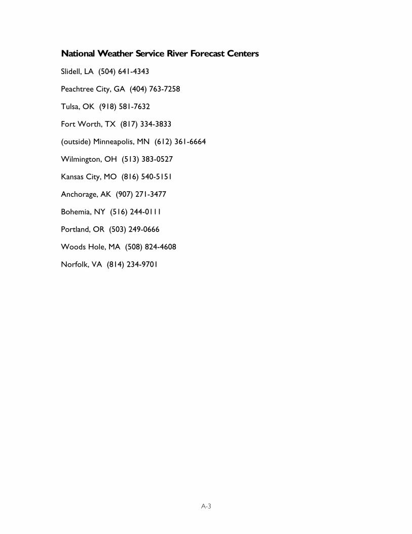
National Weather Service River Forecast Centers

Slidell, LA (504) 641-4343

Peachtree City, GA (404) 763-7258

Tulsa, OK (918) 581-7632

Fort Worth, TX (817) 334-3833

(outside) Minneapolis, MN (612) 361-6664

Wilmington, OH (513) 383-0527

Kansas City, MO (816) 540-5151

Anchorage, AK (907) 271-3477

Bohemia, NY (516) 244-0111

Portland, OR (503) 249-0666

Woods Hole, MA (508) 824-4608

Norfolk, VA (814) 234-9701

A-3

46