phys3001 classical mechanics -...

PHYS3001Classical Mechanics

Robert L. DewarDepartment of Theoretical Physics

Research School of Physical Sciences & EngineeringThe Australian National University

Canberra ACT 0200Australia

[email protected]

Version 1.51

May 20, 2001. c© R.L. Dewar 1998–2001.

Contents

1 Generalized Kinematics 11.1 Introduction . . . . . . . . . . . . . . . . . . . . . . . . . . . . 11.2 Generalized coordinates . . . . . . . . . . . . . . . . . . . . . 21.3 Example: The ideal fluid . . . . . . . . . . . . . . . . . . . . . 51.4 Variational Calculus . . . . . . . . . . . . . . . . . . . . . . . 6

1.4.1 Example: Geodesics . . . . . . . . . . . . . . . . . . . 91.4.2 Trial function method . . . . . . . . . . . . . . . . . . 10

1.5 Constrained variation: Lagrange multipliers . . . . . . . . . . 101.6 Problems . . . . . . . . . . . . . . . . . . . . . . . . . . . . . . 13

1.6.1 Rigid rod . . . . . . . . . . . . . . . . . . . . . . . . . 131.6.2 Ecliptic . . . . . . . . . . . . . . . . . . . . . . . . . . 131.6.3 Curvature of geodesics . . . . . . . . . . . . . . . . . . 13

2 Lagrangian Mechanics 152.1 Introduction . . . . . . . . . . . . . . . . . . . . . . . . . . . . 152.2 Generalized Newton’s 2nd Law . . . . . . . . . . . . . . . . . 16

2.2.1 Generalized force . . . . . . . . . . . . . . . . . . . . . 162.2.2 Generalized equation of motion . . . . . . . . . . . . . 202.2.3 Example: Motion in Cartesian coordinates . . . . . . . 21

2.3 Lagrange’s equations (scalar potential case) . . . . . . . . . . 212.3.1 Hamilton’s Principle . . . . . . . . . . . . . . . . . . . 23

2.4 Lagrangians for some Physical Systems . . . . . . . . . . . . . 242.4.1 Example 1: 1-D motion—the pendulum . . . . . . . . 242.4.2 Example 2: 2-D motion in a central potential . . . . . 252.4.3 Example 3: 2-D motion with time-varying constraint . 262.4.4 Example 4: Atwood’s machine . . . . . . . . . . . . . . 272.4.5 Example 5: Particle in e.m. field . . . . . . . . . . . . 282.4.6 Example 6: Particle in ideal fluid . . . . . . . . . . . . 29

2.5 Averaged Lagrangian . . . . . . . . . . . . . . . . . . . . . . . 302.5.1 Example: Harmonic oscillator . . . . . . . . . . . . . . 31

2.6 Transformations of the Lagrangian . . . . . . . . . . . . . . . 32

iii

iv CONTENTS

2.6.1 Point transformations . . . . . . . . . . . . . . . . . . . 322.6.2 Gauge transformations . . . . . . . . . . . . . . . . . . 34

2.7 Symmetries and Noether’s theorem . . . . . . . . . . . . . . . 352.7.1 Time symmetry . . . . . . . . . . . . . . . . . . . . . . 37

2.8 Problems . . . . . . . . . . . . . . . . . . . . . . . . . . . . . . 372.8.1 Coriolis force and cyclotron motion . . . . . . . . . . . 372.8.2 Anharmonic oscillator . . . . . . . . . . . . . . . . . . 38

3 Hamiltonian Mechanics 413.1 Introduction: Dynamical systems . . . . . . . . . . . . . . . . 413.2 Mechanics as a dynamical system . . . . . . . . . . . . . . . . 41

3.2.1 Lagrangian method . . . . . . . . . . . . . . . . . . . . 413.2.2 Hamiltonian method . . . . . . . . . . . . . . . . . . . 433.2.3 Example 1: Scalar potential . . . . . . . . . . . . . . . 453.2.4 Example 2: Physical pendulum . . . . . . . . . . . . . 473.2.5 Example 3: Motion in e.m. potentials . . . . . . . . . . 483.2.6 Example 4: The generalized N -body system . . . . . . 48

3.3 Time-Dependent and Autonomous Hamiltonian systems . . . 503.4 Hamilton’s Principle in phase space . . . . . . . . . . . . . . . 503.5 Problems . . . . . . . . . . . . . . . . . . . . . . . . . . . . . . 53

3.5.1 Constraints and moving coordinates . . . . . . . . . . . 533.5.2 Anharmonic oscillator phase space . . . . . . . . . . . 533.5.3 2-D motion in a magnetic field . . . . . . . . . . . . . . 53

4 Canonical transformations 554.1 Introduction . . . . . . . . . . . . . . . . . . . . . . . . . . . . 554.2 Generating functions . . . . . . . . . . . . . . . . . . . . . . . 56

4.2.1 Example 1: Adiabatic Oscillator . . . . . . . . . . . . . 604.2.2 Example 2: Point transformations . . . . . . . . . . . . 62

4.3 Infinitesimal canonical transformations . . . . . . . . . . . . . 634.3.1 Time evolution . . . . . . . . . . . . . . . . . . . . . . 64

4.4 Poisson brackets . . . . . . . . . . . . . . . . . . . . . . . . . . 654.4.1 Symmetries and integrals of motion . . . . . . . . . . . 664.4.2 Perturbation theory . . . . . . . . . . . . . . . . . . . . 66

4.5 Action-Angle Variables . . . . . . . . . . . . . . . . . . . . . . 674.6 Properties of canonical transformations . . . . . . . . . . . . . 69

4.6.1 Preservation of phase-space volume . . . . . . . . . . . 694.6.2 Transformation of Poisson brackets . . . . . . . . . . . 74

4.7 Problems . . . . . . . . . . . . . . . . . . . . . . . . . . . . . . 744.7.1 Coriolis yet again . . . . . . . . . . . . . . . . . . . . . 744.7.2 Difference approximations . . . . . . . . . . . . . . . . 75

CONTENTS v

5 Answers to Problems 775.1 Chapter 1 Problems . . . . . . . . . . . . . . . . . . . . . . . . 775.2 Chapter 2 Problems . . . . . . . . . . . . . . . . . . . . . . . . 805.3 Chapter 3 Problems . . . . . . . . . . . . . . . . . . . . . . . . 865.4 Chapter 4 Problems . . . . . . . . . . . . . . . . . . . . . . . . 93

6 References and Index 99

vi CONTENTS

Chapter 1

Generalized coordinates andvariational principles

1.1 Introduction

In elementary physics courses you were introduced to the basic ideas of New-tonian mechanics via concrete examples, such as motion of a particle in agravitational potential, the simple harmonic oscillator etc. In this course wewill develop a more abstract viewpoint in which one thinks of the dynamics ofa system described by an arbitrary number of generalized coordinates, but inwhich the dynamics can be nonetheless encapsulated in a single scalar func-tion: the Lagrangian, named after the French mathematician Joseph LouisLagrange (1736–1813), or the Hamiltonian, named after the Irish mathe-matician Sir William Rowan Hamilton (1805–1865).

This abstract viewpoint is enormously powerful and underpins quantummechanics and modern nonlinear dynamics. It may or may not be more ef-ficient than elementary approaches for solving simple problems, but in orderto feel comfortable with the formalism it is very instructive to do some ele-mentary problems using abstract methods. Thus we will be revisiting suchexamples as the harmonic oscillator and the pendulum, but when examplesare set in this course please remember that you are expected to use the ap-proaches covered in the course rather than fall back on the methods youlearnt in First Year.

In the following notes the convention will be used of italicizing the first useor definition of a concept. The index can be used to locate these definitionsand the subsequent occurrences of these words.

The present chapter is essentially geometric. It is concerned with the de-scription of possible motions of general systems rather than how to calculate

1

2CHAPTER 1. GENERALIZED COORDINATES AND VARIATIONAL PRINCIPLES

physical motions from knowledge of forces. Thus we call the topic generalizedkinematics .

1.2 Generalized coordinates

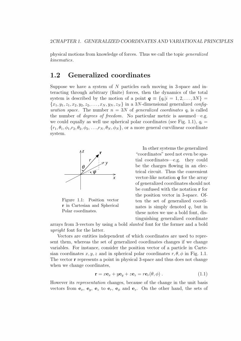
Suppose we have a system of N particles each moving in 3-space and in-teracting through arbitrary (finite) forces, then the dynamics of the totalsystem is described by the motion of a point q ≡ qi|i = 1, 2, . . . , 3N =x1, y1, z1, x2, y2, z2, . . . , xN , yN , zN in a 3N -dimensional generalized config-uration space. The number n = 3N of generalized coordinates qi is calledthe number of degrees of freedom. No particular metric is assumed—e.g.we could equally as well use spherical polar coordinates (see Fig. 1.1), qi =r1, θ1, φ1,r2, θ2, φ2, . . .,rN , θN , φN, or a more general curvilinear coordinatesystem.

In other systems the generalized

x

θr

φ

y

z r

Figure 1.1: Position vectorr in Cartesian and SphericalPolar coordinates.

“coordinates” need not even be spa-tial coordinates—e.g. they couldbe the charges flowing in an elec-trical circuit. Thus the convenientvector-like notation q for the arrayof generalized coordinates should notbe confused with the notation r forthe position vector in 3-space. Of-ten the set of generalized coordi-nates is simply denoted q, but inthese notes we use a bold font, dis-tinguishing generalized coordinate

arrays from 3-vectors by using a bold slanted font for the former and a boldupright font for the latter.

Vectors are entities independent of which coordinates are used to repre-sent them, whereas the set of generalized coordinates changes if we changevariables. For instance, consider the position vector of a particle in Carte-sian coordinates x, y, z and in spherical polar coordinates r, θ, φ in Fig. 1.1.The vector r represents a point in physical 3-space and thus does not changewhen we change coordinates,

r = xex + yey + zez = rer(θ, φ) . (1.1)

However its representation changes, because of the change in the unit basisvectors from ex, ey, ez to er, eφ and ez. On the other hand, the sets of

1.2. GENERALIZED COORDINATES 3

generalized coordinates rC ≡ x, y, z and rsph ≡ r, φ, z are distinct enti-ties: they are points in two different (though related) configuration spacesdescribing the particle.

q1

q2

q3 ... q

n

q(t)q(t1)

q(t2)

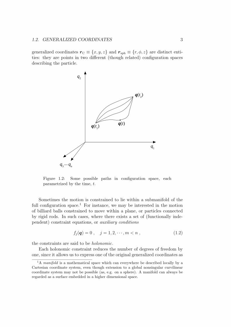
Figure 1.2: Some possible paths in configuration space, eachparametrized by the time, t.

Sometimes the motion is constrained to lie within a submanifold of thefull configuration space.1 For instance, we may be interested in the motionof billiard balls constrained to move within a plane, or particles connectedby rigid rods. In such cases, where there exists a set of (functionally inde-pendent) constraint equations, or auxiliary conditions

fj(q) = 0 , j = 1, 2, · · · ,m < n , (1.2)

the constraints are said to be holonomic.Each holonomic constraint reduces the number of degrees of freedom by

one, since it allows us to express one of the original generalized coordinates as

1A manifold is a mathematical space which can everywhere be described locally by aCartesian coordinate system, even though extension to a global nonsingular curvilinearcoordinate system may not be possible (as, e.g. on a sphere). A manifold can always beregarded as a surface embedded in a higher dimensional space.


a function of the others and delete it from the set. For instance, for a particleconstrained to move in a horizontal plane (an idealized billiard table), thevertical position z = const is a trivial function of the horizontal coordinatesx and y and the configuration space becomes two dimensional, q = x, y.

Consider the set of all conceivable paths through configuration space (seeFig. 1.2). Each one may be parametrized by the time, t: q = q(t). Bydifferentiating eq. (1.2) with respect to time, we find a set of constraints onthe generalized velocities, qi ≡ dqi/ dt, which we write in differential notationas

n∑i=1

∂fj(q)

∂qidqi ≡

∂fj(q)

∂q· dq = 0 , (1.3)

where ∂f/∂q ≡ ∂f/∂q1, . . . , ∂f/∂qn and we use the shorthand dot-productnotation

a·∂f∂b

≡n∑

i=1

ai∂f

∂bi, (1.4)

where ai and bi are arbitrary configuration space variables.The condition for functional independence of the m constraints is that

there be m nontrivial solutions of eq. (1.3), i.e. that the rank of the matrix∂fj(q)/∂qi be its maximal possible value, m.

Note that not all such differential constraints lead to holonomic con-straints. If we are given constraints as a general set of differential forms

n∑i=1

ω(j)i (q) dqi = 0 , (1.5)

then we may or may not be able to integrate the constraint equations to theform eq. (1.2). When we can, the forms are said to be complete differentials.When we cannot, the constraints are said to be nonholonomic.

The latter case, where we cannot reduce the number of degrees of freedomby the number of constraints, will not be considered explicitly in these notes.Furthermore, we shall normally assume that any holonomic constraints havebeen used to reduce qi|i = 1, . . . , n to a minimal, unconstrained set. How-ever, we present in Sec. 1.5 an elegant alternative that may be used whenthis reduction is not convenient, or is impossible due to the existence ofnonholonomic constraints.

There are situations where there is an infinite number of generalizedcoordinates. For instance, consider a scalar field (such as the instaneousamplitude of a wave), ψ(r, t). Here ψ is a generalized coordinate of thesystem and the position vector r replaces the index i. Since r is a continuousvariable it ranges over an infinite number of values.

1.3. EXAMPLE: THE IDEAL FLUID 5

r0

x(r0,t)

Figure 1.3: A fluid element advected from point r = r0 at time t = 0to r = x(r0, t) at time t.

1.3 Example: The ideal fluid

As an example of a system with both an infinite number of degrees of freedomand holonomic constraints, consider a fluid with density field ρ(r, t), pressurefield p(r, t) and velocity field v(r, t).

Here we are using the Eulerian description, where the fluid quantities ρ,p and v are indexed by the actual position, r, at which they take on theirphysical values at each point in time.

However, we can also index these fields by the initial position, r0, ofthe fluid particle passing through the point r = x(r0, t) at time t (seeFig. 1.3). This is known as the Lagrangian description. (cf. the Schrodingerand Heisenberg pictures in quantum mechanics.) We shall denote fields inthe Lagrangian description by use of a subscript L: ρL(r0, t), pL(r0, t) andvL(r0, t) = ∂tx(r0, t).

The field x(r0, t) may be regarded as an infinite set of generalized coor-dinates, the specification of which gives the state of the fluid at time t. TheJacobian J(r0, t) of the change of coordinates r = x(r0, t) is defined by

J ≡ ∂x

∂x0

· ∂x∂y0

× ∂x

∂z0

=

∣∣∣∣∣∣∣∂x∂x0

∂y∂x0

∂z∂x0

∂x∂y0

∂y∂y0

∂z∂y0

∂x∂z0

∂y∂z0

∂z∂z0

∣∣∣∣∣∣∣ , (1.6)

where x0, y0 and z0 are Cartesian components of r0 and x, y and z are thecorresponding components of x(r0, t). This gives the change of volume ofa fluid element with initial volume dV0 and final volume (at time t) dVthrough

dV = J(r0, t) dV0 . (1.7)

To see this, consider dV0 = dx0 dy0 dz0 to be an infinitesimal rectangularbox, as indicated in Fig. 1.3, with sides of length dx0, dy0, dz0. This fluid


element is transformed by the effect of compression and shear to an infinites-imal parallelipiped with sides given by dlx ≡ dx0∂x/∂x0, dly ≡ dy0∂x/∂y0,dlz ≡ dz0∂x/∂z0. The volume of such a parallepiped is dlx· dly× dlz =J dx0 dy0 dz0 2.

Are the fields ρ(r0, t) and p(r0, t) additional generalized coordinates whichneed to be specified at each point in time? In an ideal fluid (i.e. one withno dissipation, also called an Euler fluid) the answer is no, because massconservation, ρ dV = ρ0 dV0, allows us to write

ρL(r0, t) = ρ0(r0)/J(r0, t) , (1.8)

while the ideal equation of state p( dV )γ = p0( dV0)γ, where γ is the ratio of

specific heats, givespL(r0, t) = p0(r0)/J

γ(r0, t) , (1.9)

where ρ0 and p0 are the initial density and pressure fields, respectively. Theseare, by definition, fixed in time, so the only time dependence occurs throughthe Jacobian J , which we showed in eq. (1.6) to be completely determinedby the Lagrangian displacement field x(r0, t). Thus eqs. (1.8) and (1.9) haveallowed us to reduce the number of generalized coordinate fields from 5 to3 (the three components of x)—mass conservation and the equation of statehave acted as holonomic constraints.

Note: Mass conservation is valid even for nonideal fluids (provided theyare not reacting and thus changing from one state to another). However,in a fluid with finite dissipation, heat will be generated by the motion andentropy will be increased in each fluid element, thus invalidating the useof the adiabatic equation of state. Further, the entropy increase dependson the complete path of the fluid through its state space, not just on itsinstantaneous state. Thus the pressure cannot be holonomically constrainedin a nonideal fluid.

Remark 1.1 A useful model for a hot plasma is the magnetohydrodynamic(MHD) fluid—an ideal fluid with the additional property of being a perfectelectrical conductor. This leads to the magnetic field B(r, t) being “frozen in”to the plasma, so that BL also obeys a holonomic constraint in the Lagrangianrepresentation, but as it is a vector constraint it is a little too complicated togive here.

1.4 Variational Calculus

Consider an objective functional I[q], defined on the space of all differentiablepaths between two points in configuration space, q(t1) and q(t2), as depicted

1.4. VARIATIONAL CALCULUS 7

in Fig. 1.2

I[q] ≡∫ t2

t1

dt f(q(t), q(t), t) . (1.10)

(As we shall wish to integrate by parts later, we in fact assume the paths tobe slightly smoother than simply differentiable, so that q is also defined.)

We suppose our task is to find a path that makes I a maximum or min-imum (or at least stationary) with respect to neighbouring paths. Thus wevary the path by an amount δq(t): q(t) 7→ q(t) + δq(t). Then the firstvariation, δI, is defined to be the change in I as estimated by linearizing inδq:

δI[q] ≡∫ t2

t1

dt

[δq(t)·∂f

∂q+ δq(t)·∂f

∂q

]. (1.11)

Our first task is to evaluate eq. (1.11) in terms of δq(t). The crucial stephere is the lemma “delta and dot commute”. That is

δq ≡ dδq

dt. (1.12)

To prove this, simply go back to definitions: δq ≡ d(q + δq)/ dt− dq/ dt =dδq/ dt 2.

We can now integrate by parts to put δI in the form

δI[q] =

[δq·∂f

∂q

]t2

t1

+

∫ t2

t1

dt δq(t)·δfδq

. (1.13)

This consists of an endpoint contribution and an integral of the variationalderivative δf/δq, defined by

δf

δq≡ ∂f

∂q− d

dt

∂f

∂q. (1.14)

Remark 1.2 The right-hand side of eq. (1.14) is also sometimes called thefunctional derivative or Frechet derivative of I[q]. When using this termi-nology the notation δI/δq is used instead of δf/δq so that we can writeeq. (1.13), for variations δqi which vanish in the neighbourhood of the end-points, as

δI[q] ≡∫ t2

t1

dtn∑

i=1

δqi(t)δI

δqi(t) ,

≡(δq,

δI

δq

), (1.15)


which may be taken as the most general defining equation for δI/δq. Theinner product notation (·, ·) used above is a kind of infinite-dimensional dotproduct where we not only sum over the index i, but integrate over the “index”t. If we recall that the change in the value of a field defined on 3-space, e.g.ϕ(r), due to an arbitrary infinitesimal change δr is δϕ = δr·∇ϕ, which maybe regarded as the definition of the gradient ∇ϕ, we see that the functionalderivative δI/δq may be thought of, by analogy, as an infinite-dimensionalgradient defined on the function space of paths.

A typical variational problem is to make I extremal or stationary underarbitrary variations δq(t) holding the endpoints fixed. That is, we require

δI = 0 ∀ functions δq(t) such that δq(t1) = δq(t2) = 0 . (1.16)

Note that this condition does not necessarily require I to be a minimumor maximum—it can be a kind of saddle point in function space, with someascending and some descending “directions”. To determine the nature ofa stationary point we would need to expand I to second order in δq—thesecond variation.

In the class of variations in eq.

t + ε

qi

t − ε

Figure 1.4: A time-localizedvariation in generalized coor-dinate qi with support in therange t− ε to t+ ε.

(1.16), the endpoint contribution ineq. (1.13) vanishes, leaving onlythe contribution of the integral overt. Since δq(t) is arbitrary, we can,in particular, consider functions witharbitrarily localized support in t, asindicated in Fig. 1.4. (The supportof a function is just the range overwhich it is nonzero.) As ε → 0,δf/δq(t) becomes essentially con-stant over the support of q in eq. (1.13)and we can move it outside the in-tegral. Clearly then, I can only be

stationary for all such variations if and only if the variational derivative van-ishes for each value of t and each index i

δf

δq= 0 . (1.17)

These n equations are known as the Euler–Lagrange equations . Some-times we encounter variational problems where we wish to extremize I under

1.4. VARIATIONAL CALCULUS 9

variations of the endpoints as well, δq(t1) 6= δq(t2) 6= 0. In such cases wesee from eq. (1.13) that, in addition to eq. (1.17), stationarity implies thenatural boundary conditions

∂f

∂q= 0 (1.18)

at t1 and t2.

1.4.1 Example: Geodesics

In the above development we have used the symbol t to denote the indepen-dent variable because, in applications in dynamics, paths in configurationspace are naturally parametrized by the time. However, in purely geometricapplications t is simply an arbitrary label for the position along a path, andwe shall in this section denote it by τ to avoid confusion.

The distance along a path is given by integrating the lengths dl of in-finitesimal line elements, given a metric tensor gi,j such that

( dl)2 =n∑

i,j=1

dqi gi,j dqj . (1.19)

In terms of our parameter τ , we thus have the length l as a functional of theform discussed above

l =

∫ τ2

τ1

dτ

[n∑

i,j=1

qigi,j(q, τ)qj

]1/2

. (1.20)

A geodesic is a curve between two points whose length (calculated usingthe given metric) is stationary against infinitesimal variations about thatpath. Thus the task of finding geodesics fits within the class of variationalproblems we have discussed, and we can use the Euler–Lagrange equationsto find them. Perhaps the best known result on geodesics is the fact that theshortest path between two points in a Euclidean space (one where gi,j = 0for i 6= j and gi,j = 1 for i = j) is a straight line. Another well-known resultis that the shortest path between two points on the surface of a sphere is agreat circle (see Problem 1.6.3 for a general theorem on geodesics on a curvedsurface).

Geodesics are not necessarily purely geometrical objects, but can havephysical interpretations. For instance, suppose we want to find the shape ofan elastic string stretched over a slippery surface. The string will adjust itsshape to minimize its elastic energy. Since the elastic potential energy is a


monotonically increasing function of the length of the string, the string willsettle onto a geodesic on the surface.

Geodesics also play an important role in General Relativity, because theworld line of a photon is a geodesic in 4-dimensional space time, with themetric tensor obeying Einstein’s equations. If the metric is sufficiently dis-torted, it can happen that there is not one, but several geodesics betweentwo points, a fact which explains the phenomenon of gravitational lensing(multiple images of a distant galaxy behind a closer massive object).

1.4.2 Trial function method

One advantage of the variational formulation of a problem is that we canuse trial function methods to find approximate solutions. That is, we canmake a clever guess, q(t) = qK(t, a1, a2, . . . , aK) as to the general form ofthe solution, using some specific function qK (the trial function) involving afinite number of parameters ak, k = 1, . . . , K. Then we evaluate the integralin eq. (1.11) (analytically or numerically) and seek a stationary point ofthe resulting function I(a1, a2, . . . , aK) in the K-dimensional space of theparameters ak. Varying the ak the variation in I is

δI =K∑

k=1

∂I

∂ak

δak . (1.21)

The condition for a stationary point is thus

∂I

∂ak

= 0, k = 1, . . . , K , (1.22)

that is, that the K-dimensional gradient of I vanish.Since the true solution makes the objective functional I stationary with

respect to small variations, if our guessed trial function solution is close tothe true solution the error in I will be small. (Of course, because qK maynot be a reasonable guess for the solution in all ranges of the parameters,there may be spurious stationary points that must be rejected because theycannot possibly be close to a true solution—see the answer to Problem 2.8.2in Sec. 5.2.)

1.5 Constrained variation: Lagrange multi-

pliers

As mentioned in Sec. 1.2 we normally assume that the holonomic constraintshave been used to reduce the dimensionality of the configuration space so

1.5. CONSTRAINED VARIATION: LAGRANGE MULTIPLIERS 11

that all variations are allowed. However, it may not be possible to do ananalytic elimination explicitly. Or it may be that some variables appear ina symmetric fashion, making it inelegant to eliminate one in favour of theothers.

Thus, even in the holonomic case, it is worth seeking a method of han-dling constrained variations : when there are one or more differential auxiliaryconditions of the form δf (j) = 0. In the nonholonomic case it is mandatoryto consider such variations because the auxiliary conditions cannot be inte-grated.

We denote the dimension of the configuration space by n. Followingeq. (1.5) we suppose there are m < n auxiliary conditions of the form

δf (j) ≡ ω(j)(q, t)·δq = 0 . (1.23)

The vectors ω(j), j = 1, . . . ,m may be assumed linearly independent (elsesome of the auxiliary conditions would be redundant) and thus span an m-dimensional subspace, Vm(t), of the full n-dimensional linear vector spaceVn occupied by the unconstrained variations. Thus the equations eq. (1.23)constrain the variations δq to lie within an (n − m)-dimensional subspace,Vn−m(q, t), complementary to Vn.

The variational problem we seek to solve is to find the conditions (thegeneralizations of the Euler–Lagrange equations) under which the objectivefunctional I[q] is stationary with respect to all variations δq in Vm(q, t).Apart from this restriction on the variations, the problem is the same as thatdescribed by eq. (1.16). The generalization of eq. (1.17) is

δf

δq·δq = 0 ∀ δq ∈ Vn−m(q, t) . (1.24)

If there are no constraints, so that m = 0, then δf/δq is orthogonal toall vectors in Vn and the only solution is that δf/δq ≡ 0. Thus eq. (1.24)and eq. (1.17) are equivalent in this case. However, if m < n, then δf/δqcan have a nonvanishing component in the subspace Vm and eq. (1.17) is nolonger valid.

An elegant solution to the problem of generalizing eq. (1.17) was found byLagrange. Expressed in our linear vector space language, his idea was thateq. (1.24) can be regarded as the statement that the projection, (δf/δq)n−m,of δf/δq into Vn−m(q, t) is required to vanish.

However, we can write (δf/δq)n−m as δf/δq−(δf/δq)m, where (δf/δq)m

is the projection of δf/δq into Vm. Now observe that we can write any vectorin Vm as a linear superposition of the ω(j) since they form a basis spanning


this space. Thus we write (δf/δq)m = −∑λjω

(j), or, equivalently,(δf

δq

)m

+m∑

j=1

λjω(j) = 0 , (1.25)

where the λj(q, t) coefficients, as yet to be determined, are known as theLagrange multipliers . They can be determined by dotting eq. (1.25) with eachof the m basis vectors ω(j), thus providing m equations for the m unknowns.Alternatively, we can express this variationally as[(

δf

δq

)m

+m∑

j=1

λjω(j)

]·δq = 0 ∀ δq ∈ Vm(q, t) . (1.26)

Since −∑λjω

(j) is the projection into Vm of δf/δq, the projection intothe complementary subspace Vn−m is found by subtracting (−

∑λjω

(j)) fromδf/δq. That is, (

δf

δq

)n−m

=δf

δq+

m∑j=1

λjω(j)

= 0 , (1.27)

where the Vn−m component of the second equality follows by eq. (1.24) andthe Vn component from eq. (1.25). Thus we have n generalized Euler–Lagrange equations, but they incorporate the m equations for the, so fararbitrary, λ(j) implicit in eq. (1.25). Thus we really only gain (n−m) equa-tions from the variational principle, which is at it should be because we alsoget m kinematic equations from the constraint conditions—if we got morefrom the variational principle the problem would be overdetermined.

The variational formulation of the second equality in eq. (1.27) is[δf

δq+

m∑j=1

λjω(j)

]·δq = 0 ∀ δq ∈ Vn(q, t) . (1.28)

That is, by using the Lagrange multipliers we have turned the constrainedvariational problem into an unconstrained one.

In the holonomic case, when the auxiliary conditions are of the form ineq. (1.2), we may derive eq. (1.28) by unconstrained variation of the modifiedobjective functional

I∗[q] ≡∫ t2

t1

dt (f +m∑

j=1

λjfj) . (1.29)

The auxiliary conditions also follow from this functional if we require that itbe stationary under variation of the λj.

1.6. PROBLEMS 13

1.6 Problems

1.6.1 Rigid rod

Two particles are connected by a rigid rod so they are constrained to move afixed distance apart. Write down a constraint equation of the form eq. (1.2)and find suitable generalized coordinates for the system incorporating thisholonomic constraint.

1.6.2 Ecliptic

Suppose we know that the angular momentum vectors rk×mkrk of a systemof particles are all nonzero and parallel to the z-axis in a particular Cartesiancoordinate system. Write down the differential constraints implied by thisfact, and show that they lead to a set of holonomic constraints. Hence writedown suitable generalized coordinates for the system.

1.6.3 Curvature of geodesics

Show that any geodesic r = x(τ) on a two-dimensional manifold S : r =X(θ, ζ) embedded in ordinary Euclidean 3-space, where θ and ζ are arbi-trary curvilinear coordinates on S, is such that the curvature vector κ(τ) iseverywhere normal to S (or zero).

The curvature vector is defined by κ ≡ de‖/ dl, where e‖(τ) ≡ dx/ dl isthe unit tangent vector at each point along the path r = x(τ).

Hint: First find f(θ, ζ, θ, ζ) = l, the integrand of the length functional,l =

∫f dτ (which involves finding the metric tensor in θ, ζ space in terms of

∂X/∂θ and ∂X/∂ζ). Then show that, for any path on S,

∂f

∂θ= e‖·

∂X

∂θ

(and similarly for the ζ derivative) and

∂f

∂θ= e‖·

d

dτ

∂X

∂θ,

and again similarly for the ζ derivative.

Chapter 2

Lagrangian Mechanics

2.1 Introduction

The previous chapter dealt with generalized kinematics—the description ofgiven motions in time and space. In this chapter we deal with one formula-tion (due to Lagrange) of generalized dynamics—the derivation of differentialequations (equations of motion) for the time evolution of the generalized co-ordinates. Given appropriate initial conditions, these (in general, nonlinear)equations of motion specify the motion uniquely. Thus, in a sense, the mostimportant task of the physicist is over when the equations of motion havebeen derived—the rest is just mathematics or numerical analysis (importantthough these are). The goal of generalized dynamics is to find universal formsof the equations of motion.

From elementary mechanics we are all familiar with Newton’s SecondLaw, F = ma for a particle of mass m subjected to a force F and undergoingan acceleration a ≡ r. If we know the Cartesian components Fi(r, r, t),i = 1, 2, 3, of the force in terms of the Cartesian coordinates x1 = x, x2 = y,x3 = z and their first time derivatives then the equations of motion are theset of three second-order differential equations mxi − Fi = 0.

To give a physical framework for developing our generalized dynamicalformalism we consider a set of N Newtonian point masses, which may be con-nected by holonomic constraints so the number n of generalized coordinatesmay be less than 3N . Indeed, in the case of a rigid body N is essentiallyinfinite, but the number of generalized coordinates is finite. For example,the generalized coordinates for a rigid body could be the three Cartesiancoordinates of the centre of mass and three angles to specify its orientation(known as the Euler angles), so n = 6 for a rigid body allowed to move freelyin space.

15

16 CHAPTER 2. LAGRANGIAN MECHANICS

Whether the point masses are real particles like electrons, composite par-ticles like nuclei or atoms, or mathematical idealizations like the infinitesimalvolume elements in a continuum description, we shall refer to them generi-cally as “particles”.

Having found a very general form of the equations of motion (Lagrange’sequations), we then find a variational principle (Hamilton’s Principle) thatgives these equations as its Euler–Lagrange equations in the case of no fric-tional dissipation. This variational principle forms a basis for generalizingeven beyond Newtonian mechanics (e.g. to dynamics in Special Relativity).

2.2 Generalized Newton’s 2nd Law

2.2.1 Generalized force

Let the (constrained) position of each of the N particles making up the sys-tem be given as a function of the n generalized coordinates q by rk = xk(q, t),k = 1, . . . , N . If there are holonomic constraints acting on the particles, thenumber of generalized coordinates satisfies the inequality n ≤ 3N . Thus, thesystem may be divided into two subsystems—an “exterior” subsystem de-scribed by the n generalized coordinates and an “interior” constraint subsys-tem whose (3N−n) coordinates are rigidly related to the q by the geometricconstraints.

In a naive Newtonian approach we would have to specify the forces act-ing on each particle (taking into account Newton’s Third Law, “action andreaction are equal and opposite”), derive the 3N equations of motion foreach particle and then eliminate all the interior subsystem coordinates tofind the equations of motion of the generalized coordinates only. This isclearly very inefficient, and we already know from elementary physics thatit is unnecessary—we do not really need an infinite number of equations todescribe the motion of a rigid body. What we seek is a formulation in whichonly the generalized coordinates, and generalized forces conjugate to them,appear explicitly. All the interior coordinates and the forces required to main-tain their constrained relationships to each other (the “forces of constraint”)should be implicit only.

To achieve this it turns out to be fruitful to adopt the viewpoint thatthe total mechanical energy (or, rather, its change due to the performance ofexternal work, W , on the system) is the primitive concept, rather than thevector quantity force. The basic reason is that the energy, a scalar quantity,needs only specification of the coordinates for its full description, whereasthe representation of the force, a vector, depends also on defining a basis

2.2. GENERALIZED NEWTON’S 2ND LAW 17

set on which to resolve it. The choice of basis set is not obvious when weare using generalized coordinates. [Historically, force came to be understoodearlier, but energy also has a long history, see e.g. Ernst Mach “The Scienceof Mechanics” (Open Court Publishing, La Salle, Illinois, 1960) pp. 309–312,QA802.M14 Hancock. With the development of Lagrangian and Hamiltonianmethods, and thermodynamics, energy-based approaches can now be said tobe dominant in physics.]

To illustrate the relation between force and work, first consider justone particle. Recall that the work δW done on the particle by a forceF as the particle suffers an infinesimal displacement δr is δW = F·δr ≡Fxδx+Fyδy+Fzδz. A single displacement δr does not give enough informa-tion to determine the three components of F, but if we imagine the thoughtexperiment of displacing the particle in the three independent directions,δr = δx ex, δy ey and δz ez, determining the work, δWx, δWy, δWz, done ineach case, then we will have enough equations to deduce the three compo-nents of the force vector, Fx = δWx/δx, Fy = δWy/δy, Fz = δWz/δz. [IfδW can be integrated to give a function W (r) (which is not always possi-ble), then we may use standard partial derivative notation: Fx = ∂W/∂x,Fy = ∂W/∂y, Fz = ∂W/∂z.]

The displacements δx ex, δy ey and δz ez are historically called virtualdisplacements . They are really simply the same displacements as used inthe mathematical definition of partial derivatives. Note that the virtualdisplacements are done at a fixed instant in time as if by some “invisiblehands”, which perform the work δW : this is a thought experiment—thedisplacements are fictitious, not dynamical.

Suppose we now transform from the Cartesian coordinates x, y, z to anarbitrary curvilinear coordinate system q1, q2, q3 (the superscript notationbeing conventional in tensor calculus). Then an arbitrary virtual displace-ment is given by δr =

∑i δq

i ei, where the basis vectors ei are in general notorthonormal. The corresponding “virtual work” is given by δW =

∑i δq

i Fi,where Fi ≡ ei·F. As in the Cartesian case, this can be used to determine thegeneralized forces Fi by determining the virtual work done in three indepen-dent virtual displacements.

In tensor calculus the set Fi is known as the covariant representation ofF, and is in general distinct from an alternative resolution, the contravariantrepresentation F i. (You will meet this terminology again in relativitytheory.) The energy approach shows that the covariant, rather than thecontravariant, components of the force form the natural generalized forcesconjugate to the generalized coordinates qi.

Turning now to the N -particle system as a whole, the example abovesuggests we define the set of n generalized forces, Qi, conjugate to each


of the n degrees of freedom qi, to be such that the virtual work done on thesystem in displacing it by an arbitrary infinitesimal amount δq at fixed timet is given by

δW ≡n∑

i=1

Qiδqi ∀ δq . (2.1)

We now calculate the virtual work in terms of the displacements of the Nparticles assumed to make up the system and the forces Fk acting on them.The virtual work is

δW =N∑

k=1

Fk·δrk

=n∑

i=1

δqi

(N∑

k=1

Fk·∂xk

∂qi

). (2.2)

Comparing eq. (2.1) and eq. (2.2), and noting that they hold for any δq, wecan in particular take all but one of the δqi to be zero to pick out the ithcomponent, giving the generalized force as

Qi =N∑

k=1

Fk·∂xk

∂qi. (2.3)

When there are holonomic constraints on the system we decompose theforces acting on the particles into what we shall call explicit forces and forcesof constraint . (The latter terminology is standard, but the usage “explicitforces” seems new—often they are called “applied forces”, but this is confus-ing because they need not originate externally to the system, but also frominteractions between the particles.)

By forces of constraint, Fcstk , we mean those imposed on the particles

by the rigid rods, joints, sliding planes etc. that make up the holonomicconstraints on the system. These forces simply adjust themselves to whatevervalues are required to maintain the geometric constraint equations and canbe regarded as “private” forces that, for most purposes, we do not need toknow1. Furthermore, we may not be able to tell what these forces need tobe until we have solved the equations of motion, so they cannot be assumedknown a priori.

The explicit force on each particle, Fxplk , is the vector sum of any externally

imposed forces, such as those due to an external gravitational or electric field,plus any interaction forces between particles such as those due to elastic

1Of course, in practical engineering design contexts one should at some stage check thatthe constraint mechanism is capable of supplying the required force without deforming orbreaking!

2.2. GENERALIZED NEWTON’S 2ND LAW 19

springs coupling point masses, or to electrostatic attractions between chargedparticles. If there is friction acting on the particle, including that due toconstraint mechanisms, then that must be included in Fxpl

k as well. Theseare the “public” forces that determine the dynamical evolution of the degreesof freedom of the system and are determined by the configuration q of thesystem at each instant of time, and perhaps by the generalized velocity q inthe case of velocity-dependent forces such as those due to friction and thoseacting on a charged particle moving in a magnetic field.

Figure 2.1 shows a simple system withN

mg

F

α

Figure 2.1: A body onan inclined plane as de-scribed in the text.

a holonomic constraint—a particle slid-ing on a plane inclined at angle α. It issubject to the force of gravity, mg, thenormal force N, and a friction force F inthe directions shown. The force of con-straint is N. It does no work because itis orthogonal to the direction of motion,and its magnitude is that required to nullout the normal component of the gravita-tional force, |N| = mg cosα, so as to giveno acceleration in the normal direction and thus maintain the constraint.

We now make the crucial observation that, because the constraints areassumed to be provided by rigid, undeformable mechanisms, no work canbe done on the interior constraint subsystem by the virtual displacements.That is, no (net) virtual work is done against the nonfriction forces imposedby the particles on the constraint mechanisms in performing the variationsδq. By Newton’s Third Law, the nonfriction forces acting on the constraintmechanisms are equal and opposite to the forces of constraint, Fcst

k . Thusthe sum over Fcst

k ·δxk vanishes and we can replace the total force Fk withFxpl

k in eqs. (2.2) and (2.3). Note: If there are friction forces associatedwith the constraints there is work done against these, but this fact does notnegate the above argument because we have included the friction forces inthe explicit forces—any work done against friction forces goes into heat whichis dissipated into the external world, not into mechanical energy within theconstraint subsystem.

That is,

Qi =N∑

k=1

Fxplk ·∂xk

∂qi. (2.4)

For the purpose of calculating the generalized forces, this is a much morepractical expression than eq. (2.3) because the Fxpl

k are known in terms of


the instantaneous positions and velocities. Thus Qi = Qi(q, q, t).

2.2.2 Generalized equation of motion

We now suppose that eq. (2.4) has been used to determine the Q as functionsof the q (and possible q and t if we have velocity-dependent forces and time-dependent constraints, respectively). Then we rewrite eq. (2.3) in the form

N∑k=1

Fk·∂xk

∂qi= Qi(q, q, t) . (2.5)

To derive an equation of motion we use Newton’s second law to replaceFk on the left-hand side of eq. (2.5) with mkrk,

N∑k=1

mkrk·∂xk

∂qi

≡N∑

k=1

mk

[d

dt

(rk·

∂xk

∂qi

)− rk·

d

dt

∂xk

∂qi

]= Qi . (2.6)

We now differentiate rk = xk(q(t), t) with respect to t to find the functionvk such that rk = vk(q, q, t):

rk =∂xk

∂t+

n∑j=1

qj∂xk

∂qj≡ vk(q, q, t) . (2.7)

Differentiating vk wrt qi (treating q and q as independent variables in partialderivatives) we immediately have the lemma

∂xk

∂qi=∂vk

∂qi. (2.8)

The second lemma about partial derivatives of vk that will be needed is

d

dt

∂xk

∂qi=∂vk

∂qi, (2.9)

which follows because d/ dt can be replaced by ∂/∂t + q·∂/∂q, which com-mutes with ∂/∂qi (cf. the “interchange of delta and dot” lemma in Sec. 1.4).

Applying these two lemmas in eq. (2.6) we find

N∑k=1

[d

dt

(mkvk·

∂vk

∂qi

)−mkvk·

∂vk

∂qi

]

=N∑

k=1

[d

dt

∂

∂qi

(12mkv

2k

)− ∂

∂qi

(12mkv

2k

)]= Qi , (2.10)

2.3. LAGRANGE’S EQUATIONS (SCALAR POTENTIAL CASE) 21

In terms of the total kinetic energy of the system, T

T ≡N∑

k=1

12mkv

2k , (2.11)

we write eq. (2.10) compactly as the generalized Newton’s second law

d

dt

∂T

∂qi− ∂T

∂qi= Qi . (2.12)

These n equations are sometimes called Lagrange’s equations of motion, butwe shall reserve this term for a later form [eq. (2.24)] arising when we assumea special (though very general) form for the Qi. They are also sometimescalled (e.g. Scheck p. 83) d’Alembert’s equations, but this may be historicallyinaccurate so is best avoided.

2.2.3 Example: Motion in Cartesian coordinates

Let us check that we can recover Newton’s equations of motion as a specialcase when q = x, y, z. In this case

T = 12m(x2 + y2 + z2) (2.13)

so∂T

∂x=∂T

∂y=∂T

∂z= 0 (2.14)

and∂T

∂x= mx ,

∂T

∂y= my ,

∂T

∂z= mz . (2.15)

Also, from eq. (2.4) we see that Qi ≡ Fi. Substituting in eq. (2.12) weimmediately recover Newton’s 2nd Law in Cartesian form

mx = Fx my = Fy mz = Fy (2.16)

as expected.

2.3 Lagrange’s equations (scalar potential case)

In many problems in physics the forces Fk are derivable from a potential ,V (r1, r2, · · · , rN). For instance, in the classical N -body problem the parti-cles are assumed to interact pairwise via a two-body interaction potential


Vk,l(rk, rl) ≡ Uk,l(|rk − rl|) such that the force on particle k due to particle lis given by

Fk,l = −∇kVk,l

= −(rk − rl)

|rk − rl|U ′

k,l(rk,l) , (2.17)

where the prime on U denotes the derivative with respect to its argument,the interparticle distance rk,l ≡ |rk − rl|. Then the total force on particle kis found by summing the forces on it due to all the other particles

Fk = −∑l 6=k

∇kVk,l

= −∇kV , (2.18)

where the N -body potential V is the sum of all distinct two-body interactions

V ≡N∑

k=1

∑l≤k

Vk,l

= 12

N∑k,l=1

′ Vk,l . (2.19)

In the first line we counted the interactions once and only once: notingthat Vk,l = Vl,k, so that the matrix of interactions is symmetric we havekept only those entries below the diagonal to avoid double counting. In thesecond, more symmetric, form we have summed all the off-diagonal entriesof the matrix but have compensated for the double counting by dividing by2. The exclusion of the diagonal “self-interaction” potentials is indicated byputting a prime on the

∑.

Physical examples of such an N -body system with binary interactionsare:

• An unmagnetized plasma, where Vk,l is the Coulomb interaction

Uk,l(r) =ekel

ε0r, (2.20)

where the ek are the charges on the particles and ε0 is the permittivityof free space. We could also allow for the effect of gravity by addingthe potential

∑k mkgzk to V , where zk is the height of the kth particle

with respect to a horizontal reference plane and mk is its mass.

2.3. LAGRANGE’S EQUATIONS (SCALAR POTENTIAL CASE) 23

• A globular cluster of stars, where Vk,l is the gravitational interaction

Uk,l(r) =Gmkml

r, (2.21)

where G is the gravitational constant.

• A dilute monatomic gas, where Vk,l is the Van der Waal’s interaction.However, if the gas is too dense (or becomes a liquid) we would haveto include 3-body or higher interactions as the wave functions of morethan two atoms could overlap simultaneously.

Even when the system is subjected to external forces, such as gravity,and/or holonomic constraints, we can often still assume that the “explicitforces” are derivable from a potential

Fxplk = −∇kV . (2.22)

Taking into account the constraints, we see that the potential V (r1, r2, · · · , rN)becomes a function, V (q, t), in the reduced configuration space. Then, fromeq. (2.4) we have

Qi = −N∑

k=1

∂xk

∂qi·∇kV

= − ∂

∂qiV (q, t) . (2.23)

Substituting this form for Qi in eq. (2.12) we see that the generalizedNewton’s equations of motion can be encapsulated in the very compact form(Lagrange’s equations of motion)

d

dt

(∂L

∂qi

)− ∂L

∂qi= 0 , (2.24)

where the function L(q, q, t), called the Lagrangian, is defined as

L ≡ T − V . (2.25)

2.3.1 Hamilton’s Principle

Comparing eq. (2.24) with eq. (1.17) we see that Lagrange’s equations ofmotion have exactly the same form as the Euler–Lagrange equations for thevariational principle δS = 0, where the functional S[q], defined by

S ≡∫ t2

t1

dt L(q, q, t) , (2.26)


is known as the action integral . Since the natural boundary conditionseq. (1.18) are not physical, the variational principle is one in which the end-points are to be kept fixed.

We can now state Hamilton’s Principle: Physical paths in configurationspace are those for which the action integral is stationary against all infinites-imal variations that keep the endpoints fixed.

By physical paths we mean those paths, out of all those that are consistentwith the constraints, that actually obey the equations of motion with thegiven Lagrangian.

To go beyond the original Newtonian dynamics with a scalar potentialthat we used to motivate Lagrange’s equations, we can instead take Hamil-ton’s Principle, being such a simple and geometrically appealing result, as amore fundamental and natural starting point for Lagrangian dynamics.

2.4 Lagrangians for some Physical Systems

2.4.1 Example 1: 1-D motion—the pendulum

One of the simplest nonlinear systems is

( 1 −c o s θ ) l

0mg

z

θ l

Figure 2.2: Phys-ical pendulum.

the one-dimensional physical pendulum (so calledto distinguish it from the linearized harmonicoscillator approximation). As depicted in Fig. 2.2,the pendulum consists of a light rigid rod oflength l, making an angle θ with the vertical,swinging from a fixed pivot at one end andwith a bob of mass m attached at the other.

The constraint l = const and the assump-tion of plane motion reduces the system to onedegree of freedom, described by the general-ized coordinate θ. (This system is also calledthe simple pendulum to distinguish it from thespherical pendulum and compound pendula,which have more than one degree of freedom.)The potential energy with respect to the equi-

librium position θ = 0 is V (θ) = mgl(1− cos θ), where g is the accelerationdue to gravity, and the velocity of the bob is vθ = lθ, so that the kineticenergy T = 1

2mv2θ = 1

2ml2θ2. The Lagrangian, T − V , is thus

L(θ, θ) = 12ml

2θ2 −mgl(1− cos θ) . (2.27)

2.4. LAGRANGIANS FOR SOME PHYSICAL SYSTEMS 25

This is also essentially the Lagrangian for a particle moving in a sinusoidalspatial potential, so the physical pendulum provides a paradigm for problemssuch as the motion of an electron in a crystal lattice or of an ion or electronin a plasma wave.

From eq. (2.27) ∂L/∂θ = ml2θ and ∂L/∂θ = −mgl sin θ. Thus, theLagrangian equation of motion is

ml2θ = −mgl sin θ . (2.28)

Expanding the cosine up to quadratic order in θ gives the harmonic os-cillator oscillator approximation (see also Sec. 2.6.2)

L ≈ Llin ≡ 12ml

2θ2 − 12mglθ

2 , (2.29)

for which the equation of motion is, dividing through by ml2, θ + ω20θ = 0,

with ω0 ≡√g/l.

2.4.2 Example 2: 2-D motion in a central potential

Let us work in plane polar coordinates, q = r, θ, such that

x = r cos θ , y = r sin θ , (2.30)

so that

x = r cos θ − rθ sin θ ,

y = r sin θ + rθ cos θ , (2.31)

whence the kinetic energy T ≡ 12(x

2 + y2) is found to be

T = 12m(r2 + r2θ2

). (2.32)

An alternative derivation of eq. (2.32) may be found by resolving v into thecomponents rer and rθeθ, where er is the unit vector in the radial directionand eθ is the unit vector in the azimuthal direction.

We now consider the restricted two body problem—one light particleorbiting about a massive particle which may be taken to be fixed at r = 0(e.g. an electron orbiting about a proton in the Bohr model of the hydrogenatom, or a planet orbiting about the sun). Then the potential V = V (r)(given by eq. (2.20) or eq. (2.21)) is a function only of the radial distancefrom the central body and not of the angle.


Then, from eq. (2.25) the Lagrangian is

L = 12m(r2 + r2θ2

)− V (r) . (2.33)

First we observe that L is independent of θ (in which case θ is said to beignorable). Then ∂L/∂θ ≡ 0 and the θ component of Lagrange’s equations,eq. (2.24) becomes

d

dt

∂L

∂θ= 0 , (2.34)

which we may immediately integrate once to get an integral of the motion,i.e. a dynamical quantity that is constant along the trajectory

∂L

∂θ= const . (2.35)

From eq. (2.33) we see that ∂L/∂θ = mr2θ, which is the angular momentum.Thus eq. (2.33) expresses conservation of angular momentum.

Turning now to the r-component

u

θr

Figure 2.3: Planar mo-tion with a time-varying cen-tripetal constraint as de-scribed in the text.

of Lagrange’s equations, we see fromeq. (2.33)

∂L

∂r= mrθ2 − V ′(r) ,

∂L

∂r= mr ,

d

dt

∂L

∂r= mr .(2.36)

From eq. (2.24) we find the radialequation of motion to be

mr −mrθ2 = −V ′(r) . (2.37)

2.4.3 Example 3: 2-D motion with time-varying con-straint

Instead of free motion in a central potential, consider instead a weight ro-tating about the origin on a frictionless horizontal surface (see Fig. 2.3) andconstrained by a thread, initially of length a, that is being pulled steadilydownward at speed u through a hole at the origin so that the radius r = a−ut.

Then the Lagrangian is, substituting for r in eq. (2.32),

L = T = 12m[u2 + (a− ut)2θ2

]. (2.38)


Now only θ is an unconstrained generalized coordinate. As before, it isignorable, and so we again have conservation of angular momentum

m(a− ut)2θ ≡ l = const , (2.39)

which equation can be integrated to give θ as a function of t, θ = θ0 +(l/mu)[1/(a− ut)− 1/a] = θ0 + lt/[ma(a− ut)].

Clearly angular momentum is conserved, because the purely radial stringcannot exert any torque on the weight. Thus Lagrange’s equation of motiongives the correct answer. However, the string is obviously doing work on thesystem because T = 1

2 [mu2 + (l2/m)/(a − ut)2] is not conserved. Have we

not therefore violated the postulate in Sec. 2.2.2 of no work being done bythe constraints? The answer is “no” because what we assumed in Sec. 2.2.2was that no virtual work was done by the constraints. The fact that theconstraint is time-dependent is irrelevant to this postulate, because virtualdisplacements are done instantaneously at any given time.

2.4.4 Example 4: Atwood’s machine

Consider two weights of mass m1 and m2

−x

x0m

1

m2

Figure 2.4: At-wood’s machine.

suspended from a frictionless, inertialess pullyof radius a by a rope of fixed length, as de-picted in Fig. 2.4. The height of weight 1 is xwith respect to the chosen origin and the holo-nomic constraint provided by the rope allowsus to express the height of weight 2 as −x, sothat there is only one degree of freedom forthis system.

The kinetic and potential energy are T =12(m1 + m2)x

2 and V = m1gx − m2gx. ThusL = T − V is given by

L = 12(m1 +m2)x

2 − (m1 −m2)gx (2.40)

and its derivatives are ∂L/∂x = −(m1 −m2)gand ∂L/∂x = (m1+m2)x, so that the equation of motion d(∂L/∂x) = ∂L/∂xbecomes

x = −m1 −m2

m1 +m2

g . (2.41)


2.4.5 Example 5: Particle in e.m. field

The fact that Lagrange’s equations are the Euler–Lagrange equations for theextraordinarily simple and general Hamilton’s Principle (see Sec. 2.3.1) sug-gests that Lagrange’s equations of motion may have a wider range of validitythan simply problems where the force is derivable from a scalar potential.Thus we do not define L as T −V , but rather postulate the universal validityof Lagrange’s equations of motion (or, equivalently, Hamilton’s Principle), fordescribing non-dissipative classical dynamics and accept any Lagrangian asvalid that gives the physical equation of motion.

In particular, it is obviously of great physical importance to find a La-grangian for which Lagrange’s equations of motion eq. (2.24) reproduce theequation of motion of a charged particle in an electromagnetic field, underthe influence of the Lorentz force,

mr = eE(r, t) + er×B(r, t) , (2.42)

where e is the charge on the particle of mass m.

We assume the electric and magnetic fields E and B, respectively, tobe given in terms of the scalar potential Φ and vector potential A by thestandard relations

E = −∇Φ− ∂tA ,

B = ∇×A . (2.43)

The electrostatic potential energy is eΦ, so we expect part of the La-grangian to be 1

2mr2 − eΦ, but how do we include the vector potential?Clearly we need to form a scalar since L is a scalar, so we need to dot Awith one of the naturally occurring vectors in the problem to create a scalar.The three vectors available are A itself, r and r. However we do not wish touse A, since A·A in the Lagrangian would give an equation of motion thatis nonlinear in the electromagnetic field, contrary to eq. (2.42). Thus we canonly use r and r. Comparing eqs. (2.42) and (2.43) we see that r·A has thesame dimensions as Φ, so let us try adding that to form the total Lagrangian

L = 12mr2 − eΦ + er·A . (2.44)

Taking q ≡ q1, q2, q3 = x, y, z we have

∂L

∂qi= −e∂Φ

∂qi+ e

3∑j=1

qj∂Aj

∂qi, (2.45)


and

d

dt

∂L

∂qi= mqi + e

dAi

dt= mqi + e

[∂Ai

∂t+

3∑j=1

qj∂Ai

∂qj

]. (2.46)

Substituting eqs. (2.45) and (2.46) in eq. (2.24) we find

mqi = e

[−∂Φ

∂qi− ∂Ai

∂t

]+ e

3∑j=1

qj

[∂Aj

∂qi− ∂Ai

∂qj

]. (2.47)

This is simply eq. (2.42) in Cartesian component form, so our guessed La-grangian is indeed correct.

2.4.6 Example 6: Particle in ideal fluid

In Sec. 1.3 we presented a fluid as a system with an infinite number of degreesof freedom. However, if we concentrate only on the motion of a single fluidelement (a test particle), taking the pressure p and mass density ρ as known,prescribed functions of r and t the problem becomes only three-dimensional.

Dividing by ρ we write the equation of motion of a fluid element as

dv

dt= −∇p

ρ−∇V , (2.48)

where V (r, t) is the potential energy (usually gravitational) per unit mass.To find a Lagrangian for this motion we need to be able to combine

the pressure gradient and density into an effective potential. In an idealcompressible fluid we have the equation of state p( dV )γ = p0( dV0)

γ, whereγ is the ratio of specific heats, which we can write as

p

ργ= const , (2.49)

where the right-hand side is a constant of the motion for the given testparticle. If we further assume that it is the same constant for all fluidelements in the neighbourhood of the test particle, then we can take thegradient of the log of eq. (2.49) to get (∇p)/p = γ(∇ρ)/ρ. Thus

∇p

ρ= ∇

(p

ρ

)− p

ρ2∇ρ

= ∇(p

ρ

)− ∇p

γρ.


Solving for ∇p/ρ we get∇p

ρ= ∇h (2.50)

where the enthalpy (per unit mass) is defined by

h ≡ γ

γ − 1

p

ρ. (2.51)

Using eq. (2.50) in eq. (2.48) we recognize it as the equation of motionfor a particle of unit mass with total potential energy h + V . Thus theLagrangian is

L = 12 r

2 − h− V . (2.52)

2.5 Averaged Lagrangian

From Sec. 2.3.1 we know that Lagrangian dynamics has a variational for-mulation, and so we expect that trial function methods (see Sec. 1.4.2) maybe useful as a way of generating approximate solutions of the Lagrangianequations of motion. In particular, suppose we know that the solutions areoscillatory functions of t with a frequency much higher than the inverse ofany characteristic time for slow changes in the parameters of the system (thechanges being then said to occur adiabatically). Then we may use a trialfunction of the form

q(t) = q(φ(t), A1(t), A2(t), . . .) (2.53)

where q is a 2π-periodic function of φ, the phase of the rapid oscillations, andthe Ak are a set of slowly varying amplitudes characterizing the waveform(e.g. see Problem 2.8.2). Thus,

q = ω(t)∂q

∂φ+ A1

∂q

∂A1

+ A2∂q

∂A2

+ · · · , (2.54)

where the instantaneous frequency is defined by

ω(t) ≡ φ(t) . (2.55)

Since ω d lnAk/ dt, to a first approximation we may keep only the firstterm in eq. (2.54). Thus our approximate L is a function of ω, but not ofA1, A2 etc.

Now take the time integration in the action integral to be over a timelong compared with the period of oscillation, but short compared with the

2.5. AVERAGED LAGRANGIAN 31

timescale for changes in the system parameters. Thus only the phase-averageof L,

L ≡∫ 2π

0

dφ

2πL (2.56)

contributes to the action,

S ≈∫ t2

t1

dt L(ω,A1(t), A2(t), . . .) (2.57)

for the class of oscillatory physical solutions we seek. Note that the averagingin eq. (2.56) removes all direct dependence on φ, so L depends only on itstime derivative ω.

Thus, we have a new, approximate form of Hamilton’s Principle in whichthe averaged Lagrangian replaces the exact Lagrangian, and in which theset φ,A1, A2, . . . replaces the set q1, q2, . . . as the generalized variables.Requiring S to be stationary within the class of quasiperiodic trial functionsthen gives the new adiabatic Euler–Lagrange equations

d

dt

∂L

∂φ= 0 , (2.58)

and∂L

∂Ak

= 0 , k = 1, 2, . . . . (2.59)

The first equation expresses the conservation of the adiabatic invariant ,J = const, where J is known as the oscillator action

J ≡ ∂L

∂ω. (2.60)

The second set of equations gives relations between ω and the Aks that givethe waveform and the instantaneous frequency.

2.5.1 Example: Harmonic oscillator

Consider a weight of mass m at the end of a light spring with spring constantk = mω2

0. Then the kinetic energy is T = 12mx

2 and the potential energy isV = 1

2kx2 = 1

2mω20x

2. Thus the natural form of the Lagrangian, T − V , is

L = 12m(x2 − ω2

0x2) . (2.61)

Now consider that the length of the spring, or perhaps the spring constant,changes slowly with time, so that ω0 = ω0(t), with d lnω0/ dt ω0. Because


the system is changing with time, the amplitude of oscillation is not constant.We now use the average Lagrangian method to find the adiabatic invariant,which allows us to predict how the amplitude changes with time. (For analternative derivation of adiabatic invariance in this case, see Sec. 4.2.1.)

Since the problem is linear, we use a sinusoidal trial function with noharmonics

x = A sinφ(t) . (2.62)

In response to the slow changes in ω0 we expect A and ω ≡ φ also to beslowly varying functions of time. Calculating the averaged Lagrangian as ineq. (2.56) we have

L =mA2

4

(ω2 − ω2

0

). (2.63)

The Euler–Lagrange equation eq. (2.59) from varying A gives

∂L

∂A=mA

2

(ω2 − ω2

0

)= 0 . (2.64)

Since we assume that the amplitude is not zero, this implies that the insta-neous frequency tracks the changing natural frequency, ω = ±ω0(t) (whichalso implies that L = 0).

The adiabatically conserved action J , eq. (2.60), is

J =mωA2

2. (2.65)

From the adiabatic invariance of J we see that A varies as the inverse of ω1/20 .

Remark 2.1 Our derivation of adiabatic invariance has been carried outonly to first order in ε, the small parameter expressing the ratio between theshort oscillatory timescale and the long slow timescale. However, it can beshown that an averaged Lagrangian asymptotically independent of φ to allorders in a power series in ε can be found. Thus an adiabatic invariantcan be defined to arbitrary order in ε. (This does not however mean thatadiabatic invariance is exact, since asymptotically small changes, e.g. goingas exp(−1/|ε|), are not ruled out.)

2.6 Transformations of the Lagrangian

2.6.1 Point transformations

Given an arbitrary Lagrangian L(q, q, t) in one generalized coordinate sys-tem, q ≡ qi|i = 1, n (e.g. a Cartesian frame), we often want to know

2.6. TRANSFORMATIONS OF THE LAGRANGIAN 33

the Lagrangian L′(Q, Q, t) in another generalized coordinate system, Q ≡Qi|i = 1, n (e.g. polar coordinates as in the examples in Sec. 2.4.2 andSec. 2.4.3). Thus, suppose there exists a set g ≡ gi|i = 1, n of twice-differentiable functions gi such that

qi = gi(Q, t) , i = 1, . . . , n . (2.66)

We require the inverse function of g also to be twice differentiable, in whichcase g : Q 7→ q is said to be a C2 diffeomorphism. Note that we haveallowed the transformation to be time dependent, so transformations to amoving frame are allowed.

The transformation g maps a path in Q-space to a path in q-space.However, it is physically the same path—all we have changed is its represen-tation. What we need in order to discuss how the Lagrangian transforms is acoordinate-free formulation of Lagrangian dynamics. This is another virtueof Hamilton’s Principle— δS = 0 on a physical path for all variations withfixed endpoints—since the action integral S given by eq. (2.26) is an integralover time only. Thus, if we can define L′ so that

L′(Q(t), Q(t), t) = L(q(t), q(t), t) (2.67)

for any path, then S is automatically invariant under the coordinate changeand will be stationary for the same physical paths, irrespective of what co-ordinates they are represented in.

We can guarantee this trivially, simply by choosing the new Lagrangianto be the old one in the new coordinates:

L′(Q, Q, t) = L(g(Q, t), g(Q, Q, t), t) , (2.68)

where

gi ≡∂gi

∂t+

n∑j=1

Qj∂gi

∂Qj

, i = 1, . . . , n . (2.69)

One can prove that eq. (2.68) gives the correct dynamics by calculat-ing the transformation of the Euler–Lagrange equations explicitly (see e.g.Scheck, 1990) and showing that eq. (2.24) implies

d

dt

(∂L′

∂Qi

)− ∂L′

∂Qi

= 0 , (2.70)

but clearly Hamilton’s Principle provides a much simpler and more elegantway of arriving at the same result, since eqs. 2.70 are simply the Euler–Lagrange equations for S to be stationary in the new variables.

We have in fact already run into a special case of this transformation rule,in Sec. 2.4.2 and Sec. 2.4.3, where we transformed the kinetic and potentialenergies from Cartesians to polars in the obvious way.


2.6.2 Gauge transformations

We saw in Sec. 2.4.5 that we cannot always expect that the Lagrangian isof the form T − V , but nevertheless found a function for which Lagrange’sequations gave the correct dynamical equations of motion. Thus it is therequirement that the equations of motion be in the form of Lagrange’s equa-tions (or, equivalently, that Hamilton’s Principle apply) that is fundamental,rather than the specific form of L.

That naturally raises the question: for a given system is there only oneLagrangian giving the correct equations of motion, or are there many?

Clearly there is a trivial way to generate multiple physically equivalentLagrangians, and that is to multiply L by a constant factor. However, weusually normalize L in a natural way, e.g. by requiring that the part linearin the mass be equal to the kinetic energy, so this freedom is not encounteredmuch in practice.

However, there is a more important source of nonuniqueness, known as agauge transformation of the Lagrangian in which L is replaced by L′, definedby

L′(q, q, t) = L(q, q, t) +∂M

∂t+ q·∂M

∂q(2.71)

[using the shorthand notation defined in eq. (1.4)], where M(q, t) is any C3

function. We recognize the term in M as the total time derivative, M , andthus, from eq. (2.26) and eq. (2.71), the new action integral becomes

S ′ ≡∫ t2

t1

dt L′(q, q, t)

=

∫ t2

t1

dt

[L(q, q, t) +

d

dtM(q, t)

]= S +M(q(t2), t2)−M(q(t1), t1) . (2.72)

However, since the endpoints are held fixed in Hamilton’s Principle, theendpoint terms M(q(t1,2), t1,2) do not affect the allowed variations of S (i.e.δS ′ ≡ δS for all admissible variations) and therefore S ′ is stationary if andonly if S is. Thus both Lagrangians give identical physical paths and L andL′ are completely equivalent dynamically.

Example 1: Harmonic oscillator

Consider the harmonic oscillator Lagrangian, eq. (2.61), for a particle of unitmass

L = 12(x

2 − ω20x

2) , (2.73)

2.7. SYMMETRIES AND NOETHER’S THEOREM 35

where we take ω0 to be constant. Since ∂L/∂x = x and ∂L/∂x = ω20x, we

immediately verify that Lagrange’s equation, eq. (2.24), gives the harmonicoscillator equation

x = −ω20x . (2.74)

Now add a gauge term, taking M = 12ω0x

2. Then, from eq. (2.71), thenew Lagrangian becomes

L′ = 12(x

2 + 2ω0xx− ω20x

2) . (2.75)

Calculating ∂L′/∂x = x+ω0x, and ∂L′/∂x = ω20x+ω0x and substituting into

the Lagrangian equation of motion, we see that the gauge contributions can-cel. Thus we do indeed recover the harmonic oscillator equation, eq. (2.74),and the new Lagrangian is a perfectly valid one despite the fact that it is nolonger in the natural form, T − V .

Example 2: Electromagnetic gauge transformation

It is well known that the scalar and vector potentials in eqs. (2.43) are notunique, since the electric and magnetic fields are left unchanged by the gaugetransformation

A(r, t) → A′(r, t) ≡ A(r, t) + ∇χ(r, t)

Φ(r, t) → Φ′(r, t) ≡ Φ(r, t)− ∂tχ(r, t) , (2.76)

where χ is an arbitrary scalar function (a gauge potential).Using the gauge-transformed potentials Φ′ and A′ to define a new La-

grangian L′ in the same way as L was defined by eq. (2.44) we have

L′ = 12mr2 − eΦ′ + er·A′ . (2.77)

Substituting eqs. (2.76) in eq. (2.77) we find

L′ = L+∂(eχ)

∂t+ r·∇(eχ) , (2.78)

which is exactly of the form eq. (2.71) with M = eχ. Thus electromagneticand Lagrangian gauge transformations are closely related.

2.7 Symmetries and Noether’s theorem

A Lagrangian L is said to have a continuous symmetry if it is invariant underthe transformation q 7→ hs(q), where s is a real continuous parameter and


hs=0 is the identity transformation. That is, given any path (not necessarilyphysical) q(t), L has the same value on all members of the continuous familyof paths q(t, s) ≡ hs(q(t)). For example, in the case of motion in a centralpotential, the continuous symmetry is invariance of L under rotations: θ 7→θ + s.

Comparing two infinitesimally close paths we see that δL also possessesthis symmetry, so that if δS ≡

∫δL dt = 0 on the path q(t) then it also van-

ishes for all members of the family q(t, s). Thus, from Hamilton’s Principle,if q(t, 0) ≡ q(t) is a physical path, then so are all the paths q(t, s) generatedby the symmetry operation hs. Thus, given one solution of the equationsof motion we can use a symmetry to generate a continuous family of othersolutions.

We saw in Sec. 2.4.2 that a system with an ignorable coordinate alwayshas a conservation equation, giving rise to an integral of motion. This is aspecial case of a general theorem proved by Emmy Noether in 19182 thatany time-independent continuous symmetry of the Lagrangian, L = L(q, q, t)generates an integral of motion. This ability of the Lagrangian formalism togenerate conservation relations is one of its most important features.

Consider a family q(t, s) obeying the Lagrange equation of motion eq. (2.24),which we write in the form

∂L

∂q=

d

dt

(∂L

∂q

), (2.79)

where d/ dt denotes the total derivative along the path s = const.Since L is constant over this family of paths, its derivative with respect

to s at each point in time vanishes

∂L

∂s=∂L

∂q·∂q∂s

+∂L

∂q·∂q∂s

. (2.80)

Using eq. (2.79) to eliminate ∂L/∂q in eq. (2.80) and using the time-independence of h to allow interchange of the order of differention with re-spect to s and t we derive the conservation equation

d

dt

(∂L

∂q

)·∂q∂s

+∂L

∂q· d

dt

(∂q

∂s

)≡ dI

dt= 0 , (2.81)

where

I(q, q, t) ≡ ∂L

∂q·∂q∂s

(2.82)

is the integral of motion I generated by the symmetry h. 2

2English translation in Transport Theory and Statistical Physics, 1, 186 (1971).

2.8. PROBLEMS 37

For example, expressing L in polar coordinates we see that the inte-gral of motion generated by rotational symmetry is the angular momentum,eq. (2.35), but eq. (2.82) applies in any coordinate system. (Similarly, in-variance under translations in the x-direction generates the conservation oflinear momentum in the x-direction, and so on.)

2.7.1 Time symmetry

For an autonomous system (i.e. one not subject to external forcing), L isindependent of time. That is, L possesses the symmetry of invariance withrespect to translations in t. At first sight this seems very different from thespatial symmetries just discussed, but in fact it is possible to generate anintegral of motion (the energy integral), using the trick of regarding t as ageneralized coordinate by making it a function of a new “time” parameter τ :t = t(τ), q = q(τ). (E.g. τ could be the “proper time” in relativity theory.)

In order for the new action integral∫L dτ to be the same as the old one,

the new Lagrangian L is defined to be

L

(q,

dq

dτ,

dt

dτ

)≡ L

(q,

1

dt/ dτ

dq

dτ

)dt

dτ. (2.83)

Then, using invariance under t 7→ t + s, q 7→ q, eq. (2.82) gives theintegral of motion

I = L− q·∂L∂q

, (2.84)

where we have set t = τ after doing the partial differentiations, as this applieson a physical path. For Lagrangians of the form T − V is easily seen thatI = −T − V , so I can be identified as the negative of the total energy (cf.Sec. 3.3).

2.8 Problems

2.8.1 Coriolis force and cyclotron motion

As a model of the motion of a fluid element or dust particle in a planetary(e.g. Earth’s) atmosphere, consider the motion of particle of unit mass con-strained to move on the surface of a perfectly smooth sphere of radius Rrotating with angular velocity Ω about the z-axis. Suppose the force on theparticle is given by an effective potential V (θ, φ) (see Sec. 2.4.6), where θ andφ are the latitude and longitude respectively.


(a) Write down the Lagrangian in a frame rotating with the planet, taking thegeneralized coordinates to be the latitude and longitude so that z = R sin θ,x = R cos θ cos(φ+Ωt), y = R cos θ sin(φ+Ωt), where x, y, z is a non-rotatingCartesian frame. (Draw a diagram illustrating these coordinates, noting thatthe origin of the θ coordinate is at the equator, not at the pole as in normalspherical polar coordinates.)

Write down the equations of motion, and find a first integral (i.e. con-stant of the motion) in the case where V is independent of longitude. Amongthis class of potentials find the special case V = V0(θ) required to make equi-librium possible (i.e. so that the equations of motion admit the solutionθ = φ = 0 at each latitude).

Now assume that the general form of the potential is V (θ, φ) = V0(θ) +h(θ, φ), where h is the enthalpy (proportional to p(γ−1)/γ) defined in Sec. 2.4.6.Assuming the winds are slow, so that second order time derivatives of θ and φ(and products of first order time derivatives) can be neglected, show that thevelocity of the particle in the rotating frame is at right angles to the pressuregradient −∇p. (Hint: The pressure gradient is parallel to the enthalpygradient. You don’t have to work out the velocity and gradient vectors inthe rotating angular coordinates. It is much simpler to work with the scalarquantity w·∇p, where w is the “wind velocity”, i.e. the particle velocitywith respect to the rotating frame.)

Draw a sketch of a typical weather-map “low” (i.e. a localized depressionin p) showing the pressure contours, the direction of the force on a fluid ele-ment and the direction of motion. Hence show that motion in a depressionor low is cyclonic, where “cyclonic” in geophysical fluid dynamics means “inthe direction of the planet’s rotation” (i.e. clockwise in the Southern Hemi-sphere, counter-clockwise in the Northern Hemisphere for Ω > 0).

(c) Consider a charged particle constrained to move on a non-rotating smoothinsulating sphere, immersed in a uniform magnetic field B = Bez, on whichthe electrostatic potential is a function of latitude and longitude. Write downthe Lagrangian in the same generalized coordinates as above and show it isthe same as that for the particle on the rotating planet with appropriateidentifications of Ω and V .

2.8.2 Anharmonic oscillator

Consider the following potential V , corresponding to a particle of mass moscillating along the x-axis under the influence of a nonideal spring (i.e. one

2.8. PROBLEMS 39

with a nonlinear restoring force),

V (x) =mω2

0

2

(x2 + σ

x4

l20

),

where the constant ω0 is the angular frequency of oscillations having ampli-tude small compared with the characteristic length l0, and σ = ±1 dependson whether the spring is “soft” (σ = −1) or “hard” (σ = +1).

Consider the trial function

x = l0 [A cosωt+B cos 3ωt+ C sin 3ωt] ,

where A, B, C are the nondimensionalized amplitudes of the fundamentaland third harmonic, respectively, and ω is the nonlinearly shifted frequency.By using this trial function in the time-averaged Hamilton’s Principle, findimplicit relations giving approximate expressions for ω, B and C as functionsof A. Show that C ≡ 0. The trial function is strictly appropriate only to thecase A 1, but plot ω/ω0 and B vs. A from 0 to 1 in the case of both ahard and a soft spring. (You are encouraged to use Maple or Mathematicaand/or MatLab in this problem.)

Chapter 3

Hamiltonian Mechanics

3.1 Introduction: Dynamical systems

Mathematically, a continuous-time dynamical system is defined to be a sys-tem of first order differential equations

z = f(z, t) , t ∈ R , (3.1)

where f is known as the vector field and R is the set of real numbers. Thespace in which the set of time-dependent variables z is defined is called phasespace.

Sometimes we also talk about a discrete-time dynamical system. This isa recursion relation, difference equation or iterated map

zt+1 = f(z, t) , t ∈ Z , (3.2)

where f is known as the map (or mapping) and Z is the set of all integers. . . ,−2,−1, 0, 1, 2, . . ..

Typically, such systems exhibit long-time phenomena like attracting andrepelling fixed points and limit cycles, or more complex structures such asstrange attractors. In this chapter we show how to reformulate nondissipativeLagrangian mechanics as a dynamical system, but shall find that it is a veryspecial case where the above-mentioned phenomena cannot occur.

3.2 Mechanics as a dynamical system

3.2.1 Lagrangian method

Lagrange’s equations do not form a dynamical system, because they implic-itly contain second-order derivatives, q. However, there is a standard way to

41

42 CHAPTER 3. HAMILTONIAN MECHANICS

obtain a system of first-order equations from a second-order system, whichis to double the size of the space of time-dependent variables by treatingthe generalized velocities u as independent of the generalized coordinates, sothat the dynamical system is q = u, u = q(q,u, t). Then the phase spaceis of dimension 2n. This trick is used very frequently in numerical problems,because the standard numerical integrators require the problem to be posedin terms of systems of first-order differential equations.

In the particular case of Lagrangian mechanics, we have from eq. (2.24),expanding out the total derivative using the chain rule and moving all butthe highest-order time derivatives to the right-hand side,

n∑j=1

∂2L

∂qi∂qjqj =

∂L

∂qi− ∂2L

∂qi∂t−

n∑j=1

∂2L

∂qi∂qjqj . (3.3)

The matrix H acting on q, whose elements are given by

Hi,j ≡∂2L

∂qi∂qj, (3.4)

is called the Hessian matrix . It is a kind of generalized mass tensor (seeSec. 3.2.6), and for our method to work we require it to be nonsingular, sothat its inverse, H−1, exists and we can find q. Then our dynamical systembecomes

q = u ,

u = H−1·[∂L

∂q− ∂2L

∂q∂t− ∂2L

∂q∂q·q]. (3.5)

Remark 3.1 The Lagrangian method per se does not break down if the Hes-sian is singular, only our attempt to force it into the standard dynamicalsystem framework. We can still formally solve the dynamics in the follow-ing manner: Suppose H is singular, with rank n − m. Then, within the n-dimensional linear vector space N on which H acts, there is an m-dimensionalsubspace M (the nullspace) such that H·q ≡ 0 for all q ∈M. We can solveeq. (3.3) for the component of q lying in the complementary subspace N \Mprovided the right-hand side satisfies the solubility condition that it have nocomponent in M. The component of q lying in M cannot be found directly,but the solubility condition provides m constraints that complete the deter-mination of the dynamics.

As a simple example, suppose L does not depend on one of the generalizedvelocities, qi. Then ∂L/∂qi ≡ 0 and the ith component of the Lagrangeequations of motion eq. (2.24) reduces to the constraint ∂L/∂qi = 0. 2

3.2. MECHANICS AS A DYNAMICAL SYSTEM 43

3.2.2 Hamiltonian method

We can achieve our aim of finding 2n first-order differential equations byusing many choices of auxiliary variables other than u. These will be morecomplicated functions of the generalized velocities, but the extra freedom ofchoice may also bring advantages.

In particular, Hamilton realised that it is very natural to use as the newauxiliary variables the set p = pi|i = 1, . . . , n defined by

pi ≡∂

∂qiL(q, q, t) , (3.6)

where pi is called the generalized momentum canonically conjugate to qi.

We shall always assume that eq. (3.6) can be solved to give q as a functionof q and p

q = u(q,p, t) . (3.7)

Remark 3.2 We have in effect changed variables from u to p, and such achange of variables can only be performed if the Jacobian matrix ∂pi/∂uj =∂2L/∂qi∂qj is nonsingular. From eq. (3.4) we recognize this matrix as beingthe Hessian we encountered in the Lagrangian approach to constructing adynamical system. Thus in either approach we require the Hessian to benonsingular (i.e. for its determinant to be nonzero). This condition is usuallytrivially satisfied, but there are physical problems (e.g. if the Lagrangian doesnot depend on one of the generalized velocities) when this is not the case.However, in the standard Hamiltonian theory covered in this course it isalways assumed to hold.

The reason for defining p as in eq. (3.6) is that ∂L/∂q occurs explicitlyin Lagrange’s equations, eq. (2.24), so we immediately get an equation ofmotion for p

p =∂L(q, q, t)

∂q

∣∣∣∣q=u(q,p,t)

. (3.8)

Equations (3.7) and (3.8) do indeed form a dynamical system, but so farit looks rather unsatisfactory: now u is defined only implicitly as a functionof the phase-space variables q and p, yet the right-hand side of eq. (3.8)involves a partial derivative in which the q-dependence of u is ignored!

We can fix the latter problem by holding p fixed in partial derivativeswith respect to q (because it is an independent phase-space variable) butthen subtracting a correction term to cancel the contribution coming from


the q-dependence of u. Applying the chain rule and then using eqs. (3.6)and (3.7) we get

p =∂L(q,u, t)

∂q−

n∑i=1

∂L

∂ui

∂ui

∂q

=∂L(q,u, t)

∂q−

n∑i=1

pi∂ui

∂q

=∂

∂q[L(q,u, t)− p·u]

≡ −∂H∂q

, (3.9)

where we have defined a new function to replace the Lagrangian, namely theHamiltonian

H(q,p, t) ≡ p·u− L(q,u, t) . (3.10)

Given the importance of ∂H/∂q it is natural to investigate whether∂H/∂p plays a significant role as well. Differentiating eq. (3.10) we get

∂H

∂p= u(q,p, t) +

n∑i=1

[pi −

∂

∂ui

L(q,u, t)

]∂ui

∂p

= q , (3.11)

where the vanishing of the expression in the square bracket and the identifi-cation of u with q follows from eqs. (3.6) and (3.7).

Summarizing eqs. (3.9) and (3.11),

q =∂H

∂p

p = −∂H∂q

, (3.12)

These equations are known as Hamilton’s equations of motion. As withLagrange’s equations they express the dynamics of a system with an arbitrarynumber of degrees of freedom in terms of a single scalar function! Unlike theLagrangian dynamical system, the phase-space variables are treated on acompletely even footing—in Hamiltonian mechanics both the configuration-space variables q and momentum-space variables p are generalized coordi-nates. We define canonical coordinates as phase-space coordinates such thatthe equations of motion can be expressed in the form of eq. (3.12) and acanonical system as one for which canonical coordinates exist.


Remark 3.3 The transition from the Lagrangian to the Hamiltonian in or-der to handle the changed meaning of partial derivatives after a change ofvariable is a special case of a technique known as a Legendre transformation.It is encountered quite often in physics and physical chemistry, especially inthermodynamics.

3.2.3 Example 1: Scalar potential

Consider the Lagrangian for a particle in Cartesian coordinates, so q =x, y, z may be replaced by r = xex + yey + zez. Also assume that it movesunder the influence of a scalar potential V (r, t) so that the natural form ofthe Lagrangian is

L = T − V = 12m|r|

2 − V (r, t) . (3.13)

Then, from eq. (3.6)

p → p ≡ ∂L

∂r= mr , (3.14)

so that in this case the canonical momentum is the same as the ordinarykinematic momentum. Equation (3.14) is solved trivially to give q = u(p)where u(p) = p/m. Thus, from eq. (3.10) we have

H =|p|2

m−(|p|2

2m− V (r, t)

)=

|p|2

2m+ V (r, t)

= T + V . (3.15)

That is, the Hamiltonian is equal to the total energy of the system, ki-netic plus potential. The fact that the Hamiltonian is an important physicalquantity, whereas the physical meaning of the Lagrangian is more obscure,is one of the appealing features of the Hamiltonian approach. Both theLagrangian and Hamiltonian have the dimensions of energy, and both ap-proaches can be called energy methods . They are characterized by the useof scalar quantities rather than the vectors encountered in the direct use ofNewton’s second law. This has both the theoretical advantage of leading tovery general formulations of mechanics and the practical benefit of avoidingsome vector manipulations when changing between coordinate systems (infact, Lagrangian and Hamiltonian methods were developed before modernvector notation was invented).


Harmonic Oscillator

An example is the harmonic oscillator Hamiltonian corresponding to theLagrangian, eq. (2.61)

H =p2

2m+mω0x

2

2. (3.16)

From eq. (3.12) the Hamiltonian equations of motion are

x =p

mp = −mω0x . (3.17)

Gauge-transformed Harmonic Oscillator

Now consider the gauge-transformed harmonic oscillator Lagrangian eq. (2.75)

L′ = 12m(x2 + 2ω0xx− ω2

0x2) .

The canonical momentum is thus

p = ∂L′/∂x = m(x+ ω0x) (3.18)

and we see that the gauge transformation has effected a transformation ofthe canonical momentum, even though the generalized coordinate x remainsthe same. This is an example of a canonical transformation, about which wewill have more to say later.

Solving eq. (3.18) for x we find u(p) = (p−mω0x)/m. Hence

H = p(p−mω0x)

m−(

(p−mω0x)2

2m+ ω0x(p−mω0x)− 1

2mω20x

2

)=

(p−mω0x)2

2m+ 1

2mω20x

2

= T + V . (3.19)

Thus, even though L was not of the natural form T − V in this case, theHamiltonian remains equal to the total energy, thus confirming that it is aquantity with a more direct physical signifance than the Lagrangian. (Thefunctional form of the Hamiltonian changes under the gauge transformationhowever, because the meaning of p changes.)


3.2.4 Example 2: Physical pendulum

A nonlinear one-dimensional case is provided by the physical pendulum, in-troduced in Sec. 2.4.1. Using eq. (2.27) in eq. (3.6) we get pθ = ml2θ. Thusθ = pθ/ml

2 and so the Hamiltonian, H = pθθ − L, becomes

H(θ, pθ) =p2

θ

2ml2+mgl(1− cos θ) , (3.20)

which again is of the form T + V .

By conservation of energy (see also Sec. 3.3),

0 0.2 0.4 0.6 0.8 1-3

-2

-1

0

1

2

3

θ/2π

pθ XO O

Figure 3.1: Phasespace of the phys-ical pendulum.

the Hamiltonian H = T + V is a constantof the motion so the nature of the orbits inphase space can be found simply by plottingthe contours of H as in Fig. 3.1 (which is inunits such that m = l = g = 1). We see thatthe structure of the phase space is rather morecomplicated than in the case of the harmonicoscillator since there are two topologically dis-tinct classes of orbit. One class is the rotatingorbits for which the pendulum has enough en-ergy, H > 2mgl, to swing entirely over the topso θ increases or decreases secularly (thoughthe physical position x = l sin θ does not).

The other class is the librating orbits for H < 2mgl implying that thependulum is trapped in the gravitational potential well and oscillates like apair of scales (hence the name). For |θ| 1 we may expand the cosine soV ≈ mglθ2/2 and the system is approximately a harmonic oscillator. Theequilibrium point θ = 0 or 2π, labelled O in Fig. 3.1, is a fixed point . Theorbits in its neighbourhood, like those of the harmonic oscillator, remain inthe neighbourhood for all time (i.e. the fixed point is stable or elliptic).

The dividing line H = 2mgl between the two topological classes of orbit iscalled the separatrix, and on the separatrix lies another fixed point, labelledX in Fig. 3.1. This corresponds to the case where the pendulum is justbalanced “upside down”. Almost all orbits in the neighbourhood of an Xpoint eventually are repelled far away from it, and thus it is referred to asan unstable or hyperbolic fixed point.


3.2.5 Example 3: Motion in e.m. potentials

Now consider the case of a charged particle in an electromagnetic field withmagnetic vector potential A and electrostatic potential Φ. The Lagrangianis given by eq. (2.44) and thus, from eq. (3.6),

p ≡ ∂L

∂r= mr + eA(r, t) . (3.21)

Thus u(p) = p/m− eA/m and, from eq. (3.10) we have

H =(p− eA)·p

m−(|p− eA|2

2m+e(p− eA)·A

m− eΦ(r, t)

)=

|p− eA(r, t)|2

2m+ eΦ(r, t)

= T + V . (3.22)

Thus we find again that, although the Lagrangian cannot be put into thenatural form T − V (r), the Hamiltonian is still the total energy, kinetic pluselectrostatic potential energy.

3.2.6 Example 4: The generalized N-body system

Let us now revisit the general case which led to the original definition of theLagrangian in Sec. 2.3, the case of N particles interacting via a scalar N -bodypotential, possibly with constraints (which we here assume to be independentof time), so that the number of generalized coordinates is n ≤ 3N . Then, byeq. (2.25) and eq. (2.7) (assuming the function xk(q) to be independent oftime) the natural form of the Lagrangian is

L = T − V

= 12

n∑i,j=1

N∑k=1

mkqi∂xk

∂qi·∂xk

∂qjqj − V (q)

= 12

n∑i,j=1

qiµi,j qj − V (q) , (3.23)

where the symmetric mass matrix

µi,j(q) ≡N∑

k=1

mk∂xk

∂qi·∂xk

∂qj(3.24)


is the metric tensor for a configuration-space mass-weighted “length” elementds defined by ( ds)2 ≡

∑k mk dl2k. From eq. (3.4), we see that it is the Hessian

matrix for this system.Then, using eq. (3.23) in eq. (3.6)

pi =n∑

j=1

µi,j(q)qj . (3.25)

Assuming none of the particles is massless, µi,j is a positive-definite ma-trix, so its inverse µ−1

i,j exists and we can formally solve eq. (3.25) for qi togive

ui(q,p, t) =n∑

j=1

µ−1i,j pj . (3.26)

Then, from eq. (3.10) we have

H =n∑

i,j=1

piµ−1i,j pj −

(12

n∑i,j,i′,j′=1

piµ−1i,i′µi′,j′µ−1

j′,jpj − V (q)

)

= 12

n∑i,j=1

piµ−1i,j pj + V (q)

= T + V . (3.27)

Thus, the Hamiltonian is again equal to the total energy of the system. Thisresult does not hold in the case of a time-dependent representation, xk(q, t).[See Problems 3.5.1(c) and 4.7.1.]

Particle in a central potential

As a simple, two-dimensional example of a problem in non-Cartesion coor-dinates we return to the problem of motion in a central potential, expressedin plane polar coordinates in Sec. 2.4.2. Recapitulating eq. (2.33),

L = 12m(r2 + r2θ2

)− V (r) .

Comparing with eq. (3.23) we see that the mass matrix is diagonal

µ =

[m 00 mr2

], (3.28)

and thus can be inverted simply taking the reciprocal of the diagonal ele-ments. Hence, from eq. (3.27)

H =p2

r

2m+

p2θ

2mr2+ V (r) . (3.29)


3.3 Time-Dependent and Autonomous Hamil-

tonian systems

An autonomous dynamical system is one in which the vector field f [seeeq. (3.1)] depends only on the phase-space coordinates and has no explicitdependence on t. (The reason for the name is that explicit time dependencewould come from external forcing of the system, whereas “autonomous”means independent or self-governing.) In the Hamiltonian case this meansthat H has no explicit time dependence. Conversely, if there is an externaltime-varying perturbation, then H = H(p, q, t).

Consider the time rate of change of the Hamiltonian, H ≡ dH/ dt, follow-ing the phase-space trajectory. Using the Hamiltonian equations of motion,eq. (3.12),

dH

dt=

∂H

∂t+ q·∂H

∂q+ p·∂H

∂p

=∂H

∂t+∂H

∂p·∂H∂q

− ∂H

∂q·∂H∂p

≡ ∂H

∂t. (3.30)

Thus, if H does not depend explicitly on time, so its partial time deriva-tive vanishes, then its total time derivative also vanishes. That is, in anautonomous Hamiltonian system the Hamiltonian is an integral of motion.

We have seen above that H can often be identified as the total energy.When this is the case we may interpret the completely general result above asa statement of conservation of energy. More generally, comparing eq. (3.10)and eq. (2.84) we recognize H as the negative of the energy integral I forautonomous systems as predicted by Noether’s theorem.

3.4 Hamilton’s Principle in phase space

Let us express the action integral S in terms of q and p and show that wemay derive Hamilton’s equations of motion by making S stationary undervariations of the trajectory in phase space, rather than in configuration space.

To find a suitable definition for the action integral, we first rearrangeeq. (3.10) to get L on the left-hand side. Then we replace u(q,p, t) by q inthe term p·u and thus define the phase-space Lagrangian

Lph(q, q,p, t) ≡ p·q −H(q,p, t) , (3.31)

3.4. HAMILTON’S PRINCIPLE IN PHASE SPACE 51

If q = u(q,p, t) were identically satisfied, even on arbitrarily varied phase-space paths, then Lph would simply be L expressed in phase-space coordi-nates. However, one can easily construct a counter example to show thatthis is not the case: consider a variation of the path in which we can varythe direction of its tangent vector, at some point (q,p), while keeping thispoint fixed (see Sec. 4.2 for an illustration of this). Then q changes, but uremains the same. Thus Lph and L are the same value only on the subset ofpaths (which includes the physical paths) for which p·q = p·u(q,p, t).

Replacing L by Lph in eq. (2.26) we define the phase-space action integral

Sph[q,p] =

∫ t2

t1

dt Lph(q,p, q, t) . (3.32)

We shall now show that requiring δSph = 0 for arbitrary variations about agiven path implies that that path is such that Hamilton’s equations of motionare satisfied at all points along it. Since we concluded above that Lph and Lwere not the same on arbitrary nonphysical paths, this variational principleis subtly different from the Lagrangian version of Hamilton’s principle, andis sometimes called the modifed Hamilton’s Principle.

We know from variational calculus that Sph is stationary under arbitraryvariations of the phase-space path (with endpoints fixed) if and only if theEuler–Lagrange equations δLph/δq = δLph/δp = 0 are satisfied at all pointson the path, where the variational derivatives are as defined in eq. (1.14),with p now being regarded as an independent coordinate

δLph

δq=∂Lph

∂q− d

dt

∂Lph

∂q= −∂H

∂q− p = 0 ,

δLph

δp=∂Lph

∂p= q − ∂H

∂p= 0 . (3.33)

These are identical to Hamilton’s equations of motion, eq. (3.12), as claimed.

Remark 3.4 Note that, although we fix the endpoints in the modified Hamil-ton’s Principle, we will not be able to satisfy Hamilton’s equations of motionat all points on the path unless the endpoints are both chosen to lie on aphysical path. This is because the fixing of the initial phase-space point speci-fies 2n initial conditions, which completely determines the physical path (i.e.the one that obeys the equations of motion). This is in contrast with thethe Lagrangian version of Hamilton’s Principle, where we fixed only the nconfiguration-space coordinates q. The problem of finding the physical pathbetween two given configuration-space points thus involves specifying only ninitial and n final data, which is generally exactly the right number to allow


us to find one (or more) solutions of the equations of motion passing througharbitrarily chosen initial and final points.

3.5. PROBLEMS 53

3.5 Problems

3.5.1 Constraints and moving coordinates

(a) This revisits Problem 1.6.1. Write down a Lagrangian for the problem oftwo particles of mass m1 and m2 connected by a light rigid rod of length l ina gravitational field g. Take the generalized coordinates of the system to beq = x, y, z, θ, φ, with the coordinates of the two particles being given by

x1 = x− α1l sin θ cosφ

y1 = y − α1l sin θ sinφ

z1 = z − α1l cos θ

x2 = x+ α2l sin θ cosφ

y2 = y + α2l sin θ sinφ

z2 = z + α2l cos θ ,

where α1 ≡ m2/(m1 + m2) and α2 ≡ m1/(m1 + m2) [so that (x, y, z) is thecentre of mass].

(b) Use this Lagrangian to construct the Hamiltonian for the system. Is itof the form T + V ?

(c) Find the Hamiltonian corresponding to the Coriolis Lagrangian in Prob-lem 2.8.1,

L = 12R

2[θ2 + cos2 θ (Ω + φ)2

]− V (θ, φ) .

Is it of the form T + V ?

3.5.2 Anharmonic oscillator phase space

Find the Hamiltonian corresponding to the Lagrangian of the anharmonicoscillator in Problem 2.8.2. Sketch contours of H(x, p) in the soft potentialcase for (a) H < mω2

0l20/8 and (b) H > mω2

0l20/8. Indicate representative

trajectories of the system in phase-space, showing the direction of travel.Try to include representatives of each qualitatively distinct orbit.

3.5.3 2-D motion in a magnetic field

Consider the motion of a particle of charge e and mass m in a straight, in-finitely long magnetic confinement system with vector potential A = ψ(x, y)ez.


(a) Show that Bx = ∂ψ/∂y, By = −∂ψ/∂x, Bz = 0 and thus that contoursof ψ(x, y) define magnetic field lines.

(b) Show that the Hamiltonian is

H =p2

x

2m+

p2y

2m+

(pz − eψ)2

2m,

write down the Hamiltonian equations of motion and give two integrals ofthe motion.

(c) It can be shown that in any region with no electric current, ψ(x, y) can berepresented as the real part of an analytic function of the complex variableζ ≡ x+ iy, ψ(x, y) = Re Ψ(ζ). Show that the equations of motion for ζ andpζ ≡ px + ipy are

ζ =1

mpζ ,

pζ =e

m[pz − eRe Ψ(ζ)] [Ψ′(ζ)]∗ ,

where the prime on Ψ means derivative with respect to its argument, and ∗means complex conjugate.

Chapter 4

Canonical transformations

4.1 Introduction

A canonical transformation is a transformation of the phase-space coordi-nates q and p to new coordinates Q and P that obey Hamilton’s equationsof motion, eq. (3.12), with a new Hamiltonian K(Q,P , t).

The discussion in Sec. 3.2.6 shows the general form of p for an N -particlesystem in an arbitrary, stationary generalized coordinate system. In this case,if we change from one configuration-space coordinate system, q, to another,Q, then the transformation of p to P follows from comparing eq. (3.25) in thetwo coordinate systems. For instance, if we go from coordinates x, y in a two-dimensional system to polar coordinates r, θ, the canonical transformationis

x = r cos θ

y = r sin θ

px = mx = m(r cos θ − rθ sin θ) = pr cos θ − pθ sin θ

r

py = my = m(r sin θ + rθ cos θ) = pr sin θ +pθ cos θ

rK(r, θ, pr, pθ) = H(x, y, px, py) . (4.1)

Thus one obvious class of canonical transformation is produced by achange of configuration-space coordinates, or point transformation, q =g(Q, t) as discussed in the context of the general Lagrangian formalism inSec. 2.6. Applying eq. (2.68) and using eq. (2.69) we find the general rela-tionship

Pi =∂

∂Qi

L(g(Q, t), g(Q, Q, t), t)

55

56 CHAPTER 4. CANONICAL TRANSFORMATIONS

= p· ∂g∂Qi

=n∑

j=1

∂gj

∂Qi

pj . (4.2)

Thus by inverting the matrix Ti,j ≡ ∂gj/∂Qi, we complete the constructionof the canonical transformation by finding p = T−1·P . We can also showby direct calculation that K(Q,P ) = H(q,p) for time-independent trans-formations as in eq. (4.1). The discussion of the time dependent case will beleft to the next section.

We have also encountered another special case of a canonical transforma-tion (for which p was changed but q remained the same) in Sec. 3.2.3 wherewe compared the Hamiltonian for the harmonic oscillator derived from thenatural form for the Lagrangian with that from a gauge-transformed version.Likewise, in the case of the particle in an electromagnetic field treated inSec. 3.2.5 an electromagnetic gauge transformation effects a change in themomenta but leaves the configuration-space coordinates unaffected.

This suggests that gauge transformations may hold the clue to construct-ing a general theory of canonical transformations and we show in the nextsection that this is indeed the case.

4.2 Generating functions

To discuss gauge transformations in the Hamiltonian context we use the mod-ified Hamilton’s Principle based on the phase-space action integral eq. (3.32),

Sph[q,p] =

∫ t2

t1

dt Lph(q, q,p, p, t) , (4.3)

which we showed to be stationary on physical paths with the form of phase-space Lagrangian given in eq. (3.31),

L(1)ph ≡ p·q −H(q,p, t) . (4.4)

However, as in Sec. 2.6.2, we can find a physically equivalent Lagrangianby adding to L

(1)ph the total time derivative of an arbitrary function, M(q,p, t)

say. Although it clearly has no effect on Hamilton’s equations of motion, andthus does not generate a canonical transformation, we shall have use of theparticular choice M = −q·p. This gives the alternative, gauge-transformedphase-space Lagrangian

L(2)ph ≡ −q·p−H(q,p, t) . (4.5)

4.2. GENERATING FUNCTIONS 57

Now assume we have a phase-space transformation (q,p) 7→ (Q,P ) wherethe mapping between the two coordinates is invertible and sufficiently smooththat we can evaluate the required derivatives. Since we are seeking a canon-ical transformation, there must also exist an action integral S ′ph of the form

S ′ph[Q,P ] =

∫ t2

t1

dt L′ph(Q, Q,P , P , t) (4.6)

that is stationary under variations vanishing at the endpoints for the samepaths (represented in the new coordinates) as Sph is, where L′ph is a phase-space Lagrangian in either of the forms given in eqs. (4.4) or (4.5) with q,preplaced by Q,P and H replaced by K. For example,

L′(1)ph (Q, Q,P , t) ≡ P ·Q−K(Q,P , t) . (4.7)

As for the gauge transformation discussed above, we ensure simultaneousstationarity of the two functionals by requiring that the old and new phase-space Lagrangians differ only by the total time derivative of some function,which we denote by F ,

Lph(q, q,p, p, t) = L′ph(Q, Q,P , P , t) +dF

dt. (4.8)

This equality is to hold on all phase-space paths, not only the physical ones.Do we take F to be a function of the old or of the new variables? The

traditional answer is to take F to be a mixed function of n of the old andn of the new (since there are only 2n independent variables), giving fourpossibilities

F1(q,Q, t), F2(q,P , t), F3(p,Q, t), F4(p,P , t) . (4.9)

These functions are known as the generating functions of types 1 to 4. Werequire the two sets of coordinates used to be functionally independent, sothat F really is a function of 2n independent phase-space coordinates. Thiscondition rules out, for example, the use of the type 1 generating function forpoint transformations, including the identity transformation. Otherwise thechoice of generating function is somewhat arbitrary and we choose whicheveris convenient for the problem.

The total time derivatives in the four cases are given by

dF1

dt= q·∂F1

∂q+ Q·∂F1

∂Q+∂F1

∂t(4.10)

dF2

dt= q·∂F2

∂q+ P ·∂F2

∂P+∂F2

∂t(4.11)


dF3

dt= p·∂F3

∂p+ Q·∂F3

∂Q+∂F3

∂t(4.12)

dF4

dt= p·∂F4

∂p+ P ·∂F4

∂P+∂F4

∂t. (4.13)

The four types of generating function correspond to choosing the twoalternative forms, eqs. (4.4) and (4.5), on either side of the gauge transfor-mation, eq. (4.8), as indicated in the following table:

L(1)ph (q, q,p) = L

(1)ph (q, q,p) =

L′(1)ph (Q, Q,P ) + F1(q,Q) , L

′(2)ph (Q,P , P ) + F2(q,P ) ,

L(2)ph (q,p, p) = L

(2)ph (q,p, p) =

L′(1)ph (Q, Q,P ) + F3(p,Q) , L

′(2)ph (Q,P , P ) + F4(p,P ) ,

(4.14)

where Fi denotes dFi/ dt and we have suppressed explicit time dependencesfor brevity.

q1

p1

q2 ... p

n

z(t)

z(t1)

z(t2)

Figure 4.1: Some possible paths z(t) ≡ (q(t),p(t)) in phase space,each passing through the same point at time t but with different z.

As indicated in eq. (4.14), Type 1 generating functions combine most

naturally with the choice Lph = L(1)ph , L′ph = L

′(1)ph , since both the Lagrangians


and F1 involve only q and Q, but not p or P . Substituting eq. (4.10) ineq. (4.8) with these choices and collecting terms in q and Q we get(

p− ∂F1

∂q

)·q −

[H(q,p, t) +

∂F1

∂t

]=

(P +

∂F1

∂Q

)·Q−K(Q,P , t) . (4.15)

Since eq. (4.8) is to hold on all paths, it must in particular hold at any givenphase-space point (q,p) for all possible paths passing through this point. Asillustrated in Fig. 4.1 the possible total time derivatives (q, p) span the full2n-dimensional space of tangent directions through the given point. Since werequire q and Q to be functionally independent, the possible choices of q andQ also span a 2n-dimensional space, and thus eq. (4.15) can hold identicallyonly if the coefficients of q and Q vanish separately

p =∂F1

∂q(4.16)

P = −∂F1

∂Q, (4.17)

finally leaving

K = H +∂F1

∂t. (4.18)

These equations define, albeit implicitly, a canonical transformation.For type 2 generating functions we choose Lph = L

(1)ph , L′ph = L

′(2)ph so

that eq. (4.8) becomes(p− ∂F2

∂q

)·q −

[H(q,p, t) +

∂F2

∂t

]= −

(Q− ∂F2

∂P

)·P −K(Q,P , t) . (4.19)

Equating the coefficients of q and P to zero we get the implicit equationsdefining type 2 canonical transformations

p =∂F2

∂q(4.20)

Q =∂F2

∂P(4.21)

and

K = H +∂F2

∂t. (4.22)


For type 3 we choose Lph = L(2)ph , L′ph = L

′(1)ph and find

q = −∂F3

∂p(4.23)

P = −∂F3

∂Q(4.24)

and

K = H +∂F3

∂t. (4.25)

For type 4 we choose Lph = L(2)ph , L′ph = L

′(2)ph , to find

q = −∂F4

∂p(4.26)

Q =∂F4

∂P(4.27)

and

K = H +∂F4

∂t. (4.28)

4.2.1 Example 1: Adiabatic Oscillator

Consider the harmonic oscillator Lagrangian eq. (2.61) and Hamiltonianeq. (3.16), taking ω0 to be a slowly varying function of time which nevervanishes, ω0 = ω0(εt) 6= 0, where ε is small parameter. (Introducing ε isa useful device for the formal asymptotic theory, in which we consider thescaling of error terms as ε→ 0.)

Now consider the Hamiltonian, H = p2/2m+mω20x

2/2 and try the type1 generating function

F1 = 12mω0x

2 cotφ , (4.29)

with x playing the role of the old generalized coordinate, q, and φ playingthe role of the new generalized coordinate, Q. Using eq. (4.29) in eqs. (4.16)and (4.17) we have

p = mω0x cotφ (4.30)

P = 12mω0x

2 cosec2φ . (4.31)

Eliminating x between these equations we find the canonical transformationbetween x, p and φ, P

p = (2mω0P )1/2 cosφ , (4.32)


x =

(2P

mω0

)1/2

sinφ . (4.33)

Comparing eq. (4.33) with eq. (2.62) we identify P = mω0A2/2. Com-

paring with eq. (2.65) we see that P is in fact J , the action. Thus we shouldbe able to show its adiabatic invariance from the Hamiltonian equations ofmotion. First we need the new Hamiltonian, which from eq. (4.18) is givenby

K =p2

2m+mω2

0x2

2+mω0x

2 cotφ

2

= ω0P +1

2

d lnω0

dtP sin 2φ . (4.34)

The equations of motion are thus

φ =∂K

∂P= ω0 +

1

2

d lnω0

dtsin 2φ (4.35)

and

P = −∂K∂φ

=d lnω0

dtP cos 2φ . (4.36)

So far the results are exact, but to proceed further (unless we solve theseequations numerically) we need to make use of the expansion parameter ε.Observe that d lnω0/ dt = εω′0(εt)/ω0 is small, O(ε). Thus to leading orderwe may drop the sin 2φ term in eq. (4.35) because it is small in comparisonwith ω0, so that we are making the same approximation, ω ≡ φ ≈ ω0, as wewere led to in the averaged Lagrangian approach. Integrating the equationto get the phase as a function of time we have

φ(t) ≈∫ t

t0

ω0(εt) , (4.37)

where t0 is an arbitrary starting time. Thus the phase increases with timewithout bound. Functions with this property are known as secular terms.

The right-hand side of eq. (4.36) is O(ε) so we see that P is approximatelyconstant over short times. However we can say more than that since we canestimate the long-term change by integrating the equation,

lnP (t)− lnP0 ≈∫ t

t0

dtd lnω0

dtcos 2φ . (4.38)

Using eq. (4.37), we see that the integrand averages to zero over times longcompared with 1/ω0 and thus the integral will also be oscillatory, with nosecular increase. Thus the canonical transformation method confirms theadiabatic invariance of the action.


Remark 4.1 As implied by the remark at the end of Sec. 2.5, we could go onto construct a formal asymptotic procedure in which the canonical transfor-mation was successively refined to remove the oscillatory terms in P at eachorder in ε to produce an adiabatic invariant that is conserved to arbitrarilyhigh order (but not exactly, because of the possibility of asymptotically smallcorrections “beyond all orders”).

Note that, apart from the small correction term ∂F1/∂t, K is still ap-proximately the total energy of the oscillator, E ≡ T +V , so eq. (4.34) givesP ≈ E/ω0. The quantum mechanical interpretation of this was pointed outaround 1911 by Einstein: If there are N >> 1 quanta of energy in the os-cillator, then E = N~ω0 (ignoring the zero-point energy 1

2~ω0). Thus theadiabatic invariance of P = N~ can be interpreted as saying the number ofquanta is conserved during adiabatic changes in the system.

4.2.2 Example 2: Point transformations

As an example of a type 2 generating function, take

F2(q,P , t) = G(q, t)·P , (4.39)

where G(q, t) is a function such that the matrix ∂Gj/∂qi is nonsingular.Then eqs. (4.20) and (4.21) give

pi =n∑

j=1

∂Gj

∂qiPj ,

Q = G(q, t) (4.40)

The second equation shows that eq. (4.39) is the generating function for apoint transformation, and the first equation is the same as eq. (4.2) withthe roles of the old and new variables interchanged. However, in the caseof a time-dependent transformation, the generating function method nowprovides us with the transformation of the Hamiltonian, a useful result thatwe did not have easily before. That is, substituting eq. (4.39) in eq. (4.22)gives

K(Q,P , t) = H(q,p, t) +∂G(q, t)

∂t·P . (4.41)

Note that included among the point transformations is the identity trans-formation. Thus, the class of canonical transformations that can be generatedby a type 2 generating function includes the identity, whereas the type 1 classdoes not [though a type 1 transformation may come arbitrarily close to theidentity—see Problem 4.7.2(c) and consider the limit ∆t→ 0].

4.3. INFINITESIMAL CANONICAL TRANSFORMATIONS 63

4.3 Infinitesimal canonical transformations

The class of canonical transformations continuously connected to the identitytransformation is important for several reasons—it includes time evolution,continuous symmetry operations and canonical perturbation theory.

Since type 1 transformations do not include the identity, we consider thetype 2 generating functions F2(q,P , t) and note from eqs. (4.20) and (4.21)that F2 = q·P gives p = ∂F2/∂q = P and Q = ∂F2/∂P = q. That is, q·Pgenerates the identity transformation.

We now move continuously away from the identity among a family ofcanonical transformations parameterized by ε, say, such that ε = 0 is theidentity. The generating function of such a family can be written in the form

F2 = q·P + σ(q,P , t)ε+O(ε2) , (4.42)

where the notation O(ε2) means a term scaling like ε2 in the limit ε→ 0, andthus negligibly small compared with the O(ε) term. The term σ is called theinfinitesimal generator of the family of transformations.

From eqs. (4.20) and (4.21) we have

Q =∂F2

∂P= q +

∂σ(q,P , t)

∂Pε+O(ε2) ,

p =∂F2

∂q= P +

∂σ(q,P , t)

∂qε+O(ε2) . (4.43)

Due to the nature of the generating function method these equations aremixed between the perturbed and unperturbed canonical variables, but theycan easily be solved by iteration to give, up to first order in ε,

Q(q,p, t, ε) = q +∂σ(q,p, t)

∂pε+O(ε2) ,

P (q,p, t, ε) = p− ∂σ(q,p, t)

∂qε+O(ε2) . (4.44)

Also, inserting eq. (4.42) in eq. (4.22),

K(Q,P , t, ε) = H(q,p, t) +∂σ(q,p, t)

∂tε+O(ε2) . (4.45)

This is again a mixed expression in the perturbed and unperturbed variablesso we use eq. (4.44) to get an explicit expression

K(q,p, t, ε) = H(q,p, t) +

(∂σ(q,p, t)

∂q·∂H∂p

− ∂σ(q,p, t)

∂p·∂H∂q

+∂σ(q,p, t)

∂t

)ε+O(ε2) . (4.46)


4.3.1 Time evolution

Normally ε is a parameter that we imagine varies at fixed time, but it is alsoof great interest to consider the case where the parameter is time itself. Thatis, we consider transformations at times t + δt where t is fixed but the timevariation comes from taking ε = δt. Now consider the choice σ(q,p, t) =H(q,p, t). Then we see by comparing eq. (4.44) with Hamilton’s equationsof motion, eq. (3.12), that

Q(q,p, t, δt) = q(t) + q(t)δt+O((δt)2) = q(t+ δt) +O((δt)2) ,

P (q,p, t, δt) = p(t) + p(t)δt+O((δt)2) = p(t+ δt) +O((δt)2) .(4.47)

That is, we have shown that the Hamiltonian is the infinitesimal generatorfor dynamical evolution in time.

Since the result is true at all times t, we can integrate it to obtain astatement valid over finite time intervals. First we introduce some dynami-cal systems jargon by defining the Hamiltonian flow , which is the functionϕt,s(qs,ps) evolving any phase space point (qs,ps) at time s to the corre-sponding point on the physical path at time t: ϕt,s(qs,ps) = (q(t),p(t)),with q = ∂H/∂p and p = −∂H/∂q. Then we can state the integrated resultin the following form: Hamiltonian flows are canonical transformations.

A commonly encountered example of such a flow is what we shall call astroboscopic map, ϕtn+1,tn(qn,pn), which evolves a phase-space point at timetn = n∆t to the corresponding point at time tn+1 = (n+ 1)∆t as if the stateof the system were captured periodically in the flashes of a stroboscope.

The main use of of such a stroboscopic map is the analysis of the dynamicsof a nonautonomous, periodically forced system, in which one takes ∆t tobe the period of the forcing. In this case the map is called a period map. Ifwe visualize the motion in the (2n+ 1)-dimensional space formed by addingthe time dimension to phase space, and evaluate t modulo ∆t (i.e. make thespace topologically toroidal), we may think of the period map as giving theintersections of orbits with the Poincare surface of section, t = 0. (This ismost useful when n = 1, for then the surface of section is two-dimensionaland easy to visualize.) For this reason systems where the Hamiltonian hasan explicit periodicity in time are sometimes called (2n + 1)-dimensionalHamiltonian systems .

Another example is the construction of a numerical integrator of theODEs making up Hamilton’s equations of motion. Of necessity we replacethe infinite number of points in time of the exact problem with a finite num-ber of points in a numerical approximation. Although we do not know theflow exactly (otherwise there would be no point in integrating the equations

4.4. POISSON BRACKETS 65

numerically) it is sometimes very important to require the approximate stro-boscopic map to be exactly canonical. (The full significance of the fact thata map is canonical will become apparent when we have established somemore properties of canonical transformations.) In this case the numericalalgorithm is called a symplectic integrator. An example is the discrete-timedynamical system derived in Problem 4.7.2(c).

4.4 Poisson brackets

We define the canonical Poisson bracket f, g between any two phase-spacefunctions f and g by1

f, g ≡ ∂f

∂q·∂g∂p

− ∂f

∂p·∂g∂q

. (4.48)

Note that the bracket is an antisymmetric bilinear form in f and g:f, g = −g, f, so that f, f ≡ 0. We observe that this algebraic prop-erty is analogous to the properties of the commutator of two operators, Aand B say: [A,B] ≡ AB − BA. Indeed there is a deep physical connectionbetween the commutator and the Poisson bracket through the quantum-mechanical correspondence principle: if aop and bop are quantum-mechanicalobservables, then the classical limit may be obtained by replacing [aop, bop]with i~a, b, where a and b are the classical counterparts of the respectivequantum-mechanical operators.

A property shared with the commutator is the Jacobi identity

u, v, w+ v, w, u+ w, u, v ≡ 0 . (4.49)

The utility of the Poisson bracket notation lies in the fact that Hamilton’sequations of motion, eq. (3.12), can be written in the symmetric fashion

q = q, Hp = p, H , (4.50)

which allows the more compact notation

z = z, H , (4.51)

where z ≡ (q,p) is the 2n-dimensional phase-space position defined by con-catenating q and p.

1Do not confuse these curly brackets with the similar notation we have been using forsets of variables. We follow the sign convention used by Goldstein (see Sec. 6) whereasScheck defines the Poisson bracket with the opposite sign.


We can generalize this result to the time derivative of any function,f(z, t),

df

dt≡ z·∂f

∂z+∂f

∂t= f,H+

∂f

∂t. (4.52)

For example, if we take f = H we immediately get

dH

dt=∂H

∂t, (4.53)

which agrees with eq. (3.30). Note that, in an autonomous system, f is anintegral of the motion if it does not depend explicitly on time and its Poissonbracket with the Hamiltonian vanishes.

We can also write eqs. (4.44) and (4.46) in the more compact forms

Z(z, t, ε) = z + z, σ(z, t)ε+O(ε2) , (4.54)

where Z ≡ (Q,P ), and

K(z, t, ε) = H(z, t) +

(σ(z, t), H(z, t)+

∂σ(z, t)

∂t

)ε+O(ε2) . (4.55)

4.4.1 Symmetries and integrals of motion

In this section we consider only autonomous systems. From eq. (4.55) theHamiltonian is invariant under the canonical transformations generated byσ if and only if its Poisson bracket with σ(z) vanishes. But eq. (4.52) showsthat this implies that σ is an integral of the motion. That is, the infinitesimalgenerator of a symmetry of the Hamiltonian is an integral of the motion.

For example, take σ = pφ, the momentum canonically conjugate to q = φ,the angle measured about the z-axis. Then eq. (4.44) implies that φ ismapped to φ + ε. Thus we see that pφ is the infinitesimal generator for ro-tations about the z-axis. If the system is rotationally symmetric then theHamiltonian is invariant under increments in φ. Then the above result showsthat pφ is an integral of the motion. This is a Hamiltonian form of Noether’stheorem. (Of course the result is obvious if we use φ as a generalized coordi-nate, since the absence of φ from the Hamiltonian immediately gives pφ = 0,but we now do not need to use such coordinates—all we need to do is evaluatethe Poisson bracket of H with pφ.)

4.4.2 Perturbation theory

Often we are given a system for which the Hamiltonian may be resolvedinto the form H0 + εH1, where the case ε = 0 is exactly solvable and H1

4.5. ACTION-ANGLE VARIABLES 67

represents the effect of a small perturbation. (An example is the planetsmoving around the sun—the motion of a single planet was exactly solved byNewton, and shown to give rise to Kepler’s Laws. Thus we can take H0 to bethe Hamiltonian for the planets with only the gravitational field of the sunincluded, and put the small gravitational interactions between the planetsinto H1. This is known as a problem in celestial mechanics .)

One strategy for solving the perturbed problem is to successively trans-form the new Hamiltonian into an exactly integrable one order by order in apower series in ε. This is known as canonical perturbation theory .

The classical method of generating the canonical transformations is calledVon Zeipel’s method, and this consists of extending eq. (4.42) to higher orderin ε. The problem with this method is the awkward mixture of old and newvariables that has to be unscrambled. A more modern approach, amenableto computerized algebraic manipulation, is known as the Lie transform. Thisis an alternative to the traditional generating function method that can bemotivated by noting that time evolution generates a canonical transformationcontinously connected to the identity. If we regard ε as pseudo-time, then wecan use a pseudo-Hamiltonian, W say, to generate a canonical transformationthat is an explicit function of only the old variables.

There are various variants of the Lie transform method, but they allmake use of the idea that we can represent the Poisson bracket with aninfinitesimal generator W as an operator LW such that its action on anyphase-space function f is given by

LWf ≡ f,W . (4.56)

In the case that W does not depend on ε, the canonical transformation iseffected by exponentiating LW

exp(εLW ) = 1 + εLW + 12ε

2L2W + . . . . (4.57)

4.5 Action-Angle Variables

It is clear from the equations of motion that if the Hamiltonian does notdepend on one of the generalized coordinates qi then the canonical momentumconjugate to it, pi, is conserved. (We can as before refer to qi as ignorable,though the terminology cyclic coordinate is also used in this context.)

This suggests a general strategy for solving Hamiltonian dynamics problems—make a canonical transformation to new canonical coordinates Q,P suchthat the new Hamiltonian is cyclic in all the new generalized coordinates


K = K(P ) (we consider the autonomous case only here). Then the dynam-ics is very simple since all the new momenta are constants of the motionand thus the generalized velocities ∂K/∂Pi are also constant, so all the newgeneralized coordinates evolve linearly in time

Qi = Qi0 +∂K

∂Pi

t . (4.58)

A system for which this strategy can, in principle at least, be carried out iscalled integrable. Clearly, since there are n of the Pi, a necessary condition forintegrability is that there must exist n independent integrals of the motionthat are well behaved as functions of the old canonical coordinates for alltime, including the limits t → ±∞. (For an autonomous system in fact theintegrals of motion have no explicit dependence on t at all.)

If the problem is such that the orbits remain in a bounded region of phasespace, then the coordinates have to oscillate in a quasiperiodic fashion, ratherthan increasing secularly. In this, rather general, case the orbits are confinedto topological tori labelled by the new momenta, and the new coordinates Qi

can be taken to be angles defined on the tori. The dimensions of the Pi arethen those of action, and thus such a set of canonical coordinates is calledaction-angle variables. Since the Hamiltonian flow maps the Pi = const torionto themselves, they are invariant sets of the dynamical system (just asa fixed point is an invariant set consisting of just one point) and are oftencalled invariant tori.

We have already come across a transformation to action-angle coordi-nates, eq. (4.29), for the harmonic oscillator problem (in the case whenω0 = const). Other well known integrable systems are the particle movingunder the influence of an inverse-square law force, and the physical pen-dulum, but time does not permit the development of explicit action-angletransformations for these systems.

Although much of the classical mechanics literature is concerned with in-tegrable problems it must be emphasized that integrability is not generic—given an arbitrarily chosen Hamiltonian, from the set of all possible ones, itwill almost always not be integrable. Nevertheless we are very often inter-ested in cases which are not far integrability, in the sense that the Hamil-tonian can be decomposed into the form H0 + εH1 required to apply per-turbation theory (see Sec. 4.4.2), where H0 is integrable. Thus the studyof integrable systems remains an important one. Of particular interest areinfinite-dimensional integrable Hamiltonian systems, such as the Korteweg–de Vries equation and nonlinear Schrodinger equation that give rise to solitonphenomena.

4.6. PROPERTIES OF CANONICAL TRANSFORMATIONS 69

If the problem is not integrable, perturbation theory will in general giveresults useful over only a finite time interval as the long-time behaviour maybe chaotic and impossible to describe in detail. However by choosing theregion of phase space carefully one may be able to construct an invarianttorus by perturbation theory, even in a nonintegrable system, as shown byKolmogorov, Arnol’d and Moser (the KAM theorem).

The essential idea in this theory is to find an invariant torus of the un-perturbed system which is as far from resonance as possible and to keepchanging parameters in such as way as ε is increased away from zero that thetorus remains nonresonant.

Although we shall not go into this further, some idea of the meaning ofresonance can be had by considering the pendulum problem. For H 2mglthe potential energy term is small compared with the kinetic energy and wecan use H0 = p2

θ/2m and take g as the expansion parameter. This will givea perturbation theory involving inverse powers of pθ, which will obviouslyblow up as |pθ| → 0, i.e. as the rotation frequency approaches zero and weapproach the separatrix. This blowup is an example of a resonance betweenthe frequency of rotation and the frequency of the perturbation (in this casezero frequency).

4.6 Properties of canonical transformations

4.6.1 Preservation of phase-space volume

One of the most important properties of canonical transformations is thattheir Jacobian determinants det(∂Zi/∂zj) are always unity2. That is, a regionof phase space has the same volume whether represented in the old or newcanonical coordinates.

This is most easily seen (in the case of transformations continuously con-nected with the identity at least) by showing that Hamiltonian flows areincompressible (see Fig. 4.2). To do this we calculate the divergence ofz = (∂H/∂p,−∂H/∂q):

div z =∂

∂q·∂H∂p

− ∂

∂p·∂H∂q

≡ 0 . (4.59)

Then the conservation of the phase-space volume follows from the applicationof Gauss’ theorem since the surface integral of z is the rate of change of thevolume within the surface. This result obviously applies to any flows builtup from infinitesimal canonical transformations, not only to Hamiltonian

2Unless we also include time reversal, x 7→ x, p 7→ −p, where the Jacobian is −1.


q1

p1

q2 ... p

n

z(t1)

z(t)

Figure 4.2: Incompressible motion of a volume in phase space.

time evolution. (In fact the conservation of phase-space volume holds for allcanonical transformations.)

This result has profound implications both in statistical mechanics andin dynamical systems theory.

Liouville’s Theorem

In statistical mechanics we exploit the fluid dynamical analogy implied bythe above “proof” by defining a distribution function, f(q,p, t), which is thephase-space density of a statistical ensemble of systems normalized so thatthe probability of finding a system in a small region of phase space of volumed2nz is f(z, t) d2nz. (Think of phase space as being filled with a dust cloud,each particle of which represents a system of the ensemble.)

Then, since the number of systems in the ensemble is conserved, f obeysthe continuity equation

∂f

∂t+ div(zf) = 0 , (4.60)


or, using the incompressibility result eq. (4.59),

∂f

∂t+ z·∂f

∂z= 0 . (4.61)

That is, the distribution function is constant on a physical path in phasespace. This is Liouville’s theorem of statistical mechanics.

Using z = (∂H/∂p,−∂H/∂q) we can write the result in terms of Poissonbrackets

∂f

∂t+ f,H = 0 (4.62)

As a consequence we see that statistical equilibrium, ∂f/∂t = 0, is obtainedwhen f,H = 0, which can be achieved by taking f to be a function ofthe integrals of the motion. A general closed N -body system in statisticalmechanics is nearly always assumed to be completely chaotic (the ergodichypothesis), so that the only integral of motion in a closed system is H itself.In this case the equilibrium distribution function is a function of H only[usually the Maxwellian distribution, proportional to exp(−H/kT ) where kis Boltzmann’s constant and T is the temperature, though in a “collisionless”plasma it can be appropriate to consider other possibilities].

Hamiltonian mechanics as a dynamical system

The conservation of phase-space volume provides a strong constraint on thelong-time behaviour of a system in that it rules out the possibility of purelyattracting or repelling sets. For instance, if the basin of attraction of anattracting fixed point had the same dimensions as phase space we coulddraw a surface entirely enclosing the fixed point which would contract withtime, thus contradicting the conservation of phase-space volume. This doesnot mean that fixed points that are attracting in some directions cannot existin Hamiltonian systems, merely that for any attracting direction there mustbe a repelling direction to balance it.

The simplest system in which to see some of the consequences of theconservation of phase-space volume is provided by the period map of a peri-odically forced one-degree-of-freedom system (sometimes called a 11

2 degreeof freedom Hamiltonian system). Then the phase-space is only two dimen-sional and the “volume” is in fact an area. Thus the period map is areapreserving.

A standard example is the “kicked rotor”—a pendulum (see Fig. 2.2) inwhich gravity is varied periodically (say by oscillating the support vertically


and transforming to the accelerating frame in which the support is station-ary). Furthermore we assume the gravity to be applied purely impulsively

g(t) = g0∆t∞∑

n=−∞

δ(t− tn) (4.63)

where tn ≡ n∆t, with n an integer, and δ(t) is the Dirac δ function, so that g0

is the time average of g(t). The form of the equations of motion is unaffectedby the fact that g depends on time, so the Hamiltonian is the same as ineq. (3.20)

H(θ, p) =p2

2ml2+mg(t)l(1− cos θ) . (4.64)

Between the kicks the motion is

t

ε

tn−1 tn tn+1

pn

θn

g(t) ∆t

p(t)

θ(t)

Figure 4.3: Trial function forthe kicked rotor.

one of uniform rotation with con-stant angular velocity p/ml. Thuswe can give a potentially exact rep-resentation of the phase-space pathwith θ a continuous, piecewise lin-ear function of t and p a piecewiseconstant step function with only thevalues θn at, and pn immediatelybefore, t = tn as yet unknown. Asillustrated in Fig. 4.3,

θ(t) =1

∆t[(tn+1 − t)θn + (t− tn)θn+1] ,

p(t) = pn+1 (4.65)

for t in each range tn ≡ n∆t < t < tn+1 ≡ (n + 1)∆t. Inserting thistrial function in the phase-space action integral eq. (3.32) over the intervalt−N + ε ≤ t ≤ tN + ε, N ≥ 1, ε→ 0+, we get

Sph =N−1∑

n′=−N

[pn′+1 (θn′+1 − θn′)−

p2n′+1∆t

2ml2−mg0l∆t (1− cos θn′+1)

].

(4.66)The conditions for Sph to be stationary under variations of θn and pn+1,

−N < n < N , (noting that θn occurs in the terms of the sum for both n′ = nand n′ = n− 1) are

∂Sph

∂pn+1

= θn+1 − θn −pn+1∆t

ml2= 0 , (4.67)


and∂Sph

∂θn

= pn − pn+1 −mg0l∆t sin θn = 0 . (4.68)

These equations define an area-preserving map known as the StandardMap. It is clearly seen that they approximate the Hamiltonian equationsof motion for the physical pendulum as ∆t → 0. Commonly the map isre-expressed in terms of an angle coordinate x with period normalized tounity and a nondimensionalized momentum y, which is p expressed in unitsof 2πml2/∆t,

θ = 2πx ,

p =2πml2

∆ty . (4.69)

Then the map becomes

yn+1 = yn −k

2πsin 2πxn ,

xn+1 = xn + yn+1 , (4.70)

where the chaos parameter k is defined by

k ≡ g0(∆t)2

l. (4.71)

Figure 4.4 shows some typical iterated orbits of the map, showing bothchaotic and regular regions. The remnants of the librating pendulum orbitsaround the O points in Fig. 3.1 are seen as large “islands” around (x, y) =(0, 0) and (0, 1) [also (1, 0) and (1, 1) because the phase space is periodic iny as well as x], but the region corresponding to the X point in Fig. 3.1 ishighly chaotic. There are also new islands due to resonances not present inthe physical pendulum problem (in fact an infinite number of them), eachwith chaotic separatrices.

The value of k used in Fig. 4.4 is kc = 0.971635406 . . ., which is the valueat which the last KAM invariant curves with the topology of a rotating pen-dulum orbit become unstable and break up into invariant Cantor sets. Twoof these KAM curves are shown, being the only curves completely crossingthe figure from left boundary to right. For k < kc the motion is bounded iny, while for k greater than this value a phase-space point can diffuse withoutbound in the positive or negative y-direction.

From eq. (4.71) we see that the integrable limit ∆t → 0 corresponds tok → 0 [noting that eq. (4.69) shows that the width of the physical pendulum’sseparatrix shrinks to zero as k → 0 when represented in terms of y].


1

0

0 1

y

x

Figure 4.4: Some representative orbit segments for the Standard Mapshowing both chaotic and regular motion.

4.6.2 Transformation of Poisson brackets

Finally, we note the important result the Poisson bracket is invariant undercanonical transformation

f, g =∂f

∂q·∂g∂p

− ∂f

∂p·∂g∂q

=∂f

∂Q· ∂g∂P

− ∂f

∂P· ∂g∂Q

. (4.72)

4.7 Problems

4.7.1 Coriolis yet again

Given the Hamiltonian for a particle on a sphere in nonrotating latitude andlongitude coordinates, θ and φ′, respectively,

K =p2

θ

2mR2+

p2φ′

2mR2 cos2 θ+ V ′(θ, φ′, t) ,

4.7. PROBLEMS 75

find the transformation to the θ, pθ, φ, pφ canonical coordinates, where φ isthe usual latitude measured in the rotating frame defined in problem 2.7.1.That is, φ′ = Ωt+ φ. Find the Hamiltonian H in the rotating coordinates.

4.7.2 Difference approximations

Using the harmonic oscillator Lagrangian L = 12m(x2 − ω2

0x2)

(a) calculate an approximate action integral S using the piecewise-linear trialfunction

x(t) =1

∆t[(tn+1 − t)xn + (t− tn)xn+1]

for t in each range tn ≡ n∆t < t < tn+1 ≡ (n+ 1)∆t.(b) Show that the approximate action integral from t−N to tN (N ≥ 1 beingan arbitrary integer) is stationary for −N < n < N if xn obeys the second-order difference equation

xn−1 − 2xn + xn+1 = −ω20(∆t)

2

6(xn−1 + 4xn + xn+1)

(c) Using the approximate action integral S(xn, xn+1) evaluated over therange tn < t < tn+1, as a type 1 generating function, F1(q,Q) = −S(xn, xn+1),with q = xn and Q = xn+1, find the linear canonical transformation from(xn, pn ≡ p) to (xn+1, pn+1 ≡ P ). Represent this linear transformation as amatrix and show that the determinant is unity. (It would be advisable touse Maple or Mathematica for the algebra.)

This provides a discrete-time dynamical system approximation to the truecontinuous-time system for the harmonic oscillator.(d) Iterate the map obtained in (c) 100 times taking the initial point asx0 = 1, p0 = 0 and plot the result. Use units such that m = ω0 = 1 and usethree timesteps: ∆t = 0.1, ∆t = 3.45 and ∆t = 3.47.

For a bonus mark verify one of the solutions by showing that the second-order difference equation derived in (b) above (when arranged to give xn+1 interms of xn and xn−1) gives the same sequence of x-values as the discrete-timedynamical system in (c) if two successive values of x given by the dynam-ical system are used to start the second-order difference equation. I.e. thediscrete time “Lagrangian” and “Hamiltonian” discriptions are dynamicallyequivalent. For another bonus mark calculate the eigenvalues for the threevalues of ∆t given above. (Again, use Maple or Mathematica.)

Chapter 5

Answers to Problems

5.1 Chapter 1 Problems

Problem 1.6.1

Two particles are connected by a rigid rod so they are constrained to move afixed distance apart. Write down a constraint equation of the form eq. (1.2)and find suitable generalized coordinates for the system incorporating thisholonomic constraint.

Answer

Let the position of particle 1 with respect to a stationary Cartesian framebe x1, y1, z1 and that of particle 2 be x2, y2, z2. The rigid rod constraintequation is then

(x1 − x2)2 + (y1 − y2)

2 + (z1 − z2)2 = l2 . (5.1)

This reduces the number of degrees of freedom from 6 to 5, which we couldtake to be position of particle 1, x1, y1, z1, and the spherical polar anglesθ and φ depicted in Fig. 1.1 to specify the orientation of the rod. However,a better choice for the three position coordinates would be the coordinatesof the centre of mass [see Problem 3.5.1(a)], whose position vector is

rCM =m2r1 +m1r2

m1 +m2

. (5.2)

Problem 1.6.2

Suppose we know that the angular momentum vectors rk×mkrk of a systemof particles are all nonzero and parallel to the z-axis in a particular Cartesian

77

78 CHAPTER 5. ANSWERS TO PROBLEMS

coordinate system. Write down the differential constraints implied by thisfact, and show that they lead to a set of holonomic constraints. Hence writedown suitable generalized coordinates for the system.

Answer

The differential constraints are provided by the vanishing of the x and ycomponents of the angular momentum vectors (multiplied by dt)

yk dzk − zk dyk = 0

zk dxk − xk dzk = 0 . (5.3)

for k = 1, 2, . . . , N .These are satisfied by taking

zk ≡ 0 , (5.4)

which form a set of holonomic constraints. Thus the motions are constrainedto lie in the x, y plane and we can either take q = x1, y1, x2, y2, . . . , xN , yNor transform to polar coordinates using xk = rk cos θk, yk = rk sin θk, so thatq = r1, θ1, r2, θ2, . . . , rN , θN.

Remark 5.1 This problem has been called “Ecliptic” because this is the as-tronomical name of the plane to which the planets are approximately “con-strained”. It suggests that the reason for this constraint is because the planetswere all created by condensation from the same spinning disk of dust and gasand thus have parallel angular momenta.

Note: Although eq. (5.4) clearly solves eq. (5.3) we might ask whether thisis the only solution. Thus, suppose that zk is not equal to zero. We canassume that, except for isolated instants, xk and yk are nonzero also. Thuswe can divide the first eq. (5.3) by zkxk, the second by ykzk, and add toshow (since the terms dzk/zk cancel) that dxk/xk − dyk/yk = 0. Howeverwe are told that the z components of the angular momenta are nonzero, sothat xk dyk − yk dxk 6= 0. Dividing by xkyk we clearly have a contradiction,so the assumption that zk 6= 0 must be wrong. 2

Problem 1.6.3

Show that any geodesic r = x(τ) on a two-dimensional manifold S : r =X(θ, ζ) embedded in ordinary Euclidean 3-space, where θ and ζ are arbi-trary curvilinear coordinates on S, is such that the curvature vector κ(τ) iseverywhere normal to S (or zero).

5.1. CHAPTER 1 PROBLEMS 79

n

S

∂ζX(θ,ζ)

∂θX(θ,ζ)

ζ = const

θ = const

κe | |

Figure 5.1: Surface S with curvilinear coordinate system, a geodesic,the three tangent-plane vectors e‖, ∂θX and ∂ζX, and the normalvectors n and κ.

The curvature vector is defined by κ ≡ de‖/ dl, where e‖(τ) ≡ dx/ dl isthe unit tangent vector at each point along the path r = x(τ).

Answer

The vector length element is dl = dθXθ + dζXζ , where Xθ ≡ ∂θX ≡ ∂X/∂θand Xζ ≡ ∂ζX ≡ ∂X/∂ζ. Thus l =

∫f(θ, ζ, θ, ζ) dτ with

f ≡∣∣∣∣ dl

dτ

∣∣∣∣ =(X2

θθ2 + 2Xθ·Xζ θζ + X2

ζ ζ2)1/2

(5.5)

and

e‖ ≡1

f

dl

dτ=θXθ + ζXζ

f. (5.6)

From eq. (5.5), we have, for any path

∂θf =1

f

(X2

θθ + Xθ·Xζ ζ)

=1

f

(Xθθ + Xζ ζ

)·Xθ

≡ e‖·Xθ (5.7)

Similarly, by interchanging θ and ζ we have

∂ζf = e‖·Xθ . (5.8)

Also,

∂θf =1

2f

[θ2∂θ

(X2

θ

)+ 2θζ∂θ (Xθ·Xζ) + ζ2∂θ

(X2

ζ

)]


=1

f

(θ2Xθ·Xθθ + θζXθθ·Xζ + θζXθ·Xθζ + ζ2Xζ·Xθζ

)=

1

f

(θXθ + ζXζ

)·(θXθθ + ζXθζ

)≡ e‖·

dXθ

dτ. (5.9)

Similarly, interchanging θ and ζ, we have

∂ζf ≡ e‖·dXζ

dτ. (5.10)

Now consider the Euler–Lagrange equation for a geodesic

d

dτ∂θf − ∂θf = 0 . (5.11)

Using the identities eq. (5.7) and eq. (5.9) we can write this as

d

dτ

(e‖·Xθ

)− e‖·

dXθ

dτ= 0 . (5.12)

Or, expanding out and cancelling,

Xθ·d

dτe‖ = 0 . (5.13)

Similarly, the Euler–Lagrange equation for ζ variations becomes

Xζ·d

dτe‖ = 0 . (5.14)

Recognizing that κ ≡ ( d/f dτ)e‖ we can write eqs. (5.13) and (5.14) as

Xζ·κ = Xθ·κ = 0 . (5.15)

Since the vectors Xθ and Xζ span the tangent plane at the point r = X(θ, ζ)(see Fig. 5.1), we have shown that the curvature vector κ has no componentin the tangent plane. Thus either κ = 0 or it is parallel to the unit normal,n. 2


Problem 2.8.1(a)

As a model of the motion of a fluid element or dust particle in a planetary(e.g. Earth’s) atmosphere, consider the motion of particle of unit mass con-strained to move on the surface of a perfectly smooth sphere of radius R


rotating with angular velocity Ω about the z-axis. Suppose the force on theparticle is given by an effective potential V (θ, φ) (see Sec. 2.4.6), where θ andφ are the latitude and longitude respectively.

(a) Write down the Lagrangian in a frame rotating with the planet, taking thegeneralized coordinates to be the latitude and longitude so that z = R sin θ,x = R cos θ cos(φ+Ωt), y = R cos θ sin(φ+Ωt), where x, y, z is a non-rotatingCartesian frame.

Write down the equations of motion, and find a first integral (i.e. constantof the motion) in the case where V is independent of longitude. Amongthis class of potentials find the special case V = V0(θ) required to makeequilibrium possible (i.e. so that the equations of motion admit the solutionθ = φ = 0 at each latitude).

Answer

x = −Rθ sin θ cos(φ+ Ωt)−R(Ω + φ) cos θ sin(φ+ Ωt)

y = −Rθ sin θ sin(φ+ Ωt) +R(Ω + φ) cos θ cos(φ+ Ωt)

z = Rθ cos θ (5.16)

Thus the kinetic energy is given by

T = 12

(x2 + y2 + z2

)= 1

2R2[θ2 sin2 θ

(cos2(φ+ Ωt) + sin2(φ+ Ωt)

)+ (Ω + φ)2 cos2 θ

(sin2(φ+ Ωt) + cos2(φ+ Ωt)

)+ θ2 cos2 θ

]= 1

2R2[θ2 + (Ω + φ)2 cos2 θ

], (5.17)

and the Lagrangian, L = T − V , by

L = 12R

2[θ2 + (Ω + φ)2 cos2 θ

]− V (θ, φ) . (5.18)

Thus∂L

∂θ= R2θ (5.19)

and∂L

∂φ= R2(Ω + φ) cos2 θ (5.20)


and thus the Lagrange equations of motion ( d/ dt)∂L/∂θ = ∂L/∂θ and( d/ dt)∂L/∂φ = ∂L/∂φ become

R2θ = −R2(Ω + φ)2 sin θ cos θ − ∂V

∂θ(5.21)

and

R2φ cos2 θ − 2R2θ(Ω + φ) sin θ cos θ = −∂V∂φ

. (5.22)

In the case where V = V0(θ), φ is an ignorable coordinate and thus ∂L/∂φ,given by eq. (5.20), is an integral of the motion.

If in this latter case we further demand that V0 be such that θ ≡ φ = 0for all θ and φ, and use the identity sin 2θ ≡ 2 sin θ cos θ, then eq. (5.21) gives

∂V0

∂θ= −1

2R2Ω2 sin 2θ , (5.23)

or, integrating,

V0(θ) = 14R

2Ω2 cos 2θ + const = 12R

2Ω2 cos2 θ , (5.24)

where the second equality follows from the identity cos 2θ ≡ 2 cos2 θ− 1 andthe choice const = 1

4R2.

Problem 2.8.1(b)

Now assume that the general form of the potential is V (θ, φ) = V0(θ) +h(θ, φ), where h is the enthalpy (proportional to p(γ−1)/γ) defined in Sec. 2.4.6.Assuming the winds are slow, so that second order time derivatives of θ andφ (and products of first order time derivatives) can be neglected, show thatthe velocity of the particle in the rotating frame is at right angles to thepressure gradient −∇p.

Draw a sketch of a typical weather-map “low” (i.e. a localized depressionin p) showing the pressure contours, the direction of the force on a fluid ele-ment and the direction of motion. Hence show that motion in a depressionor low is cyclonic, where “cyclonic” in geophysical fluid dynamics means “inthe direction of the planet’s rotation” (i.e. clockwise in the Southern Hemi-sphere, counter-clockwise in the Northern Hemisphere for Ω > 0).


Answer

Making the slow approximation, and taking into account eq. (5.23) the equa-tions of motion, eqs. (5.21) and (5.22), become

R2Ωφ sin 2θ ≈ −∂h∂θ

(5.25)

and

R2Ωθ sin 2θ ≈ ∂h

∂φ. (5.26)

Thus the pressure gradient causes a wind proportional to spatial derivativesof h, and the slow approximation will be best satisfied when h is small.

These two equations give the wind speed in angular velocities. We nowcalculate the time rate of change of the enthalpy along a stream line

h ≡ w·∇h

≡ θ∂h

∂θ+ φ

∂h

∂φ

≈ 1

R2Ω sin 2θ

(∂h

∂φ

∂h

∂θ− ∂h

∂θ

∂h

∂φ

)≡ 0 (5.27)

from eqs. (5.25) and (5.26). Thus the effect of the Coriolis forces is to makethe air move along the pressure contours, even though the forces acting on afluid element act at right angles to the contours. It is for this reason that thevortices caused by highs and lows of pressure are so long lived—the air doesnot rush in to equalize the pressure differences but, rather, rotates aroundthe maxima and minima of pressure.

In order to establish the direction of rotation it is sufficient to draw asketch in a Mercator’s projection (i.e. in the θ-φ plane) and use eqs. (5.25)and use (5.26) to show the wind direction at a few representative points ona typical pressure contour.Note: It is easy to show from eq. (2.49) that p/ρ = constp(γ−1)/γ, and so,since γ > 1, the enthalpy is an increasing function of the pressure.

Problem 2.8.1(c)

Consider a charged particle constrained to move on a non-rotating smoothinsulating sphere, immersed in a uniform magnetic field B = Bez, on whichthe electrostatic potential is a function of latitude and longitude. Write downthe Lagrangian in the same generalized coordinates as above and show it isthe same as that for the particle on the rotating planet with appropriateidentifications of Ω and V .


Answer

The Lagrangian is L = T+er·A−eΦ, where T is given by eq. (5.17) with Ω setto zero. We now need a vector potential A such that Bz ≡ ∂xAy−∂yAx = B.A suitable choice is Ax = −1

2By, Ay = 12Bx, Az = 0. Thus, from eq. (5.16),

er·A = 12eB(xy − yx)

= 12eBR

2 cos θ[cosφ(−θ sin θ sinφ+ φ cos θ cosφ)

+ sinφ(θ sin θ cosφ+ φ cos θ sinφ)]

= 12eBR

2φ cos2 θ . (5.28)

Thus the Lagrangian is

L = 12mR

2(θ2 + φ2 cos2 θ

)+ 1

2eBR2φ cos2 θ − eΦ(θ, φ) . (5.29)

Completing the square we can rewrite the Lagrangian in the form

L = 12mR

2

[θ2 +

(φ+

eB

2m

)2

cos2 θ

]− e2B2R2

8mcos2 θ − eΦ(θ, φ) . (5.30)

This is the same as eq. (5.18) with the identifications

Ω =eB

2m(5.31)

and

V (θ, φ) =e2B2R2

8mcos2 θ + eΦ(θ, φ) . (5.32)

Note that eq. (5.31) can also be written Ω = 12ωc, where ωc ≡ eB/m is

the cyclotron frequency.

Problem 2.8.2

Consider the following potential V , corresponding to a particle of mass moscillating along the x-axis under the influence of a nonideal spring (i.e. onewith a nonlinear restoring force),

V (x) =mω2

0

2

(x2 + σ

x4

l20

),

where the constant ω0 is the angular frequency of oscillations having ampli-tude small compared with the characteristic length l0, and σ = ±1 dependson whether the spring is “soft” (σ = −1) or “hard” (σ = +1).


Consider the trial function

x = l0 [A cosωt+B cos 3ωt+ C sin 3ωt] ,

where A, B, C are the nondimensionalized amplitudes of the fundamentaland third harmonic, respectively, and ω is the nonlinearly shifted frequency.By using this trial function in the time-averaged Hamilton’s Principle, findimplicit relations giving approximate expressions for ω, B and C as functionsof A. Show that C ≡ 0. The trial function is strictly appropriate only to thecase A 1, but plot ω/ω0 and B vs. A from 0 to 1 in the case of both ahard and a soft spring.

Answer

See the following Maple notebook.



Problem 3.5.1(a)

Write down a Lagrangian for the problem of two particles of mass m1 andm2 connected by a light rigid rod of length l in a gravitational field g. Takethe generalized coordinates of the system to be q = x, y, z, θ, φ, with thecoordinates of the two particles being given by

x1 = x− α1l sin θ cosφ

y1 = y − α1l sin θ sinφ

z1 = z − α1l cos θ

x2 = x+ α2l sin θ cosφ

y2 = y + α2l sin θ sinφ

z2 = z + α2l cos θ ,

where α1 ≡ m2/(m1 +m2) and α2 ≡ m1/(m1 +m2) (so that (x, y, z) is thecentre of mass).

Answer

x1 = x+ α1lφ sin θ sinφ− α1lθ cos θ cosφ

x2 = x− α2lφ sin θ sinφ+ α2lθ cos θ cosφ

(5.33)

Becausem1α1 = m2α2 the cross terms cancel when we expand the x-contributionto the kinetic energy,

12m1x

21 + 1

2m2x22 =

m1 +m2

2x2 +

m1m2l2

2(m1 +m2)(φ sin θ sinφ− θ cos θ cosφ)2 .

(5.34)Similarly

12m1y

21 + 1

2m2y22 =

m1 +m2

2y2 +

m1m2l2

2(m1 +m2)(φ sin θ cosφ+ θ cos θ sinφ)2 ,

(5.35)and

12m1z

21 + 1

2m2z22 =

m1 +m2

2z2 +

m1m2l2

2(m1 +m2)θ2 sin2 θ . (5.36)


Thus, adding, the kinetic energy is

T =m1 +m2

2(x2 + y2 + z2) +

m1m2l2

2(m1 +m2)(θ2 + sin2 θ φ2) . (5.37)

This is the kinetic energy of a free particle of mass (m1+m2) plus that of aparticle with the reduced mass µ ≡ m1m2/(m1 +m2) constrained to move onthe surface of a sphere of radius l. [Cf. eq. (5.17) of the Coriolis problem withΩ set to zero, and recalling that we are here using spherical polar coordinateswhere the origin of θ is at the pole, in contrast to the latitude angle whoseorigin was at the equator—hence sin θ and cos θ are interchanged.] This is aconsequence of the well-known result that the kinetic energy of a system ofparticles is the kinetic energy of the centre of mass plus the kinetic energyin the centre-of-mass frame.

The potential energy is

V = (m1z1 +m2z2)g = (m1 +m2)zg , (5.38)

and the Lagrangian is L = T−V . We see from eqs. (5.37) and (5.38) that, byusing the centre of mass as the origin for our polar coordinates, we have madeL ignorable in x, y and φ and that the centre-of-mass coordinates x, y, z forma subsystem completely independent from that of the angular coordinates.

Problem 3.5.1(b)

Use this Lagrangian to construct the Hamiltonian for the system. Is it of theform T + V ?

Answer

Answering the second part of the question first, the Hamiltonian must beof the form T + V because the constraint |r2 − r1| = l does not dependexplicitly on time and thus the system comes under the general case treatedin Sec. 3.2.6. From eq. (5.37) the mass matrix is

µ =

M 0 0 0 00 M 0 0 00 0 M 0 00 0 0 µl2 00 0 0 0 µl2 sin2 θ

, (5.39)


where M ≡ m1 + m2 is the total mass and µ is the reduced mass definedearlier. This is trivially inverted to give, from Sec. 3.2.6, eq. (3.27),

H =p2

x

2M+

p2y

2M+

p2z

2M+

p2θ

2µl2+

p2φ

2µl2 sin2 θ+Mgz . (5.40)

Note: Because x, y and φ are cyclic (ignorable) coordinates, px, py andpφ are constants of the motion. The motion of the rod can thus be foundby studying two independent, one-dimensional dynamical problems in z andθ, with Hamiltonians p2

z + Mgz and p2θ/2µl

2 + p2φ/2µl

2 sin2 θ respectively.The z-dynamics is just uniformly accelerated motion, with solution z =z0 + (pz,0/m)t− 1

2gt2, pz = pz,0−mgt. A qualitative understanding of the θ-

dynamics can be had by considering that the “pseudo-potential” p2φ/2µl

2 sin2 θforms a well about θ = π/2 (assuming pφ 6= 0) with sides becoming infinitelyhigh at θ = 0 and π. Thus θ is an oscillatory function of time. (In fact weknow from elementary physics that the motion can be integrated in closedform because the rod spins at right angles to a constant angular momentumvector with arbitrary, fixed direction.)

Problem 3.5.1(c)

Find the Hamiltonian corresponding to the Coriolis Lagrangian in Problem2.8.1,

L = 12R

2[θ2 + cos2 θ (Ω + φ)2

]− V (θ, φ) .

Is it of the form T + V ?

Answer

From the above,

pθ ≡∂L

∂θ= R2θ (5.41)

so

θ =pθ

R2. (5.42)

Also

pφ ≡∂L

∂φ= R2 cos2 θ (Ω + φ) . (5.43)

so

φ =pφ

R2 cos2 θ− Ω . (5.44)


Thus

H ≡ pθθ + pφφ− L

=p2

θ

R2+

p2φ

R2 cos2 θ− Ωpφ −

p2θ

2R2−

p2φ

2R2 cos2 θ+ V (θ, φ)

=p2

θ

2R2+

p2φ

2R2 cos2 θ− Ωpφ + V (θ, φ) . (5.45)

Given that

T = 12R

2[θ2 + cos2 θ (Ω + φ)2

]=

p2θ

2R2+

p2φ

2R2 cos2 θ(5.46)

it is clear that the Hamiltonian differs from T + V by the term −Ωpφ.

Problem 3.5.2

Find the Hamiltonian corresponding to the

-1 -0.5 0.5 1x

-0.1

-0.05

0.05

0.1

H

Figure 5.2: H(x, 0).

Lagrangian of the anharmonic oscillator in Prob-lem 2.8.2. Sketch contours of H(x, p) in thesoft potential case for (a) H < mω2

0l20/8 and

(b) H > mω20l

20/8. Indicate representative tra-

jectories of the system in phase-space. Tryto include representatives of each qualitativelydistinct orbit.

Answer

The Lagrangian is L = 12mx

2 + V (x), which is in the standard form treatedin Sec. 3.2.3. Thus x = p/m and the Hamiltonian is

H =p2

2m+mω2

0

2

(x2 − x4

l20

). (5.47)

Before sketching the phase space we first get a qualitative feel for itssalient features by looking at the behaviour of H as a function of x and pand finding its stationary points, i.e. where ∂H/∂x = ∂H/∂p = 0. (FromHamilton’s equations of motion we see that such points correspond to x =p = 0 and are thus equilibrium points, where the system does not move—fixed


points of the dynamical system. Points where the Hamiltonian is a minimumare stable, whereas saddle points correspond to unstable equilibria.)

For any fixed x the graph of H is a parabola, concave upwards, with itsminimum at p = 0. Thus H approaches +∞ as |p| → ∞.

We now examine the behaviour of H in the limits of large and small x.For |x| l0 the term quartic in x is very small compared with the quadraticterm so the graph of H is a parabola, concave upwards, with its minimumat x = 0.

On the other hand, for |x| l0 the negative quartic term dominates overthe quadratic term and H approaches −∞ as |x| → ∞. The behaviour of Hon the x-axis is graphed in Fig. 5.2, using units such that l0 = ω0 = m = 1.It is seen that there are maxima of H at finite values of |x|. The maximaand minima of H as a function of x are the roots of

∂H

∂x= mω2

0x

(1− 2x2

l20

), (5.48)

which are at x = 0 (the minimum) and x = ±l0/√

2 (the maxima).

Since the origin is the intersection of the

-1 -0.5 0 0.5 1

x

-0.6

-0.4

-0.2

0

0.2

0.4

0.6

p XOX

Figure 5.3: Phasespace of the an-harmonic oscilla-tor.

lines of minima, x = 0, p = 0, there is a stableequilibrium point at (x, p) = (0, 0). There aremimimax or saddle points at the intersectionsof the line of minima p = 0 and the lines ofmaxima x = ±l0/

√2. Thus the points (x, p) =

(±l0/√

2, 0) are also equilibrium points, butare unstable towards small perturbations. Atboth these saddle points, H = mω2

0l20/8, so

that they are linked by the contourH = const =mω2

0l20/8.

Contours of H in units such that l0 = ω0 =m = 1 are plotted in Fig. 5.3. As in Fig. 3.1we have marked the stable and unstable fixedpoints by O and X, respectively, and have in-

dicated the contour H = mω20l

20/8 by a dashed line. Directions of motion (to

the right in the upper half plane because x > 0 and to the left in the lowerhalf plane) are marked by arrows. It is seen that the contour H = mω2

0l20/8

forms the separatrix between five classes of qualitatively different orbit:

• bounded oscillatory (librating) orbits contained within the separatrix,so that H < mω2

0l20/8, corresponding to a particle trapped in the po-

tential well;


• unbounded orbits withH < mω20l

20/8 which cross the x-axis (p = 0) at a

value x < l0/√

2 or x > l0/√

2, corresponding to particles approachingfrom the left or right, respectively, and being reflected by a potentialbarrier;

• unbounded orbits with H > mω20l

20/8, which cross the p-axis (x = 0) at

a value x < mω0l0/2 or x > mω0l0/2, corresponding to particles withsufficient energy to cross the potential barriers (from right to left, orleft to right, respectively) without being reflected.

Problem 3.5.3

Consider the motion of a particle of charge e and mass m in a straight, in-finitely long magnetic confinement system with vector potential A = ψ(x, y)ez.

(a) Show that Bx = ∂ψ/∂y, By = −∂ψ/∂x, Bz = 0 and thus that contoursof ψ(x, y) define magnetic field lines.

Answer

Given Ax = Ay = 0, Az = ψ(x, y) we calculate B ≡ ∇×A:

Bx = ∂yAz − ∂zAy = ∂yψ ,

By = ∂zAx − ∂xAz = −∂xψ . (5.49)

(Alternatively, we can observe that B = ∇ψ×ez and take the x and y com-ponents.) From eq. (5.49) we have B·∇ψ = ∂yψ ∂xψ − ∂xψ ∂yψ ≡ 0. Thusψ = const on a magnetic field line and so plotting contours of ψ maps outthe field.

(b) Show that the Hamiltonian is

H =p2

x

2m+

p2y

2m+

[pz − eψ(x, y)]2

2m,

write down the Hamiltonian equations of motion and give two integrals ofthe motion.

Answer

The given expression for H follows directly by writing eq. (3.2.5) in Carte-sian components and using Ax = Ay = 0, Az = ψ(x, y). The Hamiltonian


equations of motion are

x =∂H

∂px

=px

m,

y =∂H

∂py

=py

m,

z =∂H

∂pz

=(pz − eψ)

m(5.50)

and

px = −∂H∂x

=e(pz − eψ)

m

∂ψ

∂x,

py = −∂H∂y

=e(pz − eψ)

m

∂ψ

∂y,

pz = −∂H∂z

= 0 . (5.51)

From the last equation above, pz is clearly an integral of the motion. Also,since H does not depend explicitly on time, H itself constitutes a secondintegral of motion as shown in Sec. 3.3.

(c) It can be shown1 that in any region with no electric current, ψ(x, y) canbe represented as the real part of an analytic function of the complex variableζ ≡ x + iy. Thus, write ψ(x, y) = Re Ψ(ζ) and show that the equations ofmotion for ζ and pζ ≡ px + ipy are

ζ =1

mpζ ,

pζ =e

m[pz − eRe Ψ(ζ)] [Ψ′(ζ)]∗ ,

where the prime on Ψ means derivative with respect to its argument, and ∗means complex conjugate.

Answer

Equation (5.50) implies that ζ ≡ x + iy = (px + ipy)/m ≡ pζ/m, as was tobe shown.

1This is because Ampere’s law ∇×B = µ0j = 0 leads to Laplace’s equation, ∇2ψ = 0,and it is a standard result of complex analysis that the real and imaginary parts of analyticfunctions obey the two-dimensional Laplace’s equation.


We are given that ψ(x, y) = Re Ψ(ζ). Therefore

∂xψ = Re [∂xζ Ψ′(ζ)] = Re Ψ′(ζ) ,

∂yψ = Re [∂yζ Ψ′(ζ)] = Re [iΨ′(ζ)] ≡ −Im Ψ′(ζ) . (5.52)

Thus, from eq. (5.51),

pζ =e

m(pz − eψ)(∂xψ + i∂yψ)

=e

m(pz − eRe Ψ)[Re Ψ′(ζ)− i Im Ψ′(ζ)]

≡ e

m(pz − eRe Ψ)[Ψ′(ζ)]∗ (5.53)

as was to be shown.


Problem 4.7.1

Given the Hamiltonian for a particle of unit mass on a sphere in nonrotatinglatitude and longitude coordinates, θ and φ′, respectively,

K =p2

θ

2R2+

p2φ′

2R2 cos2 θ+ V ′(θ, φ′, t) , (5.54)

find the transformation to the θ, pθ, φ, pφ canonical coordinates, where φ isthe usual latitude measured in the rotating frame defined in Problem 2.8.1.That is, φ′ = Ωt+ φ. Find the Hamiltonian H in the rotating coordinates.

Answer

We treat this as a “point transformation”, as in Sec. 4.2.2, with q = θ, φ,Q = θ′, φ′, p = pθ, pφ and P = pθ′ , pφ′.

We thus have the generating function

F2(θ, φ, pθ′ , pφ′ , t) = θ′pθ′ + φ′pφ′ , (5.55)

where θ′ ≡ θ and φ′ ≡ Ωt+ φ. That is,

F2(θ, φ, pθ′ , pφ′ , t) = θpθ′ + (Ωt+ φ)pφ′ . (5.56)

[Note that in eq. (5.55) we have committed the usual physicist’s “abuse ofnotation” in taking θ′ and φ′ to denote functions of θ and φ rather than


independent variables. We avoided this abuse during the formal developmentin Sec. 4.2.2 by denoting the corresponding function by G rather than Q.In practice it is convenient to take it as understood from the context that Qis a function of q, rather than generate a new notation such as G. This isconvenient, but one needs to be aware of what one is doing.]

The transformation equations are, from Sec. 4.2,

pθ =∂F2

∂θ= pθ′

pφ =∂F2

∂φ= pφ′

θ′ =∂F2

∂pθ′= θ

φ′ =∂F2

∂pφ′= Ωt+ φ , (5.57)

and

K = H +∂F2

∂t= H + Ωpφ′ . (5.58)

That is, from eq. (5.54),

H = K − Ωpφ′ =p2

θ

2R2+

p2φ

2R2 cos2 θ− Ωpφ + V ′(θ,Ωt+ φ, t) . (5.59)

With the identification V ′(θ,Ωt + φ, t) = V (θ, φ) we recognize eq. (5.59) asthe same Hamiltonian derived in Problem 3.5.1(c). This derivation makes itclear that the reason H is not of the form T+V is because the transformationto the rotating frame is time dependent.

Problem 4.7.2

Using the harmonic oscillator Lagrangian L = 12m(x2 − ω2

0x2)

(a) calculate an approximate action integral S by evaluating the action inte-gral exactly using the piecewise-linear trial function

x(t) =1

∆t[(tn+1 − t)xn + (t− tn)xn+1]

for t in each range tn ≡ n∆t < t < tn+1 ≡ (n+ 1)∆t.


Answer

In the interval tn ≤ t ≤ tn+1 the velocity is constant, x = (xn+1 − xn)/∆t.Thus the contribution to the action from this interval is given by

S(xn, xn+1) ≡∫ tn+1

tn

dt L

=m∆t

2(xn+1 − xn)

∫ xn+1

xn

dx

[(xn+1 − xn)2

(∆t)2− ω2

0x2

]=

m∆t

2(xn+1 − xn)

[(xn+1 − xn)3

(∆t)2− ω2

0

(x3n+1 − x3

n)

3

]=

m

2

[(xn+1 − xn)2

∆t− ω2

0∆t

3(x2

n+1 + xn+1xn + x2n)

].(5.60)

(b) Show that the approximate action integral from t−N to tN (N > 1 beingan arbitrary integer) is stationary for −N < n < N if xn obeys the second-order difference equation

xn−1 − 2xn + xn+1 = −ω20(∆t)

2

6(xn−1 + 4xn + xn+1)

Answer

The total action S is a sum, . . . + S(xn−1, xn) + S(xn, xn+1) + . . ., in whichxn occurs in two terms. The condition for S to be stationary with respectto variations in xn is ∂S/∂xn = 0. From eq. (5.60), after multiplying by−∆t/m, this may be written

−∆t

m

(∂S(xn−1, xn)

∂xn

+∂S(xn, xn+1)

∂xn

)= −(xn − xn−1) +

(ω0∆t)2

6(2xn + xn−1)

+ (xn+1 − xn) +(ω0∆t)

2

6(xn+1 + 2xn)

= xn−1 − 2xn + xn+1 +(ω0∆t)

2

6(xn−1 + 4xn + xn+1) = 0 2 .(5.61)

(c) Using the approximate action integral S(xn, xn+1) evaluated over therange tn < t < tn+1, as a type 1 generating function, F1(q,Q) = −S(xn, xn+1),with q = xn and Q = xn+1, find the linear canonical transformation from(xn, pn ≡ p) to (xn+1, pn+1 ≡ P ). Show that the determinant of the map isunity.

This provides a discrete-time dynamical system approximation to the truecontinuous-time system for the harmonic oscillator.


Answer

From eq. (5.60), the generating function is

F1(xn, xn+1) = −m2

[(xn+1 − xn)2

∆t− ω2

0∆t

3(x2

n+1 + xn+1xn + x2n)

]. (5.62)

Thus, from eqs. (4.16) and (4.17) the transformation is given by

pn =∂F1

∂xn

=m

2

[2(xn+1 − xn)

∆t+ω2

0∆t

3(2xn + xn+1)

],

pn+1 = − ∂F1

∂xn+1

=m

2

[2(xn+1 − xn)

∆t− ω2

0∆t

3(2xn+1 + xn)

]. (5.63)

For further analysis see the following Maple printout where it is verified thatthe transformation matrix has unit determinant. That this must be thecase follows both from the general principal that canonical transformationspreserve phase-space volume (or, in this case, area) and from the fact thatthe determinant in this case is also the Poisson bracket between q and p,which is unity and conserved under canonical transformation. Thus we haveconstructed a symplectic integrator—a discrete-time dynamical system thatpreserves some of the Hamiltonian character of the continuous-time dynam-ical system.

(d) Iterate the map obtained in (c) 100 times taking the initial point asx0 = 1, p0 = 0 and plot the result. Use units such that m = ω0 = 1 and usethree timesteps: ∆t = 0.1, ∆t = 3.45 and ∆t = 3.47.

For a bonus mark verify one of the solutions by showing that the second-order difference equation derived in (b) above (when arranged to give xn+1 interms of xn and xn−1) gives the same sequence of x-values as the discrete-timedynamical system in (c) if two successive values of x given by the dynam-ical system are used to start the second-order difference equation. I.e. thediscrete time “Lagrangian” and “Hamiltonian” discriptions are dynamicallyequivalent. For another bonus mark calculate the eigenvalues for the threevalues of ∆t given above.

Again, see the following Maple printout. For ∆t = 0.1 the differenceapproximation gives results very close to the true continuous-time harmonic


oscillator solution, which is a circle in phase space. For large enough ∆tthe iteration goes unstable, which occurs somewhere between ∆t = 3.45and ∆t = 3.47. This can be predicted by evaluating the eigenvalues of thetransformation matrix—because the determinant is unity they must satisfyλ1λ2 = 1, which means they are either complex-conjugate pairs on the unitcircle in the complex plane (the stable case), or they are real, mutuallyreciprocal numbers, one of which must be greater than unity, leading toinstability (exponential growth).

Chapter 6

References and Index

SOME TEXTS on classical dynamics are listed below.

1. The most referred to text is undoubtedly Classical Mechanics (Addison-Wesley, 1st ed. 1953; 2nd ed. 1980) by Herbert Goldstein, althoughit does not have much on modern developments in nonlinear Hamil-tonian dynamics. The call number is QA805.G6 in the Hancock andEarth Sciences libraries.

2. Another classic, concise text is Mechanics (Pergamon 1st ed. 1960, 2nded. 1969) by L. D. Landau and E. M. Lifshitz; tr. from the Russianby J. B. Sykes and J. S. Bell. The call number is QA805.L283 in theHancock, Stromlo, Chemistry and Earth Sciences libraries.

3. A clearly written text of similar vintage is Principles of Mechanics byJ.L. Synge and B.A. Griffiths (McGraw-Hill, New York, 1959). The callnumber is QA807.S9 in the Hancock, Stromlo, Chemistry and PhysicalSciences libraries.

4. A good, more modern text is Mechanics : from Newton’s Laws to De-terministic Chaos (Springer, 1990) by Florian Scheck. The call numberis TA350.S35313 in the Physical Sciences library.

5. Another interesting, though not as carefully written, text is Dynamics(Wiley, 1983) by S. Neil Rasband. The call number is QA845.R35 inthe Hancock library.

6. A good introductory book is I. Percival and D. Richards, Introduction toDynamics (Cambridge University Press, 1982). By limiting attentionto systems with one degree of freedom, the authors have space to devoteto the qualitative analysis of nonlinear dynamical systems, including

99

100 CHAPTER 6. REFERENCES AND INDEX

such modern topics as chaos. The call number is QC133.P46 in theHancock library.

7. For a great deal of detail on nonlinear dynamics, written in a style easilyaccessible by physicists, see Regular and Chaotic Dynamics (Springer,2nd ed. 1992; 1st ed. 1983 called Regular and stochastic motion) byAllan J. Lichtenberg and Michael A. Lieberman. The call number isQA1.A647 in the Hancock and Stromlo libraries.

8. Classical Dynamics: a Contemporary Approach Jorge V. Jose and Eu-gene J. Saletan (Cambridge U. P., New York, 1998) is a large moderntext. See Physics Today May 1999, p. 66, for a favourable review. Thecall number is QA805.J73 in the Hancock library.

9. Fundamentals of Applied Dynamics by James H. Williams (New York,Wiley, c1996) is a large text used in the ANU Engineering Dynamicscourse. It includes the Lagrangian approach and Hamilton’s Principle,but not Hamilton’s equations. It is written in an interesting mannerwith many physical examples having a modern flavour, including treat-ment of electrical circuits using Lagrangian methods. Despite the use ofthe word “applied” in the title, it is actually a very scholarly work andcontains an unusual amount of thoughtful historical discussion. Thecall number is QA845.W68 in the Hancock library.

10. A more mathematically oriented book by one of the modern grandmasters in the field is Mathematical Methods of Classical Mechanicsby V.I. Arnol’d, translated from the Russian by K. Vogtmann and A.Weinstein (Springer–Verlag, New York, 1980).

11. An older mathematically oriented classic is A Treatise on the AnalyticalDynamics of Particles and Rigid Bodies by E.T. Whittaker (CambridgeUniversity Press, Cambridge UK, 1927). QA845.W62 Hancock.

Index

N -body problem, 21

abuse of notation, 93action, 31action integral, 24action integral, phase space, 51action-angle coordinates, 68adiabatic invariance, 30, 31angular momentum, 26, 27, 37anharmonic oscillator, 38, 84, 89asymptotic expansion, 32, 62attractor, 41Atwood’s machine, 27autonomous system, 37, 50, 66auxiliary condition, 3, 10averaged Lagrangian, 30

billiards, 3

canonical coordinates, 44canonical momentum, 43, 45, 46canonical system, 44canonical transformation, 46, 55

infinitesimal, 63time evolution, 64

celestial mechanics, 67chaos parameter, 73commutator, 65configuration space, 2conservation equation, 36constant of motion, 38, 81constraint, 42

holonomic, 3, 5, 6, 13, 16, 23,24, 48, 53, 77, 86

nonholonomic, 4time-varying, 20, 26

coordinate-free formulation, 33Coriolis force, 37, 74, 80, 82, 87,

88, 93curvature vector, 13, 79cycle, 41cyclic coordinate, 67cyclotron motion, 37, 83

d’Alembertequations, 21

degrees of freedom, 2diffeomorphism, 33difference equation, 75, 94distribution function, 70dynamical system, 41

continuous time, 41discrete time, 41Hamiltonian, 43, 71

dynamics, 15

ecliptic, 77energy integral, 37, 50energy methods, 17, 45enthalpy, 30equation of motion, 15, 20, 23, 25

Coriolis, 82discretization, 64, 73Hamiltonian, 44harmonic oscillator, 25, 35, 46particle in compressible fluid,

29particle in e.m. field, 28, 92

101

102 INDEX

Poisson-bracket form, 65radial, 26

ergodic hypothesis, 71Euler angles, 15Euler–Lagrange equation, 8, 23, 51Eulerian description, 5expontially small term, 32, 62extremum condition, 8

field, 5fixed point, 41, 47

elliptic, 47hyperbolic, 47stable, 47unstable, 47

flow, Hamiltonian, 64fluid

Euler, 6ideal, 5, 6, 29, 37, 80ideal equation of state, 6, 29test-particle Lagrangian, 29

force, 16applied, 18constraint, 16, 18explicit, 18, 23friction, 19implicit, 16

Frechet derivative, 7functional derivative, 7

gauge potential, 35gauge transformation, 34, 35, 46,

56generalized coordinates, 2generalized force, 17generating function, 56, 57geodesic, 9

curvature, 13, 78gradient

definition, 8infinite-dimensional, 8

Hamilton’s equations of motion, 44Hamilton’s Principle, 24, 28, 31, 33,

50Hamilton’s principle

modified, 51Hamiltonian, 1, 43, 44

particle in e.m. field, 48, 91Hamiltonian system

(2n+ 1)-dimensional, 64harmonic oscillator, 25, 34, 46Hessian matrix, 42, 43, 49

ignorable coordinate, 26, 27, 35, 67infinitesimal generator, 63inner product, 7instantaneous frequency, 30integrability, 68integral of motion, 26, 36, 38, 50,

66, 81integrator, numerical, 64integrator, symplectic, 65interchange of delta and dot, 7invariant tori, 68

Jacobian, 5, 43, 69

KAM theorem, 69, 73kicked rotor, 71kinematic momentum, 45kinematics, 1, 15Korteweg–de Vries equation, 68

Lagrange multiplier, 10, 12Lagrange’s equations, 21, 23Lagrangian, 1, 23, 41

natural form, 31, 35, 45particle in e.m. field, 28particle in ideal fluid, 29

Lagrangian description, 5Legendre transformation, 45libration, 47Lie transform, 66, 67

INDEX 103

Liouville’s Theorem, 70Lorentz force, 28

manifold, 3, 13, 78map

area preserving, 71iterated, 41period, 64, 71stroboscopic, 64

mass conservation, 6mass matrix, 48Maxwellian distribution, 71metric tensor, 9, 13, 49motion in a central potential, 25

natural boundary conditions, 9natural form, 46, 48Newton’s second law, 15, 20, 21, 45

generalized, 21Newton’s third law, 16, 19Noether’s theorem, 35, 66nonlinear Schrodinger equation, 68nullspace, 42

objective functional, 6, 10

particle, 16path, 3, 4, 6, 58

physical, 24pendulum

physical, 24simple, 24

perturbation theory, canonical, 66,67

phase space, 41, 43, 44phase-space Lagrangian, 50, 57physical pendulum, 47Poincare section, 64point transformations, 32, 55, 57,

62Poisson bracket, 65polar coordinates, 25, 49

potentialN -body, 21two-body, 21

quantum mechanics, 62quasiperiodic motion, 30

reduced mass, 87reduction to first-order ODEs, 42representation, 2, 33resonance, 69rigid rod, 3, 13, 18, 24, 53, 77, 86rotation, 47

secular behaviour, 47, 61, 68separatrix, 47solubility condition, 42spurious solution, 10Standard Map, 73statistical mechanics, 70subsystem, 16, 87support of a function, 8symmetry, 35, 66

test particle, 29texts on classical dynamics, 99time reversal, 69total energy, 37, 45, 46, 48, 50, 87trial function method, 10, 30, 39,

85

variationconstrained, 10first, 7second, 8

variational calculus, 6, 51variational derivative, 7vector field, 41virtual displacement, 17virtual work, 17

phys3001 classical mechanics -...

Documents