phy489 lecture 15 - university of toronto

PHY489 Lecture 15

Quantum Electrodynamics

•  Follow Griffiths sections 7.5-7.7 + example 7.7 from section 7.8, using the e-µ- e-µ- scattering as an example.

  Feynman rules for Quantum Electrodynamics   e-µ- e-µ- scattering   Spin-averaging of amplitudes   Scattering of an electron from a heavy spin-1/2 particle

Feynman Rules for Quantum Electrodynamics

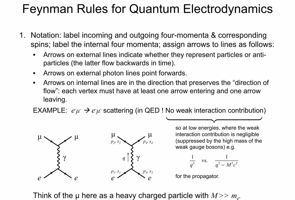
1.  Notation: label incoming and outgoing four-momenta & corresponding spins; label the internal four momenta; assign arrows to lines as follows: •  Arrows on external lines indicate whether they represent particles or anti-

particles (the latter flow backwards in time). •  Arrows on external photon lines point forwards. •  Arrows on internal lines are in the direction that preserves the “direction of

flow”: each vertex must have at least one arrow entering and one arrow leaving.

EXAMPLE: e-µ- e-µ- scattering (in QED ! No weak interaction contribution)

e e

µ µ

γ

e e

µ µ

γ

p1, s1 p3, s3

p2, s2 p4, s4

q

1q2 vs.

1q2 − M 2c2

so at low energies, where the weak interaction contribution is negligible (suppressed by the high mass of the weak gauge bosons) e.g.

for the propagator.

Think of the µ here as a heavy charged particle with M >> me.

2.  External Lines: contribute factors to M as follows:

•  electrons incoming outgoing •  positrons incoming outgoing •  photons incoming outgoing

3.  Vertices: each vertex contributes a factor of (photon is spin-1). (here my g is Griffiths ).

3.  Propagators: each internal line contributes a factor of:

•  electrons and positrons

•  photons

Feynman Rules for QED cont’d

u u ≡ u✝γ 0

v v ≡ v ✝γ 0

ε µ

εµ*

⎫⎬⎭

polarization vectors: see § 7.4

igγµ

ge ≡ e 4π / c = 4πα

i γ µqµ + mc( )q2 − m2c2

−i

gµν

q2

[ e.g. internal fermion line ]

e.g. fermion

e.g. anti-fermion

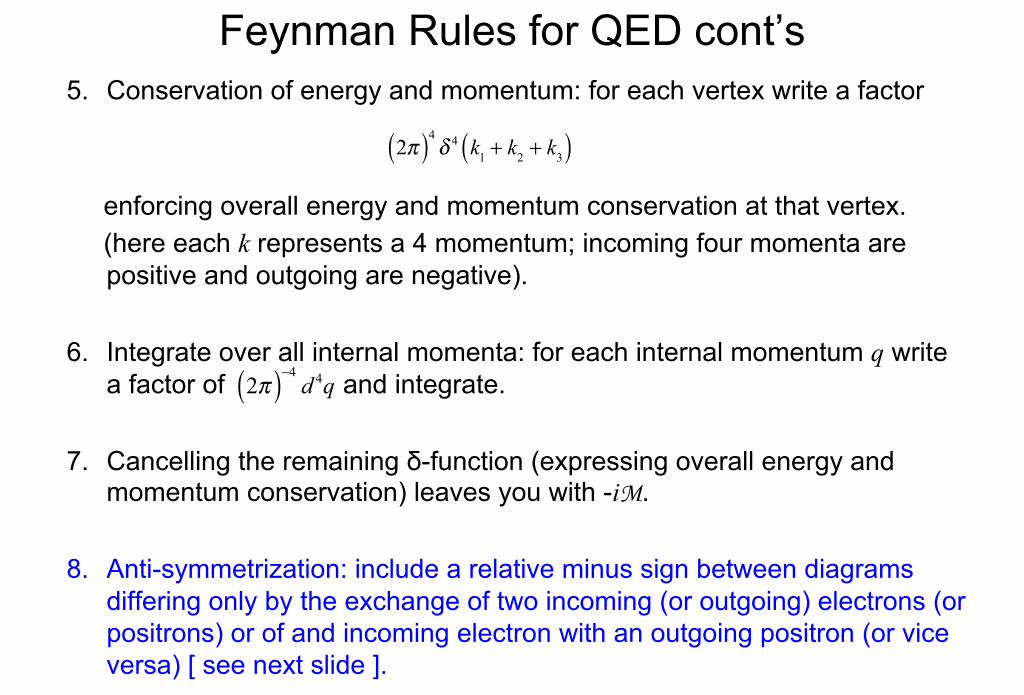
Feynman Rules for QED cont’s 5.  Conservation of energy and momentum: for each vertex write a factor

enforcing overall energy and momentum conservation at that vertex. (here each k represents a 4 momentum; incoming four momenta are

positive and outgoing are negative).

6.  Integrate over all internal momenta: for each internal momentum q write a factor of and integrate.

7.  Cancelling the remaining δ-function (expressing overall energy and momentum conservation) leaves you with -iM.

8.  Anti-symmetrization: include a relative minus sign between diagrams differing only by the exchange of two incoming (or outgoing) electrons (or positrons) or of and incoming electron with an outgoing positron (or vice versa) [ see next slide ].

2π( )4

δ 4 k1 + k2 + k3( )

2π( )−4

d 4q

Anti-symmetrization of QED diagrams Recall the ABC model scattering process AABB. There are two diagrams that contribute at lowest order:

We summed the amplitudes for these two diagrams to get the total amplitude (so, with a relative positive sign).

For fermions the relative sign between such diagrams is negative. p1, s1

p2, s2 p3, s3

p4, s4 p1, s1

p2, s2 p3, s3

p4, s4 _

Here for e−e− → e−e−

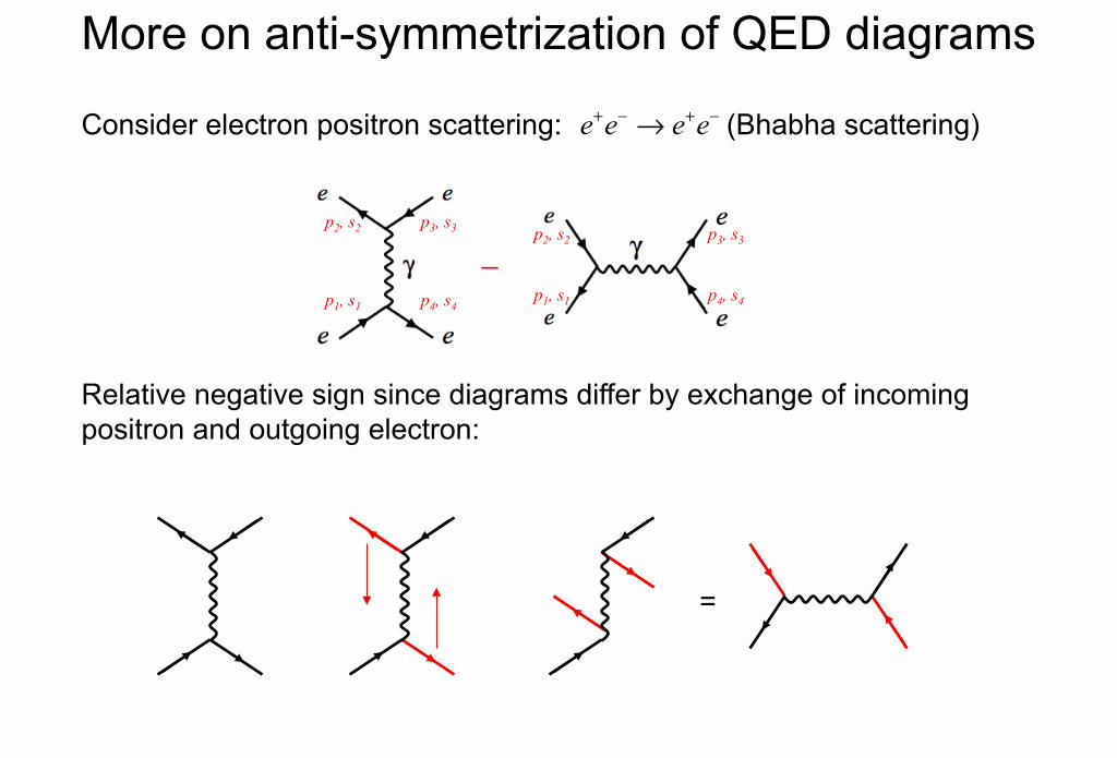
More on anti-symmetrization of QED diagrams

p1, s1

p2, s2 p3, s3

p4, s4 p1, s1

p2, s2 p3, s3

p4, s4

_

Consider electron positron scattering: (Bhabha scattering) e+e− → e+e−

Relative negative sign since diagrams differ by exchange of incoming positron and outgoing electron:

=

Electron-Muon Scattering in QED

Now back to scattering in QED: e−µ− → e−µ−

We had: Now apply Feynman rules to obtain M.

e e

µ µ

γ

p1, s1 p3, s3

p2, s2 p4, s4

q

Procedure is to write down terms working backwards in time along each fermion line:

electron line: u s3( ) p3( ) igγ

µ

u s1( ) p1( )

2π( )4δ 4 p1 − p3 − q( )

outgoing electron spinor

vertex coupling

incoming electron spinor

δ-function for conservation of energy and momentum at electron vertex.

muon line: u s4( ) p4( ) igγ ν u s2( ) p2( ) 2π( )4

δ 4 p2 + q − p4( )

Electron-Muon Scattering cont’d

e e

µ µ

γ

p1, s1 p3, s3

p2, s2 p4, s4

q

∫ u p3( ) igγ µ u p1( ) 2π( )4

δ 4 p1 − p3 − q( )⎡⎣⎢

⎤⎦⎥−igµν

q2 u p4( ) igγ ν u p2( ) 2π( )4δ 4 p2 + q − p4( )⎡

⎣⎢⎤⎦⎥

d 4q

2π( )4

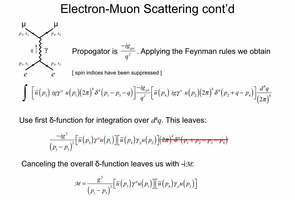
Propogator is . Applying the Feynman rules we obtain

−igµν

q2

[ spin indices have been suppressed ]

Use first δ-function for integration over d4q. This leaves:

−ig 2

p1 − p3( )2 u p3( )γ µu p1( )⎡⎣ ⎤⎦ u p4( )γ µu p2( )⎡⎣ ⎤⎦ 2π( )4δ 4 p1 + p2 − p3 − p4( )

Canceling the overall δ-function leaves us with -iM:

M =g 2

p1 − p3( )2 u p3( )γ µu p1( )⎡⎣ ⎤⎦ u p4( )γ µu p2( )⎡⎣ ⎤⎦

Electron-Muon Scattering cont’d

e e

µ µ

γ

p1, s1 p3, s3

p2, s2 p4, s4

q

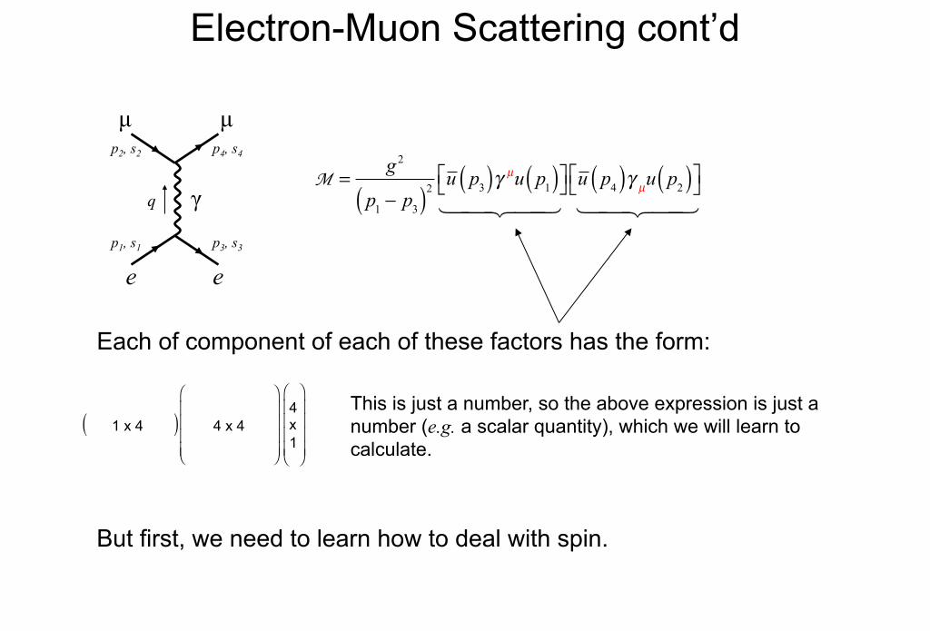
M =g 2

p1 − p3( )2 u p3( )γ µu p1( )⎡⎣ ⎤⎦ u p4( )γ µu p2( )⎡⎣ ⎤⎦

Each of component of each of these factors has the form:

( )⎛

⎝

⎜⎜⎜⎜

⎞

⎠

⎟⎟⎟⎟

⎛

⎝

⎜⎜⎜⎜

⎞

⎠

⎟⎟⎟⎟

1 x 4 4 x 4 4 x 1

This is just a number, so the above expression is just a number (e.g. a scalar quantity), which we will learn to calculate.

But first, we need to learn how to deal with spin.

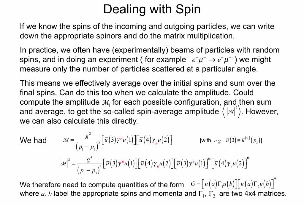
Dealing with Spin If we know the spins of the incoming and outgoing particles, we can write down the appropriate spinors and do the matrix multiplication.

In practice, we often have (experimentally) beams of particles with random spins, and in doing an experiment ( for example ) we might measure only the number of particles scattered at a particular angle.

This means we effectively average over the initial spins and sum over the final spins. Can do this too when we calculate the amplitude. Could compute the amplitude Mi for each possible configuration, and then sum and average, to get the so-called spin-average amplitude . However, we can also calculate this directly.

e−µ− → e−µ−

M

2

M =g 2

p1 − p3( )2 u 3( )γ µu 1( )⎡⎣ ⎤⎦ u 4( )γ µu 2( )⎡⎣ ⎤⎦ [with, e.g. ] u 3( ) ≡ u s3( ) p3( )

M2=

g 4

p1 − p3( )4 u 3( )γ µu 1( )⎡⎣ ⎤⎦ u 4( )γ µu 2( )⎡⎣ ⎤⎦ u 3( )γ νu 1( )⎡⎣ ⎤⎦∗

u 4( )γ νu 2( )⎡⎣ ⎤⎦*

We therefore need to compute quantities of the form where a, b label the appropriate spins and momenta and Γ1, Γ2 are two 4x4 matrices.

G ≡ u a( )Γ1u b( )⎡⎣ ⎤⎦ u a( )Γ2u b( )⎡⎣ ⎤⎦

*

We had

Spin-averaging cont’d We need to evaluate factors like

G ≡ u a( )Γ1u b( )⎡⎣ ⎤⎦ u a( )Γ2u b( )⎡⎣ ⎤⎦

*

Note that is just a number (or a 1x1 matrix), so u a( )Γ2u b( )⎡⎣ ⎤⎦

u a( )Γ2u b( )⎡⎣ ⎤⎦

*= u a( )Γ2u b( )⎡⎣ ⎤⎦

✝

= u a( )✝ γ 0 Γ2u b( )⎡

⎣⎢⎤⎦⎥✝

= u b( )✝ Γ2

✝γ 0✝u a( )

= u b( )✝ γ 0γ 0( )Γ2

✝γ 0u a( ) γ0γ 0 = 1, γ 0✝ = γ 0[since ]

= u b( )γ 0Γ2

✝γ 0u a( ) = u b( )Γ2u a( ) Γ2 ≡ γ 0Γ2✝γ 0where

G ≡ u a( )Γ1u b( )⎡⎣ ⎤⎦ u a( )Γ2u b( )⎡⎣ ⎤⎦

*= u a( )Γ1u b( )⎡⎣ ⎤⎦ u b( )Γ2u a( )⎡⎣ ⎤⎦So

Remember,we have to sum this quantity over all possible spins. Write it in this form to take advantage of the completeness relation for the spinors, when performing this spin sum:

u s( )s=1,2∑ u s( ) = γ µ pµ + mc

v s( )s=1,2∑ v s( ) = γ µ pµ − mc

⎫

⎬⎪

⎭⎪

See eqn 7.99 and problem 7.24

Summing G over the spin orientations of particle b we obtain

G

b− spins∑ = u a( )Γ1 u sb( )

sb =1,2∑ pb( )u sb( ) pb( )⎧

⎨⎪

⎩⎪

⎫⎬⎪

⎭⎪Γ2u a( )

= u a( )Γ1 γ µ pbµ + mbc( )Γ2u a( )

= u a( )Γ1 /pb + mbc( )Γ2u a( ) [ where /pb ≡ γ µ pbµ : in general /a ≡ γ µaµ ]

= u a( )Qu a( ) [with Q = Γ1 /pb + mbc( )Γ2 ]

Need to also sum over possible spin states of particle a:

G

b− spins∑

⎛

⎝⎜⎞

⎠⎟a− spins∑ = u sa( )

sa =1,2∑ pa( )Qu sa( ) pa( )

[ Note that Q is still just a 4x4 matrix ]

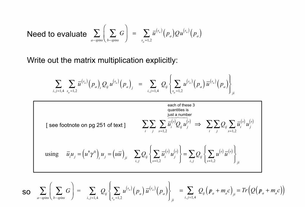
Need to evaluate

Gb− spins∑

⎛

⎝⎜⎞

⎠⎟a− spins∑ = u sa( )

sa =1,2∑ pa( )Qu sa( ) pa( )

Write out the matrix multiplication explicitly:

u sa( )sa =1,2∑ pa( )i

Qij u sa( ) pa( ) ji, j=1,4∑ = Qij u sa( )

sa =1,2∑ pa( ) u sa( ) pa( )⎧

⎨⎪

⎩⎪

⎫⎬⎪

⎭⎪i, j=1,4∑

ji

Qij u sa( )sa =1,2∑ pa( ) u sa( ) pa( )⎧

⎨⎪

⎩⎪

⎫⎬⎪

⎭⎪i, j=1,4∑

ji = Qij /pa + mac( ) ji

i, j=1,4∑

G

b− spins∑

⎛

⎝⎜⎞

⎠⎟a− spins∑ =so

= Tr Q /pa + mac( )( )

using uiu j = u✝γ 0( )

iu j = uu( ) ji

Qij ui

s( )s=1,2∑ uj

s( )⎧⎨⎪

⎩⎪

⎫⎬⎪

⎭⎪i, j∑ = Qij u s( )

s=1,2∑ u s( )⎧

⎨⎪

⎩⎪

⎫⎬⎪

⎭⎪i, j∑

ji

ui

s( )s=1,2∑ Qij u j

s( )j∑ ⇒

i∑ Qij

j∑

i∑ ui

s( )s=1,2∑ uj

s( )

each of these 3 quantities is just a number

[ see footnote on pg 251 of text ]

uu = uu✝γ 0 =

u1

u2

u3

u4

⎛

⎝

⎜⎜⎜⎜⎜

⎞

⎠

⎟⎟⎟⎟⎟

u1* u2

* u3* u4

*( )1 0 0 00 1 0 00 0 −1 00 0 0 −1

⎛

⎝

⎜⎜⎜⎜

⎞

⎠

⎟⎟⎟⎟

=

u1

u2

u3

u4

⎛

⎝

⎜⎜⎜⎜⎜

⎞

⎠

⎟⎟⎟⎟⎟

u1* u2

* −u3* −u4

*( ) =u1u1

* u1u2* −u1u3

* −u1u4*

u2u1* u2u2

* −u2u3* −u2u4

*

u3u1* u3u2

* −u3u3* −u3u4

*

u4u1* u4u2

* −u4u3* −u4u4

*

⎛

⎝

⎜⎜⎜⎜⎜⎜

⎞

⎠

⎟⎟⎟⎟⎟⎟

i = 1, j = 3 ⇒ uiu j = u1

*u3 = uu( )3,1

uiu j = u✝γ 0( )iu j = u1

* u2* u3

* u4*( )

1 0 0 00 1 0 00 0 −1 00 0 0 −1

⎛

⎝

⎜⎜⎜⎜

⎞

⎠

⎟⎟⎟⎟

⎧

⎨⎪⎪

⎩⎪⎪

⎫

⎬⎪⎪

⎭⎪⎪

i

u j =

ui*uj (i = 1,2)

−ui*uj (i = 3,4)

i = 3, j = 1 ⇒ uiu j = − u3

*u1 = uu( )1,3

uiu j = u✝γ 0( )

iu j = uu( ) jiShow that (which we used on the previous slide).

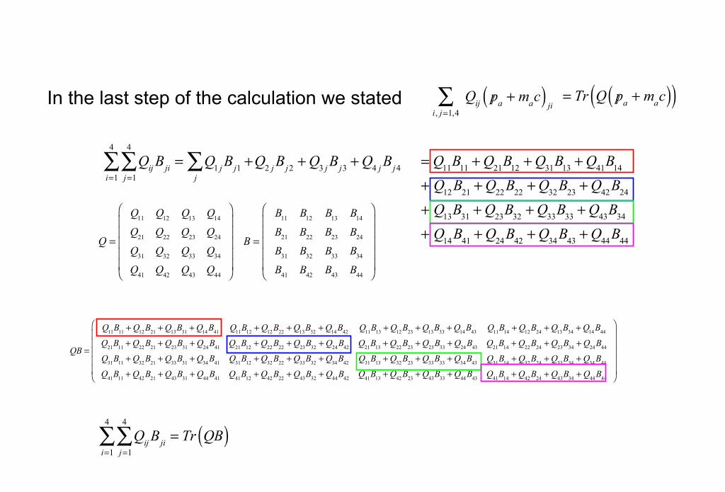
Qij /pa + mac( ) ji

i, j=1,4∑

= Tr Q /pa + mac( )( )In the last step of the calculation we stated

Qij Bji = Q1 j Bj1 +

j∑

j=1

4

∑i=1

4

∑ Q2 j Bj2 + Q3 j Bj3 + Q4 j Bj4

= Q11B11 + Q21B12 + Q31B13 + Q41B14

+ Q12 B21 + Q22 B22 + Q32 B23 + Q42 B24

+ Q13B31 + Q23B32 + Q33B33 + Q43B34

+ Q14 B41 + Q24 B42 + Q34 B43 + Q44 B44

QB =

Q11B11 + Q12 B21 + Q13B31 + Q14 B41 Q11B12 + Q12 B22 + Q13B32 + Q14 B42 Q11B13 + Q12 B23 + Q13B33 + Q14 B43 Q11B14 + Q12 B24 + Q13B34 + Q14 B44




⎛

⎝

⎜⎜⎜⎜⎜

⎞

⎠

⎟⎟⎟⎟⎟

Q =

Q11 Q12 Q13 Q14

Q21 Q22 Q23 Q24

Q31 Q32 Q33 Q34

Q41 Q42 Q43 Q44

⎛

⎝

⎜⎜⎜⎜⎜

⎞

⎠

⎟⎟⎟⎟⎟

B =

B11 B12 B13 B14

B21 B22 B23 B24

B31 B32 B33 B34

B41 B42 B43 B44

⎛

⎝

⎜⎜⎜⎜⎜

⎞

⎠

⎟⎟⎟⎟⎟

Qij Bji = Tr QB( )

j=1

4

∑i=1

4

∑

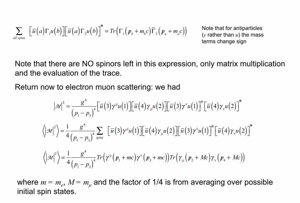
all spins∑ u a( )Γ1u b( )⎡⎣ ⎤⎦ u a( )Γ2u b( )⎡⎣ ⎤⎦

*= Tr Γ1 /pb + mbc( )Γ2 /pa + mac( )( )

Note that there are NO spinors left in this expression, only matrix multiplication and the evaluation of the trace.

Note that for antiparticles (v rather than u) the mass terms change sign

Return now to electron muon scattering: we had

M2=

g 4

p1 − p3( )4 u 3( )γ µu 1( )⎡⎣ ⎤⎦ u 4( )γ µu 2( )⎡⎣ ⎤⎦ u 3( )γ νu 1( )⎡⎣ ⎤⎦∗

u 4( )γ νu 2( )⎡⎣ ⎤⎦*

M2

=14

g 4

p1 − p3( )4spins∑ u 3( )γ µu 1( )⎡⎣ ⎤⎦ u 4( )γ µu 2( )⎡⎣ ⎤⎦ u 3( )γ νu 1( )⎡⎣ ⎤⎦

∗u 4( )γ νu 2( )⎡⎣ ⎤⎦

*

M2

=14

g 4

p1 − p3( )4 Tr γ µ /p1 + mc( )γ ν /p3 + mc( )( )Tr γ µ /p2 + Mc( )γ ν /p4 + Mc( )( )

where m = me, M = mµ and the factor of 1/4 is from averaging over possible initial spin states.

Griffiths §7.7 lists many identities that are needed for the evaluation of the types of traces we will encounter. Here list only those that are relevant to the current calculation:

1. Tr A+ B( ) = Tr A( ) + Tr B( )

2. Tr αA( ) = αTr A( )

10. The trace of the product of an odd number of γ matrices is 0

12. Tr γ µγ ν( ) = 4gµν

13. Tr γ µγ νγ λγ σ( ) = 4 gµνgλσ − gµλgνσ + gµσ gνλ( )

Tr γ µ /p1 + mc( )γ ν /p3 + mc( )( ) 1,2⎯ →⎯ Tr γ µ /p1γ

ν /p3( ) + mc Tr γ µ /p1γν( ) + Tr γ µγ ν /p3( )⎡

⎣⎤⎦ + mc( )2

Tr γ µγ ν( )= 0 by rule 10.

= Tr γ µ /p1γ

ν /p3( ) + mc( )2Tr γ µγ ν( )

Tr γ µ /p1γ

ν /p3( ) + mc( )2Tr γ µγ ν( )

Tr γ µ /p1γ

ν /p3( ) = p1( )λ p3( )σ Tr γ µγ λγ νγ σ( ) [since each element of p1 or p3 is just a number]

= p1( )λ p3( )σ 4 gµλgνσ − gµνgλσ + gµσ gλν( ) [using rule 13]

= 4 p1

µ p3ν − gµν p1 ⋅ p3( ) + p3

µ p1ν( ) [simply contracting the indices]

mc( )2

Tr γ µγ ν( ) = 4 mc( )2gµν [using rule 12]

Tr γ µ /p1 + mc( )γ ν /p3 + mc( )( ) = 4 p1

µ p3ν + p3

µ p1ν + gµν mc( )2

− p1 ⋅ p3( )⎛⎝

⎞⎠

The other trace in our calculation is the same, but with mM, 12, 3 4 and the greek indices lowered; that is,

Tr γ µ /p2 + Mc( )γ ν /p4 + Mc( )( ) = 4 p2µ p4ν + p4µ p2ν + gµν Mc( )2

− p2 ⋅ p4( )⎛⎝

⎞⎠

M2

=14

g 4

p1 − p3( )4 Tr γ µ /p1 + mc( )γ ν /p3 + mc( )( )Tr γ µ /p2 + Mc( )γ ν /p4 + Mc( )( )

M2

=14

g 4

p1 − p3( )4 4 p1µ p3

ν + p3µ p1

ν − gµν mc( )2− p1 ⋅ p3( )⎛

⎝⎞⎠{ } 4 p2µ p4ν + p4µ p2ν − gµν Mc( )2

− p2 ⋅ p4( )⎛⎝

⎞⎠{ }

M2

= 4g 4

p1 − p3( )4 p1µ p3

ν + p3µ p1

ν − gµν mc( )2− p1 ⋅ p3( )⎛

⎝⎞⎠ p2µ p4ν + p4µ p2ν − gµν Mc( )2

− p2 ⋅ p4( )⎛⎝

⎞⎠

M2

= 4g 4

p1 − p3( )4 p1µ p3

ν p2µ p4ν + p1µ p3


νgµν Mc( )2− p2 ⋅ p4( ){

+ p3µ p1



νgµν Mc( )2− p2 ⋅ p4( )

+ p2µ p4νgµν mc( )2− p1 ⋅ p3( ) + p4µ p2νgµν mc( )2

− p1 ⋅ p3( ) +gµν mc( )2

− p1 ⋅ p3( )gµν Mc( )2− p2 ⋅ p4( ) }

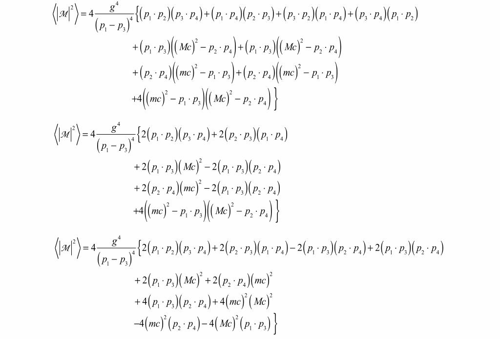
M2

= 4g 4

p1 − p3( )4 p1 ⋅ p2( ){ p3 ⋅ p4( ) + p1 ⋅ p4( ) p2 ⋅ p3( ) + p3 ⋅ p2( ) p1 ⋅ p4( ) + p3 ⋅ p4( ) p1 ⋅ p2( )

+ p1 ⋅ p3( ) Mc( )2− p2 ⋅ p4( ) + p1 ⋅ p3( ) Mc( )2

− p2 ⋅ p4( ) + p2 ⋅ p4( ) mc( )2

− p1 ⋅ p3( ) + p2 ⋅ p4( ) mc( )2− p1 ⋅ p3( )

+4 mc( )2− p1 ⋅ p3( ) Mc( )2

− p2 ⋅ p4( ) }

M2

= 4g 4

p1 − p3( )4 2 p1 ⋅ p2( ){ p3 ⋅ p4( ) + 2 p2 ⋅ p3( ) p1 ⋅ p4( )

+ 2 p1 ⋅ p3( ) Mc( )2− 2 p1 ⋅ p3( ) p2 ⋅ p4( )

+ 2 p2 ⋅ p4( ) mc( )2− 2 p1 ⋅ p3( ) p2 ⋅ p4( )

+4 mc( )2− p1 ⋅ p3( ) Mc( )2

− p2 ⋅ p4( ) }

M2

= 4g 4

p1 − p3( )4 2 p1 ⋅ p2( ){ p3 ⋅ p4( ) + 2 p2 ⋅ p3( ) p1 ⋅ p4( ) − 2 p1 ⋅ p3( ) p2 ⋅ p4( ) + 2 p1 ⋅ p3( ) p2 ⋅ p4( )

+ 2 p1 ⋅ p3( ) Mc( )2+ 2 p2 ⋅ p4( ) mc( )2

+ 4 p1 ⋅ p3( ) p2 ⋅ p4( ) + 4 mc( )2Mc( )2

−4 mc( )2p2 ⋅ p4( ) − 4 Mc( )2

p1 ⋅ p3( ) }

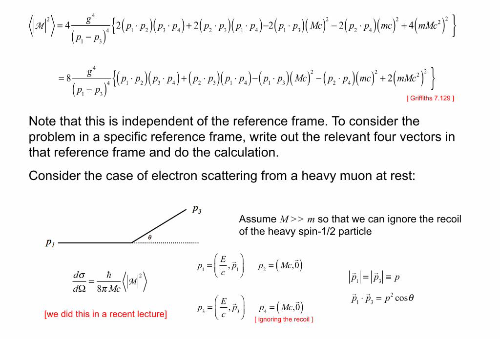
M2

= 4g 4

p1 − p3( )4 2 p1 ⋅ p2( ){ p3 ⋅ p4( ) + 2 p2 ⋅ p3( ) p1 ⋅ p4( )−2 p1 ⋅ p3( ) Mc( )2− 2 p2 ⋅ p4( ) mc( )2

+ 4 mMc2( )2 }

= 8g 4

p1 − p3( )4 p1 ⋅ p2( ){ p3 ⋅ p4( ) + p2 ⋅ p3( ) p1 ⋅ p4( )− p1 ⋅ p3( ) Mc( )2− p2 ⋅ p4( ) mc( )2

+ 2 mMc2( )2 }[ Griffiths 7.129 ]

Note that this is independent of the reference frame. To consider the problem in a specific reference frame, write out the relevant four vectors in that reference frame and do the calculation.

Consider the case of electron scattering from a heavy muon at rest:

Assume M >> m so that we can ignore the recoil of the heavy spin-1/2 particle

dσdΩ

=

8π McM

2

[we did this in a recent lecture]

p1 =Ec

, p1

⎛⎝⎜

⎞⎠⎟

p2 = Mc,0( )

p3 =Ec

, p3

⎛⎝⎜

⎞⎠⎟

p4 = Mc,0( )

[ ignoring the recoil ]

p1 = p3 ≡ p

p1 ⋅p3 = p2 cosθ

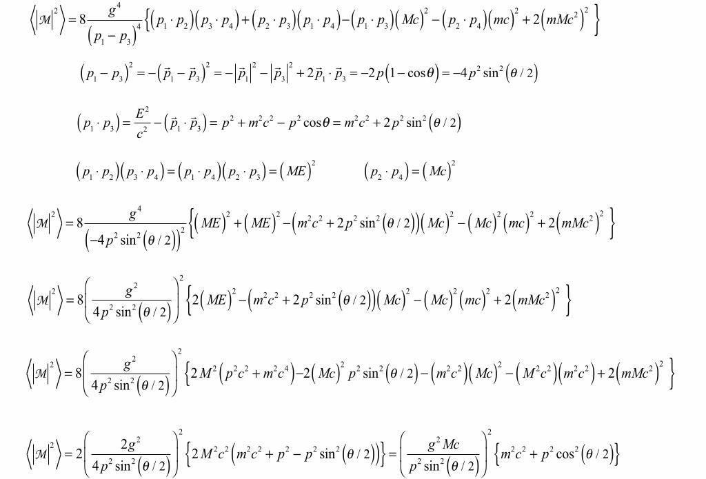
M2

= 8g 4

p1 − p3( )4 p1 ⋅ p2( ){ p3 ⋅ p4( ) + p2 ⋅ p3( ) p1 ⋅ p4( )− p1 ⋅ p3( ) Mc( )2− p2 ⋅ p4( ) mc( )2

+ 2 mMc2( )2 }

p1 − p3( )2= − p1 −

p3( )2= − p1

2− p3

2+ 2 p1 ⋅

p3 = −2 p 1− cosθ( ) = −4 p2 sin2 θ / 2( )

p1 ⋅ p3( ) = E2

c2 − p1 ⋅p3( ) = p2 + m2c2 − p2 cosθ = m2c2 + 2 p2 sin2 θ / 2( )

p1 ⋅ p2( ) p3 ⋅ p4( ) = p1 ⋅ p4( ) p2 ⋅ p3( ) = ME( )2

p2 ⋅ p4( ) = Mc( )2

M2

= 8g 4

−4 p2 sin2 θ / 2( )( )2 ME( )2{ + ME( )2− m2c2 + 2 p2 sin2 θ / 2( )( ) Mc( )2

− Mc( )2mc( )2

+ 2 mMc2( )2 }

M

2= 8

g 2

4 p2 sin2 θ / 2( )⎛

⎝⎜

⎞

⎠⎟

2

2 ME( )2{ − m2c2 + 2 p2 sin2 θ / 2( )( ) Mc( )2− Mc( )2

mc( )2+ 2 mMc2( )2 }

M

2= 8

g 2

4 p2 sin2 θ / 2( )⎛

⎝⎜

⎞

⎠⎟

2

2M 2 p2c2 + m2c4( ){ −2 Mc( )2p2 sin2 θ / 2( ) − m2c2( ) Mc( )2

− M 2c2( ) m2c2( ) + 2 mMc2( )2 }

M

2= 2

2g 2

4 p2 sin2 θ / 2( )⎛

⎝⎜

⎞

⎠⎟

2

2M 2c2 m2c2 + p2 − p2 sin2 θ / 2( )( ){ } = g 2 Mcp2 sin2 θ / 2( )

⎛

⎝⎜

⎞

⎠⎟

2

m2c2 + p2 cos2 θ / 2( ){ }

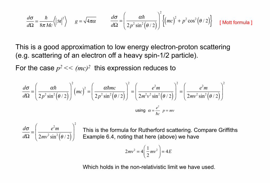
This is a good approximation to low energy electron-proton scattering (e.g. scattering of an electron off a heavy spin-1/2 particle).

For the case p2 << (mc)2 this expression reduces to

dσdΩ

=α

2 p2 sin2 θ / 2( )⎛

⎝⎜

⎞

⎠⎟

2

mc( )2=

αmc2 p2 sin2 θ / 2( )

⎛

⎝⎜

⎞

⎠⎟

2

=e2m

2m2v2 sin2 θ / 2( )⎛

⎝⎜

⎞

⎠⎟

2

=e2m

2mv2 sin2 θ / 2( )⎛

⎝⎜

⎞

⎠⎟

2

α =

e2

c p = mvusing

dσdΩ

=e2m

2mv2 sin2 θ / 2( )⎛

⎝⎜

⎞

⎠⎟

2

This is the formula for Rutherford scattering. Compare Griffiths Example 6.4, noting that here (above) we have

Which holds in the non-relativistic limit we have used.

2mv2 = 4

12

mv2⎛⎝⎜

⎞⎠⎟= 4E

dσdΩ

=α

2 p2 sin2 θ / 2( )⎛

⎝⎜

⎞

⎠⎟

2

mc( )2+ p2 cos2 θ / 2( ){ }

dσdΩ

=

8π McM

2

g = 4πα [ Mott formula ]

phy489 lecture 15 - university of toronto

Documents