PH

YS

ICS

LA

B M

AN

UA

L E

NG

INE

ER

ING

SC

IEN

CE

& P

HY

SIC

S D

EP

AR

TM

EN

T

C O L L E G E O F S T A T E N I S L A N D

C I T Y U N I V E R S I T Y O F N E W Y O R K

PHY 116

“The important thing in science is not so much to obtain new facts as to discover new ways of thinking about them.” --Sir William Lawrence Bragg

COLLEGE OF STATEN ISLAND

PHY 116

PHYSICS LAB MANUAL

ENGINEERING SCIENCE & PHYSICS DEPARTMENT

CITY UNIVERSITY OF NEW YORK

ENGINEERING SCIENCE & PHYSICS DEPARTMENT

PHYSICS LABORATORY EXT 2978, 4N-214/4N-215

ENGINEERING SCIENCE & PHYSICS DEPARTMENT

PHYSICS LABORATORY EXT 2978, 4N-214/4N-215

LABORATORY RULES

1. No eating or drinking in the laboratory premises.

2. The use of cell phones is not permitted.

3. Computers are for experiment use only. No web surfing, reading e-mail,

instant messaging or computer games allowed.

4. When finished using a computer log-off and put your keyboard and mouse

away.

5. Arrive on time otherwise equipment on your station will be removed.

6. Bring a scientific calculator for each laboratory session.

7. Have a hard copy of your laboratory report ready to submit before you enter

the laboratory.

8. Some equipment will be required to be signed out and checked back in. The

rest of the equipment should be returned as directed by the technician. All

equipment must be treated with care and caution. No markings or writing is

allowed on any piece of equipment or tables. Remember, you are responsible

for the equipment you use during an experiment.

9. After completing the experiment and, if needed, putting away equipment,

check that your station is clean and clutter free and push in your chair.

10. Before leaving the laboratory premises, make sure that you have all your

belongings with you. The lab is not responsible for any lost items.

Your cooperation in abiding by these rules will be highly appreciated.

Thank You.

The Physics Laboratory Staff

ENGINEERING SCIENCE & PHYSICS DEPARTMENT

PHYSICS LABORATORY EXT 2978, 4N-214/4N-215

10 ESSENTIALS of

writing laboratory reports ALL students must comply with

1. No report is accepted from a student who didn’t actually participate in the

experiment.

2. Despite that the actual lab is performed in a group, a report must be individually

written. Photocopies or plagiaristic reports will not be accepted and zero grade

will be issued to all parties.

3. The laboratory report should have a title page giving the name and number of

the experiment, the student's name, the class, and the date of the experiment.

The laboratory partner’s name must be included on the title page, and it should

be clearly indicated who the author and who the partner is.

4. Each section of the report, that is, “objective”, “theory background”, etc.,

should be clearly labeled. The data sheet collected by the author of the report

during the lab session with instructor’s signature must be included – no report

without such a data sheet indicating that the author has actually performed the

experiment is to be accepted.

5. Paper should be 8 ½” x 11”. Write on one side only using word-processing

software. Ruler and compass should be used for diagrams. Computer graphing

is also accepted.

6. Reports should be stapled together.

7. Be as neat as possible in order to facilitate reading your report.

8. Reports are due one week following the experiment. No reports will be

accepted after the "Due-date" without penalty as determined by the instructor.

9. No student can pass the course unless he or she has turned in a set of laboratory

reports required by the instructor.

10. The student is responsible for any further instruction given by the instructor.

PHY 116

TABLE OF CONTENTS

The laboratory instructor, in order to adjust to the lecture schedule or personal preference, maysubstitute any of the experiments below with supplementary experiments.

1. LABORATORY REPORT FORMAT AND DATA ANALYSIS........................................1

2. VERNIER CALIPER - MICROMETER CALIPER............................................................9

3. MASS, MASS DENSITY, SPECIFIC GRAVITY..............................................................15

4. ADDITION OF VECTORS................................................................................................21

5. MOTION OF A BODY IN FREE FALL............................................................................25

6. HORIZONTAL PROJECTILE MOTION...........................................................................31

7. EQUILIBRIUM OF A RIGID BODY.................................................................................33

8. FRICTION...........................................................................................................................39

9. NEWTON’S SECOND LAW.............................................................................................41

10. SIMPLE PENDULUM.........................................................................................................47

11. CENTRIPETAL FORCE....................................................................................................49

12. WORK AND KINETIC ENERGY......................................................................................51

13. CONSERVATION OF MOMENTUM................................................................................53

14. ROTATIONAL MOTION AND MOMENT OF INERTIA.................................................55

SUPPLEMENTARY EXPERIMENTS

15. DENSITY AND ARCHIMEDES’ PRINCIPLE...................................................................61

16. COLLISION IN TWO DIMENSIONS................................................................................65

17. VIBRATIONS OF A SPRING................................................................................................67

18. CALORIMETRY.................................................................................................................69

19. SOUND WAVES..................................................................................................................71

20. DETERMINING g ON AN INCLINE..............................................................................75

21. PENDULUM STUDIES......................................................................................................79

APPENDIX:

A1 GRAPHICAL ANALYSIS 3.4 - FINDING THE BEST FIT.................................................85

A2 TECHNICAL NOTES ON VERNIER LABQUEST INTERFACE...................................89

A3 TECHNICAL NOTES ON SENSORS AND PROBES.....................................................93

All diagrams and tables created by Jackeline S. Figueroa, Senior CLT.Except for diagrams on pages 9-12, 21(Fig. 1) and 87-96

1

LABORATORY REPORTS FORMAT AND PRESENTATION OF DATA The Laboratory Report should contain the following information: 1. Objective of the lab; 2. Physical Principles and laws tested and used; 3. Explanation (rather than a description) of the procedure; 4. Laboratory Data: arranged in tabular form with labeled rows and columns. Note that

the data sheet must be signed by the instructor in the presence of the student when the experiment is completed;

5. Computations and graphs of the main quantities and their errors; 6. Summary of Results which includes: discussion of the results and their errors as well as

a conclusion based on this discussion as to what extent the lab objective is achieved. 7. Answers to all questions. I. ERRORS OF OBSERVATION

1. Blunders:

Every measurement is subject to error. Obviously, one should know how to reduce or minimize error as much as possible. The commonest and simplest type of error to remove is a blunder, due to carelessness, in making a measurement. Blunders are diminished by experience and the repetition of observations.

2. Personal Errors:

These are errors peculiar to a particular observer. For example beginners very often try to fit measurement to some preconceived notion. Also, the beginner is often prejudiced in favor of his first observation.

3. Systematic Errors:

Are errors associated with the particular instruments or technique of measurement being used. Suppose we have a book which is 9in. high. We measure its height by laying a ruler against it, with one end of the ruler at the top end of the book. If the first inch of the ruler has been previously cut off, then the ruler is like to tell us that the book is 10in. long. This is a systematic error. If a thermometer immersed in boiling pure water at normal pressure reads 215°F (should be 212°F) it is improperly calibrated; if readings from this thermometer are incorporated into experimental results, a systematic error results.

4. Accidental (or Random) Errors: When measurements are reasonably free from the above sources of error it is found that whenever an instrument is used to the limit its precision, errors occur which cannot be eliminated completely. Such errors are due to the fact that conditions are continually varying imperceptibly. These errors are largely unpredictable and unknown. For example: A small error in judgment on the part of the observer, such as in estimating to tenths the smallest scale divisions. Other causes are

2

unpredictable fluctuations in conditions, such as temperature, illumination, socket voltage or any kind of mechanical vibrations of the equipment being used. The effect of these errors may be mitigated by repeating the measurement several times and taking the average of the readings. There are two ways of estimating the error due to random independent measurements. One way is to calculate the Mean Absolute Deviation and the other is to calculate the Standard deviation. Both methods are discussed in the appendix.

5. Significant Figures:

Every number expressing the result of a measurement or of computations based on measurements should be written with the proper number of "significant figures." The number of significant figures is independent of the position of the decimal point: i.e. 8.448cm, 84.48mm, or 0.08448m has the same number of significant figures. A figure ceased to be a significant when we have no reason to believe, on the basis of measurement made, that the correct result is probably closer to that figure than to the next (higher or lower) figure. In computations, since figures which are not significant in this sense have no place in the final result, they should be dropped to avoid useless labor. e.g. in the measurement of the diameter of a penny we read on the ruler 1.748. Here the last figure is a very rough guess; hence, for computations we use 1.75.

6. Reading error

: Every instrument has a limitation in accuracy. The markings serve as a guide as to that accuracy. We read the instrument to a fraction of the smallest division. As in the diameter of a penny the 8 is an estimated number. We then have to estimate the error in that number. For most applications the reading error can be taken as +/-2. Therefore the experimental value for that measurement is 1.748 +/- 0.002 cm. The reading error may be taken as a constant error for that instrument. The smallest error associated with a measurement is the reading error.

7. Percent ErrorThe Measurement error may be estimated from your measurements a variety of ways. Two simple ways are the standard deviation or the mean absolute error. For most applications the mean absolute error is a good estimate of the measurement error.

: To present the error in a relative manner we calculate the percent error.

Percent Error = |Measurement Error|

Average Value× 100%

8. Percent Difference:

Percent Difference = |Standard Value − Experimental Value|

Standard Value× 100%

In your laboratory work you will often find occasion to compare a value which you have obtained as a result of measurement, with the standard, or generally accepted value. The percent difference is computed as follows:

Note: If Percent Difference (PD) is smaller than Percent Error (PE), you can conclude that the experimental value is consistent with the standard (known) value within estimated errors. If, however, PD is larger than PE, the measured value is inconsistent with the standard (known) one. In other words, if PE is estimated correctly, the measured value can be claimed to be a better estimate of the standard one.

3

II. ANALYSIS OF DATA Every measurement is prone to errors leading to deviations of a measured quantity from one measurement to another. For example, length of a pencil measured several times may come out differently depending on how ruler was applied. Personal blunders due to carelessness are also a source of errors. In general, each particular instrument never gives a result precisely. Many external factors such as, e.g., temperature vary and thereby affect results. Thus, errors of measurements and the associated deviations of measured quantity are an inherent part of the measurement process. Patience and experience are required in order to reduce the errors and the deviations.

In order to evaluate errors the same quantity should be measured at least several times. As an example, the result of such measurements of a length of one object is given in the table below

N 1 2 3 4 5 6 7 8 9 L

[cm] 15.2 15.3 14.9 15.4 15.2 15.1 15.0 14.8 15.2

DL=│L - L │ [cm] 0.1 0.2 0.2 0.3 0.1 0.0 0.1 0.3 0.1

The upper row marked by N gives the number of a particular measurement. The second row shows object’s length obtained during each measurement (for example, the result of the 4th measurement is 15.4 cm). The bottom row gives absolute deviations

|LL|DL −= Eq. 1 of each measurement from the average value (mean value) of the length

cm1.159

)2.158.140.151.152.154.159.143.152.15()L(avgL =++++++++

==

calculated from 9 measurements. In calculating the average, the result must be rounded off so that the number of significant digits is not more than that for each measurement. The mean absolute deviation

DL avg DL= ( ) Eq. 2 indicates how the measured value varied due to all of the factors mentioned above. For our example, DL = 0 2. cm. The final result for the object length is expressed as

L L DL= ± Eq. 3

That is, L cm= ±( . . )151 0 2 . This means that in the measurement of the length the result obtained was between 14.9 cm and 15.3 cm with high certainty.

4

Errors can also be represented as percent error. It is defined as

%100LLD error % ×= Eq. 4

For our example, it is 0 2151 100% 1%

.. ⋅ ≈ . This sort of analysis should be applied to

measurements of other physical quantities.

Sometimes a purpose of the laboratory experiment is to measure a quantity Q whose standard value Qst is well known from theoretical considerations or other measurements. In this case it is important to compare these two quantities Q and Qst in order to make a conclusion on whether your experiment confirmed the value Qst and thereby supported a theoretical concept underlying this value. An important quantity is the percent difference between the measured (mean) value and the standard value:

| | % difference 100%st

st

Q QQ−

= × Eq. 5

We can say that

The errors should always be estimated for the experimental data. Furthermore, any experimental result for which no errors are evaluated is considered as unreliable.

the experiment does confirm the concept within the experimental percent deviation (or percent error), if the percent difference is not bigger than the percent error.

PROPAGATION OF ERRORS

Sometimes a measured quantity is obtained by using some equation, and the question is how to evaluate fractional (or percent) error for such a quantity. For example, density ρ of some material is obtained as the ratio of mass M and volume V: ρ=M/V. While mass can be measured directly by scale, volume is often obtained from measurements of linear dimensions of a rectangular shaped sample as V=L1L2L3. Each four values, M, L1, L2, and L3 have their own errors (mean deviations): The resulting fractional (or % ) error for ρ can be found as a sum of fractional (%) errors of all multiplicative quantities entering the equation.

For our example this means

31 2

1 2 3 1 2 3

, LL LM MM L L L L L L

ρ ρρ

∆∆ ∆∆ ∆= + + + = Eq. 7

M = M� ± ∆M L1 = 𝐿�1 ± ∆𝐿1 L2 = 𝐿�2 ± ∆𝐿2 L3 = 𝐿�3 ± ∆𝐿3

Eq. 6

5

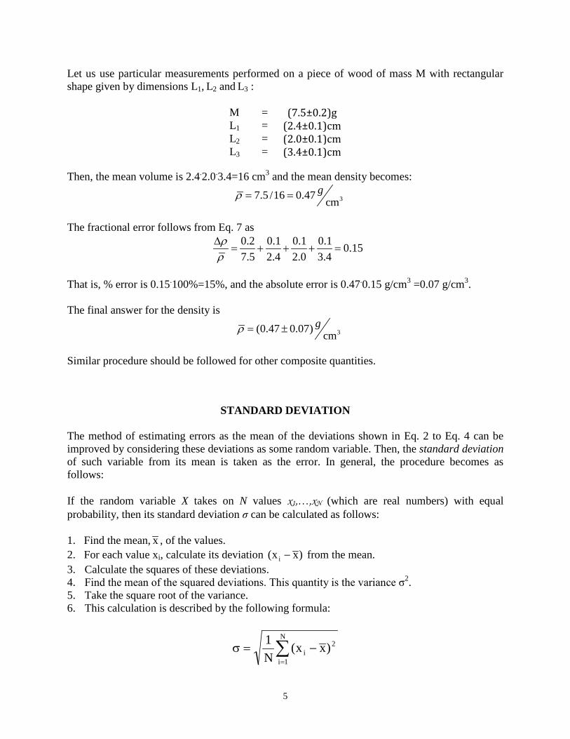
Let us use particular measurements performed on a piece of wood of mass M with rectangular shape given by dimensions L1, L2 and L3 :

Then, the mean volume is 2.4.2.0.3.4=16 cm3 and the mean density becomes:

3 7.5 /16 0.47 cmgρ = =

The fractional error follows from Eq. 7 as

0.2 0.1 0.1 0.1 0.157.5 2.4 2.0 3.4

ρρ∆

= + + + =

That is, % error is 0.15.100%=15%, and the absolute error is 0.47.0.15 g/cm3 =0.07 g/cm3. The final answer for the density is

3 (0.47 0.07) cmgρ = ±

Similar procedure should be followed for other composite quantities.

STANDARD DEVIATION The method of estimating errors as the mean of the deviations shown in Eq. 2 to Eq. 4 can be improved by considering these deviations as some random variable. Then, the standard deviation of such variable from its mean is taken as the error. In general, the procedure becomes as follows:

If the random variable X takes on N values x1,…,xN (which are real numbers) with equal probability, then its standard deviation σ can be calculated as follows:

1. Find the mean, x , of the values. 2. For each value xi, calculate its deviation )xx( i − from the mean. 3. Calculate the squares of these deviations. 4. Find the mean of the squared deviations. This quantity is the variance σ2. 5. Take the square root of the variance. 6. This calculation is described by the following formula:

M = (7.5±0.2)g L1 = (2.4±0.1)cm L2 = (2.0±0.1)cm L3 = (3.4±0.1)cm

∑=

−=σN

1i

2i )xx(

N1

6

where x is the arithmetic mean of the values xi, defined as:

Example: Suppose we wished to find the standard deviation of the data set consisting of the values 3, 7, 7, and 19 Step 1: Find the arithmetic mean (average) of 3, 7, 7, and 19,

94

19773=

+++

Step 2: Find the deviation of each number from the mean,

3 − 9 = -6 7 − 9 = -2 7 − 9 = -2

19 − 9 = 10 Step 3: Square each of the deviations, which amplifies large deviations and makes negative values positive,

(-6)2 = 36 (-2)2 = 4 (-2)2 = 4 102 = 100

Step 4: Find the mean of those squared deviations,

Step 5: Take the non-negative square root of the quotient (converting squared units back to regular units),

So, the standard deviation of the set is 6. This example also shows that, in general, the standard deviation is different from the mean absolute deviation, as calculated in Eq. 2. Specifically for this example the mean deviation is 5. Despite these differences, both methods of estimating errors are acceptable.

∑=

=+++

=N

1ii

N21 xN1

Nx...xx

x

364

1004436=

+++

636 =

7

III. GRAPHICAL REPRESENTATION OF DATA: Some essentials in plotting a graph. 1. Arrange the numbers to be plotted in tabular form if they are not already so arranged.

2. Decide which of the two quantities is to be plotted along the X-axis and which along the Y-axis. It is customary to plot the independent variable along the X-axis and the dependent along the Y.

3. Choose the scale of units for each axis of the graph. That is, decide how many squares of the cross-section plotted along a particular axis. In every case the scales of units for the axes must be so chosen that the completed curve will spread over at least one-half of the full-sized sheet of graph paper. 4. Attach a legend to each axis which will indicate what is plotted along that axis and, in addition, mark the main divisions of each axis in units of the quantity being plotted.

5. Plot each point by indicating its position by a small pencil dot. Then draw a small circle around the dot so that each plotted point will be clearly visible on the completed graph. This circle is drawn with a radius equal to the estimated probable error of that particular measurement (you may use the percent difference when calculable). (See "errors" below).

6. Draw a smooth curve through the plotted points. This curve need not necessarily pass

through any of the points but should have, on the average, as many points on one side of it as it has on the other. The reason for drawing a smooth curve is that it is expected to represent a mathematical relationship between the quantities plotted. Such a mathematical relationship ordinarily will not exhibit any abrupt changes in slope, merely indicates that the measurement is subject to some error. A close fit of the experimental points to the smooth curve shows that the measurement is one of small error.

7. Label the graph. That is, attach a legend which will indicate, at a glance, what the graph purports to show.

8

Fig. 1 - Parts of a Vernier Caliper

Fig. 2 - Dimensions that can be measured with a vernier caliper

ENGLISH SCALE

VERNIER CALIPER - MICROMETER CALIPER

Apparatus:

- Two metal cylinders- One wire- Vernier caliper, 0-150mm, 0.02 least count- Micrometer caliper, 0-25mm, 0.01mm least count

Part I: The Vernier Caliper

When you use English and metric rulers for making measurements it is sometimes difficult to getprecise results. When it is necessary to make more precise linear measurements, you must have amore precise instrument. One such instrument is the vernier caliper. The vernier caliper was introduced in 1631 by Pierre Vernier. It utilizes two graduated scales: amain scale similar to that of a ruler and a especially graduated auxiliary scale, the vernier, that slidesparallel to the main scale and enables readings to be made to a fraction of a division on the mainscale. With this device you can take inside, outside, and depth measurements. Some vernier calipershave two metric scales and two English scales. Others might have the metric scales only.

9

Fig. 3 - Vernier caliper with closed jaws

Notice that if the jaws are closed, the first line at the left end of the vernier, called the zero line orthe index, coincides with the zero line on the main scale (Fig. 2).

The least count can be determined for any type of vernier instrument by dividing the smallestdivision on the main scale by the number of divisions on the vernier scale. The vernier caliper tobe used in the laboratory measurements has a least count 0.02mm. Instructions on how to read themeasurements on this particular model can be found in:

http://www.chicagobrand.com/help/vernier.html

http://www.technologystudent.com/equip1/vernier3.htm

The link below has a caliper simulator, practice with it before the lab session:http://www.stefanelli.eng.br/en/en-vernier-caliper-pachymeter-calliper-simulator-millimeter-02-mm.html

For our experiment will be using a caliper with English and Metric scales. The top main scale isEnglish units and the lower main scale is metric. For our experiment will be concentrating on metriconly. In our model the metric scale is graduated in mm and labeled in cm. That is, each bargraduation on the main scale is 1mm. Every 10th graduation is numbered (10mm). The vernier scaledivides the millimeter by fifty (1/50), marking the 0.02mm (two hundredths of a millimeter), whichis then the least count of the instrument. In other words, each vernier graduation corresponds to0.02mm. Every 5th graduation (0.1mm) is numbered.

Having first determined the least count of the instrument, a measurement may be made by closingthe jaws on the object to be measured and then reading the position where the zero line of the vernierfalls on the main scale (no attempt being made to estimate to a fraction of a main scale division). Wenext note which line on the vernier coincides with a line on the main scale and multiply the numberrepresented by this line (e.g., 0,1,2, etc.) by the least count on the instrument. The product is thenadded to the number already obtained from the main scale. Occasionally, it will be found that no lineon the vernier will coincide with a line on the main scale. Then the average of the two closest linesis used yielding a reading error of approximately 0.01mm. In this case we take the line that mostcoincides.

10

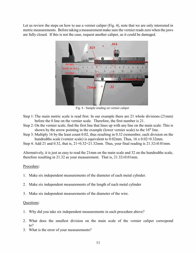
Fig. 4 - Sample reading on vernier caliper

Let us review the steps on how to use a vernier caliper (Fig. 4), note that we are only interested inmetric measurements. Before taking a measurement make sure the vernier reads zero when the jawsare fully closed. If this is not the case, request another caliper, as it could be damaged.

Step 1: The main metric scale is read first. In our example there are 21 whole divisions (21mm)before the 0 line on the vernier scale. Therefore, the first number is 21.

Step 2: On the vernier scale, find the first line that lines up with any line on the main scale. This isshown by the arrow pointing in the example (lower vernier scale) to the 16th line.

Step 3: Multiply 16 by the least count 0.02, thus resulting in 0.32 (remember, each division on thehundredths scale (vernier scale) is equivalent to 0.02mm. Thus, 16 x 0.02=0.32mm.

Step 4: Add 21 and 0.32, that is, 21+0.32=21.32mm. Thus, your final reading is 21.32±0.01mm.

Alternatively, it is just as easy to read the 21mm on the main scale and 32 on the hundredths scale,therefore resulting in 21.32 as your measurement. That is, 21.32±0.01mm.

Procedure:

1. Make six independent measurements of the diameter of each metal cylinder.

2. Make six independent measurements of the length of each metal cylinder

3. Make six independent measurements of the diameter of the wire.

Questions:

1. Why did you take six independent measurements in each procedure above?

2. What does the smallest division on the main scale of the vernier caliper correspond to?

3. What is the error of your measurements?

11

Fig. 5 - Micrometer Caliper

Part II. The Micrometer Caliper:

The micrometer caliper, invented by William Gascoigne in the 17th century, is typically used tomeasure very small thicknesses and diameters of wires and spheres. It consists of a screw of pitch0.5mm, a main scale and another scale engraved around a thimble which rotates with the screw andmoves along the scale on the barrel. The barrel scale is divided into millimeters, on someinstruments, such as ours, a supplementary scale shows half millimeters.

The thimble scale has 50 divisions. Since one complete turn of the thimble will produce an axialmovement of 0.5mm. One scale division movement of the thimble past the axial line of the scale onthe barrel is equivalent to 1/100 times 1.0 equals 0.01mm. Hence readings may be taken directly toone hundredth of a millimeter and by estimation (of tenths of a thimble scale division) to athousandth of a millimeter.

The object to be measured is inserted between the end of the screw (the spindle) and the anvil on theother leg of the frame. The thimble is then rotated until the object is gripped gently. A ratchet at theend of the thimble serves to close the screw on the object with a light and constant force. Thebeginner should always use the ratchet when making a measurement in order to avoid too great aforce and possible damage to the instrument.

The measurement is made by noting the position of the edge of the thimble on the barrel scale andthe position of the axial line of the barrel on the thimble scale and adding the two readings. Themicrometer should always be checked for a zero error. This is done by rotating the screw until itcomes in contact with the anvil (use the ratchet) and then noting whether the reading on the thimblescale is exactly zero. If it is not, then this "zero error" must be allowed for in all readings.

12

Fig. 6 - Sample Reading on Micrometer

To read a measurement (Fig. 6), simply add the number of half-millimeters to the number ofhundredths of millimeters. In the example below, we have 2.620±0.005mm, that is 5 halfmillimeters and 12 hundredths of a millimeter. If two adjacent tick marks on the moving barrel lookequally aligned with the reading line on the fixed barrel, then the reading is half way between the twomarks.

In the example above, if the 12th and 13th tick marks on the moving barrel looked to be equallyaligned, then the reading would be 2.625±0.005mm.

You may use this java applet to practice the use and reading of a micrometer.http://www.stefanelli.eng.br/en/micrometer-caliper-outside-millimeter-hundredth.html

Procedure:

1. Repeat all measurements that are possible of part I (vernier caliper) using the micrometer.

2 Make six independent measurements of the diameter of a human hair.

3. What is the error of your measurements?

Questions:

1. Would you use the vernier to measure the diameter of a human hair? Explain your answer.

2. What does one division on the barrel of the caliper correspond to?

3. What does one division on the rotating thimble correspond to?

4. Define metric scale.

5. What does “pitch 0.5 mm” mean?

6. What type (name) of error is the "zero error" of the micrometer assuming it enters a calculation

13

14

MASS, MASS DENSITY, AND SPECIFIC GRAVITY

Apparatus:

- Electronic balance- Vernier caliper- Micrometer caliper- Assorted metallic cylinders- Aluminum bar- Wooden block- Irregular shaped object (mineral sample)- 250ml graduated cylinder

Part I. Mass and Weight:

The mass of a body at rest is an invariable property of that body. It is a measure of the quantity ofmatter in a body. A body has the same mass at the equator as at the North Pole, -- the same masson the earth as on Jupiter or interstellar space.

The gravitational force between the earth (or other planet) and a body is called the weight of the bodywith respect to the earth (or other planet). The gravitational force on a body is a variable quantityeven on the surface of the earth, e.g., the weight of a body is larger at the North Pole than at theEquator. E.g., A book transported to the moon would have the same mass (quantity matter) on themoon as it had back on the earth, but the book weighs less on the moon than it did on the earthbecause the moon's gravitational pull is less than the earth's.

The weight of a body is proportional to its mass, the proportionality factor depending on the placeat which the weight is determined. If the weight of a body is compared with that of a standard body,at the same place on the earth the ratio of the two weights is equal to the ratio of the two masses. Consequently, if the weight of the body is found to be equal to the weight of a standard body at thesame place on earth, the two masses are equal. In order to measure the mass of a body, it isnecessary to find a standard mass or a combination of standard masses whose weight equals that ofa body at the same place on the earth. The device employed for this purpose is called a balance.

Procedure:

1.1. Determine the mass of each object using the balance. Record all data in tabular form. A suggested format for the cylinders and wires is shown:

Object Used

Mass[g]

Diameter[cm]

Height[cm]

Volume Density

AbsoluteError

S.G.FromCalipers

[cm3]

FromDisplacement

[cm3]

FromCalipers[g/cm3]

Displacement[g/cm3]

15

Fig. 1 - Volumes of a Cylinder and a Block

Design your own table for the aluminum bar and wooden block. Think of the dimensions youare measuring in this case and that would help you determine what columns you would needon your new table.

Part II. Volumes by measuring dimensions:

Procedure:

2.1. Using the vernier and micrometer calipers, make the necessary measurements to enable youto calculate the volume of the regular bodies. Repeat each measurement at least once and takethe average.

Part III. Measuring the volume with the graduated cylinder:

The graduated cylinder used to measure the volume of a liquid has the scale in milliliters. A literis a unit of volume used in the metric system. There are 3.79 liters to a U.S. gallon, but for ourpurposes:

1 Liter = 1000 ml = 1000 cubic centimeters (cm3 or cc)

or more usefully:1ml=1cc

If one pours water into a graduated cylinder one notices the top surface of the water is curved (Fig.2). The curved surface is called a meniscus. The curvature is due to cohesive forces between theinner wall for the graduated cylinder and the water in contact with it. We read the column of waterby looking at the correspondence of the bottom of the meniscus with the scale of the cylinder.

It was Archimedes who noted that any object of any shape when placed in a liquid displaced its ownvolume. Thus, placing an object in our graduated cylinder (which now contains some water) we notethat the water level rises.

16

Fig. 2 - Graduated Cylinder

Procedure:

3.1 Use the graduated cylinder to obtain the volume of the objects applicable to this method. Beingenious with the wooden block!

Part IV. Mass Density and Weight Density:

The “mass density” of a material is defined as the mass of any amount of that material divided bythe volume of that amount. The density of a substance is a fixed quantity for fixed externalconditions, and, thus, is a means of identifying a substance. e.g., All different shaped solids ofaluminum have the same density at room temperature. The units of mass density are g/cm3 or kg/m3

in the metric system.

When we use centimeter (cm), grams (g), and seconds (s) in measuring quantities we refer it as thecgs system. Likewise when we use meters (m), kilograms (kg), and seconds (s) we refer to it as themks system.

In the English system mass is measured in the unit slug. Note that 1 slug is equal to 14.59 kg. Therefore, the mass density in the English system may be expressed as slugs/ft3.

Water has a mass density of 1.94 slug/ft3 in the English, and 1 g/cm3 in cgs.

Procedure:

4.1. Calculate the mass density of each object in the cgs system.

4.2. Convert all your densities to the English system.

4.3. Identify the unknown object(s) by using the density(ies) you calculated and finding a closematch in the Density Table shown below:

17

Table of Densities of Common Substances: See the “American Institute of Physics Handbook” fora more extensive list. All values in cgs (g/cc) and at 20E C.

NameDensity[g/cm3]

NameDensity[g/cm3]

NameDensity[g/cm3]

NameDensity[g/cm3]

Aluminum 2.70 Calcite 2.72 Ash 0.56 Cement 1.85

Brass 8.44 Diamond 3.52 Balsa 0.17 Chalk 1.90

Copper 8.95 Feldspar 2.57 Cedar, red 0.34 Clay 1.80

Iron 7.86 Halite 2.12 Corkwood 0.21 Cork 0.24

Lead 11.48 Magnetite 5.18 Douglas Fir 0.45 Glass 2.60

Nickel 8.80 Olivine 3.32 Ebony 0.98 Ice 0.92

Silver 10.49 Mahogany 0.54 Sugar 1.59

Tin 7.10 Oak, red 0.66 Talc 2.75

Zinc 6.92 Pine, white 0.38

4.4 Calculate the % difference of your density measurements.

Part V. Relative Density or Specific Gravity (S.G.)

Because the number expressing the density depends on which units are used it is often advantageousto be able to state a density in such a way that the number is independent of the system of units. Wecan do this by giving the relative density, that is, the number of times the substance is denser thanwater. The relative density is called the specific gravity (S.G.). In the form of the equation:

Where D is the density of the substance, and Dw is the density of water.

Later in the term you will see that if a substance’s S.G. is less than 1.0 it floats in water and if it isgreater it sinks.

As an example of D of iron in cgs is 7.8 g/cm3 and D is 1.0 therefore the S.G. of iron is:

18

In the English system the D of iron is 15.1 slugs/ft3 and Dw is 1.94 slug/ft3 therefore

Procedure:

5.1 Use the densities in the cgs system you obtained and calculate the S.G. of each substance.

5.2 Use your English figures for the densities and calculate the S.G.

Questions:

1. By Archimedes' observation how would you obtain the volume of the object placed in thecylinder?

3. Which value of the volume is closer to the 'truth'? i.e., Part II or III. Explain your answer.

4. How do you account for the errors in your computed values of the density(ies)?

5. Which type of measurement done in Parts I, II and III do you think you made with the leasterror? i.e., mass or length or volume. Explain.

6. Which of the densities you determined would you expect to be the least accurate?

7. Would you expect that the density of the wires would be as accurate as the value obtained fora cylinder of the same material?

8. Why do you think the densities would change if you changed the temperature?

9. What is the benefit, if any, in measuring volumes by using Archimedes’ observations?

10. In the above calculations of the S.G. in the Metric and English system what observations canyou make about the S.G.?

11. Estimate errors of your measurements in each procedure.

19

20

21

ADDITION OF VECTORS

APPARATUS:

- Force table

- Four pulleys

- Four weight hangers

- Slotted weights

- Level

- Protractor

- Metric Ruler

- 30◦/60

◦ and 45

◦ triangles

- Graph paper (10sq/cm)

- Color pencils

INTRODUCTION:

When a system of forces, all of which pass through the same point, acts on a body, they may be

replaced by a single force called the resultant. The purpose of this experiment is to show that the

magnitude and direction of the resultant of several forces acting on a particle may be determined

by drawing the proper vector diagram, and that the particle is in equilibrium when the resultant

force is zero.

The apparatus used in this experiment (Fig. 1) consists of a horizontal force table graduated in

degrees and provided with pulleys which may be set at any desired angle. A string passing over

each pulley supports a weight holder upon which weights may be placed. A pin holds a small

ring to which the strings are attached and which act as the particle. When a test for equilibrium

is to be made, the pin is removed; if the forces are in equilibrium the particles will not be

displaced.

THEORY:

A scalar is a physical quantity that possesses magnitude only:

examples of scalar quantities are length, mass and density. A

vector is a quantity that possesses both magnitude and direction;

examples of vectors are velocity, acceleration and force. A

vector may be represented by drawing a straight line in the

direction of the vector, the length of the line being made

proportional to the magnitude of the vector; the sense of the

vector, for example, whether it is pointing toward the right or

toward the left, is indicated by an arrowhead placed at the end of

the line.

Vectors may be added graphically. For example, if two or more

forces act at a point, a single force may act as the equivalent of

the combination of forces. The resultant is a single force which produces the same effect as the

sum of several forces, when these pass through a common point (Fig. 2). The equilibrant is a

Fig. 1 - Set-up of Force Table

0o180o

90o

270oEquilibrant

F2

FR

F1

Fig. 2

22

force equal and opposite of the resultant. A vector may also be broken up into components. The

components of a vector are two vectors in different directions, usually at right angles, which will

give you the original vector when added together.

The operation of adding vectors graphically consists in constructing a figure in which a straight

line is drawn from some point as origin to represent the first vector, the length of the line being

proportional to the magnitude of the vector and the direction of

the line being the same as the direction of the vector. From the

arrowhead end of this line and at the proper angle with respect

to the first vector, another line is drawn to represent the second

vector and so on with the remaining ones. The resultant is the

vector drawn from the origin of the first vector to the

arrowhead of the last (Fig. 3). If a closed polygon is formed,

that is, if the arrowhead of the last vector falls upon the origin

of the first, then the resultant is zero. If the vectors represent

forces, they are in equilibrium.

To find the resultant of two vectors by the parallelogram method,

the two vectors F1 and F2 to be added are laid off graphically to

scale and in the proper directions from a common origin, so as to

form two adjacent sides of a parallelogram (Fig 4). The

parallelogram is then completed by drawing the other two sides

parallel respectively to the first two. The diagonal FR of the

parallelogram drawn from the same origin gives the resultant,

both in magnitude and direction.

Vectors may also be added analytically by calculating the x and y components of each vector,

getting the algebraic sum of all the x components and the algebraic sum of all the y components;

and then computing the magnitude and direction of the resulting vector by using the Pythagoras

theorem and the definition of tangent, respectively.

If the x and y components of a vector F are known then F can be determined analytically. We

will use the formulas in order to obtain the magnitude F and direction θ of a vector from its

perpendicular components Fx and Fy:

F = √Fx2 + Fy

2 and θ = tan−1 (Fy

Fx)

Fy

Fx

y

x

x

y1

F

Ftanθ

2

y2

x

FF

F

Fig. 5 - Analytical method

Fig. 3 – Triangle Method

Fig. 4 – Parallelogram Method

FR F2

F1

R

F1

F2

FR

23

where: Fx = A cos θ and Fy = A sin θ

These methods may be used for the addition of any number of vectors, by first finding the

resultant of two vectors, then adding the third one to this resultant in the same way and

continuing the process with other vectors.

PROCEDURE:

PART A: ADDITION OF VECTORS BY USING A FORCE TABLE

(i) Find the resultant of vectors: F1 (100g, 20°) and F2 (200g, 120°)

Note: For sake of simplicity all forces are measured in grams, not Newtons.

1. Set up a force table as in Fig. 1. Make sure the table is leveled before starting experiment.

Mount a pulley on the 20 mark on the force table and suspend a total of 100 grams over it.

Mount a second pulley on the 120 mark and suspend a total of 200 grams over it.

2. Check the result of the above procedure by setting up the equilibrant on the force table. This

will be a force equal in magnitude to the resultant, but pulling in the opposite direction.

Cautiously remove the center pin to see of the ring remains in equilibrium. Before removing

the pin make sure that all the strings are pointing exactly at the center of the pin, otherwise

the angles will not be correct. The point of doing this is to compare the theoretical and

experimental results.

(ii) Find the resultant of vectors: F1 (100g, 20°), F2 (200g, 120°) and F3 (150g, 220°)

1. Mount the first two pulleys as in the procedure above, with the same weights as before.

Mount a third pulley on the 220 mark and suspend a total of 150 grams over it.

An alternate way to do this is using the resultant FR (sum of vectors F1 and F2 that was found

in the procedure above) at the proper angle and F3 at the 220° mark. Note that the angle for

the resultant FR would be the angle of the Equilibrant found in previous procedure minus

180°.

2. Once the vectors are in position, set up the equilibrant on the force table and test it as in

procedure (i).

PART B: ADDITION OF VECTORS BY GRAPHICAL METHOD

1. Use graph paper with 10 x 10 lines per cm. Using a scale of 20 grams per centimeter, draw a

vector diagram to scale. Determine graphically the direction and magnitude of the resultant

of F1 and F2 by using the triangle or parallelogram method.

2. Draw a vector diagram to scale and determine graphically the direction and magnitude of the

resultant of F1 + F2 + F3. This may be achieved by adding a third vector to the sum of the

first two, which was obtained in Part A (ii).

24

PART C: ADDITION OF VECTORS BY ANALYTICAL METHOD

For each procedure below you must apply the following formulas:

1. Calculate the resultant of F1 + F2 in Part B, procedure 1 by means of the analytical method.

2. Calculate the resultant of F1 + F2 + F3 in Part B, procedure 2 by means of the analytical

method.

QUESTIONS:

1. State how this experiment has demonstrated the vector addition of forces.

2. In Procedure A could all four pulleys be placed on the same quadrant or in two adjacent

quadrants and still be in equilibrium? Explain.

3. State the condition for the equilibrium of a particle.

MOTION OF A BODY IN FREE FALL

Apparatus:

- Behr Free-Fall apparatus- Pre-made tape from the free fall apparatus- Masking Tape- Ruler and/or meter stick

Discussion:

In the case of free falling objects the acceleration and the velocity are in the same direction so thatin this experiment we will be able to measure the acceleration by concerning ourselves only withchanges in the speed of the falling bodies. (We recall the definition of acceleration as a change inthe velocity per unit-time and the definition of velocity as the displacement in a specified directionper unit-time.)

A body is said to be in free fall when the only force that acts upon it is gravity. The condition of freefall is difficult to achieve in the laboratory because of the retarding frictional force produced by airresistance; to be more accurate we should perform the experiment in a vacuum. Since, however, theforce exerted by air resistance on a dense, compact object is small compared to the force of gravity,we will neglect it in this experiment.

The force exerted by gravity may be considered to be constant as long as we stay near the surfaceof the earth; i.e., the force acting on a body is independent of the position of the body. The forceof gravity (also known as the weight of the body) is given by the equation:

where m is the mass and g is the acceleration due to gravity

The direction of g is toward the center of the Earth. As shown by Galileo, the acceleration impartedto a body by gravity is independent of the mass of the body so that all bodies fall equally fast (in avacuum). The acceleration is also independent of the shape of the body (again neglecting airresistance).

Useful Information for Constant Acceleration:

25

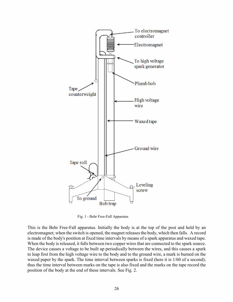
Fig. 1 - Behr Free-Fall Apparatus

This is the Behr Free-Fall apparatus. Initially the body is at the top of the post and held by anelectromagnet; when the switch is opened, the magnet releases the body, which then falls. A recordis made of the body's position at fixed time intervals by means of a spark apparatus and waxed tape. When the body is released, it falls between two copper wires that are connected to the spark source.The device causes a voltage to be built up periodically between the wires, and this causes a sparkto leap first from the high voltage wire to the body and to the ground wire, a mark is burned on thewaxed paper by the spark. The time interval between sparks is fixed (here it is 1/60 of a second);thus the time interval between marks on the tape is also fixed and the marks on the tape record theposition of the body at the end of these intervals. See Fig. 2.

26

Fig. 2 - Sample tape and demonstration of falling bob

When you obtain a tape, inspect it and draw a small circle around each mark made by the spark apparatus to help with the identification of the position marks. You will obtain the acceleration ofgravity, g, by two methods. The difference in the methods is in the analysis of the data on the tape.

Method I:

1. Choose a starting point and from that point on, label your points, 1, 2, 3 . . . n.

2. Obtain the distance ÄS in cm between two successive points. For example, assume the distance between points 3 and 4 is: 4.52cm. Thus, ÄS=4.52cm.

3. Obtain the average velocity over each of these distances.

Note that the time interval Ät between two successive points is s.

4. Obtain the successive changes in average velocities ÄV then use these changes to compute theacceleration for each particular change.

27

Fig. 3 - Sample graph of V vs t

5. Tabulate your data as follows:

nÄS

[cm]

t= n Ät

[s]

[cm/s]

ÄV

[cm/s] [cm/s2]

1 1/60

2 2/60

3 3/60

.

.

.

.

.

.

n n/60

Note:

6. Obtain g by taking the average of the values of a on the 6th column of your table. State g and the% difference of your result.

Method II:

1. Plot a graph of velocity V versus time t; the independent variable should be plotted on theabscissa and the dependent variable along the ordinate.

2. Determine g from the slope of the graph, the units should be cm/s2.

28

3. Convert your value of g from cm/s2 to m/s2. Compute the % difference.

4. Estimate errors of g and compare your results with the theoretical value of g = 9.80 m/s2.

Questions:

1. Does any part of the experiment show that all bodies fall with constant acceleration?

2. What is the significance of the constants in the equation relating V and t you plotted?

3. In relation to your experimental data:3a. Why doesn't the graph of V versus t (Method 2) go through the origin?3b. At what time did the body start to fall?3c. With what velocity did the body start to fall?3d. Can you determine the position of the bob when it started to fall?

4. What physical significance does negative time have in your equation relating V and t?

5. In terms of a V vs t graph:5a. What would be the effect on your graph if there is a change in the time interval between

sparks?5b. What would be the effect if we had used a body with twice the original mass of the body to

do the experiment?

6. In regards to the two methods used in this experiment:6a. What are the advantages in terms of analysis by Method 2 as compared to Method 1?6b. Which method do you feel is the “best?” 6c. What are the advantages (or disadvantages) in Method 1 over that Method 2? Support your

answer.

29

30

Fig. 1 - Set-up

HORIZONTAL PROJECTILE MOTION

Apparatus:

S One long steel poleS One short steel poleS One table clampS One small V-groove clampS One right angle clampS Launching trackS Small steel ballS Level and plumb bobS Carbon paperS 11" x 17" white paper and masking tapeS Meter stick and ruler

Introduction:

For a projectile near the surface of the earth the position of a particle in a trajectory is broken up intoits X and Y coordinates in the plane of the trajectory. Thus, we examine the most general vectorequation for displacement.

Eq. 1

from which we deduce two equations for the "X" displacement and the "Y" displacement.

Eq. 2

Eq. 3

In the case of a projectile fired horizontally (e.g., ball rolls off a table) there is no initial velocity inthe Y-direction. Hence, Voy = 0 in above equations and we are left with Eq. 4

Eq. 5

These are the position equations applicable to horizontal motion. They give the "X" distance andthe "Y" distance from a starting point at time "t.” You are now to determine what the initialhorizontal velocity Vo in Eq.4 of a ball rolling off a launching track by making measurements of the"X" and "Y" displacements and then studying various aspects of its trajectory.

31

Fig. 2 - Horizontal Projectile

Procedure:1. Let a ball roll off the launching track (in a high position) from a known position on the incline

and fall on a sheet of carbon paper placed atop a piece of plain paper. Measure the total distancedisplaced in the X direction from X=0 (use a plumb line at the point of launch to find X=0). Measure the total Y displacement; the distance from the launching point to the table. Since thetime to cover the total X and Y displacements is the same, use Eq.(4) and Eq.(5) to calculate Vo,the initial horizontal velocity with your measured values.

2. Repeat the above procedure identically nine (9) more times and obtain an average value for thehorizontal velocity as well as an error from the average making sure you always start the rollfrom the same point on the incline.

3. Obtain seven other X and Y points of the trajectory by lowering the launching track. Take anaverage of three rolls to determine X for each value of Y. Plot all eight (8) points on a graph ofX versus Y. This should show the trajectory of the ball after it leaves the track.

4. Use equations 4 and 5 to eliminate the variable t to obtain equation y=f(x). This is themathematical model of the trajectory. Plot it on the same graph of Procedure 3 provided you usethe value of V0 you obtained earlier.

5. Estimate errors of the trajectory.

Questions:

1. Which graph is more precise?

2. How long was the ball in the air from the highest position of the launch? (Use Eq. 4 and 5 andyour data).

3. If you change the initial velocity do you expect the trajectory to change? (Use the equation toprove this).

4. Even if you roll the ball from the same spot on the incline you get slightly different initial velocities. Why?

32

33

EQUILIBRIUM OF A RIGID BODY Apparatus

:

- Meter stick - One knife-edge meter stick clamp without clips - Two knife-edge meter stick clamps with clips - Two 50gr hangers - Slotted weights - Meter stick support stand - Large friction box - Electronic balance Introduction

:

If a rigid body is in equilibrium, then the vector sum of the external forces acting on the body yields a zero resultant and the sum of the torques of the external forces about any arbitrary axis is also equal to zero. Stated in equation form:

𝛴𝐹 = 0 𝛴𝜏 = 0 𝐸𝑞. 1 In this lab work force is defined as the mass m times gravitational acceleration g:

𝐹 = 𝑚𝑔 𝐸𝑞. 2 where m is in kg and g in m/s2 therefore, force F is in newtons N. Torque is a measure of how effective a given force is at twisting or turning the object it is applied to. Torque is defined as the force F times the moment arm or lever arm r of the force with respect to a selected pivot point x. In other words r is the distance from the pivot to the point where a force is applied. If the force is perpendicular to r, then

𝜏 = 𝐹𝑟 𝐸𝑞. 3 The unit of torque is Newton-meter, N∙m. The sign for torque is defined as positive (+) when rotating in counter-clockwise direction and negative (-) when rotating in a clockwise direction. In this experiment a meter stick is used as a rigid body to illustrate the application of the equations of equilibrium. The torque equation will be verified for a balanced system of two masses. The torque equation will also be applied to determine the mass of the meter stick and compare to the known value. For this experiment it is not only important to familiarize yourself with the equations, but also with sketching free-body diagrams (FBD). Next are examples of balanced systems and application of the torque equation. The equations must be solved as a pre-lab exercise.

34

1. Meter stick in equilibrium, fulcrum at its center and masses on opposite sides of the balance point.

Fig. 1 – Balanced system with two masses and corresponding FBD

Since Στ=0 and knowing that τ=Fr we can develop the equation of equilibrium based on the FBD taking into account the signs of the torques. r is the distance from the pivot point to the point where the force is applied. In the case above we have F1 acting at point x1 that will cause a counterclockwise rotation with respect to the pivot point xo therefore, torque is positive. F2 is acting at point x2 and will cause a clockwise rotation with respect to the pivot point xo thus making the torque negative. Therefore,

𝛴𝜏 = 𝜏1 − 𝜏2 = 0 𝐸𝑞. 4 or

𝜏1 = 𝜏2 𝐸𝑞. 5 Rewriting in terms of F and r:

(𝐹1)(𝑟1) = (𝐹2)(𝑟2) 𝐸𝑞. 6 where F=mg

(𝑚1𝑔)(𝑟1) = (𝑚2𝑔)(𝑟2) 𝐸𝑞. 7 Then:

(𝑚1𝑔)(𝑥𝑜 − 𝑥1) = (𝑚2𝑔)(𝑥2 − 𝑥𝑜) 𝐸𝑞. 8 Let us assume that in this system we have: m1=0.110 kg (includes the mass of the clamp) suspended at x1=0.223 m, m2=0.081 kg (includes the mass of the clamp) suspended at x2=0.890 m and the pivot point is located at xo=0.506 m. Substitute the given values along with g=9.8 m/s2 into the equation above. How does 𝜏1 compare to 𝜏2?

Fulcrum

x1 xo x2

m1 m2

x1 xo x2

m1*g

r1 r2

N

M*g m2*g

Fulcrum

x1 xo x2

m1 m2

x1 xo x2

m1*g

r1 r2

N

M*g m2*g

35

Note that the location x is read from the inside edge of the meter stick clamp. In the case of Fig. 2 the location is 41.5 cm or 0.415 m.

2. Balanced meter stick with one mass. Determining the mass of the meter stick.

Fulcrum

x'o

m1

xo x1

CG

xo x'o x2

m1*g

ro r1

N

M*gms*g

New pivot point

Fig. 3 - System with one mass and balanced at new pivot point plus corresponding FBD

Fig. 3 shows one mass suspended on the right side of the meter stick and a new pivot point was determined in order for the system to be in equilibrium. The torque equation will be applied with respect to the new pivot point 𝑥𝑜′ and use it to calculate the experimental mass of the meter stick.

𝛴𝜏 = 𝜏𝑜 − 𝜏1 = 0 𝐸𝑞. 9 Rewriting:

𝜏𝑜 = 𝜏1 𝐸𝑞. 10

(𝑀𝑔)(𝑟𝑜) = (𝑚1𝑔)(𝑟1) 𝐸𝑞. 11

(𝑀𝑔)(𝑥𝑜′ − 𝑥𝑜) = (𝑚2𝑔)(𝑥1 − 𝑥𝑜′ ) 𝐸𝑞. 12 Solving for M:

𝑀 =(𝑚1𝑔)(𝑥1 − 𝑥𝑜′ )

(𝑔)(𝑥𝑜′ − 𝑥𝑜)=

(𝑚1)(𝑥1 − 𝑥𝑜′ )(𝑥𝑜′ − 𝑥𝑜)

𝐸𝑞. 13

Fig. 2 – Meter stick clamp

36

In this system we have: m1=0.061 kg (includes the mass of the clamp) suspended at x1=0.792 m, M acting at the original pivot point xo=0.506 m, New pivot point 𝑥𝑜′ is located at 𝑥𝑜′ = 0.627 m. The known mass of the meter stick 0.0842 kg. Calculate the experimental mass and compare to the known value by means of the percent difference formula. 3. Balanced meter stick with two masses (one known and one unknown) at opposite sides

of the fulcrum:

Fulcrum

xu xo x1

mum1

xu xo x2

mu*g

ru r1

N

m1*gM*g

Fig. 3 - Balanced system with one unknown mass and a known mass and corresponding FBD

Therefore, 𝛴𝜏 = 𝜏𝑢 − 𝜏1 = 0

or 𝜏𝑢 = 𝜏1

Rewriting in terms of F and r: (𝐹𝑢)(𝑟𝑢) = (𝐹1)(𝑟1)

where F=mg

(𝑚𝑢𝑔)(𝑟𝑢) = (𝑚1𝑔)(𝑟1) Then:

(𝑚𝑢𝑔)(𝑥𝑜 − 𝑥𝑢) = (𝑚1𝑔)(𝑥1 − 𝑥𝑜)

𝑚𝑢 =(𝑚1𝑔)(𝑥1 − 𝑥𝑜)

(𝑔)(𝑥𝑜 − 𝑥𝑢)=

(𝑚1)(𝑥1 − 𝑥𝑜)(𝑥𝑜 − 𝑥𝑢)

Do not forget that mu = mass of the unknown object + mass of the clamp Let us assume that in this system we have: m1=0.152 kg (includes the mass of the clamp) suspended at x1=0.90 m, Mass of the clamp that holds the object of unknown mass is 0.017 kg, mu is located at xu=0.289 m

37

the pivot point is located at xo=0.499 m and Mass of the unknown object found by weighing it is 0.272 kg Use the torque equation to calculate the mass of the unknown object. How does the calculated mass compare to the value determined by the electronic scale? Experiment Procedure

:

Part I. Balancing the meter stick without masses to determine the pivot point

:

1. Weigh the meter stick by itself on the electronic balance and record its mass. 2. Determine and record the mass of the clamps with clips. 3. Put the meter stick through the clamp that has no clips (the clamp should be upside down so

that the lock screw is on the bottom). Slide the clamp to a point near the center of the meter stick. Position the clamped meter stick on the support stand. Gently slide the meter stick through the clamp till the rigid body is in equilibrium. Once it is, lock the clamp in place (Fig. 4). Record the location of the balance point by reading from the inside edge of the knife-edge clamp.

Fulcrum

xo

CG

Fig. 4 – Balanced meter stick

Part II. Balancing the rigid body with two masses on opposite sides of the fulcrum

:

1. Secure one clamp at the 5 cm mark (left of the fulcrum) and suspend a mass of 50 g. 2. Place the second clamp at an arbitrary point to the right of the fulcrum. 3. Hang 100 g from the second clamp. 4. Adjust the position of m2 till the system is in equilibrium. 5. Record the masses and positions. Do not forget to include the mass of the clamps to each

mass. 6. Draw the corresponding FBD and write the torque equation about the pivot point. 7. Compare and express the percent difference between the torques. 8. Slide m1 to the 15 cm position and adjust the location of m2 so that the system is equilibrium. Part III. Obtaining the mass of the meter stick by method of torques

:

1. Balance the meter stick by itself. 2. Position one clamp at the 5 cm mark and suspend 100 g from it. 3. Find a new pivot point that will bring the system to equilibrium. Record the location. 4. Using the torque equation calculate the mass of the meter stick. 5. Compare the obtained value with the value you found when weighing the meter stick.

38

Part IV. Balancing the rigid body with one known mass and one unknown mass

:

1. Place one clamp at the 20 cm mark and suspend 100 g from it. 2. Place the second clamp at an arbitrary position on the opposite side of the fulcrum and hang

the unknown object from it. The combination of the clamp and the unknown object becomes mu.

3. Adjust the position of mu till the system is in equilibrium. 4. Use the torque equation to solve for the unknown mass. Subtract the mass of the clamp from

the calculated value. 5. Weigh the unknown object on the electronic balance and compare to the calculated value.

Part V. Calculating and checking a pivot point that will balance the system with two masses located at designated points

:

1. If you have 100g suspended at the 0.05 m mark and 0.050 kg at the 0.60 m mark calculate the location of the pivot point required to balance the system.

2. Test your results on the meter stick by placing the required masses and adjusting the meter stick to find the balance point. How does it compare to the calculated value?

Questions

:

1. A meter stick is balanced at its center. If a 3 kg mass is suspended at x=0 m, where would you need to place a mass of 5 kg to have the system in equilibrium?

2. What will happen if the meter stick is not strictly horizontal? 3. Can we apply the torque balance equation if the stick is not horizontal? What must be

changed in Eq. 3, 6, 7, 8, 11, 12 and 13 in this case?

Fig. 1 - Set-up for block on a horizontal plane

Fig. 2 - Forces acting on the system

FRICTION

Apparatus:

S Friction blockS Friction boardS PulleyS 50gr hangerS Slotted weightsS StringS Electronic balanceS Meter stick or pendulum protractor

Theory:For a large class of surfaces the ratio of the (static and kinetic) frictional force, f, to the normal force,N, is approximately constant over a wide range of forces. This ratio defines, for specific surfaces,the coefficient of friction, namely:

In the static case when our applied force reaches a value such that the object instantaneously startsto move we obtain the maximum frictional force or limiting value of the frictional force fmax.

We can now obtain the coefficient of staticfriction defined as:

When the object is moving it experiences africtional force, fK which is less than thestatic. Frictional experiments tell us that wecan (analogous to the static case) define acoefficient of kinetic friction given by:

Procedure:

1. Set up the equipment as in Fig. 1.

2. Weigh the block, W1.

39

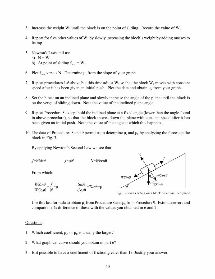
Fig. 3 -Forces acting on a block on an inclined plane

3. Increase the weight W2 until the block is on the point of sliding. Record the value of W2.

4. Repeat for five other values of W1 by slowly increasing the block’s weight by adding masses toits top.

5. Newton's Laws tell us: a) N = W1

b) At point of sliding fmax = W2

6. Plot fmax versus N. Determine ìs from the slope of your graph.

7. Repeat procedures 1-6 above but this time adjust W2 so that the block W1 moves with constantspeed after it has been given an initial push. Plot the data and obtain ìk from your graph.

8. Set the block on an inclined plane and slowly increase the angle of the plane until the block ison the verge of sliding down. Note the value of the inclined plane angle.

9. Repeat Procedure 8 except hold the inclined plane at a fixed angle (lower than the angle found

in above procedure), so that the block moves down the plane with constant speed after it hasbeen given an initial push. Note the value of the angle at which this happens.

10. The data of Procedures 8 and 9 permit us to determine ìs and ìk by analyzing the forces on theblock in Fig. 3.

By applying Newton’s Second Law we see that:

From which:

Use this last formula to obtain ìs from Procedure 8 and ìk from Procedure 9. Estimate errors andcompare the % difference of these with the values you obtained in 6 and 7.

Questions:

1. Which coefficient, ìs, or ìk is usually the larger?

2. What graphical curve should you obtain in part 6?

3. Is it possible to have a coefficient of friction greater than 1? Justify your answer.

40

41

NEWTON'S SECOND LAW (Vernier LabQuest2 - computer interfaced version)

Apparatus

:

- Vernier dynamics track - Smart-pulley system - Friction box - 50gr hanger - Slotted weights - String - Long rod - Table clamp - Electronic balance - Digital angle finder - LabQuest2 - LoggerPro software Fig. 1 – Experiment set-up for block accelerating on a horizontal plane Introduction

:

Newton's Second Law can be written in vector form as: Σ 𝐅 = ma Eq. 1

where ΣF is the vector sum of the external forces acting on a body and a is the resultant acceleration of the c.g. of the body. If F is constant, then a is constant and the equations of motion with constant acceleration apply, i.e.,

S = Vot +12

at2 Eq. 2 A. For the horizontal plane:

With N=Normal force, T=Tension in the cord and fk=Kinetic frictional force=μkN then:

Fig. 2 - Forces acting on a system with a block accelerating a long a horizontal plane

LabQuest2

AngleFinder 50g

Hanger

DynamicsTrack

Friction BoxStopper Pulley and Photogate

FrontStopper

Table Clampand Rod

m1

m2

N

fk

m1g

m2g

T

Tx

y

+a

42

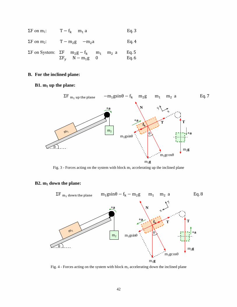
ΣF on m1: T − fk = m1 a Eq. 3 ΣF on m2: T − m2g = −m2a Eq. 4 ΣF on System: ΣF = m2g − fk = (m1 + m2)a Eq. 5 ΣFy = N − m1g = 0 Eq. 6 B. For the inclined plane:

B1. m1 up the plane:

ΣF(m1 up the plane) = −m1gsinθ − fk + m2g = (m1 + m2)a Eq. 7

m1 m2

N

fkT

+a

θ

θ

+a

m1gsinθ

m1gcosθ

m1g

+a

T

m2g

xy

Fig. 3 - Forces acting on the system with block m1 accelerating up the inclined plane

B2. m1 down the plane: ΣF(m1 down the plane) = m1gsinθ − fk − m2g = (m1 + m2)a Eq. 8

m1m2

N

fk T

+a

θ

θ

+a

m1gsinθ

m1gcosθ

m1g

+a

T

m2g

x

y

Fig. 4 - Forces acting on the system with block m1 accelerating down the inclined plane

43

The perpendicular forces acting on the system whether the block is accelerating up or down an inclined plane are:

ΣFy = N − m1gcosθ Eq. 9 Procedure

:

Preliminary set-up: 1. Set up the dynamics track in a flat position as in Fig. 1, use the digital angle finder to make

sure that the angle is 0.0o. Connect the photogate cable into one of the digital ports of the LabQuest2, turn it on and connect it to the computer.

2. Open the Physics Folder. Open the PhyExpTemplates folder, open the LoggerProTemplates folder. Open the Newton2ndLawExp file. A dialog window may pop-up requesting sensor confirmation, if that is the case click “connect.” The file is made up of 3 pages: Page 1: Exp. To collect acceleration data. Page 2: Flat. To analyze data for track in flat position and determine µk. Page 3: Incline. To analyze data for the friction box moving up and down the track at a fixed angle.

Part I: Measuring acceleration of a friction box moving along the flat track by means of the Smart-Pulley System1

1. Place 100 g inside the friction box and weigh it. Record the mass as m1 on “Page 2: Flat”. and determining µk:

2. Place slotted weights on the hanger (m2) that will cause m1 to accelerate along the plane. Test it before collecting data with the Smart-Pulley system.

3. Record the total hanging mass on Page 2 in the m2 column. 4. When ready and making sure that m2 is not swinging click the "collect" tab located

on the top toolbar and allow the block (m1) to be pulled by the hanging mass (m2). As the Smart-Pulley system collects data a Velocity vs Time graph will automatically be created. The collection will stop on its own. Before proceeding show the graph to your instructor if the graph looks odd repeat the procedure for same masses otherwise increase or decrease m2 to achieve a better acceleration.

5. When the graph is complete select an area of the graph where acceleration is constant and obtain the slope of the graph by clicking on “R” Record it as acceleration "a" in Page 2. See Fig. 5 for a sample graph.

6. Change m1 in steps of 50 g and determine m2 that will cause m1 to accelerate along the plane. Collect the acceleration. Note: Some may prefer to keep m1 and m2 constant and repeat procedure 5 times to have a total of 6 accelerations.

7. Calculate the Normal, Tension, Kinetic Frictional forces and µk. 8. Compute the average µk. (Another method to obtain µk is by plotting Kinetic Frictional

Force vs Normal Force and determining the slope just as it was done for the Friction experiment.)

1See Appendix 3 for description of the Smart-Pulley System.

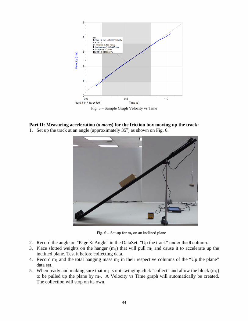
44

Fig. 5 – Sample Graph Velocity vs Time Part II: Measuring acceleration (a meas) for the friction box moving up the track: 1. Set up the track at an angle (approximately 35o) as shown on Fig. 6.

Fig. 6 – Set-up for m1 on an inclined plane

2. Record the angle on "Page 3: Angle” in the DataSet: "Up the track” under the θ column. 3. Place slotted weights on the hanger (m2) that will pull m1 and cause it to accelerate up the

inclined plane. Test it before collecting data. 4. Record m1 and the total hanging mass m2 in their respective columns of the “Up the plane”

data set. 5. When ready and making sure that m2 is not swinging click "collect" and allow the block (m1)

to be pulled up the plane by m2. A Velocity vs Time graph will automatically be created. The collection will stop on its own.

45

6. When the graph is complete select an area of the graph where acceleration is constant and obtain the slope of the graph. Record it as acceleration "ameas" in Page 3.

7. Increase m1 and repeat steps 3 to 6. 8. Calculate the acceleration using Eq. 7. 9. Compare the calculated acceleration to the measured acceleration. Express the % difference.

Part III: Measuring the acceleration (a meas) for a friction box moving down the track: 1. Keep the track at the same angle as in the previous procedure. Record it in the DataSet:

"Down the track" under the θ column. 2. Adjust m2 so that m1 accelerates down the inclined plane. Test it before collecting data. 3. Record m1 and the total hanging mass m2 in their respective columns of the “Down the

plane” data set. 4. When ready and making sure that m2 is not swinging click "collect" and allow m1 to

accelerate down the plane. A Velocity vs Time graph will automatically be created. The collection will stop on its own.

5. When the graph is complete select an area of the graph where acceleration is constant and obtain the slope of the graph. Record it as acceleration "ameas" in the respective data set in Page 3.

6. Increase m1 and repeat steps 3 to 6. 7. Calculate the acceleration using Eq. 8. 8. Compare the calculated acceleration to the measured acceleration. Express the % difference.

Printing the Data Tables: 1. Go to the File menu. Select “Page Set-up…” Select “Landscape.” Click OK. 2. Click on the print icon or select “Print” from the File menu. 3. Select the box “Print Footer.” This will allow you and your laboratory partner(s) to enter

your names. Click “OK.” 4. Enter the pages you wish to print. If you wish to print just the data tables from Page 2 and

Page 3 select “Print Data Table” from the File menu and follow steps 2 and 3.

46

47

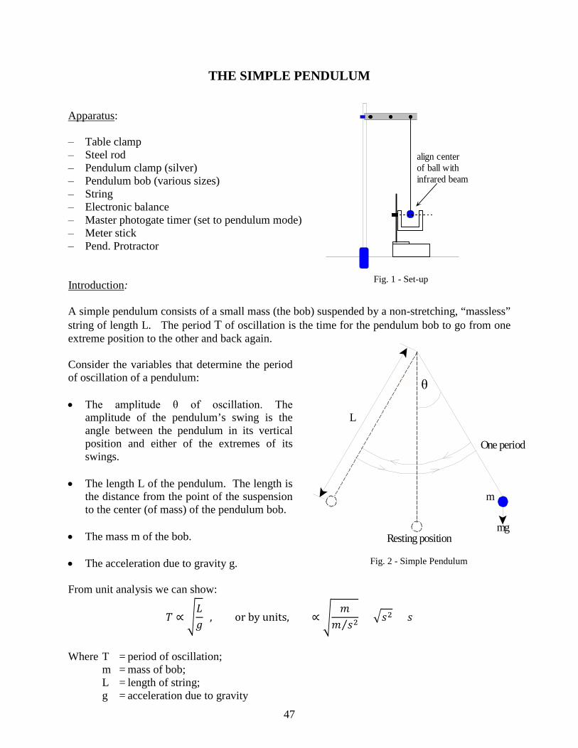
THE SIMPLE PENDULUM Apparatus

:

‒ Table clamp ‒ Steel rod ‒ Pendulum clamp (silver) ‒ Pendulum bob (various sizes) ‒ String ‒ Electronic balance ‒ Master photogate timer (set to pendulum mode) ‒ Meter stick ‒ Pend. Protractor Introduction

:

A simple pendulum consists of a small mass (the bob) suspended by a non-stretching, “massless” string of length L. The period T of oscillation is the time for the pendulum bob to go from one extreme position to the other and back again. Consider the variables that determine the period of oscillation of a pendulum: • The amplitude θ of oscillation. The

amplitude of the pendulum’s swing is the angle between the pendulum in its vertical position and either of the extremes of its swings.

• The length L of the pendulum. The length is

the distance from the point of the suspension to the center (of mass) of the pendulum bob.

• The mass m of the bob. • The acceleration due to gravity g. From unit analysis we can show:

𝑇 ∝ �𝐿𝑔

, or by units, ∝ �𝑚

𝑚 𝑠2⁄ = �𝑠2 = 𝑠

Where T = period of oscillation; m = mass of bob; L = length of string; g = acceleration due to gravity

align centerof ball withinfrared beam

Fig. 1 - Set-up

L

θ

m

mgResting position

One period

Fig. 2 - Simple Pendulum

48

Since an oscillation is described mathematically by cos ωt and knowing that ω=2πf where f = 1/T we then have:

𝑇 =2𝜋𝜔

Eq. 1 Equation 1 can be re-writen as:

𝑇 = 2𝜋�𝐿𝑔

Eq. 2

Procedure

:

Make the following measurements: 1. Turn on the photogate and set it to pendulum mode. In addition, make sure the memory

switch on as well. Set-up the pendulum so that when it is in resting position it blocks the photogate as shown on Fig. 1.

2. Period as a function of amplitude (plot T vs. θ). Perform this procedure for amplitudes of

5° to 30° in steps of 5°. The length and mass will remain constant. At each given angle allow the pendulum to swing through the photogate, be careful not to strike the photogate with the pendulum. Record the period displayed on the photogate that corresponds to the amplitude.

3. Period as a function of length (plot T vs. L). Use a small angle such as 10°. Change the

length 6 times. Each time a new length L is set, the length must be measured from the center of the bob to the pivot point. The amplitude and the mass will remain constant. Allow the pendulum to swing through the photogate and record the period displayed on the photogate. Fit the data to Eq. 2. How does the obtained “g” value from the fit compare to the known value of “g”?

Note: An alternate method for this procedure is to plot T2 vs L and use the best linear fit to determine the slope. Then use the slope to obtain g and compare to the known value. The linear fit would be of the form: 𝑇2 = 4𝜋

𝑔𝐿.

4. Period as a function of mass (plot T vs. m). Use a small angle such as 10°. Use 4

different masses but keep amplitude and length constant. For each mass record the period as displayed on the photogate.

Questions

:

1. For the simple pendulum where is the maximum for: displacement, velocity and acceleration?

2. Would the period increase or decrease if the experiments were held on : a) the top of a high mountain? b) the moon? c) on Jupiter?

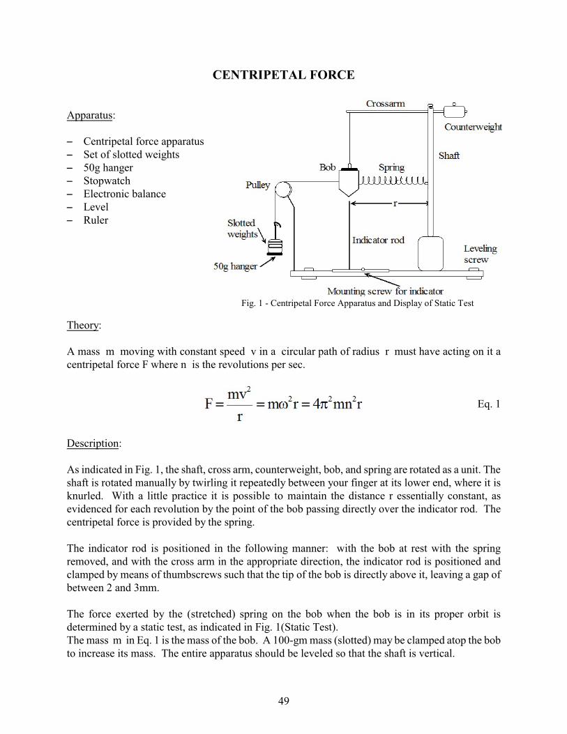
Fig. 1 - Centripetal Force Apparatus and Display of Static Test

CENTRIPETAL FORCE

Apparatus:

S Centripetal force apparatusS Set of slotted weightsS 50g hangerS StopwatchS Electronic balanceS Level S Ruler

Theory:

A mass m moving with constant speed v in a circular path of radius r must have acting on it acentripetal force F where n is the revolutions per sec.

Eq. 1

Description:

As indicated in Fig. 1, the shaft, cross arm, counterweight, bob, and spring are rotated as a unit. Theshaft is rotated manually by twirling it repeatedly between your finger at its lower end, where it isknurled. With a little practice it is possible to maintain the distance r essentially constant, asevidenced for each revolution by the point of the bob passing directly over the indicator rod. Thecentripetal force is provided by the spring.

The indicator rod is positioned in the following manner: with the bob at rest with the springremoved, and with the cross arm in the appropriate direction, the indicator rod is positioned andclamped by means of thumbscrews such that the tip of the bob is directly above it, leaving a gap ofbetween 2 and 3mm.

The force exerted by the (stretched) spring on the bob when the bob is in its proper orbit isdetermined by a static test, as indicated in Fig. 1(Static Test).The mass m in Eq. 1 is the mass of the bob. A 100-gm mass (slotted) may be clamped atop the bobto increase its mass. The entire apparatus should be leveled so that the shaft is vertical.

49

Fig. 2 - Centripetal Force Apparatus Rotating

Procedure:

Devise a method for determining whether the shaft is vertical, and make any necessary adjustmentsof the three leveling screws.

The detailed procedure for checking Eq. 1experimentally will be left to the student. At least three values of r should be used,with two values of m for each r. Amethod for measuring r should be thoughtout, for which purpose the vernier calipermay be useful. The value of n should bedetermined by timing 50 revolutions ofthe bob, and then repeating the timing foran additional 50 revolutions. If the timesfor 50 revolutions disagree by more thanone-half second, either a blunder incounting revolutions has been made, orthe point of the bob has not beenmaintained consistently in its propercircular path.

Results and Questions:

1. Exactly from where to where is r measured? Describe how you measured r.

2. Tabulate your experimental results. 3. Tabulate your calculated results for n, F from static tests, and F from Eq. 1, and the % difference

between the F's, using the static F as standard. Estimate % error.

4. Describe how to test whether the shaft is vertical without the use of a level. Why should it beexactly vertical?

5. Why is the mass of the spring not included in m?

50

51

WORK AND KINETIC ENERGY

Apparatus:

Linear Air-Track with variable output air supply and hose

Two master photogate timers

Two gliders and an air-track kit

Electronic balance

Theory:

Work and kinetic energy are related as:

Work = Change of Kinetic Energy

If the total work done by all the forces on the system is zero, the total kinetic energy remains

constant. Consider a system of two masses, m1 and m2 moving at velocities, v1i and v2i, about to

undergo a collision. Before the collision the kinetic energy is:

𝐾𝐸𝑖 =1

2𝑚1𝑣1𝑖

2 +1

2𝑚2𝑣2𝑖

2

After the collision the two bodies move off with velocities v1f and v2f respectively. Thus, the

kinetic energy after the collision is:

𝐾𝐸𝑓 =1

2𝑚1𝑣1𝑓

2 +1

2𝑚2𝑣2𝑓

2

Pre-lab Exercise: Before the day of the experiment run the simulation below to get a better

understanding of how the experiment will work. Perform the simulation for the conditions as

listed on page 52 (note, if you want a cart to move to the left, you must make its velocity

negative): http://www.mrwaynesclass.com/teacher/Impulse/SimFriction/home.html

Procedure:

1. Setup the air track and photogates as shown in Fig.1, using bumpers on the gliders to provide

an elastic collision. Carefully level the track.

Fig. 1 – Air-Track Set-up

Photogate 1 Photogate 2

m1 m2

52

2. Measure m1 and m2, the masses of the two gliders (include the flags and bumpers) to be used

in the collision. Record your results in tabular form. Start with equal masses then use

attachments to change the masses as required in Procedure 6 below.

3. Record the length of the flags on the gliders as 0.1m each.

4. Set both Photogate Timers to GATE mode, and press RESET buttons. Make sure the

memory switch is on.

5. Estimate the % error in time by letting a glider go through the two photogates. Calculate the

% error in the time measurement.

6. The experiment will be performed for the following configurations:

1. m1 = m2 v1i ≠ 0 v2i = 0

2. m1 > m2 v1i ≠ 0 v2i = 0

3. m1 < m2 v1i ≠ 0 v2i = 0

4. m1 > m2 v1i = 0 v2i = 0 ( explosion )

5. m1 > m2 v1i ≠ 0 v2i ≠ 0

6. m1 > m2 v1i ≠ 0 v2i = 0 ( coupled )

Note, when increasing masses on a glider it must be done symmetrically.

For each configuration record four time measurements as follows:

t1i = the time that glider1 blocks photogate1 before the collision.

t2i = the time that glider2 blocks photogate2 before the collision.

(In cases where v2i = 0 there is no t2i since glider2 begins at rest.)

t1f = the time that glider1 blocks photogate1 after the collision.

t2f = the time that glider2 blocks photogate2 after the collision.

IMPORTANT: The collision must occur after glider1 has passed through photogate1 and, after

the collision, the gliders must be fully separated before either glider interrupts a photogate.

NOTE: Use the memory function in the ME-9215 Photogate Timer, to store the initial times

while the final times are being measured. The numbers on the screen reflect the first time the

glider crossed the photogate. When you flip the memory switch you get a second reading which

represents the total time a glider traveled through a photogate forth and back (after collision).

Subtract the first number from the second to obtain the final time, tf .

Calculations and Questions:

For each case:

1. Calculate the Initial Kinetic Energy, KEi, and the error in KEi. Percent error in the Kinetic

Energy = (2)*( % error in time)

2. Calculate Final Kinetic Energy, KEf and the error in Kef.

53

CONSERVATION OF MOMENTUM

Apparatus:

Linear Air-Track with variable output air supply and hose

Two master photogate timers

Two gliders

Air-Track kit

Electronic balance

Theory:

When objects collide, whether locomotives, shopping carts, or your foot and the sidewalk, the

results can be complicated. Yet even in the most chaotic of collisions, as long as there are no

external forces acting on the colliding objects, one principle always holds and gives up an

excellent tool for understanding the dynamics of the collision. That principle is called the

conservation of momentum. 𝑝𝐼 = 𝑝𝑓

where 𝑝𝑖 = 𝑚1𝑣1𝑖 + 𝑚2𝑣2𝑖 and 𝑝𝑓 = 𝑚1𝑣1𝑓 + 𝑚2𝑣2𝑓

For a two-object collision, momentum conservation is easily stated mathematically by the

equation: where m1 and m2 are the masses of the two objects, v1i and v2i are the initial velocities

of the objects (before the collision), v1f and v2f are the final velocities of the objects, and pi and pf

are the combined momentums of the objects, before and after the collision. In this experiment,

you will verify the conservation of momentum in a collision of two air track gliders.

Pre-lab Exercise: Before the day of the experiment run the simulation below to get a better

understanding of how the experiment will work. Perform the simulation for the conditions as

listed on page 54 (note, if you want a cart to move to the left, you must make its velocity

negative): http://www.mrwaynesclass.com/teacher/Impulse/SimFriction/home.html

Procedure:

1. Setup the air track and photogates as shown in Fig.1, using bumpers on the gliders to provide

an elastic collision. Carefully level the track.

Fig. 1 – Air-Track Set-up

Photogate 1 Photogate 2

m1 m2

54

2. Record the length of the flags on the gliders as 0.1m each.

3. Set both Photogate Timers to GATE mode, and press RESET buttons.

4. The experiment will be performed for the following configurations where each glider will

have a rubber band bumper except for configuration 4.5:

4.1. m1 = m2 v1i ≠ 0 v2i = 0

4.2. m1 > m2 v1i ≠ 0 v2i = 0

4.3. m1 < m2 v1i ≠ 0 v2i = 0

4.4. m1 > m2 v1i ≠ 0 v2i ≠ 0

4.5. m1 > m2 v1i ≠ 0 v2i = 0 ( coupled )

The last configuration is an example of non-elastic collision in which two gliders, instead of

bouncing off each other, stick together so that they move off with identical final velocities.

Replace the rubber bumpers with the wax and needle attachments.

5. Measure m1 and m2, the masses of the two gliders (include the flags and bumpers) to be used

in the collision. Record your results in tabular form.

Note, when increasing masses on a glider it must be done symmetrically.

6. Four time measurements will be obtained for each configuration

t1i = the time that glider1 blocks photogate1 before the collision.

t2i = the time that glider2 blocks photogate2 before the collision.

(In cases where v2i = 0 there is no t2i since glider2 begins at rest.)

t1f = the time that glider1 blocks photogate1 after the collision.

t2f = the time that glider2 blocks photogate2 after the collision.

IMPORTANT: The collision must occur after glider1 has passed through photogate1 and, after

the collision, the gliders must be fully separated before either glider interrupts a photogate. Use

the memory function to store the initial times while the final times are being measured.

Data and Calculations:

1. For each time that you measured, calculate the corresponding glider velocity (v=L/t) where

the velocity is positive when the glider moves to the right and negative when it moves to the

left.

2. Use your measured values to calculate pi and pf, the combined momentum of the gliders

before and after the collision.

3. Estimate error of pi and pf and conclude if pi=pf within these errors.

Questions:

1. Was momentum conserved in each of your collisions? If not, try to explain any

discrepancies.

2. Suppose the air track was tilted during the experiment. Would momentum be conserved in

the collision? Why or why not?

55

ROTATIONAL MOTION AND MOMENT OF INERTIA (Vernier LabQuest2 - computer interfaced version)

Apparatus- Vernier dynamics track

:

- Adjustable end stop - Motion detector - Clamp and rod support - Digital angle finder - Solid cylinder - Hollow cylinder - Solid sphere Fig. 1 – Experiment Set-up - Hollow sphere - LabQuest2 interface and LoggerPro software

TheoryThe motion of a rigid body is the combination of translation and rotation. The rotational inertia, I, of a body rotating about a fixed axis measures the resistance of the body to angular acceleration when a torque is applied. The torque, τ, is the product of force times lever arm (perpendicular distance from the line of action of the force to the axis of rotation). The angular acceleration, α, is the rate of change of angular velocity. The variation of the moment of inertia as a function of mass distribution or shape of the object will be investigated.

:

Table I

Rotational Inertia, I, about the axis of symmetry Solid Cylinder Hollow Cylinder Solid Sphere Hollow Sphere

12𝑚𝑅2 𝑚𝑅2

25𝑚𝑅2

23𝑚𝑅2

The moment of inertia is to rotational motion what the mass of an object is to translational motion. This analogy can be illustrated as follows1

:

Table II Translational Motion

F = ma Analogy Rotational Motion τ = Iα

F driving force τ

m resistance to changes in velocities I

a acceleration or response to changes in velocities α

1Adapted from PHY 211 - Lab 6 - Univeristy of Illinois up to Eq. 3

Dynamics trackRolling object Motion sensor

Endstopper

Rod andclamp

56

Consider an object rolling down an inclined plane having an angle θ:

Fig. 2 – Object rolling down an inclined plane

The sum of the forces yielding the object’s translational acceleration along the ramp is given by:

𝛴𝐹 = 𝑚𝑔 𝑠𝑖𝑛𝜃 − 𝑓 = 𝑚𝑎 Eq. 1

The sum of the torques providing the object’s acceleration α about its center can be written:

𝛴𝜏 = 𝑓𝑅 = 𝐼𝛼 Eq. 2 Because the objects roll without slipping, one also has the following relationship between the translational and rotational accelerations:

𝑎 = 𝑅𝛼 Eq. 3 take:

𝐼 = 𝑘 𝑚 𝑅2 Eq. 4 where k represents the inertial constant. The value of k will depend on the shape of the object and can have a value from 0 to 1. Substituting equations 1 to 3 into Eq. 4 and solving for k we obtain:

𝑘 =𝑔𝑠𝑖𝑛𝜃𝑎

− 1 Eq. 5 Fig. 3 depicts four objects on the verge of rolling down the inclined plane which object do you think will reach the finish line first? Remember that because of their shape each object has a different inertial constant k value and therefore different moments of inertia I.

Fig. 3 – Objects on a inclined plane Click on the link2

https://upload.wikimedia.org/wikipedia/commons/4/41/Rolling_Racers_-_Moment_of_inertia.ogv to see the animation and confirm your prediction:

2 Created by Lucas Barbosa and OGG Theora Video

θ

R

f

F=mg

mg sin θθ

mg cos θ

57

Preliminary set-up

:

1. Set up the plane at small angle as in Fig. 1. Place the digital angle finder atop the ramp and gently adjust the height so that the angle reads 6o.

2. Slide the switch on the motion detector3

3. Turn on the LabQuest2 interface and connect it to the computer.

to "cart" mode. Connect the motion detector to one of the digital ports of the LabQuest2 unit.

4. Open the Physics Folder. Open the PhyExpTemplates folder, open the LoggerProTemplates folder. Open the RotationalMotionMomentInertiaExp file. The file is made up of 2 pages, Page 1: To collect data, Page 2: To record and analyze data.

Procedure

:

1. Select one of the objects: hollow cylinder, hollow sphere, solid cylinder or solid sphere. 2. Record the angle of the incline on Page 2 of the experiment template under the θ column

within the data set that corresponds to the selected object. 3. Position the object on the ramp at a distance 15cm to 20cm in front of the motion detector. 4. Go back to Page 1 of the template. Click "collect," once the motion detector starts making

clicking sounds allow the object to roll down the ramp. 5. From the Velocity vs Time graph select and area that shows the object rolling down the ramp

with constant acceleration. Click on "R" to obtain the slope which represents the acceleration.

6. Record the slope of the line on Page 2 under the column labeled a. 7. Perform three more runs for the same object and obtain the corresponding slopes. 8. Repeat steps 3 to 7 for other objects recording the data in the corresponding data sets.

Calculations and Exercises

:

For each object: 1. Calculate the corresponding k value for each object using Eq. 5. 2. Evaluate the % error in k. 3. Find % differences in k for all shapes studied. 4. Make the conclusion about how close (or how far) your measured k values are to (from) the

given ones as listed on Table 1.

3 For information on how the motion detector works please see Appendix 3.

58

SUPPLEMENTARYEXPERIMENTS

59

60

61

DENSITY AND ARCHIMEDES' PRINCIPLE

Apparatus:

‒ Electronic balance

‒ Hook stand and beaker base

‒ 600ml plastic beaker

‒ Aluminum cylinder with hook

‒ Brass pendulum bob (2.54cm)

‒ String

‒ 500ml graduated cylinder with water

‒ Ruler or Vernier caliper

Introduction:

Archimedes's principle states that a body immersed in a fluid is buoyed up by a

force equal to the weight of the displaced fluid (Fig. 2).

Imagine now that a body is suspended in water as shown in Fig. 3b. The

effective weight of the body (Weff) as measured by the masses on the scale is

given by:

𝑊𝑒𝑓𝑓 = 𝑀′𝑔 Eq. 1

but the effective weight is equal to the weight of the object minus the buoyant

force.

𝑊𝑒𝑓𝑓 = 𝑊 − 𝐵 Eq. 2

Fig. 3 - (a) Object in air (b) Object submerged in water

Buoyant

Force

Weight

of Object

Fluid

Object

L

Li

M

Empty vessel

L

M'

Partially filled vessel

(a) (b)

Fig. 1 - Set-up

62

By Archimedes's principle:

𝐵 = 𝜌𝐻2𝑂𝑉𝑖𝑔 Eq. 3

Substituting Eq. 3 into Eq. 2:

𝑊𝑒𝑓𝑓 = 𝑊 − 𝜌𝐻2𝑂𝑉𝑖𝑔 Eq. 4

𝑊𝑒𝑓𝑓 = 𝑊 − 𝜌𝐻2𝑂𝑉𝑖𝑔𝑊

𝑊 Eq. 5

𝑀′𝑔 = 𝑚𝑔 − 𝜌𝐻2𝑂𝑉𝑖𝑔𝑀𝑔

𝜌𝑉𝑔 Eq. 6

𝑀′ = 𝑀 −𝑀𝜌𝐻2𝑂

𝜌𝐿

𝑉𝑖

𝑉 Eq. 7

If the cross sectional area is constant, Eq. 7 reduces to:

𝑀′ = −𝑀𝜌𝐻2𝑂

𝜌𝐿𝐿𝑖 + 𝑀 Eq. 8

Where:

M’ = mass of the cylinder when it is partially submerged in water.

ρH2O = density of water.

ρ = density of the object

L = total length of the object

Li = length of the part of the cylinder that is submerged in water

M = mass of the object

Note that Eq. 8 is of the form:

𝑦 = 𝑚𝑥 + 𝑏 where the slope is:

𝑚 = −𝑀𝜌𝐻2𝑂

𝜌𝐿

When M’ vs Li is plotted and fitted to the function as in Eq. 8 the slope can be used to determine

the density, ρ of the object.

Procedure:

1. Measure the diameter and length of the aluminum cylinder (Fig. 4a). Obtain the mass of the

cylinder (Fig. 4b). Calculate the density of your object by direct measurement of mass and

volume, compare to the known density.

2. Carefully add water to the beaker varying Li in steps of 1cm and recording the corresponding

M’ each time (Fig. 4c). Do this from 1cm up to 7cm. Plot a graph of M' vs. Li (Eq. 8).

Determine the density ρ of the object from the slope of your line and compare to the known

density.

63

3. If the body is completely submerged in water, Vi = V, Eq. 7 reduces to:

𝜌 = (𝑀

𝑀 − 𝑀′) 𝜌𝐻2𝑂 Eq. 9

Use a brass ball as your object. Weigh the ball (Fig. 5a). Carefully add water to the beaker

till the ball is completely submerged (Fig. 5b). Be sure the ball is not touching the bottom of

the beaker. Record the mass M' in grams. Use Eq. 9 to determine the density of the brass

ball and compare it to the known value.

Questions:

1. How do the two values of density ρ from Procedures 1 and 2 compare with each other?

2. Derive Eq. 9.

3. How do the errors in procedure 1 and 2 compare to the error in procedure 3?

4. Archimedes is supposed to have discovered the principle which bears his name when he was

asked whether a certain crown was made of gold. How could you solve Archimedes'

problem using an unmarked balance (i.e. you cannot read weight; you can only balance two

objects against each other). Use Archimedes' principle in your solution.

D

L

Mass of

cylinder in

air, M Li

Mass of

cylinder in

water, M'

(a) (b) ( c)

Fig. 4 - (a) Obtaining the cylinder dimensions, (b) Obtaining the mass, M of the cylinder, (c) Obtaining the mass M’ of

the cylinder corresponding to Li

Mass of

brass ball

in air, M

Mass of

brass ball

in water, M'

(a) (b)

Fig. 5 - Applying Archimedes Principle to a Brass ball

64

Fig. 1 - Set-up

Fig. 2 - Vector diagrams due to the collision

COLLISION IN TWO DIMENSIONS

Apparatus: (Set-up is similar to that of Horizontal Projectile Motion)

S One long steel rodS One small rodS One small V-groove clampS One right angle clampS Launching track with mounting screwS Steel and glass spheresS Plumb bob, levelS 11" x 17" paper, carbon paperS Masking tapeS Meter stickS 18" rulerS Electronic balance

Introduction:.

A steel ball traveling with velocity Vo strikes a stationary ball. After impact the two balls depart with velocities V1' and V2'.

Conservation of Momentum in the X and Y direction:

65

Fig. 3 - Sequence of Events: Prior, During and After Collision

Procedure:

1. Determine Vo: Let the steel ball roll off an inclined track a measured height, h, from the top ofthe table. The line constructed from a point directly below the edge of the track to the point ofimpact determines the X - axis. The distance from the point directly below the edge of the trackto the point of impact is used to calculate the velocity Vo.

2. Place a ball on the mounting screw at the same height so that it is level with the ball comingdown the track at collision. Be careful that collision takes place without either ball hitting theplatform.Measure the X and Y distance traveled for both balls and calculate V1x', V1y', V2x', V2y'.

3. Verify conservation of momentum in both the X and Y direction.

4. Repeat for a steel ball striking a marble.

5. Explain the sources of error and estimate the errors in the experiment.

6. Explain why it is important that the center of mass of the two balls has to be at the same vertical height.

7. Calculate the initial and final kinetic energies for each collision. Express % difference.

66

Fig. 1 - Set-up

Fig. 2 - Stretch of Spring

VIBRATION OF A SPRING

Apparatus:

S Steel rodS Table clampS SpringS Pendulum clamp (black)S Electronic balanceS 5g hangerS Slotted weightsS StopwatchS Meter stick

Introduction:

The frequency f and period T are related by:

For a simple spring mass system the dependence of the frequency and period on the spring constant,k and the mass, M is given by:

We will determine the contribution of the mass of the spring, ms on the total mass M. Let:

where c is the fraction of ms contributing to the frequency and period.

Procedure:

1. Determine the mass, ms , of the spring.

2. Determine the mass, me , that stretches the spring by 50%.

3. Determine the spring constant, k, by measuring the

stretch, x, of the spring due to and me.

4. Measure the period of vibration using 5 different masses,

m, up to , using small amplitudes (less than 10%).

67

5. Observe we can rewrite the expression for the period as:

Calculate MT and plot m versus MT. Where m is on the range 0 to

6. Estimate errors.

7. Draw three straight lines through the data. Read the intercept of each line. Calculate the valueof c for each intercept and get the average and the error of c. How does this value of c compareto 1/3 within the errors?

68

CALORIMETRY

Apparatus:

S CalorimeterS Metal samplesS Glass beaker (600mL)S Hot plateS TongsS Electronic balanceS Plastic beaker S StopwatchS Multimeter (Fluke)

Introduction:

Consider a calorimeter of mass mc and specific heat cc containing a mass of water mw. Suppose thecalorimeter and its contents are initially at some temperature ti. If a hot body of mass ms, specificheat cs, is placed in the calorimeter, then the final equilibrium temperature tf of the entire system canbe measured.

Eq. 1

Eq. 1 assumes no heat losses. From this equation it is possible to determine the temperature th themetal sample had before it was immersed in the calorimeter containing water at room temperature. Therefore,

Eq. 2

Procedure:

1. Fill a glass beaker with water to about 400ml and carefully place it on the hot plate. Turn on thehot plate and set the temperature to approximately 450EC. Let the water heat up while takingother measurements. Keep the calorimeter away from heat source.

2. Place the empty inner cup and stirrer on the electronic balance. Record the mass mc .

3. With the inner cup still on the scale zero the balance. Slowly fill the inner vessel with cool water till the scale reads approximately 150ml. Note that 150ml is equivalent to 150g which is thenrepresented as mw . Carefully and without spilling place the inner cup inside the larger cup. Cover it and place the thermocouple through the center hole.

Fig. 1 - Experiment Set-up

69

4. Obtain the mass of your metal sample.

5. Once the water starts to boil carefully place the metal sample in the beaker. Heat the samplefor10 minutes. While the sample is heating note the initial temperature of the water in thecalorimeter just prior to immersing the sample.

6. Immerse the hot sample in the calorimeter, cover it and stir gently. Note the final temperatureof the system after equilibrium has been reached.

7. Use Eq. 2 to calculate the temperature of the hot metal.

Questions:

1. If the final temperature of the calorimeter and its contents was less than room temperature, wouldthe value of th computed from Eq. 1 be too high or too low? Justify your answer.

Specific Heats

SampleSpecific Heat

[J/g@EC]

Aluminum 0.921

Brass 0.385

Copper 0.389

Iron 0.460

Lead 0.130

Steel 0.460

Water 4.186

70

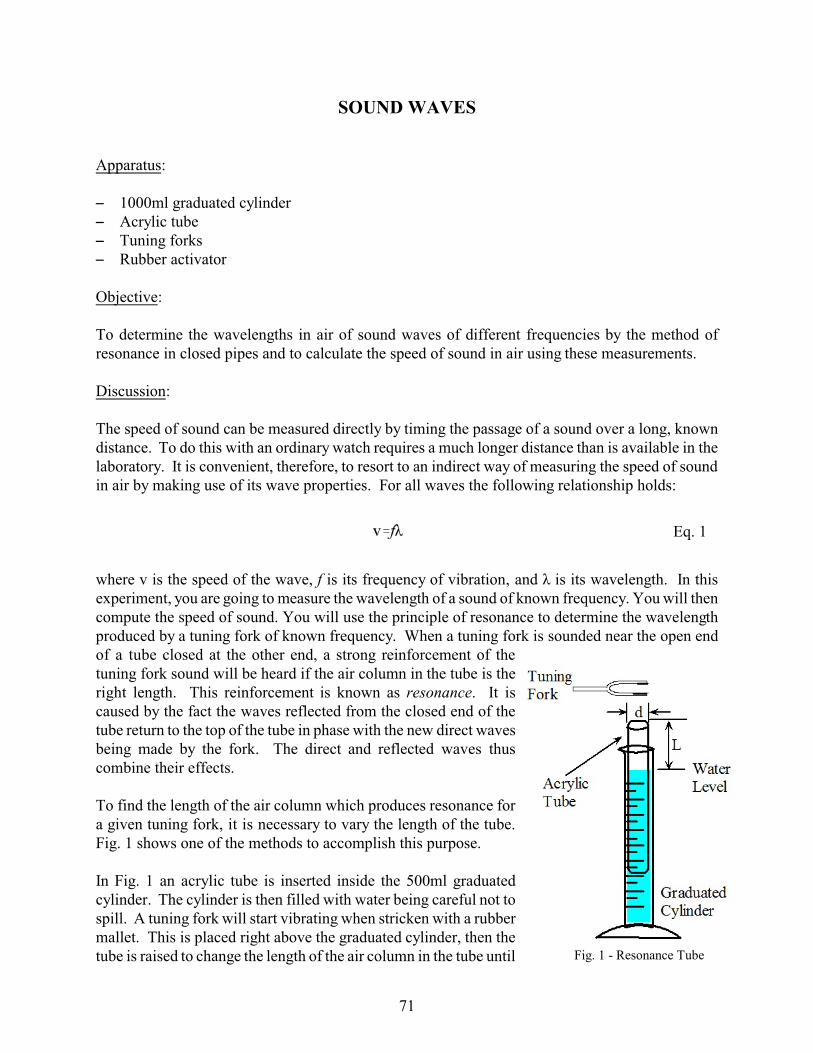
Eq. 1

SOUND WAVES

Apparatus:

S 1000ml graduated cylinderS Acrylic tubeS Tuning forksS Rubber activator

Objective:

To determine the wavelengths in air of sound waves of different frequencies by the method ofresonance in closed pipes and to calculate the speed of sound in air using these measurements.

Discussion:

The speed of sound can be measured directly by timing the passage of a sound over a long, knowndistance. To do this with an ordinary watch requires a much longer distance than is available in thelaboratory. It is convenient, therefore, to resort to an indirect way of measuring the speed of soundin air by making use of its wave properties. For all waves the following relationship holds:

where v is the speed of the wave, f is its frequency of vibration, and ë is its wavelength. In thisexperiment, you are going to measure the wavelength of a sound of known frequency. You will thencompute the speed of sound. You will use the principle of resonance to determine the wavelengthproduced by a tuning fork of known frequency. When a tuning fork is sounded near the open end of a tube closed at the other end, a strong reinforcement of thetuning fork sound will be heard if the air column in the tube is theright length. This reinforcement is known as resonance. It iscaused by the fact the waves reflected from the closed end of thetube return to the top of the tube in phase with the new direct wavesbeing made by the fork. The direct and reflected waves thuscombine their effects.

To find the length of the air column which produces resonance fora given tuning fork, it is necessary to vary the length of the tube. Fig. 1 shows one of the methods to accomplish this purpose.

In Fig. 1 an acrylic tube is inserted inside the 500ml graduatedcylinder. The cylinder is then filled with water being careful not tospill. A tuning fork will start vibrating when stricken with a rubbermallet. This is placed right above the graduated cylinder, then thetube is raised to change the length of the air column in the tube until Fig. 1 - Resonance Tube

71

Eq. 2

the sound intensity is at a maximum. For a tube closed at one end, whose diameter is smallcompared to its length, strong resonance will occur when the length of the air column is one-quarterof a wavelength, ë/4, of the sound waves made by the tuning fork. A less intense resonance will alsobe heard when the tube length is 3/4ë, 5/4ë, and so on.Since the shortest tube length for which resonance occurs is L=ë/4, it follows that ë. Practically, thisrelationship must be corrected for the diameter d of the tube. This gives:

In this experiment ë, L, and d will be measured in meters.

Procedure:

1. Measure the inner diameter of the hollow tube and record it.

2. Note the room temperature and record it as well.

3. Place the acrylic tube inside the graduated cylinder. Carefully, fill the graduated cylinder withwater . The water level should be as high as possible, making the air column as short as possible. Be careful not to spill water on the floor.

4. Choose a tuning fork of known frequency. Record the frequency.

5. Strike the tuning fork on the rubber activator and hold it over the open end of the tube. Hold thetuning fork so that the tines vibrate toward and away from the surface of the water in the cylinder(see Fig. 1). Slowly raise the tube until you hear strong resonance. At this point measure thelength of the air column in the tube L in meters and record it in your date table.

6. Repeat for other forks. If you are using tubes of different diameter make sure the new diameteris recorded too.

Table 1

Frequencyf

[Hz]

Length of AirColumn

L[m]

Diameter ofTube

d[m]

Wavelengthë

[m]

RoomTemperature

T[EC]

Speedv

[m/s]

72

Eq. 3

Calculations:

Using the values of L and d in Table 1, calculate the value of the wavelength ë from Eq. 2. Enterthis value of wavelength in the table.

1. Using Eq. 1 calculate the value of the speed of sound in air and record this value in the table foreach of the tuning forks used.

2. Calculate the value of the speed of sound in air from the following relation:

where T is the temperature in degrees centigrade and 331m/s is the speed of sound in air at 0EC.

3. Compare the result obtained by resonance measurement with the calculated value obtained byusing Eq. 3.

Questions:

1. How could you use the method and the results of this experiment to determine whether the speedof sound in air depends upon its frequency? What do your results indicate about such arelationship?

2. If we assume that the speed of sound at any temperature is known from Eq. 3, how can thisexperiment be used to measure the frequency of an unmarked tuning fork?

73

74

75

DETERMINING g ON AN INCLINE1

You have probably used the Behr Free Fall machine to determine the acceleration undergone by an object in free fall. Let us now use a different method to determine g. During the early part of the seventeenth century, Galileo experimentally examined the concept of acceleration. One of his goals was to learn more about freely falling objects. Unfortunately, his timing devices were not precise enough to allow him to study free fall directly. Therefore, he decided to limit the acceleration by using fluids, inclined planes, and pendulums. In this lab exercise, you will see how the acceleration of a rolling ball or cart depends on the ramp angle. Then, you will use your data to extrapolate to the acceleration on a vertical “ramp;” that is, the acceleration of a ball in free fall.

If the angle of an incline with the horizontal is small, a cart rolling down the incline moves slowly and can be easily timed. Using time and position data, it is possible to calculate the acceleration of the cart. When the angle of the incline is increased, the acceleration also increases. The acceleration is directly proportional to the sine of the incline angle, (θ ). A graph of acceleration versus sin(θ ) can be extrapolated to a point where the value of sin(θ ) is 1. When sinθ is 1, the angle of the incline is 90°. This is equivalent to free fall. The acceleration during free fall can then be determined from the graph. Galileo was able to measure acceleration only for small angles. You will collect similar data. Can these data be used in extrapolation to determine a useful value of g, the acceleration of free fall? We will see how valid this extrapolation can be. Rather than measuring time, as Galileo did, you will use a Motion Detector to determine the acceleration. You will make quantitative measurements of the motion of a cart rolling down inclines of various small angles. From these measurements, you should be able to decide for yourself whether an extrapolation to large angles is valid.

Fig. 1 - Set-up

OBJECTIVES • Use a Motion Detector to measure the speed and acceleration of a cart rolling down an incline. • Determine the mathematical relationship between the angle of an incline and the acceleration

of a cart rolling down the ramp. • Determine the value of free fall acceleration, g, by extrapolating the acceleration vs. sine of

track angle graph. • Determine if an extrapolation of the acceleration vs. sine of track angle is valid.

1 Adapted from Physics Vernier Manual.

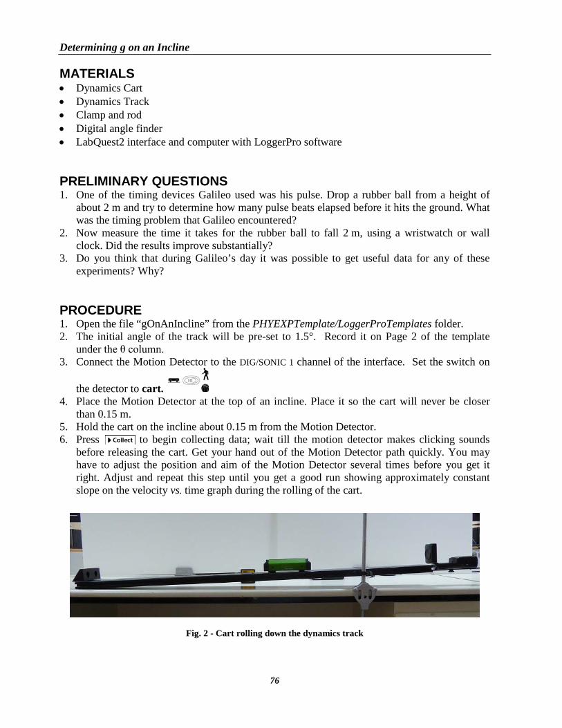
Determining g on an Incline

76

MATERIALS • Dynamics Cart • Dynamics Track • Clamp and rod • Digital angle finder • LabQuest2 interface and computer with LoggerPro software

PRELIMINARY QUESTIONS 1. One of the timing devices Galileo used was his pulse. Drop a rubber ball from a height of

about 2 m and try to determine how many pulse beats elapsed before it hits the ground. What was the timing problem that Galileo encountered?

2. Now measure the time it takes for the rubber ball to fall 2 m, using a wristwatch or wall clock. Did the results improve substantially?

3. Do you think that during Galileo’s day it was possible to get useful data for any of these experiments? Why?

PROCEDURE 1. Open the file “gOnAnIncline” from the PHYEXPTemplate/LoggerProTemplates folder. 2. The initial angle of the track will be pre-set to 1.5°. Record it on Page 2 of the template

under the θ column. 3. Connect the Motion Detector to the DIG/SONIC 1 channel of the interface. Set the switch on

the detector to cart. 4. Place the Motion Detector at the top of an incline. Place it so the cart will never be closer

than 0.15 m. 5. Hold the cart on the incline about 0.15 m from the Motion Detector. 6. Press to begin collecting data; wait till the motion detector makes clicking sounds

before releasing the cart. Get your hand out of the Motion Detector path quickly. You may have to adjust the position and aim of the Motion Detector several times before you get it right. Adjust and repeat this step until you get a good run showing approximately constant slope on the velocity vs. time graph during the rolling of the cart.

Fig. 2 - Cart rolling down the dynamics track

Determining g on an Incline

77

7. Logger Pro can fit a straight line to a portion of your data. First indicate which portion is to be used by dragging across the graph to indicate the starting and ending times. Then click on the Linear Fit button, , to perform a linear regression of the selected data. Use this tool to determine the slope of the Velocity vs. Time graph, using only the portion of the data for times when the cart was freely rolling. From the fitted line, find the acceleration of the cart. Record the value in your data table of Page 2 under the a column. Below is an example of data obtained with the motion detector and the fitted line to determine acceleration.

Fig. 3 – Sample Velocity graph and best-fit line representing acceleration.

8. Repeat Steps 6–7 two more times. 9. Raise the incline by adjusting the clamp and track till the digital angle finder reads

approximately 2.0°. Record the new angle in your data table. 10. Repeat Steps 6–8 for the new incline. 11. Repeat for 2.5°, 3.0°, 3.5° and 4.0°. ANALYSIS 1. Calculate the average acceleration for each angle. Plot a graph of the average acceleration vs.

sin(θ ). 2. Obtain a best-fit line using the linear fit feature of Logger Pro, and determine the slope. 3. How does the slope compare to the known value of g = 9.8 m/s2 ? 4. Plot a second graph same as in step 1 but change the x-axis so that it extends to 1.2 and the y-

axis so that it reaches 11. Obtain the best-fit, carry the fitted line out to sin (90°) = 1 on the horizontal axis, and read the value of the acceleration.2

5. How well does the extrapolated value agree with the accepted value of free-fall acceleration g = 9.8 m/s2?

6. Discuss the validity of extrapolating the acceleration value to an angle of 90°.

2 Notice that extrapolating to the y value at the x = 1 point is equivalent to using the slope of the fitted line.

Determining g on an Incline

78

79

PENDULUM STUDIES

1. DETERMINING PERIOD OF A PENDULUM BY MEANS OF A MOTION DETECTOR

OBJECTIVES • Use a motion detector to record the horizontal position vs time of a swinging pendulum. • Determine period of the pendulum motion. • Model the position data with a mathematical function and determine the period.

MATERIALS • Motion detector • Pendulum clamp and rod • Brass 2.5cm diameter pendulum bob with light string • Protractor, meter stick • Friction block • LabQuest2 interface and computer with LoggerPro software

PRELIMINARY SET-UP 1. Connect a motion detector to DIG1port of the labquest. Turn on the LabQuest2 interface

and connect it a computer via a USB cable. 2. Open the file “PendulumExtra” from the PHYEXPTemplate/LoggerProTemplates folder.

PROCEDURE 1. Clamp the 2.5cm diameter brass ball with length equal 0.50m. To ensure that the motion

detector captures the full swinging motion, the pendulum clamp should be positioned at a height of 0.55m from the table.

2. Slide the switch on the motion detector to the right to set the swith to the ball/walk setting. Place the detector atop a friction block and position them at a distance 0.40m away from the pendulum while it is at rest. Zero the sensor.

Fig.1 – Pendulum and Motion Detector Set-up

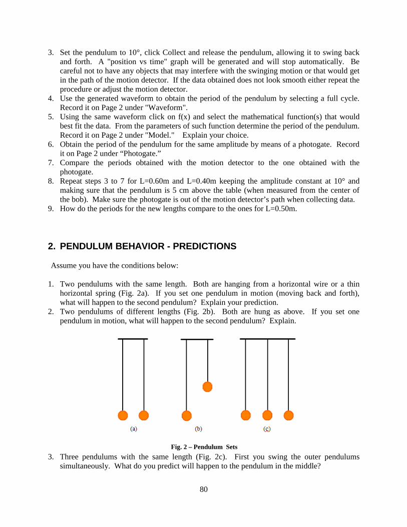
80

3. Set the pendulum to 10°, click Collect and release the pendulum, allowing it to swing back and forth. A "position vs time" graph will be generated and will stop automatically. Be careful not to have any objects that may interfere with the swinging motion or that would get in the path of the motion detector. If the data obtained does not look smooth either repeat the procedure or adjust the motion detector.

4. Use the generated waveform to obtain the period of the pendulum by selecting a full cycle. Record it on Page 2 under "Waveform".

5. Using the same waveform click on f(x) and select the mathematical function(s) that would best fit the data. From the parameters of such function determine the period of the pendulum. Record it on Page 2 under "Model." Explain your choice.

6. Obtain the period of the pendulum for the same amplitude by means of a photogate. Record it on Page 2 under “Photogate.”

7. Compare the periods obtained with the motion detector to the one obtained with the photogate.

8. Repeat steps 3 to 7 for L=0.60m and L=0.40m keeping the amplitude constant at 10° and making sure that the pendulum is 5 cm above the table (when measured from the center of the bob). Make sure the photogate is out of the motion detector’s path when collecting data.

9. How do the periods for the new lengths compare to the ones for L=0.50m.

2. PENDULUM BEHAVIOR - PREDICTIONS

Assume you have the conditions below:

1. Two pendulums with the same length. Both are hanging from a horizontal wire or a thin horizontal spring (Fig. 2a). If you set one pendulum in motion (moving back and forth), what will happen to the second pendulum? Explain your prediction.

2. Two pendulums of different lengths (Fig. 2b). Both are hung as above. If you set one pendulum in motion, what will happen to the second pendulum? Explain.

3. Three pendulums with the same length (Fig. 2c). First you swing the outer pendulums simultaneously. What do you predict will happen to the pendulum in the middle?

Fig. 2 – Pendulum Sets

81

4. If instead you swing the pendulum in the center while the other two remain at rest, what do you predict will happen after the pendulum is set in motion? Explain

5. You have a rectangular plate being held up from each corner (Fig. 3d), with each string being perfectly parallel to each other. The flat plate is set into motion sideways and time is recorded for 20 oscillations.

6. What if you cut the front strings from the flat plate pendulum allowing it to hang forward (Fig. 3e) and set it to motion again for 20 oscillaitons, what do you predict the period will be? Will it be the same as above? Why or why not. Explain.

7. Be prepared to put your predictions to the test!

Fig. 3 – Pendulum Flat Plate and Pendulum Hanging Plate

82

APPENDIX

83

84

85

A1. GRAPHICAL ANALYSIS 3.41

PLOTTING YOUR DATA POINTS AND FINDING THE BEST FIT

1. Click on the GA 3.4 icon

2. The Graphical Analysis screen will be displayed:

3. On the Data Set Table with X and Y columns

click on either column to start entering your

data. Use either the arrow keys or the mouse to

move to the next cell.

4. As you enter data you will notice a graph will

develop as the data is plotted. Just continue

entering your data till you are finished.

5. To delete the line that is connecting the points

either double click on the graph window. Select

the Graph Options tab.

1 Adapted from Vernier Software & Technology – Graphical Analysis User’s Manual

86

Click on Connect Lines to delete

the original line on your graph.

To add a title, click on the Title

window.

This window also gives the

option to add a legend to your

graph or change the grid style.

6. Finding the Best Linear Fit for

your graph:

On the graph window click and

drag the mouse across the

segment of interest. The shaded

area marks the beginning and end

of the range. You may also

select the segment of interest on your data columns and then clicking on the graph

window to activate it.

7. With the graph window activated, select the Regression option either by clicking the

Linear Fit icon, on the toolbar or by selecting it from the Analyze Menu. To remove

the regression line click the box in the upper corner of the helper object.

The Linear Fit function fits the line y = m*x + b to the selected region of a graph and

reports the slope (m) and y-intercept (b) coefficients. If more than one column or data

set is plotted, a selection dialog will open for you to which set you want to fit. You may

select more than one column for regression; in this case, a separate fit line will be applied

to each graphed column.

As aforementioned, you can fit a line either to the whole graph or to a region of interest.

Drag the mouse across the desired part of the graph to select it. Black brackets mark the

beginning and end of the range.

8. If you wish to graph a fit other than y=mx+b, such as proportional, quadratic, cubic,

exponential, etc, click on the Curve Fit icon from the toolbar. A Curve Fit

dialog window will pop-up:

87

Select the function you wish to use. Click Try Fit. Then click OK.

9. To change the labels of your X and Y axes and include their respective units click on the

column you wish to change and the dialog window below will pop-up:

On this dialog window, you will be allowed to give your column a name other than the

default name. You may also include units such as m/s, cm/s2, etc. The drop down arrows

allows you to enter a symbol, subscript or superscript.

10. To change the scaling of your graph, right click on the desired graph and select autoscale

or autoscale from zero. To modify manually, click on the highest or lowest number of

the axis you wish to change and enter the new number, press Enter.

88

11. Select the orientation of your page. This is done by using Page Setup under the File

menu.

12. To print the entire screen select Print from the File menu or click the icon on

the toolbar. A dialog window will pop-up allowing you to enter your name or

any comments you wish to add.

13. If you wish to print just the graph select it first and then go to the File menu and select

Print Graph… You may also print data table alone by selecting Print Data Table.

For more information go to: http://www2.vernier.com/manuals/ga3manual.pdf

Note: These basic graphing instructions can also be applied to LoggerPro.

89

A2. TECHNICAL NOTES ON VERNIER LABQUEST2 INTERFACE1

Once the LabQuest interface is connected to AC power or the battery has been charged, press the

power button located on the top of the unit, near the left edge. LabQuest will complete its

booting procedure and automatically launch the LabQuest App by default, as shown above. If the

screen momentarily shows a charge battery icon or does not light after a moment when used on

battery power, connect the power adapter to LabQuest and to an AC power source, then try the

power button again.

Power Button

Power on – If the screen is off for any reason (LabQuest is off, asleep, or the screen has

turned off to conserve battery power), press and release the power button to turn LabQuest

back on. If LabQuest was off, LabQuest will also complete its booting procedure that takes

about a minute and then display LabQuest App.

Sleep/wake – When LabQuest is on, press and release the power button once to put

LabQuest into a sleep mode. Note that the sleep mode does not start until you release the

power button. In this mode, LabQuest uses less power but the battery can still drain. This

mode is useful if you are going to return to data collection again soon, in which case waking

LabQuest from sleep is quicker than restarting after shutdown. To wake LabQuest from

sleep, press and release the power button. A LabQuest that is left asleep for one week will

automatically shutdown.

Shut down – To shut down LabQuest, hold the power button down for about five seconds.

LabQuest displays a message indicating it is shutting down. Release the power button, and

allow LabQuest to shut down. To cancel the shutdown procedure at this point, tap Cancel.

You can also shut down LabQuest from the Home screen. To do this, tap System and then

tap Shut Down.

Emergency shutdown – If you hold the power button down for about eight seconds, while it

is running. This is not recommended unless LabQuest is frozen, as you may lose your data

and potentially cause file system corruption.

1 Adapted from Vernier Software & Technology LabQuest2 User’s Manual.

Fig. 1 - LabQuest2 Interface

90

Touch Screen

LabQuest has an LED backlit resistive touch screen that quickly responds to pressure exerted on

the screen. LabQuest is controlled primarily by touching the screen. The software is designed to

be finger-friendly. In some situations, you may desire more control for precise navigation. In

such cases, we recommend using the included stylus.

If you are having trouble viewing the color screen or are using LabQuest outside in bright

sunlight, we recommend changing to the High Contrast mode. Tap Preferences on the Home

screen, then tap Light & Power. Select the check box for High Contrast to enable this mode.

Hardware Keys

In addition to using the touch screen, the three hardware keys can also be used to control your

LabQuest.

Collect – Start and stop data collection within LabQuest App

Home – Launch the Home screen to access other applications

Escape – Close most applications, menus, and exit dialog boxes without taking action (i.e.,

cancel dialog boxes)

Sensor Ports

LabQuest has three analog sensor ports (CH 1, CH 2, and CH 3) for analog sensors such as our

pH Sensor, Temperature Probe, and Force Sensor. Also included is a full-size USB port for USB

sensors, USB flash drives, and USB printers. In addition to the power button, the top edge of

LabQuest has two digital sensor ports (DIG 1 and DIG 2) for Motion Detectors, Drop Counters,

and other digital sensors.

Fig. 2 - LabQuest2 Control Buttons

Fig. 3- LabQuest2 Sensor Ports

91

Audio ports are also located adjacent to the digital ports, as well as a microSD card slot for

expanding disk storage. On the side opposite of the analog ports, there is a stylus storage slot, an

AC power port for recharging the battery, and a mini USB port for connecting LabQuest to a

computer. In between these ports, there is a serial connection for charging the unit in a LabQuest

Charging Station.

For more information on the LabQuest2 interface please go to:

http://www2.vernier.com/manuals/labquest2_user_manual.pdf

Fig. 4 - LabQuest2 Additional Ports

92

93

A3. TECHNICAL NOTES ON SENSORS AND PROBES UTILIZED IN SELECTED EXPERIMENTS FROM THIS MANUAL1

1. PHOTOGATES Photogates allow for extremely accurate timing of events within physics experiments, for studying air track collisions, pendulum periods, among other things. The PASCO ME-9215B Photogate Timer (Fig. 1) is an accurate and versatile digital timer for the student laboratory. The ME-9215B memory function makes it easy to time events that happen in rapid succession, such as an air track glider passing twice through the photogate, once before and then again after a collision.

The Photogate Timer uses PASCO’s narrow-beam infrared photogate (Fig. 2) to provide the timing signals. An LED in one arm of the photogate emits a narrow infrared beam. As long as the beam strikes the detector in the opposite arm of the photogate, the signal to the timer indicates that the beam is unblocked. When an object blocks the beam so it doesn’t strike the detector, the signal to the timer changes.

Timing Modes: • Gate Mode: In Gate mode, timing begins when the

beam is first blocked and continues until the beam is unblocked. Use this mode to measure the velocity of an object as it passes through the photogate. If an object of length L blocks the photogate for a time t, the average velocity of the object as it passed through the photogate was L/t.

• Pulse Mode: In Pulse mode, the timer measures the

time between successive interruptions of the photogate.

Timing begins when the beam is first blocked and continues until the beam is unblocked and then blocked

1 Technical notes adapted from Vernier Software & Technology User’s Manual and Pasco Scientific User’s Manual

Fig. 3 - Photogate timer with memory

Fig. 1 - Photogate timer with memory

Fig. 2 - Photogate head

94

again. With an Accessory Photogate plugged into the Photogate Timer, the timer will measure the time it takes for an object to move between the two photogates.

• Pendulum Mode: In Pendulum mode, the timer measures the period of one complete

oscillation. Timing begins as the pendulum first cuts through the beam. The timer ignores the next interruption, which corresponds to the pendulum swinging back in the opposite direction. Timing stops at the beginning of the third interruption, as the pendulum completes one full oscillation.

• Manual Stopwatch: Use the START/STOP button in either Gate or Pulse mode. In Gate

mode the timer starts when the START/STOP button is pressed and it stops when the button is released. In Pulse mode, the timer acts as a normal stopwatch. It starts timing when the START/STOP button is first pressed and continues until the button is pressed a second time.

• Memory Feature: When two measurements must be made in rapid succession, such as

measuring the pre- and post-collision velocities of an airtrack glider, use the memory function. It can be used in either the Gate or the Pulse mode. To use the memory: 1. Turn the MEMORY switch to ON. 2. Press RESET. 3. Run the experiment.

When the first time (t1 ) is measured, it will be immediately displayed. The second time (t2 ) will be automatically measured by the timer, but it will not be shown on the display.

4. Record t1 , then push the MEMORY switch to READ. The display will now show the TOTAL time, t1 + t2 . Subtract t1 from the displayed time to determine t2

2. SMART-PULLEY SYSTEM: A Smart-Pulley system is made up of a Vernier Ultra Pulley and a photogate to monitor motion as a string passes over a pulley. Note that the pulley has low friction and low inertia. When properly positioned, the spokes of the pulley will block the photogate’s infrared beam each time they pass by. In the Smart-Pulley systems one arm of the photogate emits a thin beam of infrared light which is detected by the other arm. The LabQuest2 interface discerns whether the beam strikes the detector (Fig. 4a) or is blocked by a spoke (Fig. 4b) in the pulley sheaf. The small LED light illuminates when the beam is blocked. By accurately timing the signals that arrive from the photogate, the computer is able to track the motion of any object linked to the pulley.

As the Smart-Pulley system performs motion timing it provides a Position vs Time graph; based on the data a Velocity vs Time graph can be developed as well as an Acceleration vs Time graph. For our experiment we will only be using the Velocity vs Time graph to obtain the required accelerations.

Fig. 4 – Smart-Pulley System

(a) (b)

95

3. MOTION DETECTOR The Motion Detector is used to collect position, velocity and acceleration data of moving objects. Students can study a variety of motions with the Motion Detector, including: • Walking toward and away from the Motion Detector. • Dynamics carts moving on track. • Objects in simple harmonic motion, such as a mass hanging on a

spring. • Pendulum motions. • Objects dropped or tossed upward. • A bouncing object.

How the Motion Detector Works This Motion Detector emits short bursts of ultrasonic sound waves from the gold foil of the transducer. These waves fill a cone-shaped area about 15 to 20° off the axis of the centerline of the beam. The Motion Detector then “listens” for the echo of these ultrasonic waves returning to it. The equipment measures how long it takes for the ultrasonic waves to make the trip from the Motion Detector to an object and back. Using this time and the speed of sound in air, the distance to the nearest object is determined.

Fig. 5 - Vernier Motion Detector

Fig. 6 - Sample motion data of a bouncing ball

Fig. 7 - Cone of action

96

Note that the Motion Detector will report the distance to the closest object that produces a sufficiently strong echo. The Motion Detector can pick up objects such as chairs and tables in the cone of ultrasound. The sensitivity of the echo detection circuitry automatically increases, in steps, every few milliseconds as the ultrasound travels out and back. This is to allow for echoes being weaker from distant objects. Features of the Motion Detector • The Motion Detector is capable of measuring objects as close as 0.15 m and as far away as 6

m. The short minimum target distance (new to this version of the Motion Detector) allows objects to get close to the detector, which reduces stray reflections.

• The Motion Detector has a pivoting head, which helps you aim the sensor accurately. For example, if you wanted to measure the motion of a small toy car on an inclined plane, you can lay the Motion Detector on its back and pivot the Motion Detector head so that it is perpendicular to the plane.

• The Motion Detector has a Sensitivity Switch (Fig. 8), which is

located under the pivoting Motion Detector head. To access it, simply rotate the detector head away from the detector body. Slide the Sensitivity Switch to the right to set the switch to the Ball/Walk setting. This setting is best used for experiments such as studying the motion of a person walking back and forth in front of the Motion Detector, a ball being tossed in the air, pendulum motion, and any other motion involving relatively large distances or with objects that are poor reflectors (e.g., coffee filters). The Track sensitivity setting works well when studying motion of carts on tracks like the Dynamics Cart and Track System, or motions in which you want to eliminate stray reflections from objects near to the sensor beam.

4. TEMPERATURE PROBE

The Stainless Steel Temperature Probe can be used as a thermometer for experiments in chemistry, physics, biology, Earth science, environmental science, and more. Note: Vernier products are designed for educational use. Our products are not designed nor recommended for any industrial, medical, or commercial process such as life support, patient diagnosis, control of a manufacturing process, or industrial testing of any kind.

Specifications: • Temperature range: –40 to 135°C (–40 to 275°F) • Maximum temperature that the sensor can tolerate without damage: 150°C

Fig. 8 - Sensitivity Switch

Fig. 9- Vernier Temperature Probe

97

• Typical Resolution: o .17°C (–40 to 0°C) o .03°C (0 to 40°C) o .1°C (40 to 100°C) o .25°C (100 to 135°C)

• Temperature sensor: 20 kΩ NTC Thermistor • Accuracy: ±0.2°C at 0°C, ±0.5°C at 100°C • Response time (time for 90% change in reading):

o 10 seconds (in water, with stirring) o 400 seconds (in still air) o seconds (in moving air)

• Probe dimensions: o Probe length (handle plus body): 15.5 cm o Stainless steel body: length 10.5 cm, diameter 4.0 mm o Probe handle: length 5.0 cm, diameter 1.25 cm

98