photovoltaic capacity valuation methods peak... · of photovoltaic capacity valuation methods and...
TRANSCRIPT

Tom Hoff, Clean Power Research
Richard Perez, State University of New York at Albany
JP Ross, Sungevity
Mike Taylor, Solar Electric Power Association
May 2008
PHOTOVOLTAIC CAPACITY VALUATION METHODS
SEPA REPORT # 02-08

May 2008
1
ACKNOWLEDGEMENTS This study was funded by the US Department of Energy as part of the Solar America Initiative under contract # DE-FC36-07GO17036 with the State University of New York – Albany and by the Solar Electric Power Association.
We wish to thank Tom Hansen at Tucson Electric Power for participating in discussions and letting us use excerpts of his study, as well as Kathleen Rutherford for leading the discussions and consensus building process at the workshop.
DISCLAIMER This report was prepared as an account of work sponsored by an agency of the United States Government. Neither the United States Government nor any agency thereof, nor any of their employees, makes any warranty, express or implied, or assumes any legal liability or responsibility for the accuracy, completeness, or usefulness of any information, apparatus, product or process disclosed, or represents that its use would not infringe privately owned rights. Reference herein to any specific commercial product, process, or service by trade name, trademark, manufacturer, or otherwise does not necessarily constitute or imply its endorsement, recommendation, or favoring by the United States Government or any agency thereof. The views and opinions of authors expressed herein do not necessarily state or reflect those of the United States Government or any agency thereof.

May 2008
2
TABLE OF CONTENTS Acknowledgements ......................................................................................................................... 1
Disclaimer ........................................................................................................................................ 1
Figures ............................................................................................................................................. 3
Tables .............................................................................................................................................. 3
Executive Summary ......................................................................................................................... 4
Introduction ...................................................................................................................................... 5
PV Capacity Valuation Methods ....................................................................................................... 6
Effective Load Carrying Capability (ELCC) .................................................................................. 6
Load Duration Magnitude Capacity (LDMC) ................................................................................ 8
Load Duration Time-based Capacity (LDTC) .............................................................................. 9
Solar-Load-Control-Based Capacity (SLC) ................................................................................ 10
Minimum-Buffer-Energy-Storage-based Capacity (MBESC) ..................................................... 11
Demand-Time Interval Matching (DTIM) ................................................................................... 12
Time/Season Windows (TSW) ................................................................................................... 13
Capacity Factor (CF) .................................................................................................................. 13
Comparison of Methods ................................................................................................................ 14
Geographical Dispersion and Time Sampling Intervals ................................................................ 15
A. Time Intervals ..................................................................................................................... 15
B. Installation(s); and C. Geography ...................................................................................... 16
D. Back-up/Storage .................................................................................................................... 17
Case Studies: Quantitative Examples ........................................................................................... 18
Discussion .................................................................................................................................. 20
Case Study Addendum: Demand-Time Interval Matching (DTIM) ............................................ 23
Logistical Issues ......................................................................................................................... 24
Variable Generating Capacity in Practice ...................................................................................... 25
Building Consensus ....................................................................................................................... 26
References .................................................................................................................................... 29
Appendix A: Technical Details ....................................................................................................... 30
Appendix B: Time Sampling .......................................................................................................... 34

May 2008
3
FIGURES Figure 1: Illustration of the ELCC method. ...................................................................................... 6 Figure 2: Relationship between ELCC and a utility’s summer-to-winter peak load ratio. ............... 7 Figure 3: Illustration of the LDMC method. ...................................................................................... 8 Figure 4: Illustration of the LDTC method.. ..................................................................................... 9 Figure 5: Illustration of Solar-Load-Control-based Capacity method. . ......................................... 10 Figure 6: Illustration of Minimum-Buffer-Energy-Storage-based Capacity method. .................... 11 Figure 7: Illustration of the Demand-Time Interval Matching method. .......................................... 12 Figure 8: Comparison of the normalized PV output of two nearby PV plants around Austin. ....... 16 Figure 9: Comparing all capacity credit metrics for Nevada Power.. ............................................ 19 Figure 10: Comparing all capacity credit metrics for Rochester Gas and Electric.. ...................... 19 Figure 11: Comparing all capacity credit metrics for Portland General. ........................................ 20 Figure 12: Comparing ELCC and LDTC metrics for 50 utilities. .................................................... 20 Figure 13: Illustrating the impact of the Garver Capacity Factor selection upon calculated ELCC
for Nevada Power at 10% PV grid penetration. ................................................................. 22 Figure 14: Illustrating the impact of the Garver Capacity Factor selection upon calculated ELCC
for Rochester Gas & Electric at 10% PV grid penetration. ................................................ 22 Figure 15: Illustrating the impact of the Garver Capacity Factor selection upon calculated ELCC
for Portland General at 10% PV grid penetration............................................................... 22 Figure 16: Springerville PV Plant DTIM Hourly Capacity Values for December 3, 2005. ............. 23 Figure 17: Comparison of satellite-derived to ground measured global irradiance in the vicinity of
Austin, TX. ........................................................................................................................ 24 Figure 18: Results of the straw poll on methodology preference. ................................................. 28 Figure 19: Power changes for PV plant in winter using 60 minute time intervals. ........................ 34 Figure 20: Power changes for PV plant in winter using 15 minute time intervals. ........................ 35 Figure 21: Power changes for PV plant in winter using 1 minute time intervals. .......................... 35 Figure 22: Power changes for PV plant in winter using 10 second time intervals. ....................... 36 Figure 23: One-minute irradiance and variability at one single location in the network ................ 37 Figure 24: One-minute irradiance and variability from 20 bundled network stations. ................... 38
TABLES Table 1: PV Capacity Methods Comparison Table ....................................................................... 14 Table 2: Wind Capacity Methods Comparison .............................................................................. 25 Table 3: Springerville PV Plant Output from 10:00am - 3:00pm on December 3, 2005. .............. 36

May 2008
4
EXECUTIVE SUMMARY
The U.S. Department of Energy’s Solar America Initiative provided funding to evaluate the variety of photovoltaic capacity valuation methods and to bring the solar industry, electric utility, and research communities together with the goal of building a consensus of the most appropriate PV generation capacity valuation method(s).1 Developing a framework for accurately and appropriately calculating photovoltaic capacity, and determining the risk of variation, will provide a means for utilities and generators to calculate and innovate around the new economic propositions that an industry recognized PV capacity value calculation method would present.
As part of the project, a draft of this paper was developed and distributed prior to a workshop held at the Solar Power 2007 conference, the discussion from which has been incorporated into this final document. The primary objective of the workshop was to introduce the PV capacity methods catalogued in the draft paper and create initial dialogue around them.
This final report is designed to give participants a background on the PV capacity methods and issues related to them, as well as a summary of the workshop. From the workshop, three methods were identified as more preferable – Effective Load Carrying Capacity, Solar Load Control / Minimum Buffer Energy Storage (combined as one due to similarities), and Demand Time Interval Matching. Subsequent work should likely focus on these three methods, along with further exploration of the effect of differing input variables. The work identified geography and time sampling, and their effects on the methods’ results, as two key input variables that must be more thoroughly investigated in a follow on phase of work.
1 Some of the proposed methods may be appropriate for capacity valuation at a building, distribution, or transmission level as well, but the scope here is limited to system-level capacity.

May 2008
5
INTRODUCTION
Maintaining adequate generating capacity to meet electricity demand at all times is a fundamental principle for the electric utility industry. This is accomplished through a variety of means including providing/purchasing sufficient generation capacity as well as acquiring the associated ancillary services for the electricity grid.
The generation capacity of dispatchable resources is assessed based on technology design parameters. While dispatchable resources have some uncertainty in their output due to unforeseen equipment failures, their dispatch is managed around the demand for electricity and their marginal operating costs.
Photovoltaic resources are non-dispatchable because their electrical output is based on both technology design parameters (technology selection, installation characteristics, and site conditions) and a solar resource that varies over a range of time periods (seasonal, daily, hourly, second to second). These solar resource variations, however, are not random and there is an intuitively positive relationship between PV system output and summer peak electricity demand for many locations throughout the U.S. This is because system demand peaks for most utilities are driven by heat-wave cooling demand, and because heat waves are indirectly fed by solar gain, i.e., by the fuel for PV generation.
Despite this relationship, there is no consensus across the utility or solar industries on a method for calculating PV capacity or its practical use in electricity markets and utility planning.
There are two operational definitions that need to be distinguished as part of identifying various capacity valuation methods.
1. A capacity method is a specific mathematical model (formula) for calculating a PV capacity value.
2. Each method may have different input variables, such as electric system demand, PV capacity and performance, time parameters, number of installations, geography, and/or back-up/storage.2
Different input variables, such as minute or hourly time intervals, will significantly affect the results of even the same method. The project’s scope is to focus on methods, which each may include different input variables, but was not designed to focus on what parameter level to set these input variables.
2 While the sampling interval of input variables is critical to a method’s results, they are not necessarily tied to any particular method. Regional, state, regulatory, or utility preferences is the most likely forum for adopting specific sampling intervals.

May 2008
6
PV CAPACITY VALUATION METHODS This section briefly discusses eight PV capacity methods that have been identified. Effective Load Carrying Capability (ELCC) The ELCC metric was introduced by Garver in 1966 [1] and has been used mainly by “island” utilities before the strengthening of continental/regional interconnectivity. The method was applied at Pacific Gas and Electric Company [7]. The ELCC of a power plant represents its ability to increase the total generation capacity of a local grid (e.g., a contiguous utility’s service territory) without increasing its loss of load probability. The ELCC is determined by calculating the loss of load probability (LOLP) for two resources. The first resource is the actual resource with its time-varying output. The second resource is an “equivalent” resource with a constant output. The details of how to calculate the ELCC are presented in the Appendix.
The ELCC may be graphically visualized on a load duration curve plot. The example presented in Figure 1 -- using load data from Rochester Gas and Electric and a PV penetration X/L = 20% (see case studies below) -- shows the utility load duration curve with and without PV, and also shows the load duration curve obtained with a constant output generator with an ELCC capacity calculated at 145 MW for this case study (see quantitative case studies below).
Figure 1: Illustration of the ELCC method. Comparing load duration curves with and without PV to an equivalent load duration curve assuming a constant
output generator with an ELCC capacity. The example below is given for Rochester Gas and Electric (peak load = 1561 MW) and a PV penetration of 20% (312 MW). The ELCC calculated for this case figure is 47% (146 MW).
1,000
1,100
1,200
1,300
1,400
1,500
1,600
Top of the load duration curve
load
(MW
)
load duration without PV
load duration with PV at 20% penetration
Load duration with ELCC capacity installed

May 2008
7
It has also been shown that ELCC could be estimated from simple proxy measurements of local characteristics, such as a utility’s summer-to-winter peak load ratio (see Fig. 2).
Figure 2: Relationship between ELCC and a utility’s summer-to-winter peak load ratio.
0%
20%
40%
60%
80%
100%
0.5 0.7 0.9 1.1 1.3 1.5 1.7 1.9
SWPR
ELCC
(2ax
is-2
%)
elcc-2002/2003 dataelcc 1987/91 data1987/91 best fit2002/2003 best fit

May 2008
8
Load Duration Magnitude Capacity (LDMC) For this metric, the load duration curve is analyzed directly.
The LDMC parameter is defined as the mean PV output for all loads greater than the LDMC threshold defined as the utility’s peak load L, minus the installed PV capacity X, per equation (2).
LDMC threshold = L (1-p) (2)
Where L is the considered grid’s peak load and p is the PV penetration fraction, defined here as X / L.
The LDMC parameter is illustrated in Fig. 3. It directly accounts for PV penetration.
Figure 3: Illustration of the LDMC method.
40%
50%
60%
70%
80%
90%
100%
p
8760 hours
LDMC = average relative PV output for these points
LDMC = average relative PV output for these pointsS
orte
d lo
ads
rela
tive
to p
eak
load

May 2008
9
Load Duration Time-based Capacity (LDTC) The LDTC is defined as the average PV output during the n highest loads.
This metric is similar to the LDMC except for the definition of penetration p’, which is defined here in terms of time rather than in terms of size per equation 3.
LDTC threshold = nth ranked load (3)
Where n is defined by the considered penetration
n = p’N (4)
Where N is the total number of load points in the load duration curve.
For instance considering a yearly set of hourly loads (N = 8760), a 10% penetration would set the threshold at the 876th highest hourly load.
This parameter is illustrated in Figure 4. It also accounts for grid penetration, but indirectly, as the time dimension is used as a proxy for capacity.
Figure 4: Illustration of the LDTC method.
40%
50%
60%
70%
80%
90%
100%
0% 20% 40% 60% 80%
p’
LDTC = average relative PV output for these points
LDTC = average relative PV output for these points
Sor
ted
load
s re
lativ
e to
pea
k lo
ad
May 2008
10
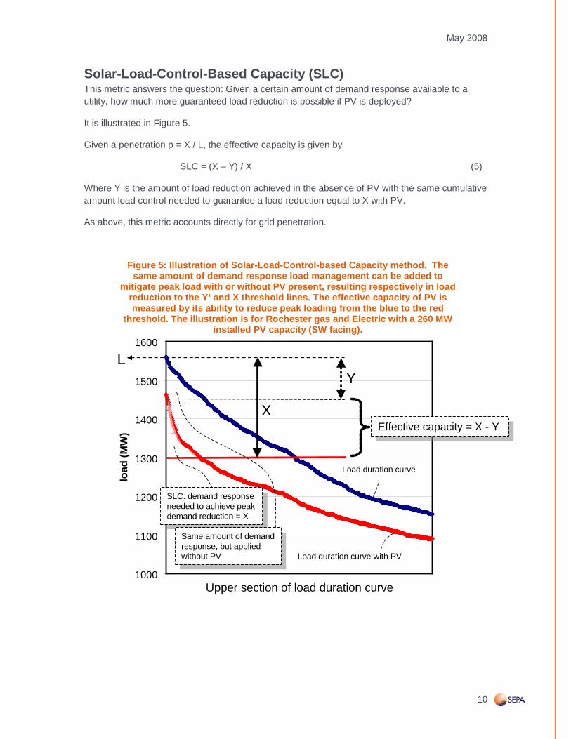
Solar-Load-Control-Based Capacity (SLC) This metric answers the question: Given a certain amount of demand response available to a utility, how much more guaranteed load reduction is possible if PV is deployed?
It is illustrated in Figure 5.
Given a penetration p = X / L, the effective capacity is given by
SLC = (X – Y) / X (5)
Where Y is the amount of load reduction achieved in the absence of PV with the same cumulative amount load control needed to guarantee a load reduction equal to X with PV.
As above, this metric accounts directly for grid penetration.
Figure 5: Illustration of Solar-Load-Control-based Capacity method. The same amount of demand response load management can be added to
mitigate peak load with or without PV present, resulting respectively in load reduction to the Y’ and X threshold lines. The effective capacity of PV is measured by its ability to reduce peak loading from the blue to the red
threshold. The illustration is for Rochester gas and Electric with a 260 MW installed PV capacity (SW facing).
1000
1100
1200
1300
1400
1500
1600
500 sorted highest loads
load
(MW
)
X
LY
Load duration curve
Load duration curve with PV
SLC: demand response needed to achieve peak demand reduction = X
SLC: demand response needed to achieve peak demand reduction = X
Same amount of demand response, but applied without PV
Same amount of demand response, but applied without PV
Upper section of load duration curve
Effective capacity = X - Y Effective capacity = X - Y
May 2008
11
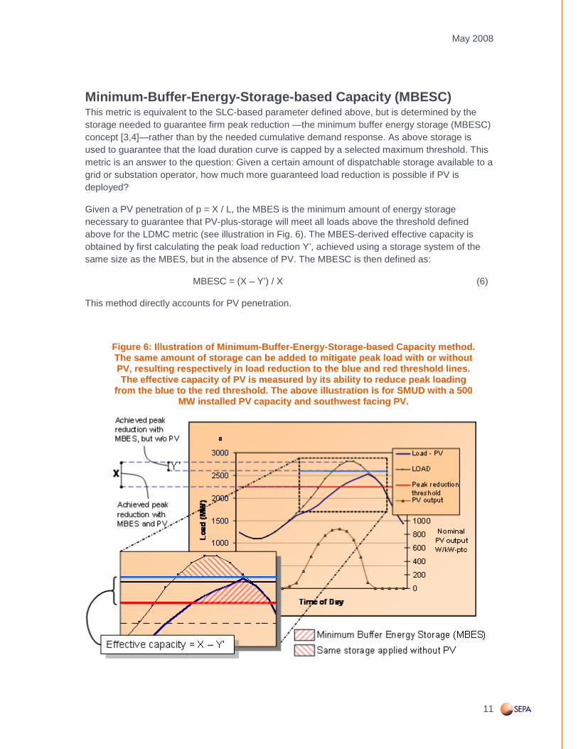
Minimum-Buffer-Energy-Storage-based Capacity (MBESC) This metric is equivalent to the SLC-based parameter defined above, but is determined by the storage needed to guarantee firm peak reduction —the minimum buffer energy storage (MBESC) concept [3,4]—rather than by the needed cumulative demand response. As above storage is used to guarantee that the load duration curve is capped by a selected maximum threshold. This metric is an answer to the question: Given a certain amount of dispatchable storage available to a grid or substation operator, how much more guaranteed load reduction is possible if PV is deployed?
Given a PV penetration of p = X / L, the MBES is the minimum amount of energy storage necessary to guarantee that PV-plus-storage will meet all loads above the threshold defined above for the LDMC metric (see illustration in Fig. 6). The MBES-derived effective capacity is obtained by first calculating the peak load reduction Y’, achieved using a storage system of the same size as the MBES, but in the absence of PV. The MBESC is then defined as:
MBESC = (X – Y’) / X (6)
This method directly accounts for PV penetration.
Figure 6: Illustration of Minimum-Buffer-Energy-Storage-based Capacity method. The same amount of storage can be added to mitigate peak load with or without PV, resulting respectively in load reduction to the blue and red threshold lines. The effective capacity of PV is measured by its ability to reduce peak loading
from the blue to the red threshold. The above illustration is for SMUD with a 500 MW installed PV capacity and southwest facing PV.

May 2008
12
Demand-Time Interval Matching (DTIM) The Demand-Time Interval Matching method has been pioneered by Tom Hansen based on Tucson Electric Power’s (TEP) experience with a single central station PV plant located several hundred miles from TEPs load center. The details of this method are summarized in the Appendix and can be accessed in detail by a forthcoming report.
The essence of this method is illustrated in Figure 7. This method examines the worst-case output of the PV system by subtracting the PV system output from the load (in TEPs case this is done over 10 second time intervals) and the capacity value is based on the worst-case difference between the load duration curve over the dispatch sampling interval.
Figure 7: Illustration of the Demand-Time Interval Matching method.
Top of the load duration curve
LOA
D
load duration without PVload duration with PV
Top of LD curve w/o PV
Top of LD curve with PV
X = installed PV Capacity≈ MaxSolarPowerDC
Z = difference between tops of LD curves ≈ MinSolarPowerDC
Capacity Credit= Z / X
Capacity Credit= Z / X
Load Duration Curves with Time Resolution Equalto Dispatch Sampling Interval

May 2008
13
Time/Season Windows (TSW) The Time/Season Window (TSW) method calculates capacity credits across predefined hours, months, and/or seasons. It is often cited as the ERCOT method derived from the practice to assign capacity credit to wind generators operating in the ERCOT regional reliability council. This practice is also used by MAPP.
There are at least two variations on the calculation. The ERCOT method predefines a peak demand time frame—e.g., May-October 10am -6PM—and defines capacity as the minimum output likely to occur with a probability α (α = 8 in the case of ERCOT-wind). MAPP utilizes a median capacity value across a monthly four hour window.
We examine here two possible representations of this approach: in the first representation, the peak time frame is defined by a predefined number of ranked peak demand days (TSWpeak); in the second representation, the peak time window is defined by a preset time period (TSWtime).
The TSW method does not account for grid penetration.
Capacity Factor (CF) The capacity factor quantifies a power plant’s average output relative to its installed capacity. This factor does not bear any relation to the load served and, of course, cannot account for grid penetration. However, this common measure of PV output may conceivably be used to quantify PV capacity.

May 2008
14
COMPARISON OF METHODS
Table 1: PV Capacity Methods Comparison Table
Attributes Methods
Impo
rtanc
e
ELC
C
LDM
C
LDTC
MB
ES
C
SLC
TSW
(pea
k/tim
e)
CF
DTI
M
PROCESS
Simple to implement
Simple to describe
Based on concepts familiar to utilities
Produces results that are consistent with other metrics that account for PV penetration
Has been implemented by utilities
SUBSTANCE
Based on actual PV output/load correlation
Accounts for PV penetration
Accounts for effect over all hours
Based on load duration curve
Can be used to perform worst case analysis and addresses short term variability issues
Provides operational measure of firm capacity when back-up/storage is available
Is deterministic (rather than statistical)

May 2008
15
GEOGRAPHICAL DISPERSION AND TIME
SAMPLING INTERVALS
Sample intervals are critically important to a method’s results, and are about “how” the method is applied, not the method itself. Much of the debate about PV capacity methods is actually about sample intervals rather than methods, and utilizing the same sample intervals may yield similar results across methods. The four most important input variables affecting method results are:
A. Time Intervals – the length of the time intervals for capturing and analyzing the data, i.e. 10 seconds or 1 hour.
B. Installation(s) – whether and how to incorporate two or more distinct PV installations. C. Geography – the geographic area for analyzing two or more PV installations, i.e. 25
mile radius, utility service territory, etc. D. Back-up/Storage – whether and how to incorporate the synergy of on-site or
purchased back-up generation, storage, or demand-response services to firm up PV performance
A. Time Intervals Although not fully analyzed in the scope of this paper, there may be some combination of different sampling intervals across the first three input variables that result in the same capacity value. For example
Time(10 seconds) + Installations(5 installations) + Distance(25 miles) =
Time(15 minutes) + Installations(1 installation) + Distance(0 miles)
Future research should further investigate this question across different methods, input variables, and sampling intervals.
While the goal of this project is to focus on methods, the choice of how to apply sample intervals will most likely remain a matter of local jurisdiction, i.e. utility, ISO, regulatory, etc.
The utility industry generally breaks the generation capacity requirements into two components, system firm generating capacity over some measure of peak demand and ancillary services over all or high demand hours, each with separate wholesale markets in some ISO jurisdictions. The window through which PV capacity is calculated, and whether the method is calculating system planning capacity benefit or ancillary capacity cost depends on the time interval and geographic framework being analyzed, i.e. system, service territory, feeder, etc.

May 2008
16
The wind industry, having a much larger grid penetration level, has studied wind grid integration extensively3. Wind installations can at the same time have an ISO system planning capacity as a percentage of rated capacity, as well as an average annual or monthly cost in cents per kilowatt-hour for these ancillary services that are generally being passively absorbed by the utility4. The economic question is then twofold: what is the capacity benefit of a given or aggregation of solar generators and what is the ancillary services cost for reliable integration of that solar resource into a given generation portfolio? Other questions regarding how those costs should be allocated by stakeholder (utility, generator, ISO, etc) or installation type or size (commercial, residential, large, small, etc) are a policy decision.
B. Installation(s); and C. Geography The statistical calculation of photovoltaic capacity can be altered by the distributed nature of photovoltaics and the potential statistical risk mitigation benefits that geographic diversity and the aggregation of performance across geographies could provide. This issue is important for short-term output variability. Five PV plants across a 50 mile area may have a lower risk of minute-by-minute capacity variation than one single plant, and could be a reasonable assumption for determining a contribution to overall system capacity planning if load and weather patterns are not correlated.
Figure 8 compares two normalized PV systems operating five miles apart in Austin, Texas [6]. The degree of scatter indicates that the output of the two plants can be quite different during partly cloudy conditions, therefore dampening any short term variability at any one location.
Figure 8: Comparison of the normalized PV output of two nearby PV plants around Austin, TX [6].
3 It should be noted that wind and solar technologies have different short-interval generating characteristics and are not necessarily comparable, i.e. turbine blade inertia as wind speeds slow versus the photovoltaic effect as cloud events occur. 4 For more information on wind integration studies: http://www.uwig.org/opimpactsdocs.html

May 2008
17
D. Back-up/Storage Back-up, storage, or demand-response technologies (generally “storage” hereafter) can be utilized to improve the performance of a PV system on the generator or utility side of the meter and some PV capacity methods discussed here can more seamlessly integrate this feature as an option, utilizing it if available or estimated at the user’s discretion. Storage, with or without PV, could theoretically be used to provide either ancillary services on a constant basis to remove or minimize these short-term fluctuations, or provide additional generating capacity benefits over critical peak hours. The same amount of storage may be able to be used more efficiently in tandem with PV rather than without to displace peak loads.

May 2008
18
CASE STUDIES: QUANTITATIVE EXAMPLES These case studies are based on the analysis of experimental hourly system load demand and PV generation data. They are designed to provide quantitative support to compare the methods in the context of utility-wide multi-locational dispersed PV generation.
Three utilities were selected with distinct characteristics. We analyzed one year of load data (2002) for each using sampling rates of one hour. Utility-specific 2002 PV outputs were simulated from satellite data.
The selected utilities are:
Nevada Power (NP) Rochester Gas and Electric (RG&E) Portland General (PG)
Nevada Power (NP) is a metropolitan utility in an arid western state, with considerable solar resource and a large commercial air-conditioning demand. NP is a summer peaking utility by a wide margin – its summer-to-winter peak load ratio was 1.93 in 2002.
Rochester Gas and Electric (RG&E) serves a medium-sized industrial city in upstate New York, where cloudy conditions are not infrequent. The utility also peaks in summer, with peaks driven by daytime industrial and commercial air conditioning, but not to the same extent as NP. RG&E’s summer-to-winter ratio was 1.32 in 2002.
Portland General serves the city of Portland, Oregon and vicinity. It has been a winter peaking utility until recent years, but now experiences more frequent summer peaks due to increased air conditioning demand and a general climatic trend to warmer summers. PG’s summer-to-winter peak ratio was 1.01 in 2002. Note, however, that winter energy consumption is still higher.
PV output was simulated for fixed systems facing southwest at 30o tilt, with penetrations ranging from 1% to 20% for each utility. As mentioned above, installed PV capacity is quantified in terms of ac-ptc conditions.
Comparative results for all metrics are presented in Figures 15, 16 and 17 for NP, RG&E and PG, respectively.

May 2008
19
Figure 9: Comparing all capacity credit metrics for Nevada Power as a function of the amount of PV on the grid from 1% of peak (~55 MW) up to 20% of peak (~1,100 MW).
0%
20%
40%
60%
80%
100%
0% 5% 10% 15% 20%
Grid penetration
Effe
ctiv
e C
apac
ityELCC LDMCLDTC SLCMBESC TSWpeakTSWtime CFDTIM
Figure 10: Comparing all capacity credit metrics for Rochester Gas and Electric as a function of the amount of PV on the grid from 1% of peak (~16 MW) up to 20% of peak
(~320 MW).
0%
20%
40%
60%
80%
100%
0% 5% 10% 15% 20%
Grid penetration
Effe
ctiv
e C
apac
ity
ELCC LDMCLDTC SLCMBESC TSWpeakTSWtime CFDTIM

May 2008
20
Figure 11: Comparing all capacity credit metrics for Portland General as a function of the amount of PV on the grid from 1% of peak (~35 MW) up to 20% of peak (~700 MW).
0%
20%
40%
60%
80%
100%
0% 5% 10% 15% 20%
Grid penetration
Effe
ctiv
e C
apac
ityELCCLDMCLDTCSLCMBESCTSWpeakTSWtimeCFDTIM
Discussion The most striking observation is that all the metrics that are based on a physical measure of PV penetration—ELCC, LDMC, MBESC, SLC and DTIM—provide similar measures of capacity credit. The highest divergence is observed for low penetration in Portland, where capacity credit is, in any case, marginal. The metric defining penetration in terms of time (LDTC) is a little more conservative, reflecting the fact that load duration curves tend to have a marked high-end peak driven by a small number of high-stress occurrences. This observation is based on three case studies, but the data presented in Figure 12, extrapolated from the results of an earlier analysis of ~ 50 utilities [3] for two of the metrics analyzed here (ELCC and LDTC), do show a strong agreement between load duration based metrics and ELCC.
The TSW metrics provide a considerably different measure of capacity credit, showing no dependence on penetration and are unreflective of any load-PV relationship. This is understandable because within an arbitrarily predefined peak time window, there are many occurrences where the load is small and when reliance on PV output is not critical. Even though there is a significant probability (8% in case of the ERCOT metric) that PV output could be low during this predefined window, this occurs at a time when the load is far from its physical peak. It is thus arguable that the TSW metric is not an appropriate measure of PV capacity credit - no more than the capacity factor should me a measure of capacity credit.
Figure 12: Comparing ELCC and LDTC metrics for 50 utilities using data from [3]. Data points are for two axis-tracking PV at 2% grid penetration.

May 2008
21
0%
20%
40%
60%
80%
100%
0% 20% 40% 60% 80% 100%
ELCC
LDTC
Selecting between the four physical penetration-based metrics is not a critical choice, because they do provide comparable estimates of capacity credit. The authors have a preference for either SLC or MBESC, because these measures introduce the concept of firm (100%) reliability when PVs are operated in tandem with either short term storage (MBESC) or demand response programs (SLC) already (or independently) available to utilities. However, there is a positive benefit from, and additional cost for the storage or demand response. Evaluating capacity with and without storage will provide a clear understanding of the net capacity and economic costs and benefits.
The ELCC offers a slightly more conservative estimate of capacity. However, one of the factors defining this metric, the Garver capacity factor m, is an unknown that would have to be locally determined, or standardized across the board - a value of m = 3% of peak load was selected for these case studies. Figures 19, 20 and 21 show how ELCC may vary as a function of the choice of m. Recall that m represents the load increase that leads to an augmentation of the loss of load probability by a factor of “e” ~ 2.7. When m is very large, the utility can absorb sizeable load increases without much of a loss of load probability increase and therefore does not need to critically rely on the new power generation (PV). Hence, the ELCC tends towards the value of the capacity factor, which is a measure of the average resource availability. On the other hand, very low values of m indicate high risk increase per small load increase. The peak in the Rochester curve, and the absence of peak in the Las Vegas curve, are an indication of cloudiness prevalence - conditions are predominantly clear in Vegas and any small load increases are captured by PV. In Rochester, although load and PV are highly correlated, some small peaks may experience partial cloudiness.

May 2008
22
The DTIM metric shows more discontinuity than other metrics when plotted against penetration; this is likely because it is based on one single critical point at the top of the load duration curve.
Figure 13: Illustrating the impact of the Garver Capacity Factor selection upon calculated ELCC for Nevada Power at 10% PV grid penetration.
0%10%20%30%40%50%60%70%80%
0.0% 10.0% 20.0% 30.0% 40.0% 50.0% 60.0%
Garver Capacity m relative to peak load
ELCC at 10% grid penetration
Figure 14: Illustrating the impact of the Garver Capacity Factor selection upon calculated
ELCC for Rochester Gas & Electric at 10% PV grid penetration.
0%10%20%30%40%50%60%70%
0.0% 10.0% 20.0% 30.0% 40.0% 50.0% 60.0%
Garver Capacity m relative to peak load
ELCC at 10% grid penetration
Figure 15: Illustrating the impact of the Garver Capacity Factor selection upon calculated
ELCC for Portland General at 10% PV grid penetration.
0%
5%
10%
15%
20%
25%
0.0% 10.0% 20.0% 30.0% 40.0% 50.0% 60.0%
Garver Capacity m relative to peak load
ELCC at 10% grid penetration

May 2008
23
Case Study Addendum: Demand-Time Interval Matching (DTIM) Based on Very Short Term Sampling The case studies presented above are based on hourly data analysis and co-location of demand and generation. The use of hourly data is deemed appropriate for system-wide load and generation spanning a wide enough footprint washing out short term fluctuations.
As a contrast to these case studies, we present below an excerpt of Tom Hansen’s analysis quantifying capacity credit when PV generation occurs at single location (Springerville, AZ) located 260 km distance from its load center [10]. The centralized PV generation implies that short term fluctuations are important, while the distance negates the natural feedback existing between peak demand and solar resource.
Figure 22 is a graph of the 4.6 MWp DC capacity rated Springerville Generating Station Solar System (SGSSS) minimum solar generation with SI = 10 seconds, DC = 1 hour and EP = 1 day in the middle of the winter (December 3, 2005). These data points are then compared with hourly system load data for that date to perform a full capacity credit evaluation. While a daily Evaluation Period does not make much sense when compared to the general lifecycle of weather patterns, it is instructive to note that the maximum hourly load, MaxLoadEP, for December 3, 2005 was 1,123.1 MW and occurred at hour ending 18:00, a dispatch cycle for which the minimum solar generation output was zero. With MaxSolarPowerEP of 4.6 MW for the EP, BaseLoadEP = 1123.1 – 4.6 = 1118.5 MW. As the second highest hourly system load for December 3, 2005 was 1117.0 MW, the only Dispatch Cycle comparison that would be made for capacity credit evaluation was at the 18:00 hour ending. Using this minimum sample interval solar output method to evaluate the SGSSS capacity credit, the capacity credit was 0.0 MW.
Figure 16: Springerville PV Plant DTIM Hourly Capacity Values for December 3, 2005.
SGSSS One Day (12/3/2005) Evaluation Period of Hourly Capacity Value;10 Second Sample Intervals; Basis Criteria: Minimum Generation During One Hour Dispatch
Periods
0%5%
10%15%20%25%30%35%40%45%50%55%60%65%70%75%80%85%90%95%
100%
7:00 8:00 9:00 10:00 11:00 12:00 13:00 14:00 15:00 16:00 17:00 18:00 19:00
60 Minute Period Ending
Min
imum
Eva
luat
ion
Perio
d G
ener
atio
n in
% o
f N
amep
late
Rat
ing
Minimum Hourly Sample Interval Generation

May 2008
24
Logistical Issues Time series of both actual PV generation and load data are required. In the examples presented in this report, we have used one year of hourly load and PV output time series. Load data were actual measurements of system-wide loads, but PV data were simulated from time/site-specific satellite data. PV generation was inferred through two models: (1) a satellite-to-irradiance model and (2) an irradiance-to-PV output model. The DTIM was an exception as it used actual 10 second PV output data and one minute load data. Current practice in Europe [5] and research in the US shows that in some cases this approach is versatile and reliable. Short of having access to comprehensive system-wide PV output data and/or appropriate system-wide irradiance measurements, this estimation method has proven consistent with actual results in certain, but not all, locations.
Figure 17: Comparison of satellite-derived to ground measured global irradiance in the vicinity of Austin, TX over a 10x10 km square [6].
However, for shorter time sampling intervals, satellite data is not available for estimating PV output and either on-site or local reference systems would need to be utilized.
For new PV systems with no operating record, historical proxy data from other locations could be utilized in the interim, until an operating history has been established.
Small PV systems may find that highly detailed on-site data monitoring is economically impractical, but in the aggregate, the sum of many of these systems provides a measurable capacity for system planning.

May 2008
25
VARIABLE GENERATING CAPACITY IN
PRACTICE The wind industry, being at a much larger penetration scale within the electric grid, has more practical examples of variable generating capacity being utilized by utilities and system operators for generation resource planning. An article in the Electricity Journal in 2006 [8] provided a summary of the practical status of wind capacity credits, which may provide a framework for discussions in the solar industry.
Table 2: Wind Capacity Methods Comparison Region/Utility Method Note
CA/CEC ELCC Rank bid evaluations for RPS (low 20s)
PJM Peak period Jun-Aug HE 3 p.m.–7 p.m., capacity factor using 3-year rolling average (20%, fold in actual data when available)
ERCOT 10% May change to capacity factor, 4 p.m.–6 p.m., (2.8%)
MN/DOC/Xcel ELCC Sequential Monte Carlo (26–34%)
GE/NYSERDA ELCC Offshore/onshore (40%/10%)
CO PUC/Xcel ELCC PUC decision (30%) and Current Enernex study possible follow-on; Xcel using MAPP approach (10%) in internal work
RMATS Rule of thumb 20% all sites in RMATS
PacifiCorp ELCC Sequential Monte Carlo (20%)
MAPP Peak period Monthly 4-hour window, median
PGE 33% (method not stated)
Idaho Power Peak period 4 p.m.–8p.m. capacity factor during July (5%)
PSE & Avista Peak period PSE will revisit the issue (lesser of 20% or 2/3 Jan C.F.)
SPP Peak period Top 10% loads/month; 85th percentile
Source: Milligan, Michael and Kevin Porter. “The Capacity Value of Wind in the United States: Methods and Implementation.” The Electricity Journal. March 2006, Vol. 19, Issue 2

May 2008
26
BUILDING CONSENSUS The first step taken towards building consensus was the presentation and discussion of a draft of this report at the PV Capacity Workshop held during the SEPA/SEIA Solar Power 2007 conference. The workshop was followed by other online and live presentations that further refined the process and strengthened consensus.
Our primary objective at the workshop was to achieve introduce the PV capacity methods identified—focusing on the method rather than on the related input variables, such as time/geography and operational data issues, while recognizing their importance, their interdependence, and the need to subsequently address them.
The workshop was designed to help participants:
1. Review the PV capacity methods. 2. Qualitatively compare the merits of the various methods. 3. Discuss sampling intervals and the relationship with geographical dispersion. 4. Discuss the practical applications for the methods and sampling intervals.
Discuss follow-up activities from the workshop.Focusing on the methods alone was a challenge because the question of capacity itself brings related issues to the table. Although important, their relevance to the method selection may be secondary.
The issues discussed during the workshop included:
The monetary value of capacity: What is the value of capacity? Who pays for what and how? What are the respective roles of ISO’s and utilities? Although not directly related to the method, this issue is operationally important. It was pointed out that there already are demand response programs operated by ISOs that could be adapted to monetize PV capacity (e.g., the NYISO). At the other end of the spectrum, demand tariffs do provide users with an opportunity to monetize in-use capacity. However there are no systematic PV capacity valuation mechanisms in place at this time.
Cost of PV: Not directly relevant to the present concern, this issue always surfaces as a reality check on PV justification.
Drawing the line between emergency planning, capacity planning, and ancillary services: The context under which capacity should be defined is a very important issue. It was recognized that defining this context is directly linked to the geography/time context, but that it is also indirectly relevant to the method, particularly to the metrics that bundle storage/control designed to address worst case situations and to absorb short term fluctuations.
Impact of voltage fluctuations: This issue is not directly related to the current concern, although it is relevant to dispersed PV deployment. Experience shows that dispersed PV has a positive impact on voltage support by delivering power at needed voltage and phase.
Future penetration of PV: The case studies show the diminishing return of PV capacity benefit as penetration increases, although limits of acceptable PV penetration may be quite high (>30%) for summer peaking utilities. The specific concern expressed, however, was that the level of PV

May 2008
27
penetration within a given region is not a utility decision and is outside of its control. Although deemed a concern, this issue has little relevance to the capacity method per se.
Method implementation logistics: The key question here is where to get appropriate PV and load data. This issue has some relevance on the method because the simplest methods such as CF and DTW can be applied with archived data such as TMY2 data. All the other, and by all account more precise, methods require time/site-specific series of load demand and PV generation. High resolution solar resource data are now getting more readily available and will be increasingly served by vendors to address these logistical issues.
Implementation of a capacity credit system over large territories: Because it is a possibility that ISOs will be the entities handling capacity credit transactions, the question was posed, as to how the issue of capacity would be addressed over vast ISO territories with varying demand/supply contingencies. This question was also deemed to have little direct relevance on the method. It was also noted that ISOs already differentiate between multiple sub electrical regions for energy trading purposes.
Full fledged load simulation and LOLP determination: The question was asked as to why not use the load simulation tools available internally to utilities to produce capacity credit based on rigorous LOLP analysis, as opposed to the proposed shortcut methods. Noting that the ELCC comes closest to a rigorous LOLP analysis, it was argued that the close agreement between all the diverse physically-based methods would indicate that a rigorous LOLP analysis, using similar input data (hourly-system wide) would yield similar results.
Direct load-Solar correlation: The question was asked as to why this simple metric was not included in the catalogue. It was argued that the simple load duration methods came close to this approach, while noting that the notion of PV penetration was difficult to quantify using the load-PV correlation coefficient as a metric.
PV ownership: The question of who owns PV generation and its location on one side of the meter or the other was raised. It was agreed that it bore no relevance to the capacity credit, because ownership does not modify the physical flow of solar power onto the grid.
Very large penetration of PV: It was agreed that, as for wind, beyond a level of penetration where PV capacity could be effectively tapped, large scale storage would become necessary. In the case of marginally peaking utilities such as Portland general, this critical penetration would be reached quickly. Summer peaking utilities could effectively absorb, and take advantage of sizeable amounts of dispersed PV generation.
Method specific questions: Part of the exchange of views did focus on the objective of day—methods—and allowed us to conduct a preliminary check on method preference.
SLC: Can current utility load management programs be used as SLC? The short answer is yes. However, logistical implementation may differ in practice. For this study, the basic assumption of SLC and MBES was that the controlling entity (ISO or utility) acts on a fixed demand threshold determined by locally available capacity; this may not always be the case.
SLC/MBES: It was agreed that both metrics are based on an identical strategy, but differ in their quantifying assumption; cumulative control requirements vs. worst day reserve requirements. These are not straight PV metrics, but require other capabilities as a “crutch”. On the other hand PV exhibits unique synergies with such “crutches” and may considerably stretch their

May 2008
28
effectiveness. The nature of storage was discussed – not an issue relevant to method, but a practical one. It was noted that storage is currently dispatched by utilities but in a fashion that may be “blind” to the existence of PV and not dedicated to PV operation, thereby missing out on possible synergies.
DTIM: Referring to the Tucson Electric case study, the issue of sampling time hence the boundary between capacity and ancillary services was discussed at length, as was the load center distance. It was pointed out that an SLC or MBES metric, with built-in reserve could effectively “wash out” short term fluctuations, but not the loss of load-resource synergy due to distance.
Methodology preference: A straw poll was conducted to conclude the workshop. Results are presented in Figure 18. The SLC and MBES methods were regrouped because of their operational similarity, as were the two load duration-based methods.
The ELCC was the preferred method overall followed by the MBES/SLC methods. There was a clear distinction however, between utility and solar industry preferences, with utilities preferring the LOLP-based ELCC and industry preferring the method exploiting control/storage synergies.
Figure 18: Results of the straw poll on method preference.
0
5
10
15
20
25
LDMETHODS
ELCC SLC /MBES
DTIM TSW CF
IndustryGovernmentUtiltiesALL

May 2008
29
REFERENCES
1. Garver, L. L., (1966): “Effective Load Carrying Capability of Generating Units. IEEE Transactions, Power Apparatus and Systems.” Vol. Pas-85, no. 8
2. Kapner M., (1990): “Personal Conversation,” New York Power Authority
3. Perez, R., R. Seals and R. Stewart, (1993): “Solar Resource - Utility Load Matching Assessment. Phase One Final Report to the Natl. Renewable Energy Lab.” (24 pp.). NREL/TP-411-6292, NREL, Golden, CO
4. Perez, R., C. Herig, R. Mac Dougall, and B. Vincent, (2002) “Utility-Scale Solar Load Control, Proc. UPEX 03’,” Austin, TX. Ed. Solar Electric Power Association, Washington, DC
5. e.g., Stettler, S., P. Toggweiler and J. Remund, (2006): SPYCE: Satellite Photovoltaic Yield Control and Evaluation. 21st European Photovoltaic Solar Energy Conference, 4-8 September 2006, Dresden, Germany
6. Hoff T., R. Perez, G. Braun, M. Kuhn and B. Norris (2006): The Value of Distributed Photovoltaics to Austin Energy and the City of Austin. Final Report to Austin Energy (SL04300013). WEB-OK] http://www.austinenergy.com/About%20Us/Newsroom/Reports/PV-ValueReport.pdf
7. T. Hoff, “Calculating Photovoltaics' Value: A Utility Perspective,” IEEE Transactions on Energy Conversion 3: 491-495 (September 1988).
8. Milligan, Michael and Kevin Porter. “The Capacity Value of Wind in the United States: Methods and Implementation.” The Electricity Journal. March 2006, Vol. 19, Issue 2
9. Stokes, G. M. and S. E. Schwartz, (1994): “The Atmospheric Radiation Measurement (ARM) Program: Programmatic Background and Design of the Cloud and Radiation Test bed,” Bull. Amer. Meteor. Soc., 75, 1201-1221
10. Tom Hansen, (2007): "Utility Solar Generation Valuation Methods,” Personal Communication, Tucson Electric Power, Tucson, AZ.

May 2008
30
APPENDIX A: TECHNICAL DETAILS Effective Load Carrying Capability (ELCC) The ELCC of a power plant represents its ability to increase the total generation capacity of a local grid (e.g., a contiguous utility’s service territory) without increasing its loss of load probability. The ELCC is determined by calculating the loss of load probability (LOLP) for two resources. The first resource is the actual resource with its time-varying output. The second resource is an “equivalent” resource with a constant output.
The output for the first resource is xi and the output for the second resource is defined to be ELCC * X, where X is the rated capacity of the first resource and ELCC is the percent of that capacity that is always available. The objective of the analysis is to find the ELCC such that the two resources have identical LOLP.
The LOLP for the first resource equals Σi exp(- (L - li + xi) / m. The LOLP for the second resource
equals Σi exp(- (L - li + ELCC * X) / m), where L is the grid’s peak load, li is the load on the grid at a given instant, i, and m is the Garver capacity factor.
The two LOLPs must equal each other such that
Σi exp(- (L - li + xi) / m) = Σi exp(- (L - li + ELCC * X) / m)
This equation can be solved for ELCC and the result is presented in Equation 1. That is, the ELCC is calculated based on a time series of load demand data and of the considered plant’s power generation data.
ELCC = m Ln [ Σi {exp(- (L - li) / m) } / Σi {exp(- (L - li + xi) / m) } ] / X (1)
Where L is the considered grid’s peak load,
li is the load on the grid at a given instant, i,
X is the new installed generating capacity,
xi is the generator’s output at a given instant, i,
m is the Garver capacity factor
In the present case, X and xi represent respectively the installed PV capacity and the ac PV output at a given instant, i. Installed PV capacity is defined here in terms of ac-ptc, i.e., in terms of ac output with 1,000 Wm-2 plane-of-array irradiance, and 20oC ambient temperature. The Garver capacity factor m represents the slope of a utility risk curve relating the utility’s loss of load probability (LOLP) and the utility’s reserve margin when plotted on a semi-logarithmic diagram [1]. As such, this factor is equal to the growth in demand that would result in an LOLP increase equal to the constant "e" (= 2.718....). Few if any utilities currently use the Garver method for generation planning, but in the past, values ranging from 2-5% of installed capacity have been

May 2008
31
used [2]. The resulting ELCC does depend on the choice of m, as will be illustrated and discussed in the examples below.
The ELCC parameter accounts for the grid penetration of PV, through the relative sizes of X and L.
Demand-Time Interval Matching (DTIM) Solar generation output data collected in Sample Interval length time periods is assembled into relational data blocks identified by Dispatch Cycle number of the day and by day number during an Evaluation Period. A calculation of the minimum level of Sample Interval solar generation data over each separate Dispatch Cycle is calculated and recorded by Dispatch Cycle number in a day and by the day number as MinSolarPowerDC. A calculation of the maximum level of Sample Interval solar generation data over each separate Dispatch Cycle is then calculated and recorded by Dispatch Cycle number in a day and by the day number as MaxSolarPowerDC. The maximum system load during each separate Dispatch Cycle is calculated and recorded by Dispatch Cycle number in a day and by the day number as MaxLoadDC.
At the end of the Evaluation Period, a comparison of all the MaxSolarPowerDC values is made on a maximum basis and the maximum of the maximums, representing the highest level of solar generation output during the Evaluation Period is recorded as MaxSolarPowerEP for the Evaluation Period. Similarly, all Dispatch Cycle system load maximums MaxLoadDC recorded are maximum compared for all Dispatch Cycles in the EP to determine the maximum system load in the EP which is recorded as MaxLoadEP for the Evaluation Period. Then, MaxSolarPowerEP is subtracted from MaxLoadEP to calculate the base non-solar generation support level needed to support load demand throughout the Evaluation Period. This is called BaseLoadEP. MaxSolarPowerEP divided by MaxLoadEP represents the PV penetration fraction.
A minimum comparison of all Dispatch Cycle actual system loads in the Evaluation Period is made with BaseLoadEP and MaxLoadEP and MaxSolarPowerEP and MaxSolarPowerDC and MaxLoadDC as input factors. Performing this calculation for all Dispatch Cycles in the EP determines the solar generation capacity credit for that EP. The comparison is made according to the following formula:
Where: During Dispatch Cycle, i = Number of Sample Intervals
Where: During Evaluation Period, n = Number of Dispatch Cycles
Then:

May 2008
32
MinimumΣ [SolarPowerx] = MinSolarPowerDC
x = 1Yi
MaximumΣ [SolarPowerx] = MaxSolarPowerDC
x = 1Yi
MaximumΣ [MaxLoadDC x] = MaxLoadEP
x = 1Yn
MaximumΣ [MaxSolarPowerDC x] = MaxSolarPowerEP
x = 1Yn
Then, where: MaxLoadEP – MaxSolarPowerEP = BaseLoadEP
For: x = 1Yn, Conditional Test: SystemLoadx P BaseLoad, then:
m = Number of Dispatch Cycles where the conditional criteria is met.
Then:
Where: SystemLoadx P BaseLoad
MinimumΣ {[(MaxSolarPowerEP – (SystemLoadDC x – BaseLoadEP)] +
MinSolarPowerDC x}
x = 1Ym
= SolarCapacityCreditEP

May 2008
33
The capacity credit comparison is made at a solar generation output level required to meet only the level of load above the BaseLoadEP amount. Consequently, the Dispatch Cycle with the highest system load level is the primary determinant of the capacity credit, the Dispatch Cycle with the next highest system load level is the next determinant of the capacity credit and so on until all Dispatch Cycles with a load above the BaseLoadEP are evaluated for their impact on the solar generation capacity credit for the Evaluation Period. If a calculation of the solar generation capacity credit is needed on the basis of the Dispatch Cycle number of a day during the Evaluation period, the same comparison could be made for each set of the same number of the day Dispatch Cycles in the Evaluation Period. If Dispatch Cycles are in hours and Evaluation periods are months, the largest possible number of capacity credit evaluation comparisons would be the maximum number of hours of daylight in a day during the month.
When load duration curves are time resolved at a rate equal to the sampling interval, SI, the capacity credit assigned to PV is defined by the difference between the top of the duration curve without PV and the top of the curve with PV (this approximation assumes that MaxSolarPowerDC is nearly identical to installed PV capacity). In effect any PV shortfall during any sampling interval near maximum demand is fully accounted for. As shown in Figure 7 and 8, sampling intervals of a few seconds may result in downgrading PV capacity to near zero.

May 2008
34
APPENDIX B: TIME SAMPLING Single Central Station PV Plant PV output can change frequently with local climate events and the statistical variation depends on the time-interval framework applied. Data from the 4.6 MWp DC capacity rated Springerville PV plant in eastern Arizona collects output data on 10 second intervals. The following series of graphs show the power output of the plant on December 3, 2005, a relatively typical partly cloudy day, in average 60 minute, 15 minute, 1 minute and 10 second sample intervals. The magenta line in the figures is the total power output of the plant. The blue line in the figures represents the variation in output from the previous data averaging time period in % of the system nameplate capacity rating.
Figure 19: Power changes for PV plant in winter using 60 minute time intervals.
SGSSS 12/3/2005 60 Minute Power Changes for the Full System
-50%
-40%
-30%
-20%
-10%
0%
10%
20%
30%
40%
50%
7:00 8:00 9:00 10:00 11:00 12:00 13:00 14:00 15:00 16:00 17:00 18:00 19:00
Sixty Minute Period Ending
Cha
nge
in %
of F
ull O
utpu
t
0.0
0.5
1.0
1.5
2.0
2.5
3.0
3.5
4.0
4.5
5.0
Tota
l Gen
erat
ion
in M
W
Delta Total

May 2008
35
Figure 20: Power changes for PV plant in winter using 15 minute time intervals.
SGSSS 12/3/2005 15 Minute Power Changes for the Full System
-50%
-40%
-30%
-20%
-10%
0%
10%
20%
30%
40%
50%
7:30 8:30 9:30 10:30 11:30 12:30 13:30 14:30 15:30 16:30 17:30
Fifteen Minute Period Ending
Cha
nge
in %
of F
ull O
utpu
t
0.0
0.5
1.0
1.5
2.0
2.5
3.0
3.5
4.0
4.5
5.0
Tota
l Gen
erat
ion
in M
W
Delta Total
Figure 21: Power changes for PV plant in winter using 1 minute time intervals.
SGSSS 12/3/2006 1 Minute Power Changes for the Full System
-50%
-40%
-30%
-20%
-10%
0%
10%
20%
30%
40%
50%
7:30 8:30 9:30 10:30 11:30 12:30 13:30 14:30 15:30 16:30 17:30
One Minute Period Ending
Cha
nge
in %
of F
ull O
utpu
t
0.0
0.5
1.0
1.5
2.0
2.5
3.0
3.5
4.0
4.5
5.0
Tota
l Gen
erat
ion
in M
W
Delta Total

May 2008
36
Figure 22: Power changes for PV plant in winter using 10 second time intervals.
SGSSS 12/3/2005 10 Second Power Changes for the Full System
-50%
-40%
-30%
-20%
-10%
0%
10%
20%
30%
40%
50%
7:30 8:30 9:30 10:30 11:30 12:30 13:30 14:30 15:30 16:30 17:30
Ten Second Period Ending
Cha
nge
in %
of F
ull O
utpu
t
0.0
0.5
1.0
1.5
2.0
2.5
3.0
3.5
4.0
4.5
5.0
Tota
l Gen
erat
ion
in M
W
Delta Total
Table 3 summarizes key points from figures above:
Table 3: Springerville PV Plant Output from 10:00am - 3:00pm on December 3, 2005.
Time Interval High Low Max Interval Change Change per Minute
60 minute 3.25 MW 1.0 MW 2.2 MW 0.03 MW
15 minute 4.0 MW 2.05 MW 1.4 MW 0.1 MW
1 minute 4.45 MW 0.3 MW 2.4 MW 2.4 MW
10 second 4.6 MW 0.25 MW 1.4 MW 8.4 MW
An important point for utility operations is the final column, which standardizes the maximum interval change over a one minute period, and is a measure of the rapid generation changes necessary to maintain generation and grid stability on a localized basis, also known as grid regulation.

May 2008
37
Relationship between PV Output Variability and Geographical Dispersion Data from ARM climate research extended facility network spanning south central Kansas and north central Oklahoma was analyzed to perform a preliminary evaluation of the relationship between PV output variability and geographical dispersion.
Figure 23 illustrates the variability in PV system output over short time durations for a single PV plant.
Figure 24 illustrates how increasing the number of PV locations from 1 to 20 reduces the short term variability. The graphs are based on a preliminary analysis of the ARM climate research extended facility network spanning south central Kansas and north central Oklahoma [9] and where data are recorded at a sampling rate of 20 seconds. The day was selected to represent highly variable conditions.
Whereas the minute-to-minute variability reaches 80 percent of maximum yield in the case of a single site, the variability is considerably reduced and barely exceeds 5 percent when 20 sites are bundled. Using hourly data would be inadequate in the one-site case, but appears acceptable in the multi-site case. This effect is not unlike the bundling of utility customers on the demand side where noisy individual loads add up to steady utility-wide loads.
Figure 23: One-minute irradiance and variability at one single location in the network
0
200
400
600
800
1000
1200
1400One-Minute Global Irradiance (W/sq.m)
SINGLE LOCATION
-80%
-60%
-40%
-20%
0%
20%
40%
60%
80%Minute-to-Minute Change (% maximum yield)

May 2008
38
Figure 24: One-minute irradiance and variability from 20 bundled network stations.
0
200
400
600
800
1000
1200One-Minute Global Irradiance (W/sq.m)
20 BUNDLED LOCATIONS
-80%
-60%
-40%
-20%
0%
20%
40%
60%
80%Minute-to-Minute Change (% maximum yield)