Photometric Stereo in a Scattering Medium

Zak Murez1, Tali Treibitz2, Ravi Ramamoorthi1, and David Kriegman1,3

1University of California, San Diego , 2University of Haifa , 3Dropbox ,zmurez,ravir,kriegman@cs.ucsd.edu, ttreibitz@univ.haifa.ac.il

Abstract

Photometric stereo is widely used for 3D reconstruction.

However, its use in scattering media such as water, biolog-

ical tissue and fog has been limited until now, because of

forward scattered light from both the source and object, as

well as light scattered back from the medium (backscatter).

Here we make three contributions to address the key modes

of light propagation, under the common single scattering

assumption for dilute media. First, we show through ex-

tensive simulations that single-scattered light from a source

can be approximated by a point light source with a single

direction. This alleviates the need to handle light source

blur explicitly. Next, we model the blur due to scattering of

light from the object. We measure the object point-spread

function and introduce a simple deconvolution method. Fi-

nally, we show how imaging fluorescence emission where

available, eliminates the backscatter component and in-

creases the signal-to-noise ratio. Experimental results in a

water tank, with different concentrations of scattering me-

dia added, show that deconvolution produces higher-quality

3D reconstructions than previous techniques, and that when

combined with fluorescence, can produce results similar to

that in clear water even for highly turbid media.

1. Introduction

Obtaining 3D information about an object submersed infog, haze, water, or biological tissue is difficult because ofscattering [5, 15, 22]. In this paper, we focus on photo-metric stereo, which estimates surface normals from inten-sity changes under varying illumination. In air, photometricstereo produces high-quality geometry, even in texturelessregions with small details, and is a widely used 3D recon-struction method.

In a scattering medium, however, light propagation isaffected by scattering which degrades the performance ofphotometric algorithms unless accounted for (Fig. 1). Dis-tance dependent attenuation caused by the medium has beendealt with in the past [16]. Here, our contributions lie inhandling three scattering effects (Fig. 2), based on a singlescatter model [25]: 1) light traveling from the source to the

object is blurred due to forward scattering; 2) light travel-ing from the object to the camera is blurred due to forward

Deblurred Fluorescence

Deblurred Reflectance

Backscatter Subtracted

Uncorrected

Clear Water

a

b

c

d

e

Err Z: 10% Err N: 25°

Err Z: 14% Err N: 26°

Err Z: 4% Err N: 26°

Err Z: 4% Err N: 13°

Ou

r M

eth

od

1P

rev

iou

s M

eth

od

Ou

r M

eth

od

2N

aïv

e M

eth

od

Gro

un

d T

ruth

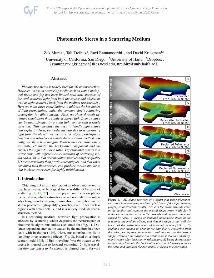
Figure 1. 3D shape recovery of a squirt gun using photomet-

ric stereo in a scattering medium. [Left] one of the input images,

[Right] reconstruction results. Err Z is the mean absolute error

in the heights and captures the overall shape error, while Err N

is the mean angular error in the normals and captures the error

caused by noise. a) Result of standard photometric stereo in air.

It ignores the medium effects, and thus the shape is not well de-

fined. b) Reconstruction result of a recent method [32]. c) By

applying our method to account for blur due to scattering from

the object, we improve the previous result and recover the correct

shape. However the surface still exhibits noise due to a small dy-

namic range after backscatter subtraction. d) Using fluorescence

to optically eliminate the backscatter prior to deblurring reduces

the noise and produces the best result. e) Result in clear water.

3415

scattering; 3) light traveling from the source is scattered

back towards the camera without hitting the object. Thisis known as backscatter and is an additive component thatveils the object. All these effects are distance dependentand thus depend on the object 3D surface: the property weaim to reconstruct. To handle this we introduce the small

surface variations approximation for the object (Sec. 3),that assumes surface changes are small relative to the dis-tance from the object (that is assumed to be known). Thisassumption removes the dependence on the unknown sur-face heights Z, but unlike the common distant light/cameraapproximations, it still allows for dependencies on spatiallocations X and Y . One important consequence of this isthe ability to model anisotropic light sources, which is notpossible for distant lights.

Forward scatter was previously compensated for itera-tively for both pathways (light to object and object to cam-era) simultaneously [21]. We analyze the paths separately.The resulting algorithm is simpler, requires fewer imagesand yields better results. First, consider the blurring of lighttraveling to the object from the source (Fig. 2b). The pho-tometric stereo formulation assumes a point light source,illuminating from a single direction. However, if the sourceis scattered by the medium, this no longer holds: the pointlight source is spread, and the direction of light rays inci-dent on the object changes. Nonetheless, for a Lambertiansurface, illuminated from a variety of directions, we stillget a linear equation between the image intensities and thesurface normals [24]. Here, we show through simulationsin a large variety of single scattering media, that a forward-scattered light source illuminating a Lambertian surface canbe well approximated by a non-blurred light source in an ef-fective purely absorbing medium (Sec. 6). This allows formuch easier calibration in practice.

Next, we observe that the blur caused by scattering from

the object to the camera (Fig. 2c) significantly affects theshape of the surface reconstructed by photometric stereo.This important effect has been neglected in many previousworks. In general, the point-spread function (PSF) for anobject is spatially varying and dependent on the unknownscene depths. However, we demonstrate that a spatially in-variant approximation can still achieve good results, whencalibrated for the desired medium and approximate objectdistance. We estimate the PSF and use it to deconvolve theimages after backscatter has been removed (Sec. 7). Thesecorrected images are used as input to a linear photometricstereo algorithm to recover the surface normals, which arethen integrated. This results in much higher quality 3D sur-faces across varying turbidity levels.

Finally, consider the backscatter component (Fig. 2a).In a previous work (Tsiotsios et al. [32]) backscatter wascalibrated and subtracted from the input images. However,when backscatter is strong relative to the object signal, sub-tracting it after image formation leads to lack of dynamicrange and lower signal-to-noise ratios (SNR) [30] that sig-nificantly degrades deblurring and reconstruction. Here we

show that if the object fluoresces, this can be leveragedto optically remove the backscatter prior to image forma-tion (Sec. 8). Fluorescence is the re-emission of photons inwavelengths longer than the excitation light [6], and there-fore the backscatter can be eliminated by optically block-ing the excitation wavelengths and imaging only the fluo-rescence emission. This improves SNR, especially in highturbidity. This approach is feasible as many natural under-water objects such as corals and algae fluoresce naturally.

We demonstrate our method experimentally in a watertank (Sec. 10) with varying turbidity levels. Deblurring canbe used separately or combined with fluorescence imagingto significantly improve the quality of photometric stereoreconstructions, as shown in Fig. 1.

2. Previous Work

The traditional setup for photometric stereo assumes aLambertian surface, orthographic projection, distant lightsources, and a non-participating medium [34]. However,underwater light is exponentially attenuated with distance,and thus the camera and lights must be placed close to thescene for proper illumination. This means that the ortho-graphic camera model, and the distant light assumptions,are no longer valid. In addition, attenuation and scatteringby the medium need to be accounted for. These effects werepartially considered in previous works.

Near-Field Effects and Exponential Attenuation: Pho-tometric stereo in air was solved with perspective cam-eras [17, 27], nearby light sources [14], or both [4, 11].Kolagani et al. [16] uses a perspective camera, nearby lightsources and includes exponential attenuation of light in amedium. Their formulation leads to nonlinear solutions forthe normals and heights. We handle these near field effectsbut linearize the problem (Sec. 3).

Photometric Stereo with Backscatter: Narasimhan etal. [20] handles backscatter and attenuation, with the as-sumption of distant light sources and an orthographic cam-era. Tsiotsios et al. [32] extends this to nearby point sourcesand assumes the backscatter saturates close to the cameraand thus does not depend on the unknown surface height.Then, it can be calibrated and subtracted from the images.We use the method in [32] in one of our variants.

Backscatter Removal: Backscatter was previously re-moved for visibility enhancement, by structured light [7],range-gating [15], or using polarizers [29]. Nevertheless,these methods do not necessarily preserve photometric in-formation. It is sometimes possible to reduce backscatterby increasing the camera light source separation [7, 12], butthis often leads to more shadowed regions, creating prob-lems for photometric stereo.

Fluorescence Imaging: Removing scatter using fluores-cence is used in microscopy [33], where many objects ofinterest are artificially dyed to fluoresce. Hullin et al. [9]imaged objects immersed in a fluorescent liquid to recon-struct their 3D structure. It was recently shown that thefluorescence emission yields photometric stereo reconstruc-

3416

XZ

Y

D

S

backscatter

XZ

YS

X

D

forward scatter (source)

XZ

S

X

forward scatter (object)

X’

Y

X

α

α α-ω

a b c

Figure 2. A perspective camera is imaging an object point at X, with a normal N, illuminated by a point light source at S. The object is

in a scattering medium, and thus light may be scattered in the three ways shown, detailed in Sec. 3.

tions [23, 28] in air that are superior to reflectance imagesas the fluorescence emission behaves like a Lambertian sur-face due to its isotropic emission.Deblurring Forward Scatter: Zhang et al. [35] and Ne-gahdaripour et al. [21] handle blur caused by forward scat-ter using the PSF derived in [12, 18]. Their PSF dependson the unknown distances, as well as three empirical pa-rameters, and affects both the path from the light source tothe object and from the object to the camera. They itera-tively deconvolve and update the depths until a good resultis achieved. Trucco et al. [31] simplify the PSF of [12, 18]to only depend on two parameters while assuming the depthis known. Our PSF is nonparametric, independent of theunknown depths and only affects the path to the camera,which allows for a direct solution without iteration. Whilewe look at a Lambertian surface in a scattering medium, In-oshita et al. [10] and Dong et al. [3] consider the problem ofphotometric stereo in air on a surface that exhibits subsur-face scattering, which blurs the radiance across the surface.They deconvolve the images to improve the quality of thenormals recovered using linear photometric stereo. Tanakaet al. [26] also model forward scatter blur as a depth de-pendent PSF and combine it with multi (spatial) frequencyillumination to recover the appearance of a small number ofinner slices of a translucent material.

3. Overview and Assumptions

In this section we introduce the image formation model,considering each of the modes of light propagation in a sin-gle scattering medium, as shown in Fig. 2. We derive ex-pressions for each component in the following sections.

Consider a perspective camera placed at the origin, withthe image (x, y) coordinates parallel to the world’s (X,Y )axes, and the Z-axis aligned with the camera’s optical axis.Let the point X = (X,Y, Z) be the point on the object’ssurface along the line of sight of pixel x = (x, y). Let Sbe the world coordinates of a point light source, and defineD(X) = S−X as the vector from the object to the source.

We assume a single scattering medium which allows usto express the radiance Lo reflected by a surface point as thesum of two terms:

Lo(x) = Ld(x) + Ls(x) (1)

where Ld is the direct radiance from the source (Sec. 4), and

Ls is the radiance from the source which is scattered fromother directions onto X (Sec. 6 and Fig. 2b).

Next, we express the radiance arriving at the camera asthe sum of three terms:

L(x) = Lo(x)e−σ‖X‖ + Lb(x) + Lc(x) (2)

where Lo, is the light reflected by the surface point X whicharrives at the camera without undergoing scattering. Notethat it is attenuated by e−σ‖X‖ where σ is the extinctioncoefficient. Lb is composed of rays of light emitted by thesource that are scattered into x’s line of sight before hit-ting the surface (Sec. 5 and Fig. 2a). This term is knownas backscatter. Finally, Lc, is composed of rays of light re-flected by other points on the surface that are scattered intopixel x’s line of sight (Sec. 7 and Fig. 2c).

In order to write analytic expressions for these terms andderive a simple solution we make two assumptions. First,the surface is Lambertian with a spatially varying albedoρ(X). Second, we assume that surface variations in heightare small compared to object distance from the camera.We call this the small surface variations approximation andnote that it is weaker than the common distant light sourcesand orthographic projection approximations. Let Z be theaverage Z coordinate of the surface (assumed to be known).Then, the approximation claims that for every point on thesurface: |Z(X)− Z| ≪ Z, ∀X.

The approximation results in a weak perspective suchthat the projection x of X in the image plane is given by

x =

(

fX

Z, f

Y

Z

)t

; X =

(

Z

fx,

Z

fy, Z

)t

, (3)

where f is the known focal length. Note that for a givenpixel, since we know its (x, y) coordinates and the aver-age object distance Z, the world coordinates X are known.Specifically, D(X) is independent of the unknown objectheight Z but still depends on X and Y , whereas in the dis-tant light sources approximation D(X) is a constant.

Outline of Our MethodGiven an input image L we eliminate the backscatter Lb

by one of two methods. The first follows [32]: backscatterfrom each light source is measured by imaging it with noobjects in the scene, and then the measured backscatter is

3417

subtracted from the input images. In the second, backscatteris optically eliminated using fluorescence as we explain inSec. 8. Once backscatter is removed, the resulting imagesare deblurred, using a calibrated PSF, to recover Lo (Sec. 7,Eq. 18). Next we write Lo as a linear equation between theunknown surface normals, albedo and an equivalent lightsource (Sec. 6, Eq. 9), which we approximate as an effectivepoint source in a purely absorbing medium with effectiveextinction coefficient (Sec. 6, Eq. 11). With a minimumof 3 images under distinct light locations the normals canbe solved for, as in conventional photometric stereo. Thenormals are then integrated to recover a smooth surface.

4. Direct Radiance

First, consider the direct reflected radiance from a Lam-bertian surface[34]:

Ld(x) = I(X)ρ(X)

πD(X) · N , (4)

where N is the unit surface normal and D is the normalizedsource-to-object vector. The radiance on the object surfaceI(X) depends on the radiant intensity I0 of the source in

direction1 (−D):

I(X) =(

I0(

− D(X))

e−σ‖D(X)‖)

/‖D(X)‖2 . (5)

Eq. 5 accounts for nearby angularly-varying sources, expo-nential attenuation along the optical path length with extinc-tion coefficient σ, and inverse-square distance falloff.

5. Backscatter

Light is scattered as it travels through a medium. Thefraction of light scattered to each direction is determined bythe phase function P (α), where α ∈ [0, 2π] is the anglebetween the original ray direction and scattered ray, and βis the scattering coefficient.

Light which is scattered directly into the camera by themedium without reaching the object is termed backscatter

and is given by [19, 25] (Fig. 2a):

Lb(x) = β

∫ ‖X‖

0

I(rX)P (α)e−σrdr (6)

The integration variable r is the distance from the camerato the imaged object point X along the line of sight (LOS),

that is a unit direction X. The scattering angle α is given by

cos(α) = D · X (recall that D is the direction to the light)

and I(rX) is the direct radiance of the source at point rXas defined in Eq. 5.

Note that for the small surface variations approximation,X and hence the limits of the integral are known for a givenpixel. Therefore, the backscatter does not depend on theunknown height of the object and is a (different) constantfor each pixel, similar to Tsiotsios et al. [32].

1the direction is negative as we consider outgoing rays from the source.

6. Single Scattered Source Radiance

Because of the medium, light rays that are not originallypointed at an object point may be scattered and reach it fromthe entire hemisphere of directions Ω (Fig. 2b), termed for-ward scattered radiance

Ls(x) =ρ(X)

π

∫

ω∈Ω

Li(ω)(ω · N) dω . (7)

where Li(ω) is the total radiance scattered into the directionω and is given by

Li(ω) = β

∫ ∞

t=0

I(X+ tω)P (α)e−σtdt , (8)

where t is the distance from the object, and the angle α is

given by cos(α) = D(X + tω) · ω. Note that D is thedirection of the integration point to the light.

Substituting Eqs. 4,7 into Eq. 1 and rearranging yields:

Lo(X) = Ld(X) + Ls(X) =ρ(X)

πL

eq(X) · N , (9)

where

Leq(X) = I(X)D(X) +

∫

ω∈Ω

Li(ω)ω dω . (10)

Here, the direct light as well as the integrated scattered con-tributions can be thought of as an equivalent distant lightsource not in a medium, although, this equivalent sourcemay be different (in direction and magnitude) for each sur-face point, and thus is not a true distant source. Neverthe-less, Eq. 9 gives a linear equation for the unknown normalsand albedo, which can be solved for given a minimum of 3images under distinct light locations.

Unfortunately, evaluating Eq. 10 requires careful calibra-tion of the scattering parameters β, σ and P (α) which canbe difficult. Instead, we next show through simulations, thatfor a wide variety of media, Leq(X) can be approximatedas an effective point source in a purely absorbing mediumwith effective extinction coefficient. This allows for simplecalibration.

Effective Point Source Simulations

We approximate Leq(X) as:

Leq(X) ≈

κI0(

− D(X))

e−σ‖D(X)‖

‖D(X)‖2D(X) , (11)

where the effective source has the same position S and in-tensity distribution I0 as the real source, but is scaled by κ,and the effective medium has extinction coefficient σ. Notethat κ is a global brightness scale, which is the same for allthe lights, and thus does not need to be explicitly calibrated,as it cancels out in the normal estimation.

For our simulations we used an isotropic point source at adistance d from a Lambertian surface patch with an angle φ

3418

a b% Error % Error

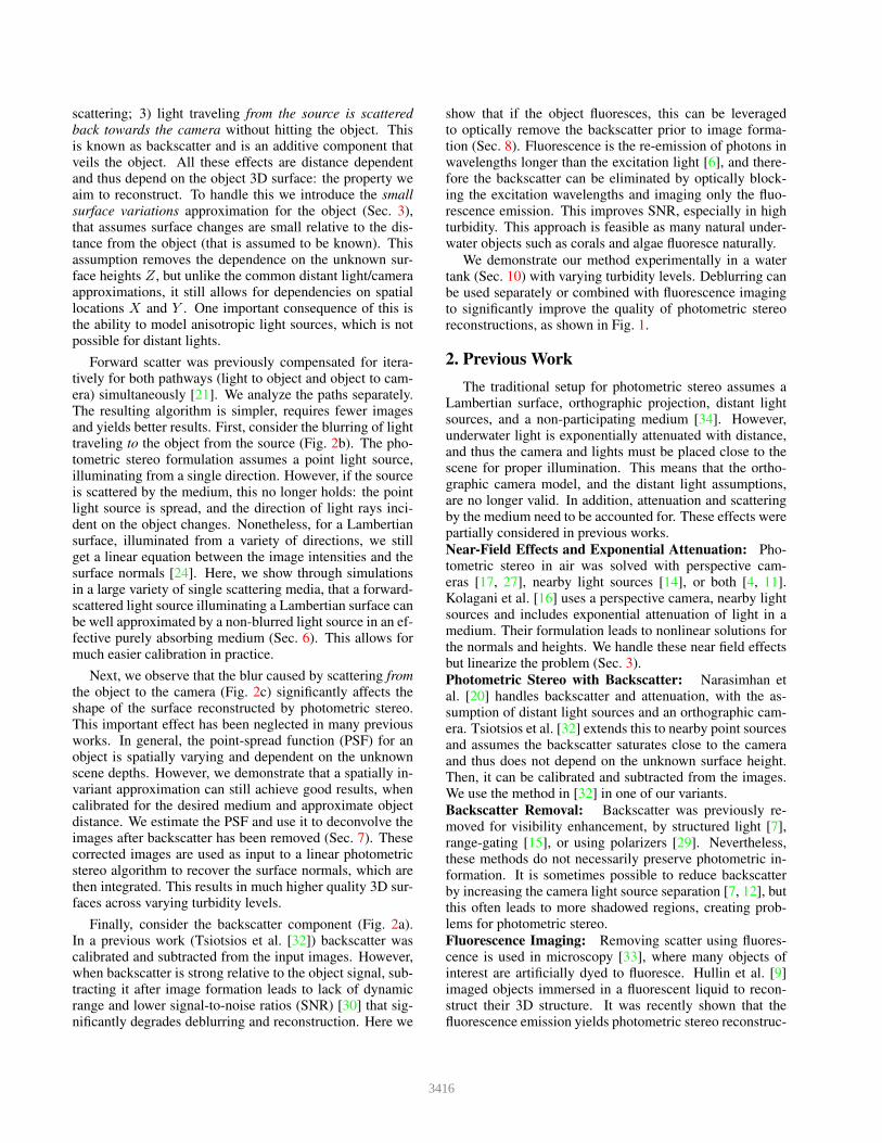
Figure 3. a) The relative error between Lo(d, φ) and Lo(d, φ) for

g = 0.8 and β = 0.0026. Note that the spike only reaches 3% and

is located at φ = 90 where Lo = 0 due to shadowing. φ near 90

and above is not usually relevant for photometric stereo. b) The

mean relative error between Lo and Lo for β ∈ [0, 0.005]mm−1

and g ∈ [0, 0.9]. The approximation errors are small.

between the surface normal and light direction. For the scat-tering function, we used the common Henyey-Greensteinphase function [8] that has a single parameter of the mediumg ∈ [−1, 1]. In water, g is usually between 0.7− 0.9 [19].

We compute Lo(d, φ) for d ∈ [200, 600]mm, φ ∈ [0, π],for a variety of media given by β ∈ [0, 0.005]mm−1 andg ∈ [0, 0.9]. Note that we choose I0 such that Lo(200, 0) isnormalized to 1. To reduce the number of parameters we setσ = β, which does not influence the analysis2. For each pa-rameter pair g, β we compute the approximation parametersκ and σ by minimizing:

minκ,σ

∑

d,φ

|Lo(d, φ)− Lo(d, φ)|2 . (12)

As an example, Fig. 3a depicts the relative error,

RE(d, φ) = |Lo(d, φ)−Lo(d, φ)|, for g = 0.8, β = 0.0026,that fit our setup. Figure 3b depicts the mean relative er-ror (MRE) for a range of values β ∈ [0, .005]mm−1 andg ∈ [0, .9], where the mean is taken over d and φ. The MREwas less than 2% across all medium conditions, justifyingour approximation.

7. Single Scatter Object Blur

Similar to the light source blur, radiance from the objectis also blurred while it propagates to the camera (Fig. 2c).As we demonstrate, this effect deteriorates the performanceof photometric stereo, although it has been neglected in pre-vious works [25].

The contribution of object blur to the pixel intensity iscomputed by integrating light scattered into the LOS of Xfrom all other points on the surface:

Lc(x) = β

∫ ‖X‖

r=0

∫

ω∈Ω

Lo(X′)P (α)e−σ(t+r) dωdr.

(13)Here r is the distance along the LOS, X′ is the object sur-face point intersected by the ray starting at point rX in di-rection ω. Its radiance is Lo(X

′) and its distance to the

scatter point in the LOS is given by t = ‖rX − X′‖ with

scattering angle cosα = ω · (−X).

2In general β ≤ σ, but since β purely scales Ls, a smaller value of

beta would make Lo closer to Ld and thus L0 would be an even better fitthan we calculated.

We now show that Lo can be recovered fromLoe

−σ‖X‖ + Lc by deconvolution with a constant PSF.

Deblurring Object ScatterFirst we rewrite Eq. 13 to integrate over the area of the

object surface dA = dω · t2/ cos θ instead of solid angledω, where t is the distance from X

′ to the scattering event,and θ is the angle between the normal at X′ and the ray oflight before scattering. Eq. 13 now becomes

Lc(x) = β

∫

X′

Lo(X′)

∫ ‖X‖

0

P (α)e−σ(t+r) cos θ

t2dr dA.

(14)Now we define the scattering kernel

K(X,X′) = δ(X−X′)e−σ‖X‖ +

β

∫ ‖X‖

0

P (α)e−σ(t+r) cos θ

t2dr, (15)

where δ(X−X′) is the Dirac delta function. Now,

Lo(x)e−σ‖X‖ +Lc(x) =

∫

X′

K(X,X′)Lo(X′) dA(X′) .

(16)In general, the kernel K, depends on X, X′ and the un-

known normals N′. For an orthographic camera viewing aplane at constant depth, K is shift invariant and Eq. 16 canbe written as a convolution with a PSF. Motivated by this,we found empirically that for a given Z it is approximatelyshift invariant (and rotationally symmetric).

Denoting the PSF as h, we get

Lo(x)e−σ‖X‖ + Lc(x) ≈ h ∗ Lo . (17)

We emphasize here that we have shown that under a sin-gle scattering model, the forward scatter from the object canbe written as an integral transform with kernel K. This jus-tifies approximating the forward scattering as a PSF whichis not obvious in the form of Eq. 13.

We solve Eq. 17 by writing the image as a column vectorand representing the convolution as a matrix operation

L− Lb = HLo (18)

where we have substituted the backscatter compensated im-age L − Lb for Loe

−σ‖X‖ + Lc, and H is the matrix rep-resentation of h. Here H is a large nonsparse matrix andthus storing it in memory and directly inverting it is infea-sible. Instead we solve the linear system of Eq. 18 usingconjugate gradient descent. This requires only the matrixvector operation which can be computed as a convolutionand implemented using a Fast Fourier Transform (FFT).

8. Backscatter Removal Using Fluorescence

While we are able to subtract the backscatter compo-nent, it is an additive component that effectively reduces

3419

reflectance( fluorescence(a

b c

reflectance( fluorescence(

backsca.er(

(((((reflectance(

backsca.er(

((fluorescence( (((((

d e

deblurred(reflectance( deblurred((fluorescence(

Figure 4. a) Backscatter is caused by light that is scattered into the

camera by a medium, before it reaches the object and has the same

color as the illumination. Thus, the barrier filter used to block

fluorescence excitation also blocks backscatter, while imaging the

signal from the object. We use this property to remove backscatter

in input images. b) Photometric stereo reconstruction of a fluores-

cent sphere using backscatter subtracted reflectance images. One

of the input images is shown on the left, with visible noise and blur.

Blur in the input images flattens the reconstruction. c) Looking

at fluorescence images as an input, the backscatter is eliminated

while maintaining a higher SNR. However the blur still flattens the

reconstruction. d) Deblurring the backscatter subtracted images

recovers the general shape but suffers from noise as seen by the

spiky surface. e) Deblurring the fluorescence results in the correct

shape with much less noise.

the dynamic range of the signal from the object, degradesthe image quality and reduces SNR [30]. As such it isbeneficial to optically remove it when imaging. Here, weuse the observation that for fluorescence images taken withnon-overlapping excitation and emission filters, there is nobackscatter in the image (Fig. 4a). In fluorescence imaging,the signal of interest is composed of wavelengths that arelonger than that of the illumination, and a barrier filter onthe camera is used to block the reflected light. The backscat-ter is composed of light scattered by the medium before itreaches the object. Thus, the backscatter has the same spec-tral distribution as the light source, which is blocked by thebarrier filter on the camera. This insight enables imagingwithout loss of dynamic range even in highly turbid me-dia. Compared to a backscatter subtracted reflectance im-age, a fluorescence image has less noise (Fig. 4b,c). Thisdifference becomes even more apparent after deconvolution(Fig. 4d,e).

In addition, in [23, 28] it was shown that the fluorescenceemission acts as a Lambertian surface in photometric recon-structions. Thus, imaging fluorescence has an additionaladvantage as it relaxes the need for a Lambertian surface.

In the development of our algorithm we assumed a sin-gle set of medium parameters β, σ and P (α). Howeverthese quantities are in general wavelength dependent. In re-flectance imaging, the wavelength of the light is the same onboth pathways: light to object, and object to camera. How-

LED’sCamera

Ob

ject

LED

BackscatterCamera

Object

Top ViewFront View

Figure 5. [Left] Our experimental setup consists of a camera

looking through a glass port into a tank. [Right] 8 LEDs are

mounted inside the tank around the camera port illuminating the

object placed at the back of the tank.

ever, in fluorescence imaging they are different. Neverthe-less, the only parameters that require calibration in our so-lution are the effective extinction coefficient σ and the PSF.The parameter σ is estimated for the excitation wavelengthand the PSF is estimated for the emission wavelength, andas such we do not need to calibrate any extra parameters inthe case of fluorescence imaging.

9. Implementation

9.1. Experimental Setup

Our setup is shown in Fig. 5. We used a Canon 1D cam-era with a 28mm lens placed 2cm away from a 10 gallonglass aquarium. All sides except the front (where the cam-era looks in) were painted black to reduce reflection. Inaddition, a black panel was suspended just below the sur-face of the water to remove reflection from the air-waterinterface. The objects were placed at an average distance of40cm from the front of the tank. For point illumination weused Cree XML - RGBW Star LEDs. The LEDs were waterproofed by coating the electrical terminals with epoxy. Re-flection images were taken under white illumination whilefluorescent images were taken under blue illumination witha Tiffen #12 emission filter on the camera. We used tapwater, and the turbidity was increased using a mixture ofwhole milk and grape juice (milk is nearly purely scatter-ing, while grape juice is nearly purely absorbing and thusby mixing them we can achieve a variety of scattering con-ditions [19]). The LEDs were mounted inside the tank ona square around the camera, four on the corners and fouron the edges. Their positions were measured. Images wereacquired in Raw mode which is linear and the normal inte-gration was done using the method of [1].

9.2. Geometric and Radiometric Calibration

Images of a checkerboard (in clear water) were usedto calibrate the intrinsic camera parameters (implicitly ac-counting for refraction) [2]. The location of each light was

3420

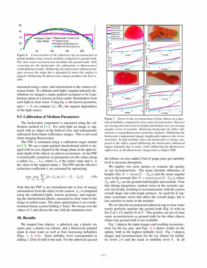
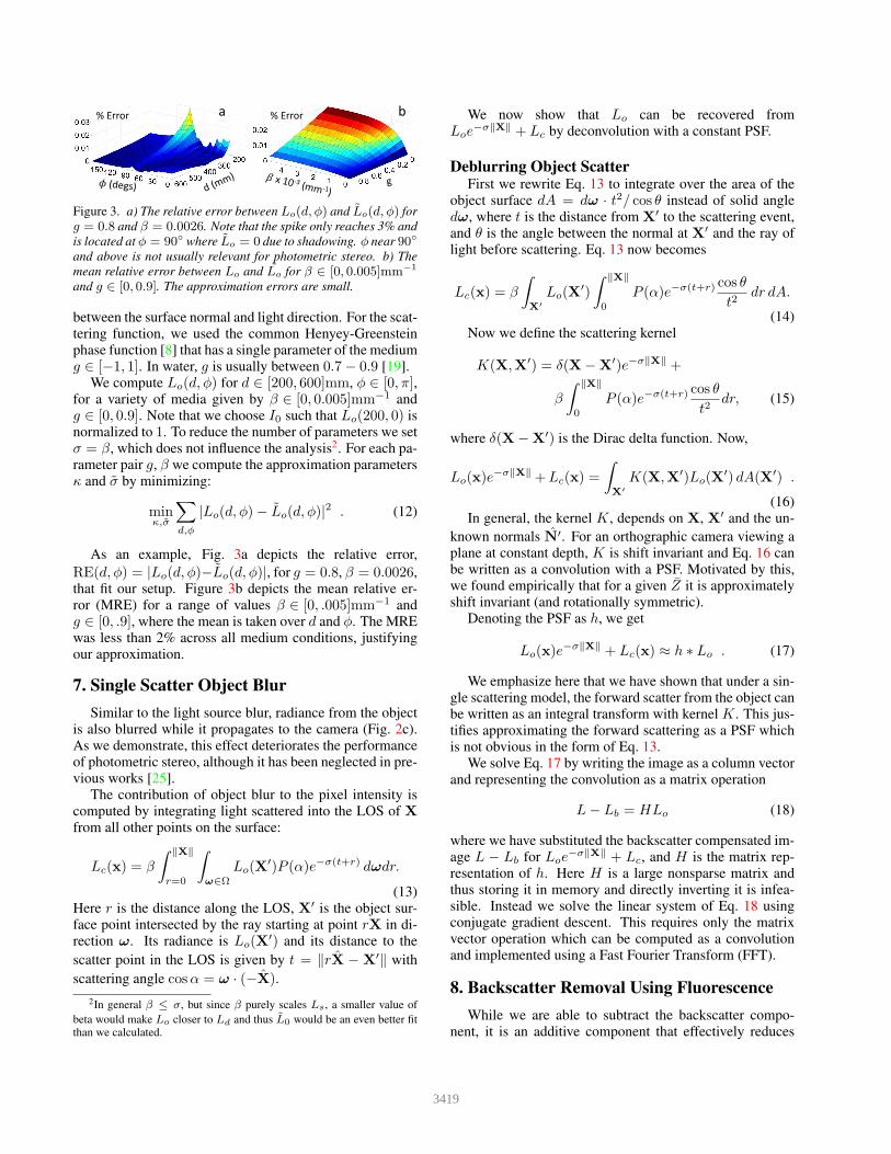
Figure 6. Cross-sections of the spherical cap reconstruction in

turbid medium using various methods compared to ground truth.

The clear water reconstruction resembles the ground truth. Only

correcting for the backscatter (by subtraction or fluorescence)

yields flattened results. Deblurring the backscatter subtracted im-

ages recovers the shape but is degraded by noise (the surface is

jagged). Deblurring the fluorescence images produces the best re-

sults.

measured using a ruler, and transformed to the camera ref-erence frame. To calibrate each light’s angular intensity dis-tribution we imaged a matte painted (assumed to be Lam-bertian) plane at a known position under illumination fromeach light in clear water. Using Eq. 4, the known geometry,

and σ = 0, we compute I0(−D), the angular dependenceof the light source.

9.3. Calibration of Medium Parameters

The backscatter component is measured using the cal-ibration method of [32]. For each light an image is cap-tured with no object in the field-of-view and subsequentlysubtracted from future reflectance images. This is not usedwhen imaging fluorescence.

The PSF is estimated using a calibration target similarto [13]. We use a matte painted checkerboard which is im-aged with its axis aligned to the image plane at the approxi-mate depth of the objects we plan to reconstruct. As the PSFis rotationally symmetric its parameters are the values alonga radius [h0, ..., hs], where h0 is the center value and hs isthe value on the support radius s. The PSF and the effectiveextinction coefficient σ are estimated by optimizing

minσ

minh0...hs

∑

x

‖h ∗ Lo(x, σ)− (L− Lb)‖ (19)

Note that the PSF is not normalized due to loss of energy(attenuation) from the object to the camera. Lo is computedusing the calibrated lights, known geometry, and register-ing the checkerboard albedo, measured in clear water to theimage in turbid water. The inner optimization is an overde-termined linear system holding σ fixed. We sweep over thevalues of σ and choose the one with the minimum error.

10. Results

We imaged four objects: a spherical cap, a plastic toysquirt gun, a plastic toy lobster, and a fluorescent paintedmask in clear water as well as four increasing turbidities(Figs. 1, 4, 6-8). Each turbidity level corresponded toadding 1.25ml of milk to the tank. For the spherical cap and

Backscatter subtracted

Fluorescence

DeblurredReflectance

DeblurredFluorescence

Figure 7. Errors in the reconstructions of four objects as a func-

tion of turbidity, compared to clear water reconstruction. Top rows

are average percent errors in heights and bottom rows are average

angular errors in normals. Removing backscatter by either sub-

traction or using fluorescence performs similarly. Deblurring the

backscatter compensated images significantly improves the recon-

structions. In high turbidity where the backscatter is strong com-

pared to the object signal deblurring the backscatter subtracted

images degrades due to noise, while deblurring the fluorescence

suffers less, as the fluorescence images have a higher SNR.

the lobster, we also added 15ml of grape juice per turbiditylevel to increase absorption.

We employ two error metrics to evaluate the qualityof our reconstructions: The mean absolute difference inheights (Err Z = mean(Z − Zgt)) and the mean angularerror in the normals (Err N = mean(acos(N ·Ngt)), whereZgt and Ngt are the ground truth heights and normals. Notethat during integration, random noise in the normals can-cels out locally, resulting in reconstructions with the correctoverall shape, but with rough surfaces. As such Err Z cap-tures systematic errors that affect the overall shape, but isless sensitive to noise in the normals.

We see that the reconstructed spherical cap in clear waternearly perfectly matches the ground truth (Fig. 6) with anErr Z of 1.4% and Err N of 3. This justifies our use of clearwater reconstructions as ground truth for the other objectswhere true ground truth is not available.

Fig. 1 depicts the input images and resulting reconstruc-tions for the toy gun, and Figs. 4, 6 depict results on thesphere, both in the highest turbidity level. Fig. 8 depictsimages and reconstructions for the toy lobster for turbid-ity levels 2-4 and the mask in turbidity level 4. In all

3421

Ba

cksc

att

er

Co

mp

en

sate

dD

eb

lurr

ed

Flu

ore

sce

nce

Flu

ore

sce

nce

Re

fle

cta

nce

Re

fle

cta

nce

Un

corr

ect

ed

Increasing Turbidity

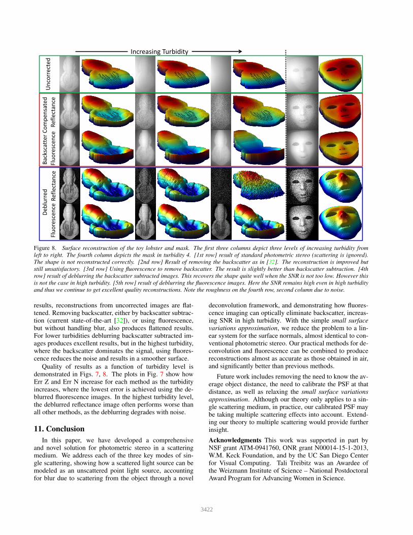
Figure 8. Surface reconstruction of the toy lobster and mask. The first three columns depict three levels of increasing turbidity from

left to right. The fourth column depicts the mask in turbidity 4. [1st row] result of standard photometric stereo (scattering is ignored).

The shape is not reconstructed correctly. [2nd row] Result of removing the backscatter as in [32]. The reconstruction is improved but

still unsatisfactory. [3rd row] Using fluorescence to remove backscatter. The result is slightly better than backscatter subtraction. [4th

row] result of deblurring the backscatter subtracted images. This recovers the shape quite well when the SNR is not too low. However this

is not the case in high turbidity. [5th row] result of deblurring the fluorescence images. Here the SNR remains high even in high turbidity

and thus we continue to get excellent quality reconstructions. Note the roughness on the fourth row, second column due to noise.

results, reconstructions from uncorrected images are flat-tened. Removing backscatter, either by backscatter subtrac-tion (current state-of-the-art [32]), or using fluorescence,but without handling blur, also produces flattened results.For lower turbidities deblurring backscatter subtracted im-ages produces excellent results, but in the highest turbidity,where the backscatter dominates the signal, using fluores-cence reduces the noise and results in a smoother surface.

Quality of results as a function of turbidity level isdemonstrated in Figs. 7, 8. The plots in Fig. 7 show howErr Z and Err N increase for each method as the turbidityincreases, where the lowest error is achieved using the de-blurred fluorescence images. In the highest turbidity level,the deblurred reflectance image often performs worse thanall other methods, as the deblurring degrades with noise.

11. Conclusion

In this paper, we have developed a comprehensiveand novel solution for photometric stereo in a scatteringmedium. We address each of the three key modes of sin-gle scattering, showing how a scattered light source can bemodeled as an unscattered point light source, accountingfor blur due to scattering from the object through a novel

deconvolution framework, and demonstrating how fluores-cence imaging can optically eliminate backscatter, increas-ing SNR in high turbidity. With the simple small surface

variations approximation, we reduce the problem to a lin-ear system for the surface normals, almost identical to con-ventional photometric stereo. Our practical methods for de-convolution and fluorescence can be combined to producereconstructions almost as accurate as those obtained in air,and significantly better than previous methods.

Future work includes removing the need to know the av-erage object distance, the need to calibrate the PSF at thatdistance, as well as relaxing the small surface variations

approximation. Although our theory only applies to a sin-gle scattering medium, in practice, our calibrated PSF maybe taking multiple scattering effects into account. Extend-ing our theory to multiple scattering would provide furtherinsight.

Acknowledgments This work was supported in part byNSF grant ATM-0941760, ONR grant N00014-15-1-2013,W.M. Keck Foundation, and by the UC San Diego Centerfor Visual Computing. Tali Treibitz was an Awardee ofthe Weizmann Institute of Science – National PostdoctoralAward Program for Advancing Women in Science.

3422

References

[1] A. Agrawal, R. Raskar, and R. Chellappa. What is the range

of surface reconstructions from a gradient field? In Proc.

ECCV, pages 578–591. Springer, 2006. 6

[2] J. Y. Bouguet. Camera calibration toolbox for matlab.

vision.caltech.edu/bouguetj/calib_doc. 6

[3] B. Dong, K. D. Moore, W. Zhang, and P. Peers. Scattering

parameters and surface normals from homogeneous translu-

cent materials using photometric stereo. In Proc. IEEE

CVPR, pages 2299–2306, 2014. 3

[4] M. Galo and C. L. Tozzi. Surface reconstruction using mul-

tiple light sources and perspective projection. In Proc. IEEE

ICIP, volume 1, pages 309–312, 1996. 2

[5] N. Gracias, P. Ridao, R. Garcia, J. Escartin, M. L’Hour,

F. Cibecchini, R. Campos, M. Carreras, D. Ribas, N. Palom-

eras, et al. Mapping the moon: Using a lightweight auv to

survey the site of the 17th century ship la lune. In Proc.

MTS/IEEE OCEANS. IEEE, 2013. 1

[6] G. Guilbault. Practical fluorescence, volume 3. CRC, 1990.

2

[7] M. Gupta, S. Narasimhan, and Y. Schechner. On controlling

light transport in poor visibility environments. In Proc. IEEE

CVPR, 2008. 2

[8] L. G. Henyey and J. L. Greenstein. Diffuse radiation in the

galaxy. The Astrophysical Journal, 93:70–83, 1941. 5

[9] M. Hullin, M. Fuchs, I. Ihrke, H. Seidel, and H. Lensch. Flu-

orescent immersion range scanning. ACM Transactions on

Graphics (TOG), 27(3):87–87, 2008. 2

[10] C. Inoshita, Y. Mukaigawa, Y. Matsushita, and Y. Yagi. Sur-

face normal deconvolution: Photometric stereo for optically

thick translucent objects. In Proc. ECCV, pages 346–359.

Springer, 2014. 3

[11] Y. Iwahori, H. Sugie, and N. Ishii. Reconstructing shape

from shading images under point light source illumination.

In Proc. IEEE ICPR, volume 1, pages 83–87, 1990. 2

[12] J. S. Jaffe. Computer modeling and the design of optimal

underwater imaging systems. IEEE J. Oceanic Engineering,

15(2):101–111, 1990. 2, 3

[13] N. Joshi, R. Szeliski, and D. Kriegman. PSF estimation us-

ing sharp edge prediction. In Proc. IEEE CVPR, pages 1–8.

IEEE, 2008. 7

[14] B. Kim and P. Burger. Depth and shape from shading using

the photometric stereo method. CVGIP: Image Understand-

ing, 54(3):416–427, 1991. 2

[15] D. Kocak, F. Dalgleish, F. Caimi, and Y. Schechner. A focus

on recent developments and trends in underwater imaging.

Marine Technology Society Journal, 42(1):52–67, 2008. 1, 2

[16] N. Kolagani, J. Fox, and D. Blidberg. Photometric stereo

using point light sources. In Proc. IEEE Int. Conf. Robotics

and Automation, pages 1759–1764, 1992. 1, 2

[17] K. M. Lee, C. J. Kuo, et al. Shape from photometric ratio and

stereo. J. Vis. Comm. & Image Rep., 7(2):155–162, 1996. 2

[18] B. McGlamery. A computer model for underwater camera

systems. In Ocean Optics VI, pages 221–231. International

Society for Optics and Photonics, 1980. 3

[19] S. G. Narasimhan, M. Gupta, C. Donner, R. Ramamoorthi,

S. K. Nayar, and H. W. Jensen. Acquiring scattering prop-

erties of participating media by dilution. ACM Transactions

on Graphics (TOG), 25(3):1003–1012, 2006. 4, 5, 6

[20] S. G. Narasimhan, S. K. Nayar, B. Sun, and S. J. Koppal.

Structured light in scattering media. In Proc. IEEE ICCV,

pages 420–427, 2005. 2

[21] S. Negahdaripour, H. Zhang, and X. Han. Investigation of

photometric stereo method for 3-D shape recovery from un-

derwater imagery. In Proc. MTS/IEEE OCEANS, volume 2,

pages 1010–1017, 2002. 2, 3

[22] R. Pintus, S. Podda, and M. Vanzi. An automatic alignment

procedure for a four-source photometric stereo technique ap-

plied to scanning electron microscopy. IEEE Trans, Instru-

mentation and Measurement, 57(5):989–996, 2008. 1

[23] I. Sato, T. Okabe, and Y. Sato. Bispectral photometric stereo

based on fluorescence. In Proc. IEEE CVPR, 2012. 3, 6

[24] A. Shashua. Geometry and photometry in 3D visual recog-

nition. PhD thesis, Massachusetts Institute of Technology,

1992. 2

[25] B. Sun, R. Ramamoorthi, S. G. Narasimhan, and S. K. Na-

yar. A practical analytic single scattering model for real time

rendering. ACM Transactions on Graphics (TOG), 24:1040–

1049, 2005. 1, 4, 5

[26] K. Tanaka, Y. Mukaigawa, H. Kubo, Y. Matsushita, and

Y. Yagi. Recovering inner slices of translucent objects by

multi-frequency illumination. In Proceedings of the IEEE

Conference on Computer Vision and Pattern Recognition,

pages 5464–5472, 2015. 3

[27] A. Tankus and N. Kiryati. Photometric stereo under perspec-

tive projection. In Proc. IEEE ICCV, 2005. 2

[28] T. Treibitz, Z. Murez, B. G. Mitchell, and D. Kriegman.

Shape from fluorescence. In Proc. ECCV, 2012. 3, 6

[29] T. Treibitz and Y. Y. Schechner. Active polarization descat-

tering. IEEE Trans. PAMI, 31:385–399, 2009. 2

[30] T. Treibitz and Y. Y. Schechner. Resolution loss without

imaging blur. JOSA A, 29(8):1516–1528, 2012. 2, 6

[31] E. Trucco and A. T. Olmos-Antillon. Self-tuning underwater

image restoration. IEEE J. Oceanic Engineering, 31(2):511–

519, 2006. 3

[32] C. Tsiotsios, M. E. Angelopoulou, T.-K. Kim, and A. J. Davi-

son. Backscatter compensated photometric stereo with 3

sources. In Proc. IEEE CVPR, pages 2259–2266, 2014. 1,

2, 3, 4, 7, 8

[33] V. V. Tuchin and V. Tuchin. Tissue optics: light scattering

methods and instruments for medical diagnosis, volume 13.

SPIE press Bellingham, 2007. 2

[34] R. Woodham. Photometric method for determining surface

orientation from multiple images. Opt. Eng., 19(1):139–144,

January 1980. 2, 4

[35] S. Zhang and S. Negahdaripour. 3-D shape recovery of pla-

nar and curved surfaces from shading cues in underwater im-

ages. IEEE J. Oceanic Engineering, 27(1):100–116, 2002. 3

3423