Rochester Institute of TechnologyRIT Scholar Works

Theses Thesis/Dissertation Collections

5-1-1984

Photometric processing and interpretation ofratioed imagery by multivariate discriminantanalysis for separation of geological typesDonald Marsh

Follow this and additional works at: http://scholarworks.rit.edu/theses

This Thesis is brought to you for free and open access by the Thesis/Dissertation Collections at RIT Scholar Works. It has been accepted for inclusionin Theses by an authorized administrator of RIT Scholar Works. For more information, please contact ritscholarworks@rit.edu.

Recommended CitationMarsh, Donald, "Photometric processing and interpretation of ratioed imagery by multivariate discriminant analysis for separation ofgeological types" (1984). Thesis. Rochester Institute of Technology. Accessed from

PHOTOMETRIC PROCESSING AND INTERPRETATION OF RATIOEDIMAGER1

BY MULTIVARIATE DISCRIMINANT ANALYSIS FOR SEPARATION OF

GEOLOGICAL TYPES

Donald Jay Marsh

Apri 1,1984

PHOTOMETR I C PROCESS I NG AND I NTERPRETAT ION OF RAT I OED H'lAGER'(

BY MULTIVARIATE 01 SCRIMINANT ANALYSI S FOR SEPARATI (It...J elF

GEOLOGICAL TYPES

by

Dona 1d J a<.Y fvla r sh

A thesis submitted in partial fulfil lm~nt

of the requirements for the degree of

Bachelor of Science i n the School of

Photographic Arts and SCiences in the

College of Graphic Arts and Photograp~/

A thesis submi tted in partial fulfil lm~nt

of the requirements for the degree of

Bachelor of Science i n the School of

Photographic Arts and SCiences in the

College of Graphic Arts and Photograp~/

of the Rochester Institute of Tfchnology

:::ignat'Jr-e of the Authc,r .Imaging and PhotographicSc , e nc e

Ceortified by ..........•...........•.•..•......••...Th e s i: Ad\1 i ':·or

THESIS RELEASE PERMISSION FORM

ROCHESTER INSTITUTE OF TECHNOLOGY

COLLEGE OF GRAPHIC ARTS AND PHOTOGRAPHY

Title of Thesis: Photometric Processing and Interpretatio~ of

Ratioed Imagery by Multivariate Discriminant AnaJy~is for

Separation of Geological Types.

I, Donald Jay Marsh, herebY grant permission to Wal lace

Memorial Library, of R.I.T. to reproduce my thesis in whol~ or

in part. Any reproduction will not be for commercial use of

Separation of Geological Types.

I, Donald Jay Marsh, herebY grant permission to Wal lace

Memorial Library, of R.I.T. to reproduce my thesis in whol~ or

in part. Any reproduction will not be for commercial use of

prof i t.

PHOTOMETRIC PROCESSING AND INTERPRETATION OF RATIOED IMAGERY

BY MULIVARIATE DISCRIMINANT ANALYSIS FOR SEPARATION OF

GEOLOGICAL TYPES

by

Donald Jay Marsh

Submitted to the Imaging and Photographic

Science Division in partial -fulfillment

of the requirements for the Bachelor of Science

degree at the Rochester Institute of Technology

ASTRACT

A study has investigated the ability of ratioec

information from Landsat 2 Mul t i spec tral imagery, to

discriminate geological features through the application of

photometric processing techniques. United StatesGeologic:.1

survey maps corresponding to the areas investigated have been

used in correlation with ratioed imagery to identify predict

and confirm geological features on the basis of resulting

dens i tome tr i c information. A multivariate, discriminant

analysis of rock type, exposure data has enabled the

fabrication of the final, optimized ratio image. The

optimisation process used to predict geological types involved

a priority structure that found the spectral bands with the

highest discriminatory power and the least correlation and

i i i

then predicted contrast values for the positive and negative

masks. Lab test imagery of several rock samples provided

imputus for further investigation from the chosen orbital

imaging system, the Landsat Satellite series.

i v

ACKNOWLEDGEMENTS

Completion of this project was made possible by the

technical assistance and support of many persons:

Dr. John Schott for his technical support and assistance in

getting the project off the ground and continually providing

new i deas.

The R.I.T., Rochester and National branch of the Society of

Photographic Scientists and Engineers for their many

conferences in which numerious ideas have given the author

deep insight into new and inovative concepts.

The Imaging Science Faculty at R.I.T., my family and friends

for their mental and physical support, notably my father, who

time and time again kept me striving for my personal best.

DEDICATION

The author would like to dedicate this work to the

memory of John Cobb. The 1 ife of Mr. Cobb has made a profound

impact on the aspirations and accomplishments of the author.

With his death, a world of possibilities and personal dreams

that seemed impossible, became reality. It is to his living

memory that I present this work.

v I

TABLE OF CONTENTS

Page No ,

Introduction 1

Exper i men tal 24

1 Test Imagery 24

2 Mi crodens i tome ter Configuration 26

3 Landsat Imagery 27

4 Discriminant Analysis 2'?

5 Contrast Calculation 31

6 Production of Ratio Image 31

7 Analysis of Ratioed Imagery 32

Resul ts 34

Discussion of Results 47

Cone 1 us i ons 58

References '3

append i c i es 6 3

Vita 73

v i i

LIST OF TABLES

Page No.

i . Two Factorial Design Table. 21

ii . One Factor Design Table. 22

iii . Analysis of Variance Table

for Two-Way Model 28

iv . Analysis of Variance Table for

One-Way Model 32

RESULTS SECTION

1 . Two-Way Analysis of Variance

Resul ts 34

2 . Discriminant Function

Coefficients 35 & 36

3 . Correlation Results 37

4 . Classification of Known Geologic

Types

5 . Contrast Calculation Results

6 . Unknown Classification

7 . Mean Spectral Exposure Values for

Geologic Types of Original MSS

Imagery 43

3 . One-Way Analysis of Variance

Resul ts 44

9 . Resultant Densities of Ground

sites for the Ratio Mask 4*

oo &ii-i

40

41 & 42

VIII

LIST OF FIGURES

Page No.

1. Factors Relating Film Exposure to

Ground Reflectance. 2

2. Photographic Ratio Mask Fabrication. 3

3. Energy Sources and Atmospheric

Tr ansm i t tance ?

4. Low Correlation/ High Correlation

Spectral Exposure Plots. 18

5. Frequency of Occurance vs Exposure

value. 20

6. Imaged Spectra Using 2178 and

Several Filters 25

I n troduc t i on

Progress in Remote Sensing since the early 1 950'

s has

utilized multiple data acquisition and analysis techniques.

[1] The so-called"multi"

concept used in remote sensing has

several advantages and limitations which are a function of the

intended use of the resultant information. Imagery of the

earth, used for the collection of Environmental Resource Data

has taken these problems and assets into account.

Remote Sensing is concerned with the recording of

electromagnetic radiation onto an imaging system. Sensing of

the earth from above the ground can be accomplished by some

imaging systems that view features in different parts of the

spectrum simultaneously. This has been refered to as

mul t i spec tral or multi band imaging. Given a specific

composition of a ground feature, the energy reflecting +rom

that element is a function of many molecular characteristics

of the feature. The spectral reflectance of the body results

in its own unique spectral signature and is in some way .*

function of the signal produced by the electromagnetic sensor.

Mul t i spec tral photography uses this natural phenomenon to its

advantage and records information separately so the soectral

signatures can be identified from one another. Manifested

differences in the spectral reflectance between features

appear as signal differences on the ensuing image and can be

used to differentiate those featu res ,

Skylight

' ' Camera

(51 Exposure = aR + (J

(1) Incident radiation a

(with attenuation factor)

(3) Reflected energy aR

(2) Terrain element of reflectance R

"^

Figure 1. Factors Relating Film Exposure to

Ground Reflectance.

Much recent information has been dedicated to digital

imagery because of the speed of calculation, analysis and

evaluation. A many-fold increase in efficiency of handling

large amounts of data has been realized. The discipline o*

mu 1 t i spec tral image analysis has seen the capability of ijta

transformation take a quantum leap since the early nineteen

sixties. Simple transformations such as the ratio of picture

elements (pixels) from two images is quite commonplace.

Numerical pixel data is highly informative and produces high

quality results with a minimum of loss in the s -stem.

Limitations imposed by the digital process include space,

time, expensive equipment and high cost. It is possibl

however to emulate the superior "digitalprocess"

through

photographic processes. Work related to this field has

developed before computers became increasingly efficient and

substantial techniques have been developed to separate and

extract spectral reflectivity variations and other optical and

ground-atmosphere interaction effects C23 .

Ratioed images can be used to enhance the

discrimination of ground features as well as making

quantitative analysis of the spectral reflectance of the

feature. Digital ratioed images are generated by dividing

pixel values in one mu 1 t i spec tral band by the corresponding

values in another band. Photographic ratio images are made by

superimposing negative and positive contrast images of two

spectral regions.

BAND 1

BAND 2

ORIGIONAL MSS

SCENE

POSITIVE

CONTRAST

NEGATIVE

.A.

CONTRAST

COPY MASK

OVER

LAY

FINAL

RATIO

IMAGE

Figure 2. Photographic Ratio Mask

Produc t i on .

In a matrix (x,y), the ratio of the signals of the two bands

i and j can be written;

r( i, j)

=

S<x,y, i)

( e q n 1 )

S<x,y, j)

The ability of ratioed images to negate various

extranious multiplicative factors that effect photographic

radiometric data as well as sensor data has been established

by many authors in recient years [33. Spectral ratios negate

mul i tp 1 i cat i ve factors within the sensor data that act equally

in all wavelengths of analysis. Differential illumination

caused by changes in the atmosphere or topographical effects

across a scene are negated. In addition, mu 1 t i spec tral ratios

provide a good estimate of the average scene brightness and

eliminates confusion between reflected electromagnetic

radiation and other variations. Topographically induced

brightness variations of individual spectral bands has been a

problem that has limited the success of many studies of

reflected radiation since the early 1960's C43. It is assumed

that the modulation of the brightness of a scene due to

topography is generally independent of material properties and

wavelength spectra, therefore mul t i spec tral band ratios can be

used to discriminate material properties. Rat icing eliminates

relief shading and it has been suggested that the stereoscopic

ef-f

,;t could be used to enhance the three dimensional context

of spectral patterns so as to more fully see the three

dimensional representation of the spectral components [5,63.

In theory each type of ground feature has a specific

spectral signature which can be identified using appropriate

spectral sensing equipment. In reality spectral reflectance

curves of any given feature are affected by many things

contributing to the degradation and blurring of the final

product. These signatures may even vary within a certain

species, from one site to another. A few factors influencing

soil reflectance, are moisture content, soil texture,

(proportion of sand and clay) surface roughness, the presence

of iron oxide, and organic matter content. It is thought that

the separation of geological types will also have these types

of errors. It has been shown that soil moisture and texture

patterns as well as surface roughness play an important part

in the quantitative analysis of the spectral characteristics

within a land form element C73 . Increased moisture content of

a given soil and increased texture or size of the soil

particles will give a lower exposure to the sensing system.

Correspondence of these theories in investigations of rock

types is expected and will be treated in final evaluations.

Many factors influence the sensing of ground features

from the air as both spatial and spectral resolution of the

recording are affected. Atmospheric effects and ground

interactions encompass many of the problems associated with

remote sensing. The key to geologic identification systemsby-

remote sensing means relies on identification of relationships

between reflectance values of the ground feature and its

resulting exposure. Exposure at a given point also depends on

me terol ogi cal conditions, altitude of measurement and

illumination (sun and thermal infared se 1 f -emm i s i on )

condi t i ons [ 8] .

Directly reflected sunlight as well as skylight and

airlight (the amount of illumination scattered by the air

below the imaging system) contribute to the exposure.

Atmospheric factors can be expressed mathematically and ground

reflectances may be related to exposure by the following

equat i on .

E =tf*

R + B or R = E - B <*e q n 2 )

where :

E

R

Total energy (exposure)on the film at a

given po int.

A factor proportional to sunlight and

skylight on the ground feature, reduced

to include the effect of atmospheric

at tenuat i on .

Reflectance of the ground feature.

Airlight: additional energy received by

the imaging system from the atmosphere

and not from the object. 9 & 103

As the amount of electromagnetic energy reaching the

imaging system changes, the transmi t tance of the image and

density can be translated to exposure values i a the

characteristic curve for conversion back to reflectance of the

object. Methods have been proposed for estimating >.a- 1 and <

B ) by usingcalibrated reflectance panels positioned on the

ground or a Scene Color Standard (SCS) Technique [113. The SCS

technique uses exposure measurements of density from inside

and outside shadowed areas of uniform reflectance. Radiative

transfer methods have been proposed to quantify atmospheric

attenuation between the ground and the imaging platform to

obtain a better value of or. Atmospheric attenuation and haze

are the principle components owing to the nontemporal

degredation of remotely sensed data. Quantification of their

parameters allows better calculation of the exposure and the

ensuing signal from the ground element of reflectance R. The

two major methods used to solve for o-

and B are the Shadow

[123 and Reflection Technique [133.

Atmospheric effects include scattering and absorption

of energy. Scattering occurs when electromagnetic radiation is

relflected or refracted by particles in the atmosphere.

Radiation can also be absorbed by the atmosphere in differing

amounts at different wavelength. Rayliegh scattering occurs

when the radation wavelength is much larger than the s.ze o-^

the scattering particles. Mie scattering occurs where the

particle size is comparable to the radiation wavelength, 'viater

vapor and aerosols in the atmospnere contribute to the

attenuation of incident wavefronts reaching ground features.

The value of 0L gives a coefficient which is proportional to

this attenuation. Nonselective scattering occurs- when the

particle size is much larger than the wavelength of interest.

Water droplets and ice crystals are examples of this type of

scatter. Absorption, reflection and refraction occur across

the spectrum. The molecular structures and hence the

photometric properties of the constituent molecules in the

atmosphere contribute to the nonselective scattering. Physical

measurement of the quantities involved found by atmospheric

measuring instruments in the calculations of scatter have been

obtained. Simple addition of wavelength dependant coefficients

will produce transmission versus wavelength data for the

entire electromagnetic spectrum. Figure 3 gives average

spectral transmi t tance of the atmosphere and average spectral

emittance of the sun and earth.

To obtain the total scattering due to these effects one

must integrate over the entire range of wavelengths and

volumes of particles for any given condition at the time of

imaging. It can be shown that the degradation of 'blue <.short

wavelength) portions of mu 1 t i spec tral data is amplified

because of the high proportion of scatter in this region. Haze

filters, such as Kodak Wratten filters, Number 90 series can

be used to 'cutoff"

the short wavelength regions and hence

also the amount of scatter (effectively noise) in wide -ranged

spectrally sensitizedfilms'

image.

Scatter in the atmosphere also has tne effect of

lowering the contrast of the imaged scene [ I*f3 and me observe

lowered contrast in short wavelength mu 1 t i spec tr al images

because of the increase in effective noise, (eg. In Lardsat 4

series, band 1 data has a lower contrast than band 2, 3, or 4

e c t e r a . )

t /> /

D TR^at /5 />

(S

J 3

* H> c

U

Sun's energy (at 6000K)

Earth's energy (at300

K>

0.3 jim 1 jim 10 \im TH r-^v ' ' ' ' r100 Mm 1 mm 1m

Wavelength

0.3 )im 1 <im

Figure 3 Energy Sources and Atmospheric

and Atmospheric Transmi t tance

Various contrast processing techniques, net a.o

contrast control, histogram stretching and false color coding

therefore help in overcomming the effects of scattered

radiation. Contrast control is changed photographically r->

various techniques. Developer type. developer temperature,

processing time, agitation rate and different types of fUm

are all parameters in contrast variations. Contrast stretching

itself can entail the use of sophisticated image processing

techniques which can lead to more i n terpre t abl e imagery.

Photo-optical techniques most commonly used to enhance

images fall into three distinct catagories; (1) Image

sharpness, (2) Edge enhancement and <3> Contrast stretching

[153. Image sharpness can be improved in contact cop.-images

with the use of high quality Kohler illumination apparatus.

Unsharp masking has been shown [1$3 to increase the definition

of linear features where sharp density difference occurs. As

mentioned, contrast control, mainly manipulated by

film/developer combination or development time does enhance

the visually interpreted result. The image can be density

sMced and color encoded for display on a color CRT.

Interpretation techniques can now be used to compare the

various processes and their final product to the origional

film with special attention to the ground feature of interest.

Landsat satellites have been in operation since Ju 1

1972. Four separate satellites have been placed into orbit

providing various amounts of mu 1 t i spec tral radiometric data to

private and public sectors. With Landsat 4, (the most recent

mission) new and better means of collection of data has been

realized in improvement in ground pixel resolution and also

expansion of spectral ranges as a Thematic Mapper (TM> has

been included. The onboard mu 1 t i spec tral scanners (MSS) record

radiometric data in four discreet bands ranging from green to

a mi d-in fared region and has ground pixel resolution of SO

meters per side. The TM data has seven spectral bands while

the resolution is 30 meters in bands 1 through 6 and 120

meters in band 7. Images are transmitted to the ground and can

be obtained as black and white, color composite images or

computer compatible tapes. It has been shown that color

1 1

composite images of ratioed bands have significance in

geologic discrimination. TM data ratios of spectral bands 4/1,

5/2 and 7/3 have been used with blue, green and red color

additive illumination to produce high information color-

imagery. [17,183

Landsat four (4) Thematic Mapper data is the p rami mum

radiometric image source because of its superior ground

resolution. Bands 4, 5, 6 and 7 for MSS imagery or bands 1, 2,

3, 4, 5, 6 and 7 for TM imagery are available to the civilian

community as well as MSS data for Landsat 1, 2, 3.

Photographic landsat images are accompanied by a 1 5 step gray

scale to one side of the picture. The USGS-EROS Data Center in

Sioux Falls, South Dakota utilizes a standard contrast index

of 1.0 during photographic reproduction of standard Landsat

images. [19,203

Using the Landsat 3 MSS imaging system it has been

shown that the r65 (infared to green) ratio best distinguishes

between major material types such as water, soil, vegetation

and rock but does not separate within group types. The r5

(red to green) ratio has been shown to distinguish within soil

and rock groups and r76 (infared to red; ratio is best xor

delineation of vegetation types [213. Problems inherent in the

analysis of ratioed information are due to the fact that

different materials can have different ground signatures and

similar exposure ratios. Confusion as to the separation of

12

different ground feature is increased in this case. Some

compromising statistical analysis have been developed to

combat the problem digitally where the area of the image being

investigated has been reduced to lower the probability of

mixing two materials. [223 Having an 'apripori'

knowlege of

geological types for classification, it is thought that the

probability of mixing geological types will not be a problem.

Knowledge of the specific area of geological

interest is of upmost importance. To understand parameters

involved in spectral pattern recognition one must consider the

conditions of the terrain or ground features to be sensed. The

fundamental idea of remote sensing is the transformation of

optically manifested results with attention to the

transformation, application and dissemination of the

information to physical quantity or parameter that is usable

by some interested group. In this investigation, imagery

should be obtained from an area with rock formations that

satisfy a number of criteria:

Geologic Criteria

1. Diverse Geologic types

2. Nonflat Spectral Reflectivities

3. Horizontal Outcroppings

4. Minimum amount of biomass cover

5. Diffusely Reflective

6. Large spatial size

Any search for Landsat imagery of areas of geologic

interest, as well as other applications, must consider a

number of system, sample and ground variables. Ground

locations of Landsat imagery are defined using a World

Reference (WRS) System that are related to longitude and

1 at t i tude points.

Geologically diverse sites in Utah have been used as

test areas for analysis in rock di scr imi nat i on . [ 233 An area

south-south-east of Salt Lake City, encompassing seven, 50

square kilometers sites were used by Siegrest and Schnetzler

because of its diverse geological content. Siegrest and

Schneltzer, in their investigation, attempted to evaluate a

number of spectral bands for their geologic content and

attempted to separate a series of geologic groups based on

their spectral reflectivities and emissivities. Optimum

spectral bands in order of decreasing rock discrimination were

found to be 1.18 to 1.30 micrometers, 4.50 to 4.25, 0.46 to

0.50, 1.52 to 1.73 and 2.10 to 2.36 micrometers.

Hydrothermal 1 y altered rock, igneous as well as sedimentary

rock types exist within the test area. With reference to

geological survey maps it is shown that some of these reck

formations are large enough to cover the resolution of Landsat

MSS or TM systems.

Piech and Walker have worked with remotely sensed

images for evaluation of surface texture and interpretation of

soils, ueqetation and water by using the aerial camera as an

accurate photometer. Means were developed to accurately

14

measure, enhance and interpret color aerial photographic

imagery. Evolved techniques divided color imagery into

black-and-white separation transparencies with the use of band

pass,"notch"

filters. Band pass filters allow information

from one spectral region through enabling the separation and

recording of those regions. The combination of reflectance

information from the two separated layers (usually red and

green were used) resulted in a final ratioed image which was

then analyzed for its information content with the use of a

color encoded density slice machine. The work of Piecn and

Walker used color aerial photography as their information

source. Separation of the color images resulted in some

problems due to non-ideal notch filters that had finite

transmissive bandwidths. Landsat imagery collects

electromagnetic energy electronically with an oscillating scan

mirror. The four on -board spectral detectors have wsrv good

spectral resolution and problems with finite bandwiths are

reduced to a physical minimum.

Ratioed imagery is made within the remote sensing

community for a number of reasons. Notably, the negation of

various noise effects of system and ground variables have teen

identified and well investigated. The control of the contrast

values of the raw images (before ratioing) has the abilit.- to

reduce scattered light effects [243 and improve the

i nterpretabi 1 i ty of the final ratioed image [253. One

positive and one negative working contrast image are used for

final ratio images. Mathematical prediction of the optimum

contrast can be accomplished by relating the density

difference of the final masked image in exposure space to

corresponding reflectivity ratios of the ground features [263.

The basis for this method relies in the linear relationship

between density and the log of the observed reflectivities.

The human eye reacts to illumination on a log illuminance

scale, therefore a log transmisson (of transparent images; or

reflection relationship would be linear. The amount of

illumination reaching the eye while viewing an image can be

expressed as a function of the exposure (and the densit--) of

that image. A quantification of the minimum perceived

difference of illumination is necessary to show the ability of

the human visual senses to percieve electromagnetic radiation.

Density of a ratioed image is expressed as the sum of the

contrast of the film times the log of division of the two

spectral exposures. Density differences of a ratio image can

be expressed:

?/ .1.

[eqn 33

where XI ,X2 and Yl ,Y2 are the minimum and maximum exposures in

each band, 1 is the original contrast of the image and 1 and

2 are the final process contrasts. With reference to Piech and

16

Walkers work a relationship for the exposure of a ground

element of given reflectance can be found in using the alpha

and beta calculation technique. Using a ground element that

has a very low reflectivity, it can be shown that the minimum

spectral exposure is an approximation of the noise or B term.

Signal levels smaller than the noise can not be separated (or

detected) and we see that sensed signal levels can be

expressed as multiples of the exposure due to the noise.

[appendix 63 Resulting density difference of two reflective

elements can be expressed in exposure space as:

Ad =

yi Lo9

(ffi- V-

(y^Once the two given relations are equated simple

methods can be employed to solve for El and E2 . Iterative

methods involving the minimization of exposure difference

minus reflectivity difference can be used and we note that

quantification of the actual alpha and beta values is not

needed (see appendix 5). The method involves inserting one

previously obtained contrast value, (E2) with effective

minimum and maximum geologic exposures into the equal i t> and

solving for the other contrast index (El). It is hypothesized

that this method could be compatable to actual fabrication o^

the separation masks using the original spectral band image

and its contrast (El) and a calculated copy contrast fcr the

17

other spectral band image. Ideal density differences oi each

feature in the resulting mask give separate, completely

discernable reflectivity information.

Two spectral bands are needed that optimize the

geologic information using the band ratioing technique. Two

bands are needed that give exposures that s.r^ most different

for all investigated rock types. One way to choose which two

spectral bands are to be used in any one given ratio mask is

to find which bands are least correlated in exposure space.

Using spectral bands that are less correlated, we find that

the ability to distinguish between actual ground signatures

increases. Figure four shows two graphs that example low and

high correlation of two spectral exposures for a number of

features. Displays of exposure values in two'best'

spectral

bands for a series of ground features about the equa-exposure

axis shows an increased dispersion of those exposure values

and the best ratioed differentiation between spectral

signatures is realized.

Using a number of linear predictive equations as

defined by a discriminant analysis and known spectral

relationships, one can separate and catagorize unknown

spectral exposures into a given set of ground features, h

discriminant analysis essentially tries to form alinear-

combination of discriminating variables

13

EXPOSURE

BAND

A

EXPOSURE

BAND

A

EXPOSURE BAND BEXPOSURE BAND B

Figure 4 High and Low Correlation of

Spectral Bands.

such that the largest group (rock types) differences and thus

the largest discriminant criterion are observed. In exposure

space, the distance between the group means is increased by

the discriminant transformation and hence the ability to

discern or separate groups is increased. By using this maximum

separation of groups we are able to best distinguish between

groups and knowing the coefficients for the mathematical

transformation we can optimally classify groups with the best

chance of success. The discriminating variables (spectral

exposures) which are observed, enable the construction of

discriminant functions. Once the discriminant function

coefficients are found, a classification stage of unknown

geologic types can be attempted. The discriminant scores are

found for each unknown geologic type by entering spectral

exposures into the equation:

Di = dil 21 + di2 22 +... + dip 2p [eqn 53

Where Di is the score on the discriminant function i, the d's

are weighting coefficients and the z's are the spectral

exposures. These discriminant scores are essentially euclidian

distances from the unknown spectral exposure, in all four

spectral bands to each of the groups. To classify a given

unknown spectral exposure we choose the score with the

smallest value (the smallest distance from the unknown pent

to the known group) and say that the unknown point is a member

of the known groups distribution. Criteria for decision rules

of this type of discriminant analysis only use the least

exposure distance for catagorizing unknown data. Depending on

the exposure spread or variance of the ground feature, be it

due to spectral signature variations or other system

variations, a given spectral exposure can be classified to

varying degrees of success. Morrison [283 and Anderson [293

have both investigated the probabilities of mi sc 1 ass i f i cat i on

under various degrees of know lege of population parameters.

Details of the determination of classification rules are

documented by Anderson. Qualitatively illustrating possible

m i sc 1 ass i f i cat i on ,examination of frequency of exposure counts

as a function of their exposure values (see figure 5) shows

the variability and divergence of the individual exposures

20

FREQUENCY

OF

OCCURANCE

TYPE 3

EXPOSURE

Figure 5 Frequency of Occurance vs Spectral

Exposure .

for each ground feature.

To provide a statistical basis for spectral exposure

and ground feature variances an analysis of varience can be

used. Validity of exposure, geologic type relationships rely

on the test of a null hypothesis. The hypothesis states that

each of the two individual treatments (spectral exposures and

geologic types) are each equivalent, meaning that the

resulting spectral exposure from each of the unknown geologic

types is the same. To state that each spectral exposure for

geologic types is different it is necessary that we reject the

null hypothesis and accept an alternative hypothesis. The

ANOVA scheme calculates a series of test statistics which are

distributed according to the F distribution. If calculated

test statistics are greater than table distribution values

then a conclusion that the two factors are independent and

each of their effects are not equivalent is made. The data is

input into the design table in the form;

1 2 Factor B ...

Factor A

<yun

ym <yn2<

<ynn

' yib\.yib2>

... .yibn

yzii>y7i2<

,yi\

V221 . ^222 .

V22n

y2b\>y2b2<

... ,y2bn

Vaw ,yan<

,yam

ya7\,ya22,

,ya2n

Vab\ >Vab2>

.... Vabn

NULL HYPOTHESES

Hoi : til = t21 =...

= til =0

Ho2 : tl2 = t22 =. . .

= t i2 = 0

Ho3 : (tll/tl2) = (t21/t22) =... (til/ti2) =0

Table i. Two Factor Factorial Design Table.

where yij is each individual observation, u is the overall

mean, ti is the treatment effect of factor A, Bj is the effect

of the factor B, (tB)ij is the effect of the interaction

between ti and bj , and eijk is a random error component .[ 31 ]

Here we have investigated tests that enable the

testing of hypotheses that make conclusions about two

treatments (spectral exposures and geologic types). To examine

weather a number of individual observations of a single type

of treatment (ratio mask exposure) are different another ANOVA

test is necessary- Once a ratio image is fabricated, it is

necessary to tell how well the image delineates geologic

features based on dens i tome tr i c measurements of the individual

features. A one-way analysis of variance enables the

22

hypothesis testing by finding the ratio of mean squares of the

treatment with the mean square of the error. A one-way design

table (see table ii) sets up the data with a number of repeat

observations for each treatment. The ratio of mean squares is

a random variable closely distributed according to the F

distribution and is tested against the distribution value with

corresponding degrees of freedom for the treatment and error.

Test F values that have smaller values than that of the table

distribution imply that the mean square of the error is more

dominant than that of the mean square of the treatments and

any individual treatments are the same. Again we see that it

is necessary to have larger values than the distribution

values and reject the null hypothesis so each individual

treatment/ratio image exposure of each rock type is different.

Observation

1

2

Treatment

yn yu y\n

y2i y27 V2TI

ya\ Vn Van

NULL HYPOTHESIS

Ho : tl = t2 =. . .

= ti = 0

Table ii. One factor Design Table.

Optimum spectral bands for deliniation of rock

formations have been investigated (Holmes, Nuesch, Vincent

[233 and Segriest, Schneltzer [303) for use in the application

of geologic problem solving. Systems that have been used have

been based upon the ability to detect specific geologic types

via their spectral reflectance and spectral emittance

characteristics in the near infared and mid infared spectral

region. Segriest andSchneltzers'

in their investigation used

a stepwise discriminate analysis on remotely sensed data from

a 24 channel Bendex MSS to separate rock materials and to

order each of the bands as to their usefulness. Their work

however was not applicable to ratioed imagery classification

of geologic types as the results only showed relative

discriminatory power of individual spectral bands.

Investigations such as these give indications as to what types

of sensors and spectral bands are used for given geological

surveys and provide imputes for proposed work.

24

EXPERIMENTAL

The proposed project consisted of testing the

ability of the discriminant analysis with ratio imagery to

identify, predict and confirm geological features on the

basis of densi tometr i c information of a given Landsat

mu 1 t i spec tral scene. The 'apriori'

knowlege of geologic

types and their spectral exposures on the MSS image

provides the data for this investigation. With these

existing guidelines resulting information of this project

will be limited to the given scene and therefore will ha"e

limited use for other sources of data other than provide

general guidelines and trends. However, if proper

radiometric calibration of other scenes with the tested

scene is possible, then the calibration between known and

unknown exposures is possible and generated information

will be compatable. The scope of the proposed work is to

provide a context or foundation of experimental procedures

enabling the classification of natural geologic features

and types using ratioed Landsat imagery.

Test Imagery

To test the ability to distinguish between rocK

types from the Landsa.t orbital platform, it is necessar> to

previously run a series of lab tests to provide proper

25

justification. Test data that is comparable to the Landsat

photographic imagery was acquired in the following manner-

Using Kodak High Speed Infared Film 2178 and four

combinations of Kodak filters, 92 &103, 93 & 103, 94 &103

and 87C, we can nearly approximate the discreet spectral

bands of the MSS sensor. The spectral transm i t tance of

these filters are plotted (see figure 7), and are generally

close to that of the Landsat MSS detectors sensitivity.

Landsat sensors are sensitive as follows: band 4 0.4-0.5um,

band 5 0.5-0.6um, band 6 0.6-0.7um and band 7 0.3-1.1 urn. To

obtain imagery, a set of geologic samples were needed.

0.1*

UJ

o

jl .0'/.f-

lio>:

100X

92&103

v94 & 103

93 & 103

u200 300 400 500 600 700 800 900 1000

WAVELENGTH (NANOMETERS)

Figure 7 Imaged Spectra using 2178 Film

and Several Filters.

If the origional objective of this analysis is to separate

specific geologic types for an individual survey, then samples

of these types should be used for the test imagery. Spectral

ground truth data would then enable quantification of many

atmospheric and sensor effects (such as o and B) . In a

general, non-specified experimental approach, a set of any

rock samples can be used. In this case, no comparison can be

made between final Landsat geology and the test results, only

general methodology is tested. A reflection step wedge was

imaged in all four spectral bands with the rocks on an 18"'.

gray card (for control). As the imaged rocks are of fairly

large size on the film, a diffuse densitometer, such as the

McBeth TD-100 was used to obtain dens i tome tr i c information.

The imaged step wedge allows proper log exposure calculation

from each spectralbands'

contrast value. These log exposure

values are converted to exposures (raise to the base 10) and

following analysis can begin. It is noted that a similar

exposure data collection approach is used for the final

Landsat scene. The only difference entails the calibration and

configuration of a mi crodensi tome ter . It is necessary to

calibrate diffuse transmission densities as measured by the

McBeth to the output of the m i crodensi tome ter - The RIT/Cal span

Roscoe mi crodensi tome ter has gain and zero adjust for this

calibration purpose.

Mi crodensi tometer Configuration

The Mul t i spec tral Sensor aboard the Landsat series 1,

2, and 3 satellites has a ground element resolution of

approximately 80 meters per side. Using an image with scale of

1:1,000,000 and the given ground resolution the image element

size on the film would be 80 microns per side- It is

hypothesised that a mi crodensi tome ter configured to 30 micron

aperture diameter would be able to closely resolve the minimum

ground distance as limited by the imaging parameters.

Landsat Imagery

This projects origional intention was to investigate

(general) rock types, and test for their discriminatory power

within the ratioed image. With intention of investigating

general rock types to test general theories, proper ground

test sites are needed with proper imagery. The Landsat series

imaging platform was chosen as the data base and a number o-*

restricting guidelines must be followed because of system

limitations. In attempting to evaluate the proposed system a

ground area must be found that has diverse geology. Landsat

imagery of this ground area must then be obtained. The Earth

Resources Observation Systems (EROS) program of the U.S.

Department of the Interior administered by the Geological

Survey provides remotely sensed high altitude and satellite

data to the general public. Areas of ground locations are

correlated to a Landsat coverage index and World Reference

System coordinates are found. A computerized search for the

ground imagery results in a list of parameters involved in the

acquisition of the images. In this investigation the search

priorities are as follows:

Search Priority Structure

1. Image/Groung Location

2. Type of Imagery

3. Image Qual i ty

4. Cloud Cover

5. Exposure Date

6. Image Size (scale)

To provide a basis for the relationship of geologic ground

feature and its resulting exposure on the photographic

mul t i spec tral scenes one may examine an Analysis of Variance

(ANOVA) scheme. A two-way ANOVA has the ability to test

hypotheses,

Source of Sum of Degrees of

Variation Squares Freedom Mean Square ^0

A treatments SSA a- 1

SSAmsa=-*-

a- 1

F

B treatments SSBb- 1

SSB

MS-b-\MSB

F =

MSE

Interaction. SSab(a- 1)0-

1)..n SSAB _ MSab

F =

MSEMi>AB -

. ....

(a- 1)0"1)

Error SSEab(n-

1)SSE

MSE =

ab(n-

1)

Total SST abn- 1

Table i i i . ANOVA Table for the Two-Way

Classification Model.

"'9

Ho: Ti=0 (no spectral band factor effects), HO: B i =0 <. no

geologic type effects), and HO: (TB)ij=0 (no interaction

effects).

Calculated test values that relate the mean square of

each of the treatments and interaction to the mean square

error within treatments is a random varible with the F

distribution. The calculated test values Fo(A>, Fo(B) and

Fo(AB) are compared against a test statistic, book value of

the F distribution for a given confidence coefficient and

degrees of freedom. To prove relationships between rock type

and spectral exposures we must reject null hypotheses and

accecpt the alternative hypotheses.

Discriminant Analysis

To distinguish between geologic types a discriminant

analysis is used. The Statistical Package for the Social

Sciences is a system of computer programs that has been

developed for use in several disciplines. The discriminant

analysis routine provides a number of statistical methods tc

test the discrimination between a number of groups.

Correlation analysis coefficients describe the degree

of association between the two variables, '-see appendix 4) As

four spectral bands are accessed, two must be choose--: that

best represent the geologic groups. Criteria for the chosen

30

spectral bands are that they both have low correlation and

high discriminatory power. Using the SPSS Discriminant

analysis subroutines, we choose the two spectral bands that

have the least pooled correlation values. These two spectral

bands exhibit a low linear relationship between their

exposures .

Two major research objectives of the discriminant

technique are analysis of known data and classification of

unknown data. Once a set of discriminant functions are found

that provide maximum possible discrimination for cases of

known memberships, a set of classification coefficients are

derived which allow the classification of unknown cases.

Discriminant scores are found for a series of unknown geologic

spectral exposures enabling the delineation of each group. A

confusion matrix is used to visually diagram the sucess of the

discrimination for all known geologic types. The

aforementioned unknown geologic groups are simply taken as a

random sample of the known groups and tested as such.

Classification of these groups actually tests the per formane e

of the discrimination functions. The basis of all spectral

pattern recognition relies on the fact that spectral change

within the tested ground elements exists. If the physical

phenomenon of change in reflectivities across the

e 1 ec tromage t i c spectr-um did not exist, initial investigation

would show this in the two-way ANOVA as a falure to reject

nu 1 1 hypothses

Contrast Calculation

Two mul t i spec tral images are chosen that best describe

the spectral exposure differences of the geology and an

experimental technique is needed to calculate the contrast

values that best represent the data as reflectance ratios

observable by the eye. Density difference as observed b> the

eye is related to the reflectance ratio. Knowing maximum and

minumum exposures of the test geologic types and the origional

contrast of one of the chosen spectral bands, the process

contrast of the other chosen spectral band can be found.

"y

f ,-

L0G(xf)+ L0G ABS

\x2-i y2-i \y,))\

Production of Ratio Image

The production of the ratio image is enabled by the

culmination of the disriminant analysis and the contrast

calculation scheme. Once two spectral bands are chosen -"or the

ratio mask that optimize spectral difference information,

other bands can be ignored. One spectral band is chosen as the

"original"

band and that contrast Mai ue with the minimum and

maximum spectral exposures, (of the two bands) XI, X2 , Yl and

Y2, are input into the contrast calculation equation. A

process contrast value is found and the mask can be made. The

ratio image is made by registering the positive and negative

masks. Now the resulting image can be density sliced. An

analysis of the optimum ratio image as a geologic information

source can now be made.

Analysis of Ratioed Imagery

Once the ratio image is produced, it is necessary to

investigate its discriminatory power as an information earring

source. A set of dens i tome tr i c data is taken of the geologic

areas of interest from the ratio image and means are needed to

test if exposure measurements from an individual rock type is

different than the next. As we've seen in the analysis of rock

type, origional MSS exposure ANOVA test, the test for the set

of hypotheses will prove the ability to separate rock types

given a set of exposures. Using the same criteria as be f pre,

only having one factor (geologic ratio image exposure) and a

number of observations per factor, the hypothesis that the

geologic types are different is tested using the one-way ANOVA

scheme .

Source of

Variation

Sum of Degrees of Mean

Squares Freedom Square

Between treatments SSTreaments

Error (within

treatments) SSETotal SST

a-

1

N-a

N-1

MST,reacments F =AfSTr,

MSE

MSE

Table iv. ANOVA Table for the One-Way

Classification Model.

A rejection of the null hypothesis that says that each of the

geologic groups are equivalent, is necessary to conclude that

they are different.

34

RESULTS

1. Two-Way Analysis of Variance Results;

TEST IMAGERY

SOURCE SUM OFOF VAR SQUARES

DF MEAN SQ F(0)test

F(o)

A 23681645.3 6 3946940.87610.92

B 993945.5 6 3946940.8751.28

AB 5419835.74 18 301101.98 46.6

ERROR 723589.03 112 6460.61

TOTAL 30819015.5 139

2.20

2.20

1 .71

SCENE21685- 17255

SOURCE

OF VAR

SUM OF

SQUARES

DF MEAN SQ F(0)

test

F ( o )

A 86926.44 9 9658.49 4421 .08 1 .97

B 8922.4 9 9658.49 1361 .38 1 .97

AB 9687.77 27 358.8 164.24 1.57

ERROR 611 .69 280 2.18

TOTAL 106148.32 319

35

2. Discriminant Results

- Discriminant Function Coefficients

TEST IMAGERY

CLASSIFICATION FUNCTION C0ErF IC IENTS

(FISHER'S LINEAR DISCRIMINANT FUNCTIONS

CASE =1 2

SB1 0.3677126

SB2 0.4291953

333 0.9672320E-01

SB4 1.517139

(CONSTANT) -111.5702

0.. 23 03 1 88 3.. 221921

0.2392S40 4.232532

0.5040152E-01 1 .07541^

0.8755617 1 * ?. A 9. ') 7

-4C68310- I 0 4 -'i 1 . 4 0

n7,,nu-r.r:_o- 0 54 2 2

"

4 0E-0 !. ... 1452468

/ r g i -i' ^i ^ - n i 0 . u; (: ) -1 -i .!. -

!" ~

-

>'-

''" "J " '"

J"-''.'":.l:".c ai a i^7nfr^,-0'i0.31245921

X"n;;"ft0R 0.21699120.53bfa0b'J

-5..4GS412

-4.179917-16. ....^.~

SCENE 21635-17255

CLASSIFICATION FUNCTION COEFFICIENTS

(FISHER'S LINEAR DISCRIMINANT FUNCTIONS)

CASE =1 2

SB1 41.42080 2.445969 1.304113 10.26858

SB2 24.10017 2.354551 0.4196826 8.610551

SB3 29.63526 3.100205 2.174952 9.108128

SB4 27.49313 3.976699 2.972473 10.09824

(CONSTANT) -3741.138 -41.53872 -17.36181 -384.3654

6.741384

5.136962

5.724699

5.574644

-143.0395

5.398363

4.958760

5.689773

5.602312

-130.4322

1.453497

0.7137084

2.947786

3.650274

-26.97509

7.227035

9.100269

8.759228

9.890899

-358.2398

5.898256

6.261506

6.654990

7.473438

-194.9814

10 11 12 13 14

2.103943

2.870257

2.423543

3.198227

-35.99138

3.328717

3.016160

3.819105

4.547771

-61.04256

2.397875

1.006753

3.729117

5.521905

-50.61158

1.894823

1.809856

3.356062

5.404894

-49.74607

6.243293

4.882276

5.609560

6.096907

-138.0556

15 1617

18 19

7.231001

6.794939

7.222243

7.890384

-232.5567

6.293146

5.529025

5.236786

5.663480

-141.2823

1.653046

1.140494

2.260619

3.426012

-23.04434

2.610481

2.139080

3.363868

4.991043

-50.06895

2.495498

2.251583

2.627587

3.735338

-35.87356

Correlation Results

TEST IMAGERY

37

rOCLED WITHIN-GROUF-S COffKEtAT ION MATRIX

S'Bl SB2 B3 SB4

rmuJ 1." J. 1 .00000r* n *n

_/i.'u -0.05719 1.00000

r ri *->- . w 0.31024 -0.20332 1 .00000

JL'T -0.57767 0.01473 -0.44406 1 .ooooo

SCENE 21685-17255

POOLED WITHIN-GROUPS CORRELATION MATRIX

SB1 SB2 SB3 SB4

SB1 1.00000

SB2 0.11346 1.00000

SB3 -0.12467 0.05048 1.00000

SB4 -0.00596 -0.00192 -0.13521 1.00000

3. Classification of Known Geologic Types. Confusion

Matrix (Percentage Classified)

TEST IMAGERY (5 data points)

PREDICTED GROUP

/

1 2 3 4 5 6 7

100

2 100

Cl

Zi

o

1*

o

z3o

3

4

5

100

100

100

$ 100

7 100

SCENE 21685-17255 (19 data points)

/

2

3

4

5

6

7

tCl

9cc

CD

__10

| //

*

12

13

14

15

IS

17

It

19

PREDICTED GROUP

12 3 4 5 6 7 1 9 10 II 12 13 14 15 IS 17 it \9

I

147 21 21 35

93 7

93 7

* 7 21 14

93 ?

7 U

7 93

7 7 43

100

7

7

7 29 7

100

93 7

14 64 7

14 771 7

7 7*

14 7I

10$

14 57 29

21 7 71

4. Contrast Calculation

4 0

TEST IMAGERY SCENE 21685-17255

SPECTRAL BAND

MAXIMUM EXPOSURE

MINIMUM EXPOSURE

US 794

2.24 204

92.6 48.6 LUX-SECONDS

0.995 3.68

ORIGINAL CONTRAST OF

SPECTRAL BAND 2 = 0.33

CALCULATED CONTRAST OF

SPECTRAL BAND 4 = -0.43

ORIGINAL CONTRAST OF MSS

SPECTRAL BAND 5 = 2.25

CONTRAST OF COPY (POSITIVE-

OF SPECTRAL BAND 5 = 1 . ?c

CALCULATED CONTRAST OF

SPECTRAL BANC 7 =-2.32

41

5. Classification of Unknown Data. Confusion Matrix

(Percentage Classified)

TEST IMAGERY (1 data point)

PREDICTED GROUP

I 2 3 4 5 % 7

42

SCENE 21685-17255 (2 data points)

PREDICTED GROUP

12 3 4 5.

7,

I 9 10 II 12 13 14 15 IS 17 IS 19

Cl

Occ

CO

z

43

6. Mean Spectral Exposure Values fo Geologic Types of

Original Mu 1 t i spec tral Imagery

TEST IMAGERY

E SB1 SB2 i SB3

.L 235.96000 105.92300 .1 3 0 - 1 '? 0 0 0"t

182. S'cOU'J 5 6 . 9 9 0 0 0 i.Oi'::00'">

.1035.379 9 9 940.06 0 0 0 2 I '.- 4 u G 0 0 0 0A

1 69.74800 15.02600 2 4 . 1 0 4 0 0

38.23200 1 1 .67600 'i 7 . 0 1 '- 0 0

L> 12 4.90600 22.1 J.900

*y 8.05000 2.5800 0 3 . 3 1 6 0 0

*t r~. -r* a i

_ >_ l ri ... 242.23657 1 ': 4 . 9 i i I 4 3 41 ..

' '-.'-.

<!"0

i :,..,', A

SCENE 2165-17255

CASE SB1 SB2 SB3 SB4

1 46.17000 90.32857 74.03571 43.39214

2 2.59450 8.50157 7.79814 6.70136

3 1.07196 1.94714 5.31457 5.06671

4 11.58193 31.05214 22.97571 16.56429

5 7.55979 18.70714 14.58357 8.90500

6 5.97079 17.84071 14.75429 8.98321

7 1.12359 3.03407 7.42236 6.13193

8 8.24336 31.89571 22.78071 16.29929

9 6.59364 22.24286 17.12500 12.30257

10 2.47457 9.96843 6.18293 5.40643

11 3.59057 10.91193 9.66586 7.56793

12 2.08457 4.28693 8.98036 9.51321

13 1.76400 6.67871 8.14193 9.40786

14 6.94850 17.76643 14.14357 9.96586

15 8.12043 24.32000 18.46357 12.91500

16 7.23800 19.78214 13.25643 9.23971

17 1.61000 4.33143 5.45464 5.91579

18 2.66793 7.88714 8.18557 8.59100

19 2.74157 8.11164 6.43179 6.38564

AL 6.84998 17.87341 15.03667 11.01342

7. One-Way Analysis of Variance Results,

44

SOURCE SUM OF DEG. MEAN FO ? ?OF ERR SQUARES FREE. SQUARE

*"*

F(o)

TREAT. 38828.76118 2157.153 379.95 1.69

ERROR 755.099 133 5.677

TOTAL 39583.86 151

8. Ratio Image Reproduction

SCENE 21685-17255

f0l3EJ.5-:t374

9. Resultant Densities of Ground Sites for the Ratio

(eight points per site) Scene 21685-17255

M;

Si te

1

3

4

5

6

7

8

9

10

11

12

13

14

15

16

17

18

19

Name

Lake Deposi ts

Miocene Vole.

01 i gocene Vol c .

Basal t & Rhyol i te

Basal t & Rhyol i te

Old All uv i al Dep .

McCoy Cr . Groups

Temp 1 e Bu . Form.

Miocene Vole.

Landsl i des

Navajoe Sandstone

Quartz i te

Wh i te Sage Fm.

Alluvium & Colluvum

Lake Depos i ts

Miocene Vole.

Basal ts

Cretaceous Fm.

Arapian Shale

Average D Std. D<

1 .05 0.02

1 .46 0.04

1 .36 0.02

1 .12 0.03

1.16 0.01

1 .19 0.02

1 .50 0.03

1 .18 0 .03

1 .12 0.03

1 .40 0.02

1 .26 0.03

1 .57 0.04

1 .53 0 .06

1 .13 0.01

1 .04 0 . 0 2

1.11 0.03

1 . 50 0.01

1 .28 0 - 0 3

1 .92 0.03

47

DISCUSSION OF RESULTS

The two-way factorial analysis of variance was

investigated using the laboratory test imagery. Five rock

types out of the imaged 12 were not used because of their

very irregular surfaces and therefore point-to-point

variability of exposure. Five log exposure points were

taken of each of the seven rocks with the McBeth

densitometer in all four spectral bands. Densities were

very uniform of the seven rocks investigated and it was

thought that five samples was sufficient. Because of the

non-discreet cut off glass and wratten filters, it was

noted that error within classification processes might be

introduced. The 92 & 103, 93 & 103, 94 & 103, and 83C

filters were chosen because they most closely approximate

the discreet bands of the Landsat mul t i spec tral sensor

system. Results of the two-way ANOVA gave indication as to

whether any of the seven rock types were equivalent for

their varying spectral exposures. The test statistics

Fo(A) , Fo(B> and Fo(AB) proved that each rock type did give

a distinctly different exposure and there is significant

interaction between geologic classes and spectral

exposures. The rejection of all three null hypotheses with

Fo(A)=610.9, Fo(B)=51.23 and Fo(AB)=46.60, gave the main

impetus for further investigation using high altitude,

small scale imagery.

The laboratory test data was now subjected to the

outlined experimental procedure. The discriminantanalysis'

correlation matrix of spectral bands showed that band 2

(spectral region corresponding to the 92 and 103 filters)

and 4 (region corresponding to the 87C filter) were the

least correlated, having a correlation of 0.01473. Using

the contrast of band 2 (0.32), the lowest and highest

exposures in band 2 and 4, and the contrast calculation

program it was found that the optimum copy mask contrast of

spectral band 4 was 0.48. This indicated that a

geologically optimized ratio mask could be made using a

positive image of band 2 and 4 with contrasts of 0.32 and

-0.48. SPSS software on a Vax 11780 ran the discriminant

analysis and 100/ of the dependent, known data was

classified into their corresponding groups as is shown by

the confusion matrix of test imagery. An independent set of

data was used to test the discriminant function

classification of the test imagery. One series of spectral

exposures from each rock sample was input in the

discriminant functions and all five were catagorized

correctly. It is noted that the seven rock types were

chosen by chance and employed to prove, via the ground

level imagery approach, that the processes work. Comparison

of the calculated parameters from these test images have no

49

meaning in the evaluation of space born imaging systems,

other than that theprojects'

hypothesis is valid and

just i f i ed .

Ground areas of interest were identified for their

feasability in this study. Areas in Southern Utah and Death

Valley, California comprised the main sites of

investigation. An area south, south east of Salt Lake City,

Utah proved to be sutiable. The location encompases an area

of approximately 360 square miles, with diverse geologic

content. Geologic groups within the area include;

Lake bed Deposits Basalts

Miocene Volcanic Rocks Arapian Shale

Oligocene Volcanic Rocks Quartzite

Basal t and Rhyol i te Sandstone

Al 1 uv i al Deposi ts

Older Alluvial Deposits

Alluvium and Colluvium

Cretaceous, Kaiparowits Formations

Visual verification of United States Geological Survey maps

[35,36] showed that the geology was of large size and

diverse types. A search of Landsat 4 imagery was first

investigated of this area using the Search Priority

Structure Guidlines. The image/ground location was of

50

utmost importance in the search overshadowing all other

parameters. It is noted however that the quality of the

Landsat scene must be maximized to enable the best

measurement of the spectral exposures. Specific imagery

parameters requested were as follows: MSS imagery of path

41 and row 33 (of World Reference Frame coverage), image

quality no less than 8 for all spectral bands (on a 1 to 10

scale), 0 V. cloud cover, exposure date between September

and November and image size to permit a scale of

1:1,000,000. The first search for the imagery gave ground

locations that were too far north east of the the site. A

second search for the test site shifted to cover the test

area, however the image quality, cloud cover and exposure

date all prohibited the use of this and all existant

Landsat 4 imagery. A downgrade to Landsat 1 ,2 or 3 imagery

was necessary in an attempt to obtain the most usable

imagery possible. Landsat Satellite 2 image 21685-17255 was

found, on this third search, to be the best set of spectral

images and were then obtained. The areas covered within the

test site of landsat image 21688-17255 are:

Area of Landsat Image 21685-17855

Latitude Longitude

corner 1 N39D17M30S W111D24M04S

corner 2 N39D36M48S W113D24M34S

corner 3 N38D12M30S W113D52M45S

corner 4 N37D53M12S W111D54M35S

Sixteen density points were taken of nineteen

geologic groups in each of the four positive contrast

spectral bands 4, 5, 6, and 7. Four of the geologic groups

were repeated once within the nineteen groups. This was

done on the grounds that an 'apriori'

knowledge of the

spatial separation of each group was well known. A

classification of an unknown data point thought to be of

one of these repeated types, is constrained by ground

location requirements. If a spectral measurement is

classified into one of these groups and it is known that

the measurement was not close to that group then the

probability of correct classification would go down.

The Roscoe Mi crodensi tome ter was configured to a 75

micrometer aperture diameter (75 meters on the ground) and

output calibrated to maximum and minimum diffuse densities

on each mul t i spec tral 15 step exposure wedges. Proper image

registration of each density measurement on the

mi crodens i tome ter was needed so as to receive reflectivity

information of the same element. Visual cues from the

ground maps and the imagery were used as sole references

for density measurement. Prominant lakes, mountain

formations, gullies and such enabled registration for most

measurements. An electronic positioning system such as a

plotting table with X, Y coordinate readouts attached

directly to the m i crodensi tome ter would enable better

registration and this is suggested for future work. Density

52

measurement would be more precise and reflectivity

information (in the form of densities) would be more

accurate. In instances where little or no visual cues exist

in the image a clear overlay with small holes for

measurement would also help.

The densities were converted to relative log

exposures via theimages'

characteristic curve. The Roscoe

mi crodensi tometer is calibrated using gain and zero adjust

knobs and its output is linear with respect to density.

Characteristic curves are essentially a straight-line

conversion form density to exposure. The four spectral

characteristic curves each had a slope of very close to

0.75 and log exposures were converted to exposures.

Fourteen of the sixteen individual spectral exposure values

were used in the analysis phase of the discriminant

analysis and two were witheld for use as an independant

test set. The dependant data was translated into a SPSS

discriminant analysis command file (appendix 5) and all of

the nineteen geologic groups were included in the initial

investigation. It was found that the Landsat spectral bands

5 (red) and 7 (far infared) were least correlated. Their

pooled correlation was -0.00192 and this indicated that

these two spectral bands have the least amount of

i n terdependan t geological information for these rock types

and most widely vary in their spectral exposures. These two

spectral bands, 5 and 7 were used in the ratio image

f abr i cat i on .

The SPSS routine generated a number of

classification functions for the dependant data set and

corresponding classification coefficients. The

classification results of the dependant data set gave 77.82

percent correctly classified. Several groups poorly

classified their data. Group 2 classified only 1 4V. and

groups 5, 9 and 13 classified under 60'/. correctly, (see

confusion matrix of dependant data) The somewhat poor level

of 78% classification is because of inferior classification

of these groups. Groups 3, 4, 6, 7, 8, 10, 11, 15 and 17

all classified above 85% of their geologic features. It is

noted that 14 spectral exposure measurements for each rock

type was taken and the minimum possible percentage

mi sscl assi f i ed was 7.1 percent. To enable classification of

rock types that provides a good approximation of the

population of spectral exposures a minimum of approximately

30 points should be taken. [37] To enable higher

classification accuracy of rock types, it is thought that

the use of several discriminant function routines could

help possibly including other gelological defining

parameters. Depending on several variables including ground

pixel element size, it may be possible to add a texture

variable to the discrimination functions. For example, it

may be found that the texture of one or more groups is

significant and measurable in a given spectral band. A

variable that is in direct relation with texture can then

be included. Investigation of the separation of groups in

exposure space cues the observer into which groups will be

best classified. Using a number of generations of

discriminant functions with groups that are close to

one-another, it may be possible to increase classification

efficiency. K>ery good knowlege of exposure data for tested

geologic types is necessary for this method and a large

sample of data is an absolute must. It is thought that an

accuracy of at least 99 percent could be sufficient for

field work .

Initial classification of the independant data was

attemped with the calculated set of discriminating

functions. The two spectral exposure measurements that were

not used in the generation of the discriminant function

coefficients were used to test the ability of the system to

classify unknown rock types. The series of two spectral

exposures were included in the SPSS command file at the

bottom of the file stack. Each of the two sets of exposures

were classified by calculating discriminant scores for each

rock type and classifing a given spectral exposure into the

score with the lowest value. Seventy six percent, or 29 of

the 33 spectral measurements were catagorized correctly and

it was shown that in a test situation, one could correctly

classify geologic groups by spectral exposure measurements.

(see unknown classification results)

Having established the lack of correlation between

bands 5 and 7 the geologically optimized ratio mask was

made. A copy of band 5 was made (negative) and then copied

again to give a duplicate of the original. Using the

contrast of the copy of band 5 (1.96) and maximum and

minimum exposures of the original band 7 and the band 5

image the unknown contrast value for the copy negative of

band 7 was found. The calculated contrast of the band 7

image was found to be 2.29- The final ratioed image was

made by the overlay of the positive image of band 5 and the

negative of band 7. Eight density points were now taken of

each of the 19 ground areas of the ratio image and the

final analysis was undertaken.

A one-way analysis of variance was then used to

test the individual treatment (geologic group mask

exposure) i n terdependenc i es. Eight density measurements of

the overlayed image for each site was taken. These density

points were converted to a reflectivity ratio quantityby-

raising the mask density to the power 10. Reflectance ratio

were inserted into the one-way ANOVA program with eight

observations and nineteen treatments. The resulting F value

which is a variable distributed according to the F

distribution was calculated to be 380. We see that this is

much larger than the book value for 99 degrees of

confidence (and degree of freedom of 18 and 151) of 2.00.

The Fo value is was so high because of the variability of

the densities (of the features) on the mask. With reference

to the standard deviations of the density values (see

results) we see that they are of relatively small

magnitude. This small flucuation (individual treatment

variation) gave a small sum squares of error and a

resulting large Fo. The small variation does not seem to

encompass variability that should exist within the

features, only variability of measurement itself. Reasons

for this may be of a human interaction nature. Density

measurement of many of the features with the

mi crodensi tometer used is very subjective. Errors, or lack

errors within the densities may be the observers fault

impressing a judgment on the data. A non-obj ec t i ve

measurement technique such as a scanning m i crodens i tome ter

or digital images with computer manipulation simply would

take c^re of this. So we conclude that measured density of

the ratio mask image has the ability to discern

reflectivity difference information of the investigated

ground 1 ocat i ons wi th this landsat mu 1 t i spec tral scene. The

visualized density of the ratio mask, in the form of a

reflectance ratio may not necessarly be able to discern

57

between geologic groups even though measured differences

can. Application of techniques using the minimum change in

density as seen by the eye (this has been well established)

for all geologic groups would enable an investigation as to

how well the eye can separate groups of interest. This is

suggested for future work.

CONCLUSIONS

Using high altitude imagery accuired by the Landsat

2 satellite system it was found that there was a difference

in mean spectral reflectivity of a number of tested

geologic types. A two-way analysis of variance using

spectral exposure data in the four spectral bands 4, 5, 6,

and 7, gave the conclusion that each tested geologic group

differed with a confidence limit of 99 percent. Calculated

F numbers for the observation (FoA), treatment (FoB), and

interaction (FoAB) each showed that there was significance

within the effects all three variables. Confirmation of the

significance of a geologic type, spectral exposure

dependance provided a basis for the discriminant and ratio

anal ysi s.

The discriminant analysis program provided

correlation coefficients enabling proper fabrication of an

optimized ratioed image and spectral classification

routines. A correlation analysis gave the two spectral

bands that were most orthogonal in their representation of

the exposure data. These two spectral bands 5 and 7 were

used in the fabrication of the ratio image which allowed

testing of this ratio image for its separation power of

geologic types. A one-way analysis of variance tested th

hypothesis that the reflectance ratio of the two spectral

e

59

bands is different for the geologic types within the

fabricated ratio image. The calculated test value of Fo was

380 and it was thought that this very high magnitude was

due to the lack of measured exposure difference within each

geologic group. The results did show trends within the

photometric processing, ratio mask fabrication technique,

concluding that each geologic group had distinct measured

differences. It was thought that digital techniques with

their objective measurements would more faithfully record

exposure differences of a ratio mask and would therefore

effectivly lower the test Fo value. The inherent subjective

measurement of densities using the Roscoe mi crodendi tome ter

was a problem as actual measurement may have been modified

by the observer.

A discriminant analysis was performed to attempt a

classification of the geologic groups with spectral

information in all four spectral bands. The analysis

transformed the spectral information into a new set of

variables that maximized the distance between geologic

groups and enabled a classification accuracy of 77.32

percent for the dependant data set. The classification

accuracy of 77.82 percent was caused by poor separation of

a few geologic groups and this deflated the overall ability

to classify known and unknown groups. It was hypothesised

that individual groupclassification accuracy (accuracy

60

being based on the generation of the discriminant functions

for the dependant data) more justly shows the separation

and classification ability of each geologic group. The

dependant data set consisted of 14 exposure measurements

for each of the 19 tested geologic groups which was felt to

be a good representation of the distribution of spectral

exposures. Repetition of four alike groups were used in the

discriminant analysis and were treated as separate ground

features. Further analysis of these four geologic groups is

heavily dependent on the ground location and it was thought

that this could lower the overall ability to classify even

more. Using the classification coefficients generated by

the discriminant analysis with the dependent data set, a

number of spectral exposure measurements that were taken

along with the original data were tested as an independent

data set. Seventy six percent of the data set was correctly

classified and it was shown that spectral information from

four Landsat 2 spectral bands can in fact enable the

classification of known and unknown geologic types.

Several major trends were shown in the project

enabling the classification of a series of geologic groups

from the space-born platform with an overall accuracy of

77.82 and 74 percent for the dependent and independent data

set. A ratio mask of spectral bands 5 and 7 was made and it

was shown that resultingreflectance ratios of the test

61

geologic groups, are measureabl y different. The use of

digital images in the form of computer compatable tape

would enable analysis that would be more objective and

would give better representation of the physical phenomenon

being investigated. This is suggested for future work.

RE- EEE\GEE

1. American Society Of Phot ograr;met ry, MANUAL DF R-NG =.

SENSING, Falls Church, Vc.., ll, ~1375, p5

. Sigeal, Gilespie, REMOTE SENSING IN GE2E-0GY,

KcGrew-hiil Books, iSBC, p5

3. Eillesand, Kiefer, REy'E~E SENSING AN2 I;',QGE

INTERPRETATION, New Yoiv., John Wiley &Sc-rs, 1979,

- 37S

4. Eiaison, BoderbloiYi, Chavez "Extraction of Topograph ic

aric fiibecc Informat i or. from Nv.it aspect ra 1 I mapes,'

PHOTOGRA^lETRIC ENGINEERING ANDRE^iC"

SENSING, 4E, 11,

(19ED, ppl571-1579

5. East ion, Eowards, Eiaison, "Synthetic Stereo sriti

LandsatPictures,'

PHOTGGRAMMETRIC ENGINEERING AND RENCTE

SENSING, 4, E, (1976)., pp 1E79-126*,

6. Dear. Spencer, 'Evaluation of Photographic Enhancements

of Lanosat Imagery,"

RENE7E SENSING GE ENVIRONMENT, IE,

(1982), pp3Bl-39

7. Piech, Walker, "Interpretation ofSoils,"

PKQTOGRAMNET-RIC ENGINEERING, 4iZ, (1974), pp S7-94

B. IBID.,

9. Lillesand and Kieffer, p 371

10. Piech and Walker, "Interpretation of Soils", pp 87-94

H Piech, Walker, "Aerial Color Analysis of Water

Duality," JOURNAL OF SURVEYING AND NAPPING DIVISION, ASCE,

97, No SUE, (1971), pp 185-197

1. Ibid.

13. Dr. J. Schott, Personal Communication, 1984

14. Smith, Piech, Walker, "Special Color Analysis

Technique," PHOTDGRflKMETRIC ENGINEERING, 4iZ>, (1974), pp

l315-13

15. Siegal, Gilespie,RENOTE SENSING IN GEOLOGY,

McGraw-Hill Books, 198B, p5B

IE. Dr. E. Granger, Personal Got.--un 5 cat : c n, i/i5/6^

17. Jmted States Department of Commerce, National Oceanic

ano atmospheric Aomimstrat i on. LAND5C:T FACT SHEET, ERGE

Data Center, Sioux Falls, SD 5790E

15. Dr. John Schott, Personal Communication, -963

19. Dear, arc Soencer-

^i. DEES,LANDEA^

^AC"

EHEET., pt

El. Eiaison, Sodero lorn, Chavez, pp 1571-1579

E. IBID.

E3. Holmes, Njesc-,, Vincent, "Optimurr Thermal Infared Bands

for Napping General Rock Type ana Temperature fromSpace,"

REMOTE SENSING 0-

ENVIRONMENT, 9, (i960), pp 47-63

Eh. Smith, Piech, Walker, pp 1315-13EE

5. Dean and Spencer.

B. Dr- J. Schott, Personal Communication, 19B4

7. N. Nie, C. Hull, J. Jenkins et al, STATISTICAL PACKAGE

FOP THE SOCIAL SCIENCES, seconc eo, New York, McGraw-Hill

Book Co, 1975, pp 434-467

B. Donald F. Morrison, MULTIVARIATE STATISTICAL METHODS,

New York, McGraw-Hill Book Co. 1969, p 60

9. Anderson, T. W.,

AN INTRODUCTION TD MULTIVARIATE

STATISTICAL ANALYSIS, John Wiley ano Sons Inc, New York,

1958

30 Siegrist, Schnetzler, "Optimum Spectral Bands for Rock

Discrimination," PHOTOGRAMMETRIC ENGINEERING ANDREMG~~

SENSING, 46, 9, (1980), pp 107-115

i :

Douglas C. Montgomery, DESIGN AND ANALYSIS OF

EXPERIMENTS, New York, John Wiley & Sons, 1976, p 34JsX .

_>_. Davis, Landcrebe, et al.

E'JPNTITATIVE A-'~ ROACH, Nt^ York,i 976, p3fc

McBraw-. i 1 Ecoks,

33. IBID, p 35

34. Don Mars-, Lab Notebook, Fall Guarter 1984

35. UTAH GEOLOGICAL AND MINERA_ SURVEY Map, cornpilec cy

i_er. i F- Heintz, I960, scale = 1:500,000

36. Umtec States Beoloci ca!

I-37B (1963), 60-154 (196E), EC

Survey Maps, 1-377 (1963),

.55 (1961)

37 Irwin Miller and John E. Fy-e.^.c, PROBABILITY AND

STp-IBTICS FOR ENGINEERE, Englewocd Cliffs, New Jersy,

Prent ice-Hal i Inc., pi74

65

Append i x 1 .

Photo Scale =

APPENDIX

Scale Calculation

photographic distance

ground distance

Appendix 2.

Basis For Contrast Calculation

Program [courtesy Dr. J. Schott]

Given D = - ^ Log E + K

1, - indicates pos. film

2 - assumption of linearity inherent in expression

0

Figure 1

D is the contrast reduced curve due to flare. If we plot

density versus^E-

b)= $& for original film

D is some high contrast curve which would offset the flatening

effects of 6 such that the original curve Dxwould be a plot of E vs^R

How might we go about this

Dx= -

^l Log E1*

k2

on processing a step wedge in a Black rnd White processor

D^= > Log E + k

P P P P

where / is a function of film typeP

l

chemistry type

chem. concentration

time in developer

temperature of developer

For a contact separation

P = L'

TF*

TPILM= Z

TF'

10"DFILM

where I is intensity of the source of the film

Tc is trarsrH.ssion of the film

TpTjM is transmission of the film

Dpi -.'p Log ITF10"D1+ k

P

KB - assumption of linearity is very good because we can choose

the position on the curve

^JlC-^LogE^kpj +kp+^Lo5IT?

=

>p >l LS El+

-'p kl+

kp+

>p L0 ITp

D .

=

'

V. Log E + k_pl p

" 1 2

D ,

=

, Log EP

+ k9pi l z

Hew can we utilize ;iiis control over to enhance the contrast and obtain a

linear rclationsh i;> '.xj'aecn density and reflectance

rot tiic 1 ::"...' controls or. density slicing devices didn't exist)

fstill ".-::: :l;e dr.e to increased'")

7 .

D = - Log L +

kjk +

xLog Rj+

5c2

p

3n 3cn:1r-r. i on an-.l process:: ;.,

[' =

, Logn2,

-:-

Kn'-

, Log { k) + k,

Cn .....^li^v

'.-.vr.' co;.cc :::od cbc

/E,^D - D AD = J\ Log I -i I ~ y K,

2

For this to be true

E2J"

R2or we can choose e such that

e

/El^ Rl/ = \ - be a minimum (1)

KE2J R2

where the remainder is a measure of the error term.

^he, E E. E

We want/? above to be true for values of = from to

2 max Bin

can run on iterative program to find e .

Can we write a more general expression so we don't need to do the

computation each time?

Let XI '5 Be exposure =

Ejat Pt. 1

X2'

/3 Be exposure = E at Pt. 2

Then (Xl-l).'j is the 7 RjV

Cy2at 1 fl<- *

7~

f,.r f

(X2-l}^ is the ;- R -VB^**^" "'^ * "^ ["MV Z.

Inserting in 1.

'Y1*' Yl 1'ii.'

__i. Be a minimum

.X2,

X2-2X1

^For range of -^pr from

values of interest

Equivalent to

Ei\ *-Rl1 ) _

" x

Be a minimum

IJI'

o<-R2

Then on slicing

D 7zz Log R + k with predictable error terms

The expression above could be tabulated for rapid access from inputs

of a range of exposure values of interest expressed as multiples of P

For Mask:

XI'/?

X2 mfi

E for Bard x

E for Bard x

CXI - 1)X

CX2 - 1)X

Y1A oa-n.tf

Y2 */3 (Y2 - 2) ',?y

corresponding ^LR values

corresponding values for Bard Y

D =-X Log E + k

y y y

Process

D =>~

LogEv~7

+ k

yw

y y

Unit reverse process

D = -> lOg Er/ + k

yv

y y

Log E_i-v^v

Process reverse x\

Dx= :x

LogEx:x

+ k-

LogEx

Sandwich gx

;*

D = d + D = LogM X jr

V

x ';x

+ k

f x^'x

-AD =

M Logxl

^x^xx2

Log

Egy^y

-

LOg

yi e,

x y

y2

e'6***

e y*yxl y2

<f yfy

yi

<fXX

'x2

Substituting

-6D,M

LogXI

^X o X

YIty<'y

U

Y2'y*r

X2rx/"x

<>

LogCX1-D CY2-1)

CX2-1) (X2-1)

So choose f^ by the method for single layer;then choose &y such

that

Log u -& Log V be a minimum for all interested values of

E and E expressed as multiples of and C .

x yr

x y

can be calculated as follows:

D -> Log1

=?xLog^i

'2~

"2

and know from single variable or ^-^-,-X.og =

^yc- Ei-Lo^

R,

/EiLl

<y

D - ^ Log / J.). ^ Log

1

I;l) 2

" ^ LSh

- ^

So <-yJ"

" X

where is calculated for Y range and single layer case

Since D = )f l Log R + kX X x

Dy" "

^x1LS Ry

+ k

AD = ^ Log ^+ k

i.e., D mask is linear with the R ratio if R and D are chosen linear iny y

the same manner.

The error terms are higher in that process because they are minimized separately

and then combined rather than minimizing the combination.

Neglecting linearity, i.e.

^2 (Loj

or higher order terms

Let D2=

^ (Log E) + ^ (LogE)2

+

Y3 Log E + k

Dp=

^pl (LogEp)3

E = 10"D1 TP>1i Iep Filters Source

etc.

The math look nasty but the process is straightforward and requires only some

mathematic manipulations, etc. and if desired much of the middle can be omitted.

It is merely necessary to analyze what the relationship between D mask and

R

is and slice the image accordingly-

K

y

More detail is required only if the nature of the relationship is to be

predetermined such that is enhanced and errors minimized over certain areas.

Figure 2 displays a single variable error plot. Interpretation is such that

when curve is flat over range of E values, choose value of that curve.

As E IB it becomes more and more difficult to have linear relationship,

i.e., error terms increase.

<;

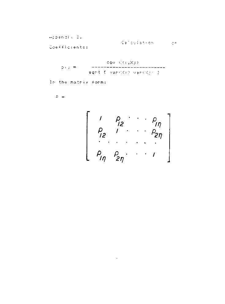
p e n ? i

C o e + t i c i e n t =

coy '':< i ,X.j >

P , _;

=

=qr t [ Mar '":< i ;

In the ma t r i x t orm :

?r

/ ^*

'

P12 in

p 1 -

p/<? H2rj

A P -

i"7 2rj

RUN NAME

INPUT ME

N OF CAS

VARIABLE

INPUT FO

1'ISCRIMI

OPTIONS

Si-AD INP-

i 7 ^ q i

1 j 2 1 8 . 8

t "> ~i O O T;

I <1 64.57

15 36.31

IS 93.33

17 3.510

97.72

63.10

831 .8

214.5

2.240-i --. j

1 "7 OO

1 9 9 5

"! "7 'J p

39 . 02

5.010

DIUM

LIST

RMAT

NA,-;T

THESIS SYNTHETIC DATA RATIO-SET ANALYSIS

CARD

4

CASE . ID , EX1 , EX2 . EX3 , EX4 , EX5/

FREEFIELD

GROUPS = CASE ( 1.4) /VARIABLES = EX1.EX2.

ANALYSIS = CASE /METHOD = WILKS/

1 3 . 5 . 6 . 7 . 3 , 1 1 . 1 2 , 1 7 ,:.?;. 9

UT DATA

-i i

'= 4

4 4

45

46

1-

Cl cr

7~

4 . 2

2 . 0 4 0

5 . 0 1 0

9.950

2.690

1202

61 .66

36.31

134.0

6.310

114.8

72.44

391.3

15.85

9.12

23.4 4

2.750

147.9

14.45

2754

T! OCi

1"

. 2 3

25.70

3.390

45.71

n f. q n

6 60.7

2.510

6. "60

9 - 9 5 0

2.690

195.0

73. S

U1 -'

-L X

70.79

^ 51 *>

154.9

1071

75.8 6

20 8.4

1122

38.90 33.90 40.74

125.9 125.9 144.5

7-940

97.72

41.69 44.67 63.10

1000 1000 977.2

15.49 15.35 13.49

11 .48 13.13 12.30

23.44 21.83 21.83

3.160 2.510 2.240

133.0

14.45

10.00 7.940

109.7 109.2

44.67

1000

15.35

22.91

44.67

2.510-

n oq

14. 4.5

7 4 1 . 3

n o 2 0

. 7'. 2 0

1 4 ,. 1 3

147. q

13.1 2

1698

26.9 f~>

15.8 j

H

13.62

2188

2.92

18.62

21 .62

i- -i n q

20. 41

794.3

2.690 2.3.60

6.310 6.460

19.95 12.5 0

2.240 3.160

3.160

4 5.71

23.84

7 ,rl '? Ci

:mti^ r, t _-r.d Sup;., ; ^

"

i 9"

?Oicut M i erode ns i tome ter . Gratis PFHS S'

- McBeth RD-100 Reflection Densitometer

-

Landsat 2 Mu 1 t i spec tral Scene 21685-17255

- 'Jr i ted Geol ogi cal Survey Maps

Test reck t>pes supplied, Misco Siolooical I r ;

ri^2.-29

; n c 1 u d i n g the -f o 1 1 ow i n q r oc k t >r. * = ;

3uar tz ti

Gr e y S 1 a'

Graph te

4. ~ed SI i. te

i . Wh i te Mart

o 0 a k wratten filters,*2 , ?3 ,

Kodak High Speed In -fared F i 1 m

;t i ti a g e r / J

Kodak Fine Gra i n Fos i t i we F i'

m

rati o i mage J

. r,o a k 'J e r s ama t F i ! mF1

<-

; c e s = o r , !

''-I- 11730 Computer3.''

stem, SFSb

'"4 r.nd

2481 (ESTr

T I' f T,!-;, , ._

-

'. o n t r ? s t C = J c u ! 5 r ! o pcr

J LI ST

2 DIM ARR(2>: DIM ADD<2)

5 GOTO 25

10 REM THIS PROGRAM IS MADE

FOR THE THES

IS RESEARCH

PROJECT OF D.J.MARSH

MADE DURING THE

QUARTER 832

15 REM THE FOLLOWING PROGRAM

WILL SOLVE A

SET OF

ANALYTICAL EQUATIONS FOR

MASK CONTRAST VA

LUES FOR

18 REM THE PROJECT "PHOTOMETRIC

PROCESSING A

ND INTERPRETATION

OF RATIOED IMAGERY FOR

SEPARATION OF GR

OUND FEATURES.

20 REM ********************

25 HOME

30 VTAB 10: HTAB 5

35 INVERSE : FLASH : PRINT "WELC

OME TO THESIS PROGRAM1"

37 VTAB 1 1 : HTAB 10

40 PRINT "BY DONMARSH."

45 NORMAL

50 FOR I = 1 TO 1000

51 NEXT I

80 GOSUB 1000

85 PRINT "PLEASE INPUT THE TWO S

PECTRAL BANDS ": PRINT "BEIN

GUSED."

90 INPUT Al ,A2

95 GOSUB 1000: PRINT "WHICH SPEC

TRAL BAND WILL BE COPIED": PRINT

"EXACTLY WITH THE INVERSE S

IGN CONTRAST""'

97 INPUT RR

100

105

120

125

130

GOSUB 1000: PRINT'

CONTRAST VALUE OF": PRINT

"

BAND"RR

INPUT Zl

GOSUB 1000: PRINT'

INPUT THE

SPECTRrtL

PLEASE

135

190 l

200

300 1

310 A

320 B

330 C

340 D

350 E

360 F

370

372

374

400

410

425

426

430

440

999

1000

1001

IN

PUT MAXIMUM AND MINIMUM": PRINT"

EXPOSURE VALUES FORBAND"

:

PRINT Al

INPUT XI ,X2

GOSUB 1000: PRINT "INPUT MAX

IMUM AND MINIMUMEXPOSURE"

: PRINT"

VALUES FOR BAND"

: PRINT A

2

INPUT YI ,Y2

GOTO 300

REM

REM

= XI / X2

= YI / Y2

= X2 / XI

= (XI - 1) / (X2 - 1)

= (YI - 1) / <Y2 - 1 >

= Y2 / YI

PRINT "*********************

PRINT "*** OUTPUT CONTRAST V

ALUES***"

PRINT "*********************

*********"

FOR E2 = <Zi - 0.5) TO <21 +

0.5) STEP 0.05

El = (0.4342945 * LOG CO) +

(0.4342945 * LOG ( ABS ((D +

E) - (10AE2) * F))>

PRINT "ORTGIONALCOPY"

PRINT" CONTRAST CONTRAS

T"

PRINT E2,E1

NEXT E2

GOTO 1001

HOME : VTAB 13: RETURN

END

Hpp end i x Annotation of Test Sites andNam*"

Number Site Name

Rocks

1 1 & 15

2 2 & 9

3 & 16

4 4 & 5

6 /

7 3

8 10

9 1 1

10 12

1 1 13

12 14

13 17

14 18

15 19

Lake Bonn i v i 1 1 e

Depos i ts

Mi ocenc Vol can i c

0 1 i goc e n e Vo 1 c an i c

Rock

Bal sal t and

Rhyol i te

01 der All uv i al

D e p os i t s

McCoy Creek

& S h e p r oc k Gr cu

Temp 1 e Bu t te

Format i ons

Lands 1 i des

Navajoe Sandstone

Prospect Mountain

Guar tz i te

Wh i te Sage

Format i ons

Al 1 uv i urn and

Col 1 uv i urn

Bal sal ts

Cre taceou =

Format i ons

Arap i an Shal e

VITA

Don is a fourth year student at the Rochester

Institute of Technology seeking a Bachelors degree i r,

Imaging and Photographic Science. Don has li'^ed in the

Rochester area for most of his life and became interested

in photography his 9th grade of high school. Pursuing his

interest in science and photography, Don started his

college career in 1980 at R.I.T. and became amember-

c.f

several photographic interest groups. Continuing an

interest in remote sensing and digital image processing,

Don hopes to complete a Masters degree in this discipline

in the near future.