No.07-E-5 February 2007

Phillips Correlation and Trend Inflation under the Kinked Demand Curve Toyoichiro Shirota*

toyoichirou.shirota@boj.or.jp Bank of Japan 2-1-1 Nihonbashi Hongoku-cho, Chuo-ku, Tokyo 103-8660

* Economic Analysis, Research and Statistics Department Papers in the Bank of Japan Working Paper Series are circulated in order to stimulate discussion and comments. Views expressed are those of authors and do not necessarily reflect those of the Bank. If you have any comment or question on the working paper series, please contact each author. When making a copy or reproduction of the content for commercial purposes, please contact the Public Relations Department (webmaster@info.boj.or.jp) at the Bank in advance to request permission. When making a copy or reproduction, the source, Bank of Japan Working Paper Series, should explicitly be credited.

Bank of Japan Working Paper Series

Phillips Correlation and Trend Inflation

under the Kinked Demand Curve

Toyoichiro Shirota†,‡

February, 2007

Abstract

This paper explains the weak ’Phillips correlation’ under low trend inflation.

This correlation is confirmed empirically but the standard sticky price models fail

to account for it. This paper extends the standard sticky price model to the case of

the ”smoothed off kinked” demand curve, which is typically regarded as a source

of the strategic complementarity. Our results suggest that the kinked demand curve

can offer an appropriate explanation to fill this gap between the theoretical impli-

cation and the empirical facts.

JEL classification: E31, E32

Keywords: sticky prices; trend inflation; kinked demand curve

†Research and Statistics Dept., Bank of Japan; e-mail:toyoichirou.shirota@boj.or.jp‡I thank seminar participants at the Bank of Japan and other members of research staff for comments.

The analysis and conclusions set forth are those of the author and do not indicate concurrence by other

members of the research staff or the Bank of Japan.

1

1 Introduction

It is a conventional view that the output-inflation correlation, the ’Phillips correlation’,

is weak under the low trend inflation environment. Ball, Mankiw, and Romer (1988)

(hereafter BMR) suggest that the short-run Phillips curve depends on the average rate

of inflation, and that it becomesflatter when the average rate of inflation declines. Re-

cently, Benati (2007) statistically verifies the BMR’s argument, using the data from the

post-WWII OECD countries. He concludes that”the Phillips trade-off Alan Greenspan

was facing towards the end of 1980s was not the same as the one faced by Paul Volcker

at the beginning of the decade.”

However, the standard sticky price models, which occupy the predominant posi-

tion in the recent monetary policy analysis,1 fail to account for these empirical facts.

Notably, Ascari (2004) first finds that the slope of the new Keynesian Phillips curve

(NKPC) becomessteeperunder lower trend inflation. Further, Ascari and Ropele

(2007) investigate the general equilibrium outcomes of trend inflation in the standard

sticky price models. Their results suggest that the Phillips correlation comes to be

strongerunder low trend inflation than under high trend inflation. These theoretical

implications of trend inflation are not consistent with the empirical facts.

A limitation of the standard sticky price models is that it assumes the demand faced

by a price-setter has a constant elasticity (CES) form. This assumption implies that

the quantity of demand for a fixed-price product grows explosively under positive trend

inflation. Then, the expected response of the future demand is highly sensitive to the

relative price variations, with the flatter slope of the demand curve. Consequently,

firms come to be more reluctant to charge the cost variations onto the current prices,

thus making the price level responses more sluggish under the positive inflation envi-

ronment.

This paper proposes a new mechanism, which can help to capture the desired re-

1The sticky price model with the Calvo (1983) type infrequent price adjustment and the monopolistic

competition is the workhorse in this literature. It is used to study various topics such as the monetary

policy rules (e.g.,Goodfriend and King (1997); Clarida, Galı, and Gertler (1999); Woodford (2003)),

the optimal monetary policy (e.g.,Aoki (2001); Woodford (2003)) and inflation dynamics (e.g.,Galı and

Gertler (1999); Sbordone (2002)). Most of these research typically assume zero trend inflation at the

steady state and log-linearize around zero inflation.

2

sponses of demand, over the current research on the trend inflation. To be specific, we

replace the CES demand curve in the standard sticky price model with the ’smoothed

off kinked’ demand curve (Kimball (1995)), wherein consumers flee from relatively

expensive products but do not flock to inexpensive ones. The kinked demand is ex-

pected to avoid the extreme expansion of the demand for the relatively cheap goods

and to overcome the discrepancy of the new Keynesian models under trend inflation.

Moreover, recent empirical evidence from scanner data gives a support to incorporate

the kinked demand curve in the general equilibrium settings (Dossche, Heylen, and den

Poel (2006)).

In general, the kinked demand curve is considered to generate the endogenous

persistence through the strategic complementarity among the price-setters (Kimball

(1995), Bergin and Feenstra (2000) and Dotsey and King (2005)).2 This paper aims

to extend these studies to the trend inflation issues. Namely, employing the Kimball

(1995) type kinked demand curve, we derive the NKPC under the a la Calvo sticky

price setting and investigate the effect of trend inflation in a simple general equilibrium

models.3

We are successful in making clear the following two points; (i) contrary to the ex-

isting theoretical results of the typical sticky price models, the coefficient of the NKPC

under the kinked demand is increasing with respect to the rise of the trend inflation rate;

(ii) embedding our NKPC into a simple dynamic general equilibrium model, we show

the greater impulse response of output and the smaller reaction of inflation to a shock

under low trend inflation. It is concluded from our analytical results that the kinked

demand explains the gap between the theoretical implication of the new Keynesian

models and the empirical facts.

Concerning to the flatter slope of the Phillips curve under low inflation, the past

2Kimball (1995) first incorporates the smoothed off kinked demand curve in the sticky price model

as a source of the real rigidity. Although Kimball (1995) employs the concave demand aggregator in

an implicit form, Bergin and Feenstra (2000) adopt the explicit trans-log demand aggregator. Moreover,

Dotsey and King (2005) give the specific function form to the Kimball’s type concave demand aggregator.

All there studies are motivated to generate the endogenous persistence in the sticky price models and do

not mention the role of the non-zero trend inflation rate.3Dotsey and King (2005) introduce Kimball (1995)’s demand into the state-dependent pricing model

of Dotsey, King, and Wolman (1999).

3

literature has stressed the role of the time-varying price rigidities. BMR and Romer

(1990) claim that the frequency of the price adjustment is lower under the low inflation

environment. Recently, Bakhshi, Burriel-Llombart, Khan, and Rudolf (2003) apply

the Romer (1990)’s idea to the typical sticky price model and derive the flatter slope

of the NKPC under low inflation. Besides, Tobin (1972) and Akerlof, Dickens, and

Perry (1996) claims that the unemployment rate increases under the low inflation period

because the nominal prices and the nominal wages tend to be more rigid downwards

than upwards. Consequently, the Phillips curve is flattering when the inflation rate is

near zero.

Our approach complements to these line of research but is different from theirs in

that we intend to shed light on the real rigidities from the demand behavior, instead of

the rigidities in the price-setting behavior or the wage-setting behavior.

The next section presents the model structure, highlighting the use of Kimball

(1995) and Dotsey and King (2005) concave demand aggregator. Section three shows

the generalized NKPC. Section four discuss the role of the kinked demand curve. Sec-

tion five compares the equilibrium dynamics of low trend inflation and that of high

trend inflation under the Kimball’s demand aggregator. Finally, section six concludes

the paper.

2 The model

We construct a simple monopolistic competition sticky price model to clearly illustrate

the implication of trend inflation under the ”smoothed off kinked” demand curve. In

our setup, production is linear in labor input, and consumption and labor effort are

separable in utility. Thus, trend inflation and the kinked demand are the key features

in this model. To begin with, we specify the Kimball (1995) type demand aggregator,

following Dotsey and King (2005). Then, the settings of the economy is present.

2.1 Kimball demand aggregator

We assume that any price-setter indexed byi ∈ (0,1) is a monopolistic competitor

who produces a differentiated goodi. Letting D(·) the demand aggregator, the cost

4

minimization problem of a representative household is,

min{Ct(i)}

∫ 1

0Pt(i)Ct(i)di s.t.

∫ 1

0D

(Ct(i)Ct

)di = 1.

whereCt(i), Ct, andPt(i) is the consumption of a goodi, the aggregated consumption

and the nominal price of a goodi, respectively. Ct is implicitly defined, given the

demand aggregatorD(·). Kimball (1995) presumes a functionD(·) sufficesD(1) =

1,D(·)′ > 0, andD(·)′′ < 0, for all Ct(i)/Ct > 0.

Here, we specify the function form of the aggregator, as in Dotsey and King (2005).

D(Ct(i)) =1

(1 + η)γ

[(1 + η)Ct(i) − η

]γ −[1 +

1(1 + η)γ

](1)

whereCt(i) ≡ Ct(i)/Ct, γ ≡ (ε(1 + η) − 1)/(ε(1 + η)), andε > 1.

In this function form, we have one more parameter,η, compared to the Dixit and

Stiglitz (1977) type CES function form. This parameter determines the curvature of the

demand curve. Furthermore, in the case ofη = 0, D(·) reduces to the CES demand

aggregator.

Solving the cost minimization problem gives the following inverse demand func-

tion,

Ct(i)Ct

=1

1 + η

(Pt(i)

Pt

λt

) 1γ−1

+ η

(2)

wherePt(i) ≡ Pt(i)/Pt andλt is the Lagrange multiplier. Denotingd(·) as the inverse

function ofD(·)′, λt/Pt suffices∫ ∞

0D(d(Pt(i)/λt))di = 1. Explicitly, λt/Pt is expressed

as,

λt

Pt=

∫ 1

0

(Pt(i)Pt

)γ/(γ−1)

di

γ−1γ

. (3)

An advantage of employing this sort of the demand specification is that it enables

to derive the aggregate price index as follows.

Pt =1

1 + η

[∫ 1

0Pt(i)

γγ−1 di

] γ−1γ

+η

1 + η

∫ 1

0Pt(i)di. (4)

Eq.(4) means that the aggregate price index is expressed as a sum of the CES type

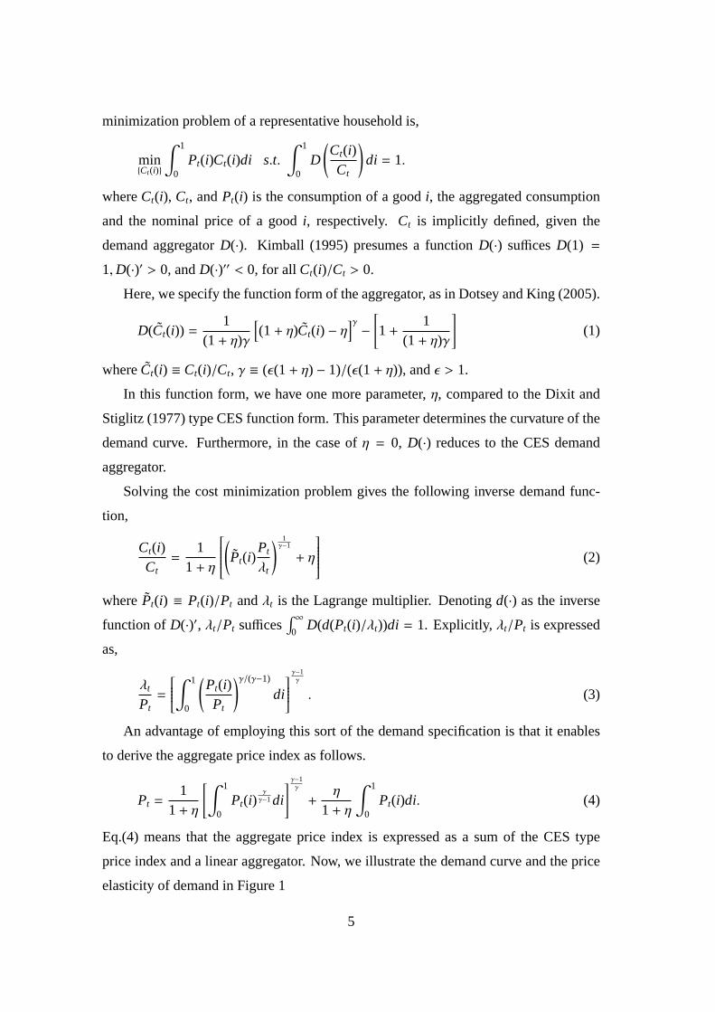
price index and a linear aggregator. Now, we illustrate the demand curve and the price

elasticity of demand in Figure 1

5

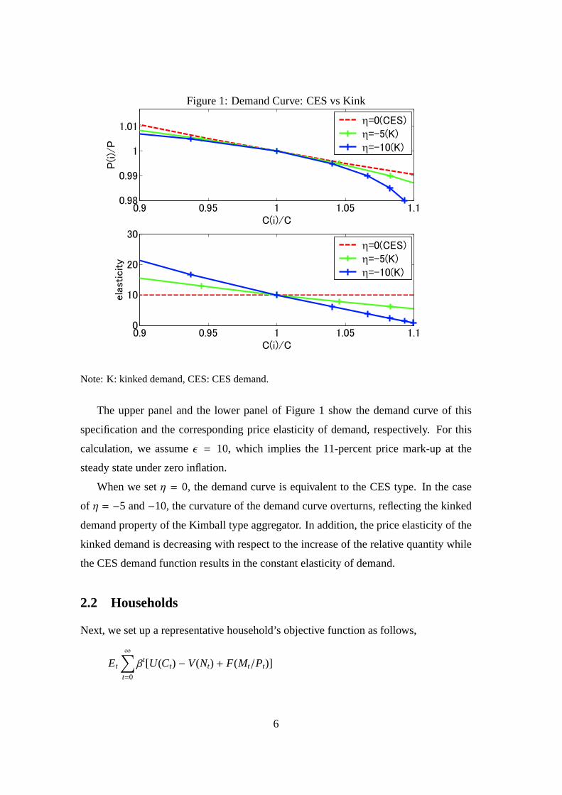
Figure 1: Demand Curve: CES vs Kink

Note: K: kinked demand, CES: CES demand.

The upper panel and the lower panel of Figure 1 show the demand curve of this

specification and the corresponding price elasticity of demand, respectively. For this

calculation, we assumeε = 10, which implies the 11-percent price mark-up at the

steady state under zero inflation.

When we setη = 0, the demand curve is equivalent to the CES type. In the case

of η = −5 and−10, the curvature of the demand curve overturns, reflecting the kinked

demand property of the Kimball type aggregator. In addition, the price elasticity of the

kinked demand is decreasing with respect to the increase of the relative quantity while

the CES demand function results in the constant elasticity of demand.

2.2 Households

Next, we set up a representative household’s objective function as follows,

Et

∞∑

t=0

βt[U(Ct) − V(Nt) + F(Mt/Pt)]

6

whereEt, β, Nt, andMt are the conditional expectation operator, the subjective discount

factor, labor hours and the cash holdings, respectively.

The contemporaneous budget constraint for the representative household is,

PtCt + EtDt,t+1Bt+1 ≤WtNt + Πt + Bt + Tt − Mt+1 + Mt (5)

whereEtDt,t+1, Bt, Wt, Πt, andTt are a price of one period contingent claim bond, the

amount of the bond, the nominal wage rate, the dividend from firms and the lump-sum

transfer from the government.

Maximizing the expected life-time utility subject to the demand function of eq.(2)

and the budget constraint of eq.(5), we yield the first order conditions of the following.

Wt

Pt=

Vnt

Uct,

Uct = βEt

[Uct+1Rt

Pt

Pt+1

],

FMt/Pt = −βEtUct+1 + Uct

whereRt = EtDt,t+1−1, andDt,τ = βτ−t(Ucτ/Uct)(Pt/Pτ) are the nominal yield of the

bonds and the stochastic discount factor. A subscript onU, V, andF denotes the partial

derivative of the function.

Hereafter, we parameterize utility functions asU(C) = ln(C),V(N) = N, and

F(M/P) = am(M/P)1−γm/(1− γm), for analytical simplicity.

2.3 Firms

Let the production function of a firmi as follows.

Ct(i) = Nt(i).

Solving the cost minimization problem yields the real unit cost asVt/Pt ≡ vt = Wt/Pt.

Firms set their prices in the Calvo fashion such that when a firm gets an opportunity

to reset the price at timet, the firm can choose the optimal price to maximize the

discounted sum of the future profit. The price-reset probability is denoted as 1− α(0 < α < 1). Then, a firm’s optimization problem can be expressed as follows.

maxPt(i)

Et

∞∑

τ=t

ατ−tDt,τ [Pt(i)(1 + τc) − Vτ] Cτ(i) s.t. eq.(2) and eq.(3) (6)

7

whereτc is the sales tax rate.

Solving the profit maximization problem gives the following optimal relative price

equation,

P∗tPt≡ Pt =

1γ(1 + τc)

Et∑∞τ=t (αβ)τ−t Pt

Pτ

(Qτ

Pτ

)1/(γ−1)Vτ

Et∑∞τ=t (αβ)τ−t Pt

Pτ

[(Qτ

Pτ

)1/(γ−1)+ ηγ−1

γ(Pt)−1/(γ−1)

] (7)

whereπt is the inflation rate,Pτ = P∗t (i)/Pτ, andQτ = (λτ/Pτ)−1.

3 The generalized NKPC

3.1 The generalized NKPC under the kinked demand

Log-linearizing eq.(7) around the steady state, we obtain the following generalized

NKPC.

πt = λvt + κEtπt+1 − ω1(1− π)φt+1 − ω2(1− π1/(γ−1))ψt+1, (8)

whereφt =

(1− αβπ−1/(γ−1)

) (YYγ−1πt + vt

)+ αβπ−1/(γ−1)

(φt+1 − 1

γ−1πt+1

)

ψt = αβπ−1(ψt+1 − πt+1

) (9)

and x denotes the log-deviation from its steady state value, ¯x. The detail of the

derivation and each coefficient (κ, λ, ω1, ω2,YY) in eq.(8) are described in Appendix 1.

We can confirm that eq.(8) is equivalent to the standard NKPC under trend inflation

(Ascari (2004)) when we setη = 0. In addition, if the steady state inflation is also zero

(π = 1), it reduces to the standard NKPC (Roberts (1995); Clarida, Galı, and Gertler

(1999)).

3.2 Parameter settings

In order to examine our NKPC and its coefficients, we specify the model parameters.

Table 1 shows the benchmark parameters.

1− α, ε, η, andβ denote the price-reset probability, the price elasticity of demand,

the curvature of the demand curve, and the discount factor. First, we set 1− α = 0.4,

8

Table 1: Parameters

1− α ε η β

0.4 10 -10.0 0.99

assuming that a firm resets the price 1.6 times a year on average. Since Bank of Japan

(2000), who surveys firm’s price setting behavior, reports that the average number of

times to reset prices is one or two times in a year, our parameter setting is consistent

with this evidence. Second,ε corresponds to the price elasticity at the zero inflation.

ε = 10 implies the 11 percent price markup under zero inflation. Third, we specify

η = −10. This value is the medium of Kimball (1995) and Bergin and Feenstra (2000).

Chari, Kehoe, and McGrattan (2000) criticize the curvature of the Kimball (1995)’s

demand is extraordinary. Namely, Kimball (1995)’s parameterization corresponds to

η = −42 in the present Dotsey and King (2005)’s specification. Relative to Kimball

(1995), our parameterization is moderate. Finally, we setβ = 0.99.

3.3 The coefficient of the generalized NKPC and trend inflation

We can point out the two features of our NKPC in eq.(8); (i) each coefficient is the

function of trend inflation in addition to the deep parameters; (ii) as is suggested in

Ascari (2004) and Ascari and Ropele (2007), the additional terms (φt) appear at the

end of the right hand side of eq.(8). Further, we also have another additional term (ψt),

reflecting the introduction of the kinked demand curve. It disappears when the demand

curve is CES type (η = 0). Since these additional terms in eq.(9) include the future

variables, the inflation dynamics becomes more front-loading.

The top panel of Figure 2 illustrates the coefficient of the unit cost, in other words,

the slope of the NKPC. Under the kinked demand, the slope becomes flatter as the

rate of trend inflation declines. Instead, under the CES demand, it becomes steeper as

the rate of trend inflation declines, just like Ascari (2004), Bakhshi, Burriel-Llombart,

Khan, and Rudolf (2003) and Ascari and Ropele (2007). Therefore, the kinked demand

is consistent with the empirical facts of BMR and Benati (2007) at least in the structural

function form; the Phillips curve is flatter under the low inflation environment. In the

9

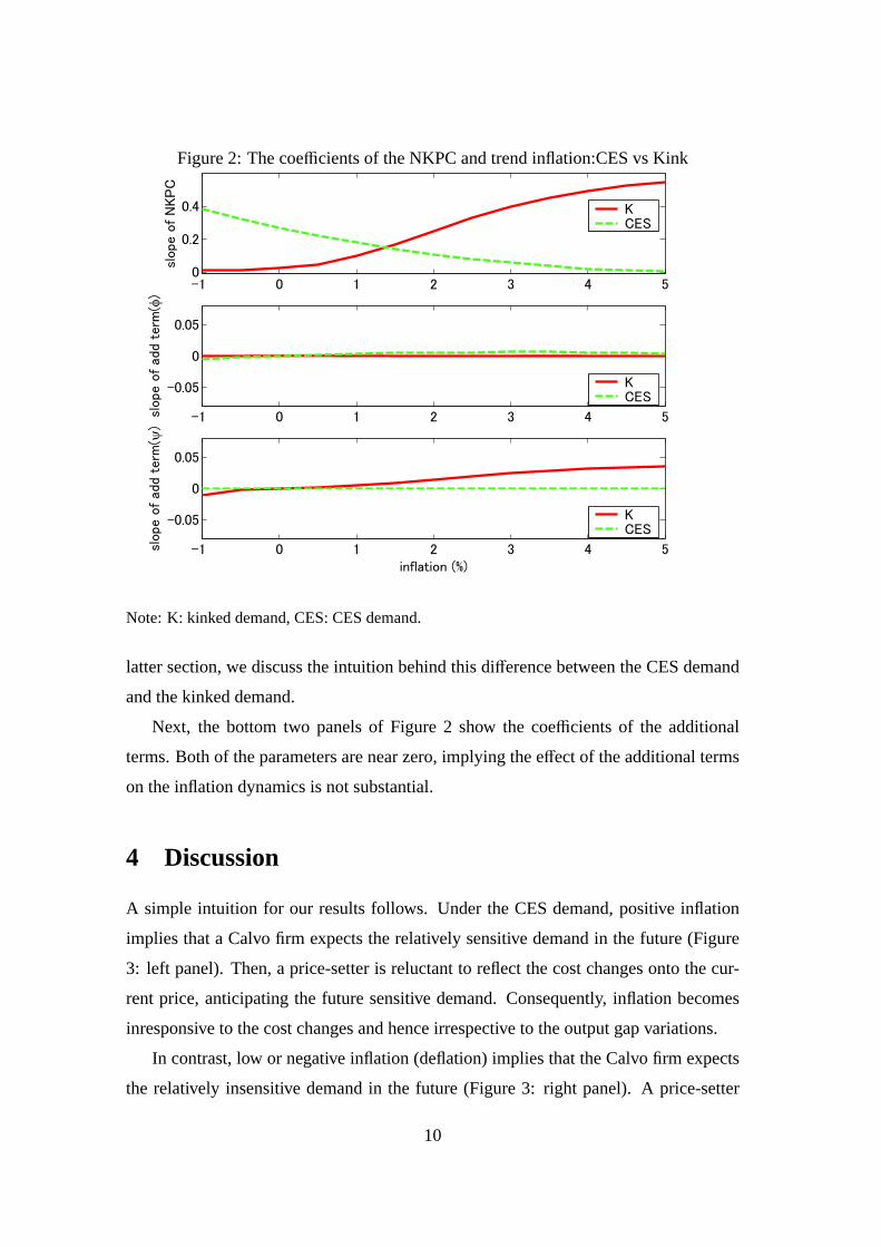
Figure 2: The coefficients of the NKPC and trend inflation:CES vs Kink

Note: K: kinked demand, CES: CES demand.

latter section, we discuss the intuition behind this difference between the CES demand

and the kinked demand.

Next, the bottom two panels of Figure 2 show the coefficients of the additional

terms. Both of the parameters are near zero, implying the effect of the additional terms

on the inflation dynamics is not substantial.

4 Discussion

A simple intuition for our results follows. Under the CES demand, positive inflation

implies that a Calvo firm expects the relatively sensitive demand in the future (Figure

3: left panel). Then, a price-setter is reluctant to reflect the cost changes onto the cur-

rent price, anticipating the future sensitive demand. Consequently, inflation becomes

inresponsive to the cost changes and hence irrespective to the output gap variations.

In contrast, low or negative inflation (deflation) implies that the Calvo firm expects

the relatively insensitive demand in the future (Figure 3: right panel). A price-setter

10

inclines to pass-through the cost changes on the price. Hence, inflation comes to be

more responsible to the variations in output gap and the slope of the Phillips curve

becomes steeper.

Figure 3: Inflation and Demand curve: CES

Figure 4: Inflation and Demand curve: Kink

However, the above mechanism turns around under the kinked demand where con-

sumers flee from relatively expensive products but do not flock to inexpensive ones.

Positive inflation leads to the insensitive demand and negative inflation results in the

responsive demand on average under the kinked demand (Figure 4).

Accordingly, a price-setter is willing to charge the cost changes on the price under

positive inflation and is unwilling to do so under negative inflation. Thus, inflation

responds more to the cost variations under positive inflation and less under negative

inflation. Finally, the slope of the Phillips curve is flatter under low inflation than under

11

high inflation.4

5 Equilibrium dynamics

The analysis in the previous section reveals that the replacement of the CES demand

with the kinked demand successfully helps to overcome the problem of the standard

sticky price model such that the coefficient of the NKPC decreases associated with

the rise of the trend inflation rate. However, the empirical facts are the reduced-form

general equilibrium outcomes. Therefore, we embed our NKPC in a simple general

equilibrium model and examine the Phillips correlation under low and high trend infla-

tion. In order to close the general equilibrium, we employ the money growth rate rule

as the monetary policy rule.

5.1 The money growth rate rules

The log-linearized money growth rate rule is specified as∆mt+1 = ρ∆mt + εt where∆m

andεt denote the money growth rate and the monetary disturbance, respectively. In the

shock simulation, we setρ = 0.8.

5.1.1 System of equations

We can obtain the log-linearized system of the general equilibrium as follows.

yt = yt+1 − r t + πt+1 c− Euler

πt = κπt+1 + λyt − ω1(1− π)φt+1 + ω2(1− π1/(γ−1))ψt+1 NKPC

φt = ξ1πt + ξ2yt + ξ3πt+1 + ξ4φt+1 additional term1

ψt = ζ1πt+1 + ζ2ψt+1 additional term2

∆mt+1 = ρ∆mt + εt development o f money

r t = yt − γm(mt − pt) interest rate

whereyt, r andπ are output gap, interest rate, and inflation rate.

4In Appendix 2, we demonstrate that the slope of the NKPC depends on the curvature of the demand

curve and becomes steeper as the curvature of the demand curve increases.

12

5.1.2 Simulation results

Figure 5: money growth rate rules: monetary policy shock

In Figure 5, the upper panel and the lower panel correspond to the impulse re-

sponses of output gap and inflation to a one percent positive money growth rate shock,

respectively. In each panel, the dotted line represents the case of the high inflation (61/4

percent/ quarter) economy and the solid line is the case of the low inflation (0 percent)

economy.

In the figure, we can see the clear difference between the high trend inflation en-

vironment and the low trend inflation environment. In the high (non-zero) inflation

economy, the impulse response of output gap is positive and large. The inflation also

responds in large amount to the shock. The simulation result clearly exhibits the tight

13

linkage between output gap and inflation in the high inflation period.

In contrast, in the low (zero) inflation economy, the impulse response of output gap

is greater and more persistent. The inflation rate responds weakly but persistently to the

shock. The linkage between the real economic activities and the inflation rate becomes

weaker in the low inflation economy.

In addition, the simulation results add a new insight into the literature on the persis-

tent response of output, which is initiated by the Chari, Kehoe, and McGrattan (2000)’s

critique of sticky price models. Similar to Bergin and Feenstra (2000) and Dotsey and

King (2005), we demonstrate that the concave demand aggregator generates the en-

dogenous persistence in the low inflation environment. However, we also shows that

the endogenous persistence disappears in the high inflation environment. Thus, the

inner propagation mechanism depends on the level of the trend inflation rate and it

disappears as the trend inflation rises.

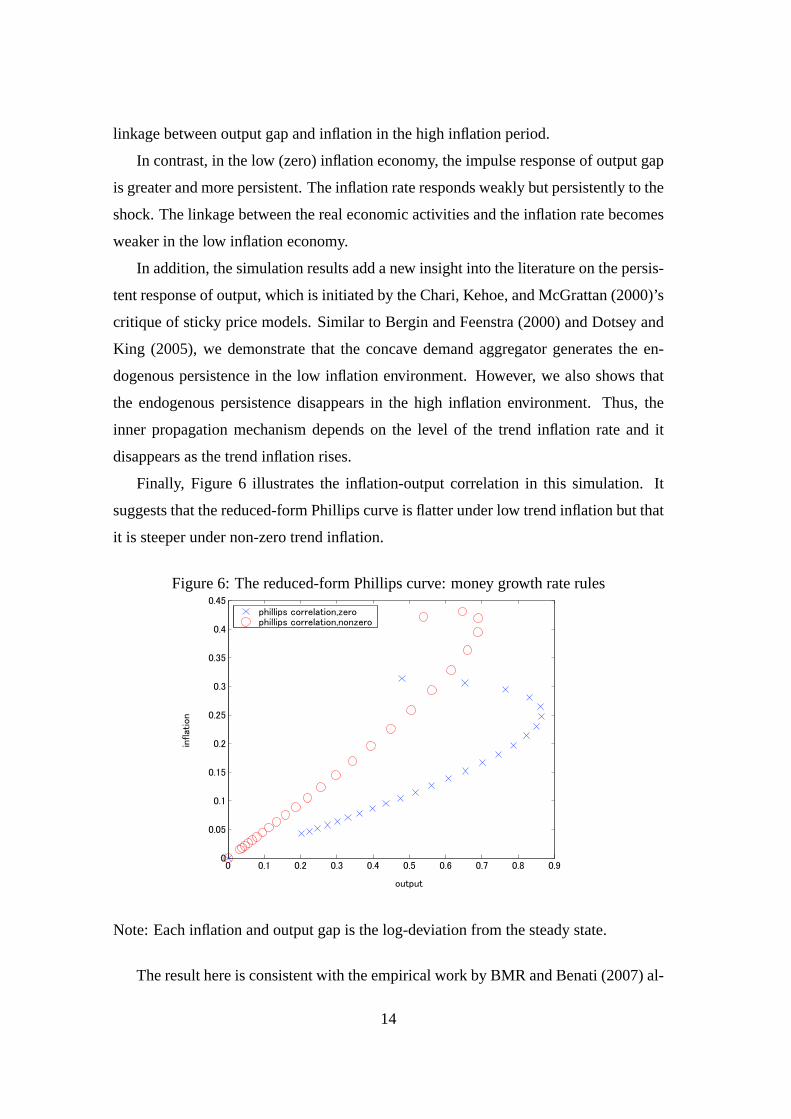
Finally, Figure 6 illustrates the inflation-output correlation in this simulation. It

suggests that the reduced-form Phillips curve is flatter under low trend inflation but that

it is steeper under non-zero trend inflation.

Figure 6: The reduced-form Phillips curve: money growth rate rules

Note: Each inflation and output gap is the log-deviation from the steady state.

The result here is consistent with the empirical work by BMR and Benati (2007) al-

14

though Ascari (2004), Bakhshi, Burriel-Llombart, Khan, and Rudolf (2003) and Ascari

and Ropele (2007) suggest that the canonical sticky price model cannot explain this

empirical fact. Our analysis is successful in explaining this discrepancy between the

standard sticky price models and the empirical evidence. Notably, the mechanism be-

hind our results is different with Bakhshi, Burriel-Llombart, Khan, and Rudolf (2003),

which stress the role of time-varying nominal rigidities in the spirit of BMR or Romer

(1990). We have shown that the kinked demand can also explain the weak Phillips

correlation under low trend inflation.

6 Conclusion

This paper challenges to fill the gap between the implication of the standard sticky price

models and the empirical fact about the ’Phillips correlation.’ We show that introducing

the ’smoothed out kinked’ demand curve (Kimball (1995)) helps to explain the flattered

Phillips curve under the low trend inflation environment.

It would be useful to extend our work to the other situations of pricing, such as the

incomplete exchange rate pass-through. As is suggested in Taylor (2000), the rate of

the exchange rate pass-through is decreasing along with the decline of the inflation rate.

The mechanism developed here might be helpful in explaining this phenomenon.

In order to shed light on the role of the real rigidity from the demand side and

to keep consistency with the existing research by Ascari (2004), Bakhshi, Burriel-

Llombart, Khan, and Rudolf (2003) and Ascari and Ropele (2007), we employ the

time-dependent Calvo type sticky price models. We do not mean to claim that the

Calvo model is innocuous. It is the hotly-debated issue whether the price adjustment

mechanism is approximated by the time-dependent rule or the state-dependent rule.

Yet, our analytical results suggest that the demand structure is also crucial to study the

effect of the trend inflation in the staggered price adjustment models.

In this paper, we do not mention the reason why trend inflation is not zero. However,

recent inflation targeting countries adopt the non-zero positive target rate. In addition,

the actual data suggests that the long-run inflation rate is not zero around the world.

Since the results of the standard model are sensitive to the special assumption of zero

inflation at the steady state, it is worthwhile to keep studying the trend inflation issues.

15

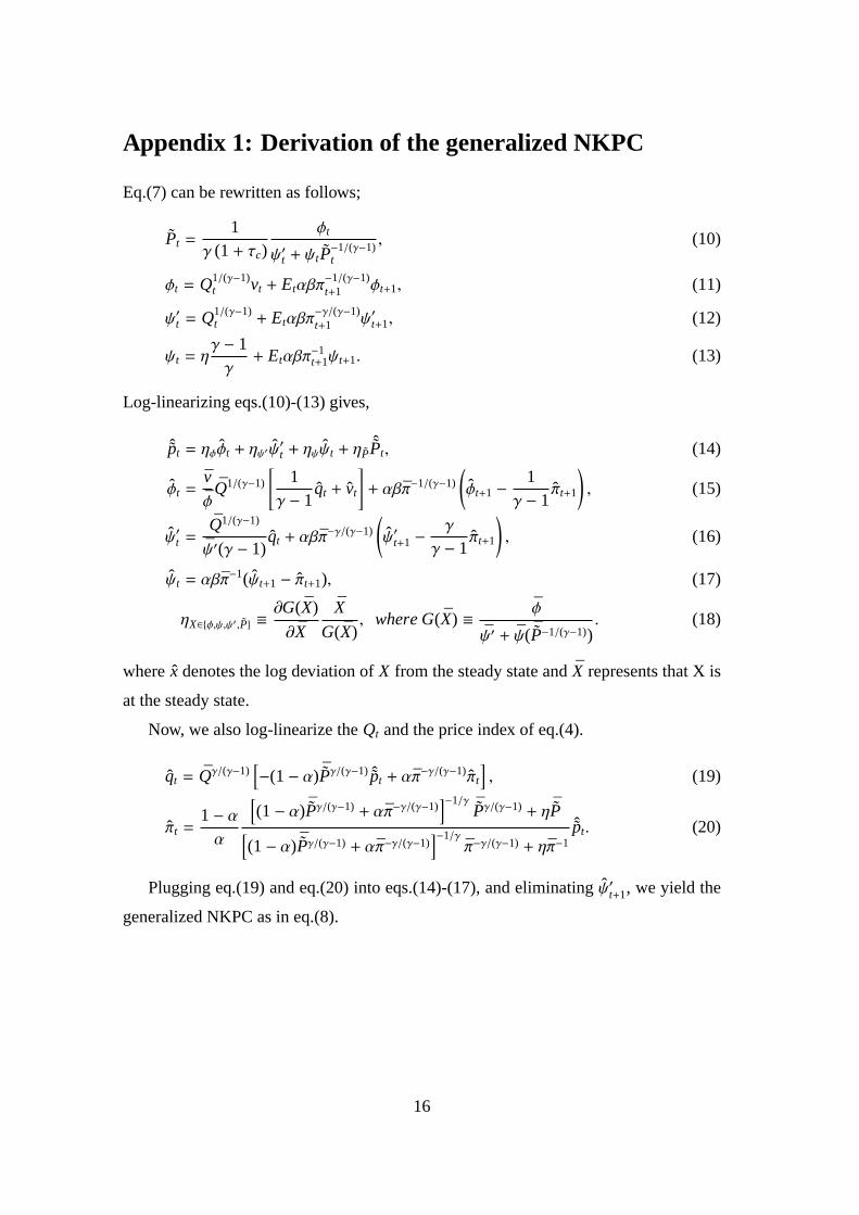
Appendix 1: Derivation of the generalized NKPC

Eq.(7) can be rewritten as follows;

Pt =1

γ (1 + τc)φt

ψ′t + ψtP−1/(γ−1)t

, (10)

φt = Q1/(γ−1)t vt + Etαβπ

−1/(γ−1)t+1 φt+1, (11)

ψ′t = Q1/(γ−1)t + Etαβπ

−γ/(γ−1)t+1 ψ′t+1, (12)

ψt = ηγ − 1γ

+ Etαβπ−1t+1ψt+1. (13)

Log-linearizing eqs.(10)-(13) gives,

ˆpt = ηφφt + ηψ′ψ′t + ηψψt + ηP

ˆPt, (14)

φt =v

φQ1/(γ−1)

[1

γ − 1qt + vt

]+ αβπ−1/(γ−1)

(φt+1 − 1

γ − 1πt+1

), (15)

ψ′t =Q1/(γ−1)

ψ′(γ − 1)qt + αβπ−γ/(γ−1)

(ψ′t+1 −

γ

γ − 1πt+1

), (16)

ψt = αβπ−1(ψt+1 − πt+1), (17)

ηX∈{φ,ψ,ψ′,P} ≡∂G(X)

∂X

X

G(X), where G(X) ≡ φ

ψ′ + ψ( ¯P−1/(γ−1)). (18)

wherex denotes the log deviation ofX from the steady state andX represents that X is

at the steady state.

Now, we also log-linearize theQt and the price index of eq.(4).

qt = Qγ/(γ−1)[−(1− α) ¯Pγ/(γ−1) ˆpt + απ−γ/(γ−1)πt

], (19)

πt =1− αα

[(1− α) ¯Pγ/(γ−1) + απ−γ/(γ−1)

]−1/γ ¯Pγ/(γ−1) + η ¯P[(1− α) ¯Pγ/(γ−1) + απ−γ/(γ−1)

]−1/γπ−γ/(γ−1) + ηπ−1

ˆpt. (20)

Plugging eq.(19) and eq.(20) into eqs.(14)-(17), and eliminatingψ′t+1, we yield the

generalized NKPC as in eq.(8).

16

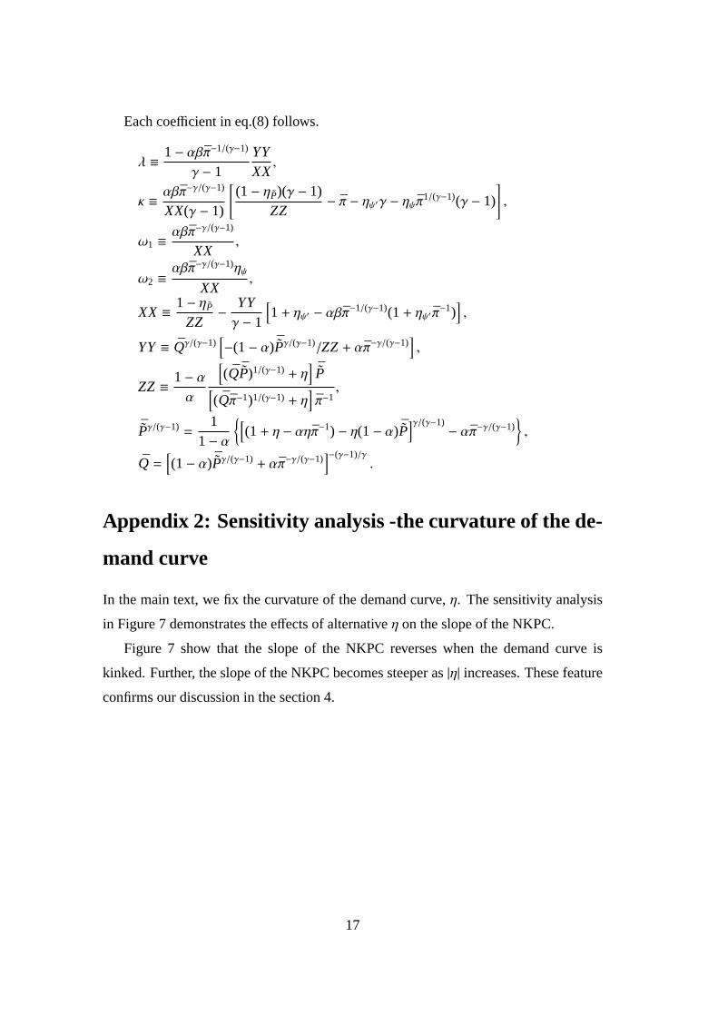
Each coefficient in eq.(8) follows.

λ ≡ 1− αβπ−1/(γ−1)

γ − 1YYXX

,

κ ≡ αβπ−γ/(γ−1)

XX(γ − 1)

[(1− ηP)(γ − 1)

ZZ− π − ηψ′γ − ηψπ1/(γ−1)(γ − 1)

],

ω1 ≡ αβπ−γ/(γ−1)

XX,

ω2 ≡αβπ−γ/(γ−1)ηψ

XX,

XX ≡ 1− ηP

ZZ− YYγ − 1

[1 + ηψ′ − αβπ−1/(γ−1)(1 + ηψ′ π

−1)],

YY≡ Qγ/(γ−1)[−(1− α) ¯Pγ/(γ−1)/ZZ + απ−γ/(γ−1)

],

ZZ ≡ 1− αα

[(Q ¯P)1/(γ−1) + η

] ¯P[(Qπ−1)1/(γ−1) + η

]π−1

,

¯Pγ/(γ−1) =1

1− α{[

(1 + η − αηπ−1) − η(1− α) ¯P]γ/(γ−1) − απ−γ/(γ−1)

},

Q =[(1− α) ¯Pγ/(γ−1) + απ−γ/(γ−1)

]−(γ−1)/γ.

Appendix 2: Sensitivity analysis -the curvature of the de-

mand curve

In the main text, we fix the curvature of the demand curve,η. The sensitivity analysis

in Figure 7 demonstrates the effects of alternativeη on the slope of the NKPC.

Figure 7 show that the slope of the NKPC reverses when the demand curve is

kinked. Further, the slope of the NKPC becomes steeper as|η| increases. These feature

confirms our discussion in the section 4.

17

Figure 7: Sensitivity analysis: -the curvature of the demand curve

η

η

η

η

Note: All parameters except forη are same as in the main text.

Reference

A, G., W. T. D, G. L. P (1996): “The Macroeconomics of Low

Inflation,” American Economic Review, 2, 1–76.

A, K. (2001): “Optimal Monetary Policy Responses to Relative Price Changes,”

Journal of Monetary Economics, 48, 55–80.

A, G. (2004): “Staggered Prices and Trend Inflation: Some Nuisances,”Review of

Economic Dynamics, 7, 642–667.

A, G., T. R (2007): “Optimal Monetary Policy Under Low Trend Infla-

tion,” Journal of Monetary Economics, forthcoming.

B, H., P. B-L, H. K, B. R (2003): “Endogenous Price

Stickiness, Trend Inflation, and the New Keynesian Phillips Curve,” Working paper

Series 191, Bank of England.

18

B, L., G. M, D. R (1988): “The New Keynesian Economics and the

Output-Inflation Trade-Off,” Brookings Papers on Economic Activity, 1, 1–65.

B J (2000): “Price-Setting Behavior of Japanese Companies -The Results of

’Survey of Price-Setting Behavior of Japanese Companies’ and Its Analysis-,”BOJ

Monthly Report.

B, L. (2007): “The Time-Varying Phillips Correlation,”Journal of Mone, Credit,

and Banking, forthcoming.

B, P. R., R. C. F (2000): “Staggered Price Setting, Translog Prefer-

ences, and Endogenous Persistence,”Journal of Monetary Economics, 45, 657–680.

C, G. A. (1983): “Staggered Prices in a Utility-Maximizing Framework,”Journal

of Monetary Economics, 12, 383–398.

C, V., P. K, E. MG (2000): “Sticky Price Model of the Business

Cycle: Can the Contract Multiplier Solve the Persistence Problem?,”Econometrica,

68, 1151–1179.

C, R., J. Gı, M. G (1999): “The Science of Monetary Policy: A New

Keynesian Perspective,”Journal of Economic Litelature, 37, 1661–1707.

D, A., J. S (1977): “Monopolistic Competition and Optimum Product

Diversity,” American Economic Review, 67, 297–308.

D, M., F. H, D. V. P (2006): “The Kinked Demand Curve and

Price Rigidity: Evidence from Scanner Data,” Working Paper 99, National Bank of

Belgium.

D, M., R. J. K (2005): “Implications of State-Dependent Pricing for Dy-

namic Macroeconomic Models,”Journal of Monetary Economics, 52, 213–242.

D, M., R. J. K, A. W (1999): “State-Dependent Pricing and the

Dynamics of Money and Output,”Quarterly Journal of Economics, 114, 655–690.

Gı, J., M. G (1999): “Inflation Dynamics: A Structural Econometric Anal-

ysis,” Journal of Monetary Economics, 44(2), 195–222.

19

G, M., R. K (1997): “An Optimization-Based Econometric Framefork

for the Evaluation of Monetary Policy,” inNBER Macroeconomics Annual 1997, pp.

297–346.

K, M. (1995): “The Quantitative Analytics of the Basic Neomonetarist Model,”

Journal of Money. Credit and Banking, 27, 1241–1277.

R, J. (1995): “New-Keynesian Economics and the Phillips Curve,”Journal of

Money, Credit and Banking, 27, 975–984.

R, D. (1990): “Staggered Price Setting with Endogenous Frequency of Adjust-

ment,”Economics Letters, 32, 205–210.

S, A. M. (2002): “Prices and Unit Labor Costs: A New Test of Price Sticki-

ness,”Journal of Monetary Economics, 49(2), 265–292.

T, J. B.(2000): “Low Inflation, Pass-Through, and the Pricing Power of Firms,”

European Economic Review, 44, 1389–1408.

T, J. (1972): “Inflation and Unemployment,”American Economic Review, 62, 1–

18.

W, M. (2003): Interest Rate and Prices. Princeton University Press.

20