philip mote ÒleadÓ author, chapter 4 nw risa pi, … · adapted from wild et al. (2013). ipcc...
TRANSCRIPT
© Yann Arthus-Bertrand / Altitude
Philip Mote“Lead” Author, Chapter 4
NW RISA PI, Oregon State University
Outline
• 1 slide of climate science
• Background, scope, and processes of IPCC
• Summary of main results
• Observed changes in extremes
• the global warming ‘hiatus’
• Changes in ENSO etc.
Final Draft (7 June 2013) Chapter 2 IPCC WGI Fifth Assessment Report
Do Not Cite, Quote or Distribute 2-127 Total pages: 163
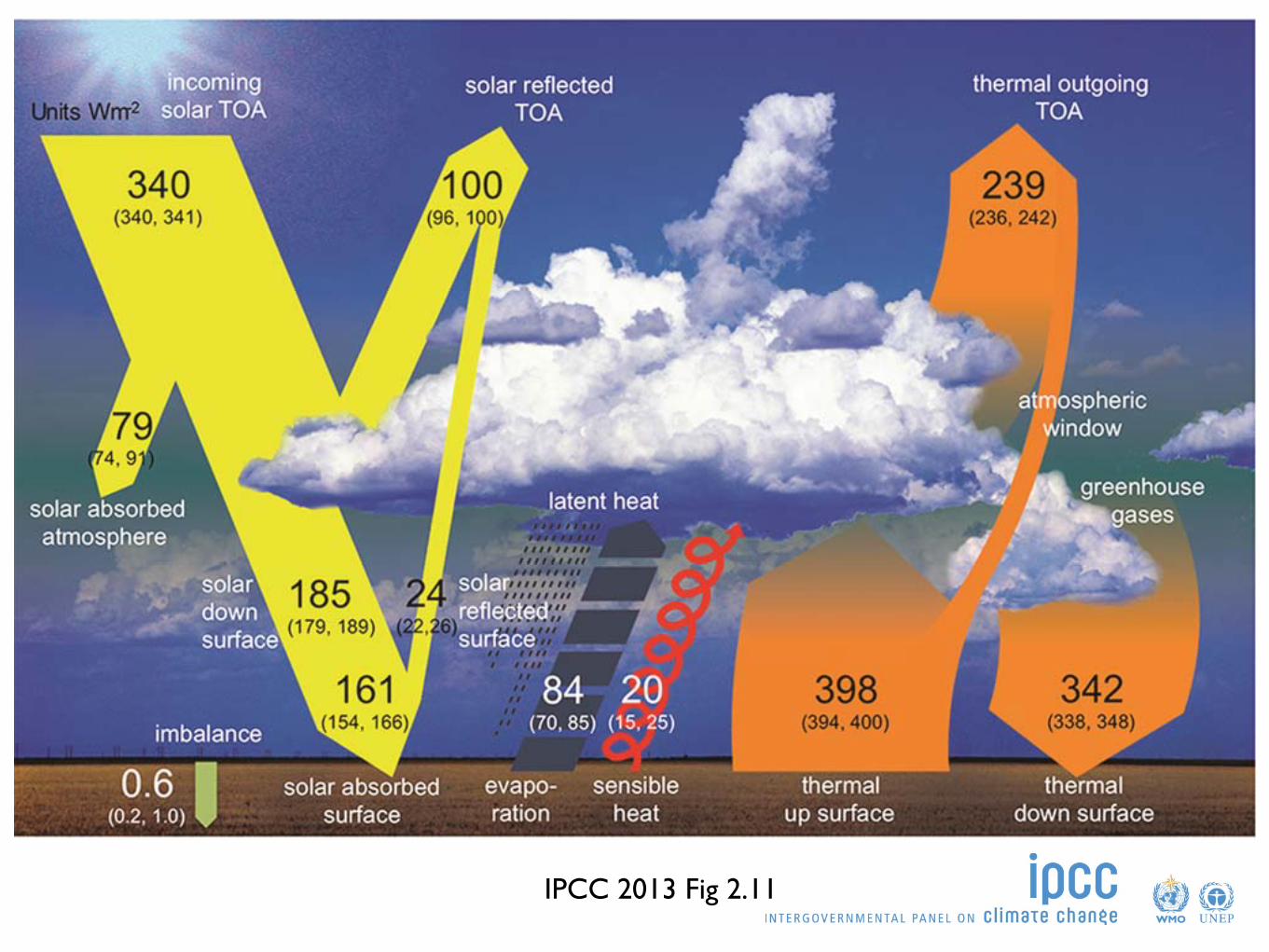
Figure 2.11: Global mean energy budget under present day climate conditions. Numbers state magnitudes of the individual energy fluxes in W/m2, adjusted within their uncertainty ranges to close the energy budgets. Numbers in parentheses attached to the energy fluxes cover the range of values in line with observational constraints. Figure adapted from Wild et al. (2013).
IPCC 2013 Fig 2.11
TSU=technical support unit
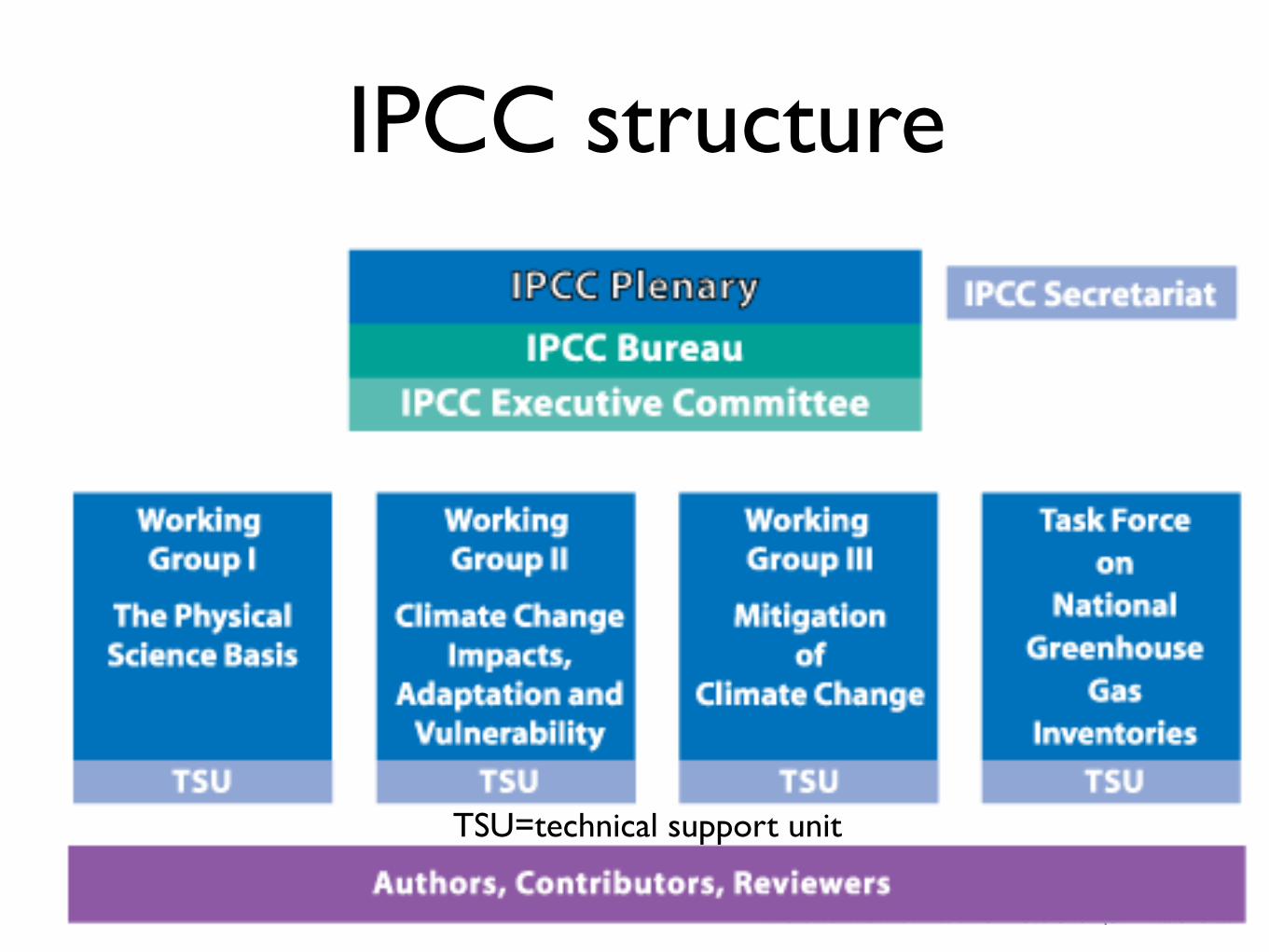
IPCC structure
History
• Established in 1988 WMO-UNEP
• Major assessment reports 1990, 1996, 2001, 2007, 2013
• Numerous special reports
More
• Confidence (very low-low-medium-high-very high)
• Likelihood (quantitative): virtually certain ≥99%, very likely >90%, likely>66%, about as likely as not 33-66%, unlikely <33%, very unlikely <10%, exceptionally unlikely ≤1%.
• Definition of assessment
• Review process: total 54,677 comments
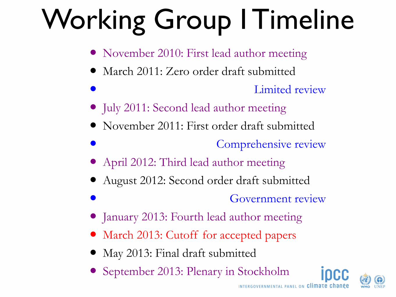
Working Group I Timeline• November 2010: First lead author meeting
• March 2011: Zero order draft submitted
• Limited review
• July 2011: Second lead author meeting
• November 2011: First order draft submitted
• Comprehensive review
• April 2012: Third lead author meeting
• August 2012: Second order draft submitted
• Government review
• January 2013: Fourth lead author meeting
• March 2013: Cutoff for accepted papers
• May 2013: Final draft submitted
• September 2013: Plenary in Stockholm
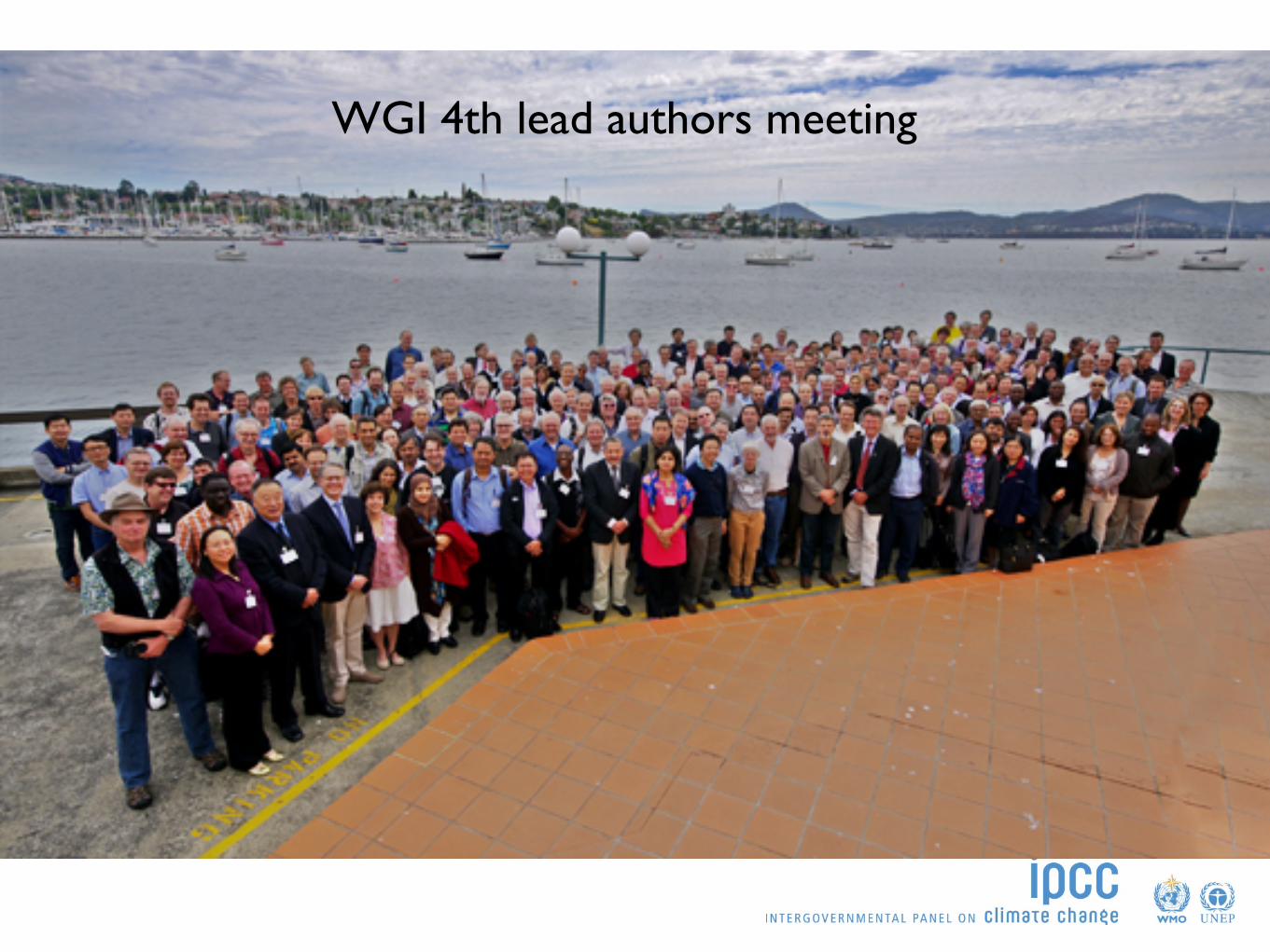
WGI 4th lead authors meeting
Headline statementsWarming of the climate system is unequivocal, and since the 1950s, many of the observed changes are unprecedented ... The atmosphere and ocean have warmed, the amounts of snow and ice have diminished, sea level has risen...
Twelfth Session of Working Group I Approved Summary for Policymakers
IPCC WGI AR5 SPM-27 27 September 2013
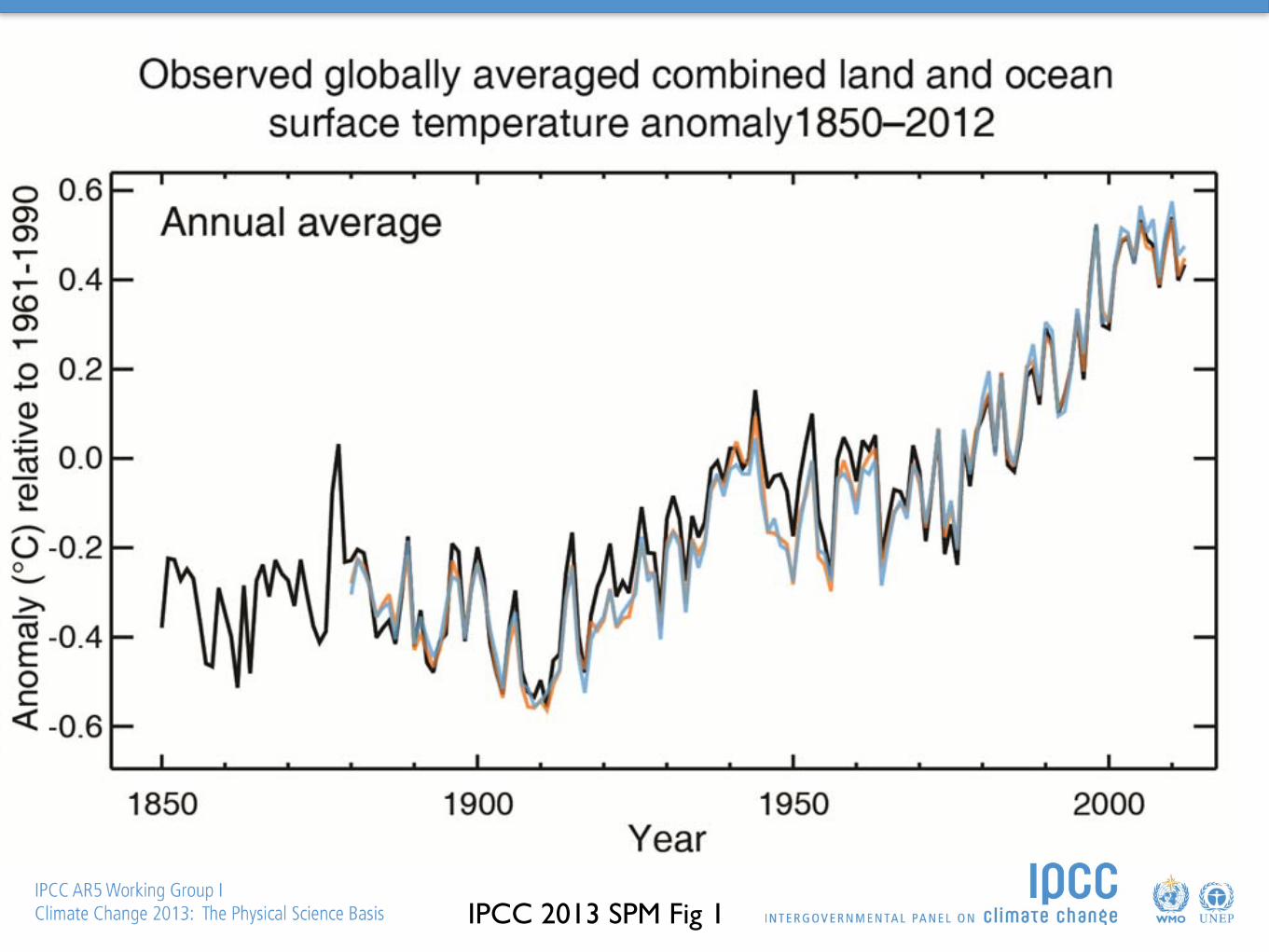
Figure SPM.1 [FIGURE SUBJECT TO FINAL COPYEDIT]
Twelfth Session of Working Group I Approved Summary for Policymakers
IPCC WGI AR5 SPM-27 27 September 2013
Figure SPM.1 [FIGURE SUBJECT TO FINAL COPYEDIT]
Twelfth Session of Working Group I Approved Summary for Policymakers
IPCC WGI AR5 SPM-27 27 September 2013
Figure SPM.1 [FIGURE SUBJECT TO FINAL COPYEDIT]
IPCC 2013 SPM Fig 1
Twelfth Session of Working Group I Approved Summary for Policymakers
IPCC WGI AR5 SPM-27 27 September 2013
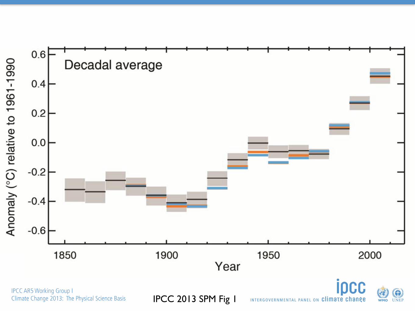
Figure SPM.1 [FIGURE SUBJECT TO FINAL COPYEDIT]
Twelfth Session of Working Group I Approved Summary for Policymakers
IPCC WGI AR5 SPM-27 27 September 2013
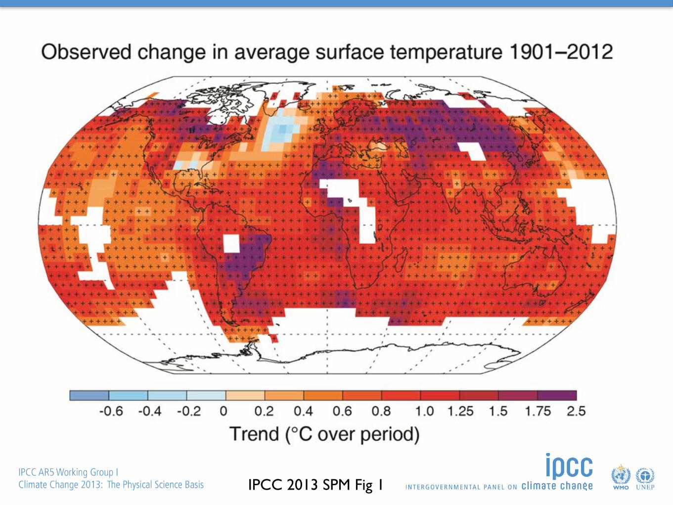
Figure SPM.1 [FIGURE SUBJECT TO FINAL COPYEDIT]
IPCC 2013 SPM Fig 1
Twelfth Session of Working Group I Approved Summary for Policymakers
IPCC WGI AR5 SPM-27 27 September 2013
Figure SPM.1 [FIGURE SUBJECT TO FINAL COPYEDIT]
IPCC 2013 SPM Fig 1
Final Draft (7 June 2013) Chapter 2 IPCC WGI Fifth Assessment Report
Do Not Cite, Quote or Distribute 2-145 Total pages: 163
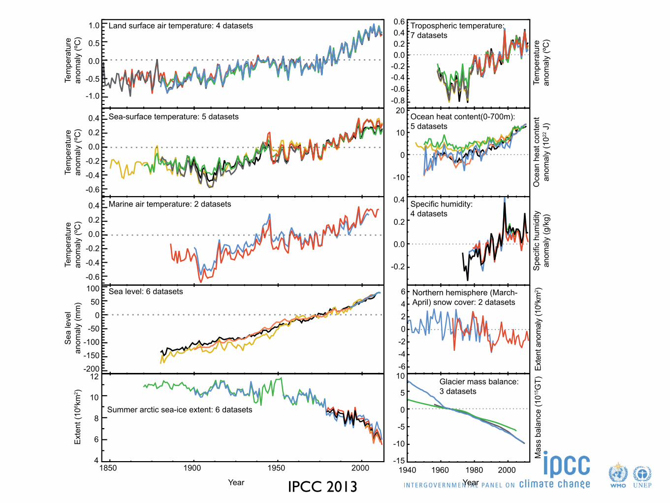
FAQ 2.1, Figure 2: Multiple independent indicators of a changing global climate. Each line represents an independently-derived estimate of change in the climate element. In each panel all datasets have been normalized to a common period of record. A full detailing of which source datasets go into which panel is given in the Supplementary Material 2.SM.5.
Land surface air temperature: 4 datasets
Mas
s ba
lanc
e (1
015G
T)
1.0
0.5
0.0
-0.5
-1.0
0.4
0.2
0.0
-0.2
-0.4
-0.6
0.4
0.2
0.0
-0.2
-0.4
-0.6
12
10
8
6
4
10
5
0
-5
-10
-15
0.4
0.2
0.0
-0.2
20
10
0
-10
0.60.40.20.0
-0.2-0.4-0.6-0.8
10050
0-50
-100-150-200
Tropospheric temperature:7 datasets
Ocean heat content(0-700m):5 datasets
Specific humidity:4 datasets
Glacier mass balance:3 datasets
Sea-surface temperature: 5 datasets
Marine air temperature: 2 datasets
Sea level: 6 datasets
1850 1900 1950 2000 1940 1960 1980 2000
Summer arctic sea-ice extent: 6 datasets
Sea
leve
lan
omal
y (m
m)
Tem
pera
ture
anom
aly
(ºC
)Te
mpe
ratu
rean
omal
y (º
C)
Tem
pera
ture
anom
aly
(ºC
)
Tem
pera
ture
anom
aly
(ºC
)O
cean
hea
t con
tent
anom
aly
(1022
J)
Spec
ific
hum
idity
anom
aly
(g/k
g)Ex
tent
ano
mal
y (1
06 km
2 )6420
-2-4-6
Exte
nt (1
06 km
2 )
Year Year
Northern hemisphere (March-April) snow cover: 2 datasets
IPCC 2013
1920 1940 1960 1980 2000 2020Year
-6-4
-2
0
2
4
6
SCE
anom
aly
(106 s
q. k
m)
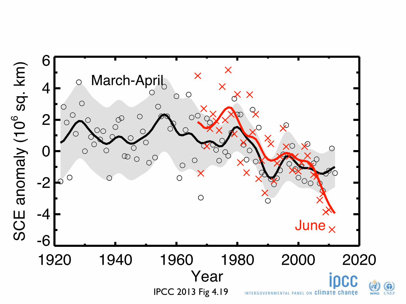
March-April
June
IPCC 2013 Fig 4.19
Headline statementsHuman influence on the climate system is clear... [and] has been detected in warming of the atmosphere and the ocean, in changes in the global water cycle, in reductions in snow and ice, in global mean sea level rise, and in changes in some climate extremes. ... It is extremely likely that human influence has been the dominant cause of the observed warming since the mid-20th century.
Twelfth Session of Working Group I Approved Summary for Policymakers
IPCC WGI AR5 SPM-32 27 September 2013
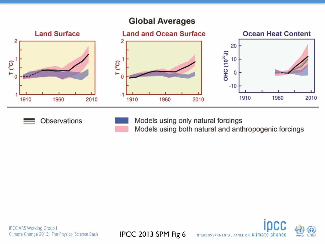
Figure SPM.6 [FIGURE SUBJECT TO FINAL COPYEDIT]
IPCC 2013 SPM Fig 6
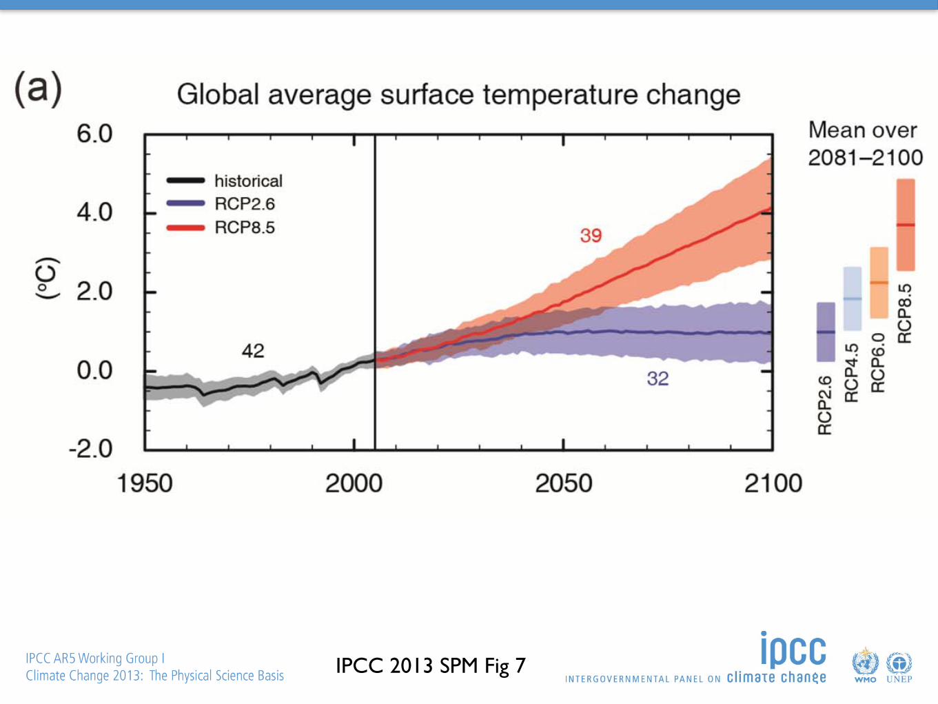
Headline statementsGlobal surface temperature change for the end of the 21st century is likely to exceed 1.5°C relative to 1850 to 1900 for all RCP scenarios except RCP2.6.
Final Draft (7 June 2013) Chapter 1 IPCC WGI Fifth Assessment Report
Do Not Cite, Quote or Distribute 1-46 Total pages: 62
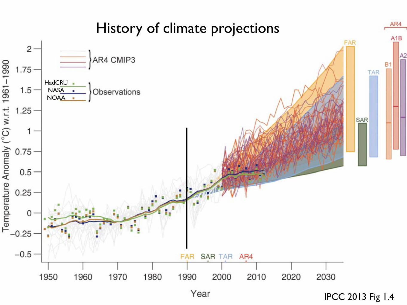
Figure 1.4: Estimated changes in the observed globally and annually averaged surface temperature anomaly relative to 1961–1990 (in qC) since 1950 compared with the range of projections from the previous IPCC assessments. Values are harmonized to start from the same value in 1990. Observed global annual mean surface air temperature anomaly, relative to 1961–1990, is shown as squares and smoothed time series as solid lines (NASA (dark blue), NOAA (warm mustard), and the UK Hadley Centre (bright green) reanalyses). The coloured shading shows the projected range of global annual mean surface air temperature change from 1990 to 2035 for models used in FAR (Figure 6.11 in Bretherton et al., 1990), SAR (Figure 19 in the TS of IPCC, 1996), TAR (full range of TAR Figure 9.13(b) in Cubasch et al., 2001). TAR results are based on the simple climate model analyses presented and not on the individual full three-dimensional climate model simulations. For the AR4 results are presented as single model runs of the CMIP3 ensemble for the historical period from 1950 to 2000 (light grey lines) and for three scenarios (A2, A1B and B1) from 2001 to 2035. The bars at the right hand side of the graph show the full range given for 2035 for each assessment report. For the three SRES scenarios the bars show the CMIP3 ensemble mean and the likely range given by –40% to +60% of the mean as assessed in Meehl et al. (2007). The publication years of the assessment reports are shown. See Appendix 1.A for details on the data and calculations used to create this figure.
IPCC 2013 Fig 1.4
History of climate projections
HadCRUNASANOAA
Twelfth Session of Working Group I Approved Summary for Policymakers
IPCC WGI AR5 SPM-33 27 September 2013
Figure SPM.7 [FIGURE SUBJECT TO FINAL COPYEDIT]
IPCC 2013 SPM Fig 7
Twelfth Session of Working Group I Approved Summary for Policymakers
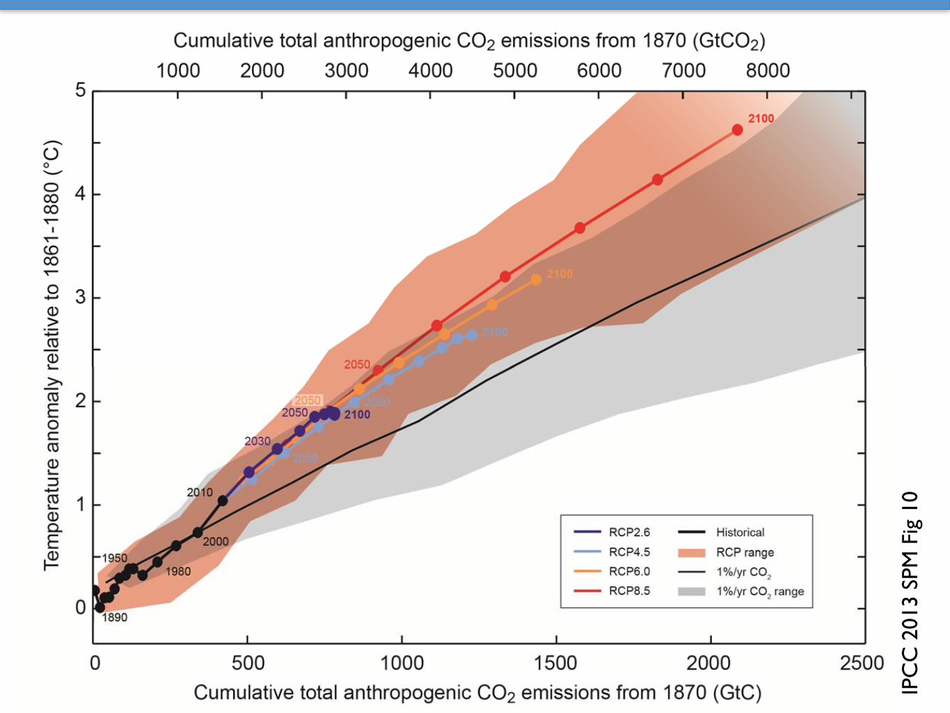
IPCC WGI AR5 SPM-36 27 September 2013
Figure SPM.10 [FIGURE SUBJECT TO FINAL COPYEDIT]
]
IPC
C 2
013
SPM
Fig
10
Outline
• 1 slide of climate science
• Background, scope, and processes of IPCC
• Summary of main results
• Observed changes in extremes
• the global warming ‘hiatus’
• Changes in ENSO etc.
Final Draft (7 June 2013) Chapter 2 IPCC WGI Fifth Assessment Report
Do Not Cite, Quote or Distribute 2-150 Total pages: 163
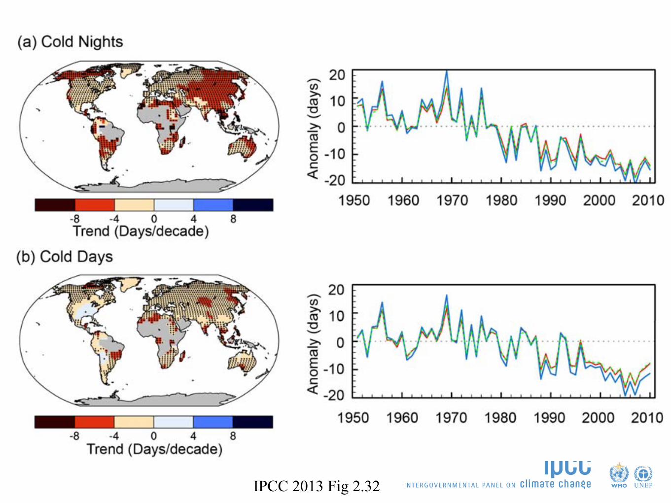
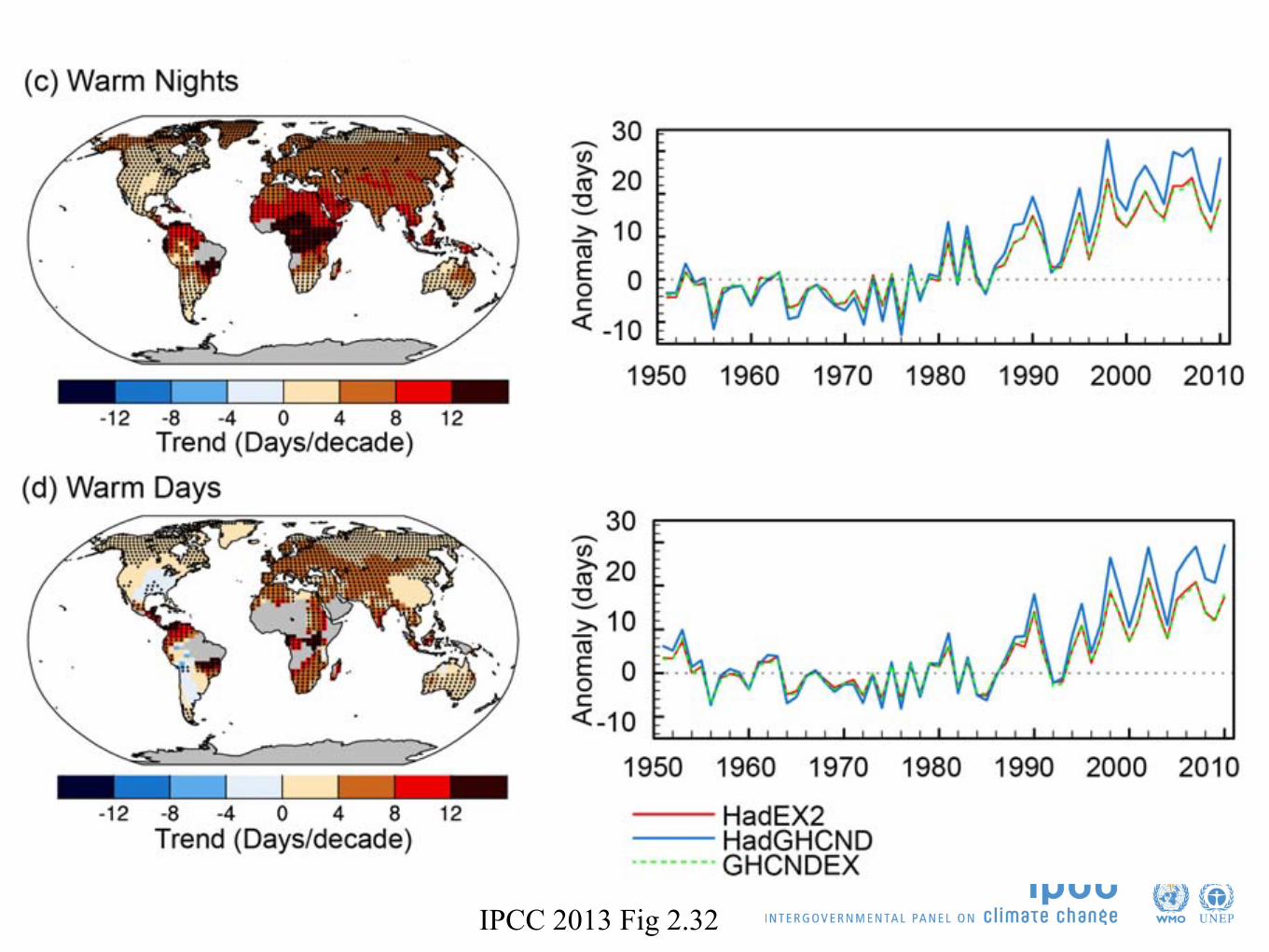
Figure 2.32: Trends in annual frequency of extreme temperatures over the period 1951–2010, for: (a) cold nights (TN10p), (b) cold days (TX10p), (c) warm nights (TN90p) and (d) warm days (TX90p) (Box 2.4, Table 1). Trends were calculated only for grid boxes that had at least 40 years of data during this period and where data ended no earlier than 2003. Grey areas indicate incomplete or missing data. Black plus signs (+) indicate grid boxes where trends are significant (i.e., a trend of zero lies outside the 90% confidence interval). The data source for trend maps is HadEX2 (Donat et al., 2013c) updated to include the latest version of the European Climate Assessment dataset (Klok and Tank, 2009). Beside each map are the near-global time series of annual anomalies of these indices with respect to 1961–1990 for three global indices datasets: HadEX2 (red); HadGHCND (Caesar et al., 2006; blue) and updated to 2010 and GHCNDEX (Donat et al., 2013a; green). Global averages are only calculated using grid boxes where all three datasets have at least 90% of data over the time period. Trends are significant (i.e., a trend of zero lies outside the 90% confidence interval) for all the global indices shown.
IPCC 2013 Fig 2.32
Final Draft (7 June 2013) Chapter 2 IPCC WGI Fifth Assessment Report
Do Not Cite, Quote or Distribute 2-150 Total pages: 163
Figure 2.32: Trends in annual frequency of extreme temperatures over the period 1951–2010, for: (a) cold nights (TN10p), (b) cold days (TX10p), (c) warm nights (TN90p) and (d) warm days (TX90p) (Box 2.4, Table 1). Trends were calculated only for grid boxes that had at least 40 years of data during this period and where data ended no earlier than 2003. Grey areas indicate incomplete or missing data. Black plus signs (+) indicate grid boxes where trends are significant (i.e., a trend of zero lies outside the 90% confidence interval). The data source for trend maps is HadEX2 (Donat et al., 2013c) updated to include the latest version of the European Climate Assessment dataset (Klok and Tank, 2009). Beside each map are the near-global time series of annual anomalies of these indices with respect to 1961–1990 for three global indices datasets: HadEX2 (red); HadGHCND (Caesar et al., 2006; blue) and updated to 2010 and GHCNDEX (Donat et al., 2013a; green). Global averages are only calculated using grid boxes where all three datasets have at least 90% of data over the time period. Trends are significant (i.e., a trend of zero lies outside the 90% confidence interval) for all the global indices shown.
IPCC 2013 Fig 2.32
The ‘Hiatus’
• Depends on starting point: 1998 very warm
• 1998-2012 still positive: 0.04°C
• Consistent with internal variability, observed radiative forcing, increased ocean heat flux
Box TS.3
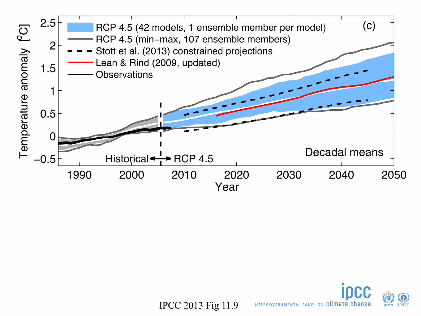
Final Draft (7 June 2013) Chapter 11 IPCC WGI Fifth Assessment Report
Do Not Cite, Quote or Distribute 11-102 Total pages: 123
Figure 11.9: a) Projections of global mean, annual mean surface air temperature 1986–2050 (anomalies relative to 1986–2005) under RCP4.5 from CMIP5 models (blue lines, one ensemble member per model), with four observational estimates (HadCRUT3: Brohan et al. (2006); ERA-Interim: Simmons et al. (2010); GISTEMP: Hansen et al., 2010; NOAA: Smith et al. (2008) for the period 1986–2011 (black lines); b) as in a) but showing the 5–95% range (grey and blue shades, with the multi-model median in white) of annual mean CMIP5 projections using one ensemble member per model from RCP4.5 scenario, and annual mean observational estimates (solid black line). The maximum and minimum values from CMIP5 are shown by the grey lines. Red hatching shows 5–95% range for predictions initialized in 2006 for 14 CMIP5 models applying the Meehl and Teng (2012) methodology. Black hatching shows the 5–95% range for predictions initialized in 2011 for 8 models from Smith et al. (2013b). c) as a) but showing the 5–95% range (grey and blue shades, with the multi-model median in white) of decadal mean CMIP5 projections using one ensemble member per model from RCP4.5 scenario, and decadal mean observational estimates (solid black line). The maximum and minimum values from CMIP5 are shown by the grey lines. The dashed black lines show an estimate of the projected 5–95% range for decadal mean global mean surface air temperature for the period 2016–2040 derived using the ASK methodology applied to 6 CMIP5 GCMs (from Stott et al. (2013). The red line shows a statistical prediction based on the method of Lean and Rind (2009), updated for RCP4.5.
IPCC 2013 Fig 11.9
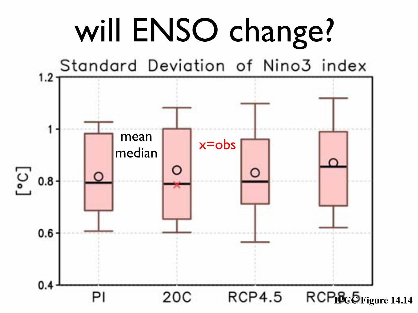
will ENSO change?Final Draft (7 June 2013) Chapter 14 IPCC WGI Fifth Assessment Report
Do Not Cite, Quote or Distribute 14-129 Total pages: 145
Figure 14.14: Standard deviation of Niño3 SST anomalies from CMIP5 model experiments. PI, 20C, RCP4.5, RCP8.5
indicate pre-industrial control experiments, 20th century experiments, and 21st century experiment from the RCP4.5
and RCP8.5. Open dot and solid black line indicate multi-model ensemble mean and median, respectively, and the cross
mark is 20th observation, respectively. Thick bar and thin outer bar indicate 50% and 75% percentile ranges,
respectively.
IPCC Figure 14.14
x=obsmeanmedian
Conclusions
• “Warming of the climate system is unequivocal”
• “...human influence has been the dominant cause of the observed warming...”
© Yann Arthus-Bertrand / Altitude
www.climatechange2013.orgFurther Information
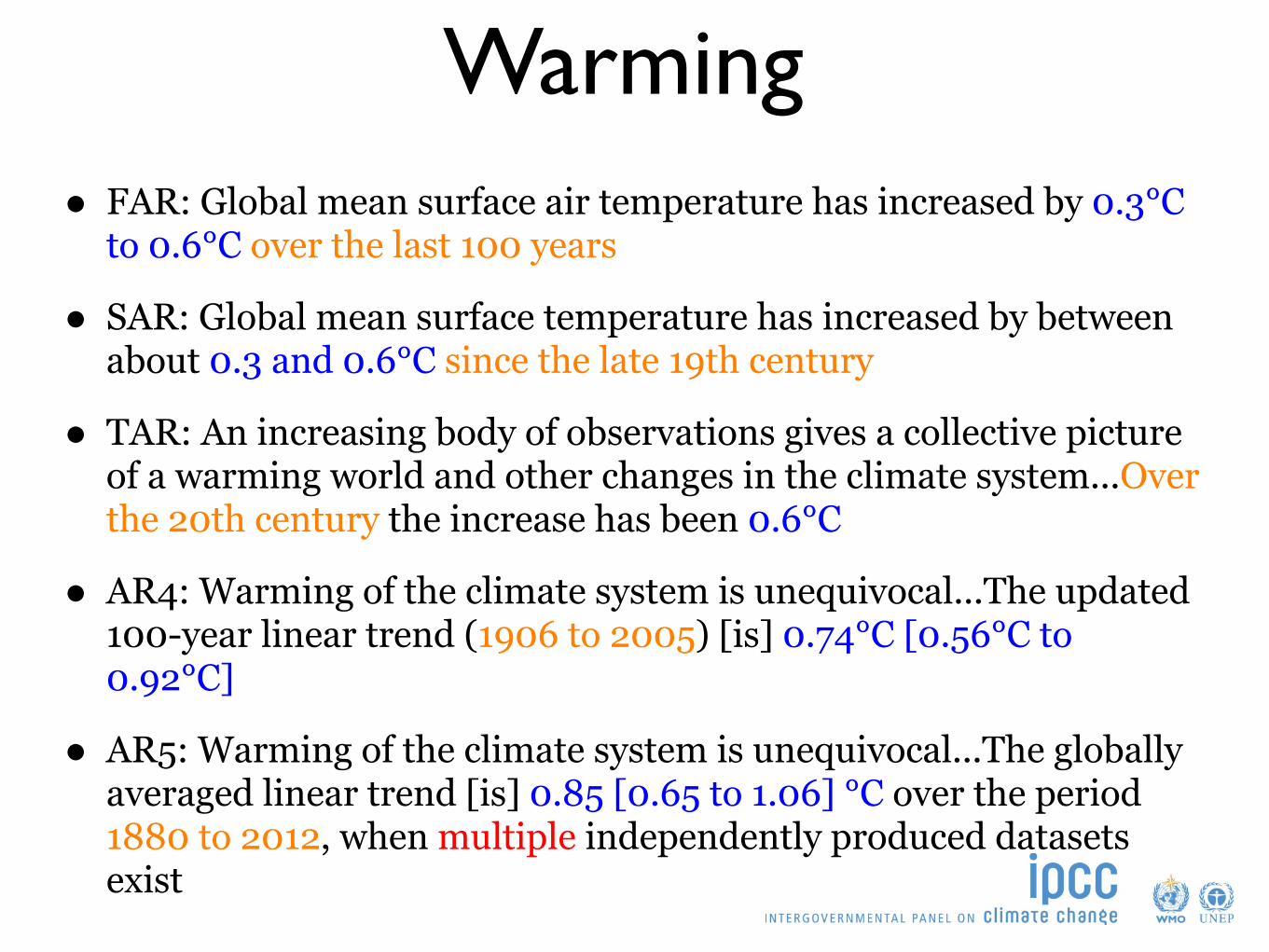
Warming• FAR: Global mean surface air temperature has increased by 0.3°C
to 0.6°C over the last 100 years
• SAR: Global mean surface temperature has increased by between about 0.3 and 0.6°C since the late 19th century
• TAR: An increasing body of observations gives a collective picture of a warming world and other changes in the climate system...Over the 20th century the increase has been 0.6°C
• AR4: Warming of the climate system is unequivocal...The updated 100-year linear trend (1906 to 2005) [is] 0.74°C [0.56°C to 0.92°C]
• AR5: Warming of the climate system is unequivocal...The globally averaged linear trend [is] 0.85 [0.65 to 1.06] °C over the period 1880 to 2012, when multiple independently produced datasets exist
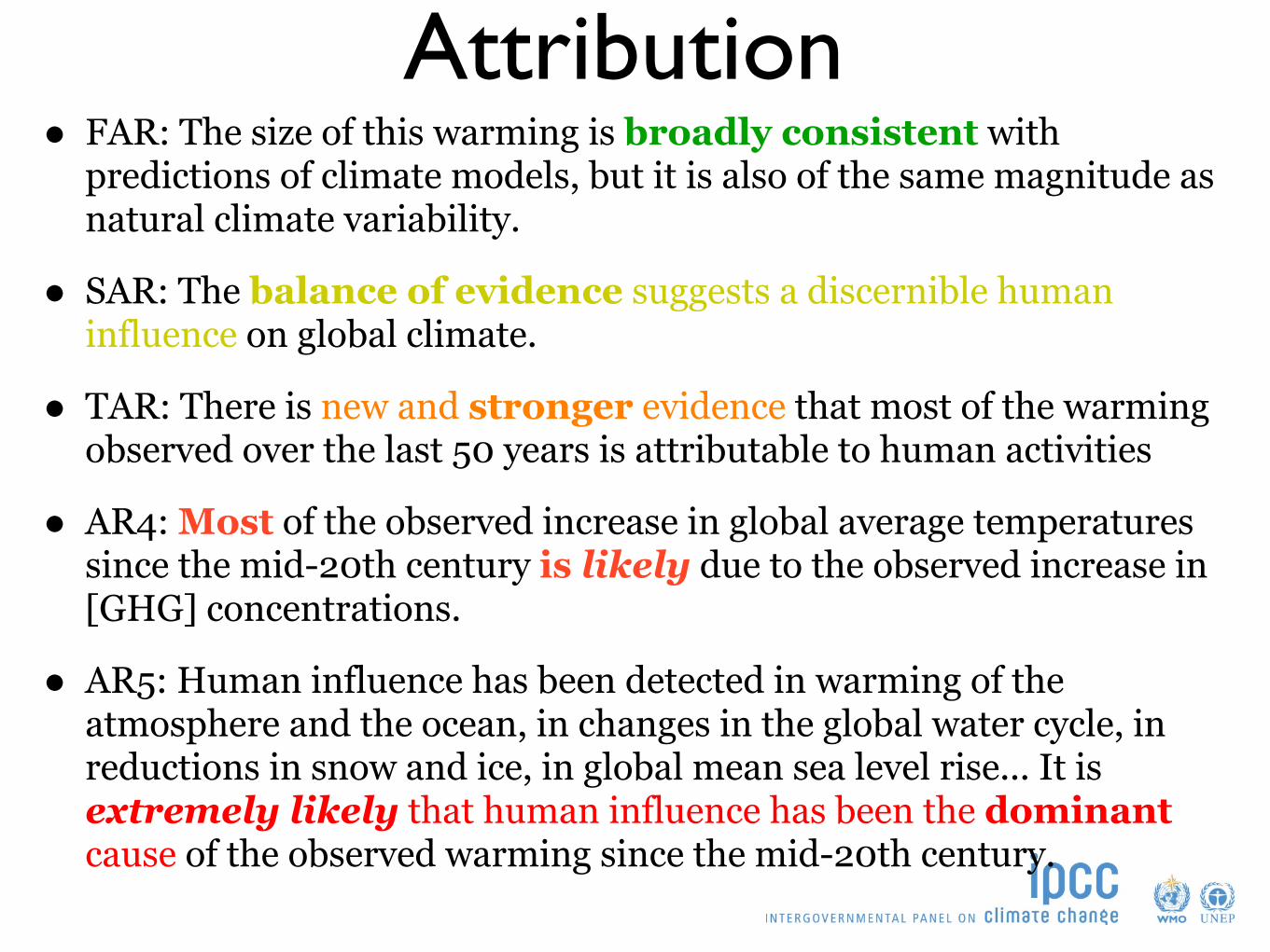
Attribution• FAR: The size of this warming is broadly consistent with
predictions of climate models, but it is also of the same magnitude as natural climate variability.
• SAR: The balance of evidence suggests a discernible human influence on global climate.
• TAR: There is new and stronger evidence that most of the warming observed over the last 50 years is attributable to human activities
• AR4: Most of the observed increase in global average temperatures since the mid-20th century is likely due to the observed increase in [GHG] concentrations.
• AR5: Human influence has been detected in warming of the atmosphere and the ocean, in changes in the global water cycle, in reductions in snow and ice, in global mean sea level rise... It is extremely likely that human influence has been the dominant cause of the observed warming since the mid-20th century.
Final Draft (7 June 2013) Chapter 1 IPCC WGI Fifth Assessment Report
Do Not Cite, Quote or Distribute 1-52 Total pages: 62
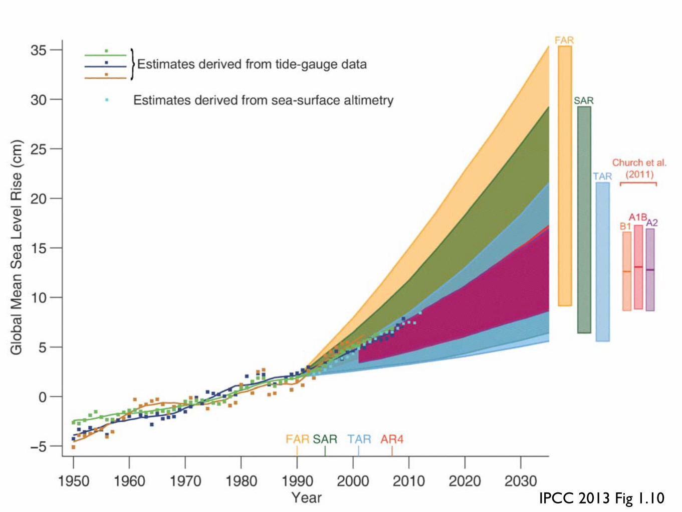
Figure 1.10: Estimated changes in the observed global annual mean sea level (GMSL) since 1950 relative to 1961–1990. Estimated changes in global annual sea level anomalies are presented based on tide gauge data (Church and White, 2011 (dark blue); Jevrejeva et al., 2008 (warm mustard) ; Ray and Douglas, 2011 (dark green)) and based on sea surface altimetry (light blue). The altimetry data start in 1993 and are harmonized to start from the mean 1993 value of the tide gauge data. Squares indicate annual mean values, solid lines smoothed values. The shading shows the largest model projected range of global annual sea level rise from 1950 to 2035 for FAR (Figure 9.6 and Figure 9.7 in Warrick and Oerlemans, 1990), SAR (Figure 21 in TS of IPCC, 1996), TAR (Appendix II of IPCC, 2001) and for Church et al. (2011) based on the Coupled Model Intercomparison Project Phase 3 (CMIP3) model results not assessed at the time of AR4 using the SRES B1, A1B, and A2 scenarios. Note that in the AR4 no full range was given for the sea level projections for this period. Therefore, the figure shows results that have been published subsequent to the AR4. The bars at the right hand side of the graph show the full range given for 2035 for each assessment report. For Church et al. (2011) the mean sea level rise is indicated in addition to the full range. See Appendix 1.A for details on the data and calculations used to create this figure.
IPCC 2013 Fig 1.10
Final Draft (7 June 2013) Chapter 2 IPCC WGI Fifth Assessment Report
Do Not Cite, Quote or Distribute 2-118 Total pages: 163
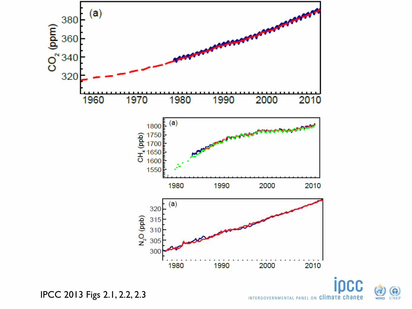
Figure 2.3: a) Globally averaged N2O dry-air mole fractions from AGAGE (red) and NOAA/ESRL/GMD (blue) at monthly resolution. b) Instantaneous growth rates for globally averaged atmospheric N2O. Growth rates were calculated as in Figure 2.1.
Final Draft (7 June 2013) Chapter 2 IPCC WGI Fifth Assessment Report
Do Not Cite, Quote or Distribute 2-117 Total pages: 163
Figure 2.2: a) Globally averaged CH4 dry-air mole fractions from UCI (green; 4 values per year, except prior to 1984,
when they are of lower and varying frequency), AGAGE (red; monthly), and NOAA/ESRL/GMD (blue; quasi-weekly).
b) Instantaneous growth rate for globally averaged atmospheric CH4 using the same colour code as in (a). Growth rates
were calculated as in Figure 2.1.
Final Draft (7 June 2013) Chapter 2 IPCC WGI Fifth Assessment Report
Do Not Cite, Quote or Distribute 2-116 Total pages: 163
Figures
Figure 2.1: a) Globally averaged CO2 dry-air mole fractions from Scripps Institution of Oceanography (SIO) at
monthly time resolution based on measurements from Mauna Loa, Hawaii and South Pole (red) and
NOAA/ESRL/GMD at quasi-weekly time resolution (blue). SIO values are deseasonalized. b) Instantaneous growth
rates for globally averaged atmospheric CO2 using the same colour code as in (a). Growth rates are calculated as the
time derivative of the deseasonalized global averages (Dlugokencky et al., 1994).
Final Draft (7 June 2013) Chapter 2 IPCC WGI Fifth Assessment Report
Do Not Cite, Quote or Distribute 2-117 Total pages: 163
Figure 2.2: a) Globally averaged CH4 dry-air mole fractions from UCI (green; 4 values per year, except prior to 1984,
when they are of lower and varying frequency), AGAGE (red; monthly), and NOAA/ESRL/GMD (blue; quasi-weekly).
b) Instantaneous growth rate for globally averaged atmospheric CH4 using the same colour code as in (a). Growth rates
were calculated as in Figure 2.1.
Final Draft (7 June 2013) Chapter 2 IPCC WGI Fifth Assessment Report
Do Not Cite, Quote or Distribute 2-117 Total pages: 163
Figure 2.2: a) Globally averaged CH4 dry-air mole fractions from UCI (green; 4 values per year, except prior to 1984,
when they are of lower and varying frequency), AGAGE (red; monthly), and NOAA/ESRL/GMD (blue; quasi-weekly).
b) Instantaneous growth rate for globally averaged atmospheric CH4 using the same colour code as in (a). Growth rates
were calculated as in Figure 2.1.
IPCC 2013 Figs 2.1, 2.2, 2.3
Final Draft (7 June 2013) Chapter 2 IPCC WGI Fifth Assessment Report
Do Not Cite, Quote or Distribute 2-143 Total pages: 163
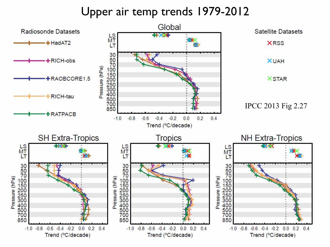
Figure 2.27: As Figure 2.26 except for the satellite era 1979–2012 period and including MSU products (RSS, STAR and UAH).
Upper air temp trends 1979-2012
IPCC 2013 Fig 2.27
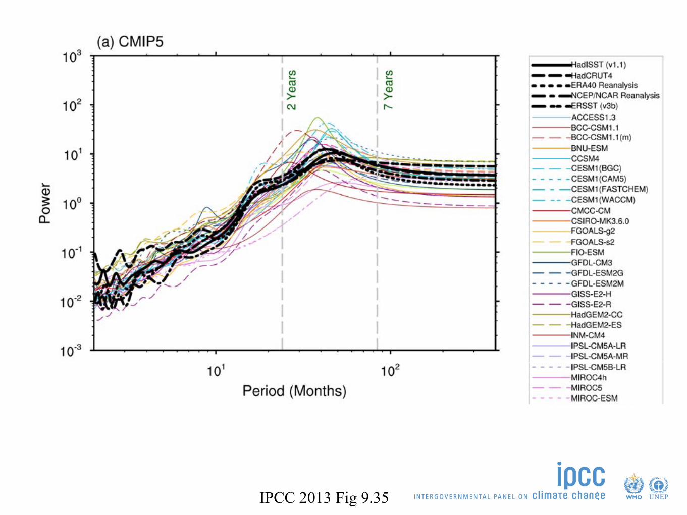
Final Draft (7 June 2013) Chapter 9 IPCC WGI Fifth Assessment Report
Do Not Cite, Quote or Distribute 9-191 Total pages: 205
Figure 9.35: Maximum entropy power spectra of surface air temperature averaged over the NINO3 region (5°N to 5°S, 150°W to 90°W) for (a) the CMIP5 models and (b) the CMIP3 models. ECMWF reanalysis in (a) refers to the European Centre for Medium Range Weather Forecasts (ECMWF) 15-year reanalysis (ERA15). The vertical lines correspond to periods of two and seven years. The power spectra from the reanalyses and for SST from the Hadley Centre Sea Ice and Sea Surface Temperature (HadISST) version 1.1, HadCRU 4, ERA40 and NCEP/NCAR data set are given by the series of black curves. Adapted from (AchutaRao and Sperber, 2006).
IPCC 2013 Fig 9.35