phenotypic evolution - indiana university bloomingtong562/lectures/lecture 11 - evolution and... ·...

Department of Geological Sciences | Indiana University (c) 2012, P. David Polly

G562 Geometric Morphometrics

and phylogenetic comparative methodsPhenotypic Evolution



Phenotypic EvolutionChange in the mean phenotype from generation to generation...

Evolution = Mean(genetic variation * selection) + Mean(genetic variation * drift) +

Mean(nongenetic variation)



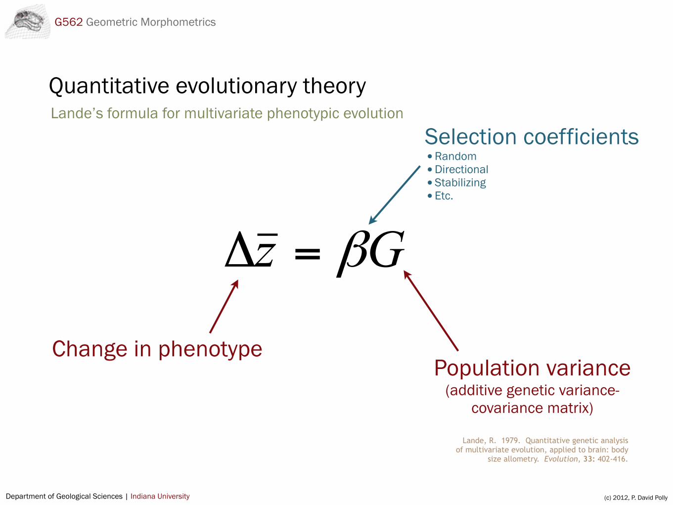
Quantitative evolutionary theory

Gz β=Δ

Change in phenotype

Lande’s formula for multivariate phenotypic evolution

Population variance(additive genetic variance-

covariance matrix)

Selection coefficients•Random•Directional•Stabilizing•Etc.

Lande, R. 1979. Quantitative genetic analysis of multivariate evolution, applied to brain: body

size allometry. Evolution, 33: 402-416.



Brown, W.M., M. George, Jr., & A.C. Wilson. 1979. Rapid evolution of animal mitochondrial DNA. PNAS, 76: 1967-1971.

Phenotypic trait divergence less predictable than genetic divergence

Mitochondrial DNA divergence

Polly, P.D. 2003. Paleophylogeography: the tempo of geographic differentiation in marmots (Marmota). Journal of

Mammalogy, 84: 369-384.

Molar shape divergence



Monte Carlo simulation of Brownian Motion properties

“Monte Carlo” is a type of modelling in which you simulate random samples of variables or systems of interest. Here we simulate 1000 random walks to see whether it is true that the average outcome is the same as the starting point and whether the variance and standard deviation of outcomes occur as expected.

walks = Table[RandomWalk[100, 1], {1000}];ListPlot[walks, Joined -> True, Axes -> False, Frame -> True, PlotRange -> All]Histogram[walks[[1 ;;, -1]], Axes -> False]Mean[walks[[1;;, -1]]]Variance[walks[[1;;,-1]]]StandardDeviation[walks[[1;;,-1]]]



Random walks

1 random walk 100 random walks



Statistics of Brownian motion evolution“Random walk” evolution:

1. Change at each generation is random in direction and magnitude

2. Direction of change at any point does not depend on previous changes

Consequently....

3. The most likely endpoint is the starting point

4. The distribution of possible endpoints has a variance that equals the average squared change per generation * number of generations

5. The standard deviation of possible endpoints increases with the square root of number ofgenerations



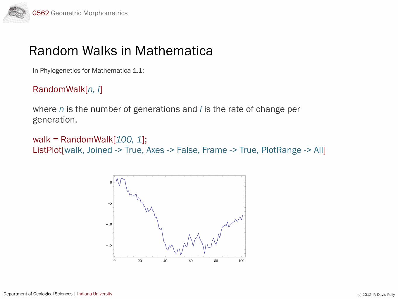
Random Walks in MathematicaIn Phylogenetics for Mathematica 1.1:

RandomWalk[n, i]

where n is the number of generations and i is the rate of change per generation.

walk = RandomWalk[100, 1];ListPlot[walk, Joined -> True, Axes -> False, Frame -> True, PlotRange -> All]

0 20 40 60 80 100

-15

-10

-5

0



Results of Monte Carlo experiment100 generations, rate of 1.0 per generation, squared rate of 1.0 per generation, 10,000 runs

Expected Observed

Mean = 0 Mean = 0.034

Variance = 1.02 * 100 =100 Variance = 100.37

SD = Sqrt[1.02 * 100] =10 SD = 10.10



Two ways to think about phenotypic evolution

Phenotype graphs(phenotypic value over time)

Divergence graphs(phenotypic change over time)



Divergence graphs

Plots of divergence against phylogenetic, genetic, or geographic distance

Phylogenetic or Genetic Distance (time elapsed)

Mop

hom

etric

Div

erge

nce

(Pro

crus

tes

dist

ance

)

Each data point records the differences (morphological and phylogenetic) between two taxa (known as pairwise distances)



Divergence

Divergence

(2x)

Difference

Difference

Polly, P.D. 2001. Paleontology and the comparative method: ancestral node reconstructions versus observed node values.

American Naturalist, 157: 596-609.

Divergence graphs can be constructed from phylogenetic data



0 20 40 60 80 1000

5

10

15

20

25

Monte Carlo with Divergence GraphListPlot[Sqrt[walks^2], Joined -> True, Axes -> False, Frame -> True, PlotRange -> All]



How does one model evolution of shape?

Random walks of landmark coordinates are not realistic because the landmarks are highly correlated in real shapes.

Polly, P. D. 2004. On the simulation of the evolution of morphological shape: multivariate shape under selection and

drift. Palaeontologia Electronica, 7.2.7A: 28pp, 2.3MB. http://palaeo-electronica.org/paleo/2004_2/evo/issue2_04.htm

http://palaeo-electronica.org/paleo/2004_2/evo/issue2_04.htm






Shape evolution can be simulated in morphospaceThis approach takes covariances in landmarks into account

1. Collect landmarks, calculate covariance matrix2. Convert covariance matrix to one without correlations by rotating data to principal components3. Perform simulation in shape space, convert simulated scores back into landmark shape models



1 million generations of random selection100 lineages, 18 dimensional trait

Arrangement of cusps (red dots at right)

Positions of 100 lineages in first two dimensions of

morphospaceDivergence graph of 100 lineages









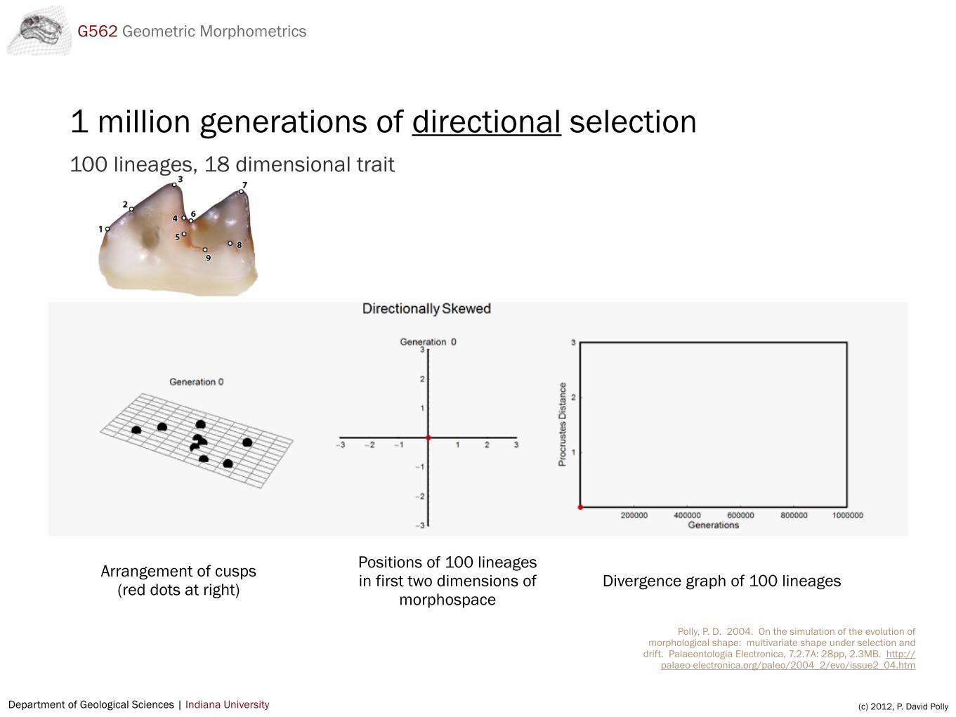
1 million generations of directional selection100 lineages, 18 dimensional trait












1 million generations of stabilizing selection100 lineages, 18 dimensional trait












BackgroundForward: landmarks to scores in shape space

proc = Procrustes[landmarks, 10, 2];consensus = Mean[proc];resids = # - consensus &/@proc;CM = Covariance[resids];{eigenvectors, v, w} = SingularValueDecomposition[CM];eigenvalues = Tr[v, List];

scores = resids.eigenvectors;

Backward: scores in shape space to landmarks

resids = scores.Transpose[eigenvectors];

proc = # + consensus &/@ resids;



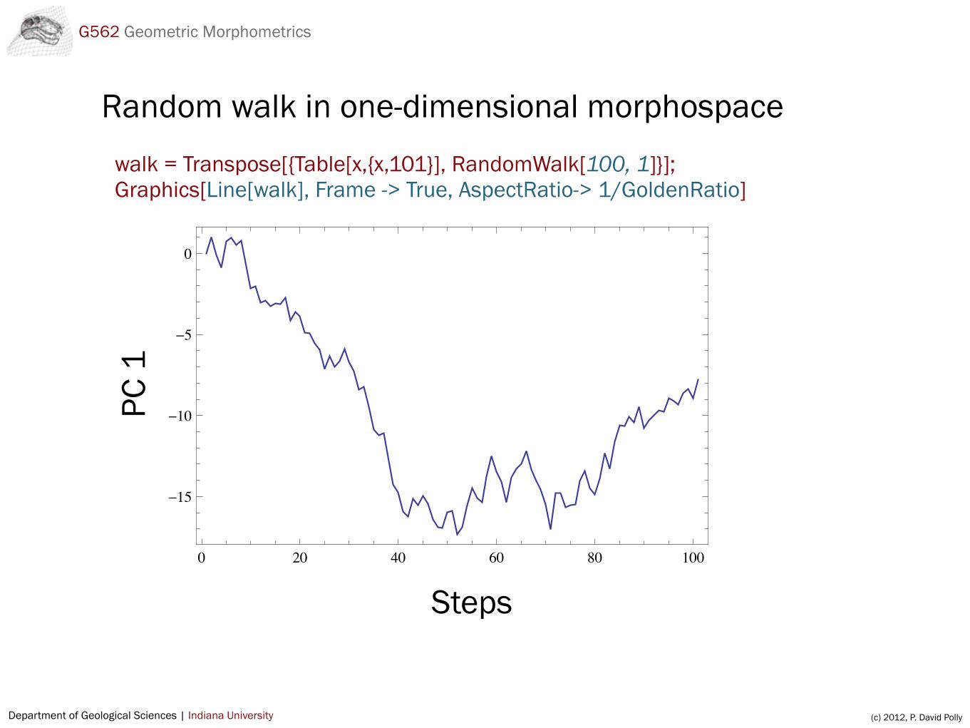
Random walk in one-dimensional morphospace

0 20 40 60 80 100

-15

-10

-5

0

Steps

PC 1

walk = Transpose[{Table[x,{x,101}], RandomWalk[100, 1]}];Graphics[Line[walk], Frame -> True, AspectRatio-> 1/GoldenRatio]



Random walk in two dimensions of shape space

Steps PC1

PC2

z1=0; z2=0;

walk2d = Table[{t,z1=z1+Random[NormalDistribution[0,1], z2=z2+Random[NormalDistribution[0,1]},{t,100}];Graphics3D[Line[walk2d]]



Same 2D random walk shown in two dimensionsz1=0; z2=0;

walk2d = Table[{z1=z1+Random[NormalDistribution[0,1], z2=z2+Random[NormalDistribution[0,1]},{t,100}];Graphics3D[Line[walk2d]]

0 5 10 15 20

-15

-10

-5

0

PC1

PC2



What rate to choose?

WALLABY

LEOPARDHUMAN

OTTER

FOSSA

DOG

Node 0

Node 1

Node 2

Node 3

Node 4

-0.3 -0.2 -0.1 0.0 0.1 0.2 0.3 0.4

-0.15

-0.10

-0.05

0.00

0.05

0.10

0.15

PC 1

PC2

Variance = Eigenvalues

Variance of random walk = rate2 * number of stepsrate = Sqrt[Eigenvalues / number of steps]



Monte carlo simulation of evolving turtlesturtlespace = Graphics[{PointSize[0.02], Black, Point[scores[[1 ;;, {1, 2}]]]}, AspectRatio -> Automatic, Frame -> True]

-0.05 0.00 0.05

-0.04

-0.02

0.00

0.02

0.04



Monte carlo simulation of evolving turtlesrates = Sqrt[eigvals[[1 ;; 2]]/100];

walk2d = Transpose[Table[RandomWalk[100, rates[[x]]], {x, Length[rates]}]];

Show[Graphics[{Gray, Line[walk2d]}, Frame -> True], turtlespace, PlotRange -> All]

-0.10 -0.05 0.00 0.05 0.10

-0.04

-0.02

0.00

0.02

0.04



Animated turtle evolutionListAnimate[Table[tpSpline[consensus, (walk2d[[x]].(Transpose[eigenvectors][[1 ;; 2]])) + consensus], {x, Length[walk2d]}]]



Important notes

•These simulations are based on the covariances of the taxa, not the covariances of a single population. Therefore they are not a true model of the evolution of a population by means of random selection.

•The rates used in this simulation are estimated without taking into account phylogenetic relationships among the taxa. The rates estimated using the variance of the taxa will be approximately correct, but one might really want to estimate them by taking into account phylogenetic relationships (e.g., Martins and Hansen, 1993).



Reconstructing evolution of shapeBrownian motion in reverse

Most likely ancestral phenotype is same as descendant, variance in likelihood is proportional time since the ancestor lived

-20 -10 0 10 20

20

40

60

80

100

Descendant

Ancestor?



Ancestor of two branches on phylogenetic tree

If likelihood of ancestor of one descendant is normal distribution with variance proportional to time, then likelihood of two ancestors is the product of their probabilities.

This is the maximum likelihood method for estimating phylogeny, and for reconstructing ancestral phenotypes. (Felsenstein,

Descendant 2

Common ancestor?

Descendant 1



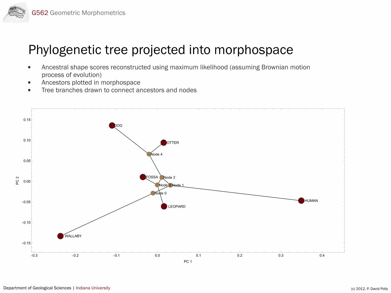
Phylogenetic tree projected into morphospace

WALLABY

LEOPARDHUMAN

OTTER

FOSSA

DOG

Node 0

Node 1

Node 2

Node 3

Node 4

-0.3 -0.2 -0.1 0.0 0.1 0.2 0.3 0.4

-0.15

-0.10

-0.05

0.00

0.05

0.10

0.15

PC 1

PC2

• Ancestral shape scores reconstructed using maximum likelihood (assuming Brownian motion process of evolution)

• Ancestors plotted in morphospace• Tree branches drawn to connect ancestors and nodes

Department of Geological Sciences | Indiana University(c) 2016, P. David Polly

Change in phenotype

Selection coefficients

Additive genetic variance – covariance matrix

Selection coefficients can be: Random Directional Stabilizing Etc.

Local Adaptive Peak

(selection on crown height

based on local conditions)Local Phenotype

(crown height in local population)

Mean

Variance

Op

tiu

mu

m

Peak Width

Direction of

Selection

Probability of extinction

Selection and drift: Lande’s adaptive peak model

Lande, R. 1976. Evolution, 30: 314-334.

• Selection vector = proportional to log slope of adaptive peak at population mean• Extirpation probability = chance event with probability that increases with distance from optimum• Genetic variance = population variance times heritability• Drift (not shown) = chance sampling based on heritable phenotypic variance and local population size

Parameters

Note: each geographic cell in the simulation has its own adaptive peak. Selection acts on local populations, not entire species.



Evolution on an adaptive landscape

Loosely following Lande (1976)…

Lande, R. 1976. Natural Selection and random genetic drift in phenotypic evolution. Evolution, 30: 314-334.

Δz = h2*σ2 * δ ln(W)/δz(t) z – mean phenotype h2 –heritability σ2 – phenotypic variance W – selective surface (adaptive landscape) δ – derivative (slope)



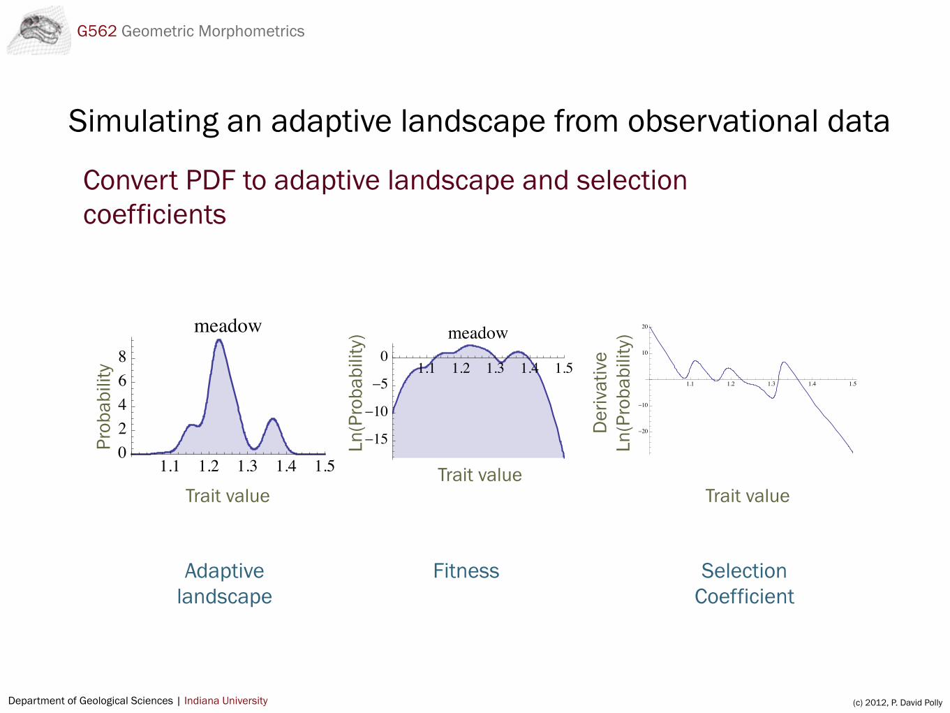
Simulating an adaptive landscape from observational data

Convert PDF to adaptive landscape and selection coefficients

1.1 1.2 1.3 1.4 1.502468

meadow

Trait value

Prob

abili

ty 1.1 1.2 1.3 1.4 1.5

-15

-10

-5

0meadow

Trait value

Ln(P

roba

bilit

y)

1.1 1.2 1.3 1.4 1.5

-20

-10

10

20

Trait value

Der

ivat

ive

Ln(P

roba

bilit

y)

Adaptive landscape

Fitness Selection Coefficient



Evolution on an adaptive landscape

Trait value

Time (generations)

phenotypic evolution - indiana university bloomingtong562/lectures/lecture 11 - evolution and... ·...

Documents