phase transitions a brief account with modern applications by gitterman and halpern
DESCRIPTION
Phase transitionTRANSCRIPT


PHASETRAMSITIOMS A Brief Account with
Modern Applications

This page intentionally left blank
PHASETRAMSITIOMS A Brief Account with
Modern Applications
Moshe Gitterrnan Vivian (Hairn) Halpern Bar-Ilan University, Israel
r p World Scientific N E W JERSEY LONDON SINGAPORE BElJ lNG S H A N G H A I HONG KONG TAIPEI CHENNAI

British Library Cataloguing-in-Publication DataA catalogue record for this book is available from the British Library.
For photocopying of material in this volume, please pay a copying fee through the CopyrightClearance Center, Inc., 222 Rosewood Drive, Danvers, MA 01923, USA. In this case permission tophotocopy is not required from the publisher.
ISBN 981-238-903-2
Typeset by Stallion PressEmail: [email protected]
All rights reserved. This book, or parts thereof, may not be reproduced in any form or by any means,electronic or mechanical, including photocopying, recording or any information storage and retrievalsystem now known or to be invented, without written permission from the Publisher.
Copyright © 2004 by World Scientific Publishing Co. Pte. Ltd.
Published by
World Scientific Publishing Co. Pte. Ltd.
5 Toh Tuck Link, Singapore 596224
USA office: 27 Warren Street, Suite 401–402, Hackensack, NJ 07601
UK office: 57 Shelton Street, Covent Garden, London WC2H 9HE
Printed in Singapore.
PHASE TRANSITIONSA Brief Account with Modern Applications

June 25, 2004 14:20 WSPC/Book Trim Size for 9in x 6in fm
Contents
Preface ix
1. Phases and Phase Transitions 1
1.1 Classification of Phase Transitions . . . . . . . . . . . 41.2 Appearance of a Second Order Phase Transition . . . 71.3 Correlations . . . . . . . . . . . . . . . . . . . . . . . . 91.4 Conclusion . . . . . . . . . . . . . . . . . . . . . . . . 11
2. The Ising Model 13
2.1 1D Ising model . . . . . . . . . . . . . . . . . . . . . . 162.2 2D Ising model . . . . . . . . . . . . . . . . . . . . . . 172.3 3D Ising model . . . . . . . . . . . . . . . . . . . . . . 202.4 Conclusion . . . . . . . . . . . . . . . . . . . . . . . . 23
3. Mean Field Theory 25
3.1 Landau Mean Field Theory . . . . . . . . . . . . . . . 263.2 First Order Phase Transitions in Landau Theory . . . 293.3 Landau Theory Supplemented with Fluctuations . . . 303.4 Critical Indices . . . . . . . . . . . . . . . . . . . . . . 323.5 Ginzburg Criterion . . . . . . . . . . . . . . . . . . . . 323.6 Wilson’s ε-Expansion . . . . . . . . . . . . . . . . . . . 333.7 Conclusion . . . . . . . . . . . . . . . . . . . . . . . . 36
v

June 25, 2004 14:20 WSPC/Book Trim Size for 9in x 6in fm
vi Phase Transition
4. Scaling 37
4.1 Relations Between Thermodynamic Critical Indices . . 394.2 Scaling Relations . . . . . . . . . . . . . . . . . . . . . 414.3 Dynamic Scaling . . . . . . . . . . . . . . . . . . . . . 454.4 Conclusion . . . . . . . . . . . . . . . . . . . . . . . . 47
5. The Renormalization Group 49
5.1 Fixed Points of a Map . . . . . . . . . . . . . . . . . . 495.2 Basic Idea of the Renormalization Group . . . . . . . 515.3 RG: 1D Ising Model . . . . . . . . . . . . . . . . . . . 535.4 RG: 2D Ising Model for the Square Lattice (1) . . . . 545.5 RG: 2D Ising Model for the Square Lattice (2) . . . . 575.6 Conclusion . . . . . . . . . . . . . . . . . . . . . . . . 60
6. Phase Transitions in Quantum Systems 63
6.1 Symmetry of the Wave Function . . . . . . . . . . . . 636.2 Exchange Interactions of Fermions . . . . . . . . . . . 656.3 Quantum Statistical Physics . . . . . . . . . . . . . . . 676.4 Superfluidity . . . . . . . . . . . . . . . . . . . . . . . 716.5 Bose–Einstein Condensation of Atoms . . . . . . . . . 726.6 Superconductivity . . . . . . . . . . . . . . . . . . . . 736.7 High Temperature (High-Tc) Superconductors . . . . . 786.8 Conclusion . . . . . . . . . . . . . . . . . . . . . . . . 80
7. Universality 81
7.1 Heisenberg Ferromagnet and Related Models . . . . . 817.2 Many-Spin Interactions . . . . . . . . . . . . . . . . . 857.3 Gaussian and Spherical Models . . . . . . . . . . . . . 867.4 The x–y Model . . . . . . . . . . . . . . . . . . . . . . 887.5 Vortices . . . . . . . . . . . . . . . . . . . . . . . . . . 927.6 Interactions Between Vortices . . . . . . . . . . . . . . 937.7 Vortices in Superfluids and Superconductors . . . . . . 957.8 Conclusion . . . . . . . . . . . . . . . . . . . . . . . . 96

June 25, 2004 14:20 WSPC/Book Trim Size for 9in x 6in fm
Contents vii
8. Random and Small World Systems 99
8.1 Percolation . . . . . . . . . . . . . . . . . . . . . . . . 998.2 Ising Model with Random Interactions . . . . . . . . . 1018.3 Spin Glasses . . . . . . . . . . . . . . . . . . . . . . . . 1038.4 Small World Systems . . . . . . . . . . . . . . . . . . . 1058.5 Evolving Graphs . . . . . . . . . . . . . . . . . . . . . 1098.6 Phase Transitions in Small World Systems . . . . . . . 1108.7 Conclusion . . . . . . . . . . . . . . . . . . . . . . . . 112
9. Self-Organized Criticality 113
9.1 Power Law Distributions . . . . . . . . . . . . . . . . . 1159.2 Sand Piles . . . . . . . . . . . . . . . . . . . . . . . . . 1179.3 Distribution of Links in Networks . . . . . . . . . . . . 1189.4 Dynamics of Networks . . . . . . . . . . . . . . . . . . 1209.5 Mean Field Analysis of Networks . . . . . . . . . . . . 1249.6 Hubs in Scale-Free Networks . . . . . . . . . . . . . . 1269.7 Conclusion . . . . . . . . . . . . . . . . . . . . . . . . 128
Bibliography 129
Index 133

This page intentionally left blank

June 25, 2004 14:20 WSPC/Book Trim Size for 9in x 6in fm
Preface
This book is based on a short graduate course given by one of us(M.G) at New York University and at Bar-Ilan University, Israel.The decision to publish these lectures as a book was made, aftersome doubts, for the following reason. The theory of phase transi-tions, with excellent agreement between theory and experiment, wasdeveloped some forty years ago culminating in Wilson’s Nobel prizeand the Wolf prize awarded to Kadanoff, Fisher and Wilson. In spiteof this, new books on phase transitions appear each year, and each ofthem starts with the justification of the need for an additional book.Following this tradition we would like to underline two main featuresthat distinguish this book from its predecessors.
Firstly, in addition to the five pillars of the modern theory ofphase transitions (Ising model, mean field, scaling, renormalizationgroup and universality) described in Chapters 2–5 and in Chapter 7,we have tried to describe somewhat more extensively those problemswhich are of major interest in modern statistical mechanics. Thus,in Chapter 6 we consider the superfluidity of helium and its connec-tion with the Bose–Einstein condensation of alkali atoms, and alsothe general theory of superconductivity and its relation to the hightemperature superconductors, while in Chapter 7 we treat the x–y
model associated with the theory of vortices in superconductors. Theshort description of percolation and of spin glasses in Chapter 8 iscomplemented by the presentation of the small world phenomena,which also involve short and long range order. Finally, we considerin Chapter 9 the applications of critical phenomena to self-organized
ix

June 25, 2004 14:20 WSPC/Book Trim Size for 9in x 6in fm
x Phase Transition
criticality in scale-free non-equilibrium systems. While each of thesetopics has been treated individually and in much greater detail indifferent books, we feel that there is a lot to be gained by presentingthem all together in a more elementary treatment which emphasizesthe connection between them. In line with this attempt to combinethe traditional, well-established issues with the recently publishedand not yet so widely known and more tentative topics, our fairlyshort list of references consists of two clearly distinguishable parts,one related to the classical theory of the sixties and seventies andthe other to the developments in the past few years. In the index, weonly list the pages where a topic is discussed in some detail, and ifthe discussion extends over more than one page then only the firstpage is listed.
We hope that simplicity and brevity are the second characteris-tic property of this book. We tried to avoid those problems whichrequire a deep knowledge of specialized topics in physics and math-ematics, and where this was unavoidable we brought the necessarydetails in the text. It is desirable these days that every scientist orengineer should be able to follow the new wide-ranging applicationsof statistical mechanics in science, economics and sociology. Accord-ingly, we hope that this short exposition of the modern theory ofphase transitions could usefully be a part of a course on statisticalphysics for chemists, biologists or engineers who have a basic knowl-edge of mathematics, statistical mechanics and quantum mechanics.Our book provides a basis for understanding current publications onthese topics in scientific periodicals. In addition, although studentsof physics who intend to do their own research will need more basicmaterial than is presented here, this book should provide them witha useful introduction to the subject and overview of it.
Mosh Gitterman & Vivian (Haim) HalpernJanuary 2004

June 25, 2004 14:17 WSPC/Book Trim Size for 9in x 6in chap01
Chapter 1
Phases and Phase Transitions
In discussing phase transitions, the first thing that we have to dois to define a phase. This is a concept from thermodynamics andstatistical mechanics, where a phase is defined as a homogeneoussystem. As a simple example, let us consider instant coffee. Thisconsists of coffee powder dissolved in water, and after stirring it wehave a homogeneous mixture, i.e., a single phase. If we add to a cupof coffee a spoonful of sugar and stir it well, we still have a singlephase — sweet coffee. However, if we add ten spoonfuls of sugar, thenthe contents of the cup will no longer be homogeneous, but rather amixture of two homogeneous systems or phases, sweet liquid coffeeon top and coffee-flavored wet sugar at the bottom.
In the above example, we obtained two different phases by chang-ing the composition of the system. However, the more usual type ofphase transition, and the one that we will consider mostly in thisbook, is when a single system changes its phase as a result of achange in the external conditions, such as temperature, pressure, oran external magnetic or electric field. The most familiar examplefrom everyday life is water. At room temperature and normal atmo-spheric pressure this is a liquid, but if its temperature is reduced tobelow 0C it will change into ice, a solid, while if its temperature israised to above 100C it will change into steam, a gas. As one variesboth the temperature and pressure, one finds a line of points in thepressure–temperature diagram, Fig. 1.1, along which two phases canexist in equilibrium, and this is called the coexistence curve.
1

June 25, 2004 14:17 WSPC/Book Trim Size for 9in x 6in chap01
2 Phase Transitions
Solid
Liquid
Vapor
A
B
1
2
T
P
Fig. 1.1 The phase diagram for water.
We now consider in more detail the change of phase when waterboils, in order to show how to characterize the different phases,instead of just using the terms solid, liquid or gas. Let us examinethe density ρ(T ) of the system as a function of the temperature T .The type of phase transition that occurs depends on the experimen-tal conditions. If the temperature is raised at a constant pressure of1 atmosphere (thermodynamic path 2 in Fig. 1.1), then initially thedensity is close to 1 g/cm3, and when the system reaches the phasetransition line (at the temperature of 100C) a second (vapor) phaseappears with a much lower density, of order 0.001 g/cm3, and the twophases coexist. After crossing this line, the system fully transformsinto the vapor phase. This type of phase transition, with a disconti-nuity in the density, is called a first order phase transition, becausethe density is the first derivative of the thermodynamic potential.However, if both the temperature and pressure are changed so thatthe system remains on the coexistence curve AB (thermodynamicpath 1 in Fig. 1.1), one has a two-phase system all along the pathuntil the critical point B (Tc = 374C, pc = 220 atm.) is reached,when the system transforms into a single (“fluid”) phase. The criti-cal point is the end-point of the coexistence curve, and one expectssome anomalous behavior at such a point. This type of phase transi-tion is called a second order one, because at the critical point B thedensity is continuous and only a second derivative of the thermody-namic potential, the thermal expansion coefficient, behaves anoma-lously. Anomalies in thermodynamical quantities are the hallmarksof a phase transition.

June 25, 2004 14:17 WSPC/Book Trim Size for 9in x 6in chap01
Phases and Phase Transitions 3
Phase transitions, of which the above is just an everyday exam-ple, occur in a wide variety of conditions and systems, includingsome in fields such as economics and sociology in which they haveonly recently been recognized as such. The paradigm for such tran-sitions, because of its conceptual simplicity, is the paramagnetic–ferromagnetic transition in magnetic systems. These systems consistof magnetic moments which at high temperatures point in randomdirections, so that the system has no net magnetic moment. Asthe system is cooled, a critical temperature is reached at which themoments start to align themselves parallel to each other, so that thesystem acquires a net magnetic moment (at least in the presence ofa weak magnetic field which defines a preferred direction). This canbe called an order–disorder phase transition, since below this crit-ical temperature the moments are ordered while above it they aredisordered, i.e., the phase transition is accompanied by symmetrybreaking. Another example of such a phase transition is provided bybinary systems consisting of equal numbers of two types of particle,A and B. For instance, in a binary metal alloy with attractive forcesbetween atoms of different type, the atoms are situated at the sitesof a crystal lattice, and at high temperatures the A and B atoms willbe randomly distributed among these sites. As the temperature islowered, a temperature is reached below which the equilibrium stateis one in which the positions of these atoms alternate, so that mostof the nearest neighbors of an A atom are B atoms and vice versa.
The above transitions occur in real space, i.e., in that of the spa-tial coordinates. Another type of phase transition, of special impor-tance in quantum systems, occurs in momentum space, which is oftenreferred to as k-space. Here, the ordering of the particles is not withrespect to their position but with respect to their momentum. Oneexample of such a system is superfluidity in liquid helium, whichremains a liquid down to 0 K (in contrast to all other liquids, whichsolidify at sufficiently low temperatures and high pressures) but ataround 2.2 K suddenly loses its viscosity and so acquires very unusualflow properties. This is a result of the fact that the particles tend tobe in a state with zero momentum, k = 0, which is an ordering ink-space. Another well-known example is superconductivity. Here, at
June 25, 2004 14:17 WSPC/Book Trim Size for 9in x 6in chap01
4 Phase Transitions
sufficiently low temperatures electrons near the Fermi surface withopposite momentum link up to form pairs which behaves as bosonswith zero momentum. Their motion is without any friction, and sincethe electrons are charged this motion results in an electric currentwithout any external voltage.
Phase transitions occur in nature in a great variety of sys-tems and under a very wide range of conditions. For instance,the paramagnetic–ferromagnetic transition occurs in iron at around1000 K, the superfluidity transition in liquid helium at 2.2 K, andBose–Einstein condensation of atoms at 10−7 K. In addition to thiswide temperature range, phase transitions occur in a wide varietyof substances, including solids, classical liquids and quantum fluids.Therefore, phase transitions must be a very general phenomenon,associated with the basic properties of many-body systems. This isone reason why the theory of phase transitions is so interesting andimportant. Another reason is that thermodynamic functions becomesingular at phase transition points, and these mathematical singular-ities lead to many unusual properties of the system which are called“critical phenomena”. These provide us with information about thereal nature of the system which is not otherwise apparent, just as thebehavior of a poor man who suddenly wins a million-dollar lotterycan show much more about his real character than one might deducefrom his everyday behavior. A third reason for studying phase tran-sitions is scientific curiosity. For instance, how do the short-rangeinteractions between a magnetic moment and its immediate neigh-bors lead to a long-range ordering of the moments in a ferromagnet,without any sudden external impetus? A similar question was raised(but not answered) by King Solomon some 3000 years ago, when itwas written (Proverbs 30, 27). “The locusts have no king, yet theyadvance together in ranks”.
1.1 Classification of Phase Transitions
The description and analysis of phase transitions requires the useof thermodynamics and statistical physics, and so we will nowsummarize the thermodynamics of a many-body system [1]. In
June 25, 2004 14:17 WSPC/Book Trim Size for 9in x 6in chap01
Phases and Phase Transitions 5
thermodynamics each state of a system is defined by some character-istic energy. If the state of the system is defined by its temperature T
and its pressure P or volume V , this energy is called the free energy.One part of this energy is the energy E of the system at zero tem-perature, while the other part depends on the temperature and theentropy S of the system. If the independent variables are the tem-perature and pressure, then the relevant thermodynamic potentialis the Gibbs free energy G = E − TS + PV , while if they are thetemperature and volume it is the Helmholtz free energy F = E−TS.The differentials of these free energies for a simple system are
dG = −SdT + V dP, dF = −SdT − PdV. (1.1)
If the system has a magnetic moment there is an extra term −MdH
in the above expressions, and if the number N of particles is vari-able we must add the term µdN , where µ is the chemical poten-tial. Then the first derivatives of the free energy give us the valuesof physical properties of the system such as the specific volume(V/N = [1/N ]∂G/∂P ), entropy (S = −∂G/∂T ) and magneticmoment (M = −∂G/∂H), while its second partial derivatives giveproperties such as the specific heat (Cp = T∂S/∂T = −T∂2G/∂T 2),the compressibility and the magnetic susceptibility of the system.
Let us now consider the effect on the free energy G of changing anexternal parameter, for instance the temperature. Such a change can-not introduce a sudden change in the energy of the system, becauseof the conservation of energy. Hence, if we consider the free energyper unit volume, g, of a system with a fixed number of particles andwrite G = gV , there are only two possibilities. Either the change δG
in G arises from a change in the free energy density g, δG = V δg,or it comes from a change in the volume V, δG = gδV . When theproperties of a system change as a result of a phase transition, theycan undergo a small change δg all over the system at once or ini-tially only in some parts δV of it, as shown in Fig. 1.2. If the newphase appears as δG = gδV , so that it appears only in parts δV
of the system, then it requires the formation of stable nuclei, namelyof regions of the new phase large enough for them to grow ratherthan to shrink. Since the energy consists of a negative volume term

June 25, 2004 14:17 WSPC/Book Trim Size for 9in x 6in chap01
6 Phase Transitions
1st
order
2nd
order
Fig. 1.2 The two different possibilities for the change δG in the free energyassociated with 1st order and 2nd order phase transitions.
and a positive surface one, which for a spherical nucleus of radius r
are proportional to r3 and r2 respectively, this critical size rc is thatfor which the volume term equals the surface one, so that for r > rc
growth of the nucleus leads to a decrease in its energy. Because ofthe need for nucleation, the first phase can coexist with the secondphase, in a metastable state, even beyond the critical temperaturefor the phase transition. This is a first order phase transition. Thebest known manifestations of such a transition are superheating andsupercooling.
In the other case, where the phase transition occurs simultane-ously throughout the system, δG = V δg. Although the difference δg
between the properties of these phases is small, the old phase whichoccupied the whole volume cannot exist, even as a metastable state,on the other side of the critical point, and it is replaced there by anew phase. These two phases are associated with different symme-tries. For instance, in the paramagnetic state of a magnetic systemthere is no preferred direction, while in the ferromagnetic state thereis a preferred direction, that of the total magnetic moment. In thiscase, the critical point is the end-point of the two phases, and so theremust be some sudden change there, i.e., some discontinuity in theirproperties. This is an example of a second order phase transition.
Phase transitions are classified, as proposed by Ehrenfest, by theorder of the derivative of the free energy which becomes discontinu-ous (or, in modern terms, exhibits a singularity) at the phase transi-tion temperature. In a first order phase transition, a first derivativebecomes discontinuous. A common example of this is the transition

June 25, 2004 14:17 WSPC/Book Trim Size for 9in x 6in chap01
Phases and Phase Transitions 7
from a liquid to a gas when water boils, where the density shows adiscontinuity. In a second order phase transition, on the other hand,properties such as the density or magnetic moment of the systemare continuous, but their derivatives (which correspond to the sec-ond derivatives of the free energy), such as the compressibility or themagnetic susceptibility, are discontinuous. In this book, we will beconcerned mainly with second order phase transitions, with whichare associated many unusual properties.
1.2 Appearance of a Second Order Phase Transition
Before proceeding to a detailed mathematical analysis, it is worth-while to consider qualitatively an example of how a second orderphase transition can occur. Accordingly, we will now discuss themean field theory of the paramagnetic–ferromagnetic phase transi-tion in magnetic materials, originally proposed by Pierre Weiss some100 years ago, in 1907 [2]. This consists of the sudden ordering ofthe magnetic moments in a system as the temperature is lowered tobelow a critical temperature Tc. He suggested that these materialsconsist of particles each of which has a magnetic dipole moment µ.For N such particles, the maximum possible magnetic moment ofthe system is M0 = Nµ, when the moments of all the particles arealigned. Such a state is possible at T = 0 K, when there is no thermalenergy to disturb the orientation of the moments. In the presence ofa small magnetic field H, the energy of a dipole of moment µ is−µ · H. For the sake of simplicity, we consider only two possible ori-entations of the dipoles, parallel and anti-parallel to the field, or upand down, and denote by N+ and N− respectively the number ofdipoles in these two orientations at any given temperature. Similarresults can be obtained if one allows the moments to adopt arbitraryorientations with respect to the field, but the analysis is slightlymore complicated. Then the total magnetic moment of the systemin the direction of the field is M = (N+ − N−)µ, and its energy isE = −MH. The main assumption of Weiss was that there is someinternal magnetic field acting on each of the dipoles, and that this

June 25, 2004 14:17 WSPC/Book Trim Size for 9in x 6in chap01
8 Phase Transitions
field is proportional to M/M0. This is a very reasonable assump-tion if the internal field on a given particle is due to the magneticmoments of the surrounding particles. Of course, it is an approxi-mation to assume that each particle experiences the same magneticfield, and we will consider more refined theories later. We thereforewrite the effective field acting on each dipole (in the absence of anexternal field) in the form Hm = CM/M0. According to Boltzmann’slaw, which was already known by then, the number of particles N±with moments pointing up and down at temperature T is propor-tional to exp(∓µHm/kT ). Here and throughout the book, we denotethe Boltzmann constant by k. It readily follows that
M
M0=
N+ − N−N+ + N−
= tanh(
Tc
T
M
M0
)(1.2)
where Tc = Cµ/k. As can be seen from Fig. 1.3, if Tc/T < 1 thenthis equation only has the trivial solution M = 0, since for smallarguments tanh(x) x, and so there is no spontaneous magneticmoment if T > Tc. On the other hand, if T < Tc then the equationhas two solutions. An examination of the effect of a small changein the internal field shows that the solution with M > 0 is the sta-ble one, i.e., the system has a spontaneous magnetic moment and sois ferromagnetic. The critical temperature Tc at which this transi-tion from paramagnetism to ferromagnetism takes place is given by
T<Tc
T>Tc
MM0
f
MM0
Fig. 1.3 Graphical solution of Eq. (1.2) for the magnetization M in the Weissmean field model.

June 25, 2004 14:17 WSPC/Book Trim Size for 9in x 6in chap01
Phases and Phase Transitions 9
Tc = Cµ/k, the famous Weiss equation. At the time that Weiss wrotehis paper, quantum mechanics, electronic spin and exchange effectshad not been discovered, and so he could only estimate the strengthof the internal field from the known dipole-dipole interactions, andthis led to an estimate of Tc of around 1 K. Weiss knew that for ironTc is around 1000 K, and so wrote bravely at the end of his paper [2]that his theory does not agree with experiments but future researchwill have to explain this discrepancy of three orders of magnitude.In spite of this discrepancy, his paper was accepted for publication,and we now know that his ideas of the nature of the paramagnetic–ferromagnetic phase transition are qualitatively correct.
1.3 Correlations
For a second order phase transition, a second derivative of the freeenergy diverges as the phase transition is approached. For instance,the magnetic susceptibility ∂M/∂H = −∂2G/∂H2 tends to infinityas T → Tc. Now according to the fluctuation–dissipation theorem[1], the magnetic susceptibility is proportional to the integral overall space of the average of the product of the magnetic moment attwo points distance r apart, which describes the correlation betweenthe magnetic moments at these points,
∂M
∂H∼
∫〈M(0)M(r)〉 dτ. (1.3)
In general, the magnetic moment (spin) at any site tends to alignthe spin at an adjacent site in the same direction as itself, so as tolower the energy. However, this tendency is opposed by that of theentropy, so that far from the critical point there is a finite correlationlength ξ such that
〈M(0)M(r)〉 ∼ exp(−r/ξ).
Here, the correlation length ξ has the following physical meaning.If one forces a particular spin to be aligned in some specified direc-tion, the correlation length measures how far away from that spinthe other spins tend to be aligned in this direction. In the disordered

June 25, 2004 14:17 WSPC/Book Trim Size for 9in x 6in chap01
10 Phase Transitions
state, the spin at a given point is influenced mainly by the nearlyrandom spins on the adjacent points, so that the correlation lengthis very small. As the phase transition is approached, the system hasto become “prepared” for a fully ordered state, and so the “order”must extend to larger and larger distances, i.e., ξ has to grow. How-ever, the divergence of the integral in Eq. (1.3) as T → Tc impliesthat at the critical point the correlation function cannot decreaseexponentially with distance r, but rather must decay at best as aninverse power of r,
〈M(0)M(r)〉 ∼ r−γ , γ ≤ 3. (1.4)
This is a point of great physical significance. It means that near thecritical point not only do we not have any small energy parameter,since the critical temperature is of the same order of magnitude asthe interaction energy, but also we do not have any typical lengthscale since the correlation length diverges on approaching the criticalpoint. In other words, all characteristic lengths are equally importantnear the critical point, which makes this problem extremely compli-cated. A similar situation of various characteristic lengths arises inthe problem of the motion of water in an ocean, but these are associ-ated with different phenomena. The Angstroms–micron length scaleis appropriate for studying the interactions between water molecules,but one must take into account lengths of order of meters for study-ing the tides and the kilometer length scale for studying the oceanstreams. This is in contrast to the situation near critical points, whereone cannot perform such a separation of different length scales.
We now return to the question raised at the beginning of thischapter, namely how one can obtain long-range correlations fromshort-range interactions. In mathematical terms, the question is howan exponentially decaying correlation can transfer the mutual influ-ence of different atoms located far away from each other. A qual-itative answer to this question has been given by Stanley [3]. Thecorrelations between two particles far apart do indeed decay expo-nentially. However, the number of paths between these two parti-cles along which the correlations occur increase exponentially. Theexponents of these two exponential functions, one positive and one
June 25, 2004 14:17 WSPC/Book Trim Size for 9in x 6in chap01
Phases and Phase Transitions 11
negative, compensate each other at the critical point, and this leadsto the long-range power law correlations. By contrast, for a one-dimensional system the exponential increase corresponding to thenumber of different paths is replaced by unity, and so the negativeexponent leads to the absence of ordering and so to no phase transi-tion for non-zero temperatures.
Curiously enough, in the Red Army of the former Soviet Unionthe order given by a officer standing in front of the line of soldiers was“Attention! Look at the chest of the fourth man!”. For some unclearreason, they decided that the correlation length is equal to four, andthe soldiers will be ordered in a straight line if each one will alignwith his fourth neighbor in the row.
1.4 Conclusion
Phase transitions are very general phenomena which occur in agreat variety of systems under very different conditions. They canbe divided into first-order and second-order transitions dependingon which derivatives of the free energies have anomalies at the tran-sition. The existence of phase transitions, as such, was establisheda hundred years ago in the framework of the mean field theory.Three major factors which present severe difficulties for the theo-retical description of phase transitions are the non-analyticity of thethermodynamic potentials, the absence of small parameters, and theequal importance of all length scales.

This page intentionally left blank
June 25, 2004 14:17 WSPC/Book Trim Size for 9in x 6in chap02
Chapter 2
The Ising Model
We now consider a microscopic approach to phase transitions, in con-trast to the phenomenological approach used in the previous chapter.In this approach, following Gibbs, we start with the interactionbetween particles. The first step is then to calculate the mechanicalenergy of the system En in each state n of all the particles, a prob-lem which in general is far from trivial for a system of 1023 particles.In the framework of classical and quantum mechanics we must thencalculate the partition function
Z =∑
n
exp(
−En
kT
), Z = Tr
[exp
(− H
kT
)](2.1)
respectively where H is the system Hamiltonian, and the Helmholtzfree energy F of the system,
F = −kT lnZ. (2.2)
For a large enough system, one can replace the summation over n
in Eq. (2.1) by an integration over phase space, so that for non-interacting particles the integral over the coordinates of all the N
particles equals V N . It follows that F = −NkT ln(CV ), where C isindependent of V . On using Eq. (1.1), we find that
P = −(
∂F
∂V
)T
= NkT/V,
13
June 25, 2004 14:17 WSPC/Book Trim Size for 9in x 6in chap02
14 Phase Transitions
which is just the equation of state of an ideal gas. This equationinvolves only two degrees of freedom, instead of the around 1023
degrees of freedom of the original system. In this way, one can proceedfrom a detailed microscopic description of the system to a simplethermodynamic description. However, this method only applies tosystems in equilibrium, while for non-equilibrium systems there is nounique approach, a point that will be considered in Chapter 9. Evenfor systems in equilibrium this description is only simple in principle,but not in practice since it involves first calculating the mechanicalenergy of the numerous different possible many-particle states andthen a summation (or integration for continuous variables) over allthe possible states. Only for some special simple systems it is possibleto perform the calculations exactly, but it is very instructive to doso for such systems and examine the results that are obtained.
Let us mention that before the seminal work of Onsager [4], it wasnot at all clear whether statistical mechanics is able to describe thephenomena of phase transitions, i.e., how the “innocent” expressioninvolving T in Eq. (2.1) will lead to non-trivial singularities at somespecific temperature. The answer lies in the fact that the singularitiesappear only for a system of infinite size (the thermodynamic limit)which has an infinite number of configurations. It is just the infinitenumber of terms in the sum which appears in Eq. (2.1) that can leadto singularities.
One of the simplest model systems is the so-called Ising model,which we will now examine. This model, which will be discussedextensively in this book, is based on the following three assumptions:
(1) The objects (which we call particles) are located on the sites ofa crystal lattice.
(2) Each particle i can be in one of two possible states, which wecall the particle’s spin Si, and we choose Si = ±1.
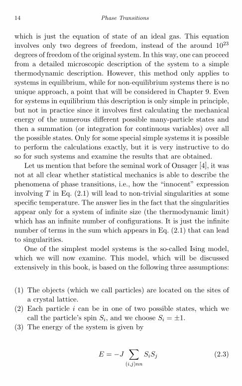
(3) The energy of the system is given by
E = −J∑
(i,j)nn
SiSj (2.3)

June 25, 2004 14:17 WSPC/Book Trim Size for 9in x 6in chap02
The Ising Model 15
where J is a constant and the sum is over all pairs of adjacentparticles, i.e., over all pairs of nearest neighbors i and j. Thus ina linear lattice each particle interacts only with its two nearestneighbors, in a square lattice with its four nearest neighbors, andin a simple cubic lattice with its six nearest neighbors.
In spite of its simplicity, the Ising model is used in many appli-cations where an object can be in one or two states, such as sitesoccupied by A or B atoms, sites containing a particle or a hole,two possible conformations, and even votes for one of two politicalparties in elections. One can generalize the first two basic assump-tions of the Ising model. A larger number of possible states is takeninto account in the so-called Potts model [5], and one can considernot only interactions between nearest neighbors but also interactionsbetween second nearest neighbors, third nearest neighbors, etc. Thesegeneralizations make the problem much more complicated. On theother hand, the lattice approximation seems to be of no importancefor phase transition problems since, as we will see later, much longerdistances (of order of the correlation length) are important in phasetransitions.
The personal story of Ising is also of interest [6]. In 1924–1926,Ising was a doctoral student of the famous German physicist WilhelmLenz, who suggested to him this model. In his thesis, Ising showedthat the system does not exhibit a phase transition in one dimension,which is correct. He also showed that there is no phase transition intwo dimensions, which was shown much later (by Onsager in 1944)to be incorrect. After completing his thesis he started to work as ahigh-school teacher, and with the rise to power of the Nazis he wentto Luxembourg. We next hear of him in 1948 in the USA, where hetaught at some small university. He died in 1990, and during his wholecareer published only two scientific papers, one on his thesis work andthe other entitled “Goethe as a physicist”. However, on his arrivalin America in 1948 he found big placards announcing a conferenceon the Ising model, and this model is still being extensively studiedas a paradigm of a simple system exhibiting a well-defined phasetransition.

June 25, 2004 14:17 WSPC/Book Trim Size for 9in x 6in chap02
16 Phase Transitions
2.1 1D Ising model
We consider first the one-dimensional (1D) Ising model, and exam-ine how to calculate the partition function. Let us assume that thesystem contains N particles, for which the partition function has thefollowing form
ZN =∑
Sj=±1
exp[− J
kT(S1S2 + S2S3 + · · · + SN−1SN )
]. (2.4)
For a system with N + 1 particles, the sum contains one additionalterm, so that
ZN+1 = ZN
∑SN ,SN+1=±1
exp(
− J
kTSNSN+1
). (2.5)
Since SNSN+1 = ±1, it follows that ZN+1 = 2 cosh(J/kT )ZN , andso (since Z1 = 2), by induction,
ZN = 2N
(cosh
J
kT
)N−1
. (2.6)
Hence if N 1 the free energy is
G = −kT lnZ = −NkT ln(
2 coshJ
kT
). (2.7)
Since this is a monotonic function of T , with no singularity exceptat T = 0, the 1D Ising system cannot exhibit a phase transition atany finite temperature.
Another interesting general type of system is the one in whichthe interactions between the particles are very weak but of infiniterange,
ϕ(r) = − limγ→0
γ exp(−γr),
in contrast to the strong short-range interactions of the Ising model.For this model there is a phase transition even in one dimension,and we will discuss it in Chapter 7. In fact, it is not necessary thatthere should be interactions between all the spins in a system for aphase transition to occur. Even a few random long-range interactions

June 25, 2004 14:17 WSPC/Book Trim Size for 9in x 6in chap02
The Ising Model 17
combined with short-range interactions as in the Ising model aresufficient to produce a phase transition, as in the small world modelwhich we discuss in Chapter 8.
2.2 2D Ising model
The exact solution of the 2D Ising model was presented by Onsagerin 1944 in a very long and complicated paper [4], and even after a fewsimplifications, a recent version of the proof took seven pages in thevery concisely written classic text of Landau and Lifshitz [1]. How-ever, we will now present some qualitative arguments for analyzingthe phase transitions in the 2D Ising model.
Since we want to analyze the role of the energy E and the entropyS in order-disorder phase transitions, it is convenient to consider theHelmholz free energy F = E − TS. At all temperatures the sta-ble state corresponds to the minimum value of F . At low tempera-tures the energy E plays the leading role, and its minima correspondto ordered states. At high temperatures the entropy S dominatesF , and so the minima of F are reached when the entropy S is amaximum. Therefore, at some intermediate temperature T = Tc
the ordering influence of the energy and disordering influence ofthe entropy are balanced, and one can qualitatively estimate thecritical temperature Tc as
Tc ≈ ∆E
∆S. (2.8)
In order to apply this equation to the 2D Ising model, we considerthe two competing states of the Ising lattice shown in Fig. 2.1 [7].The question arises as to whether the fully ordered state 1 is ableto transform spontaneously into state 2, which contains an island ofopposite spins with perimeter of length L. For this to happen, thefree energy of state 2 must be lower than that of state 1. To exam-ine when this occurs, let us consider the changes in energy and inentropy when such an island of opposite spins is formed. Since ateach site on the perimeter of the island the energy is raised by 2J ,the energy required to form the island is ∆E = (2J)L. On the other

June 25, 2004 14:17 WSPC/Book Trim Size for 9in x 6in chap02
18 Phase Transitions
Fig. 2.1 2D Ising square lattice, with an island of opposite spins (indicated byblack solid dots) of perimeter L. (B. Liu and M. Gitterman, Am. J. Phys. 71 806(2003). Copyright 2003 by the American Physical Society.)
hand, the number W of microscopic possibilities for creating such anisland is approximately 3L, since from each site one can continue theperimeter in three different directions, and so the change in entropy∆S ≈ ln(3LN), where the factor N arises from an approximate eval-uation of the number of ways in which the initial point can be chosen.This estimate is also approximate because we neglect the necessityto come back to the initial site after L steps, and also the require-ment that the perimeter cannot cross itself. In this approximation,the change in the free energy of the system is
∆F = ∆E − T∆S = L[2J − kT ln 3] − kT lnN (2.9)
and for L of order N the term ln N in this equation can beneglected. Therefore, a disordered state is favored if T > Tc, wherekTc = 2J/ ln 3. This is not a bad approximation to the exact resultfound by Onsager [4],
kTc = 2J/ ln(1 +√
2),
June 25, 2004 14:17 WSPC/Book Trim Size for 9in x 6in chap02
The Ising Model 19
and our analysis shows clearly how the phase transition arises as aresult of the competition between energy and entropy. Incidentally,for the 1D case instead of an island of perimeter L one has a changein the direction of the spin at just one point, so that ∆E = 2J . Onthe other hand, since this point can be anywhere, W = N , so that
∆F = ∆E − T∆S = 2J − kT lnN,
which only becomes negative when kTc = 2J/ lnN , so that Tc → 0as N → ∞. This is in agreement with our previous conclusion thatfor an infinite 1D system, a phase transition can only occur at T = 0.
There is an important general conclusion from our above analy-sis of the 2D Ising model. Both our calculations and the exact oneof Onsager show that kTc is close to J , which is the only energyparameter appearing in our problem. Thus, there is no small param-eter, which is not a happy situation for a physicist, since the theoryof many-body problems usually relies on expressing properties as apower series in a small parameter, such as the ratio of the aver-age potential energy to the average kinetic energy per particle fora weakly non-ideal gas, and the opposite ratio for solids. This isexactly the reason for the absence of a general rigorous theory ofliquids, where these two average energies are of the same order ofmagnitude. It is also one reason why it took so many years to makeprogress in solving the problem of phase transitions.
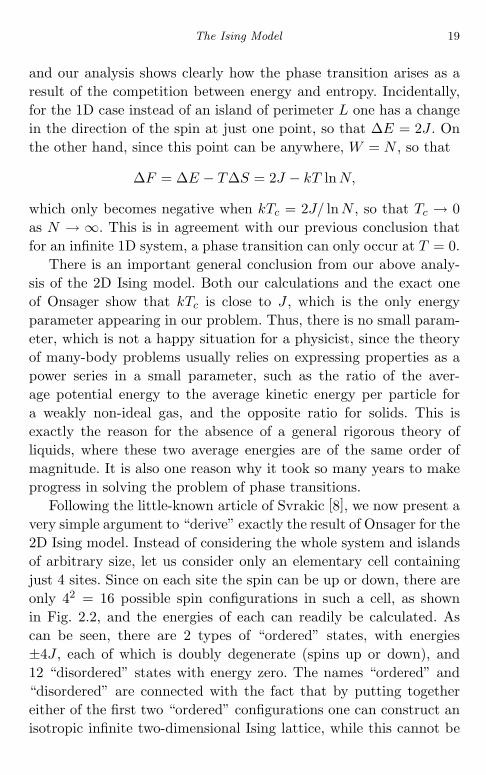
Following the little-known article of Svrakic [8], we now present avery simple argument to “derive” exactly the result of Onsager for the2D Ising model. Instead of considering the whole system and islandsof arbitrary size, let us consider only an elementary cell containingjust 4 sites. Since on each site the spin can be up or down, there areonly 42 = 16 possible spin configurations in such a cell, as shownin Fig. 2.2, and the energies of each can readily be calculated. Ascan be seen, there are 2 types of “ordered” states, with energies±4J , each of which is doubly degenerate (spins up or down), and12 “disordered” states with energy zero. The names “ordered” and“disordered” are connected with the fact that by putting togethereither of the first two “ordered” configurations one can construct anisotropic infinite two-dimensional Ising lattice, while this cannot be

June 25, 2004 14:17 WSPC/Book Trim Size for 9in x 6in chap02
20 Phase Transitions
configurations
Fig. 2.2 Different configurations of an elementary cell of a 2D Ising square latticedivided into four groups, when the energy E and number of configurations N areshown for each group. Groups a and b contain non-degenerate configurations whiledegeneracies are inherent in groups c and d. (B. Liu and M. Gitterman, Am. J.Phys. 71 806 (2003). Copyright 2003 by the American Physical Society.)
done for the “disordered” configurations. In accordance with the ideaof competition between ordered and disordered states, we conjecturethat the phase transition occurs when the partition function of theordered states,
2 exp(
4J
kT
)+ 2 exp
(−4J
kT
),
equals that of the disordered ones, 12, i.e., when x2 +x−2 = 6, wherex = exp(2J/kT ). The solution of this equation is x = 1+
√2, so that
kTc = 2J/ ln(1 +√
2), which quite surprisingly gives the exact resultof Onsager. However, this method as presented above does not workfor a three-dimensional Ising lattice.
2.3 3D Ising model
It is interesting to apply the method described above to the Isingmodel for three-dimensional lattices, and to find the critical temper-ature of these lattices by considering just one elementary cell [9].All the possible 28 = 256 configurations of an elementary cell for asimple cubic lattice are shown in Fig. 2.3, where, as in Fig. 2.2 forthe 2D lattice, N represents the number of equivalent configurations

June 25, 2004 14:17 WSPC/Book Trim Size for 9in x 6in chap02
The Ising Model 21
associated with the appropriate group. Let us consider first the dif-ferent configurations of the 2D Ising lattice shown in Fig. 2.2. We callthe configurations of groups a and b “non-degenerate” in the sensethat all neighboring states, i.e., those that can be obtained from a
Fig. 2.3 Different configurations of the elementary cell of a 3D Ising cubic latticewith N the number of equivalent configurations in each group, and E their energy.Groups a–f contain non-degenerate (stable) configurations, while the configura-tions in groups g and h are degenerate (unstable). Groups i–n make a contribu-tion to the partition function of both degenerate and non-degenerate states, whichare characterized by the fractional statistical weights WG and WN respectively.(B. Liu and M. Gitterman, Am. J. Phys. 71 806 (2003). Copyright 2003 by theAmerican Physical Society.)

June 25, 2004 14:17 WSPC/Book Trim Size for 9in x 6in chap02
22 Phase Transitions
given one by the flipping of a single spin, have an energy differentfrom that of the original one. By contrast, all the configurations con-tained in group c do not change their energy if one of the spins isflipped. Hence, these configurations have adjacent states of the sameenergy, and with respect to this property we call these configurations“degenerate”. The situation is slightly more complicated for the con-figurations belonging to group d. Here, flipping spin 1 will change theenergy by 4J , while flipping spin 4 will lead to a change in energyof −4J . Due to the symmetry of the latter two states with respectto the original one with E = 0, we place this “quasi-degenerate”state in the “degenerate” group. We note that flipping spins 2 or 3will not change the energy. Hence, all configurations of group d arerelated, along with those of group c, to “degenerate” configurations.Our conjecture consists of the statement that the phase transitionoccurs when the partition function Zndg of non-degenerate states isequal to that Zdg of degenerate states,
Zndg = Zdg, (2.10)
i.e., we identify the non-degenerate states with “ordered” configura-tions and the degenerate states with “disordered” ones.
Since for the two-dimensional Ising lattice our criterion (2.10)coincides with that of Svrakic [8], it clearly results in the exactOnsager solution for the critical temperature. However, in contrast to[8], our criterion (2.10) can be applied to three-dimensional latticesas well. We now examine Fig. 2.3 in detail. Here, groups a–f belongto the non-degenerate category, because a flip of the spin of any sitewill change the energy of the cell, and no quasi-degenerate states areobserved in these configurations. Groups g and h belong to the degen-erate category. A flip of each spin of group g results in the change ofenergy of 2J,−2J, 2J,−2J, 2J,−2J, 2J,−2J , while a flip of each spinof group h change the energy by 6J,−6J, 6J,−6J, 2J,−2J, 2J,−2J ,and these two groups are totally quasi-degenerate. However, groupsi–n contribute to both degenerate and non-degenerate states. Let usconsider, as an example, group i. The flip of each of the eight spinschanges the energy by −6J, 6J, 6J, 6J, 6J, 2J, 2J, 2J , respectively. The

June 25, 2004 14:17 WSPC/Book Trim Size for 9in x 6in chap02
The Ising Model 23
first two excited states are symmetric, and, according to our classifi-cation, they are quasi-degenerate, while the remaining six states arenon-degenerate. The numbers shown in Fig. 2.3 are the statisticalweight of degenerate WG and non-degenerate WN states, and so forgroup i they have the fractional values 2/8 and 6/8 respectively. Anal-ogous analyses can easily be performed for each of the groups j–n,and the final result for the solution of Eq. (2.10) is kTc/J = 4.277 [9]which is much closer to the numerical result kTc/J = 4.511 [10] thanthat, kTc/J = 2.030, obtained by the method of Ref. [8].
In conclusion, we have shown that the critical temperature oftwo- and three-dimensional Ising models can be obtained by sim-ple physical arguments based on the compromise between configura-tions which are “degenerate” or “non-degenerate” with respect to asingle spin-flip excitation. A challenging problem for the interestedreader is to expand our calculations to other elementary cells of two-dimensional lattices (say, 3–3 square, 3–2 rectangle, etc.) and to othertypes of three-dimensional lattices (BCC, FCC, etc.). For the latter,the findings have to be compared with the precise numerical resultswhich are 6.235 and 9.792 for the BCC and FCC lattices, respectively[10]. The results of such a comparison are not known a priori sinceit is not clear how well this method will work in the general case.
2.4 Conclusion
The microscopical analysis of phase transitions can be performedonly for simple models such as the Ising model. The results forthese show that for non-zero temperature a phase transition doesnot appear in a one-dimensional system but such a transition doesoccur in two dimensions. A qualitative explanation of the onset of aphase transition as an order–disorder transition is that it is a result ofcompetition between the ordering tendency of the energy and the dis-ordering tendency of the entropy. With some simplified conjectures,such considerations can even lead to quantitatively correct results.

This page intentionally left blank

June 25, 2004 14:17 WSPC/Book Trim Size for 9in x 6in chap03
Chapter 3
Mean Field Theory
As we mentioned in Chapter 1, the simplest way to allow for inter-actions between particles is the mean field approximation, in whichone assumes that the environment of each particle corresponds tothe average state of the system and determines this average stateself-consistently.
In order to understand the nature of Weiss’ mean field approxi-mation described in Chapter 1, it is useful to examine the applicationof this approximation to the Ising model. In this model, the energyof a state of the system with a given arrangement S1, S2, . . . , SNof the N spins Sj , each of which can have the value ±1, situated ona lattice of sites, is
E = −J∑
(i,j)nn
SiSj . (3.1)
In Weiss’ mean field approximation for our system,
Emf = −∑
i
SiHm (3.2)
where Hm is the effective magnetic field. A comparison of Eqs. (3.1)and (3.2) shows that Hm = J〈Sj〉, so that
Emf = −J∑
(i,j)nn
Si〈Sj〉. (3.3)
25

June 25, 2004 14:17 WSPC/Book Trim Size for 9in x 6in chap03
26 Phase Transitions
Now, Eq. (3.1) can be written in the form
E = −J∑
(i,j)nn
Si〈Sj〉 − J∑
(i,j)nn
Si(Sj − 〈Sj〉)]. (3.4)
The first term in this equation is the expression that we derived forthe mean field approximation, while the second term arises from thefluctuations of each spin from its mean value. Hence the mean fieldapproximation is equivalent to ignoring fluctuations. It is obviousthat as the number of dimensions of the system increases, and withit the number of nearest neighbors of each site, the importance ofthese fluctuations decreases, and they are negligible for a systemof sufficiently high dimensions. As we will see later on, “sufficientlyhigh” for the Ising systems means d > 4. This is the physical reasonwhy for each system there is an upper critical dimension above whichthe mean field approximation is valid.
3.1 Landau Mean Field Theory
We now consider the thermodynamic approach to mean field theoryproposed by Landau. He suggested [1] introducing an extra param-eter η, which is called an order parameter, to distinguish the phaseof the system, so that the Gibbs free energy G is now a function ofthree parameters, G = G(P, T, η), where η = 0 in a disordered statefound, as a rule, at high temperatures, T > Tc, and η = 0 for theordered state, which then occurs for T < Tc. Since the free energy ofthe system in equilibrium is uniquely determined by P and T , thisorder parameter must be a function of them, η = η(P, T ). The firstassumption of Landau’s mean field theory is that an order parame-ter can be defined such that ∂G/∂η = 0 and ∂2G/∂η2 > 0, whichis the natural condition for minima of the free energy. His secondassumption is based on the fact that at the phase transition η = 0.Therefore, close to the phase transition point he assumed that G canbe expanded as a power series in η,
G(P, T, η) = G0(P, T ) + αη + Aη2 + βη3 + Bη4 + · · · (3.5)
June 25, 2004 14:17 WSPC/Book Trim Size for 9in x 6in chap03
Mean Field Theory 27
where all the coefficients are functions of P and T . The first assump-tion, ∂G/∂η = 0, can only be satisfied for all η if α = 0. For amagnetic system in which the magnetic moment vector is the orderparameter, symmetry arguments show that it is not possible to forma scalar from η3, and so β = 0. Incidentally, for different systemsthe order parameter can have different numbers of components. Forinstance, in the liquid–gas phase transition the order parameter is thedifference in densities between the two phases, which is a scalar. Insuperfluidity and superconductivity, it is the wave function ψ whichhas two components (its real and imaginary parts, or its amplitudeand phase). For the anisotropic Heisenberg ferromagnet, in which M
has three independent components, this will also be true of η.Here we restrict our attention to systems in which η has just one
component, and for which close to the phase transition point the freeenergy can be written in the form
G(P, T, η) = G0(P, T ) + Aη2 + Bη4. (3.6)
For the sake of simplicity, we consider systems at a constant pressureequal to the critical one, P = Pc, and so omit P from the arguments.Then for arbitrary η the requirement that ∂G/∂η = 0 means that2Aη +4Bη3 = 0, so that η = 0 for T > Tc, and there is an additionalsolution η2 = −A/(2B) for T < Tc. From the second requirement∂2G/∂η2 > 0 it follows that for T > Tc, A > 0 while A < 0 forT < Tc. It follows that A(Tc) = 0, and the simplest form for A thatsatisfies these conditions is A = a(T − Tc), with a > 0. One thenfinds that the order parameter
η ∼√
Tc − T (3.7)
and the free energy
G(T, η) = G0(T ) + a(T − Tc)η2 + Bη4. (3.8)
Here the term in η4 is required since the term in η2 vanishes at thecritical point, but the temperature dependence of its coefficient B
can be ignored, so that we can write B = B(Tc, Pc).
June 25, 2004 14:17 WSPC/Book Trim Size for 9in x 6in chap03
28 Phase Transitions
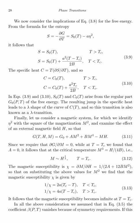
We now consider the implications of Eq. (3.8) for the free energy.From the formula for the entropy
S = −∂G
∂T= S0(T ) − aη2,
it follows that
S = S0(T ), T > Tc,
S = S0(T ) +a2(T − Tc)
2B, T < Tc.
(3.9)
The specific heat C = T (∂S/∂T ), and so
C = C0(T ), T > Tc,
C = C0(T ) +a2Tc
2B, T < Tc.
(3.10)
In Eqs. (3.9) and (3.10), S0(T ) and C0(T ) arise from the regular partG0(P, T ) of the free energy. The resulting jump in the specific heatleads to a λ shape of the curve of C(T ), and so this transition is alsoknown as a λ-transition.
Finally, let us consider a magnetic system, for which we identifyη2 with the square of the magnetization M2, and examine the effectof an external magnetic field H, so that
G(T, H, M) = G0 + AM2 + BM4 − MH. (3.11)
Since we require that ∂G/∂M = 0, while at T = Tc we found thatA = 0, it follows that at the critical temperature M3 = H/(4B), i.e.,
M ∼ H13 , T = Tc. (3.12)
The magnetic susceptibility is χ = ∂M/∂H = 1/(2A + 12BM2),so that on substituting the above values for M2 we find that themagnetic susceptibility χ is given by
1/χ = 2a(Tc − T ), T < Tc,
1/χ = 4a(T − Tc), T > Tc.(3.13)
It follows that the magnetic susceptibility becomes infinite at T = Tc.In all the above consideration we assumed that in Eq. (3.5) the
coefficient β(P, T ) vanishes because of symmetry requirements. If this
June 25, 2004 14:17 WSPC/Book Trim Size for 9in x 6in chap03
Mean Field Theory 29
is not the case, all the above calculations are correct provided that inaddition β(Pc, Tc) = 0 at the critical point, as well as A(Pc, Tc) = 0.However, these two conditions mean that the critical point is anisolated point in the T–P plane — a case which is of no specialinterest.
We note that all the results obtained in Eqs. (3.7)–(3.13) forthe temperature dependence of the thermodynamic parameters donot involve the spatial dimensions. This is not correct, as we willsee later on. Such a failing should not surprise us, since the meanfield approach is based, in particular, on the assumption of analyt-icity, which is at least questionable for a function which may havesingularities.
3.2 First Order Phase Transitions in Landau Theory
So far, we have considered only continuous (second order) phasetransitions. However, the Landau mean field theory is also able todescribe first order phase transitions, where there is a jump in theorder parameter. There are two different ways of doing this:
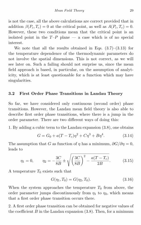
1. By adding a cubic term to the Landau expansion (3.8), one obtains
G = G0 + a(T − Tc)η2 + Cη3 + Bη4. (3.14)
The assumption that G as function of η has a minimum, ∂G/∂η = 0,leads to
η1 = 0, η2 = −3C
8B±
√(3C
8B
)2
− a(T − Tc)2B
. (3.15)
A temperature T0 exists such that
G(η1, T0) = G(η2, T0). (3.16)
When the system approaches the temperature T0 from above, theorder parameter jumps discontinuously from η1 to η2, which meansthat a first order phase transition occurs there.
2. A first order phase transition can be obtained for negative values ofthe coefficient B in the Landau expansion (3.8). Then, for a minimum

June 25, 2004 14:17 WSPC/Book Trim Size for 9in x 6in chap03
30 Phase Transitions
of G (M) to exist, one has to consider the sixth order term in theexpansion of G(M),
G = G0 + a(T − Tc)M2 − |B|M4 + DM6. (3.17)
The conditions for a minimum of Eq. (3.17) lead to
M1 = 0, M2 =1√3D
[|B| +√
B2 − 3aD(T − Tc)] 1
2 . (3.18)
By using a procedure identical to that used for the analysis ofEq. (3.16), we conclude that a first order phase transition occursin this case as well.
3.3 Landau Theory Supplemented with Fluctuations
As we showed earlier in this chapter, the difference between theresults of mean field theory and the exact results are due to fluctua-tions. We now generalize the Landau theory by taking into accountthese fluctuations. In order to do this, the first step is to use thequasi-hydrodynamical approach, and replace the discrete lattice bya continuum, so that the free energy G and the order parameter, M
in the case of ferromagnetism, become functions of the continuouscoordinate r, G = G(r) and M = M(r). Then the global expansion(3.8) has to be replaced by a local one for G(r), while the global freeenergy and magnetic moment are obtained by integration over thewhole d-dimensional system.
For a non-homogeneous system the expansions of the free energywill contain not only the thermodynamic variables but also theirderivatives. Assuming that the inhomogeneities are small, one canretain in the expansions only the simple gradient term (∇M)2, andneglect higher derivatives. There is no need to multiply this termby a constant since the length scale can be chosen to make thisconstant unity. Thus, the simplest possible form for the free energydensity G(r) is
G(r) = G0 + AM2 + BM4 + (∇M)2. (3.19)

June 25, 2004 14:17 WSPC/Book Trim Size for 9in x 6in chap03
Mean Field Theory 31
According to Boltzmann’s formula, the probability for a fluctuationP (M) is proportional to exp[−(G − G0)/kT ], and so
P (M) ∼ exp[−
∫dτ
AM2 + (∇M)2
kT
]. (3.20)
Here, we ignore the term BM4 since this was only introduced toprevent G − G0 vanishing at the critical point, where A = 0, whilethe extra term (∇M)2 ensures that this does not happen. Thus, weuse a Gaussian approximation, i.e., one that involves only quadraticterms in M and ∇M .
In order to calculate the above integral, it is convenient to use theFourier transform of M(r),
M(r) =∫
MK exp(iK · r) ddK. (3.21)
The radial distribution function g(r) of M(r) is determined by thecoefficients MK [1],
g(r) =∫
M(R)M(R + r) dR∫M(R)M(R) dR
=∫
〈M2K〉 exp(iK · r) ddK. (3.22)
According to the Gaussian approximation (3.20), the probability ofa fluctuation described by a given set MK of Fourier coefficients is
PMK ∼ exp[−(A + K2)M2
KkT
]≡ exp
(− M2
K
2〈M2K〉
), (3.23)
where 〈M2K〉 = kT/[2(A + K2)]. On substituting this expression in
Eq. (3.22), we find that
g(r) =∫
kT exp(iK · r)2(A + K2)
ddK. (3.24)
It follows, e.g. from integration in the complex plane and the residuetheorem, that in three dimensions
g(r) ∼ exp(−r√
A)r
(3.25)

June 25, 2004 14:17 WSPC/Book Trim Size for 9in x 6in chap03
32 Phase Transitions
so that the correlation length
ξ =1√A
∼ (T − Tc)−1/2. (3.26)
At the critical point A = 0, and so at T = Tc the correlation functionbecomes
g(r) ∼ 1r. (3.27)
3.4 Critical Indices
In the theory of phase transitions, it is very important to describethe behavior of various properties of the system in the vicinity of thecritical point. For a differentiable function with a singularity at thecritical point, such as a ∼ |T − Tc|x, this behavior is characterizedby the index x, which is called a critical index. If x = 0, this criticalindex is given by x = ln(a)/ ln |T − Tc|, while if x = 0 there are twopossibilities. In one case, a becomes a constant at the critical point,with the possibility of different values of this constant on the twosides of the transition, which is a jump singularity. In the other case, a
exhibits a logarithmic singularity, a ∼ ln |T −Tc|. For other propertiesof the system near and at the critical point, the power exponents ofthese dependencies are called critical indices. In Table 4.1 in the nextchapter, we define a set of critical indices and present their valuesfor the mean field model calculated above, as well as the values ofthe critical indices for some other models which we analyze there.
3.5 Ginzburg Criterion
Since the difference between the results of mean field theory andthe exact ones is due to the fluctuations in the order parameter,we expect that the mean field approximation will be accurate whenthese fluctuations are sufficiently small. Ginzburg proposed [11] thatthe mean field theory is applicable when the fluctuations are small incomparison with the thermodynamical values. On using Eq. (3.23)and the fact that M2 ∼ A, one finds after integrating over angles

June 25, 2004 14:17 WSPC/Book Trim Size for 9in x 6in chap03
Mean Field Theory 33
that this criterion is fulfilled if∫ Kmax
0kT
Kd−1
A + K2 dK < |A|. (3.28)
If the dependence of the integral on its upper limit can be neglected,it follows from the substitution y = K
√A that this condition
becomes
(Ad/2/A)∫
f(y)dy A,
and so Ad/2 A2. Hence, since A is small in the region of the criticalpoint, the mean field approximation is valid if d > 4, so that theupper critical dimension is four. For d = 4 there are only logarithmiccorrections to the mean field results.
While the above estimates are simple but crude, they still provideus with useful information. If one takes into account the coefficientsin the inequality (3.28), and substitutes their values for differenttypes of phase transitions, qualitative estimates can be obtained ofthe region around the critical point where the mean field theory isvalid. It turns out that for the gas–liquid phase transition the meanfield theory can be applied up to within ten percent of the criticaltemperature, while for the superconducting transitions the mean fieldtheory gives the correct results everywhere in the experimentallyaccessible vicinity of the critical point. The latter result is connectedwith the large value of the correlation length in low temperaturesuperconductors.
3.6 Wilson’s ε-Expansion
So far, we have considered the local value η(r) associated with thepoints r of a lattice, which are a distance a apart and can be regardedas a continuum, so that in our previous analysis we often used inte-grals rather than sums. Such a coarse-graining procedure does notlead to any problems in hydrodynamics, where a is the only charac-teristic length, as soon as the condition r > a is satisfied. However,as Wilson pointed out [12], this coarse-graining procedure becomes

June 25, 2004 14:17 WSPC/Book Trim Size for 9in x 6in chap03
34 Phase Transitions
problematic in the theory of phase transitions, since near the criticalpoint the correlation length ξ appears as an additional character-istic length. Hence, the simple coarse-graining procedure for r > a
becomes unjustified unless in addition r > ξ, and one has to findsome way to treat the range a < r < ξ. This region is very importantnear the critical point, since ξ tends to infinity as the critical pointis approached.
In order to deal with this problem, Wilson suggested that, incontrast to the situation for hydrodynamics, the coefficients A and B
in Eq. (3.19) depend on the size of the coarse-graining region, whichwe denote by L. In order to find these dependencies let us considerhow the free energy changes when one goes from a region of size L,with a < L < ξ, to a region of size L+∆L. Such a comparison of thefree energies in two regions is, in fact, the basis of the renormalizationgroup approach which we will consider in detail in Chapter 5.
Let us consider a value of ∆L so small that it introduces justone additional mode into a system. If we label the modes by theirFourier components K, this means [1] that V 4πKd−1∆K/(2π)3 = 1,or since K ∼ 1/L that, for V = 1, ∆L ∼ Ld+1. Let us now write thefree energy GL+∆L(P, T ) in the Landau form (3.19),
GL+∆L(M) =∫
dτ [G0+AL+∆LM2+BL+∆LM4+(∇M)2] (3.29)
and compare it with that obtained from GL(P, T ) supplemented byan additional fluctuating mode mM1 with a scaling factor m:
GL(M + mM1) =∫
dτ[G0 + AL(M + mM1)2
+ BL(M + mM1)4 + [∇(M + mM1)]2]. (3.30)
The contribution of the additional mode mM1 will be taken intoaccount not by the “hydrodynamic” average but by the correct“Boltzmann” average. Thus, one finds that
exp(
−GL+∆L
kT
)=
∫ ∞
−∞dm exp
(−GL(M + mM1)
kT
). (3.31)

June 25, 2004 14:17 WSPC/Book Trim Size for 9in x 6in chap03
Mean Field Theory 35
We restrict our attention to the Gaussian distribution, and so leave inthe exponent of the right hand side of Eq. (3.31) only terms quadraticin m, and require that for the fluctuating mode∫
M1(r)dr = 0,
∫M2
1 (r)dr = 1. (3.32)
For small ∆L one can write
AL+∆L = AL +dA
dL∆L, BL+∆L = BL +
dB
dL∆L. (3.33)
The substitution of Eqs. (3.32) and (3.33) into Eq. (3.31) leads tothe equation
dAL
dL∆LM2 +
dBL
dL∆LM4
= Const + ln(1 + ALL2 + 6BLL2M2). (3.34)
On expanding the logarithm in (3.34) in a power series and equatingthe coefficients of M2 and M4, we find that
dA
dL∆L = 3BL2 − 3ABL4,
dB
dL∆L = −9B2L4.
(3.35)
Since ∆L ∼ Ld+1, this gives in terms of the parameter ε ≡ 4 − d,
A ∼ L− ε3 , B ∼ L−ε. (3.36)
Equations (3.36) must be valid for a < L < ξ, and so we substitute inthem L = ξ. On using Eq. (3.26) for ξ and A = a(T − Tc), one findsfrom Eq. (3.36) that M ∼ [(T − Tc)/Tc]β and ξ ∼ (|T − Tc|/Tc)−ν
where
β =12
− ε
6(1 − ε
6
) , ν =1
2(1 − ε
6
) . (3.37)
This equation gives the values of the critical indices, which weredefined in the last section and are listed in Table 4.1. In this equation,the critical indices are expanded as power series in the small param-eter ε, which is why the method is known as Wilson’s ε-expansion.Not by chance is Wilson’s article [13] called “Critical phenomena in3.99 dimensions”. If one is brave enough to set the “small” parameter
June 25, 2004 14:17 WSPC/Book Trim Size for 9in x 6in chap03
36 Phase Transitions
ε equal to unity, ε = 1, then the one finds that for three-dimensionalsystems the critical indices are β = 0.3 and ν = 0.6.
The above approximate calculation, which gives the ε-correctionsto the mean field critical indices, is a good introduction to the renor-malization group approach, where this transformation leading fromGL to GL+∆L is applied repeatedly.
3.7 Conclusion
The simplest phenomenological mean field description of phase tran-sitions is obtained by introducing an order parameter η and assumingthat close to the critical point the free energy G can be expandedin this order parameter. The requirement that G(η) be a minimumenables us to find the critical indices which define the behavior ofthe thermodynamical parameters near the critical point. As it followsfrom comparison of Weiss’ mean free theory with the Ising model, themain approximation of the mean field theory is the neglect of fluctu-ations. According to the Ginzburg criterion, this is justified for spacedimensions larger than four (the upper critical dimension). The inclu-sion of fluctuations in the mean field theory is achieved by adding tothe free energy the simplest gradient terms, and this enables us tofind the temperature dependence of the correlation length and theform of the correlation function at the critical point.
Another type of correction to the mean field theory is associatedwith the increase of the correlation length on approaching the crit-ical point. These corrections are taking into account by introducingthe spatial dependence of the coefficients in an expansion G = G(η).This leads to the dependence of the critical indices on the parameterε = 4 − d, which defines the distance from the upper critical dimen-sion d = 4. This ε-expansion is the simplest form of a renormalizationgroup procedure.

June 25, 2004 14:17 WSPC/Book Trim Size for 9in x 6in chap04
Chapter 4
Scaling
Scaling is a very general and well-known method for describing theresponse of a system to a disturbance. For physical systems, it is mostreadily studied in terms of dimensional analysis and the constructionof dimensionless parameters, and so we consider this topic first, andstart with a few simple examples.
Let us consider first the free fall (i.e., with no air resistance) ofa body of mass m under the gravitational force mg. If the bodystarts from rest, then we expect that its velocity v after falling froma height h will be a function of m, h, and g, v = f(m, h, g). Weassume that v has a power-law dependence on these parameters, andso write v = amαhβgγ , where a is a dimensionless constant. In anyequation, the dimensions of the quantities on the two sides must beequal. Since [v] = LT−1, [h] = L, [m] = M and [mg] = MLT−2, itfollows that
LT−1 = MαLβ(LT−2)γ (4.1)
which has the unique solution α = 0, β = γ = 1/2, so that v = a√
gh.Thus, we have found the functional dependence of v on g and h
without having to solve the problem, and can conclude that if theheight from which the body falls is multiplied by four then its velocitywill be doubled.
Another example, which is very relevant for engineering applica-tions, is the force F acting on a sphere of radius R moving througha fluid of viscosity η with velocity v. We assume that F = aRαvβηγ ,
37
June 25, 2004 14:17 WSPC/Book Trim Size for 9in x 6in chap04
38 Phase Transitions
and once again equate the dimensions of the two sides of this equa-tion. Since [F ] = MLT−2, [R] = L, [v] = LT−1, and [η] = ML−1T−1,it follows that α = β = γ = 1, so that F = aRvη, which is justStokes’ law. This law permits the prediction of such properties asthe air resistance to the motion of cars or aeroplanes from those ofmodel systems with smaller objects and/or lower velocities, althoughallowance has to be made for the fact that cars and aeroplanes arenot spherical. An important point about this example, in contrast tothe first one, is that we had to decide (or guess) which of the fourparameters in the system, namely the radius, velocity and mass ofthe object and the viscosity of the medium, was irrelevant, since formechanical (as opposed to electromagnetic) quantities there are onlythree independent dimensions, namely mass M, length L and time T.
Scaling is also of considerable importance for presenting theo-retical predictions and experimental data for different values of theparameters on a single curve. The basis for such a procedure is thata homogeneous function f(x, y) of x and y of order p is defined bythe requirement that
f(λx, λy) = λpf(x, y). (4.2)
Then, on choosing λ = 1/x, one finds that f(1, y/x) = (1/x)pf(x, y),so that
f(x, y) = xpf(1,
y
x
)= xpψ
(y
x
). (4.3)
Equation (4.3) means that a homogeneous function of two variablescan be scaled to a function of a single variable, so that by a suitablechoice of variables (f(x, y)/xp and y/x) all of the data collapse on toa single curve.
One can also consider [14] a generalized homogeneous function
f(λax, λby) = λpf(x, y) (4.4)
which for a = b reduces to a standard homogeneous function (4.2).

June 25, 2004 14:17 WSPC/Book Trim Size for 9in x 6in chap04
Scaling 39
4.1 Relations Between ThermodynamicCritical Indices
Critical indices, which were introduced in previous chapters, definethe behavior of the thermodynamic parameters near the criticalpoint. A list of such indices, with their definitions, is given inTable 4.1. While the definitions listed there are for a magnetic sys-tem, they can easily be formulated for other types of system. Forinstance, for the liquid–gas system, the magnetic field H is replacedby the pressure P , and the magnetic moment M by the specific vol-ume. The different thermodynamic parameters are not independent,since there are some thermodynamic relations between them, andthese lead to connections between different critical indices. We nowconsider two examples of such relations.
The well-known formula [1] linking specific heats in magnetic sys-tems, cH and cM (or cp and cv for non-magnetic systems) has thefollowing form:
cH − cM =T (∂M/∂T )2H(∂M/∂H)T
. (4.5)
Table 4.1 Critical indices for the specific heat (α), order parameter (β),susceptibility (γ), magnetic field (δ), correlation length (ν) and correlation func-tion (η). The indices α, γ, ν and α′, γ′, ν′ refer to T > Tc and T < Tc, respectively.The results for the mean field and 2D Ising models are exact, while those for the3D Ising model are approximate.
Exponent Definition Condition Mean field 2D Ising 3D Ising
α C ∼∣∣∣T−Tc
Tc
∣∣∣−α(−α′)
H = 0 0 (jump) 0 (ln) ∼0.11
β M ∼(
Tc−TTc
)β
H = 0; T < Tc 0.5 0.125 ∼0.32
γ χ ∼∣∣∣T−Tc
Tc
∣∣∣−γ(−γ′)
H = 0 1 1.75 ∼1.24
δ H ∼ |M |δ T = Tc 3 15 ∼4.82
ν ξ ∼∣∣∣T−Tc
Tc
∣∣∣−ν(−ν′)
H = 0 0.5 1 ∼0.63
η g(r) ∼ 1rd−2+η T = Tc 0 0.25 ∼0.03

June 25, 2004 14:17 WSPC/Book Trim Size for 9in x 6in chap04
40 Phase Transitions
In order for a system to be stable, cM must be positive, and so itfollows from Eq. (4.5) that
cH >T (∂M/∂T )2H(∂M/∂H)T
(4.6)
or, on substituting the critical indices from Table 4.1,
τ−α > τ2(β−1)+γ (4.7)
where τ = |T − Tc|/Tc. Close to the critical point τ 1, and soEq. (4.7) leads [15] to the following relation between the criticalindices
α + β + 2γ ≥ 2. (4.8)
Another inequality can be obtained as follows [16]. For T1 < Tc,
G(Tc, M1) = G(T1, M1)+∫ Tc
T1
(∂G
∂T
)M
dT = G(T1, M1)−∫ Tc
T1
SdT.
(4.9)However, since the stability condition requires that
cM ∼ −(
∂2G
∂T 2
)M
> 0,
the derivative(
∂G∂T
)must be a decreasing function of T , and so
S = − (∂G∂T
)M
must be an increasing function of T . It follows thenfrom Eq. (4.9) that
G(Tc, M1) ≤ G(T1, M1) − (Tc − T1)S(T1, M1), (4.10)
and
G(Tc, M1) ≥ G(T1, M1) − (Tc − T1)S(Tc, M1). (4.11)
For T < Tc, a magnetic moment M(T ) appears spontaneously,so that G(T, M(T )) and S(T, M(T )) are fully determined by thetemperature T , and so Eq. (4.10) can be rewritten in the form
G(T1) ≥ G(Tc) + (Tc − T1)S(T1). (4.12)
On adding Eqs. (4.12) and (4.11), we obtain
G(Tc, M1) − G(Tc) ≤ (Tc − T1)[S(Tc) − S(T1)]. (4.13)
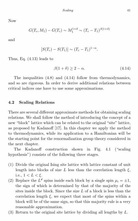
June 25, 2004 14:17 WSPC/Book Trim Size for 9in x 6in chap04
Scaling 41
Now
G(Tc, M1) − G(Tc) ∼ M1+δ1 ∼ (Tc − T1)β(1+δ)
and
[S(Tc) − S(T1)] ∼ (Tc − T1)1−α.
Thus, Eq. (4.13) leads to
β(1 + δ) ≥ 2 − α. (4.14)
The inequalities (4.8) and (4.14) follow from thermodynamics,and so are rigorous. In order to derive additional relations betweencritical indices one have to use some approximations.
4.2 Scaling Relations
There are several different approximate methods for obtaining scalingrelations. We shall follow the method of introducing the concept of anew “block” lattice which can be related to the original “site” lattice,as proposed by Kadanoff [17]. In this chapter we apply the methodto thermodynamics, while its application to a Hamiltonian will bethe starting point for the renormalization group theory considered inthe next chapter.
The Kadanoff construction shown in Fig. 4.1 (“scalinghypothesis”) consists of the following three stages.
(1) Divide the original Ising site lattice with lattice constant of unitlength into blocks of size L less than the correlation length ξ,i.e., 1 < L < ξ.
(2) Replace the Ld spins inside each block by a single spin µi = ±1,the sign of which is determined by that of the majority of thesites inside the block. Since the size L of a block is less than thecorrelation length ξ, we expect that most of the spins within ablock will be of the same sign, so that this majority rule is a veryreasonable approximation.
(3) Return to the original site lattice by dividing all lengths by L.

June 25, 2004 14:17 WSPC/Book Trim Size for 9in x 6in chap04
42 Phase Transitions
Fig. 4.1 The Kadanoff construction for a square lattice, with blocks of nine sites.
The aim of this procedure is to make an average over the smalldegrees of freedom, or in other words to make a coarse graining soas to reduce the number of degrees of freedom of the system. Theconsequences of this idea are not at all trivial. Even if we do notknow the exact solution of the problem for either the site lattice orthe block lattice, a comparison of these two problems can provide uswith valuable information.
Since all the thermodynamic properties of a system depend onlyon the temperature and the external magnetic field, which determineits free energy, let us consider a site lattice in an external (dimen-sionless) magnetic field h and in contact with a thermal bath attemperature T , which appears in our analysis in the dimensionlessform τ = |T −Tc|/Tc. Let the corresponding parameters for the blocklattice be h′ and τ ′. It is obvious that if there is no external field forthe site lattice so that h = 0, then there is no such field for the blocklattice so that h′ = 0, and similarly if τ = 0 then τ ′ = 0. In view ofthis, and since the single parameter that characterizes the size of theblock lattice is L, Kadanoff proposed that τ ′ = Lxτ and h′ = Lyh.
Let f(τ, h) be the free energy per site for the site lattice, andf(τ ′, h′) the free energy per block of the block lattice. Since the freeenergy of a block is the sum of the free energy of the sites composingit, it follows that in d dimensions
Ldf(τ, h) = f(τ ′, h′) = f(Lxτ, Lyh). (4.15)

June 25, 2004 14:17 WSPC/Book Trim Size for 9in x 6in chap04
Scaling 43
As can be seen by substitution, a solution of this functionalequation is
f(τ, h) = τd/xψ(τ/hx/y), (4.16)
where ψ is an arbitrary function. This property enables us to findthe connection between the critical indices associated with differentproperties of the system without knowing the function ψ.
The magnetic moment
M ∼ [∂f/∂h]h=0 ∼ τd/x[τ/h1+x/y]ψ′(z),
where z = τ/hx/y. The only way that this can be independent ofh as h → 0 is that for z −→ ∞, ψ′(z) ∼ z−1−y/x, in which caseM ∼ τ (d−y)/x. Hence, the critical index β defined in Table 4.1, isgiven by
β =d − y
x. (4.17)
It then follows that the magnetic susceptibility as h → 0, i.e.,as z → ∞,
χ ∼ ∂M/∂h ∼ τd/x[τ/h1+x/y]2ψ′′(z),
and thus ψ′′(z) ∼ z−2−2y/x, so that χ ∼ τd/x+2−2−2y/x, and hence
γ =2y − d
x. (4.18)
The specific heat as h → 0, i.e., as z → ∞, C ∼ ∂2f/∂τ2 ∼ τd/x−2,and so
α = 2 − d
x. (4.19)
At the critical point, τ = 0, the temperature-independent magneticmoment M ∼ τd/x[τ/h1+x/y]ψ′(z) requires ψ′(z) ∼ z−(1+d/x) asz → 0. A new critical index δ is defined by M ∼ h1/δ at τ = 0.It then follows that
δ =y
d − y. (4.20)

June 25, 2004 14:17 WSPC/Book Trim Size for 9in x 6in chap04
44 Phase Transitions
In order to obtain more critical indices, let us now consider thecorrelation function g(r, τ) in the site and block lattices. The firststep is to derive the relationship between the average spins 〈S〉 ofthe site lattice and 〈µ〉 of the block lattice. To do this, we comparethe average energy per block of Ld spins in an external magnetic fieldh in the site lattice with the energy per block in the correspondingexternal magnetic field h′ = Lyh in the block lattice
hLd〈S〉 = hLy〈µ〉. (4.21)
It follows that 〈S〉 ∼ Ly−d〈µ〉, or for the correlation functions gs andgµ in the site and block lattices, respectively,
gs(r, τ) = L2(y−d)gµ
( r
L, Lxτ
). (4.22)
It can easily be proved by substitution that the solution of the func-tional equation (4.22) has the following form
gs(r, τ) = r2(y−d)Ψ(rτ1/x) (4.23)
where Ψ is an arbitrary function. At the critical point, τ = 0, thelimiting form of Ψ(z) has to be Ψ(z) ∼ constant and so gs(r, τ) ∼r2(y−d). On comparing this with the definition of the critical indicesin Table 1, one finds that
2y − d = 2 − η. (4.24)
The characteristic length enters Eq. (4.23) in the form rτ1/x, i.e., forthe correlation length ξ one obtains ξ ∼ τ−1/x, or
1x
= ν (4.25)
Thus, the Eqs. (4.17)–(4.20) and (4.24)–(4.25) define six relationsbetween the critical indices. On eliminating from these relations theunknown parameters x and y, one finds the following four relationsbetween different critical indices
α + β + 2γ = 2, βδ = β + γ, γ = ν(2 − η), α = 2 − dν.
(4.26)

June 25, 2004 14:17 WSPC/Book Trim Size for 9in x 6in chap04
Scaling 45
The above analysis makes it clear that when the critical indicesare define for T > Tc and T < Tc, the calculations can be performedin both cases so that the limiting behavior of the thermodynamicfunctions is symmetric with respect to Tc, i.e.
α = α′, ν = ν ′, γ = γ′. (4.27)
Equations (4.26) and (4.27) show that, within the framework of thescaling hypothesis, there are seven relations between the nine ther-modynamic critical indices, i.e., only two indices are independent.These two remaining indices will be found in the next chapter by theuse of the renormalization group theory.
Since the scaling hypothesis is based on some postulates, it isworthwhile to check it using the values of critical indices listed inTable 4.1. One can immediately see that the critical relations (4.26)are satisfied for the exact Onsager solution of the two-dimensionalIsing model, and (apart from the last dimensions-dependent relationin Eqs. (4.26)) for the mean field theory. It is also clear how importantit was to obtain very accurate experimental values of the criticalindices.
4.3 Dynamic Scaling
In addition to the above scaling parameters describing a system’sstatic properties near the critical point, its dynamic properties alsoexhibit singularities, with which are associated dynamic criticalindices. Since the dynamic properties describe the approach of a sys-tem to its equilibrium state, one cannot consider them in terms ofthe mean field expression for the static order parameter. Instead,we must consider a system with fluctuations in the order parameter,and so use the free energy used in Chapter 3 in Landau’s theorysupplemented with fluctuations,
G(η) = G0 + Aη2 + Bη4 + (∇η)2. (4.28)
Just as we did in Chapter 3, we ignore in what follows the termin η4, since the (∇η)2 term is sufficient to make the free energydepend on η even for T = Tc, when A = 0. For the static equilibrium

June 25, 2004 14:17 WSPC/Book Trim Size for 9in x 6in chap04
46 Phase Transitions
system, where obviously η is independent of time, we required that∂G/∂η = 0 and ∂2G/∂η2 > 0, and so we postulate that when thesystem is not far from equilibrium,
dη
dt= −Γ
δG
δη= −Γ
[∂G
∂η− ∇ ∂G
∂(∇η)
], (4.29)
namely, the Landau–Khalatnikov equation. A simple justification ofthis equation lies in the fact that in equilibrium both sides of thisequation vanish, and it is natural to assume that they are propor-tional for states which are close to equilibrium. We can choose thetime scale so that Γ = 1/2, and so obtain the equation
dη
dt= ∇2η − Aη. (4.30)
As in the previous chapter, we use the Fourier transform ηK of η,so that
ηK(t) = ηK(0) exp[−t(A + K2)] = ηK(0) exp−t[a(Tc − T ) + K2](4.31)
where we have used the mean field value of A as derived in theLandau theory. If one denotes by τK the relaxation time for modeK so that ηK(t) = ηK(0) exp[−t/τK ] then we see that for K = 0the relaxation time τ0 ∼ 1/(Tc − T ), which tends to infinity as T
approaches the critical temperature Tc, while for other values of K,τK ∼ 1/K2 as T → Tc. Thus, the approach to equilibrium is veryslow near the critical temperature, a phenomenon known as criticalslowing down. Great care is required to ensure that measurements ofthermodynamic properties of the system in this temperature regionare performed on systems in equilibrium.
The above results are for the mean field approximation, but incomplete analogy with Eq. (4.23) we can obtain similar results forthe more general case. To do this, we write
τK = f(K, τ) = τ zΨ(Kτ−ν) (4.32)
where τ is the reduced temperature and z is the dynamic scal-ing exponent. In order for τK to be proportional to a power

June 25, 2004 14:17 WSPC/Book Trim Size for 9in x 6in chap04
Scaling 47
of τ , Ψ(0) must be a constant. It then follows that for K = 0,τ0 ∼ τ z. For K = 0, the argument of Ψ tends to infinity asτ → 0, i.e., as T → Tc, and so τK can only remain finite ifΨ(y) ∼ yz/υ, in which case τK ∼ Kz/ν . In the mean field case, wefound that τ0 ∼ 1/τ as τ → 0 and that τK ∼ 1/K2, so that z = −1and z/ν = −2, which leads to the result ν = 1/2, in agreement withwhat we found earlier. Therefore, in addition to the thermodynamiccritical indices, a new critical index z appears in the description ofdynamic phenomena.
4.4 Conclusion
The problem of calculating the critical indices which define thebehavior of thermodynamic functions near the critical points is verymuch simplified by the use of the scaling hypothesis. The basic ideais as follows. Close to the critical point the correlation length ξ
becomes much larger than the distance a between particles, and thereare many “block” lattices of size L containing Ld spins, such thata < L < ξ. It is natural to assume that in each block almost all spinswould be or up or down, just as in the original site lattice. Therefore,the critical phenomena will be similar in all block lattices, providedthat the external parameters, say temperature and magnetic field,are scaled, as compared with the original site lattice, by a simplepower-law dependence on L. Although the two indices which definesuch a change in the external parameters remain unknown, all othercritical indices can be easily expressed in terms of these two indices.The scaling relations deduced from this hypothesis are satisfied bythe results of the exact solution of the two-dimensional Ising modeland by those of the mean field theory. The simplified examination ofdynamic phenomena near the critical points requires the knowledgeof an additional (dynamic) critical index, and results in slowing downof the approach to equilibrium.

This page intentionally left blank

June 25, 2004 14:18 WSPC/Book Trim Size for 9in x 6in chap05
Chapter 5
The Renormalization Group
The aim of renormalization group theory (RG) is to find the criticalindices, including the indices x and y, which were still unknown afterusing the scaling hypothesis in the previous chapter. RG is a groupof transformations (or more rigorously a semi-group, since in generalthere is no inverse transformation) from a site lattice with latticeconstant unity and the Hamiltonian H to a block lattice with latticeconstant L and the Hamiltonian H ′ without changing the form ofthe partition function,
Z(H, N) = Z(H ′, N/Ld).
In fact, this idea was already used in Eq. (4.15), where we comparedthe free energies of site and block lattices. In this chapter, we con-sider the connection between Hamiltonians rather than between freeenergies.
5.1 Fixed Points of a Map
The key idea in the use of the renormalization group is that thetransition from H to H ′ can be regarded as a rule, K ′ = f(K), forobtaining the parameters K ′ of the Hamiltonian H ′ of a block latticefrom those K of the Hamiltonian H of the site lattice. This pro-cess can be repeated, with the lattice of small blocks being treatedas a site lattice for a lattice of larger blocks, so that for the latterK ′′ = f(K ′) = f [f(K)], and so on indefinitely for larger and larger
49

June 25, 2004 14:18 WSPC/Book Trim Size for 9in x 6in chap05
50 Phase Transitions
blocks until their size reaches the correlation length. This is an exam-ple of a map, i.e., a uniquely defined rule relating two successivemembers of a sequence, xn and xn+1 by means of xn+1 = f(xn). Insuch a map, it can happen that as n → ∞ this process may stop atsome stage, when x∗ = f(x∗), in which case x∗ is called a fixed pointof the map. For instance, one of the simplest examples of a non-linearmap is the logistic map [19]
xn+1 = f(xn) = µxn(1 − xn), 0 < x < 1, µ > 1 (5.1)
so that the fixed points are the roots of the equation x∗ = µx∗(1−x∗).Since this is a quadratic map, it has two fixed points, namely x∗ = 0and x∗ = 1− 1/µ. This situation is shown in Fig. 5.1 where the fixedpoints are the intersection of the graph of the parabola, f(xn), and ofthe diagonal of the unit box. Starting from some initial point x0 wemake a vertical shift to the point x1 = f(x0) lying on the parabola,which (after the horizontal shift to the diagonal) will be the startingpoint x1 for the next approximation, and so on, reaching finally thestable fixed point x∗ = 1 − 1/µ. In order to examine the stability ofthe fixed points, we introduce a perturbation ξn from x∗ in the form
xn = x∗ + ξn (5.2)
Fig. 5.1 Approach to the fixed point for the logistic map.

June 25, 2004 14:18 WSPC/Book Trim Size for 9in x 6in chap05
The Renormalization Group 51
and substitute it in Eq. (5.1). On expanding f(xn) in a Taylor seriesaround x∗ and keeping only the terms linear in the small parametersξn, we then find that
ξn+1 =(
df
dx
)x=x∗
ξn. (5.3)
The small distance ξn from the fixed point will decrease at each stageif |df/dx|x=x∗ < 1, and in this case the fixed point will attract theset of points xn so that the fixed point will be stable. On the otherhand, if |df/dx|x=x∗ > 1, the fixed point is unstable. For the logisticmap of Eq. (5.1), (df/dx) = µ(1 − 2x), and since µ > 1 it is largerthan unity for x∗ = 0 and smaller than unity for x∗ = 1 − 1/µ, sothat the latter fixed point is the stable one.
5.2 Basic Idea of the Renormalization Group
The above procedure is the basic idea of the renormalization group.Assuming that a fixed point is reached at some step of the iterationprocedure for
K ′′ = f(K ′) = f [f(K)] = · · · ,
namely K∗ = f(K∗), where K = J/(kT ), one finds the value ofK∗ = J/(kTc) which defines the critical temperature, as discussedbelow. This estimate will be more precise the closer is the size of theblock lattice to the correlation length, i.e., the more iteration stepsthat are used.
A very important property of the RG procedure is that it enablesone to find not only the critical temperature but also the criticalindices. Indeed, on using the RG relation K ′ = f(K) near a fixedpoint, one obtains the equation
K ′ − K∗ = f(K) − f(K∗) ∼(
df
dK
)K=K∗
(K − K∗) + · · · . (5.4)
Instead of trying to solve the problem for a single lattice, which isusually impossible, we compare the solution of the problem for lat-tices of different sizes. Since the free energy per particle g(K) must be

June 25, 2004 14:18 WSPC/Book Trim Size for 9in x 6in chap05
52 Phase Transitions
unaltered, for a block of Ld sites in d dimensions Ldg(K1) = g(K2),or for the partition function Z(K1, N) = Z(K2, N/Ld). As notedpreviously, we can only expect the properties of these lattices to besimilar if the size of the blocks is less than the correlation lengthof the system. However, at a fixed point this similarity applies forblocks of arbitrary size. Therefore, we identify the fixed point withthe critical point of a phase transition, since only there is the corre-lation length infinite. The existence of such a fixed point shows thata phase transition takes place. If a value K ′ of K is close to the fixedpoint K∗, we can rewrite Eq. (5.4) for T = J/kK in the form
T ′ − T ∗ ∼(
df
dK
)K=K∗
(T − T ∗). (5.5)
On comparing Eq. (5.5) with the main scaling relation τ ′ = Lxτ ,where τ = |T − Tc| /Tc, one finds that
x = ln[(
df
dK
)K=K∗
]/ ln(L). (5.6)
If there is more than one external parameter, say K and H, then thefunction f will depend on more than one parameter, f = f(K, H),and so we will have two RG equations
K ′ = f1(K, H), H ′ = f2(K, H) (5.7)
and the fixed pointsare defined by the solutions of equations
K∗
= f1(K∗, H∗), H∗ = f2(K∗, H∗). (5.8)
On repeating all the procedure leading to (5.5), one finds that
T ′ − T ∗ ∼(
df1
dK
)K=K∗
(T − T ∗) +(
df1
dH
)K=K∗
(H − H∗) ,
H ′ − H∗ ∼(
df2
dK
)K=K∗
(T − T ∗) +(
df2
dH
)K=K∗
(H − H∗) .
(5.9)
Finally, on diagonalizing the 2 × 2 matrix and writing the diagonalelements in the form Lx and Ly, one finds the critical indices x and y.
It should be noted that the procedure described here is the sim-plest real space form of the renormalization techniques. In many

June 25, 2004 14:18 WSPC/Book Trim Size for 9in x 6in chap05
The Renormalization Group 53
applications, the renormalization group technique is used in momen-tum space rather than in real space.
5.3 RG: 1D Ising Model
We start our examination of the application of the RG method byconsidering the simplest possible system, namely the 1D Ising model,even though we know that it does not exhibit a phase transition.For the original site lattice, the partition function (2.1) for the one-dimensional Ising model (2.3), with K = J/(kT ), has the form
Z(K, N) =∑
exp[K(S1S2 + S2S3 + · · · + SN−1SN )] (5.10)
where the summation is performed over all neighboring pairs amongthe N spins. In the block lattice, we omit all the spins associatedwith even-numbered sites and replace two spins by a single one, sothat there are N/2 spins (which we referred to previously as µj , butin this case we write as S2j−1) for which we have to find a partitionfunction Z(K ′, N/2) which involves summing only over the odd spins.The first two terms in the exponents of Eq. (5.10), after summationover S2 = ±1, can be written in the following form
exp[K(S1 + S3)] + exp[−K(S1 + S3)] = F exp[K ′(S1S3)] (5.11)
and the same procedure can be performed for each two subsequentterms. In this way, we exclude from the sum all the spins with evenindices. Thus, we can compare the partition functions for the siteand block lattices, and write
Z(K, N) = FN2 Z(K ′, N/2). (5.12)
Equation (5.11) gives for S1 = S3 and S1 = −S3
2 cosh(2K) = F exp(K ′),2 = F exp(−K ′),
(5.13)
so that
K ′ =12
ln[cosh(2K)], F = 2√
cosh(2K) (5.14)

June 25, 2004 14:18 WSPC/Book Trim Size for 9in x 6in chap05
54 Phase Transitions
Let us now compare the free energy per site, f1(K), for the sitelattice and that, f2(K ′), for the block lattice. Since
f1(K) = (1/N) ln[Z(K, N)] and f2(K ′) = (2/N) ln[Z(K ′, N/2)],
it follows from Eq. (5.12)–(5.14) that
f(K ′) = 2f(K) − ln(2√
cosh(2K))
. (5.15)
Moreover,
K ′ =12
ln [exp(2K) + exp(−2K)/2]
<12
ln [exp(2K)/2] = K − 12
ln 2,
i.e., K ′ is smaller than K, and so by repeatedly doubling the sizeof the blocks one can proceed to a very small value of interac-tions between spins far away from each other. Therefore, on going inthe reverse direction from small to large interactions, one can startwith a very small value of the interaction, say K ′ = 0.01, so thatZ(K ′) ≈ 2N and f ≈ ln(2). Using the above equations, one can findthe renormalized interaction and the appropriate free energy. It turnsout [18] that it takes eight steps to proceed from K ′ = 0.01 to theexact result.
The one-dimensional Ising model does not show a phase transitionat a finite temperature, and our analysis was only designed to showby means of a simple example how the RG method works. We nowturn to the two-dimensional Ising model, for which we have seen inChapter 2 that a phase transition does occur.
5.4 RG: 2D Ising Model for the Square Lattice (1)
For the 2D Ising model on a square lattice, the partition functioncontains the interaction between a spin and its four nearest neigh-bors, so that the analysis is more complicated. However, we startby applying the same procedure as for the 1D Ising lattice, namelywe form the block lattice by omitting the nearest neighbors of halfthe sites, as shown in Fig. 5.2, and summing over the interactions

June 25, 2004 14:18 WSPC/Book Trim Size for 9in x 6in chap05
The Renormalization Group 55
s0s4
s1
s2
s3
Fig. 5.2 Ising model on a square lattice with alternate sites removed.
with the spins of the sites that we omitted. Since the spin S0 locatedat the site (0, 0) interacts with the spins S1, S2,S3, S4, located atthe sites (0, 1), (1, 0), (0,−1), (−1, 0) respectively, we must considerthe terms in the partition function arising from S0 = ±1 with allthe 16 possible values of (S1, S2,S3, S4). As we will see immediately,these 16 configurations are divided into four different groups whichwill give four different equations instead of the two equations (5.13)for the one-dimensional lattice. In order to satisfy these equations weare forced to introduce three different interactions in the partitionfunction of a block lattice, i.e., to replace the cell of the site latticeshown in Fig. 5.2 by the following interactions in a block lattice
exp[K(S1 + S2 + S3 + S4)] + exp[−K(S1 + S2 + S3 + S4)]
= Fexp[(K1/2)(S1S2 + S2S3 + S3S4 + S4S1)
+ K2(S1S3 + S2S4) + K3S1S2S3S4]. (5.16)
(The reason for using K1/2 rather than K1 in the above equation isthat the products of spins such as S1S2 appear again in some otherterm of the partition function for the block lattice.) In order to deter-mine the values of the four unknowns f, K1, K2, K3 we equate the twosides of this equation for the four distinct values of (S1, S2, S3, S4),and take the logarithms of each side. For (S1, S2, S3, S4) = (1, 1, 1, 1),we find from Eq. (5.16) that
ln[2 cosh(4K)] = lnF + 2K1 + 2K2 + K3. (5.17)

June 25, 2004 14:18 WSPC/Book Trim Size for 9in x 6in chap05
56 Phase Transitions
Similarly, for (S1, S2, S3, S4) = (1, 1, 1,−1) one obtains
ln[2 cosh(2K)] = lnF − K3 (5.18)
while (S1, S2, S3, S4) = (1, 1,−1,−1) leads to
ln 2 = lnF − 2K2 + K3 (5.19)
and (S1, S2, S3, S4) = (1,−1, 1,−1) to
ln 2 = lnF − 2K1 + 2K2 + K3. (5.20)
This set of four linear equations for the four unknowns has the uniquesolution
K2 = K1/2 =18
ln[cosh(4K)],
K3 = K2 − 12
ln[cosh(2K)],
F = 2[cosh(2K)]12 [cosh(4K)]
18 .
(5.21)
In contrast to the one-dimensional Ising model, for the two-dimensional Ising model, as well as in some others cases, the resultinginteractions in a block lattice are more complicated than those in theoriginal lattice, and so they are not suitable for an exact RG analysis.To proceed, one must use some approximation. The simplest approx-imation is to neglect K2 and K3, but then we come back to the equa-tions considered in the one-dimensional case, where there is no phasetransition. To obtain a physically meaningful result, we assume thatthe four-spin interaction is so weak that it can be ignored. The termsin K1 and K2 correspond, respectively, to interactions between near-est neighbors and next-nearest neighbors in the block lattice, andboth favor the spins being parallel, and so we write K1 + K2 = K ′.Thus,
K ′ = (3/8) ln[cosh(4K)]. (5.22)
Finally, as discussed above, a phase transition occurs when K isa fixed point of the transformation, i.e., K = K ′ = Kc. For the 2DIsing model, this leads to Kc = 0.50698, while Onsager’s exact resultwas Kc = 0.44069 [4], so that the error is about 13%. This is not

June 25, 2004 14:18 WSPC/Book Trim Size for 9in x 6in chap05
The Renormalization Group 57
too bad for such an approximate theory, and suggests that its basicphysical ideas are correct.
5.5 RG: 2D Ising Model for the Square Lattice (2)
Let us now choose a different form of the block lattice, in which wecombine five neighboring spins into a block as shown in Fig. 5.3. Thespin µa of the block lattice is determined by the majority rule
µa = sgn5∑
i=1
Sai . (5.23)
As can be seen, the block lattice is also a square lattice with a dis-tance between blocks of L =
√5. For µa = 1, there are sixteen
possible values of Sa, which can be grouped into the six differentconfigurations shown in Fig. 5.4, having characteristic energies 0,±2K, and ±4K. For µa = −1 one obtains the same energies as forµa = 1 with signs reversed.
In order to calculate the partition function Zµ for the HamiltonianHµ of the block lattice it is convenient to write Hµ = H0 + V , whereH0 contains the interactions between the spins within a block and V
a
1
23
4 0
b
1
23
4 0
L
Fig. 5.3 Ising model on a square lattice with five sites in a block.

June 25, 2004 14:18 WSPC/Book Trim Size for 9in x 6in chap05
58 Phase Transitions
Fig. 5.4 The different spin configurations for the five sites in a block on thesquare lattice, where black and white circles represent spins of opposite signs.The number of states in each configuration and their energy are shown.
those between spins on adjacent blocks, so that
Zµ =∑
exp[−βHµ]
=∑
exp(−βHo) exp(−βV )
=∑
exp(−βHo)[∑
exp(−βHo) exp(−βV )∑exp(−βHo)
](5.24)
where the first factor in the final expression in Eq. (5.24) is relatedto the independent blocks, and therefore reduces to a multiple of thepartition function Z0(K) of a single block∑
exp(−βHo) = [Z0(K)]N . (5.25)
The sixteen configurations that contribute to Z0(K), which areshown in Fig. 5.4 for µa = 1, lead to
Z0(K) = 2 cosh(4K) + 8 cosh(2K) + 6. (5.26)
The second factor in Eq. (5.24) is the weighted average ofexp(−βV ) with weight function exp(−βHo), which will be denotedby 〈exp(−βV )〉.
The formula (5.24) is still exact. However, we only evaluate〈exp(−βV )〉 approximately, by the so-called cumulant expansion. In

June 25, 2004 14:18 WSPC/Book Trim Size for 9in x 6in chap05
The Renormalization Group 59
this one writes
〈eW 〉 =⟨
1 + W +W 2
2+
W 3
6+ · · ·
⟩= 1 + 〈W 〉 +
⟨W 2
2
⟩+ · · · .
(5.27)For |x| < 1, ln(1 + x) = x − x2/2 + · · · , and we only retain terms upto order W . Then, ln[〈eW 〉] ≈ 〈W 〉, so that
〈eW 〉 ≈ exp〈W 〉. (5.28)
On substituting Eqs. (5.25) and (5.28) in Eq. (5.24), we obtain
βHµ = N ln[Z0(K)] − 〈βV 〉. (5.29)
The function 〈βV 〉 connects adjacent spins of different blocks. As onecan see from Fig. 5.3, the interaction between nearest neighbor spinson two adjacent blocks a and b contains only three terms,
βVab = K(Sa
2Sb4 + Sa
1Sb4 + Sa
2Sb3). (5.30)
Since the spins Sa and Sb are on different blocks, while theHamiltonian H0 neglects the interactions between blocks, on aver-aging with respect to H0 we find that
〈βVab〉 = 3K〈Sa2 〉〈Sb
4〉 (5.31)
In evaluating 〈Sa2 〉 the configurations with βH0 which contain
Sa2 = +1 and Sa
2 = −1 cancel out, and so one finds for µa = 1 that
〈Sa2 〉 = µa
[2 cosh(4K) + 4 cosh(2K)
2 cosh(4K) + 8 cosh(2K) + 6
]. (5.32)
An analogous treatment for µa = −1 shows that equation (5.32)applies also for this case. From Eqs. (5.31) and (5.32), we find that
〈βVab〉 = 3K
(cosh(4K) + 2 cosh(2K)
cosh(4K) + 4 cosh(2K) + 3
)2
µaµb. (5.33)

June 25, 2004 14:18 WSPC/Book Trim Size for 9in x 6in chap05
60 Phase Transitions
Table 5.1 The critical value of K, Kc = kTc/J , andthe critical index x for different forms of renormal-ization group theory applied to the Ising model fora square lattice. The column Half is for the blocks ofRG-2D(1) with half the spins removed, and the column5-spin is for the blocks of 5 spins of RG-2d(2), whilethe column Exact presents the exact results obtainedby Onsager [4].
Half 5-spin Exact
KC 0.5070 0.5931 0.4406x 1.07 0.901 1
Hence, to first order in V , βHµ = Const + K ′ ∑a,b µaµb, where
K ′ = 3K
(cosh(4K) + 2 cosh(2K)
cosh(4K) + 4 cosh(2K) + 3
)2
. (5.34)
The fixed point corresponds to K ′ = K = K∗ in this equation. Onsolving for it, we find for kTc = J/K∗ that
kTc = J cosh−1
(2 − √
3 +√
9 − 2√
32
(√3 − 1
))
. (5.35)
In Table 5.1 we show the results of calculations of the criticalvalue of K, Kc = kTc/J , and of the critical index x defined by(dK ′/dK)K∗ = Lx, for the square lattice, obtained by the RGmethod with the two different blocks considered above, and alsothe exact results of Onsager [4]. By using cumulant expansions, onecan also perform the renormalization group calculations for the two-dimensional triangular lattice [20], and the results obtained are closeto the exact results of Onsager.
5.6 Conclusion
The same idea of a comparison of site and block lattices whichwas used in the previous chapter for the formulation of the scal-ing hypothesis can be used also as a basis for the renormalization

June 25, 2004 14:18 WSPC/Book Trim Size for 9in x 6in chap05
The Renormalization Group 61
group technique. The RG transformations, which were originally usedin quantum field theory, are suitable for the phenomenon of phasetransitions, where the main feature is the long-range correlations.Therefore, on going from small to larger block lattices, we graduallyexclude the small-scale degrees of freedom. For each new block latticeone has to construct effective interactions, and find their connectionwith the interactions of the previous lattice. These steps are carriedout repeatedly. The fixed points of RG transformations define thecritical parameters, and series expansions near the critical point pro-vide the values of the critical indices. We note that the fixed pointsare a property of transformations which are not particularly sensi-tive to the original Hamiltonian, and this is the basis of the idea ofuniversality which will be considered in Chapter 7.

This page intentionally left blank

June 25, 2004 14:18 WSPC/Book Trim Size for 9in x 6in chap06
Chapter 6
Phase Transitions inQuantum Systems
Our treatment of phase transitions so far has considered only phe-nomenological properties and model systems, without any micro-scopic analysis of real physical systems. In this chapter, we extendour treatment by considering many-body quantum systems, in whichthe two best-known phase transitions are superfluidity and supercon-ductivity. Since these phenomena are associated with the symmetryof the wave function and quantum statistical physics, we start witha brief review of these two topics.
6.1 Symmetry of the Wave Function
According to Heisenberg’s uncertainty principle, the product of theuncertainty in the position, ∆r, and that in its momentum, ∆p, cannever be smaller than Planck’s constant, ∆r∆p ≥ h. As a result,if we could identify all the particles of the same type, for instanceelectrons, in a system at some given moment by the exact positionof each one, we would have no idea what are their momenta, and sowhere each one would be at any subsequent time. Hence, we could nolonger distinguish between them. As a result of this indistinguishabil-ity of identical particles, the amplitude of the wave function describ-ing them must be left unchanged if the labels of the particles arepermuted. Thus, for a pair of identical particles with coordinates(position and spin) ξ1 and ξ2, the wave function ψ(ξ1, ξ2) describ-ing their state can only be multiplied by a phase factor when the
63
June 25, 2004 14:18 WSPC/Book Trim Size for 9in x 6in chap06
64 Phase Transitions
particles are interchanged,
ψ(ξ2, ξ1) = eiαψ(ξ1, ξ2).
On interchanging the particles once again, one finds that
ψ(ξ1, ξ2) = eiαψ(ξ2, ξ1) = e2iαψ(ξ1, ξ2),
and so, since one has now returned to the original system, e2iα mustequal unity, so that eiα = ±1. Hence ψ(ξ2, ξ1) = ±ψ(ξ1, ξ2), i.e., thewave function is either symmetric or anti-symmetric with respectto the interchange of particles. It is known from relativistic quan-tum theory that particles with integer spin, which are called bosons,have symmetric wave functions, and those with half-integer spin,which are called fermions, have anti-symmetric wave functions. Inthe latter case, two particles cannot have the same coordinates, sincethe requirement that ψ(ξ1, ξ1) = −ψ(ξ1, ξ1) can only be satisfied ifψ(ξ1, ξ1) = 0, and this property is known as the Pauli exclusionprinciple.
If the wave function of a pair of particles ψ(ξ1, ξ2) is expressedin terms of the product of single particle wave functions φ1(ξ) andφ2(ξ), then the normalized wave function is
ψ(ξ1, ξ2) =1√2[φ1(ξ1)φ2(ξ2) ± φ1(ξ2)φ2(ξ1)] (6.1)
where the signs plus and minus correspond to bosons and fermions,respectively. For a system of N bosons, the symmetric wave functionψs(ξ1, ξ2, . . . , ξN ) is given by
ψs(ξ1, ξ2, . . . , ξN ) = CN
∑Pφ1(ξ1)φ2(ξ2) · · ·φN (ξN ) (6.2)
where the sum is over all possible permutations P of the coordi-nates ξj and CN is a normalization constant. For N fermions theanti-symmetric wave function ψa(ξ1, ξ2, . . . , ξN ) can be expresses as
June 25, 2004 14:18 WSPC/Book Trim Size for 9in x 6in chap06
Phase Transitions in Quantum Systems 65
a Slater determinant
ψa(ξ1, ξ2, . . . , ξN ) = AN
∥∥∥∥∥∥∥φ1(ξ1) · · · · · · φ1(ξN )
......
φN (ξ1) · · · · · · φN (ξN )
∥∥∥∥∥∥∥(6.3)
where AN is a normalization constant. For this wave function, if twoparticles are in identical states then two rows of the determinant areidentical, so that the wave function vanishes, in accordance with theexclusion principle.
6.2 Exchange Interactions of Fermions
Let us now consider a pair of fermions and distinguish between theirspatial coordinates rj , and their spin coordinates σj . In the absenceof spin-orbit interaction, we can express the anti-symmetric functionψa(ξ1, ξ2) as a product of a function Φ(r1, r2) of the space coordinatesand one K(σ1, σ2) of the spin coordinates, i.e.,
ψa(ξ1, ξ2) = Φ(r1, r2)K(σ1, σ2). (6.4)
The condition that ψa be antisymmetric with respect to an inter-change of the coordinates ξj then requires that one of these functionsbe symmetric and one anti-symmetric. If one expresses the functionK(σ1, σ2) in terms of the product of single particle spin functions,χ1(s1) and χ2(s2), then the symmetric state (triplet), with total spinS = 1, can be formed in three different ways,
χ1(s1)χ1(s2), χ2(s1)χ2(s2) and χ1(s1)χ2(s2) + χ1(s2)χ2(s1),
while the anti-symmetric state (singlet), with total spin S = 0, hasthe form
χ1(s1)χ2(s2) − χ1(s2)χ2(s1).
For the triplet state the spatial wave function, Φ−(r1, r2), is anti-symmetric, where for the singlet state, Φ+(r1, r2), it is symmetric,

June 25, 2004 14:18 WSPC/Book Trim Size for 9in x 6in chap06
66 Phase Transitions
where the wave functions are
Φ±(r1, r2) =1√2[φ1(r1)φ2(r2) ± φ1(r2)φ2(r1)]. (6.5)
According to first order perturbation theory, an interaction potentialof the form V (r1 − r2), such as the Coulomb potential, changes theenergy of the states Φ± by
∆E =∫
|Φ±(r1, r2)|2V (r1 − r2)dτ1dτ2. (6.6)
Substituting Eq. (6.5) into Eq. (6.6), one can rewrite Eq. (6.6) in theform
∆E = A ± J1 (6.7)
where A is the Coulomb interaction between the particles and J1 isthe exchange interaction
A =∫
dτ1dτ2|φ1(r1)|2|φ2(r2)|2V (r1 − r2),
J1 =∫
dτ1dτ2φ1(r1)φ2(r2)φ∗1(r2)φ∗
2(r1)V (r1 − r2).(6.8)
It follows that ∆E = A + J1 for the singlet state, S = 0, while∆E = A − J1 for the triplet state, S = 1, so that the physicallyimportant difference between these two energies is just 2J1. This dif-ference can be expressed in terms of the spin operators s1, s2 andS = s1 + s2 or S2 = s2
1 + s22 + 2s1 · s2. Since s2
1 = s22 = 1
2
(12 + 1
)= 3
4and S2 = S(S + 1) equals zero for the singlet state and two for thetriplet states, the eigenvalues of the operator s1 · s2 are equal to −3
4and 1
4 respectively for these two states. Hence, the eigenvalues of theoperator −J1/2− 2J1s1 · s2, are just ±J1. Omitting the unimportantconstants, we conclude that the two energies (6.7) are the eigenval-ues of the operator −2J1s1 · s2. If one has many pairs of electronsassociated with the sites of a lattice, one can describe them by the

June 25, 2004 14:18 WSPC/Book Trim Size for 9in x 6in chap06
Phase Transitions in Quantum Systems 67
so-called Heisenberg quantum operator
H = −2J1∑
(i,j)nn
si · sj (6.9)
Thus, the antisymmetry of the wave function, a purely quantumproperty, allows us to describe the effective interaction between theparticles in the form of the spin operators, even though the origi-nal Hamiltonian was independent of spin. For the two electrons inthe helium atom, the exchange integral (6.8) is negative, and, there-fore, according to Eq. (6.9), the minimum energy corresponds to theantiparallel configuration of the electron spins. On the other hand,for ferromagnetic systems it is positive, and the parallel configura-tion of spins is preferable. We see that the Ising model (2.1) was asimplified version of the Heisenberg model (6.9), with scalar spinsinstead of vector operators.
One has to distinguish between the above “exchange interaction”(6.9) between spins and the interaction of the elementary magneticmoments µ connected with the spin /2 through the gyromagneticratio e/(mc), µ = e/(2mc). While the former interaction is strong,being of order of 1000 K, the latter is of order of 1 K and it is able toexplain only the so-called dipole ferromagnetism. This makes clearwhat were the problems which P. Weiss had in 1907 (before the dis-covery of quantum mechanics) with his mean field theory describedin Chapter 1.
6.3 Quantum Statistical Physics
Let us now consider some aspects of the statistical physics of quan-tum systems. We consider N non-interacting particles inside a vesselwhich is in contact with a thermal reservoir and a reservoir of par-ticles at fixed volume. Such a system is described by the partitionfunction of a grand canonical ensemble which has the form
Z =∑N
exp(
Nµ
kT
) ∑n
exp(
−En,N
kT
)(6.10)

June 25, 2004 14:18 WSPC/Book Trim Size for 9in x 6in chap06
68 Phase Transitions
where En,N are the energies of the different states n of a systemcontaining N particles, and µ is the chemical potential. For sucha system of non-interacting particles, the total number of particlespresent is N =
∑K nK and the total energy E =
∑K nKεK , where
nK is the number of particles with energy εK . Then the free energyΩ = −kT lnZ can be written in the form
Ω = −kT ln
∑K,nK
exp[βnK(µ − εK)]
≡
∑K
ΩK (6.11)
where as previously β = 1/kT.
For fermions, in accordance with the Pauli exclusion principlenK = 0 or 1, and so
ΩK = −kT ln1 + exp[β(µ − εK)].
The situation is more complicated for bosons, where there are norestrictions on nK . On summing the geometric series in the exponentof (6.11), one finds that
ΩK = −kT ln
1[1 − exp[β(µ − εK)]
provided that exp[β(µ − εK)] < 1, i.e., that µ < εK . Since for thestate of lowest energy εK = 0, this condition requires µ to be nega-tive. The mean number of particles 〈nK〉 is defined from the relation〈nK〉 = −∂ΩK/∂µ, so that
〈nK〉 =1
exp[β(εK − µ)] ± 1(6.12)
where the signs plus and minus are related to fermions and bosons,respectively.
We now consider the consequence of the requirement of negativeµ for bosons. In order to do this, we need to derive the equation thatdetermines µ. The volume of phase space available for a single stateof a particle is (2π)−1 [1], so that the number of states in phase

June 25, 2004 14:18 WSPC/Book Trim Size for 9in x 6in chap06
Phase Transitions in Quantum Systems 69
space with momentum between p and p + dp is
N(p)dp =4πgV p2dp
(2π)3(6.13)
where V is the volume occupied by the system and g = 2S + 1accounts for the different possible values of the spin. The chemicalpotential µ is defined from the conservation law of the number ofparticles,
N =∫
N(p)〈n(p)〉dp. (6.14)
On transforming to the variable of integration ε = p2/2m, substitut-ing Eqs. (6.12) and (6.13) into Eq. (6.14) and making some simpletransformations, one finds that
N
V= A
∫ √εdε
exp[β(ε − µ)] − 1(6.15)
where A is some constant. With the change of variable z = βε, thisequation can be written in the form
N
V= A(kT )3/2
∫ √zdz
exp(z − βµ) − 1. (6.16)
Since N/V is constant, as the temperature decreases the integralmust increase, and so the positive quantity −µ must decrease. How-ever, µ vanishes not at T = 0, but at some finite temperature T = Tc
which is defined by the condition
N
V= A(kTc)3/2
∫ √zdz
exp(z) − 1. (6.17)
Up to now we have considered only particles in states with ε > 0, andnot allowed for the states with ε = 0. In order to adjust Eqs. (6.16)and (6.17) so that they can be satisfied for T < Tc, one has toassume that Eq. (6.17) represents the number of particles in stateswith ε > 0, and that all the remaining N0 particles must be in the

June 25, 2004 14:18 WSPC/Book Trim Size for 9in x 6in chap06
70 Phase Transitions
state with energy ε = 0. Hence,
N0 = N [1 − (T/Tc)3/2] (6.18)
and a phase transition occurs at T = Tc, where the particles startfilling up the state with ε = 0. This quantum effect, which is calledBose–Einstein condensation, is the only known example of a phasetransition in a system without interactions.
The question arises of how to observe Bose–Einstein condensa-tion experimentally. In the above treatment it was assumed that thesystem considered was an ideal gas of bosons, with no interactionsbetween the particles. However, because of inter-particle attractiveinteractions most gases solidify before the temperature becomes lowenough for such quantum effects to be observable. A necessary con-dition for quantum effects to manifest themselves is that the thermalde Broglie wavelength λ of the particles be larger than the averagedistance r0 between them. Since
λ =h
p=
h
Mv=
h
M√
kT/M,
where M is the mass of the particles, this condition can be writtenapproximately as
h√MkT
> r0. (6.19)
This requirement is quite difficult to satisfy, since a small value of r0
implies a high concentration of particles, which favors solidification.In order to satisfy the inequality (6.19) one needs either very lightparticles or very low temperatures. For instance, the lightest simpleboson is the He4 atom, and for this Kapitza and Allen observed in1937 superfluid behavior at atmospheric pressure and temperaturesof around 2 K. Another possibility for satisfying the inequality (6.19)is to use very low temperatures for bosonic alkali metals, in whichthe inter-atomic interactions are comparatively weak, even thoughthe mass of the atoms is not so small. Indeed, Bose–Einstein conden-sation has been observed recently in such systems at the incrediblylow temperature of 10−7 K. We will now consider first Bose–Einstein

June 25, 2004 14:18 WSPC/Book Trim Size for 9in x 6in chap06
Phase Transitions in Quantum Systems 71
condensation in helium and the related phenomenon of superfluidity,and after that Bose–Einstein condensation in alkali metals.
6.4 Superfluidity
In this book, we will consider the simplest argument about super-fluidity, which was presented by Landau [1]. Let us imagine a fluidflowing with velocity u along a tube at zero temperature. In the restframe of the fluid, the walls are moving with velocity −u, and ifthere is friction the fluid near the wall must move at some veloc-ity v between 0 and −u, and so the energy of the fluid increases.If this is impossible, then the fluid will flow without friction, whichis just the phenomenon of superfluidity. An increase of the fluid’senergy can only occur if the walls transfer some energy to the liquid.According to quantum mechanics, the energy must be transferred inthe form of quasi-particles with energy ε and momentum p. In theoriginal frame of reference, the energy obtained from the walls willbe ε + p · v, and such an energy transfer is energetically favorable ifthis quantity is negative, ε+p · v < 0. The minimum value of the lefthand side of this expression occurs when p is anti-parallel to v, inwhich case the condition becomes v > ε/p. Since only under this con-dition is an energy transfer possible, the crucial question that arisesis the minimum value of the ratio ε/p. Two possibilities are shownin Fig. 6.1. For a free particle ε = p2/(2m), and the minimum valueof ε/p (which occurs at p = 0) is zero, so that such an energy trans-fer is always possible and the fluid flow will always be accompanied
ε
p
ε
|p|
Fig. 6.1 The energy ε as a function of the momentum p (a) for free particles;(b) for particles with ε ∼ |p|.

June 25, 2004 14:18 WSPC/Book Trim Size for 9in x 6in chap06
72 Phase Transitions
by friction. However, in systems in which ε ∼ |p| (as for phononsin solids), the minimum value of dε/dp is c0. It is found [21] thatin liquid helium, the excitations have a dispersion law of the formε ∼ c0|p|, so that for velocities less than c0 the fluid must flow with-out friction, i.e., it behaves as a superfluid. The above considerationsapply to a system at zero temperature. For finite temperatures T
that are less than Tc, some thermal excitations already exist, butnew ones will not appear for velocities smaller than c0. Therefore,for temperatures 0 < T < Tc, He4 behaves as a mixture of a normalfluid and a superfluid. Such a behavior was first observed in 1937 inliquid He4, for which the value of c0 is 60 cm/s, and was explainedby Landau in the 1940’s.
6.5 Bose–Einstein Condensation of Atoms
For over fifty years, liquid helium was the only “quantum” fluidshowing superfluidity. Over the years, it became clear that the sameeffect exists, in principle, for atoms heavier than helium, as soonas, according to criterion (6.19), one reaches a temperature muchlower than 2.2 K which is the phase transition temperature for Bose–Einstein condensation in helium. The real breakthrough in low-temperature experimental physics occurred in the 1980s and 1990s,when researchers managed to attain the unbelievably low tempera-tures of a few hundred nano-kelvin, which is a few hundred billionthsof a degree above absolute zero! (Note that the lowest temperaturefound in Nature, which came from the Big-Bang residual radiation,is “only” 3 K.) At these ultra-low temperatures atoms are practically“stopped”, having a velocity of a few centimeters per second. Thisachievement is especially impressive since it is impossible to controlthe behavior of neutral atoms by the use of the electric and mag-netic fields commonly used for charged particles. The slowing downof atoms was achieved with the help of magneto-optical traps, usinglaser cooling by three mutually orthogonal laser beams and evap-orative cooling by an inhomogeneous magnetic field [22]. It is nocoincidence that after the 1997 Nobel prize “for the development of
June 25, 2004 14:18 WSPC/Book Trim Size for 9in x 6in chap06
Phase Transitions in Quantum Systems 73
methods to cool and trap atoms with laser light” the turn came of the2001 Nobel prize “for the achievement of Bose–Einstein condensation(BEC) in dilute gasses of alkali atoms . . . ”. A Bose–Einstein conden-sate is a collection of atoms in a single macroscopic quantum statedescribed by one single wave function. This wave function of a “super-atom” can now be calculated or observed as well as photographed!Many experimental groups have worked on this subject, and BEChas been observed in rubidium, potassium, lithium, cesium and spin-polarized hydrogen. Already in the first experiments on rubidium, theexistence of a condensate was proved by measurements of the veloc-ity distributions of the atoms, which after reaching the transitiontemperature changed from the Gaussian distribution appropriate toa classical gas to a narrow peak of velocities centred at zero velocity.Additional experiments include the resonance effect of two separatecondensates, and the observation of a vortex lattice in a rotatingcondensate. The Bose–Einstein condensate is a new state of matter,and its study is very important for a full theoretical understand-ing of the macroscopic manifestation of quantum laws, which alsoappear in mesoscopic physics, a popular topic nowadays. Possibleapplications of BEC may include “atomic lasers” and different usesin nano-technology. This field is developing and changing rapidly, andwe suggest that those reader interested in the subject should followdevelopments in the scientific periodicals. A simple presentation ofthe subject can be found in the Scientific American articles [23], andin Cornell’s and Wieman’s Nobel lectures [24].
6.6 Superconductivity
The experiments on and theories of superconductivity, and in par-ticular of high temperature superconductivity, are a vast subject,which we will not even attempt to summarize in this book. However,since the phase transition from a normal to a superconducting stateis of great theoretical and practical importance, it should not beomitted from a book on phase transitions. Accordingly, we presenthere a brief description of the main experimental facts and of theBCS (Bardeen–Cooper–Schrieffer) theory of type I superconductors,

June 25, 2004 14:18 WSPC/Book Trim Size for 9in x 6in chap06
74 Phase Transitions
which is sufficient for appreciating the special features of the super-conductivity phase transition. After this, we will consider the mainfeatures of the high temperature superconductors.
Superconductivity consists of the flow of electric currents in amaterial without any resistance, and so is a special case of super-fluidity, in which the electrons which are fermions create a bosonic“fluid”. It was first observed by Kamerling-Ohnes in 1911, soon afterhe succeeded in liquefying helium and so obtaining very low temper-atures. He originally expected that his experiments would supportLord Kelvin’s idea (the dominant one at that time) that at verylow temperatures the electrons will be localized around ions, ratherthan be free, so that the conductivity will vanish [25]. However, incomplete contrast to this, he found that as the temperatures T islowered through a critical temperature Tc the electrical resistivity ofmercury suddenly drops to zero (and stays there as the temperatureis lowered more). Some other important properties of superconductormaterials, discovered subsequently, include the following:
(1) Magnetic fields are expelled from type I superconductors. Thisabsence of a magnetic field inside a superconductor, which doesnot follow from the infinite conductivity, is known as the Meissnereffect. Incidentally, this effect is not found in type II supercon-ductors (the category to which belong all the high temperaturesuperconductors discovered so far), which consist of coexistingsuperconducting and ordinary states.
(2) Although superconductivity is associated with the motion of elec-trons there is an isotope effect, so that for different isotopes of thesame atom the critical temperature Tc is proportional to 1
√M ,
where M is the mass of the isotope.(3) Superconductivity can be destroyed by a sufficiently high mag-
netic field or electrical current.
The standard theoretical explanation of superconductivity is theBCS theory. The main idea of this is that there is an attractive forcebetween pairs of electrons, in spite of the Coulomb repulsion betweenthem. Such a force is associated with the motion of the atoms in thesolid, just as a ball rolling on the surface of a drum will depress the

June 25, 2004 14:18 WSPC/Book Trim Size for 9in x 6in chap06
Phase Transitions in Quantum Systems 75
surface, and surrounding balls will be attracted into this depression.The most important property of the resulting Cooper pairs of elec-trons is that they have integer spin and so are bosons, since (as wesaw above) Bose–Einstein condensation and superfluidity are onlypossible for such particles. In a metal, the electrons of interest arethose originally in states close to the Fermi surface, i.e., with ener-gies close to the Fermi energy εF , which are the ones that carry theelectric current in normal metals. Since for electrons at the Fermisurface the minimum value of dε/dp is finite, such a “bosonic” gas ofelectrons will exhibit superfluidity which — for charged particles —means superconductivity.
The only property which still has to be explained is the origin ofthese electron pairs. Here we follow the two-page paper of Cooper(from which originates the name Cooper pairs) published in 1956[26]. We consider the wave function ψ(r1, r2) of a pair of electrons,and assume that it depends only on the distance between them,ψ = ψ(r1−r2), while the potential also depends only on this distance.Schrodinger’s equation for ψ(r1, r2) can be written in the form
(−2/2m)(∇2
1 + ∇22)ψ + V (r1 − r2)ψ = (E + 2εF )ψ (6.20)
where the energy E is that of the pair relative to the energy at theFermi surface, and must be negative for a pair to be formed. We takethe Fourier transform of this equation, and write
ψ(r1, r2) =∑K
gK exp[iK·(r1 − r2)] (6.21)
which corresponds to one electron of the pair having momentumK and the other momentum −K. On substituting Eq. (6.21) intoEq. (6.20) we find that
2K2
mgK +
∑K′
VK−K′gK′ = (E + 2εF )gK. (6.22)
Let us now assume a potential such that
VK−K′ = −V0 for εF < εK , εK′ < εF + ωD (6.23)
June 25, 2004 14:18 WSPC/Book Trim Size for 9in x 6in chap06
76 Phase Transitions
and VK−K′ is zero otherwise, where ωD is the Debye frequency ofthe phonons in the metal, which is proportional to 1/
√M . Such
a potential is suitable for describing the phonon induced couplingbetween pairs of electrons in a spherical shell just above the Fermisurface, and its microscopic derivation is not important for under-standing the superconducting phase transition. It then follows fromEqs. (6.22) and (6.23) that
gK =V0
∑K′ gK′
2K2/m − E − 2εF. (6.24)
The summation of both sides of Eq. (6.24) over K leads to
1 =∑K
V0
2K2/m − E − 2εF. (6.25)
On going from a sum over K to an integral over the spherical shellin which V0 is non-zero, and converting the variable of integrationfrom K to
ξ = 2K2/(2m) − εF ,
we then find that
V0
∫ωD
0
n(ξ)dξ
2ξ − E= 1 (6.26)
where n(ξ) is the density of states in the spherical shell, which to agood approximation is the density of states n(εF ) at the Fermi level.Hence,
ln2ωD − E
−E=
2V0n(εF )
,
or
E exp(
2V0n(εF )
)= E − 2ωD. (6.27)
Since V0 is assumed to be small and n(εF ) finite, it follows that
exp(
2V0n(εF )
) 1.

June 25, 2004 14:18 WSPC/Book Trim Size for 9in x 6in chap06
Phase Transitions in Quantum Systems 77
Thus, finally,
E ≈ −2ωD exp(
− 2V0n(εF )
)< 0 (6.28)
and so it it is energetically favorable for the two electrons to be boundtogether in a pair.
We now consider a number of other consequences of the Cooperformula (6.28):
(a) Firstly, we note that the binding energy E of a pair is propor-tional to ωD and so to 1/
√M , so that, since one expects that
kTc ∼ |E|, the critical temperature Tc will also be proportionalto 1/
√M , which is just the isotope effect.
(b) Secondly, we note that V0 enters the Cooper formula in the form
exp−2/[V0n(εF )],
which has an essential singularity at V0 = 0. Hence, although V0
is very small, one cannot obtain Cooper pairs by applying anysort of perturbation theory which uses expansions in powers ofV0.
(c) Thirdly, in order to destroy the coupling (so that the electronsbecome independent and contribute to normal electric conduc-tivity rather than to superconductivity), one has to supply themwith an energy of order of |E| by increasing the temperatureabove Tc, or by an electric current.
(d) Fourthly, an essential element of the theory is that the electronpairs appear above the Fermi level, so that the relevant densityof states is n(εF ), and not some positive power of ε which wouldbecome zero at ε = 0.
(e) Finally, the natural question arises as to why the Coulomb repul-sion between the electrons does not destroy the Cooper pair.Leaving the full answer to the microscopic theory [21], the qual-itative answer lies in the fact that the size of the Cooper pairis very large so that the Coulomb repulsion is small. In order toestimate the size a of the Cooper pair, we use the Heisenberg
June 25, 2004 14:18 WSPC/Book Trim Size for 9in x 6in chap06
78 Phase Transitions
uncertainty principle, and write
a ≈ h
δpF≈ hpF
mδεF≈ hpF
mωD≈ h
pF
εF
ωD 1
kF. (6.29)
Since the mean distance between electrons is of order 1/kF , itfollows that the electrons in a pair are very far apart, with manyother electrons between them, which explains why their mutualCoulomb repulsion is so small.
6.7 High Temperature (High-Tc) Superconductors
More than ten thousand scientific articles on high-Tc superconduc-tivity have appeared since its discovery. It is impossible, therefore, todescribe here even the main lines of investigations, which also changerapidly, and so we restrict ourselves to a very general picture, andsome recent (at the time of writing this book) results.
For more than seventy years after the discovery of superconduc-tivity, it was found in hundreds of pure materials, binary alloys andmore complicated materials. In some of these materials it was quiteunexpected, for instance in MoC where neither component is a super-conductor. However, the applications of these materials were quiterestricted due to the low critical currents (so that large currents,which produce a large enough magnetic field, destroy the supercon-ductivity) and to the low critical temperatures. The highest criticaltemperature, 23.1 K, which was achieved in Nb3Ge, is only slightlyabove the boiling point of liquid hydrogen (20.3 K at a pressure ofone atmosphere). Among the restricted number of applications oflow-temperature superconductors, one of quite general interest isMagnetic Resonance Imaging, which uses superconductors as thesource of strong magnetic fields and is used to obtain images ofsoft issues in the human body, similar to those of bones obtainedby X-rays.
The new era which marked the birth of high-Tc superconductiv-ity started in 1986 when Bednorz and Muller [27] found a materialwith a critical temperature of around 35 K. In the following year (!)they received a Nobel prize for this discovery, and following their

June 25, 2004 14:18 WSPC/Book Trim Size for 9in x 6in chap06
Phase Transitions in Quantum Systems 79
discovery a large number of solid states laboratories started both anintensive study of different aspects of this phenomenon and a searchfor materials with even higher transition temperatures. Nowadays, acritical temperature of order 90 K is obtained quite routinely. Oneimportant advantage of such high critical temperatures is that theyare easily achieved by the liquefaction of nitrogen at 77 K. This is amuch cheaper process than the liquefaction of helium which had tobe used previously to obtain superconductivity. In addition to theirhigh transition temperatures, the high-Tc superconductors also havehigh critical currents, which is very important for applications. Thetypical high-Tc superconductors (called in professional jargon “bisko”for BSCCO and “ibco” for YBCO) have the so-called perovskite-typestructure with copper Cu, and oxygen O, located in well separatedparallel planes of cuprite oxide, and atoms such as yttrium Y, bis-muth B, strontium S, lanthanum La, or calcium Ca located betweenthese planes. However, these materials have the disadvantage of beingceramics, which are difficult to manufacture in the form of wires as isrequired for most applications. This is one reason for the continuingintensive search for new superconducting materials which are eas-ier to process mechanically and/or cheaper to produce, and not justfor materials with higher critical temperatures or fields. One recent(April 2003) promising material in this class is magnesium diborideMgB2, whose transition temperature of 39 K is unexpectedly highfor this type of material. Although this is well below the liquefactiontemperature of nitrogen, it could lead to a family of similar materialswith higher critical temperatures. This is why an extensive article inthe March, 2003 issue of Physics Today was devoted to MgB2 and alsoa special issue of a scientific journal [28] and the special April, 2003Cambridge conference. Although the fragile ceramic structure of thestandard high-Tc materials poses major problems for their practicalapplications, the Washington Post reported that American Super-conductor Co. set a 1200-foot long electrical cable in the tunnel nearDetroit which supplies electrical power for 14, 000 customers. Thesame company supplied 18 miles of superconducting wires to PirelliCo. The era of magnetically levitated high-speed trains and loss-freeelectrical lines is approaching . . . .

June 25, 2004 14:18 WSPC/Book Trim Size for 9in x 6in chap06
80 Phase Transitions
The high-Tc superconductors raise many theoretical questions aswell, the most important of which is whether they are described bythe BCS theory which was so successful for describing the low tem-perature superconductors. Some additional ideas involve describingthe Cooper pair as having the d-wave symmetry rather than spher-ical symmetric s-waves, as having a double-energy gap (for MgB2,for example) rather than the simple gap described in the previoussection, as having special “strips” connecting between atoms, etc.In order to understand the avalanche of scientific publications wesuggest studying first the simply written article in ContemporaryPhysics [29], as well as different monographs specially dedicated tohigh-Tc superconductors.
6.8 Conclusion
The exchange interactions of fermions, which follow from their sym-metry properties, is responsible, among other things, for the orderingof spins in ferromagnets described by the Heisenberg Hamiltonian.The statistical properties of bosons give rise to the phenomenon ofBose–Einstein condensation (BEC), in which particles accumulatein the state of zero energy. Superfluidity (the non-viscous motion ofa system) is a macroscopic manifestation of BEC. A related phe-nomenon is superconductivity, in which electrons ordered in chargedbosonic pairs also move without friction, or in other words withoutresistance. New developments in this area are connected with the dis-covery of BEC of atoms and superconductivity at high temperatures.

June 25, 2004 14:18 WSPC/Book Trim Size for 9in x 6in chap07
Chapter 7
Universality
In the previous chapters, we have seen that different models exhibit-ing phase transitions, such as the mean field model and the Isingmodel in two and three dimensions, have different sets of criticalindices associated with the transition. Phase transitions are usuallyclassified according to their sets of critical indices, such that systemswith phase transitions having the same set of critical indices belongto the same universality class. This name is used because, as we showin this chapter, there are often a range of different systems belongingto the same universality class.
7.1 Heisenberg Ferromagnet and Related Models
As we saw in the last chapter, the exchange interaction betweenelectrons leads to the Heisenberg quantum Hamiltonian
H = −J∑
(i,j)nn
si · sj (7.1)
(with 2J1 = J) and the associated quantum partition function
Z = Trexp[−H/(kT )].
Since near a phase transition the correlation length ξ is very large,quantum effects are unimportant here, and so we can replace thequantum operator H by the Hamiltonian of the classical Heisenberg
81

June 25, 2004 14:18 WSPC/Book Trim Size for 9in x 6in chap07
82 Phase Transitions
model,
H = −J∑
(i,j)nn
Si · Sj . (7.2)
This model is isotropic, but in real systems crystal symmetry inconjunction with spin-orbit coupling can lead to anisotropy, withdifferent values of J for the different principal symmetry axes ofthe crystal. Accordingly, we now consider the generalized HeisenbergHamiltonian, for which the x-axis and y-axis are equivalent but differfrom the z-axis, so that
H = −J ′ ∑(i,j)nn
Szi Sz
j − J∑
(i,j)nn
(Sxi Sx
j + Syi Sy
j ). (7.3)
The Ising model, for which J = 0, and the ordinary Heisenbergmodel, for which J ′ = J , are special cases of this generalized Hamilto-nian. It is known that the critical indices for the Ising and Heisenbergmodels are different. For the Hamiltonian (7.3), the critical indices ofthe phase transition are found to be the same as for the Ising modelwhenever J < J ′. Only for J ′ = J does one obtains the same criticalindices as for the Heisenberg model. A further special case, J ′ = 0,the so-called x–y model, will be considered separately later on in thischapter. Thus, the critical indices do not depend continuously on theinteraction energies J and J ′, but rather jump from one “universalityclass”, that of the Ising model for all J < J ′, to the Heisenberg uni-versality class for J = J ′. In addition, for spatial dimensions d ≥ 4the critical indices belong to the mean field universality class which isdifferent from both the Ising and the Heisenberg universality classes.
In general, the universality class of a system depends only on itsspatial dimensions d, the number of components (dimensionality) D
of the order parameter and on whether the range rc of the interactionsis finite or infinite. With regard to the dependence on d and D, wehave already seen that for the Ising and Heisenberg models thereis a difference between one, two and three dimensions, while thedifference between the Ising and Heisenberg models is in the valueof D, as the dimension of the order parameter for the Ising model isunity and for the Heisenberg model is three.

June 25, 2004 14:18 WSPC/Book Trim Size for 9in x 6in chap07
Universality 83
In order to obtain a better understanding of the role of the rangeof the interaction, let us consider the infinite-range Ising model of N
spins described by the Hamiltonian
H = − J
N
∑(i,j)
SiSj (7.4)
where the summation is performed over all pairs of sites and notonly over the nearest neighbors as it was in all previous formulae.The factor 1/N is needed since the energy has to be proportional toN , while the number of pairs in the sum is proportional to N2. Thedouble sum in Eq. (7.4) can be written as
∑(i,j)
SiSj =( ∑
j
Sj
)2
−N = S2−N (7.5)
where S =∑
j Sj is the total spin of the system. The substitution ofEq. (7.5) into Eq. (7.4) leads to the partition function (2.1) becoming
ZN = Tr
[exp
(−βJ +
βJ
NS2
)]= exp (−βJ)
∑Sj=±1
exp(
βJ
NS2
j
).
(7.6)The last exponent in Eq. (7.6) can be written as
exp(aS2
j
)=
1√4πa
∫ ∞
−∞du exp
(−u2
4a+ uSj
)(7.7)
so that, on inserting Eq. (7.7) into Eq. (7.6), we find that
ZN =
√N
4πβJexp (−βJ)
∑Sj=±1
∫ ∞
−∞du exp
(−Nu2
4βJ+ uSj
)
=
√N
4πβJexp (−βJ)
∫ ∞
−∞du exp
(−Nu2
4βJ
)[2 cosh(u)]N .
(7.8)

June 25, 2004 14:18 WSPC/Book Trim Size for 9in x 6in chap07
84 Phase Transitions
As N → ∞ the Gaussian in Eq. (7.8) has a maximum that resemblesa delta-function, and one can use the well-known method of steepestdescents to show that the peak of the integrand is centered at
u∗ = 2βJ tanh(u∗). (7.9)
This equation is identical to Eq. (1.2), with u∗ in place of M/M0.It follows that the infinite-range Ising model (7.4) belongs to themean field universality class. The above approximate calculation isappropriate for any dimension as long as each spin interacts witheach other spin. The same mean field result follows from the exactsolution of the one-dimensional model [30], in which the interactionf(r) is very weak and decays exponentially with distance,
f(r) = −γ exp[ −r
1/γ
]with γ → 0.
The reason that both systems with infinite-range interactions andsystems in more than four space dimensions belong to the same uni-versality class, that of mean field systems, is that such a large num-ber of interactions affect each spin that their contribution can bewell approximated by their mean value. Hence, systems with identi-cal parameters d, D and the same range of interaction (i.e., finite orinfinite) belong to the same universality class while other parametersdo not influence the critical behavior. We now bring some examples.
(1) The Potts model [5], which has the same Hamiltonian as theIsing model but a spin Sj that can have the (2S + 1) possiblevalues S, S−1, . . . ,−S for arbitrary integer or half-integer valuesof S, belongs to the same universality class as the Ising model,for which Sj = ±1.
(2) The critical behavior does not depend on the interaction energyand on the local structure of a system. For instance, it doesnot make any difference whether the set of spins considered arelocated on a simple cubic lattice, a body-centered one, a face-centered one, or a diamond-type lattice, even though the numberof nearest neighbors of a site vary from four for the diamondlattice to twelve for the face-centered cubic lattice.
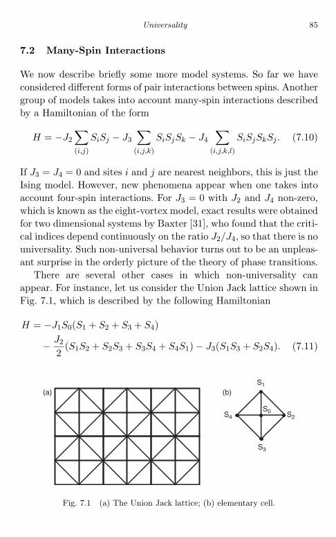
June 25, 2004 14:18 WSPC/Book Trim Size for 9in x 6in chap07
Universality 85
7.2 Many-Spin Interactions
We now describe briefly some more model systems. So far we haveconsidered different forms of pair interactions between spins. Anothergroup of models takes into account many-spin interactions describedby a Hamiltonian of the form
H = −J2∑(i,j)
SiSj − J3∑
(i,j,k)
SiSjSk − J4∑
(i,j,k,l)
SiSjSkSj . (7.10)
If J3 = J4 = 0 and sites i and j are nearest neighbors, this is just theIsing model. However, new phenomena appear when one takes intoaccount four-spin interactions. For J3 = 0 with J2 and J4 non-zero,which is known as the eight-vortex model, exact results were obtainedfor two dimensional systems by Baxter [31], who found that the criti-cal indices depend continuously on the ratio J2/J4, so that there is nouniversality. Such non-universal behavior turns out to be an unpleas-ant surprise in the orderly picture of the theory of phase transitions.
There are several other cases in which non-universality canappear. For instance, let us consider the Union Jack lattice shown inFig. 7.1, which is described by the following Hamiltonian
H = −J1S0(S1 + S2 + S3 + S4)
− J2
2(S1S2 + S2S3 + S3S4 + S4S1) − J3(S1S3 + S2S4). (7.11)
(a) (b)S1
S0 S2S4
S3
Fig. 7.1 (a) The Union Jack lattice; (b) elementary cell.

June 25, 2004 14:18 WSPC/Book Trim Size for 9in x 6in chap07
86 Phase Transitions
The factor 12 in the second term of Eq. (7.11), like that in Eq. (5.16),
takes into account the fact that each of the corresponding interactionsappears twice, in two adjacent cells. The particular cases, J1 = J3 = 0and J2 = J3 = 0, correspond to the nearest-neighbor Ising model.Moreover, when J3 = 0 and both J1 and J2 are non-zero, the exactsolution [32] again exhibits the Ising type critical behavior. How-ever, it has been shown [33] that the inclusion of an additional next-nearest-neighbor interaction J3, the value of which is determined byJ1 and J2, leads to non-universal eight-vortex type behavior.
Although the last example seems to be quite artificial, new typesof phase transitions may appear for models with competing two-spininteractions. So far we have considered only one type of interactionin any given system, ferromagnetic for J > 0, and antiferromag-netic for J < 0. However, the possibility exists that in some systemsthe interactions are competing. For instance the interaction betweennearest neighbors can be ferromagnetic and that between next near-est neighbors antiferromagnetic. In the next chapter we will considerthe so-called spin glasses, which are characterized by such competinginteractions.
7.3 Gaussian and Spherical Models
The discrete Ising models with two-spin interactions can be general-ized by other means. Two such models, the Gaussian model and thespherical model, were introduced by Mark Kac, to join “the small andselect company of models in statistical mechanics which can be rigor-ously discussed” [34]. In both of these models instead of the spins Sj
having a finite number of discrete values (±1 in Ising model), they arecontinuous variables that can have any real value (−∞ < Sj < ∞).The similarity of these models to the Ising model is as follows. Forthe Gaussian model, it lies in the additional requirements that foreach spin
〈S2j 〉 = 1. (7.12)
The condition (7.12) is a “relaxed” version of the “strong” conditionS2
j = 1 in the Ising model. The spherical model is closer to the Ising
June 25, 2004 14:18 WSPC/Book Trim Size for 9in x 6in chap07
Universality 87
model than the Gaussian model in that not only must Eq. (7.12) besatisfied, but there is also the overall restriction
N∑j=1
Sj = N. (7.13)
Both conditions (7.12) and (7.13) are obviously fulfilled in the Isingmodel.
Let us start with the Gaussian model. A Gaussian distribution ofthe spin variables is assumed, with 〈Sj〉 = 0 and 〈S2
j 〉 = 1, so thatthe probability P (Sj) dSj of finding a value Sj of the spin betweenSj and Sj + dSj is given by
P (Sj) dSj =1√2π
exp(
−12S2
j
)dSj . (7.14)
Then, the partition function Z has the following form
Z =(
12π
)N2
∫ ∞
−∞· · ·
∫ ∞
−∞dS1 · · · dSN
× exp(
−12
∑j
S2j +
J
kT
∑(i,j)nn
SiSj
). (7.15)
The integration in Eq. (7.15) can be easily performed using Eq. (7.5),and the result leads to the conclusion that the Gaussian model doesnot show a phase transition in any number of spatial dimensions.This result is not so surprising, since after transforming the integralin Eq. (7.15) to “normal coordinates” the partition function doesnot contain any interaction between these coordinates, and in sucha system without interactions there are no phase transitions in anynumber of spatial dimensions.
For the spherical model, the integration in Eq. (7.15) has to beperformed under the additional constraint (7.13) which can be writ-ten in the form of the delta function, δ
( ∑Nj=1 S2
j −N). If the integral
June 25, 2004 14:18 WSPC/Book Trim Size for 9in x 6in chap07
88 Phase Transitions
representation of the delta function
δ
( ∑j
S2j − N
)= (2π)−1
∫ ∞
−∞exp
[iu
( ∑j
S2j − N
)]du (7.16)
is substituted in Eq. (7.15), the following form of the partition func-tion is obtained for the spherical model:
Z =(
12π
)N2 +1 ∫ ∞
−∞du
∫ ∞
−∞· · ·
∫ ∞
−∞dS1 · · · dSN
× exp[iu
( ∑i
S2i − N
)−
∑j
S2j
2+
J
κT
∑(i,j)nn
SiSj
]. (7.17)
Once again the transformation (7.5) can be used to perform inte-grations over Sj , just at was done for the Gaussian model, and theremaining integral over u, for the large values of N in which we areinterested, can be carried out by the method of steepest descent. Itturns out that a phase transition in the spherical model occurs forthree and higher dimensional systems with critical indices differentfrom those of the Ising model [35].
A geometric picture helps to clarify the relation between the Ising,Gaussian and spherical models [36]. If one considers each Sj as acomponent of an N -dimensional vector, then the Gaussian modelcorresponds to integration throughout space, the spherical model tointegration over a spherical shell of radius
√N, and the Ising model
to summation over the corners of the unit hypercube inscribed withinthe unit sphere.
7.4 The x–y Model
We now turn to a model with properties very different from the aboveones, namely the x–y model, for which the Hamiltonian is
H = −J∑
(i,j)nn
(Sxi Sx
j + Syi Sy
j ) (7.18)
which corresponds to the generalized Heisenberg Hamiltonian ofequation (7.3) with J ′ = 0. This model, with a two-component order

June 25, 2004 14:18 WSPC/Book Trim Size for 9in x 6in chap07
Universality 89
parameter, is equivalent to one with ψ = ψ0eiθ, since one can write
Sxi = ψ0 cos(θi) and Sy
i = ψ0 sin(θi), where θi is the polar angle. Dueto the common multiplier J in Eq. (7.18), we can put ψ0 = 1. Then
H = −J∑
(i,j)nn
(cos θi cos θj + sin θi sin θj)
= −J∑
(i,j)nn
cos(θi − θj). (7.19)
For low temperatures the argument of the cosine is small, and so wecan expand it in terms of θi − θj . Then, apart from a constant term,the Hamiltonian (7.19) takes the following form
H =J
2
∑(i,j)nn
(θi − θj)2. (7.20)
Since the Hamiltonian (7.20) is a function of the polar angle θ, it isinvariant under the transformation
θi → θi + 2π. (7.21)
We now go from the lattice model, in which the angle θj is defined onthe sites j of a crystal lattice, to the continuous argument r, θ = θ(r).Then, the Hamiltonian (7.20) becomes
H =J
2
∫|∇θ (r)|2 ddr. (7.22)
Let us consider the correlation function g(r1 −r2) of the phase of theorder parameter
g(r1 − r2) =∫
expi[θ(r1) − θ(r2)] exp
[−J
∫ |∇θ (r)|2 ddr
2kT
]dθ.
(7.23)Using the (real) Fourier transform of θ(r):
θ (r) =∑K
[φK cos(K · r) + ζK sin(K · r)] (7.24)

June 25, 2004 14:18 WSPC/Book Trim Size for 9in x 6in chap07
90 Phase Transitions
one can rewrite Eq. (7.23) as
g(R) =∫∫
dφKdζK exp∑K
[AKφK + BKζK − JK2
2kT
(φ2K + ζ2
K)]
(7.25)where R = r1 − r2 and
AK = cos(K · r1) − cos(K · r2), BK = sin(K · r1) − sin(K · r2).(7.26)
On going from a sum over K in the exponent of Eq. (7.25) to anintegral in d dimensions, and completing the squares in φK and ζK,
one finds finally that
g(R) = exp
−kT
2J
∫ddK
K2 sin2(
KR
2
). (7.27)
It follows that for the different spatial dimensions d as R → ∞:
g(R) ∼ exp(
− R
Const
), d = 1;
g(R) ∼ Const · R−kT2πJ , d = 2; (7.28)
g(R) ∼ Const · exp(
ConstR
), d = 3.
In general, when R → ∞ the correlation function g(R) for a disor-dered system will decay exponentially, while in a completely orderedstate it will be constant, showing the presence of long range corre-lations. It follows from Eq. (7.28) that there is no phase transitionin a one-dimensional system while in three dimensions the systemhas long-range correlations. However, for d = 2 the correlation func-tion has a power law decay, which corresponds neither to order norto disorder, but rather to what is called quasi-order. Our calcula-tion represents a special case of the general Mermin–Wagner theo-rem about the absence of a phase transition in a one-dimensionaland a two-dimensional Heisenberg model [37]. In the last chapter wewill consider such a power-law dependence as a fingerprint of self-organized criticality in non-equilibrium systems. For the present, we
June 25, 2004 14:18 WSPC/Book Trim Size for 9in x 6in chap07
Universality 91
examine in more detail the two-dimensional x–y model, and compareit with the Landau mean field theory.
The order parameter η in the Landau theory can be written as
η = Ψ0 exp(iθ0).
In the standard (with no fluctuations) Landau theory, Eq. (3.6), aphase transition occurs at a temperature TL, and the amplitude ofthe order parameter Ψ0 in the ordered phase is equal to
√−A/(2B),while the phase θ0 is arbitrary. This theory ignores fluctuations, andso gives too low a value for the entropy S. According to Eq. (2.8), adecrease of entropy leads to an increase of the phase transition tem-perature. Thus, the critical temperature TL predicted by the Landautheory will be higher than that predicted by a theory that takes fluc-tuations into account. In order to include fluctuations in the Landautheory, we proceed as in Chapter 3, using the amplitude and thephase of the order parameter. We replace M in Eq. (3.19) by
ψ(r) = ψ0 + ψ1(r)eiθ(r),
where |ψ0|2 = − A2B as predicted by the Landau theory. Then
G = G0 −∫ [
2A |ψ1 (r)|2 − |∇ψ1 (r)|2]ddr
+ ψ20
∫|∇θ (r)|2)ddr + · · · . (7.29)
Just as in the calculations of Chapter 3, we use the Gaussian approxi-mation for fluctuations, and leave only quadratic terms in Eq. (7.29).The angular part of the Hamiltonian (7.29) is identical to the x–y
model (7.22). For high temperatures, T > TL, the system is in a dis-ordered state with exponentially decaying correlations. At T = TL,a non-zero amplitude of the order parameter appears, but there arestill fluctuations of the phase of the order parameter. Another phasetransition, the so-called Kosterlitz–Thouless phase transition occursat some temperature TKT smaller than TL, TKT < TL. This phasetransition is connected with the unbinding of vortices, which arebound in pairs for T < TKT , and become free for TKT < T < TL, asdiscussed below.

June 25, 2004 14:18 WSPC/Book Trim Size for 9in x 6in chap07
92 Phase Transitions
7.5 Vortices
The equilibrium states corresponding to the x–y Hamiltonian (7.22)can be obtained from the Lagrange equation
δH
δθ− ∇ δH
δ(∇θ)= 0 (7.30)
which for the x–y model reduces to
∇2θ = 0. (7.31)
For the two-dimensional case in which we are interested, the solutionof Eq. (7.31) has the form
∇θ =1r, θ = ln(r). (7.32)
The non-physical singularity of the function θ (r) at r = 0 can beremoved by cutting out a small circle of radius a near the origin.This means that one includes a special type of fluctuation with zeroorder parameter in the small region surrounding r = 0. Such exci-tations around the equilibrium state are called topological chargesor vortices, and the region 0 < r < a is called the core of the vor-tex. Vortices are characterized by their winding numbers, which aredefined as follows. Consider the integral
∮ ∇θ · dr around any closedpath enclosing the origin r = 0. Each circuit around the origin will,according to the symmetry property (7.21), bring us back to theoriginal system with an increase of 2nπ in the value of θ,∮
∇θ · dr = 2πn. (7.33)
Here n, which is called the winding number of the vortex, is a positive(for vortices) or negative (for anti-vortices) integer, depending onwhether the rotation is clockwise or anti-clockwise.
To answer the question whether vortices will appear as resultof thermal fluctuations at temperature T , one has to calculate thechange in the free energy F = E−TS associated with the appearanceof vortices. It follows from Eq. (7.22) and (7.32) that the energy

June 25, 2004 14:18 WSPC/Book Trim Size for 9in x 6in chap07
Universality 93
required to produce a vortex is
E =J
2
∫ L
a|∇θ|2 d2r = πJ ln
(L
a
)(7.34)
where L is a linear dimension of the system. On the other hand,since a vortex can appear everywhere in the system, the entropy ofa vortex is
S = k ln(
πL2
πa2
)= 2k ln
(L
a
). (7.35)
Therefore if T > TKT = πJ/(2k), the free energy F = E − TS
is negative, so that the appearance of a single vortex is energeti-cally favorable. As we will see in the next section, for temperaturesT < TKT , the interaction between vortices results in the binding ofvortex–antivortex pairs.
Incidentally, there is another example of a topological chargewhich is quite well known, though not necessarily by this name. Thisis the case of domain walls in ferromagnetic materials, which separateregions having opposite magnetizations. The number of domain wallsincreases as the critical temperature is approached from below, andthe ferromagnetic–paramagnetic phase transition can be regarded asa topological one, originating from the proliferation of domain walls.
7.6 Interactions Between Vortices
The final point that we want to consider in connection with the x–y
model is the interaction between vortices, and how they annihilateeach other when the temperature is lowered below the Kosterlitz–Thouless temperature TKT . Using Stokes theorem, one can rewriteEq. (7.33) as ∮
∇θ · dr =∫
(∇ × ∇θ) · dS = 2πn. (7.36)
The second integral in Eq. (7.36) is identically zero unlessthere are singularities at isolated points r = ri within the contour,

June 25, 2004 14:18 WSPC/Book Trim Size for 9in x 6in chap07
94 Phase Transitions
in which case
(∇ × ∇θ) = 2πez
∑i
niδ(r − ri) ≡ 2πn(r) (7.37)
where ez is the unit vector perpendicular to the xy-plane. From thesetwo equations one finds that∫
n(r) · dS = n. (7.38)
Let us define the velocity v of the phase θ to be its spatial gradient∇θ, v ≡ ∇θ. Since any vector v can be expressed as the sum of alongitudinal part vl and a transverse part vt,
v = vl + vt,
where ∇ · vt = 0 and ∇ × vl = 0, we assume such a division for v,and so consider only vt, for which ∇ × vt = 2πn(r) and ∇ · vt = 0,so that
∇ × (∇ × vt) = −∇2vt = 2π∇ × n(r). (7.39)
We solve this equation using the Green’s function G(r − r′) for theoperator ∇2, i.e., the solution of
∇2G(r − r′) = −δ(r − r′) (7.40)
which for a two dimensional system is given by
G(r − r′) =12π
ln( |r − r′|
a
). (7.41)
Then, the solution of Eq. (7.39) can be written as
vt (r) = −2π
∫d2r′G(r − r′)
[∇ × n(r′)]
= −2π
∫d2r′n(r′) × ∇G(r − r′). (7.42)
by using the standard formula for ∇×(Gn) and Stokes’ theorem. Theenergy of the system of vortices, U, is obtained by the substitution
June 25, 2004 14:18 WSPC/Book Trim Size for 9in x 6in chap07
Universality 95
of Eq. (7.42) into Eq. (7.22), which gives
U = 2π2J
∫drdr′dr′′[∇G(r − r′) × n(r′)] · [∇G(r − r′′) × n(r′′)].
(7.43)
On performing the partial integration over r and using Eq. (7.40)and (7.41), one finds that
U = πJ
∫dr′dr
′′ln
( |r′−r′′|a
)n
(r′) n(r′′). (7.44)
This equation, which describes the energy U of interaction betweentwo vortices, can be compared to the energy E of an individual vortexgiven by Eq. (7.34). While E is positive and diverges logarithmicallywith the size L of the system, the interaction energy U is negative forthe vortex–antivortex pair. Thus, if single vortices and antivorticeswere to appear at low temperatures, T < TKT , they would immedi-ately bind together. As we have seen earlier, only for temperaturesT > TKT does the appearance of individual vortex becomes ener-getically favorable. Without going into any further details, we onlynote [38] that for the topological Kosterlitz–Thouless phase transi-tion the correlation length ξ is always infinite below TKT , while aboveTKT it diverges according to the non-trivial law,
ξ ∼ exp(Const/√
T − TKT ).
Note the clear analogy between the behavior of vortices and that ofthe two-dimensional Coulomb gas with charges n and their interac-tion described by Eq. (7.44). In electrostatic language, the Kosterlitz–Thouless transition is analogous to unbinding the dipoles into singlecharges (a sort of insulator–metal transition).
7.7 Vortices in Superfluids and Superconductors
The x–y model is isomorphic to the superfluid and superconductingtransitions, where the two-dimensional order parameter describes thewave functions of the Bose–Einstein condensate and of the Cooperpairs, respectively, while the interaction energy J has to be replaced

June 25, 2004 14:18 WSPC/Book Trim Size for 9in x 6in chap07
96 Phase Transitions
by the superfluid density or by the electrical resistance of the two-dimensional films. In a three-dimensional superconductor, the pres-ence of an external magnetic field will make the system effectively twodimensional in the plane perpendicular to the field. The discovery ofthe high temperature superconductors stimulated a huge interest inthe theory of vortices, since these materials are type II superconduc-tors where the magnetic fields enters the superconducting materialsin the form of vortices. We refer the reader to the current scientificliterature for further details. As a starting point, one can use thecomprehensive reviews of the theory of vortices in superfluids andsuperconductors [39,40].
7.8 Conclusion
The Ising model can be extended to include many-spin interactions,which can lead to drastic changes of its properties, and, in particu-lar, to a dependence of the critical indices on the interaction energies(non-universality). The Ising model, as such, is a special case of themore general Heisenberg model, which for the three-dimensional casegives a phase transition with critical indices different from those ofthe Ising model. Another particular case of the Heisenberg model isthe x–y model, with vortices as an essential part of it. The latter playa crucial role in the modern theory of superfluidity and superconduc-tivity. Another pair of soluble models are the Gaussian and sphericalmodels, with the critical indices in the spherical model different fromthose in other models. Nevertheless, all these models can be arrangedby dividing them into a few universality classes. The university classto which a system belongs is specified by the following three factors:
(1) The spatial dimension d. In this respect, the lower critical dimen-sions, i.e., the minimum dimensions for the occurrence of phasetransitions, are two for the Ising and three for the Heisenbergmodel. The upper critical dimension for these models is four.Indeed, for four and higher dimensions the phase transitions aredescribed by mean field theory, with its own universality class.

June 25, 2004 14:18 WSPC/Book Trim Size for 9in x 6in chap07
Universality 97
(2) The dimension (number of components) D of the order param-eter. This dimension is unity for the Ising model and three forthe Heisenberg model, and so these two models lead to differentcritical behavior in three-dimensional systems.
(3) The finite or infinite radius of the interaction. In the latter case,each object interacts with all the others in the system, and onecan neglect fluctuations (a situation similar to that in high-dimensional systems) which immediately leads to the mean fielduniversality class.
All other factors, which define the short-range behavior (number ofstates at each site, type of the crystal lattice, etc.) of the system, donot influence the critical behavior.

This page intentionally left blank
June 25, 2004 14:18 WSPC/Book Trim Size for 9in x 6in chap08
Chapter 8
Random and Small World Systems
Most of the systems that we have considered so far in this bookhave been ordered ones, with definite well-defined spatial arrange-ments and interactions. In this chapter, we consider the effects ofdisorder or randomness. We consider first a simple example of a dis-ordered or random system, namely that of a lattice in which thereis a given probability that a bond exists between a pair of adjacentsites. Although the presence or absence of a bond is a purely geo-metrical property, with no thermal effects involved, this system isfound to have many features similar to those of a phase transition,such as a critical fraction of bonds for percolation to occur, criticalindices, and the applicability of renormalization group techniques,and so we consider it first. In fact, it is formally possible (althoughnot very instructive) to map the bond percolation problem on to thePotts model [36] mentioned in Chapter 7. After this we consider theIsing model with random interactions or sites removed at random,and spin glasses, in which there are competing interactions. Finally,we consider small world systems, in which there are a limited numberof long-range interactions between randomly chosen sites.
8.1 Percolation
The conceptually simplest example of a random system is a latticeof sites linked by bonds between adjacent sites in which a fraction x
of the bonds is removed at random. In such a system, the disorder orrandomness is uniquely specified by a single parameter, the fraction
99
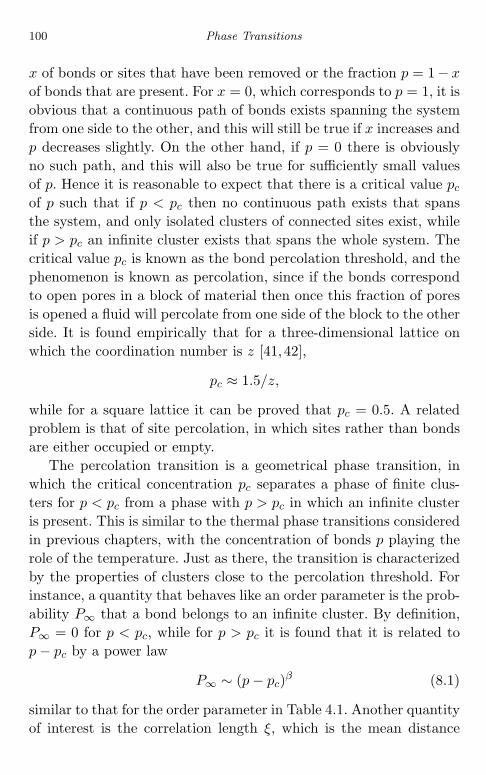
June 25, 2004 14:18 WSPC/Book Trim Size for 9in x 6in chap08
100 Phase Transitions
x of bonds or sites that have been removed or the fraction p = 1 − x
of bonds that are present. For x = 0, which corresponds to p = 1, it isobvious that a continuous path of bonds exists spanning the systemfrom one side to the other, and this will still be true if x increases andp decreases slightly. On the other hand, if p = 0 there is obviouslyno such path, and this will also be true for sufficiently small valuesof p. Hence it is reasonable to expect that there is a critical value pc
of p such that if p < pc then no continuous path exists that spansthe system, and only isolated clusters of connected sites exist, whileif p > pc an infinite cluster exists that spans the whole system. Thecritical value pc is known as the bond percolation threshold, and thephenomenon is known as percolation, since if the bonds correspondto open pores in a block of material then once this fraction of poresis opened a fluid will percolate from one side of the block to the otherside. It is found empirically that for a three-dimensional lattice onwhich the coordination number is z [41, 42],
pc ≈ 1.5/z,
while for a square lattice it can be proved that pc = 0.5. A relatedproblem is that of site percolation, in which sites rather than bondsare either occupied or empty.
The percolation transition is a geometrical phase transition, inwhich the critical concentration pc separates a phase of finite clus-ters for p < pc from a phase with p > pc in which an infinite clusteris present. This is similar to the thermal phase transitions consideredin previous chapters, with the concentration of bonds p playing therole of the temperature. Just as there, the transition is characterizedby the properties of clusters close to the percolation threshold. Forinstance, a quantity that behaves like an order parameter is the prob-ability P∞ that a bond belongs to an infinite cluster. By definition,P∞ = 0 for p < pc, while for p > pc it is found that it is related top − pc by a power law
P∞ ∼ (p − pc)β (8.1)
similar to that for the order parameter in Table 4.1. Another quantityof interest is the correlation length ξ, which is the mean distance

June 25, 2004 14:18 WSPC/Book Trim Size for 9in x 6in chap08
Random and Small World Systems 101
between two sites in a finite cluster. For p close to pc, this is given by
ξ ∼ |p − pc|−ν (8.2)
which can be compared to the behavior of the correlation length inTable 4.1. Other quantities of importance having similar types ofbehavior include the mean number of bonds in a finite cluster, thedistribution of finite clusters of different sizes, and for p > pc theprobability that a bond belongs to the infinite cluster. The problemof percolation, and especially in a continuum, is of great practicalimportance in many fields, such as the conductivity of a mixture ofconductors and insulators and the extraction of oil from an oil-field.A comprehensive review of the percolation transition and its rela-tionship to thermal phase transitions was presented by Essam [43].
8.2 Ising Model with Random Interactions
So far, we have considered the Ising model
H = −∑
(i,j)nn
JijSiSj (8.3)
with uniquely specified values for the interactions Jij between thespins on different sites. When these interactions are all ferromag-netic, Jij = J > 0, the equilibrium state at any given temperatureis uniquely defined, and if a phase transition occurs, it is between awell-ordered state and a disordered one, with a change of the sym-metry of the system at the phase transition point. The Ising modelwith an antiferromagnetic interaction, i.e., with Jij = J < 0, usuallyhas similar properties. However, for certain types of lattice, there isnot a unique equilibrium state at low temperatures because of frus-tration. The simplest example of frustration is the antiferromagnetictriangular lattice in two dimensions. Let us consider three mutuallyadjacent atoms, A, B, and C. If the spin at site A is up, the inter-action favors the spins at sites B and C to both be down, while theinteraction between the spins at B and C wants them to be of oppo-site sign. We now examine the Ising model for random systems, in
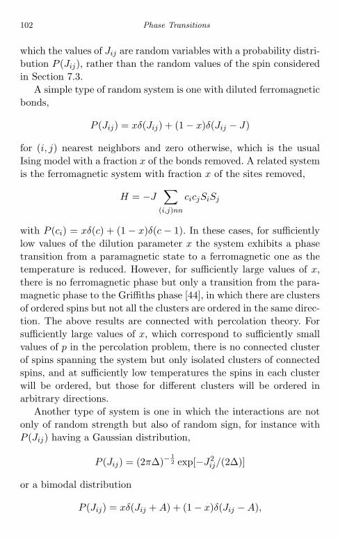
June 25, 2004 14:18 WSPC/Book Trim Size for 9in x 6in chap08
102 Phase Transitions
which the values of Jij are random variables with a probability distri-bution P (Jij), rather than the random values of the spin consideredin Section 7.3.
A simple type of random system is one with diluted ferromagneticbonds,
P (Jij) = xδ(Jij) + (1 − x)δ(Jij − J)
for (i, j) nearest neighbors and zero otherwise, which is the usualIsing model with a fraction x of the bonds removed. A related systemis the ferromagnetic system with fraction x of the sites removed,
H = −J∑
(i,j)nn
cicjSiSj
with P (ci) = xδ(c) + (1 − x)δ(c − 1). In these cases, for sufficientlylow values of the dilution parameter x the system exhibits a phasetransition from a paramagnetic state to a ferromagnetic one as thetemperature is reduced. However, for sufficiently large values of x,there is no ferromagnetic phase but only a transition from the para-magnetic phase to the Griffiths phase [44], in which there are clustersof ordered spins but not all the clusters are ordered in the same direc-tion. The above results are connected with percolation theory. Forsufficiently large values of x, which correspond to sufficiently smallvalues of p in the percolation problem, there is no connected clusterof spins spanning the system but only isolated clusters of connectedspins, and at sufficiently low temperatures the spins in each clusterwill be ordered, but those for different clusters will be ordered inarbitrary directions.
Another type of system is one in which the interactions are notonly of random strength but also of random sign, for instance withP (Jij) having a Gaussian distribution,
P (Jij) = (2π∆)− 12 exp[−J2
ij/(2∆)]
or a bimodal distribution
P (Jij) = xδ(Jij + A) + (1 − x)δ(Jij − A),

June 25, 2004 14:18 WSPC/Book Trim Size for 9in x 6in chap08
Random and Small World Systems 103
frequently studied for the symmetric case x = 12 . In systems with
such combinations of ferromagnetic and anti-ferromagnetic interac-tions, frustration of the spins occurs, similar to that mentioned abovefor the antiferromagnetic Ising model on a triangular lattice. As aresult, these systems, which are known as spin glasses, have no uniqueground state.
8.3 Spin Glasses
There are a variety of magnetic systems in nature that behave asspin glasses. One type is that of magnetic ions such as iron or cobaltinserted as substitutional impurities at random sites in a lattice ofnon-magnetic metal ions such as copper. These systems have frozendisorder, similar to that of a glass at low temperatures, and theinteractions between the spins on the magnetic ions are indirect, i.e.,they are mediated by the spins of the electrons attached to the hostatoms or by free electrons. In the latter case, there is an effectivemagnetic interaction of the Ruderman–Kittel form [45]
φ(r) = φ0 sin(kF r)/(kF r)3,
where kF is the wave number of electrons on the Fermi surface, sothat the sign of this interaction varies with the distance r betweenthe magnetic ions.
A major difference exists between ferromagnetic system and spinglasses with respect to their symmetry properties. In ferromagneticmaterials, when the temperature is raised through Tc the equilibriumstate of the system changes to the paramagnetic one, with a suddenchange in the magnetic moment M and symmetry breaking. More-over, in ferromagnetic systems such as the original Ising model, attemperatures T < Tc the system is ferromagnetic, with all the spinspointing in the same direction, and there is degeneracy between thestates with all spins up and all spins down. In the thermodynamiclimit, these two states are separated by an infinite potential barrier,so that no transition between them can occur. As a result, in theferromagnetic state not all states in phase space are allowed. Since

June 25, 2004 14:18 WSPC/Book Trim Size for 9in x 6in chap08
104 Phase Transitions
a system is ergodic only when it is free to sample all points in phasespace, this means that the ergodicity is broken at Tc. Incidentally,the degeneracy of the ferromagnetic state can be removed (in orderto produce a unique ground state) by applying a small magnetic fieldor by introducing suitable boundary conditions. Thus, for ferromag-netic systems, both symmetry and ergodicity are broken at Tc. Inspin glasses, by contrast, while there is a critical temperature Tc, themean magnetic moment 〈M〉 is zero both below and above it, andthe transition is characterized by a cusp-like singularity of the sus-ceptibility at Tc [46]. Below the critical temperature there are manycompeting ground states, separated by infinite barriers. This meansthat for spin glasses the ergodicity is broken at Tc (as a result offrustration), but this broken ergodicity is not accompanied by bro-ken symmetry.
In all random systems, the macroscopic properties are those of aconfigurational average of the system, which we denote by 〈· · ·〉, i.e.,the property has to be calculated separately for each possible acces-sible configuration of the system and an average taken (with theappropriate weights of the probability of that configuration beingfound) over all the possible configurations. In general, there are twotypes of random system, annealed or quenched, depending on therate of change of the disorder, for instance as a result of the mobil-ity of magnetic ions in spin glasses. In annealed systems this rate isfast, so that one requires the average of the positions of the impuri-ties which enter the partition function, and one has to average thepartition function 〈Z〉. On the other hand, in quenched systems thisrate is slow and the disorder is essentially fixed, so that one has tominimize, the free energy F = −kT lnZ individually for each pos-sible configuration, and so the important quantity is 〈lnZ〉. In spinglasses the disorder is quenched, so that for the macroscopic systemone has to average over the free energy for different configurationsrather than over the partition function. This is the main problem inthe theoretical analysis of spin-glasses.
There are two well-known models for spin glasses, the “short-range” Edwards–Anderson and the “infinite-range” Sherrington–Kirkpatrick models, which overcome the difficulty stemming from

June 25, 2004 14:18 WSPC/Book Trim Size for 9in x 6in chap08
Random and Small World Systems 105
the nonlinearity of the logarithm function appearing in the expres-sion for the quenched free energy by the so-called replica method [47]based on the self-evident identity,
lnZ = limn→0
Zn − 1n
. (8.4)
Equation (8.4) means that one can calculate the quenched averagefree energy by creating multiple copies of the system, averaging them,and then letting the number of copies tend to zero. The calculationof Zn is similar to that performed in Chapter 7 for the sphericalmodel, but with many delicate points, such as the meaning of thelimit n → 0, its interchange with the thermodynamic limit, etc.
There are a number of problems from different fields that can berelated to the spin glass problem, and we will mention two of them.The theory of spin glasses can be used to derive computer algorithmsfor the solution of optimization problems, such as that of the trav-elling salesman [48] (who has a large number of possible routes, andif he spends all his time trying to work out the best one he willnever sell anything). Another problem related to spin glasses is thatof neurons in the brain, which can be in one of two states (“firing” or“non-firing”), just like the spins in the Ising model. An appropriatemodel to describe the possible patterns of neural connections wasintroduced by Hopfield [49], and has led to an enormous amount ofwork on neural networks, with applications to understanding suchfunctions of the brain as learning, and to attempts to mimic them soas to obtain self-correcting systems.
8.4 Small World Systems
We are living in a large world, and already in 1999 the populationof the Earth exceeded six billion people. On the other hand, if wesuddenly meet our neighbor somewhere in the Amazon jungle, weexclaim: “This is a small world!”. The simple “large-small” gamescan be illustrated by the Bacon and Erdos numbers. The famousactor Kevin Bacon played in many movies with different actors, whocan thereby be characterized by their different Bacon numbers, where
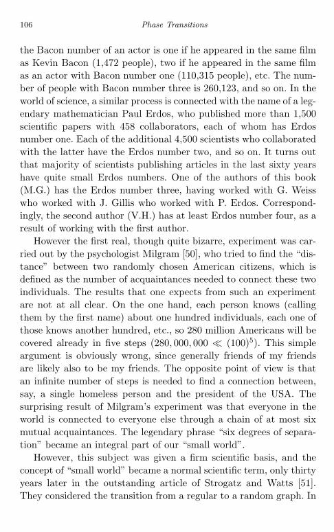
June 25, 2004 14:18 WSPC/Book Trim Size for 9in x 6in chap08
106 Phase Transitions
the Bacon number of an actor is one if he appeared in the same filmas Kevin Bacon (1,472 people), two if he appeared in the same filmas an actor with Bacon number one (110,315 people), etc. The num-ber of people with Bacon number three is 260,123, and so on. In theworld of science, a similar process is connected with the name of a leg-endary mathematician Paul Erdos, who published more than 1,500scientific papers with 458 collaborators, each of whom has Erdosnumber one. Each of the additional 4,500 scientists who collaboratedwith the latter have the Erdos number two, and so on. It turns outthat majority of scientists publishing articles in the last sixty yearshave quite small Erdos numbers. One of the authors of this book(M.G.) has the Erdos number three, having worked with G. Weisswho worked with J. Gillis who worked with P. Erdos. Correspond-ingly, the second author (V.H.) has at least Erdos number four, as aresult of working with the first author.
However the first real, though quite bizarre, experiment was car-ried out by the psychologist Milgram [50], who tried to find the “dis-tance” between two randomly chosen American citizens, which isdefined as the number of acquaintances needed to connect these twoindividuals. The results that one expects from such an experimentare not at all clear. On the one hand, each person knows (callingthem by the first name) about one hundred individuals, each one ofthose knows another hundred, etc., so 280 million Americans will becovered already in five steps (280, 000, 000 (100)5). This simpleargument is obviously wrong, since generally friends of my friendsare likely also to be my friends. The opposite point of view is thatan infinite number of steps is needed to find a connection between,say, a single homeless person and the president of the USA. Thesurprising result of Milgram’s experiment was that everyone in theworld is connected to everyone else through a chain of at most sixmutual acquaintances. The legendary phrase “six degrees of separa-tion” became an integral part of our “small world”.
However, this subject was given a firm scientific basis, and theconcept of “small world” became a normal scientific term, only thirtyyears later in the outstanding article of Strogatz and Watts [51].They considered the transition from a regular to a random graph. In
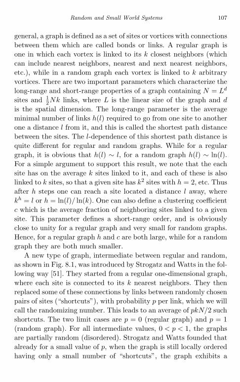
June 25, 2004 14:18 WSPC/Book Trim Size for 9in x 6in chap08
Random and Small World Systems 107
general, a graph is defined as a set of sites or vortices with connectionsbetween them which are called bonds or links. A regular graph isone in which each vortex is linked to its k closest neighbors (whichcan include nearest neighbors, nearest and next nearest neighbors,etc.), while in a random graph each vortex is linked to k arbitraryvortices. There are two important parameters which characterize thelong-range and short-range properties of a graph containing N = Ld
sites and 12Nk links, where L is the linear size of the graph and d
is the spatial dimension. The long-range parameter is the averageminimal number of links h(l) required to go from one site to anotherone a distance l from it, and this is called the shortest path distancebetween the sites. The l-dependence of this shortest path distance isquite different for regular and random graphs. While for a regulargraph, it is obvious that h(l) ∼ l, for a random graph h(l) ∼ ln(l).For a simple argument to support this result, we note that the eachsite has on the average k sites linked to it, and each of these is alsolinked to k sites, so that a given site has k2 sites with h = 2, etc. Thusafter h steps one can reach a site located a distance l away, wherekh = l or h = ln(l)/ ln(k). One can also define a clustering coefficientc which is the average fraction of neighboring sites linked to a givensite. This parameter defines a short-range order, and is obviouslyclose to unity for a regular graph and very small for random graphs.Hence, for a regular graph h and c are both large, while for a randomgraph they are both much smaller.
A new type of graph, intermediate between regular and random,as shown in Fig. 8.1, was introduced by Strogatz and Watts in the fol-lowing way [51]. They started from a regular one-dimensional graph,where each site is connected to its k nearest neighbors. They thenreplaced some of these connections by links between randomly chosenpairs of sites (“shortcuts”), with probability p per link, which we willcall the randomizing number. This leads to an average of pkN/2 suchshortcuts. The two limit cases are p = 0 (regular graph) and p = 1(random graph). For all intermediate values, 0 < p < 1, the graphsare partially random (disordered). Strogatz and Watts founded thatalready for a small value of p, when the graph is still locally orderedhaving only a small number of “shortcuts”, the graph exhibits a

June 25, 2004 14:18 WSPC/Book Trim Size for 9in x 6in chap08
108 Phase Transitions
Fig. 8.1 Three types of graphs: regular, random and regular with a small numberof “shortcuts” (small world). Reprinted by permission from Nature [51] copyright2003, Macmillan Publishers Ltd.
different behavior, namely h(l) ∼ ln(l), as in random graphs, but c
remains close to unity, similar to regular graphs. Such a behavior isknown as “small world” [51]. The drop in h from h ∼ l to h ∼ ln(l) isconnected with the small number of shortcuts which bring togetherpreviously distant sites.
Now that we have three types of graph, regular (“large world”),disordered (“small world”) and random, we have to decide which typeis most common in real life. To do this, it is convenient to changeour terminology, and assume that the sites in the graphs are occupiedby some objects, and that links correspond to interactions betweenthese objects. These new systems will be called networks. The con-cept of networks is very general, and incorporates such systems asinteracting atoms and galaxies, different groups of people, sites on theInternet, etc. In their original article Strogatz and Watts consideredthree different networks (a sociological system of film actors, a biolog-ical system of the worm’s neural network, and the man-made powergrid in the western US), and found that all of them exhibit the smallworld phenomena. A more recent development is that many othernetworks belong to the small world category (see Watts’ book [52]and some recent reviews [53,54]). In addition to the topological char-acteristics h and c of the network, some new parameters (efficiencyand cost, geographic distances [55], etc.) have been introduced forthe description of real networks.

June 25, 2004 14:18 WSPC/Book Trim Size for 9in x 6in chap08
Random and Small World Systems 109
8.5 Evolving Graphs
So far we have examined graphs with a fixed number of sites andlinks. However, most real systems are “living”, i.e., their size L
changes with time. Accordingly, let us consider graphs which arecharacterized by three parameters, the number k of closest neigh-bors, the randomizing number p, and the total number of sites Ld.In the previous section we considered the p-dependence of two char-acteristic parameters, the path length h(l) and the cluster coefficientc, provided that k and L remained constant. As we saw, the shortestpath distance h(l) between two sites distance l apart is quite differ-ent for regular and random graphs, being proportional to l and ln(l),respectively. The question arises as to the conditions for a transitionfrom one regime to another to take place, or in other words how largehas the disorder to be for a transition to take place from a regularlattice to a random one. Roughly speaking, a graph is regular whenthe fraction of random links Nrd is small, Nrd 1, and it is randomwhen this fraction is large, 1 − Nrd 1. The total number of linksis 1
2kLd, where d is the spatial dimension, and the probability of arandom link is p, so that the average fraction of random links Nrd
is given by Nrd = 12kLdp. Since Nrd is small for regular graphs and
close to unity for random ones, it seems natural to assume that thetransition occurs at some “crossover” size L∗ such that
Nrd =12kL∗dp =
12, (8.5)
i.e., the graph with given k and p is regular when L < L∗ and randomwhen L > L∗. The heuristic arguments which lead to Eq. (8.5) aresupported by the renormalization group analysis [56]. For a one-dimensional system, it follows that
L∗ ∼ 1p. (8.6)
We note that the transition from a regular to a random graph occursat some value L∗ of L no matter how small is the randomizing num-ber p. Moreover, an analogy exists between this “geometric” phasetransition and the “physical” phase transitions considered in previous
June 25, 2004 14:18 WSPC/Book Trim Size for 9in x 6in chap08
110 Phase Transitions
chapters, with L and p playing the role of the correlation length andthe dimensionless temperature, respectively. Later on we will com-pare the characteristic length L∗ with the correlation length ξ.
8.6 Phase Transitions in Small World Systems
In the previous section we considered the “geometric” phase tran-sition controlling the transition from regular to random graphs.There are, however, also “physical” phase transitions, if the smallworld defines the underlying topology for physical objects locatedon sites of these graphs, with the links defining the interactionsbetween these objects. In such a way we obtain physical objectswith random interactions. A simple example is provided by the Isingmodel applied to linear polymers, where the short-range interac-tions between neighboring monomers in the chain are supplementedby the random interactions between monomers that are close inspace (and not along the chain). This example demands a slightchange of the original model [51] in which the shortcuts do notreplace the short-range interactions but rather are added to them,i.e., no links are removed from the regular lattice but extra links areintroduced.
Let us recall the main results of the regular one-dimensional Isingmodel considered in Chapter 2. Such a system with N sites has nophase transition at finite temperatures in the thermodynamic limitN → ∞. However, a mean field type phase transition is found in theKac model [30] where, in addition to the short-range interactions, oneadds a large (of order of N2) number of weak interactions betweenall pairs of spins. The ferromagnetic one-dimensional Ising model hasbeen analyzed analytically and numerically in small world systems. Itis found from analytical calculations [57, 58] that a mean field tran-sition occurs at a finite temperature Tc(p) for any p > 0 providedthat the number of sites is large enough, and numerical simulationsshow that the critical indices have their mean field values [59]. Closeto p = 0 the transition temperature Tc goes to zero as | ln(p)|−1.
Hence, in order to obtain the mean field phase transition in a one-dimensional Ising system there is no need for long-range interactions

June 25, 2004 14:18 WSPC/Book Trim Size for 9in x 6in chap08
Random and Small World Systems 111
between all the spins, and it is enough to have a comparatively smallnumber of randomly chosen long-range interactions. We note that amean field type behavior has also been found by Monte Carlo sim-ulations for the x − y model based on two-dimensional small worldgraphs [60].
The problem becomes more interesting in two and three dimen-sions where phase transitions already occur in the ordered (p = 0)systems, and one expects that the appearance of a small amount ofdisorder (p 1) will result in a change of the universality class of thistransition from that of the Ising model for p = 0 to that of the meanfield for p > 0. If this change occurs at finite p, the question arisesas to the dependence of the critical indices on p in the transitionregime. It turns out, however, that the transition to the mean-fieldtype behavior probably occurs for all p > 0, provided that the num-ber of sites is large enough, although numerical simulations [60, 61]have been restricted to p ≥ 10−3. If this last statement is correct,the question arises as to the dependence on p of the transition tem-perature Tc for small p. An elegant answer to this question has beenfound by Herrero [61]. Let us compare the two characteristic lengthsappearing in our problem, the characteristic length L∗ which definesthe transition from regular (large world) to random (small world)behavior, and the correlation length ξ of the “physical” phase tran-sition. When ξ is smaller than L∗, the system behaves as a regularlattice. However, as the temperature decreases ξ becomes larger thanL∗, and so the random interactions become important and give rise tothe mean field behavior. Thus the transition between the regular lat-tice (Ising type behavior) and the small world (mean field behavior)occurs for ξ ≈ L∗. For the one-dimensional Ising model the corre-lation length at low temperature is given by ξ ∼ exp[2J/(kT )] [36],and for L∗ ∼ p−1, the condition ξ ∼ L∗ results in Tc ∼ | ln(p)|−1
in agreement with [58]. For higher dimensions, ξ ∼ |T − Tc,p=0 |−ν
and L∗ ∼ p−1/d. Thus, the change in the temperature of the phasetransition for a non-zero randomizing parameter p is given, for smallp, as
Tc − Tc,p=0 ∼ p1
νd . (8.7)
June 25, 2004 14:18 WSPC/Book Trim Size for 9in x 6in chap08
112 Phase Transitions
8.7 Conclusion
Although systems with random interactions have been studied formany years, especially in the framework of spin glass theory, a freshpoint of view was introduced a few years ago with the discovery ofsmall world phenomena. It turns out that most real “many-body”natural and human-made systems exhibit small world properties,having a short-range structure like that of ordered systems anda long-range structure similar to that of random systems. Theseunusual properties lead to many important applications in scienceand sociology [53,54].

June 25, 2004 14:19 WSPC/Book Trim Size for 9in x 6in chap09
Chapter 9
Self-Organized Criticality
Many-particle systems can be divided into two classes. On the onehand, one can start with a superficially simple system such as anatom, and then consider more and more complex systems as oneprobes further and further into its structure, electrons and a nucleus,the nucleus containing protons and neutrons, these being composedof quarks, and so on. On the other hand, one can consider large sys-tems that are inherently complex because they contain many objects,with very many degrees of freedom and a large number of connec-tions between them. Just as in the previous chapter, these systemscan be described in terms of networks of sites and bonds. Such anetwork can refer not only to the atoms or molecules in a solid or afluid but also to groups of people and their interactions, competingcompanies on the stock market, the sites and links of the Internet,and numerous other systems. In our analysis we consider those prop-erties which are independent of the type of objects located at thesites and connected by the bonds, but rather depend on the topo-logical properties of networks. Such properties are very appropriateto phase transitions, where as we saw in Chapter 7 the universalityclasses do not depend on the detailed properties of the objects beingassociated with the infinite correlation length.
In the previous chapter we classified networks by the parametersh and c. Another way of doing so is to introduce the probabilityP (l) ∼ l−δ that two sites at a distance l are connected. If δ = 0,P (l) is constant, so that links of all sizes are equally probable, asin the random graphs discussed in the previous chapter. On the
113

June 25, 2004 14:19 WSPC/Book Trim Size for 9in x 6in chap09
114 Phase Transitions
other hand, if δ is very large then long-range links are restricted,and one effectively obtain a regular graph with only short-rangelinks. For intermediate values of δ, one gets the original Strogarz–Watts model of a small world [51]. It turns out [62] that for δ < δ1
the system behaves as a random network, for δ1 < δ < δ2 thebehavior is of the small world type, and for δ > δ2 it behavesas a regular network, while for a one-dimensional system δ1 = 1and δ2 = 2.
For the probability of a connection between two sites, we intro-duced the power law distribution P (l) ∼ l−δ. In general, for inde-pendent random events with a finite mean a and variance σ, thecentral limit theorem states that a property x will have the Gaussiandistribution,
P (x) = (2πσ)− 12 exp[−(x − a)2/2σ].
This bell-shape curve distribution is probably the most common typeof figure in the scientific literature. As we have seen in the pre-vious chapters, in some special cases the Gaussian distribution isreplaced by a power-law one. The two examples that we examinedpreviously are the spatial dependence of the correlation function atcritical points and of the correlation length in the low temperatureregion of the x–y model. In contrast to these special cases of systemsin equilibrium, which only apply to some special temperature region,there is a wide class of non-equilibrium phenomena which are of thepower law type. Since these systems evolve spontaneously into criticalstates because of their internal dynamics, with no dependence on thevalue of an external parameter, their behavior is called self-organizedcriticality (SOC). An alternative name for such systems is scale-freesystems, since the power law distribution is scale-invariant and doesnot involve a characteristic length scale. This situation is similar tothat which occurs close to the critical points in equilibrium systems,where the short-range lengths are of no importance and the onlycharacteristic length is the correlation length. This diverges at thecritical point, so that there is no characteristic length at this point.

June 25, 2004 14:19 WSPC/Book Trim Size for 9in x 6in chap09
Self-Organized Criticality 115
9.1 Power Law Distributions
In considering power-law distributions, we start with some oldempirical laws. One of the oldest examples (1897) is the Pareto dis-tribution [63] describing the distribution of large wealth w in differ-ent societies. It turns out that the number of people N(w) havingwealth w, has a form N(w) ∼ w−α with α between 2 and 3. Veryrecently [64], the effects have been considered of using fiscal policyto change the value of α, and some surprising results have beeenfound with regard to the probability of an individual becoming verywealthy (wealth condensation). A similar power-law distribution wasfound by Guttenberg and Richter [65] in 1954 for the number N(E) ofearthquakes which release a certain amount of energy E. This depen-dence has the form N(E) ∼ E−α, with α = 1.5 independent of thegeographic region examined. Finally, in the 1930’s, Zipf found [66] thepower-law distributions of towns according to their populations andof the frequency of appearance of different words in the English lan-guage. There are many more systems with power-law distributions,such as climate fluctuations, cloud formation, rainfall, volcanic erup-tions, forest fires, commodity prices, scientific collaborations, cita-tions, the structure of the Internet web and traffic jams. One of themost recently found and exotic examples is the power-law distribu-tion of the wealth of the inhabitants of the ancient Egyptian cityAkhetaten, based on the excavations and on the assumption thatwealth was proportional to the house area [67].
The power-law distribution, unlike the Gaussian distribution, hasthe form of a straight line in a logarithmic plot and has no distinctivevalue. This feature has some interesting consequences, of which twoare of special importance. First of all, it is meaningless to define atypical income or the average strength of an earthquake, which wouldcorrespond to the peak of a Gaussian distribution. Secondly, and ofgreater importance, the straight line logarithmic distribution sug-gests that the same mechanism is responsible for earthquakes of allsizes, including the largest ones. Such large values are often regardedas exceptions, or catastrophic, but the power law distribution showsthat although they are rare in occurrence, they are expected to occur
June 25, 2004 14:19 WSPC/Book Trim Size for 9in x 6in chap09
116 Phase Transitions
occasionally, and do not require any special explanation. This maybe counter to our physical intuition, in which we are used to sys-tems in thermal equilibrium within deep potential minima, wherethe response is proportional to the disturbance. In that case, smalldisturbances lead to small consequences and some special mecha-nism is required to produce large effects. However, there are occa-sional exceptions even for systems in equilibrium. One example isthe divergent susceptibility at the critical point, which leads to asmall disturbance producing a large response near this point. In thismanner, the gravitational field, which in general is negligible for alllaboratory experiments, becomes important near the liquid-gas criti-cal point. Because of the infinite compressibility ∂ρ/∂p at the criticalpoint, even the small change in pressure δp along a vertical tube 10 cmlong leads to a large difference δρ ∼ (∂ρ/∂p)δp between the fluid’sdensity at the top and bottom of the tube (“gravity effect” [68]),which can be as large as 10%. Similarly, in systems driven at a fre-quency close to the system’s resonance frequency a small force canproduce a catastrophic response, as happened in the collapse of theTakoma Bridge on the 7th November 1940.
A basic difference between the above systems and those that weare considering now is that the latter are not in thermodynamicequilibrium. One can imagine, for example, a shallow valley in thepotential landscape, in which case only a small stimulus is requiredto lift the system out of this valley, and it can then fall into anotherpotential valley of arbitrary depth. A simple example of this is pro-vided by a man standing on a mountain. If he is at the bottom of themountain, a small push will have very little effect. If he is standingon a ridge which has a wider ridge slightly below it, then a smallpush will at most cause him to fall a short distance. However, if heis standing at the top of the mountain with a sheer drop to downbelow, then a small push away from the edge will have little effect,but a small push over the edge will have catastrophic results. Letus bring two illustrative examples of such catastrophic effects. Whileone can easily find the obvious reason for the crash of New Yorkstock exchange after 11th September 2001, it is very hard to find aspecial reasons for the “black Monday” of 19th October 1987, the
June 25, 2004 14:19 WSPC/Book Trim Size for 9in x 6in chap09
Self-Organized Criticality 117
greatest one-day crash in history, when that market lost 20% of itsvalue in one day. The second example concerns the disappearance ofdinosaurs. It is possible that this was due to the collision of Earthwith an asteroid, or due to a drastic change of the climate, or due to ahuge volcanic eruption. However, there may be no need for a specialexplanation, as this phenomena — the disappearance of dinosaurs —could have happened due to the internal properties of the ecosystem.
9.2 Sand Piles
The paradigm for power-law distributions, and the one which wasthe subject of the first serious theoretical studies, is provided by sandpiles. As grains of sand are dropped one by one, slowly and uniformly,onto a table, at first they stay where they land, forming an initial thinlayer, and then grains will accumulate on top of one another creatinga pile. However, this pile will not grow taller forever. At some stage,the sand pile will enter a state of self-organized criticality (SOC),with a slope of 34–37, and then a qualitative change will occur. Anew falling grain has the following three possibilities:
(1) It can fall to the bottom of the pile, and so enlarge the pile’sbase.
(2) It can stick to the side of the pile at some point, thereby increas-ing slightly the angle of slope of the pile.
(3) It may increase the angle of slope above a critical value and sotrigger an avalanche in which S grains fall to the bottom of thepile, some of which may have been located nowhere near the placewhere the grain which started the avalanche fell. This happensbecause in the SOC state the whole pile has become connected,so that even a single grain (small disturbance) in one part ofthe pile may trigger a large avalanches (catastrophic event) any-where else. In the SOC state the global dynamics controls thebehavior of the sand pile as a whole rather than that of the indi-vidual grains. In this SOC state the number N(S) of avalanchesinvolving S grains is found to have the power law distributionN(S) ∼ S−α with α ≈ 1. It is intuitively clear that there is no

June 25, 2004 14:19 WSPC/Book Trim Size for 9in x 6in chap09
118 Phase Transitions
typical size of an avalanche, and there are no obvious precursorsof a huge, catastrophic avalanche. Since each grain “knows” onlyits short-range environment, it does not expect to be involved inan avalanche, and no predictions of the catastrophic events canbe made.
For a mathematical model of such a process, one describes thesystem as a box which is divided into cells, and assumes that thereis an upper limit to the number of particles that can accumulate in asingle cell. When a cell contains this maximum permissible number ofparticles, the arrival of an additional particle will cause some particlesto leave it for other cells. If one or more of these particles move to cellswhich are located near the boundaries of the box and already containthe maximum number of particles, then more and more particles willleave the system creating thereby an avalanche.
A similar model can be used for study of forest fires. For the modelof a forest, the boxes consist of cells with trees inside them. Then,one of the trees is set on fire, and one studies how many trees will beconsumed before the fire extinguishes itself. A study of this systempermits the planning of how to plant forests in such a way as to min-imize the risks of large fires. It may be useful to initiate occasionallysmall fires so as to reduce the connections between different groupsof trees (cells), and kept the whole system below the critical SOClevel when fires of arbitrary size (including huge avalanches) becomepossible. It is possible that the wrong policy of keeping the ecosystemin its virgin form, and so suppressing the small fires, was responsiblefor not preventing the huge 1988 fire in Yellowstone National Parkin USA. The forest fire professionals now recognize that the best wayto prevent the largest fires is to allow small and medium size firesto burn.
9.3 Distribution of Links in Networks
As in the previous chapter, let us consider a network consisting of alarge number N of sites each having a number k links to other sites inthe network. Different sites may have different number of links, and

June 25, 2004 14:19 WSPC/Book Trim Size for 9in x 6in chap09
Self-Organized Criticality 119
so we introduce the probability distribution of the number k of links,P (k), where ki is the number of links (also called connectivities)of site i. For a scale free systems P (k) is the power law function,P (k) ∼ k−γ .
In order to show how a power-law distribution can appear, weassociate with each site i a random number xi[xi ∈ (0,∞)], whichwe call the rank of site i and use it to measure the importance of thissite [69]. Let f(x) be the probability distribution of the ranks, whichfor scale free systems we take to be a power law distribution similarto those considered previously in this chapter. In addition, we assumethat the probability that a link exists between a pair of sites i and j
is ψ(xi, xj). Incidentally, for random graphs, this probability is thesame for all sites coupled, and ψ(xi, xj) is a constant, ψ(xi, xj) = b.
The mean connectivity of a site of rank x is
〈k(x)〉 =∫ ∞
0ψ(x, y)f(y)dy ≡ NF (x) (9.1)
so that x = F−1( 〈k〉
N
). On the other hand, by definition
〈k〉 =∫ ∞
0kP (k)dk. (9.2)
On combining Eqs. (9.1) and (9.2), one obtains, using P (k) =f(x)dx/dk,
P (k) = f
[F−1
(〈k〉N
)]d
dk
[F−1
(〈k〉N
)]. (9.3)
As a special example, we consider ψ(xi, xj) = xixj/x2max, where xmax
is the largest rank in the network. Then,
〈k(x)〉 =Nx
x2max
∫ ∞
0yf(y)dy = N
x〈x〉x2
max(9.4)
and
P (k) =x2
max
N〈x〉f(
x2max
N〈x〉k)
. (9.5)

June 25, 2004 14:19 WSPC/Book Trim Size for 9in x 6in chap09
120 Phase Transitions
One sees from Eq. (9.5), that the distribution of connectivities P (k)is completely determined by the distribution of ranks f(x), so thatif f(x) is a power law distribution, then so is the distribution P (k)of connectivities.
9.4 Dynamics of Networks
So far we have considered only static networks. However, most net-works are not static, as the number of sites can change with time,new sites and links can appear, and some of the old ones may disap-pear. For instance, in the world wide web of the Internet, new sitesare continually being created, as are new links between sites, whilesome sites may also disappear. Similarly, in the financial world, newbusinesses are continually being created and others liquidated, whileassets are also transferred from one firm to another.
The main assumption which leads to a power law distributionof links is that of preferential attachment [70], which means thatnew links prefer to be connected to those old sites that already havemany connections (which corresponds to “rich becomes richer”). Letus consider a model system that initially contains m0 bonds and n0
sites. At each of the time steps t1, t2, . . . , tN , where we choose tr = r
(r = 1, 2, 3, . . .), one site with m bonds is added to the system sothat after t time steps the network has N = n0 + t sites and m0 +mt
bonds. According to the assumption of preferential attachment, theincrease of the connectivity ki on site i is chosen to be proportionalto ki itself,
∂ki
∂t= A
ki∑j kj
(9.6)
where the normalization parameter∑
j kj determines the total num-ber of bonds, and at long times
∑j kj 2mt. The factor two in
this formula appears because each bond links two sites. On sum-ming Eq. (9.6) over all i, we find that the coefficient A determinesthe change of the total number of connectivities per unit time, i.e.,A = m. The substitution of this result in Eq. (9.6) and solution of

June 25, 2004 14:19 WSPC/Book Trim Size for 9in x 6in chap09
Self-Organized Criticality 121
the resultant equation leads to
ki = m
(t
ti
) 12
ordtidki
= −2m2t
k3i
. (9.7)
The distribution of links P (k) is related to the (homogeneous) dis-tribution of the times ti when the sites were created, P (ti) = 1/ti by
P (k)dk = −P (ti)dti. (9.8)
Here, the minus sign is connected with the fact that the older sites(with small ti) have larger connectivity (“rich become richer”). Oncombining Eqs. (9.7) with (9.8), we finally obtain
P (k) =2m
k3 . (9.9)
According to Eq. (9.6), the increase of the connectivity of a givensite is fully determined by the present value of its connectivity, andthis gives an obvious advantage to the “old” sites as compared tothe “new” ones which only recently jointed the network. However, inaddition to its “age”, the “quality” of a site should influence its futuredevelopment. To extend the model of equation (9.6) in this respect,we now introduce a fitness parameter γi for site i, with 0 ≤ γi ≤ 1,
which describes how capable it is of receiving links. The increase ofthe connectivity depends now not only on the present value of theconnectivity ki of the site i, as in Eq. (9.6), but also on its fitness.Accordingly we assume that
dki
dt= m
γiki∑(γjkj)
. (9.10)
An interesting analogy exists [71] between networks with the dynam-ics described by (9.10) and the equilibrium Bose gas considered inChapter 6. In order to establish this, we associate with the fitness γi
an energy εi through the relation
εi = −T ln(γi) (9.11)
so that 0 < γi < 1 corresponds to ∞ > εi > 0, where in this sec-tion we have set the Boltzmann constant equal to unity. Let a link

June 25, 2004 14:19 WSPC/Book Trim Size for 9in x 6in chap09
122 Phase Transitions
between the two sites i and j (which have fitnesses γi and γj or ener-gies εi and εj) be replaced by two non-interacting particles. Then theaddition of a new site l with m links to the network means the addi-tion of 2m particles, half of which have the energies εl, and the otherhalf of which are distributed between other energy levels correspond-ing to the endpoints of the new links. Instead of the connectivity ofa site depending only on time, as in Eq. (9.6), the connectivity ki onsite i in the generalized theory will also be a function of the num-ber of links (particles) which the site has at time t, ki = ki(εi, t, ti).Equation (9.10) will take the following form
∂ki(εi, t, ti)∂t
= mexp(−εi/T )ki(εi, t, ti)∑j exp(−εj/T )kj(εj , t, tj)
. (9.12)
By analogy with Eq. (9.7), we look for a solution of Eq. (9.12) of theform
ki = m
(t
ti
)f(εi)
. (9.13)
One can rewrite the “partition function” Z(t) in the denominator ofEq. (9.12) as
Z(t) =∫ ∞
0dεg(ε)
∫ t
1dt′ exp
(− ε
T
)k(ε, t, t′) (9.14)
where g(ε) is the distribution of energies obtained by Eq. (9.11) fromthe distribution of fitnesses φ(γi). On substituting Eq. (9.13) intoEq. (9.14) one can perform the integration over ti, to obtain
Z(t) = mt
∫ ∞
0
dε g(ε) exp(−ε/T )1 − f(ε)
. (9.15)
We now introduce the “chemical potential” µ as
exp(− µ
T
)≡ lim
t→∞Z(t)mt
. (9.16)
From Eqs. (9.16), (9.12) and (9.13), one then finds that
f(ε) = exp(
−ε − µ
T
)(9.17)

June 25, 2004 14:19 WSPC/Book Trim Size for 9in x 6in chap09
Self-Organized Criticality 123
and obtains the following equation for µ
∫ ∞
0
dε g(ε)exp[(ε − µ)/T ] − 1
= 1. (9.18)
Equation (9.18) is nothing else than Eq. (6.15) for the chemicalpotential of a Bose gas. The mapping of our problem to that of aBose gas means that the typical property of a Bose gas, Bose–Einsteincondensation, must also occur in an evolving network. Therefore, onepredicts, in addition to the usual self-organized criticality with pref-erential attachment (“rich become richer”), the appearance of a newphase, analogous to the Bose condensate, where all the new sites willcorrespond to ε = 0, which according to Eq. (9.11) corresponds tothe site with the highest fitness γ = 1. It is just this site that willhave links to all new sites (“winner takes all”).
In addition to fitness, there are some other generalizations of themain dynamic equation (9.6).
(a) If one assumes in the phenomenological expression (9.6),∂ki/∂t ∼ kβ with β = 1, one obtains [72] an exponential dis-tribution for P (k) if β < 1, the limit situation of “winner takesall” if β > 1, and only for β = 1 does P (k) exhibit power lawbehavior.
(b) The power law distribution function was obtained from theassumption of preferential attachment (9.6). On the other hand,in random graphs and small world systems, a new site randomlycreates new links with each one of the existing sites. In contrastto the preferential attachment, this assumption leads to an expo-nential form of the distribution function. It can be assumed [73]that a realistic network grows in time according to an attach-ment rule that is neither completely preferential nor completelyrandom, i.e.,
∂ki
∂t=
(1 − p)ki + p∑[(1 − p)ki + p]
(9.19)
where 0 ≤ p ≤ 1 is a parameter characterizing the rela-tive weights of the deterministic and random attachments. An

June 25, 2004 14:19 WSPC/Book Trim Size for 9in x 6in chap09
124 Phase Transitions
analysis similar to Eqs. (9.6)–(9.9) leads to the following result
P (k) ∼(
k/m + b
1 + b
)−γ
, γ = 3+b, b =p
m(1 − p)(9.20)
where, as previously, m is the number of new links added ateach time step. The power law behavior for scale free networksis recovered from Eq. (9.20) if p → 0, while the exponentialdistribution dominates for p → 1.
(c) The preferential attachment (9.6) gives a clear advantage to the“old” sides, and the fitness described above was designed to cor-rect this “injustice”. Another way of obtaining the same effect isto give an advantage to new sites by introducing in the dynamicequation (9.6) an “aging” factor τi for each site i, and assumingthat the probability of connecting a new site with some old oneis proportional not only to the connectivity of the old site butalso to a power of its age, τ−α
i . It turns out [74] that the powerlaw distribution is still obtained for α < 1, while for α > 1 theexponential law applies, with the intermediate case P (k) = constfor α = 1. The “winner takes all” behavior occurs for large α,such as α > 10.
9.5 Mean Field Analysis of Networks
In the previous section, we applied to the analysis of networks someideas from the thermodynamic theory of equilibrium processes, suchas a mean field type dynamic equation (9.6), and the “chemicalpotential” approach which led to Bose condensation. We now presentan elegant general approach [75] based on the Landau mean field the-ory of phase transitions considered in Chapter 3. In order to do this,we need to characterize a network by the thermodynamic potentialG which is a function of the order parameter η and the field H con-jugate to it, G = G(η, H), just as for the magnetic Ising systemwith order parameter M the free energy G is a function of M andthe magnetic field H conjugate to M , G = G(M, H). As usual, werequire that the order parameter η vanishes in the disordered phase.

June 25, 2004 14:19 WSPC/Book Trim Size for 9in x 6in chap09
Self-Organized Criticality 125
A site with connectivity k feels, on the average, k of its neighbors,i.e., it is subject an average field kη in addition to the external fieldH. Hence, the Landau expansion of G(η, H) contains both of thefields H and kη, and can be written in the following form
G(η, H) = −ηH +∑
k
P (k)φ(η, kη), (9.21)
i.e., it depends on the distribution function P (k). The following anal-ysis [75] is based on the expansion of the function φ(x, y) in a Taylorseries for small x and y,
ϕ(x, y) =∑m
∑l
ϕmlxmyl,
and analyzing the first terms of this expansion. The coefficients inthis expansion are of the form
dnG(η, H)dηn
∣∣∣∣η=0
= n!n∑
l=0
ϕn−l,l〈kl〉. (9.22)
The average values 〈kl〉 entering Eq. (9.22) are completely deter-mined by the distribution function P (k). For the power law distri-bution, P (k) ∼ k−γ , we find that
〈kl〉 ≡∫ ∞
1klP (k)dk ∼ kl−γ+1|k→∞ (9.23)
which means that all moments with l ≥ γ diverge. For these divergentmoments, the function (9.21) contains singular coefficients (9.22),and, therefore, the Landau mean field approach breaks down. Justas for equilibrium phenomena, such a breakdown is caused by strongfluctuations. The most connected sites in the networks, which cor-respond to strong fluctuations in the local connectivity, are thesource of the inapplicability of mean field theory. As the power γ
in P (k) ∼ k−γ is increased, the relative number of highly connectedsites decreases, and the phase transition becomes of the mean fieldtype. Calculations show [75] that this happens for γ > 5, whilethere is a logarithmic corrections for γ = 5. (This latter feature canbe compared with the analogous behavior near the upper critical

June 25, 2004 14:19 WSPC/Book Trim Size for 9in x 6in chap09
126 Phase Transitions
dimension d = 4 of the thermodynamic critical phenomena). Otherresults are that for 3 < γ < 5, the critical indices are functions of γ
(η ∼ (|T − Tc|/Tc)1
γ−3 etc.), while no phase transition occurs at anyfinite temperature for 2 < γ ≤ 3. These results have been obtainedin the absence of the third order term in η in the expansion of G. Ifthis term is included, G contains singular terms of the form:
(a) η3 ln η for γ = 4,
(b) ηγ−1 for 2 < γ < 3 and 3 < γ < 4, and(c) η2 ln(η) for γ = 3.
One further comment should be made. We saw in the previouschapter that for small world phenomena, a small fraction p of long-range bonds brings a system into the mean field universality class.However, for scale-free systems, in spite of the existence of the long-range bonds, the situation is quite different. As we have seen, themean field behavior only takes place for large enough values of thepower γ in the distribution function of k, γ > 5, while for smaller val-ues of γ the critical behavior is model independent but non-universal,and the critical indices depend on γ.
9.6 Hubs in Scale-Free Networks
Scale-free networks with a power law distribution function have atopological structure very different from that of usual (“exponen-tial”) networks where the distribution function has a Gaussian form.In the exponential networks nearly all sites have more or less thesame number of links, close to the average one, and the system ishomogeneous. The situation is quite different for scale-free networks.As we have seen, the dynamics of these networks ensures that “richbecomes richer” or even that the “winner takes all”. This means thatscale free networks are very inhomogeneous, with a few sites (“hubs”)having a very large number of links and most of the sites having onlyvery few links, as shown in Fig. 9.1. By the way, such a structure istypical for the routes of large airlines which fly between many sitesusing the hubs as intermediate stations for connecting flights. The

June 25, 2004 14:19 WSPC/Book Trim Size for 9in x 6in chap09
Self-Organized Criticality 127
(a) (b)
Fig. 9.1 Two networks containing 150 sites and 4950 links which are distributedamong the sites according to (a) a power-law and (b) an exponential law. Theformer have a few sites with many links (“hubs”) such as Chicago and Atlantafor air flights, or Google and Yahoo for Internet.
existence of hubs is very important for phase transitions, such as theordering of spins located on sites of scale free system. Since the hubshave many links, they keep the majority of spins in an ordered state.To destroy the order or reverse the direction of the spins, it is enoughto flip the spins located at a small numbers of hubs, some 10−3−10−4
of all the sites [76].Another interesting consequence of the distinction between expo-
nential and scale free networks is their different response to dam-age [77]. Damage means the removal of some sites with all their links.A distinction must be made between random (failure) and inten-tional (attack) damage. While for the exponential networks thereis no difference between these two types of damage since all sitesare more or less equivalent, a striking difference exists for scale freenetworks [78, 79]. It is intuitively clear that scale free networks areextremely resilient to random damage but are very sensitive to inten-tional damage focused on the hubs, which destroys many links, andso interrupts the connection between different parts of the network.
A specific example of the above process, which is of great prac-tical interest, concerns the stability of the Internet, which can bestudied on the basis of percolation theory. The main question is

June 25, 2004 14:19 WSPC/Book Trim Size for 9in x 6in chap09
128 Phase Transitions
how many sites need to be destroyed (or incapacitated) before theInternet becomes unstable, i.e., the connectivity of the world wideweb is broken and it disintegrates into small disconnected clusters. Itwas found [78,79] that the Internet network would never disintegrateif the system were infinite. While the Internet is a finite rather thanan infinite network, it remains connected even if more than 90% ofthe sites are removed at random. However, if an attack is planned toeliminate preferentially the most connected sites (the hubs), even ifless than 10% of these sites are removed the Internet will break upinto disconnected sections.
9.7 Conclusion
Many natural and man-made systems belong to the class of scale-free networks, which are characterized by power law distributions,P (k) ∼ k−γ , of the number k of connections between one object andothers in these systems. The value of the exponent γ turns out tobe sensitive to the details of the network structure, and it is usuallyin the range 2 < γ < 3. There is no conclusive theory which eitherpredicts the value of γ or classifies networks according to the magni-tude of γ. In contrast to small world systems, where the mean fieldtype transition occurs for all values of the characteristic parameterp, scale-free systems show a whole range of different types of phasetransitions for different values of γ. This subject is developing veryrapidly, and several reviews [80–82] have been published recently.
June 25, 2004 14:19 WSPC/Book Trim Size for 9in x 6in Bib
Bibliography
[1] L. Landau and E. Lifshitz, Statistical Physics (Pergamon, 1980).[2] P. Weiss, J. Phys. 6, 661 (1907).[3] H. E. Stanley, Rev. Mod. Phys. 71, S358 (1999).[4] L. Onsager, Phys. Rev. 65, 117 (1944).[5] R. B. Potts, Proc. Cambridge Philos. Soc. 48, 106 (1952).[6] S. G. Brush, Rev. Mod. Phys. 39, 883 (1967).[7] J. M. Ziman, Properties of the Theory of Solids (Cambridge, 1964).[8] N. M. Svrakic, Phys. Lett. A 80, 43 (1980).[9] B. Liu and M. Gitterman, Am. J. Phys. 71, 806 (2003).
[10] K. Binder and E. Luijten, Phys. Rep. 344, 179 (2001).[11] V. L. Ginzburg, Sov. Phys. Solid State 2, 1824 (1960).[12] K. Wilson, Rev. Mod. Phys. 47, 773 (1975).[13] K. Wilson, Physica 73, 119 (1974).[14] A. Hankey and H. E. Stanley, Phys. Rev. B 6, 3515 (1972).[15] G. S. Rushbrooke, J. Chem. Phys. 39, 8942 (1963).[16] R. B. Griffiths, Phys. Rev. Lett. 14, 623 (1965).[17] L. Kadanoff, Physics 2, 263 (1966).[18] H. J. Maris and L. P. Kadanoff, Amer. J. Phys. 46, 652 (1978).[19] G. Nicolis, Introduction to Nonlinear Science (Cambridge, 1995).[20] Th. Niemeijer and J. M. J. van Leeuwen, Physica 71, 17 (1974).[21] E. M. Lifshitz and L. P. Pitaevski, Statistical Physics, Part 2
(Pergamon, 1980).[22] B. G. Levi, Physics Today, December 1997, p.17.[23] W. Ketterle, Scientific American, December 1999, p.30: K. Burnett,
M. Edwards, and C. W. Clark, ibid. p.37.[24] E. A. Cornell and C. E. Wieman, Rev. Mod. Phys. 74, 875 (2002).[25] P. Meijer, Amer. J. Phys. 62, 1105 (1994).[26] L. N. Cooper, Phys. Rev. 104, 1189 (1956).[27] J. G. Bednorz and K. A. Muller, Z. Phys. B 64, 189 (1986).
129

June 25, 2004 14:19 WSPC/Book Trim Size for 9in x 6in Bib
130 Phase Transitions
[28] Physica C 385, issue 1-2 (2003).[29] P. J. Ford and G. A. Sanders, Contemporary Physics 38, 63 (1997).[30] M. Kac, G. E. Uhlenbeck, and P. C. Hemmer, J. Math. Phys. 4, 216,
229 (1963).[31] R. J. Baxter, Exact Soluble Models in Statistical Mechanics (Academic,
London, 1984).[32] V. G. Vaks, A. I. Larkin, and Y. N. Ovchinnikov, Sov. Phys. JETP
22, 820 (1965).[33] M. Gitterman and P. Hemmer, J. Phys. C 13, L329 (1980).[34] M. Kac, Physics Today, October 1964. p. 40.[35] T. H. Berlin and M. Kac, Phys. Rev. 86, 821 (1952).[36] J. J. Binney, N. J. Dowrick, A. J. Fisher, and M. E. J. Newman, The
Theory of Critical Phenomena (Clarendon, Oxford, 1992).[37] M. D. Mermin and H. Wagner, Phys. Rev. Lett. 17, 133 (1966).[38] J. M. Kosterlitz, J. Phys. C 7, 1046 (1974).[39] G. Blatter, M. V. Feigelman, V. B. Geshkenbein, A. I. Larkin, and
V. M. Vinokur, Rev. Mod. Phys. 66, 1125 (1994).[40] N. B. Kopnin, Rep. Prog. Phys. 65, 1633 (2002).[41] V. A. Vyssotsky, S. B. Gordon, H. L. Frisch and J. M. Hammersley,
Phys. Rev. 123, 1566 (1961).[42] J. M. Ziman, J. Phys. C 1, 1532 (1968).[43] J. W. Esssam, Rep. Prog. Phys. 43, 833 (1980).[44] R. B. Griffiths, Phys. Rev. Lett. 23, 17 (1969).[45] C. Kittel, Introduction to Solid State Physics (Wiley, New York, 1996).[46] M. Mezard, G. Parisi, and M. Virasoro, Spin Glasses Theory and
Beyond, (World Scientific, Singapore, 1987).[47] V. Dotsenko, Introduction to the Replica Theory of Disordered
Statistical Systems, (World Scientific Lecture Notes in Physics, Vol. 54,2000).
[48] P. Larranaga, C. M. H. Kuijpers, R. H. Murga, I. Inza andS. Dizdarevic, Artificial Intelligence Review 13, 129 (1999).
[49] J. J. Hopfield, Proc. Nat. Acad. Sci. (USA) 79, 2554 (1982) and 81,3088 (1984).
[50] S. Milgram, Psychol. Today 2, 60 (1967).[51] D. J. Watts and S. H. Strogatz, Nature 393, 440 (1998).[52] D. J. Watts, Small World (Princeton, New Jersey, 1999).[53] S. N. Dorogovtsev and J. F. F. Mendes, Adv. Phys. 51, 1079 (2002).[54] M. E. J. Newman, J. Stat. Phys. 101, 819 (2000).[55] V. Latora and M. Marchiori, Physica A 314, 109 (2002); Eur. Phys.
J. B 32, 249 (2003).[56] M. E. J. Newman and D. J. Watts, Phys. Lett. A 263, 341 (1999).[57] A. Barrat and M. Weigt, Eur. Phys. J. B 13, 547 (2000).

June 25, 2004 14:19 WSPC/Book Trim Size for 9in x 6in Bib
Bibliography 131
[58] M. Gitterman, J. Phys. A 33, 8373 (2000).[59] H. Hong, B. J. Kim, and M. Y. Choi, Phys. Rev. E 66, 018101 (2002).[60] B. J. Kim, H. Hong, G. S. Jeon, P. Minnhagen, and M. Y. Choi, Phys.
Rev. E 64, 056135 (2001).[61] C. P. Herrero, Phys. Rev. E 65, 066110 (2002).[62] P. Sen, K. Banerjee, and T. Biswas, Phys. Rev. E 66, 037102 (2002).[63] V. Pareto, Le Cours dE’conomie Politique (MacMillan, London, 1897).[64] Z. Burda, D. Johnston, J. Jurkiewicz, M. Kaminski, M. A. Nowak, G.
Papp, and I. Zahed, Phys. Rev. E 65, 026102 (2002).[65] B. Gutenberg and C. F. Richter, Seismity of the Earth and Associated
Phenomena, 2nd ed. (Princeton, NJ, Princeton University Press, 1954)[66] G. K. Zipf, The Psycho-biology of Language (Houghton Mifflin Co.,
Boston, 1935).[67] A. Y. Abul-Magd, Phys. Rev. E 66, 057104 (2002).[68] M. Gitterman, Rev. Mod. Phys. 50, 85 (1978).[69] G. Caldarelli, A. Capocci, P. De Los Rios, and M. A. Munoz, Phys.
Rev. Lett. 89, 258702 (2002).[70] A.-L. Barabasi and R Albert, Science 286, 509 (1999).[71] G. Bianconi and A.-L. Barabasi, Phys. Rev. Lett. 86, 5632 (2001).[72] P. L. Krapivsky, S. Redner, and F. Leyvraz, Phys. Rev. Lett. 85, 4629
(2000).[73] Z. Liu, Y.-C. Lai, N. Ye, and P. Dasgupta, Phys. Lett. A 303, 337
(2000).[74] S. N. Dorogovstev and J. F. F. Mendes, Phys. Rev. E 62, 1842 (2000).[75] A. V. Goltsev, S. N. Dorogovtsev, and J. F. F. Mendes, Phys. Rev. E
67, 026123 (2003).[76] A. Aleksieyuk, J. A. Holyst, and D. Stauffer, Physica A 310, 260
(2002).[77] R. Albert, H. Jeong, and A.-L. Barabasi, Nature, 406, 378 (2000).[78] R. Cohen, K. Erez, D. ben-Avraham, and S. Havlin, Phys. Rev. Lett.
85, 4626 (2000).[79] R. Cohen, K. Erez, D. ben-Avraham, and S. Havlin, Phys. Rev. Lett.
86, 3682 (2000).[80] A.-L. Barabasi, and E. Bonabeau, Sci. Am. 288, 60 (2003).[81] R. Albert and A.-L. Barabasi, Rev. Mod. Phys. 74, 47 (2002).[82] S. N. Dorogotsev and J. F. F. Mendes, Adv. Phys. 51, 1079 (2002).

This page intentionally left blank

June 25, 2004 14:20 WSPC/Book Trim Size for 9in x 6in index
Index
aging factor, 124annealed systems, 104avalanche, 117
Bacon number, 105Baxter model, 85BCS theory, 73Bose–Einstein condensation, 70, 73,
121bosons, 64, 68
clustering coefficient, 107coarse-graining procedure, 33, 42competing interactions, 86Cooper pairs, 75correlation function, 10, 44, 89correlation length, 9, 34, 95, 100critical indices, 32, 35, 39, 60critical point, 2, 10, 29, 32critical slowing down, 46critical temperature, 3, 6, 17, 78cumulant expansion, 58
dimensional analysis, 37dimensionless parameters, 37dinosaurs disapperance, 117dipole ferromagnetism, 67dynamic critical indices, 45
Erdos number, 105ergodicity broken, 104evolving graphs, 109
exchange interaction, 66
fermions, 64, 68first order phase transition, 2, 6, 29fitness parameter, 121fixed point, 50, 52fluctuations, 26, 30, 32, 125forest fires, 118frustration, 101
Gaussian model, 86Ginzburg criterion, 32gravity effect, 116Griffiths phase, 102Guttenberg–Richter law, 115
Heisenberg model, 67, 82high temperature superconductivity,
73, 78homogeneous function, 38hubs, 126
Internet, 127Ising model, 14, 16, 17, 20, 25, 53, 54,
84, 88, 101, 124isotope effect, 74
Kac model, 84, 110Kadanoff blocks, 41Kosterlitz–Thouless transition, 91, 95
133

June 25, 2004 14:20 WSPC/Book Trim Size for 9in x 6in index
134 Phase Transition
liquid helium, 72logistic map, 50lower critical dimension, 96
magnesium diboride, 79many-spin interactions, 85mean field theory, 7, 25, 124Meissner effect, 74Mermin–Wagner theorem, 90metastable state, 6
networks, 108, 113, 118
Onsager, 14, 17order parameter, 26order–disorder phase transition, 3
Pareto distribution, 115percolation, 99Potts model, 15, 84power law decay, 90power law distribution, 114, 120preferential attachment, 120preferential attachment, 123
quenched systems, 104
random graph, 107, 119random Ising model, 101, 110random systems, 99renormalization group, 49, 51replica method, 105Ruderman–Kittel interaction, 103
sand piles, 117scale-free systems, 114, 119, 126scaling relations, 41second order phase transition, 2, 6, 9self-organized criticality, 114, 117shortcuts, 107, 110shortest path distance, 107six degrees of separation, 106small world, 105spherical model, 86spin glasses, 103, 104stock exchange, 116superatom, 73superconductivity, 3, 73, 96superfluidity, 3, 71, 96symmetry broken, 104
topological charge, 92
Union Jack lattice, 85universality, 81, 82upper critical dimension, 26, 33
vortices, 91, 92, 95
Weiss model, 7, 25, 67Wilson expansion, 33winding number, 92
x–y model, 82, 88
Zipf laws, 115