phase 2 technical letter report – ts-00358: portable ... · ts-00358: portable acoustic...
TRANSCRIPT

PNNL-17264
PHASE 2 Technical Letter Report – TS-00358: Portable Acoustic Contraband Detector AA Diaz AD Cinson KM Denslow January 2008 Prepared for the U.S. Department of Energy under Contract DE-AC05-76RL01830

PNNL-17264
PHASE 2 Technical Letter Report – TS-00358: Portable Acoustic Contraband Detector A. A. Diaz A. D. Cinson K. M. Denslow January 2008 Prepared for U.S. Navy Office of Naval Research, U.S. Naval Forces Central Command, and Department of the Navy, SPAWAR San Diego under Contract DE-AC05-76RL01830 Pacific Northwest National Laboratory Richland, Washington 99352


iii
Executive Summary
The Space and Naval Warfare Systems Center San Diego (SSCSD) is currently leading a U.S. Navy Office of Naval Research (ONR), TechSolutions Project that is focused on research, development, testing, evaluation and transfer of an existing and maturing portable acoustic contraband detector (PACD) technology and associated acoustic signatures, for liquids of interest in a military maritime interception operations (MIO) environment. The U.S. Navy has performed preliminary operational testing/evaluation of the PACD technology for visit, board, search, and seizure operations in the U.S. Naval Forces Central Command area of responsibility (AOR). The Pacific Northwest National Laboratory (PNNL), a U.S. Department of Energy Federally Funded Research and Development Center, is the developer of the original commercially available Product Acoustic Signature System (PASS) detector for this project, and has continued involvement in research and development of the device since the early 2000s. SSCSD is pursuing technical advancements and eventual transfer of military-specific PASS technologies to be developed by PNNL in support of the ONR TechSolutions project TS-00358: Portable Acoustic Contraband Detector – PACD, Phase 2. The technical scope of this follow-on effort focuses on further development, testing and transfer of technology (e.g., acoustic liquids signature data, advanced dry coupling membrane work, software and hardware improvements) between PNNL and SSCSD for the overall objective of enhancing the PACD for effective deployment and use in a military MIO environment. This technical letter report (TLR) describes the Phase 2 activities managed and conducted by PNNL in support of this effort.
Primary Phase 2 technical activities conducted by PNNL focused on addressing many of the enhancements related to secondary issues identified that would make the detector more robust and easier to use in the potential operational environments expected in the AOR. In addition, Phase 2 provides an expanded military AOR-specific acoustic signature database of constituents not included during the Phase 1 effort. More specifically, PNNL conducted a study to determine if improved dry-coupling membrane materials or membrane configurations could be identified and employed on the PACD. Various ultrasonic coupling materials were evaluated as a function of acoustic impedance matching (to various materials), signal amplitude effects, frequency filtering effects, pliability, flexibility, robustness and other factors significant toward achieving effective signals and improving ultrasonic propagation into the material or container being tested. Improved membrane materials were identified and tested as a function of these parameters listed above, and approaches to a prototype mechanical process are discussed for robust and effective attachment of the membrane on the face of the transducer to be retrofitted to the modified PACD units. Two alternate approaches are discussed and recommended, based upon the work described here. Once a decision is made, the specifications for fabrication and mechanical design modifications to the transducer face/housing for accommodating the new membrane will be provided to Spearhead/International Engineering & Manufacturing (IEM) for inclusion into the modified units. Details of the membrane material (if not of a proprietary nature) will also be provided to the Spearhead/IE&M team so they can establish the necessary infrastructure for procurements of the materials and manufacture of the new membranes on later versions of the PACD.
Phase 2 enhancements also include additional liquid characterizations for continued development of the acoustic signature database for the PACD. The objective was to interrogate recently identified (late in Phase 1) materials expected in the operational environment and to modify the database to include acoustic signatures for those materials. Using a modified PNNL-developed automated liquid characterization

iv
system (with a nickel and gold plated chamber), the liquid commodities were acoustically characterized and speed-of-sound profiles as a function of temperature were recorded, uploaded to the device and tested. This activity included conducting a set of in-lab validation tests to verify the resultant performance of the hand-held PASS device with the database values on a suite of containers and liquids over a range of temperatures. This TLR describes this work and provides these data for the additional liquids.
Finally, additional efforts were also scoped to include in-field operational testing and evaluation (OT&E) by US Navy end-users. This portion of the effort (at the time of writing and submitting this TLR) has yet to be scheduled or conducted, and includes participation of all project partners for coordination and conduct of training, performance demonstrations and OT&E activities. This portion of the effort will include optesting and comparison of multiple PACD units by end-users and will be scheduled under direct guidance from the client, once end-user personnel and a target OT&E site have been identified and approvals have been authorized.
This TLR provides the results of all PNNL-managed activities on Phase 2 of this project, and contains a description of the data acquisition configuration and testing protocols, results and conclusions from this work. This TLR is part of the final deliverables package submitted to the client for Phase 2 of this effort.

v
Abbreviations, Acronyms, and Glossary
AOR area of responsibility
CW chemical warfare
DOE U.S. Department of Energy
FFT Fast Fourier Transform
HDPE high density poly ethylene
IE&M International Engineering & Manufacturing
MIO maritime interception operations
MSDS Material Safety Data Sheet
ONR U.S. Navy Office of Naval Research
OT&E operational testing and evaluation
PACD portable acoustic contraband detector
PASS Product Acoustic Signature System
PNNL Pacific Northwest National Laboratory
rf radio frequency
SOP standard operating procedure
SSCSD Space and Naval Warfare Systems Center San Diego
TLR technical letter report
TS TechSolutions
VBSS visit, board, search, and seizure
VCS Velocity Characterization System

vi

vii
Contents
Executive Summary ........................................................................................................................... iii Abbreviations, Acronyms, and Glossary ........................................................................................... v 1.0 Background.............................................................................................................................. 1.1 2.0 Introduction and Scope ............................................................................................................ 2.1 3.0 Technical Approach ................................................................................................................. 3.1
3.1 Phase 2 Approach ........................................................................................................... 3.1 3.1.1 PNNL Task 5 (TS 5.0) – Improve Dry Coupling Membrane ............................ 3.2 3.1.2 PNNL Task 6 (TS 6.0) – Final Phase Enhancement of Acoustic Signature
Database for Military Use ................................................................................. 3.2 3.1.3 PNNL Task 7 (TS 7.0) – Optest/Performance Evaluation and Support ............ 3.3 3.1.4 PNNL Task 8 (TS 8.0) – Program/Task Management and Interface with
User and Program Partners ................................................................................ 3.4 4.0 PACD Database Generation System: The Velocity Characterization System ....................... 4.1
4.1 Principles of Operation for Liquid Acoustic Velocity Measurements ........................... 4.2 4.2 Mechanical Design Features and Operation Principles of the VCS ............................... 4.4 4.3 Location, Safety and General Process of Database Generation Measurements
Work ............................................................................................................................... 4.6 5.0 Task 5 Results and Conclusions .............................................................................................. 5.1
5.1 Introduction to Dry Couplant Membrane Study ............................................................. 5.1 5.2 Experimental Configuration and Pressure Calibration ................................................... 5.2 5.3 Measurement Procedures ............................................................................................... 5.5 5.4 Results ............................................................................................................................ 5.8 5.5 Conclusions and Recommendations ............................................................................... 5.11
6.0 Task 6 Results and Conclusions .............................................................................................. 6.1 6.1 Additional Acoustic Characterization of Liquids ........................................................... 6.1 6.2 Industrial Hygiene Monitoring Results of VCS Liquids ................................................ 6.2 6.3 VCS Calibration and Baselining .................................................................................... 6.2
7.0 Discussion and Recommendations .......................................................................................... 7.1 8.0 PNNL Management and Technical Points of Contact ............................................................. 8.1 Appendix A Digital Photographs of Membrane Materials Evaluated in this Study ......................... A.1 Appendix B Summary Tables and Representative rf Ultrasonic Waveforms and Frequency
Spectra for all Membrane Trials .............................................................................................. B.1 Appendix C Acoustic Velocity-Temperature Profiles for all Liquids Characterized in Phase 2,
and Associated 2nd Order Polynomial Fit Equations .............................................................. C.1 Appendix D Excel Plots of Database Validation Data on Subset of Liquids for Various
Containers across Multiple Temperature Points ...................................................................... D.1

viii
Figures
4.1 VCS System at PNNL Used for Database Generation for PASS ............................................ 4.5
4.2 Modified, Gold-Plated VCS System Components at PNNL for Database Generation of Acidic and Corrosive Liquids .................................................................................................. 4.6
5.1 Digital Photographs of the Laboratory Bench-Top Data Acquisition System for Evaluation of Dry-Couplant Membrane Materials .................................................................. 5.3
5.2 Measurement Configuration Illustrating how Transducer Coupling Pressure was Measured ................................................................................................................................. 5.3
5.3 Digital Photographs Depicting the Calibration of the Strain Gauge Using a Set of NIST-Calibrated Weights ........................................................................................................ 5.4
5.4 Pressure Calibration Curve for the Strain Gauge Used to Compute Transducer Pressure ...... 5.5
5.5 Example of the Recorded Ultrasonic Waveform from the Digital Oscilloscope for a Measurement Trial Using the 0.5-mm thick Aqualene Membrane without a Glycerin Wetting Agent Between the Transducer and the Membrane ................................................... 5.9
5.6 Example of the Frequency Spectrum of the Time-Series in Figure 5.5 Depicting Frequency as a Function Magnitude ........................................................................................ 5.9
5.7 Comparative Results for the Most Promising Membrane Materials as Applied to the Steel Container without a Wetting Agent between the Membrane and the Transducer Face ......................................................................................................................................... 5.10
5.8 Comparative Results for the Most Promising Membrane Materials as Applied to the HDPE Container without a Wetting Agent between the Membrane and the Transducer Face ......................................................................................................................................... 5.10
5.9 Comparative Results for the Most Promising Membrane Materials as Applied to the Steel Container with a Wetting Agent between the Membrane and the Transducer Face ...... 5.11
6.1 Comparison of Water Data from Trials in the Modified, Gold-Plated VCS Chamber to that of the Phase 1 Water Curve Used for Distance Determination in the Aluminum VCS Chamber .......................................................................................................................... 6.3
6.2 Composite Plot of all Phase 2 Liquids Illustrating Acoustic Velocity as a Function of Temperature ............................................................................................................................. 6.4

ix
Tables
5.1 Pressure Calibration Data for the Strain Gauge Used in This Study ....................................... 5.4
5.2 Data Recording Template for Dry-Couplant Membrane Evaluation Trials ............................ 5.6
5.3 Membrane Materials Evaluated in this Study .......................................................................... 5.7
6.1 Final Phase 2 Liquid List for Addition to the PACD Database ............................................... 6.1
6.2. Final Phase 2 Liquid List with the Associated 2nd Order Polynomial Fit for Each Acoustic Velocity-Temperature Profile ................................................................................... 6.5

x
1.1
1.0 Background
The Product Acoustic Signature System (PASS) platform was initially developed for First Responders, Customs Inspectors and Law-Enforcement personnel where a need for a portable, battery-operated, hand-held system for real-time, sealed-container inspection and contents (liquid/material) identification is required. Military end-users (such as Navy visit, board, search, and seizure [VBSS] teams) have a need for employing advanced technologies to address issues such as identification, confirmation or classification of substances and materials (chemical warfare [CW] agents, hazardous/flammable liquids, liquid explosives, etc.) in sealed containers, during field and first response operations, both non-invasively and nondestructively. Also of primary importance is the capability to identify and/or detect illicit drugs, contraband, and precursor chemicals used in the fabrication of illicit materials, such as illicit drugs or chemical weapons agents.
The most common approach today is to physically collect a discrete sample of the contents of a container and perform a field or laboratory analysis of that sample that can be very time-consuming and costly. Opening sealed containers of unknown origin is dangerous and can expose individuals to a host of potential hazards, requiring suits and costly precautions while endangering field personnel. X-ray technologies are often quite costly, bulky, inadequate (in their ability to identify liquid contents), and impractical for immediate response scenarios. Commercially available technologies that claim to provide these types of capabilities often do not have the appropriate measurement sensitivity, are not field hardened, have insufficient reliability (high false alarms), require a high level of expertise for operation, and/or are not suitable for the wide variety of containers and liquids/materials that are encountered in the field.
The PASS technical approach employs an advanced, state-of-the-art, acoustic measurement method for non-invasive sealed-container inspection and contents identification/classification. This measurement methodology is based upon many years of experience and fundamental scientific research in measuring an acoustic physical property measurement (as a signature or fingerprint for identification/classification of liquids/solids) using nondestructive and non-invasive means for acquiring information through a solid material or liquid-filled sealed container. The PASS technology employs ultrasonic technology to accurately measure the acoustic velocity (speed of sound) in a fluid to: (1) detect anomalies, contraband and hidden compartments in liquid-filled containers and solid form commodities; (2) sort liquid types into groups of like and unlike; (3) identify/classify liquids and bulk-solids as a function of temperature, and; (4) determine the fill-level in liquid-filled containers.

1.2
2.1
2.0 Introduction and Scope
This effort is focused on providing an enhanced, robust, portable acoustic detection capability directed at nondestructively identifying/classifying liquids, and detecting contraband in cargo/materials containers, without a need for opening the container, in a maritime interception operations (MIO) environment. The earlier commercially available version of this detector technology currently has both operational and technical limitations associated with its use in a harsh maritime environment and operation by non-technical personnel. It was originally designed to interrogate cargo materials, but with a somewhat different cargo/materials focus and in a much different operational environment. This effort has initiated optimization of the detector for use in the MIO environment by simplifying the software graphical user interface; providing enhanced user friendliness and capabilities; enhanced detection reproducibility, consistency and minimized risk for false positives; and increased in-field performance of the detector. The optimized unit has recently shown the capability to detect and identify an expanded suite of material acoustic signatures prevalent in the MIO environment. These capabilities are being demonstrated in Phase 2 to provide personnel/users of the detector a significantly more reliable method of screening cargo/materials for different types of contraband items of potential concern that might be hidden in cargo/materials containers. This project is separated into two phases of effort. Phase 1 has been completed and was directed at enhancing the unit to specifically address critical detector deficiencies as noted in the initial evaluation of the commercial acoustic detector unit (PASS) during operational testing (Bahrain, May 2006). These enhancements achieved in Phase 1 further enhanced PASS performance, increase its user-friendliness, and provide a military area of responsibility (AOR)-specific acoustic signature database consisting of 20+ liquid constituents. Phase 2 (described in this technical letter report [TLR]) focuses on further ruggedization of the detector and the continued development of the acoustic signature database with the addition of ~10 new liquid constituents.

2.2
3.1
3.0 Technical Approach
The work described here defines work conducted by the Pacific Northwest National Laboratory (PNNL) providing technical support to efforts directed at enhancing and improving the performance and robustness of the portable acoustic contraband detector (PACD) to nondestructively identify/classify liquids and detect contraband in cargo/materials containers, without a need for opening the container, in a MIO environment.
3.1 Phase 2 Approach
The technical scope of this follow-on Phase 2 effort focuses on further development, testing and transfer of technology (e.g., acoustic liquids signature data, advanced dry coupling membrane work, software and hardware improvements) between PNNL and the Space and Naval Warfare Systems Center San Diego (SSCSD) for the overall objective of enhancing the PACD for effective deployment and use in a military MIO environment. Primary Phase 2 technical activities conducted by PNNL focused on addressing many of the enhancements related to secondary issues identified that would make the detector more robust and easier to use in the potential operational environments expected in the AOR. In addition, Phase 2 provides an expanded military AOR-specific acoustic signature database of constituents not included during the Phase 1 effort.
More specifically, PNNL conducted a study to determine if improved dry-coupling membrane materials or membrane configurations could be identified and employed on the PACD. Various ultrasonic coupling materials were evaluated as a function of acoustic impedance matching (to various materials), signal amplitude effects, frequency filtering effects, pliability, flexibility, robustness and other factors significant toward achieving effective signals and improving ultrasonic propagation into the material or container being tested. Phase 2 enhancements also include additional liquid characterizations for continued development of the acoustic signature database for the PACD. The objective was to interrogate recently identified (late in Phase 1) materials expected in the operational environment and to modify the database to include acoustic signatures for those materials. Using a modified PNNL-developed automated liquid characterization system (with a nickel and gold plated chamber), the liquid commodities were acoustically characterized and speed-of-sound profiles as a function of temperature were recorded, uploaded to the device and tested. This activity included conducting a set of in-lab validation tests to verify the resultant performance of the hand-held PASS device with the database values on a suite of containers and liquids over a range of temperatures. Finally, additional efforts were also scoped to include in-field operational testing and evaluation (OT&E) by US Navy end-users. This portion of the effort (at the time of writing and submitting this TLR) has yet to be scheduled or conducted, and includes participation of all project partners for coordination and conduct of training, performance demonstrations and OT&E activities. This portion of the effort will include optesting and comparison of multiple PACD units by end-users and will be scheduled under direct guidance from the client, once end-user personnel and a target OT&E site have been identified and approvals have been authorized.
PNNL Tasks 5, 6, 7 and 8 correspond to tasks indicated parenthetically below as specified in the original overall TechSolutions (TS) project execution plan that included all of the technical and programmatic tasking for PNNL throughout all phases of the work.

3.2
3.1.1 PNNL Task 5 (TS 5.0) – Improve Dry Coupling Membrane
Various ultrasonic coupling materials will be evaluated as a function of acoustic impedance matching (to various materials), signal amplitude effects, frequency filtering effects, pliability, flexibility, robust-ness and other factors significant toward achieving effective signals and improving ultrasonic propagation into the material or container being tested. An improved material will be identified and tested as a function of these parameters listed above, and a prototype mechanical process will be designed for robust and effective attachment of the membrane on the face of the transducer to be retrofitted to the modified PACD units. The specifications for fabrication and mechanical design modifications to the transducer face/housing for accommodating the new membrane will be provided to Spearhead/International Engineering & Manufacturing (IE&M) for inclusion into the modified units. Details of the membrane material will also be provided to the Spearhead/IE&M team so they can establish the necessary infrastructure for procurements of the materials and manufacture of the new membranes on later versions of the PACD units.
3.1.2 PNNL Task 6 (TS 6.0) – Final Phase Enhancement of Acoustic Signature Database for Military Use: Interrogate recently identified (late in Phase 1) materials expected in operational environment and modify database to include acoustic signatures for those materials
This work consists of providing a military AOR-specific database consisting of additional liquid constituents to the list of PASS liquid commodities with full acoustic velocity profiles as a function of temperature. This task is a continuation of Task 3 (Phase 1) and is intended to address materials identified late during Phase 1 that are of sufficient operational importance, but were unable to be included in the database at that time. This task will take materials on that list and prioritize them operationally and interrogate those materials for inclusion prior to finalizing database for the military end user. It is expected that this task will provide an expanded list of approximately 5–10 additional constituents not listed in Phase 1.
PNNL Subtask 6.1. Identify/Interrogate additional suite of materials expected in operational environment & modify database to include acoustic signatures for those materials: This task entails seven sub-tasks, the results of which will be used to provide the capability for field-identification of the targeted liquids and chemicals in sealed containers using the PACD technology platform.
Subtask 6.1.1 – Task management Subtask 6.1.2 – Acquisition of specific liquids and their ingredients and MSDS information Subtask 6.1.3 – Modifications to and configuration of the VCS platform Subtask 6.1.4 – Develop measurement plan and laboratory safety procedures Subtask 6.1.5 – Conduct characterization measurements using VCS Subtask 6.1.6 – Complete database validation tests Subtask 6.1.7 – Deliver final PACD database to client
This Task focused on providing the client (military end-users) of the PACD with additional custom acoustic signatures for the database, using a PNNL-developed technology platform that provides the capability to automatically characterize and measure the acoustic properties of fluids as a function of temperature. This technology platform is known as the Velocity Characterization System (VCS). This task included all activities associated with modifying the VCS chamber for accommodating acidic and/or corrosive liquids, and generating an acoustic signature database. The database consists of acoustic
3.3
velocity-temperature profiles for a specific list of chemicals associated with the needs of military first responders, inspectors, rapid deployment forces, law-enforcement and Naval boarding parties conducting on-board inspections using PACD. This database was designed for use with the Phase 1-modified PASS (now known as the PACD) for non-invasive, nondestructive identification and inspection of liquids in sealed containers. Work included modification of the data acquisition platform to comply with safety procedures and protocols for measurement of various chemicals and off-gassing of volatiles and other components during the measurement process. This effort included repeatability of measured values and database validation activities in order to provide high-quality acoustic velocity-temperature profiles for specific fluids (commodities) not currently in the commercial PASS database. A liquid characterization standard operating procedure (SOP) was also developed as part of this effort. This SOP has been further modified in Phase 2 to incorporate operational changes inherent to the processes and procedures for characterizing volatile, acidic, caustic and/or corrosive liquids. PNNL Subtask 6.2 – Perform operational testing to ensure all issues have been adequately addressed: This task encompasses eight sub-tasks:
Subtask 6.2.1 – Task management Subtask 6.2.2 – Acquisition of containers and PACD units Subtask 6.2.3 – Develop validation measurement plan Subtask 6.2.4 – Develop performance demonstration plan Subtask 6.2.5 – Conduct validation measurements using PACD units Subtask 6.2.6 – Evaluate performance results Subtask 6.2.7 – Generate technical letter report describing PACD performance Subtask 6.2.8 – Conduct performance demonstration for client
This task focused on validating the usefulness, effectiveness and reliability of the custom-made acoustic signature database for the PACD units fabricated, tested and deployed on this project for military use. After generating the additional database for these units, a suite of laboratory validation tests were performed and these activities included acquisition, evaluation and documentation of the validation and operational performance of the PACD device using the newly developed database. A validation test procedure was generated and validation test results were recorded and analyzed, and are presented in this TLR.
3.1.3 PNNL Task 7 (TS 7.0) – Optest/Performance Evaluation and Support
This task applies to all project partners. Under this task, performance evaluations of PACD unit enhancement activities are supported. This includes support for evaluation of specific enhancements, optesting of prototype units, and field optesting/comparison of multiple enhanced PACD units (prototype and production units) upon successful completion and validation of technology enhancements and the acoustic signature database.

3.4
3.1.4 PNNL Task 8 (TS 8.0) – Program/Task Management and Interface with User and Program Partners
This task applies to each of the technical leads for all project partners. Activities performed will include user requirements investigation and definition, program planning and execution, risk mitigation, resource management, and documenting/reporting. To ensure the project effectively meets the requirements established by the Navy client, regular teleconferences will be planned at a minimum of one per month. On monthly basis, task status reports (monthly reports) will be submitted to SSCSD.
4.1
4.0 PACD Database Generation System: The Velocity Characterization System
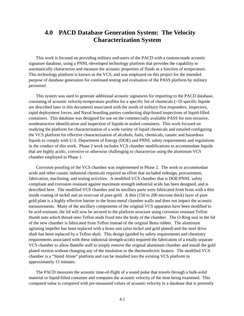
This work is focused on providing military end-users of the PACD with a custom-made acoustic signature database, using a PNNL-developed technology platform that provides the capability to automatically characterize and measure the acoustic properties of fluids as a function of temperature. This technology platform is known as the VCS, and was employed on this project for the intended purpose of database generation for continued testing and evaluation of the PASS platform by military personnel.
This system was used to generate additional acoustic signatures for importing to the PACD database, consisting of acoustic velocity-temperature profiles for a specific list of chemicals (~10 specific liquids are described later in this document) associated with the needs of military first responders, inspectors, rapid deployment forces, and Naval boarding parties conducting ship-board inspections of liquid-filled containers. This database was designed for use on the commercially available PASS for non-invasive, nondestructive identification and inspection of liquids in sealed containers. This work focused on readying the platform for characterization of a wide variety of liquid chemicals and entailed configuring the VCS platform for effective characterization of alcohols, fuels, chemicals, caustic and hazardous liquids to comply with U.S. Department of Energy (DOE) and PNNL safety requirements and regulations in the conduct of this work. Phase 2 work includes VCS chamber modifications to accommodate liquids that are highly acidic, corrosive or otherwise challenging to characterize using the aluminum VCS chamber employed in Phase 1.
Corrosion proofing of the VCS chamber was implemented in Phase 2. The work to accommodate acids and other caustic industrial chemicals required an effort that included redesign, procurement, fabrication, machining, and testing activities. A modified VCS chamber that is DOE/PNNL safety compliant and corrosion resistant against maximum strength industrial acids has been designed, and is described here. The modified VCS chamber and its ancillary parts were fabricated from brass with a thin inside coating of nickel and an overcoat of pure-gold. A thin (150 to 200 microns thick) layer of pure gold plate is a highly effective barrier to the brass-metal chamber walls and does not impact the acoustic measurements. Many of the ancillary components of the original VCS apparatus have been modified to be acid resistant; the lid will now be secured to the platform structure using corrosion resistant Teflon thumb nuts which thread onto Teflon studs fixed into the body of the chamber. The O-Ring seal in the lid of the new chamber is fabricated from Teflon instead of the original Buna rubber. The aluminum agitating impeller has been replaced with a brass unit (also nickel and gold plated) and the steel drive shaft has been replaced by a Teflon shaft. This design (guided by safety requirements and chemistry requirements associated with these industrial strength-acids) required the fabrication of a totally separate VCS chamber to allow Battelle staff to simply remove the original aluminum chamber and install the gold plated version without changing any of the insulation or the thermoelectric heaters. The modified VCS chamber is a “Stand Alone” platform and can be installed into the existing VCS platform in approximately 15 minutes.
The PACD measures the acoustic time-of-flight of a sound pulse that travels through a bulk-solid material or liquid-filled container and computes the acoustic velocity of the item being examined. This computed value is compared with pre-measured values of acoustic velocity in a database that is presently
4.2
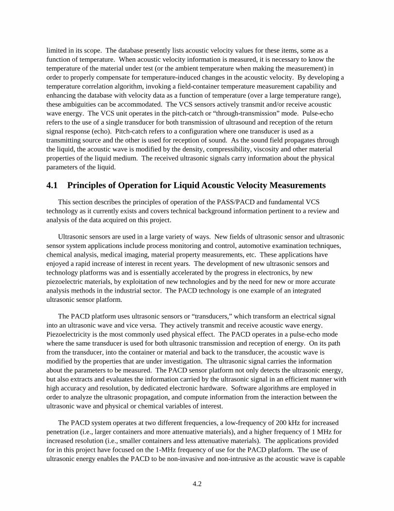
limited in its scope. The database presently lists acoustic velocity values for these items, some as a function of temperature. When acoustic velocity information is measured, it is necessary to know the temperature of the material under test (or the ambient temperature when making the measurement) in order to properly compensate for temperature-induced changes in the acoustic velocity. By developing a temperature correlation algorithm, invoking a field-container temperature measurement capability and enhancing the database with velocity data as a function of temperature (over a large temperature range), these ambiguities can be accommodated. The VCS sensors actively transmit and/or receive acoustic wave energy. The VCS unit operates in the pitch-catch or “through-transmission” mode. Pulse-echo refers to the use of a single transducer for both transmission of ultrasound and reception of the return signal response (echo). Pitch-catch refers to a configuration where one transducer is used as a transmitting source and the other is used for reception of sound. As the sound field propagates through the liquid, the acoustic wave is modified by the density, compressibility, viscosity and other material properties of the liquid medium. The received ultrasonic signals carry information about the physical parameters of the liquid.
4.1 Principles of Operation for Liquid Acoustic Velocity Measurements
This section describes the principles of operation of the PASS/PACD and fundamental VCS technology as it currently exists and covers technical background information pertinent to a review and analysis of the data acquired on this project.
Ultrasonic sensors are used in a large variety of ways. New fields of ultrasonic sensor and ultrasonic sensor system applications include process monitoring and control, automotive examination techniques, chemical analysis, medical imaging, material property measurements, etc. These applications have enjoyed a rapid increase of interest in recent years. The development of new ultrasonic sensors and technology platforms was and is essentially accelerated by the progress in electronics, by new piezoelectric materials, by exploitation of new technologies and by the need for new or more accurate analysis methods in the industrial sector. The PACD technology is one example of an integrated ultrasonic sensor platform.
The PACD platform uses ultrasonic sensors or “transducers,” which transform an electrical signal into an ultrasonic wave and vice versa. They actively transmit and receive acoustic wave energy. Piezoelectricity is the most commonly used physical effect. The PACD operates in a pulse-echo mode where the same transducer is used for both ultrasonic transmission and reception of energy. On its path from the transducer, into the container or material and back to the transducer, the acoustic wave is modified by the properties that are under investigation. The ultrasonic signal carries the information about the parameters to be measured. The PACD sensor platform not only detects the ultrasonic energy, but also extracts and evaluates the information carried by the ultrasonic signal in an efficient manner with high accuracy and resolution, by dedicated electronic hardware. Software algorithms are employed in order to analyze the ultrasonic propagation, and compute information from the interaction between the ultrasonic wave and physical or chemical variables of interest.
The PACD system operates at two different frequencies, a low-frequency of 200 kHz for increased penetration (i.e., larger containers and more attenuative materials), and a higher frequency of 1 MHz for increased resolution (i.e., smaller containers and less attenuative materials). The applications provided for in this project have focused on the 1-MHz frequency of use for the PACD platform. The use of ultrasonic energy enables the PACD to be non-invasive and non-intrusive as the acoustic wave is capable

4.3
of penetrating through bulk-solid commodities and through the walls of liquid-filled containers. The PACD is based on the use of compressional (or longitudinal) wave energy and generates the ultrasonic energy by utilizing piezoelectric materials. These two specific frequencies were chosen for providing optimal coverage and penetration while maintaining high sensitivity and resolution over a wide range of commodities, fluids and container sizes/geometries.
Acoustic velocity and attenuation are very valuable tools for the study of the physical properties of solids and liquids. These two very important parameters are defined by the solution
A = Ao e-αz cos(kz – ωt)
for an ultrasonic wave propagating in the z-direction with a propagation constant
k = 2π/λ = 2πf/ν
a radian frequency
ω = 2πf
and an attenuation coefficient α.
In these definitions, λ is the wavelength, f is the frequency, and ν is the phase velocity. In this traveling wave, the measurable quantities of interest to our application generally are ν and α. These two parameters are strongly dependent on the properties of the media the wave is traveling through, and both are the primary factors that determine the wave propagation. Molecular interactions, phase transitions, molecular rearrangements and other effects are responsible for the behavior of ν and α. The phase velocity is a function of the appropriate elastic modulus M of the mode being propagated; and the relationship is
ν = (M/ρ)1/2
where ρ is the density. For fluids the modulus M is the adiabatic bulk modulus B and the waves are longitudinal (which is the case for applications with the PACD). For solids, M is an appropriate combination of the elastic moduli of the solid itself and is influenced by many physical phenomena.
In an unbound solid medium, the compressional (longitudinal) velocity of sound is given as
νL2 = [K + (4/3)G] ρ-1
where K is the bulk modulus, G is the shear modulus, and ρ is the density. For fluid systems, the behavior of ultrasonic energy is more complicated in comparison to other materials. In liquids, the velocity of sound is described by
νL2 = (1/ρβ) = (B/ρ)
where β is the adiabatic compressibility of the fluid and B is the adiabatic bulk modulus. β, B and ρ are substance-specific integral parameters. In electrolytes, for instance, β changes very strongly with little
4.4
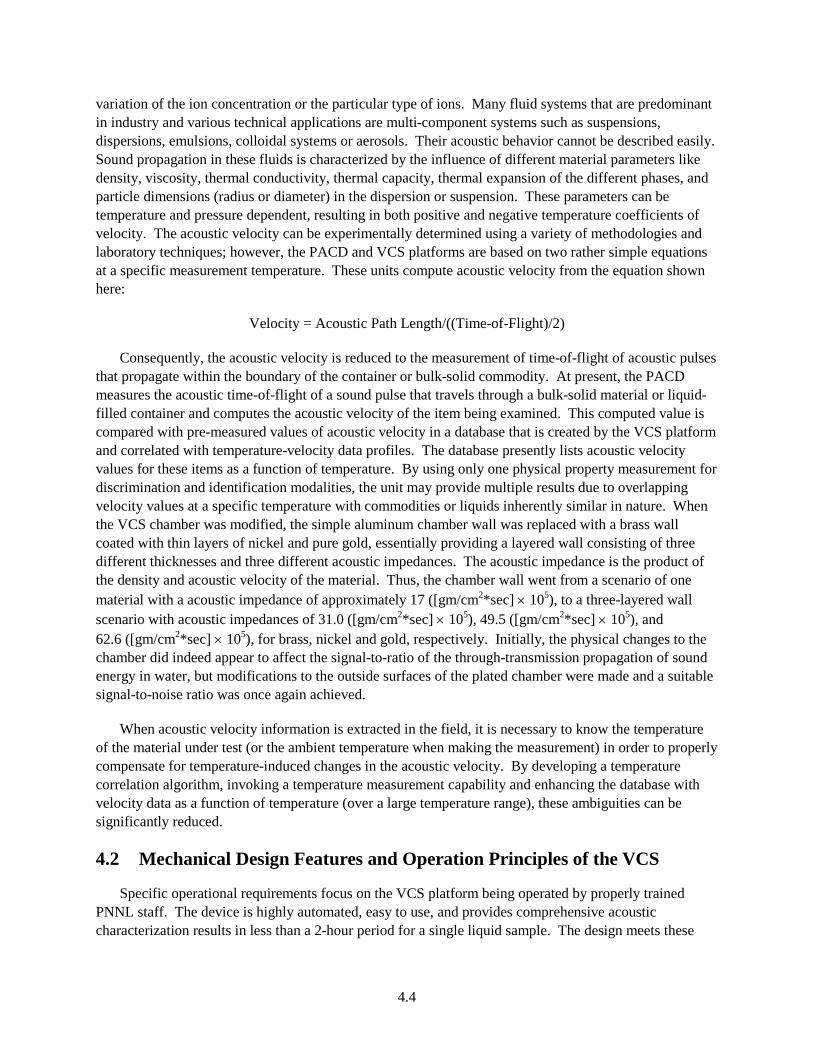
variation of the ion concentration or the particular type of ions. Many fluid systems that are predominant in industry and various technical applications are multi-component systems such as suspensions, dispersions, emulsions, colloidal systems or aerosols. Their acoustic behavior cannot be described easily. Sound propagation in these fluids is characterized by the influence of different material parameters like density, viscosity, thermal conductivity, thermal capacity, thermal expansion of the different phases, and particle dimensions (radius or diameter) in the dispersion or suspension. These parameters can be temperature and pressure dependent, resulting in both positive and negative temperature coefficients of velocity. The acoustic velocity can be experimentally determined using a variety of methodologies and laboratory techniques; however, the PACD and VCS platforms are based on two rather simple equations at a specific measurement temperature. These units compute acoustic velocity from the equation shown here:
Velocity = Acoustic Path Length/((Time-of-Flight)/2)
Consequently, the acoustic velocity is reduced to the measurement of time-of-flight of acoustic pulses that propagate within the boundary of the container or bulk-solid commodity. At present, the PACD measures the acoustic time-of-flight of a sound pulse that travels through a bulk-solid material or liquid-filled container and computes the acoustic velocity of the item being examined. This computed value is compared with pre-measured values of acoustic velocity in a database that is created by the VCS platform and correlated with temperature-velocity data profiles. The database presently lists acoustic velocity values for these items as a function of temperature. By using only one physical property measurement for discrimination and identification modalities, the unit may provide multiple results due to overlapping velocity values at a specific temperature with commodities or liquids inherently similar in nature. When the VCS chamber was modified, the simple aluminum chamber wall was replaced with a brass wall coated with thin layers of nickel and pure gold, essentially providing a layered wall consisting of three different thicknesses and three different acoustic impedances. The acoustic impedance is the product of the density and acoustic velocity of the material. Thus, the chamber wall went from a scenario of one material with a acoustic impedance of approximately 17 ([gm/cm2*sec] × 105), to a three-layered wall scenario with acoustic impedances of 31.0 ([gm/cm2*sec] × 105), 49.5 ([gm/cm2*sec] × 105), and 62.6 ([gm/cm2*sec] × 105), for brass, nickel and gold, respectively. Initially, the physical changes to the chamber did indeed appear to affect the signal-to-ratio of the through-transmission propagation of sound energy in water, but modifications to the outside surfaces of the plated chamber were made and a suitable signal-to-noise ratio was once again achieved.
When acoustic velocity information is extracted in the field, it is necessary to know the temperature of the material under test (or the ambient temperature when making the measurement) in order to properly compensate for temperature-induced changes in the acoustic velocity. By developing a temperature correlation algorithm, invoking a temperature measurement capability and enhancing the database with velocity data as a function of temperature (over a large temperature range), these ambiguities can be significantly reduced.
4.2 Mechanical Design Features and Operation Principles of the VCS
Specific operational requirements focus on the VCS platform being operated by properly trained PNNL staff. The device is highly automated, easy to use, and provides comprehensive acoustic characterization results in less than a 2-hour period for a single liquid sample. The design meets these

4.5
requirements and includes a heater/cooler platform using Peltier® devices; a data acquisition electronics module; high-frequency transducer (1 MHz); a system control module; a removable liquid containment module with retractable mixing device; and a laptop for data control, analysis and archival. Finally, specific portions of the system (where secondary containment is required) are placed within a berm for containment in the highly unlikely possibility of leaks during operation. Also, access to a suitably sized fume hood is required when characterizing hazardous fluids. The design includes consistently affixed ultrasonic transducers to the outer wall of the liquid containment module. The VCS is shown in Figure 4.1.
Figure 4.1. VCS System at PNNL Used for Database Generation for PASS
The ultrasonic velocity data are temperature-dependent physical properties of the propagation medium. The VCS platform collects, and passes to the laptop platform, digitized waveforms of the ultrasonic return signal along with the present temperature reading. On the laptop, a PNNL-developed algorithm uses this information, along with the path length measurement input, to accurately calculate a temperature-corrected ultrasonic velocity value. The technical details of the calculations are transparent to the user. Prior to characterization, the user inputs the required information, which may include temperature range, temperature increment step size, container information, etc. The characterization results are presented graphically for clear interpretation by the user at the end of the characterization run. The results are merged with the user input to form a separate report file that may be transmitted electronically, printed out on paper or archived for later retrieval. These calculated values are automatically ported to a database listing for the specific liquid being characterized and a comprehensive file for this liquid is generated and ready for downloading at the end of the characterization process. The data are plotted and a 2nd order polynomial fit is applied to the data. The equation of fit is then entered
4.6
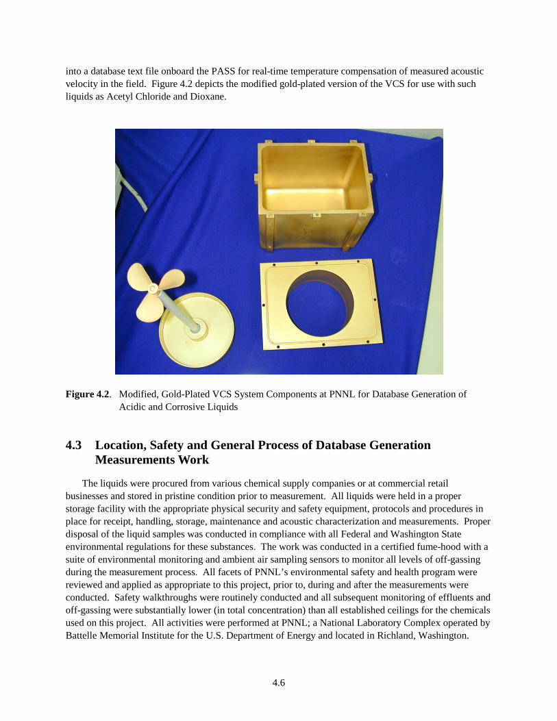
into a database text file onboard the PASS for real-time temperature compensation of measured acoustic velocity in the field. Figure 4.2 depicts the modified gold-plated version of the VCS for use with such liquids as Acetyl Chloride and Dioxane.
Figure 4.2. Modified, Gold-Plated VCS System Components at PNNL for Database Generation of
Acidic and Corrosive Liquids
4.3 Location, Safety and General Process of Database Generation Measurements Work
The liquids were procured from various chemical supply companies or at commercial retail businesses and stored in pristine condition prior to measurement. All liquids were held in a proper storage facility with the appropriate physical security and safety equipment, protocols and procedures in place for receipt, handling, storage, maintenance and acoustic characterization and measurements. Proper disposal of the liquid samples was conducted in compliance with all Federal and Washington State environmental regulations for these substances. The work was conducted in a certified fume-hood with a suite of environmental monitoring and ambient air sampling sensors to monitor all levels of off-gassing during the measurement process. All facets of PNNL’s environmental safety and health program were reviewed and applied as appropriate to this project, prior to, during and after the measurements were conducted. Safety walkthroughs were routinely conducted and all subsequent monitoring of effluents and off-gassing were substantially lower (in total concentration) than all established ceilings for the chemicals used on this project. All activities were performed at PNNL; a National Laboratory Complex operated by Battelle Memorial Institute for the U.S. Department of Energy and located in Richland, Washington.

5.1
5.0 Task 5 Results and Conclusions
5.1 Introduction to Dry Couplant Membrane Study
The PACD employs ultrasonic energy that originates at the face of a transducer requiring effective contact (referred to as acoustic “coupling”) to the surface of a liquid-filled container. The unit measures the time-of-flight of the propagating sound field that travels through the liquid and computes the acoustic velocity of the sound field from this measurement. The PACD algorithm compares the measured speed of sound to a database of acoustic velocity values, populated with several well characterized liquids, compensating for temperature variations and correlating the measured data point with the available data in the database. Thus, for optimum performance of the PACD, it is essential to have excellent coupling between the unit and the container in question in order to insert as much acoustic energy into the liquid medium as possible.
It has been known by the ultrasonic community (both industrial and medical realms) for decades that gels, such as ultrasonic gel couplant or common petroleum jelly, make excellent transduction layers for effective coupling of ultrasonic energy between transducers (sensors) and the objects being examined with ultrasound. Other liquid based materials such as water also aid in the coupling process between transducer and container. However, these wetting agents and coupling gels are typically messy, add additional steps to the measurement process, require the user to carry bottles of gel or wetting agents, and are generally undesirable to use in the field. Limitations include slowing down the efficiency of the user by requiring an unwanted step of applying a couplant enhancer in the measurement process. Gel couplants, in particular, leave behind a residue that is not desired by either the device user or container owner. The alternative to using couplant aided transducers is to find a transducer membrane that couples to a variety of containers with minimal ultrasonic signal loss. This type of coupling is known as dry-coupling.
Several variables must be taken into consideration when performing a dry couplant membrane study. In this study, it was determined that containers with flat sides are essential to ensure that all of the transducer face surface area was utilized, essentially eliminating surface curvature as a variable. A small diameter round container used in a laboratory environment would create non-coupled areas on either side of the transducer and allow for unwanted side-to-side shifting causing fluctuations in signal measure-ments. In field applications this tends not to be an issue since the container diameter tends to be much larger, simulating a flat surface. Simulating other field container properties, two distinctly different containers were selected for the study, each with unique ultrasonic properties; a steel container having greater acoustic impedance (~ 46 [gm/cm2*sec] × 105) with smooth sides and a high density poly ethylene (HDPE) container with minimal acoustic impedance (~ 1.7 [gm/cm2*sec] × 105) with typical rough sides. A membrane must perform well in both scenarios to be considered as a replacement to the current membrane.
The amount of pressure applied when coupling the transducer to the container wall must also be taken into careful consideration. Too much pressure will ultimately change the thickness of the membrane and potentially alter the container dimension thereby resulting in unwanted measurement variability. Too little pressure will not ensure proper coupling, thus causing the signal to fluctuate and may not allow for sufficient acoustic energy to propagate across the membrane layer into the contained liquid. After

5.2
multiple trials, the force of 23.8 Newtons was determined to be sufficient for an optimum coupling environment and used consistently for all membrane and baseline trials on the containers used in this study. Baseline trials were used to determine the experimental data boundaries in this dry coupling membrane study. Baselines were completed on all containers both with and without petroleum jelly couplant showing best- and worst-case coupling scenarios, respectively. This provided a data window that would ensure all further membrane trials would theoretically fall between these two data extremes.
5.2 Experimental Configuration and Pressure Calibration
The containers chosen for this project were rectangular in shape having dimensions 10 in. × 8 in. × 4 in. (where we used the 8-in. path length for sound propagation) for the steel container and 8 in. × 8 in. × 8 in. for the HDPE container. Each container was filled with water. The wall thickness for the steel container was 1/16 in. and the HDPE container wall thickness was measured at 1/8 in. The steel container had a painted smooth finish typical of steel drum containers, while the HDPE container has a rougher surface as found on most commercial HDPE containers. As previously mentioned these containers lie near opposite ends of the acoustic impedance spectrum with the exception of such metals like Platinum (~ 70 [gm/cm2*sec] × 105) and Tungsten (~ 101 [gm/cm2*sec] × 105). Steel is generally representative of the higher end of the acoustic impedance spectrum while the HDPE material has an acoustic impedance value more on the order of Teflon, plastics, Plexiglas and slightly higher than water which is approximately 1.48 [gm/cm2*sec] × 105. Thus, it is systematically more difficult to couple and transmit sound into and out of a steel container. Because the target of the PASS unit is for multiple container types, it is an objective to find a dry couplant membrane that works well on both types of materials. The laboratory bench-top data acquisition system is shown in Figure 5.1. In addition to the containers described here, the following equipment was also employed for this study:
1. One triple modality axis apparatus 2. “C” clamps and stabilization equipment 3. Two rectangular containers filled with room temperature water (steel and HDPE) 4. Two 1 MHz PASS transducers for through transmission testing 5. One strain gauge load cell 6. One digital oscilloscope 7. One signal generator/pulser 8. One signal receiver/amplifier
It was critical to stabilize, secure and semi-permanently affix the receiving transducer with optimum coupling to the side wall of the container directly opposite (and in alignment with) the position where the transmission transducer is coupled. This was achieved by applying a liberal amount of petroleum jelly to the center of the bare receiving transducer face, then subsequently applying a medium sized bead of five minute epoxy to the front edge of the transducer casting and attaching it to the predetermined wall of the container. The receive transducer was held in position for several minutes until the epoxy set, securing the receiving transducer to the container wall. This procedure eliminated any variations in transducer alignment between the receiving and transmitting transducers as well as ensuring optimal coupling and allowing the experiment to focus on the effects of only the membrane on coupling efficiency.
5.3
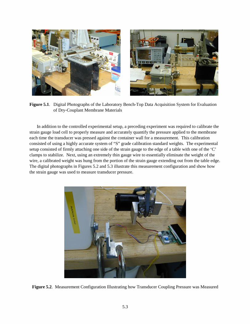
Figure 5.1. Digital Photographs of the Laboratory Bench-Top Data Acquisition System for Evaluation
of Dry-Couplant Membrane Materials
In addition to the controlled experimental setup, a preceding experiment was required to calibrate the strain gauge load cell to properly measure and accurately quantify the pressure applied to the membrane each time the transducer was pressed against the container wall for a measurement. This calibration consisted of using a highly accurate system of “S” grade calibration standard weights. The experimental setup consisted of firmly attaching one side of the strain gauge to the edge of a table with one of the ‘C’ clamps to stabilize. Next, using an extremely thin gauge wire to essentially eliminate the weight of the wire, a calibrated weight was hung from the portion of the strain gauge extending out from the table edge. The digital photographs in Figures 5.2 and 5.3 illustrate this measurement configuration and show how the strain gauge was used to measure transducer pressure.
Figure 5.2. Measurement Configuration Illustrating how Transducer Coupling Pressure was Measured

5.4
Figure 5.3. Digital Photographs Depicting the Calibration of the Strain Gauge Using a Set of NIST-
Calibrated Weights
The measurement procedures included recording the number from the digital display attached to the strain gauge for five individually weighted trials per weight, then compute the average. Table 5.1 shows the data from these calibration trials. Next, the average strain gauge display values vs. the calibration weights were plotted to extract the relationship between the true weight and the digital display weight. The plot in Figure 5.4 indicates a linear relationship, described by the equation Y = 0.0398x – 0.0387.
Table 5.1. Pressure Calibration Data for the Strain Gauge Used in This Study
Calibration Weight/Mass
(kg) Strain Gauge Display Average
0.5 14,14,14,14,14 14
1.0 26,26,26,26,26 26
2.0 51,51,51,51,51 51
3.0 76,76,76,76,76 76
5.0 127,127,127,127,127 127
Using this linear equation one can convert between the digital readout from the strain gauge display and the actual pressure applied from the transducer to the container wall.

5.5
Pressure Calibration (Strain Gauge Display vs. Standard Weights)
y = 0.0398x - 0.0387R2 = 0.9999
0.0
1.0
2.0
3.0
4.0
5.0
6.0
0 20 40 60 80 100 120 140
Strain Gauge Display
Stan
dard
Wei
ght (
kg)
Pressure Calibration Linear (Pressure Calibration)
Figure 5.4. Pressure Calibration Curve for the Strain Gauge Used to Compute Transducer Pressure
From the baseline measurements conducted at the onset of the trials, the amount of pressure on the transmitting transducer where the signal-to-noise was optimal was found to be at a reading of 62 on the strain gauge load cell. If more pressure was applied, the signal amplitude started to decrease and eventually signal shape became distorted due to pressure effects on the face of the transducer element. As pressure was reduced below this value, signal amplitude began to decrease, thus, the value of 62 was chosen for all trials for all membranes. At a reading of 62, this value corresponds to an applied mass of 2.4289 kg, which corresponds to an applied force of 23.8 Newtons. Throughout the trials, the pressure value on the strain gauge load cell was maintained to within a range of 61.0 to 62.0 (23.4 N to 23.8 N, respectively) essentially eliminating variability in transducer pressure between measurements.
5.3 Measurement Procedures
In considering apparatus alignment, it was imperative to accurately align the transmission transducer on the opposite container wall to that of the mounted receiving transducer. This is achieved by manipulating the triple axis manipulator (X-, Y-, Z-axes) with the attached transmission transducer into a position in which the full face of the transducer was in contact with the container wall and the signal received was maximized with regard to the peak-to-peak voltage. This ensured proper alignment in the X-Y plane corresponding to the two dimensions on the container wall, defaulting the Z-axis to control the pressure applied from the transducer to the wall (perpendicular to the wall).
Prior to data acquisition, it was necessary to position the strain gauge load cell into the zero pressure starting position. This was accomplished by maneuvering the transmitting transducer along the Z-axis into a position in which the full front face was just initiating contact with the container wall. Then placing the strain gauge load cell in contact with the ‘L’ bracket attached to the transducer and securely clamping the ‘L’ bracket holding the load cell to the table with the use of a ‘C’ clamp.
5.6
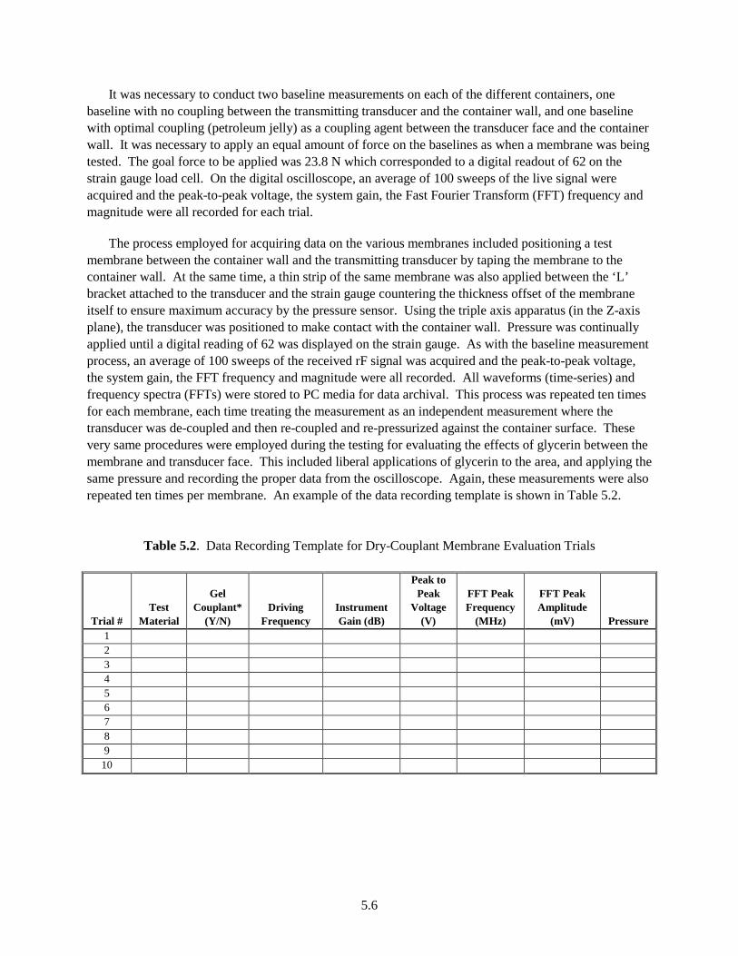
It was necessary to conduct two baseline measurements on each of the different containers, one baseline with no coupling between the transmitting transducer and the container wall, and one baseline with optimal coupling (petroleum jelly) as a coupling agent between the transducer face and the container wall. It was necessary to apply an equal amount of force on the baselines as when a membrane was being tested. The goal force to be applied was 23.8 N which corresponded to a digital readout of 62 on the strain gauge load cell. On the digital oscilloscope, an average of 100 sweeps of the live signal were acquired and the peak-to-peak voltage, the system gain, the Fast Fourier Transform (FFT) frequency and magnitude were all recorded for each trial.
The process employed for acquiring data on the various membranes included positioning a test membrane between the container wall and the transmitting transducer by taping the membrane to the container wall. At the same time, a thin strip of the same membrane was also applied between the ‘L’ bracket attached to the transducer and the strain gauge countering the thickness offset of the membrane itself to ensure maximum accuracy by the pressure sensor. Using the triple axis apparatus (in the Z-axis plane), the transducer was positioned to make contact with the container wall. Pressure was continually applied until a digital reading of 62 was displayed on the strain gauge. As with the baseline measurement process, an average of 100 sweeps of the received rF signal was acquired and the peak-to-peak voltage, the system gain, the FFT frequency and magnitude were all recorded. All waveforms (time-series) and frequency spectra (FFTs) were stored to PC media for data archival. This process was repeated ten times for each membrane, each time treating the measurement as an independent measurement where the transducer was de-coupled and then re-coupled and re-pressurized against the container surface. These very same procedures were employed during the testing for evaluating the effects of glycerin between the membrane and transducer face. This included liberal applications of glycerin to the area, and applying the same pressure and recording the proper data from the oscilloscope. Again, these measurements were also repeated ten times per membrane. An example of the data recording template is shown in Table 5.2.
Table 5.2. Data Recording Template for Dry-Couplant Membrane Evaluation Trials
Trial # Test
Material
Gel Couplant*
(Y/N) Driving
Frequency Instrument Gain (dB)
Peak to Peak
Voltage (V)
FFT Peak Frequency
(MHz)
FFT Peak Amplitude
(mV) Pressure 1 2 3 4 5 6 7 8 9
10

5.7
During this study, 11 different membrane materials were tested, and a total of 14 individual trials were conducted as some membrane samples consisted of various thicknesses. These membranes were tested with and without a wetting agent (glycerin) between the membrane and transducer face, thus requiring 28 total trials for each container. The entire set of measurements was conducted on both the steel and HDPE water-filled containers resulting in 56 total trials being conducted over the life of the study. Appendix A contains digital photographs of all the membrane materials evaluated and described here. Table 5.3 provides a listing of the materials evaluated here. Where information was not available or where the company would not reveal proprietary specifications for their membrane materials, the table is populated with “--”.
Table 5.3. Membrane Materials Evaluated in this Study
Company Material Thickness Density (kg/m3)
Acoustic Velocity
(m/s)
Loss @ 5 MHz
(dB/mm) Robustness Comments Olympus
NDT Aqualene 0.50 mm 920 1550-1600 0.28 Rigid
material Attracts dirt and
debris easily Olympus
NDT Aqualene 2.00 mm 920 1550-1600 0.28 Rigid
material --
Olympus NDT Aqualene 2.50 mm 920 1550-
1600 0.28 Rigid material --
Sigma Transducers DCMA 1:1 0.66 mm -- 1309 -- Rigid
material --
Sigma Transducers DCMA 1:2 0.61 mm -- 1239 -- Soft material --
Sigma Transducers
DCMB 1.25:2 1.09 mm -- 2204 -- Rigid
material --
Sigma Transducers DCMB 1:3 0.86 mm -- 1703 -- Soft material
Too soft, will not hold up in field
testing
Keener Rubber
Synthetic Polyisoprene 1.00 mm
SG 0.98-1.21
-- -- Rigid material
Rough surface, might cause problems on
some containers Standard
Commercial Black Rubber 0.80 mm -- -- -- Rigid material --
Standard Commercial Black Rubber 1.50 mm -- -- -- Rigid
material Too Rigid, does
not flex well Standard
Commercial Orange Rubber 0.80 mm -- -- -- Rigid
material --
Standard Commercial Red Gasket 1.64 mm -- -- -- Rigid
material Too Rigid, does
not flex well Standard
Commercial Vinyl Glove 0.15 mm -- -- -- Soft material --
Standard Commercial N-Dex Plus 0.16 mm -- -- -- Soft material --

5.8
Another critical parameter for consideration is the thickness of the membrane in relation to the wavelength of the sound field being propagated by the transducer. If the membrane is too thick, on the order of one-half the wavelength of the sound pulse generated from the transducer or higher harmonics, a standing wave can be constructed within the membrane material itself. This standing wave is a result of impedance mismatches between the membrane and the container wall causing no or very little sound energy to be transmitted into the container holding the liquid. Thus it is imperative that a membrane be chosen such that when pressure is brought to the membrane by pressing the transducer against the container, the actual thickness is not one-half the wavelength (or a harmonic thereof) of the pulse based on a driving frequency of 1 MHz.
V = f λ where: V = velocity of sound (m/s) f = frequency (Hz) λ = wavelength (m)
If we assume a membrane material with a sound speed close to that of water, say 1500 m/s, the wavelength at 1 MHz is 1.5 mm or about 0.06 inches. Therefore, some consideration should be made in choosing the thickness of the membrane to provide optimal thickness under contact pressure with the container wall and to provide optimal pliability and robustness for field applications.
5.4 Results
Throughout the experiment several key metrics were considered. First of several was the peak-to-peak amplitude of the radio frequency (rf) ultrasonic waveform (time series) displayed on the 100 sweep average of the digital oscilloscope. These data points revealed a clear picture as to which membranes were coupling well by showing just how much energy they transferred from the transducer into and through the container. The larger the peak-to-peak voltage, the more energy, and the closer the membrane was in comparison to the baseline (essentially optimal) coupling depicted by the Vaseline coupled baseline scenario described earlier.
A second, and equally important metric, was the frequency response of the sensor configuration using the FFT. An FFT was constructed using the 100 sweep average of the rf ultrasonic waveform (time series) on the oscilloscope to display the spectral response of the receiving transducer (essentially which frequency was highlighted as the most transmitted frequency). Due to the nature (bandwidth, nominal center frequency, excitation pulse, etc.) of the transducers employed on the PACD, while the transducer is nominally set to operate at a 1 MHz center frequency, several other frequencies are also produced in a bandwidth around 1 MHz. It is important to note which frequency is being received as the peak frequency (highest magnitude) since the optimal amount of acoustic energy being transmitted into the liquid media should occur near 1 MHz using the PACD. If this was not the case, and lower frequencies appeared to occur as the peak magnitudes in the spectrum, this would indicate that the membranes were responsible for “filtering” the higher frequencies and would present an undesirable effect.
Finally, the total system gain applied to the acoustic receive amplifier is an extremely important number to record for subsequent analysis and eventual comparison of data from individual measurement trials. Without knowledge of the proper gain setting between measurement trials, the recorded peak-to-peak voltage readings would be meaningless in a contrast to determine which membrane was the most

5.9
effective for this application. Once all the data was acquired, it was critical to normalize all the recorded data to a single ratio, at 0 dB gain. This placed all of the data collected from all the various membranes and containers on one level playing field enabling a direct comparison to be made. In order for a membrane to be considered as a replacement candidate it needed to perform well on both container types (steel and HDPE containers). Examples of rf ultrasonic signal responses and the corresponding frequency spectra for a membrane measurement are illustrated in Figures 5.5 and 5.6.
Aqualene (0.5mm) w/out GlycerinUltrasonic Waveform on Steel Container
-1.5
-1
-0.5
0
0.5
1
1.5
131 132 133 134 135 136 137
Time (µs)
Volta
ge (V
)
Figure 5.5. Example of the Recorded Ultrasonic Waveform (time-series) from the Digital Oscilloscope
for a Measurement Trial Using the 0.5-mm thick Aqualene Membrane without a Glycerin Wetting Agent Between the Transducer and the Membrane
Aqualene (0.5mm) w/out Glycerin Frequency Response (via FFT) on Steel Container
0
0.05
0.1
0.15
0.2
0.25
0.3
0.00 0.50 1.00 1.50 2.00 2.50 3.00 3.50 4.00
Frequency (MHz)
Volta
ge (m
V)
Figure 5.6. Example of the Frequency Spectrum (via an FFT) of the Time-Series in Figure 5.5
Depicting Frequency as a Function Magnitude

5.10
For a review of the summary tables showing the averaged data (normalized to 0 dB) and for individual waveforms and corresponding frequency spectra for all trials and both containers, please refer to Appendix B. The comparative representations illustrated in Figures 5.7, 5.8, and 5.9 show the primary bases for the recommendations provided in the next section.
Gain Normalized (to 0 dB) Peak-to-Peak Voltage on Steel Container (w/out a Gel Couplant Interface between Membrane and Transducer)
0
0.01
0.02
0.03
0.04
0.05
0.06
0.07
0.08
0.09
Baseli
ne
Curren
t Mem
brane
Aquale
ne (2
mm)
Aquale
ne (0
.5mm)
Polyiso
prene
Rub
ber
DCMA .026
1:1
DCMA .024
1:2
DCMB .043
1.25
:2
DCMB .034
1:3
Vinyl G
love
N-Dex
Plus
Black R
ubbe
r (1.5m
m)
Black R
ubbe
r (0.8m
m)
Orange
Rub
ber
Membrane
Volta
ge (V
)
Figure 5.7. Comparative Results for the Most Promising Membrane Materials as Applied to the Steel
Container without a Wetting Agent between the Membrane and the Transducer Face
Gain Normalized (to 0 dB) Peak-to-Peak Voltage on HDPE Container (w/out a Gel Couplant Interface between Membrane and Transducer)
0
1
2
3
4
5
6
7
8
Baseli
ne co
uplan
t
Baseli
ne no
coup
lant
Orange
Rub
ber
Black R
ubbe
r (0.8m
m)
Jerry
Red
Gas
ket
Aquale
ne (0
.5mm)
Origina
l mem
brane
DCMA .024
1:2
DCMA .026
1:1
DCMB .043
1.25
:2
Membrane
Volta
ge (V
)
Figure 5.8. Comparative Results for the Most Promising Membrane Materials as Applied to the HDPE
Container without a Wetting Agent between the Membrane and the Transducer Face

5.11
Gain Normalized (to 0 dB) Peak-to-Peak Voltage on Steel Container (with a Gel Couplant Interface between Membrane and Transducer)
0
0.01
0.02
0.03
0.04
0.05
0.06
0.07
0.08
Baseli
ne
Curren
t Mem
brane
Aquale
ne (2
.5mm)
Aquale
ne (2
mm)
Aquale
ne (0
.5mm)
Polyiso
prene R
ubbe
r
DCMA .026
1:1
DCMA .024
1:2
DCMB .043
1.25
:2
DCMB .034
1:3
Vinyl Glov
e
N-Dex
Plus
Black R
ubber
(1.5m
m)
Black R
ubber
(0.8m
m)
Orange R
ubbe
r
Membrane
Volta
ge (V
)
Figure 5.9. Comparative Results for the Most Promising Membrane Materials as Applied to the Steel
Container with a Wetting Agent between the Membrane and the Transducer Face
5.5 Conclusions and Recommendations
The current membrane in use on the PACD unit is a fairly effective material-couplant configuration for employing the PACD in the field. However, in some instances, signal amplitudes are marginal or non-existent without the addition of an additional mist of water or other wetting agent between the container wall and the membrane itself. This study was aimed at evaluating a wide range of potential material-membrane candidates for evaluation and comparison to the existing membrane configuration in order to identify a more effective membrane material for coupling acoustic energy into both plastic and steel containers using the PACD. The current membrane works well on the smooth surface of the steel container and competes with several other membranes for the top coupling material, however, when this membrane is employed for coupling to a rougher surface with a lower acoustic impedance than metals, it is easily out-performed by several other potential membranes such as the Sigma Transducer-made DCMA 1:2 soft membrane material.
Throughout the study it was determined that some materials (such as the DCMB 1:3 material) are on the extreme soft side, resulting in low longevity and life of a membrane that requires redundant field use in a MIO environment. Further, the extreme malleability of these membranes appears to alter the acoustic signal under different pressures and conditions. Although this type of material makes for a great coupling membrane for rough surfaces with the ability to squeeze into the microscopic surface crevices, it is not recommended as a potential membrane for applications where the PACD is required to operate. In a review of the trials conducted here, it became apparent that the requirement for a wetting agent (coupling liquid barrier) between the membrane and the transducer face was not required, and in some cases was actually detrimental to a suitable signal-to-noise. This additional layer of liquid (depending on the liquid barrier thickness) can reduce the amount of energy into the container rather than increase the coupling effectiveness. Thus, the conclusions discussed here will focus on recommending a membrane that is cast
5.12
directly onto the face of the transducer or one that is potentially adhered via a thin layer of Superglue or similar product.
Based upon the results plotted in Figures 5.7 through 5.9, it is apparent that there are a couple of potential alternatives toward addressing improvements to the current coupling membrane performance. If the PACD unit were to employ two separate (and interchangeable) 1 MHz transducers, where one would be used for metal containers and one would be used for plastic containers, then the data suggest the use of the orange rubber material for steel applications and the DCMA 1:2 material for HDPE container inspections. If however, the operational requirements allow for only one transducer with a membrane that is optimal for both steel and plastic containers, the choice would be to cast the transducers with either the DCMA 1:1 or DCMA 1:2 membrane materials.
The recommended approach depends upon the flexibility of the client and end-users to accommodate a dual transducer PACD or a single transducer PACD. The DCMA materials (both the 1:1 and the 1:2 castings) evaluated in this study are materials that are deemed robust and tested. Sigma Transducer’s (a company located in Washington state with decades of experience in ultrasonic transducer manufacturer) provided the samples of the DCMA castings and noted several key areas where these materials perform better than other commercially available dry-coupling membranes. These membranes performed significantly better than the current membrane based on the peak-to-peak voltages on the HDPE container and performed at the same level on the steel container. The coupling to the HDPE container was markedly better as the HDPE surface introduces the factor of surface roughness. The DCMA 1:2 material had over 4 times the peak-to-peak voltage amplitude of the current membrane when dry coupled to the HDPE container. Not only does this material have excellent acoustic coupling capabilities but it also has robustness to last use after use. Finally, the makers of this membrane offer the ability to custom cast the membrane of required thickness directly onto the face of the transducer, eliminating the need for a liquid-backed membrane and a threaded-cap housing mechanism, and ensuring optimum coupling between the transducer and the membrane.
Another issue resolved within this study is the common practice with the current membrane to have a layer of glycerin in-between the transducer face and the coupling membrane. Upon comparison with glycerin backed membranes to those without the coupling aid, results indicated little to no improvement on coupling to the steel container. This result leads one to believe that there is not a coupling issue between the transducer and the membrane but rather only between the membrane and the container wall. For continued development of the PACD platform, the next step is to obtain the client-based decision on which membrane approach to take:
• Two separate and interchangeable transducers with custom membranes for steel (orange rubber material) and HDPE (DCMA 1:2 material) respectively, or
• A single membrane that can be effectively employed on both steel and HDPE containers (either DCMA 1:1 or 1:2 materials)
The first option allows for the best possible coupling each time the PACD is employed, and provides the maximum amount of acoustic energy into the liquid medium. The second option eliminates the need to change out transducers for metallic and non-metallic container inspection scenarios but the compromise is not always achieving the maximum acoustic coupling possible.

6.1
6.0 Task 6 Results and Conclusions
6.1 Additional Acoustic Characterization of Liquids
After the Go/No-Go meeting at PNNL in early August 2007, discussions were initiated to determine the liquids slated for characterization in Phase 2. Telephone conversations and email discussions were conducted and various liquid suggestions were routed to all participating organizations for vetting and eventual determination of a final list of liquids for characterization and inclusion into the PACD database. The final Phase 2 liquids list is provided in Table 6.1.
Table 6.1. Final Phase 2 Liquid List for Addition to the PACD Database
Liquid
Isopropanol (91% Isopropyl Alcohol)
Mineral Oil
Methyl Ethyl Ketone
Dioxane
Chlorobenzene
Acetyl Chloride
Hydrogen Peroxide 30%
Hydrogen Peroxide 35%
Hydrogen Peroxide 50% Iraqi Light Crude Oil
Saudi Light Crude Oil
The decision and identifying process for the final list of liquids was based upon criteria such as the level of difficulty in acquiring specific liquids (time, cost, availability and level of effort), measurement system requirements and ramifications, and client guidance. The two light crude oil samples have not yet been received at PNNL at the time of the writing of this document, and therefore have not been included in the discussion here, and have yet to be characterized for inclusion in the PACD database.
PNNL initiated early analysis of each liquid on the list, including an environment, safety and health assessment of each liquid based on the individual liquid properties, rheology and data found in the MSDS documentation for each liquid. PNNL then embarked on obtaining 4- to 5-liter volumes of each specific liquid and began to baseline the operation and performance of the VCS platform with de-ionized water as the reference liquid. Operational and measurement safety procedures and processes were generated and approved, all MSDS documentation was obtained, and all peripheral equipment such as pumps and hoses

6.2
for VCS evacuation of liquids were also acquired. The team began generating a procedure for handling the propeller and evacuation of liquids and disposal of waste that eventually became the basis for the most recent modified VCS SOP. All primary and sub-components of the VCS were labeled and separated for movement into a fume hood. Digital photographs were taken and the system was brought up for full operation once again for the effort in Phase 2. Multiple runs on de-ionized water were performed between 40°F and 120°F in 10°F increments (both temperature directions, from low-to-high and high-to-low). The VCS system was validated by comparing (baselining) the results to that of water values provided from the literature. In the field of ultrasonics, de-ionized water is the most prevalent liquid characterized using acoustic property measurements, and thus water is an ideal liquid metric for validation of the system performance. All of the previous trials from Phase 1 (and more recent trials using the modified VCS chamber) have provided our team with a better understanding of the impact of evaporation during the measurement process, the measurement variation (resultant polynomial fits) between runs on the same fluid, and the impact of chemical interactions between various liquids and the aluminum and gold-plated containers.
6.2 Industrial Hygiene Monitoring Results of VCS Liquids
During Phase 1, evaporation and outgassing of the liquid samples during VCS analysis were reduced to insignificant levels by employing various seal materials that were placed inside the mixing propeller housing to seat the housing on top of the VCS containment. This essentially eliminated any evaporation effects and significantly reduced outgassing during operation inside the fume hood. After successful completion of Phase 1 characterizations, safety personnel at PNNL deemed the process (as conducted per standard operating procedures) safe, and thus no longer required the monitoring of outgassing on liquids characterized in Phase 2.
6.3 VCS Calibration and Baselining
Multiple characterization runs on each liquid were conducted using fresh batch samples, as acoustic property results from the VCS previously indicated that the heating process affected the properties of the liquid by contributing to the loss of volatiles and/or other unknown constituents in the liquids that changed the properties of the liquid over time as the samples were heated and measured. Thus, multiple runs were indeed conducted, but each run was initiated with a fresh sample of liquid and each run was started from the cold temperature extreme over the range of temperatures defined for each test. This process resulted in very consistent results from run-to-run using the VCS. The exact same process for calibration and baselining the VCS platform was employed in Phase 2 as in Phase 1. All calibration, baselining, precision and accuracy trials were recorded and matched very well with data from Phase 1. For the details of this process and the calibration data acquired, the reader is referred to the Phase 1 Technical Letter Report entitled, PHASE 1 Technical Letter Report – TS-00358: Portable Acoustic Contraband Detector, report number PNNL-16751. Figure 6.1 provides data acquired on two VCS runs on water in the modified gold-plated chamber, plotted against the “water standard” data used from 14 independent water trials and corrected using the Del Grosso and Mader literature values.(a) When these data were compared to previous runs on water in Phase 1 and recent water runs in conducted during Phase 2 in the aluminum chamber, the correlation was very good. From an acoustic perspective, the chamber distance was identical to the previous aluminum chamber distance indicating the high quality
(a) Del Grosso VA and CW Mader. 1972. “Speed of sound in pure water.” J Acoust Soc Am 52:1442-1446.

6.3
and precision of the machining and plating efforts to meet the specifications provided to both the machinists and the platers. Multiple characterization runs were conducted on water over the course of the Phase 2 effort and VCS performance characteristics and reliability/consistency were again evaluated and validated. Technical confidence in the resultant characterization data is very high, and the VCS platform was routinely benchmarked using calibration runs on water to verify continued operational performance and measurement consistency and reliability throughout the measurement process.
Water comparison
1400
1420
1440
1460
1480
1500
1520
1540
1560
0 20 40 60 80 100 120 140
Temperature (deg F)
Velo
city
(m/s
)
Manually Corrected water Run 1 gold chamber Run 2 gold chamber Figure 6.1. Comparison of Water Data from Trials in the Modified, Gold-Plated VCS Chamber to that
of the Phase 1 Water Curve Used for Distance Determination in the Aluminum VCS Chamber from Values Obtained from Del Grosso and Mader (1972)(a)
PNNL met the number of liquids required to meet this deliverable and completed full acoustic characterizations of nine liquids. These liquids included: Isopropyl alcohol 91%, mineral oil, methylethylketone, dioxane, chlorobenzene, acetyl chloride, hydrogen peroxide (30%), hydrogen peroxide (35%), and hydrogen peroxide (50%). A composite representation of all liquid profiles of acoustic velocity versus temperature is illustrated in Figure 6.2. The range spanning the various acoustic velocities for the nine liquids is quite broad, where acetyl chloride exhibits the slowest velocities over a range of 0.95 km/sec to 1.15 km/sec and conversely where hydrogen peroxide (50%) exhibits the fastest velocity of the group with a speed of 1.65 km/sec. Each individual liquid velocity-temperature profile is provided in Appendix C. It was interesting to note that the acoustic velocity values for Hydrogen Peroxide did not change with temperature for any of the three concentrations we evaluated in this study. The sound speed for these liquids was constant over the temperature range, however, the sound speed values do indeed allow one to discriminate between the various concentrations with measurable differences between 30, 35, and 50% concentrations.
(a) Del Grosso VA and CW Mader. 1972. “Speed of sound in pure water.” J Acoust Soc Am 52:1442-1446.

6.4
After the PACD database was completed, PNNL staff members generated a new in-lab validation test procedure using a PNNL-owned model-1 PASS device on a subset of liquids over low, medium and high temperatures in a variety of available containers where appropriate (due to safety procedures). The validation results are provided in Appendix D, where individual plots illustrate the measured data points superimposed over the VCS-generated velocity-temperature profile. A subset of six liquids was used for this portion of the study, and they include the entire list of liquids with the exception of the hydrogen peroxides. The same validation procedures were employed here in Phase 2 as were used in Phase 1.
Composite Plot of All Phase 2 Liquid Profiles
850
950
1050
1150
1250
1350
1450
1550
1650
1750
0 20 40 60 80 100 120 140
Temperature (deg F)
Aco
ustic
Vel
ocity
(m/s
Isopropanol (91% Isopropyl Alcohol) Mineral Oil Methyl Ethyl Ketone Dioxane Chlorobenzene Acetyl ChlorideHydrogen Peroxide (30%) Hydrogen Peroxide (35%) Hydrogen Peroxide (50%)
Figure 6.2. Composite Plot of all Phase 2 Liquids Illustrating Acoustic Velocity as a Function of
Temperature. Trendlines are not shown here but the 2nd order polynomial fits are included in Appendix C.
The data acquired during the in-lab validation effort showed that all measured data were within 2.5% of the database values as a function of temperature, and many fell within a 1% margin. Smaller containers were used for this study to reduce costs associated with acquisition, storage, use and disposal of large volumes of liquids (i.e., 55-gallon drums). As the path length decreases, the differences between PASS-measured values and database values will diverge. Differences in waveform shape will contribute to this type of difference between PASS-measured values and database values as well, particularly in smaller containers where the signal detection algorithm breaks down. Variations in the operator-measured temperature and distance are much more significant sources of error than the margins discussed here. The final 2nd order polynomial fits for each liquid (describing the relationship between the acoustic velocity and temperature as measured by the VCS) is provided in Table 6.2.

6.5
Table 6.2. Final Phase 2 Liquid List with the Associated 2nd Order Polynomial Fit for Each Acoustic Velocity-Temperature Profile
Liquid Second Order Polynomial Fit; where X = Temperature in °F R2 Value
Isopropanol (91% Isopropyl Alcohol) y = -0.0014x2 - 1.7774x + 1288.9 0.9998 Mineral Oil y = 0.0024x2 - 2.4836x + 1589.6 0.9991 Methyl Ethyl Ketone y = 0.0018x2 - 2.663x + 1391.3 0.9998 Dioxane y = -0.0024x2 - 1.9812x + 1507.6 0.9992 Chlorobenzene y = 0.0015x2 - 2.3422x + 1438 0.9999 Acetyl Chloride y = 0.0016x2 - 2.4315x + 1220.7 0.9998 Hydrogen Peroxide 30% y = 1551.0 N/A Hydrogen Peroxide 35% y = 1560.8 N/A Hydrogen Peroxide 50% y = 1630.0 N/A

6.6

7.1
7.0 Discussion and Recommendations
PNNL was originally tasked with providing 5 to 10 liquid constituents to the Phase 2 PACD database for this effort. The additional database now contains 9 new liquids with complete and validated acoustic velocity-temperature profiles. Once the crude oil samples are received from Bahrain, the additional liquids list will total 11 new liquids. Also, leveraging from work conducted for the Office of National Drug Control Policy in their mission to use the PASS technology for classifying and/or identifying precursor chemicals to the manufacture of methamphetamine, a long list of additional industrial chemicals, solvents and acids will be provided to the client for addition to the PACD database.
The VCS-generated data are both accurate and precise, and provide the necessary information onboard the PACD platform for a second round of operational testing and evaluation of liquid identification and classification efforts in sealed, liquid-filled containers.
Of the nine liquids characterized for this effort, only the hydrogen peroxide liquids were physically measured by other means, due to degassing of the liquids once they are poured into the VCS chamber and agitated with the mixing propeller. These sample liquids were measured in-situ, at various times when ambient temperatures or colder temperatures induced from refrigeration provided data over a suitable range. Data were recorded and the profiles were generated. Subsequent validation of these profiles in the field has been conducted numerous times with multiple operators (using both the PASS and more advanced ultrasonic measurement systems) providing a high level of confidence in these data. All other liquids were characterized using the VCS platform. Appendix C provides the complete listing of the nine characterized liquids along with the VCS derived 2nd order polynomial fit equation for the velocity-temperature data. These equations are copied to the database text file where the PACD decision algorithms can access the file each time a temperature is entered and measurement is obtained. In this way, all field measurements taken with the PACD unit can be compared to the profiles generated in Phases 1 and 2 of this project.
The results of this measurement exercise strongly demonstrate that by employing ultrasonic property measurements of acoustic velocity where the distance and temperature are suitably acquired, effective identification/discrimination/classification of liquids are possible. Data from ultrasonic velocity measurements as a function of temperature are presented, and analysis of these data indicates that accurate and consistent acoustic measurements were subsequently obtained for validation purposes using the PACD technology from the outside of the container, non-invasively and nondestructively.
Ultrasonic energy can easily penetrate single-walled containers and has demonstrated a wide applicability toward measurement of metal, glass, plastic, ceramic and other materials where the air content in the material is nonexistent. Since ultrasonic energy does not propagate across air, container configurations that include air gaps, insulation, or double-walls will preclude the travel of ultrasonic energy into the container liquid contents. However, most standard commercially available liquids (from industrial chemicals and solvents to petroleum-based liquids and fuels) are packaged in single-walled metal or plastic containers, providing ample opportunities to employ ultrasonic energy in the measurement and detection of contraband or hidden items, liquid explosives and their precursors, other weapons of mass destruction liquids and dual-use, co-mingled mixtures and liquid constituents.
7.2
From Phase 1, a review of the standard deviation and coefficient of variance statistics show that the VCS data and associated PASS data are well correlated and both reliable and consistent. It is evident that when interrogating smaller containers 12 in. in diameter and less, the accuracy of the time-of-flight measurements is reduced and the capability to identify liquids consistently in smaller containers will not be as effective as it would be with the same liquids in larger containers. Data to validate this was collected for water in larger 55-gallon drums at similar temperatures and plotted on the same VCS-generated curve for water in Phase 1. From the work conducted in Phase 1, it was shown that the PACD-measured data on larger containers will indeed converge toward the VCS-generated profile.
The above observation is due to the effects of container wall thickness (and associated time-of-flight delays) relative to the overall time-of-flight across the diameter of the container. As the ratio of overall container diameter to wall thickness becomes larger, the impact of the walls on the resultant PASS-measured velocities is less significant and the data begin to converge toward the line, which is essentially the true-state liquid velocity. Another factor lies in the algorithm’s ability to consistently and reliably identify and capture the correct echo in the rf ultrasonic waveforms as they become more tightly spaced in the time domain due to the shorter path lengths and ringing in the walls. Generally speaking, the PACD platform will excel when the path lengths are approximately 8 in. or larger and where the wall thicknesses are on the order of 1/8 in. to 1/16 in. As the path length becomes larger, the composite time-of-flight values are not as significantly impacted by wall delays, and the algorithm can accommodate wall thicknesses of ¼ in. and greater in many scenarios.
The variability in the VCS measurement system from run-to-run on the same liquid is extremely low and the relative accuracy of the data acquired with this system as referenced to water values is also quite good. Conversely, PACD field measurements are predicated upon many more variables that could substantially impact the resultant measurement. The container distance measurement must be accurately determined and the temperature of the liquid (via a container surface temperature measurement) should be obtained to within approximately ±3 to 4°F or the resultant velocity data may not be representative of the liquid inside the container. Thus, care must be taken to initiate PASS measurements with accurate inputs to the system, especially if the primary capability of this device is to be focused on identification (classification) of liquids, and particularly if the containers are 12 in. in diameter and smaller.
The modified VCS chamber operated to (and exceeded) the design specifications, and now provides PNNL with additional capabilities to properly and safely characterize highly concentrated acids and other caustic and volatile liquids that may be targeted in later phases of this project.

8.1
8.0 PNNL Management and Technical Points of Contact
Steve Martin – Product Line Manager Integrated Systems Solutions National Security Directorate Pacific Northwest National Laboratory 902 Battelle Blvd MSIN: K8-21 Richland, Washington 99352 Phone: 509-372-4086 Fax: 509-375-2484 Email: [email protected]
Technical Point of Contact: Principal Scientist and Project Manager Aaron Diaz – Senior Staff Scientist National Security Directorate Applied Physics and Materials Characterization Sciences Group Pacific Northwest National Laboratory 2400 Stevens Drive MSIN: K5-26 Richland, Washington 99352 Phone: 509-375-2606 Fax: 509-375-6497 Email: [email protected] Management and Administration Point of Contact: Todd Samuel – Certified Project Manager (PMP) and Technical Group Manager Energy & Environmental Technology Directorate Technology Planning and Deployment Group Pacific Northwest National Laboratory 902 Battelle Blvd MSIN: K6-05 Richland, Washington 99352 Phone: 509-375-6707 Fax: 509-372-4370 Email: [email protected]

8.2

Appendix A
Digital Photographs of Membrane Materials Evaluated in this Study
(Various thicknesses of the same material are not shown.)


A.1
Figure A.1. Digital Photograph of the Synthetic Polyisoprene Membrane Material Sample
Figure A.2. Digital Photograph of the 2.5-mm-thick Aqualene Membrane Material Sample

A.2
Figure A.3. Digital Photograph of the Presently Used Membrane Material Sample
Figure A.4. Digital Photograph of the DCMA 1:2 Membrane Material Sample

A.3
Figure A.5. Digital Photograph of the DCMA 1:1 Membrane Material Sample
Figure A.6. Digital Photograph of the DCMB 1:3 Membrane Material Sample
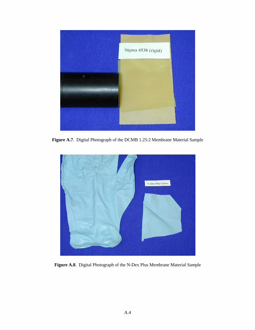
A.4
Figure A.7. Digital Photograph of the DCMB 1.25:2 Membrane Material Sample
Figure A.8. Digital Photograph of the N-Dex Plus Membrane Material Sample

A.5
Figure A.9. Digital Photograph of the Red Gasket Membrane Material Sample
Figure A.10. Digital Photograph of the Vinyl Glove Membrane Material Sample

A.6
Figure A.11. Digital Photograph of the Orange Rubber Membrane Material Sample
Figure A.12. Digital Photograph of the Thick Black Rubber Membrane Material Sample

Appendix B
Summary Tables and Representative rf Ultrasonic Waveforms and Frequency Spectra for all Membrane Trials


B.1
Table B.1. Summary of Averaged Membrane Measurements on Steel Container. All voltages were normalized to 0 dB (1:1 ratio).
Trial # Test Material
Gel Couplant**
(Y/N) Driving
Frequency Instrument Gain (dB)
Peak to Peak
Voltage (V)
Adj. Peak to Peak Voltage
(V)*
FFT Peak Frequency
(MHz)
FFT Peak Amplitude
(mV)
Adj.FFT Peak
Amplitude (mV)* Pressure
Pressure (N)
Avg Baseline Yes 1 MHz 28 1.831 0.07290 1.0000 234.2 9.32526 62 23.819372 Avg Baseline No 1 MHz 48 1.169 0.00466 1.2000 137.1 0.54588 62 23.819372 Avg Current Membrane No 1 MHz 32 1.816 0.04562 1.0000 259.3 6.51332 61 23.429068 Avg Current Membrane Yes 1 MHz 32 1.601 0.04022 1.0000 229.3 5.76001 61 23.429068 Avg Aqualene (2.5mm) Yes 1 MHz 32 1.829 0.04593 1.0000 260.6 6.54598 61 23.429068 Avg Aqualene (2 mm) No 1 MHz 31 1.723 0.04857 1.0800 229.5 6.46791 62 23.819372 Avg Aqualene (2 mm) Yes 1 MHz 31 1.772 0.04993 1.0000 246.5 6.94619 61.6 23.66325 Avg Aqualene (0.5mm) No 1 MHz 45.8 2.029 0.01041 1.0200 274.8 1.40924 61.3 23.546159 Avg Aqualene (0.5mm) Yes 1 MHz 37 1.852 0.02616 1.0200 242.2 3.42173 61.1 23.468098 Avg Polyisoprene Rubber No 1 MHz 40 1.407 0.01407 1.0000 211.6 2.11630 61.7 23.702281 Avg Polyisoprene Rubber Yes 1 MHz 38 1.732 0.02181 1.0400 220.1 2.77077 62 23.819372 Avg DCMA .026 1:1 No 1 MHz 32 1.848 0.04642 1.0000 282.6 7.09859 61.6 23.66325 Avg DCMA .026 1:1 Yes 1 MHz 32 1.845 0.04635 1.0000 278.9 7.00590 61.1 23.468098 Avg DCMA .024 1:2 No 1 MHz 32 1.642 0.04125 1.1000 250.2 6.28374 61 23.429068 Avg DCMA .024 1:2 Yes 1 MHz 32 1.719 0.04318 1.0000 257.3 6.46359 61 23.429068 Avg DCMB .043 1.25:2 No 1 MHz 30 1.861 0.05885 1.0000 258.5 8.17480 61.6 23.66325 Avg DCMB .043 1.25:2 Yes 1 MHz 30 1.709 0.05405 1.0000 241.2 7.62741 61.7 23.702281 Avg DCMB .034 1:3 No 1 MHz 30 1.606 0.05079 1.0000 243.2 7.69003 61 23.429068 Avg DCMB .034 1:3 Yes 1 MHz 30 1.647 0.05207 1.0000 238.2 7.53255 61.8 23.741311 Avg Vinyl Glove No 1 MHz 32 1.576 0.03959 1.2000 204.9 5.14761 61 23.429068 Avg Vinyl Glove Yes 1 MHz 32 1.734 0.04356 1.0200 233.9 5.87505 61 23.429068 Avg N-Dex Plus No 1 MHz 35.6 1.746 0.02898 1.2000 229.9 3.81556 61 23.429068 Avg N-Dex Plus Yes 1 MHz 36 1.664 0.02637 1.2000 212.5 3.36758 61 23.429068 Avg Black Rubber (1.5mm) No 1 MHz 28 1.606 0.06394 1.0000 227.7 9.06570 61 23.429068 Avg Black Rubber (1.5mm) Yes 1 MHz 28 1.325 0.05275 1.0000 189.0 7.52423 62 23.819372 Avg Black Rubber (0.8mm) No 1 MHz 28 1.586 0.06315 1.0000 233.8 9.30615 62 23.819372 Avg Black Rubber (0.8mm) Yes 1 MHz 28 0.979 0.03897 1.0000 137.8 5.48671 62 23.819372 Avg Orange Rubber No 1 MHz 28 1.954 0.07777 1.0000 291.1 11.58771 61.7 23.702281 Avg Orange Rubber Yes 1 MHz 28 1.621 0.06454 1.0000 232.6 9.25878 62 23.819372

B.2
Table B.2. Summary of Averaged Membrane Measurements on HDPE Container. All voltages were normalized to 0 dB (1:1 ratio).
Trial # Test Material
Gel Couplant**
(Y/N) Driving
Frequency Instrument Gain (dB)
Peak to Peak
Voltage (V)
Adj. Peak to Peak Voltage
(V)*
FFT Peak Frequency
(MHz)
FFT Peak Amplitude
(mV)
Adj.FFT Peak
Amplitude (mV)* Pressure Pressure (N)
Avg Baseline Yes 1 MHz -10 2.388 7.55025 1.100 378.6800 1197.49130 62.0 23.81937 Avg Baseline No 1 MHz 34 2.294 0.04577 0.600 476.5300 9.50802 62.0 23.81937 Avg Orange Rubber No 1 MHz 12 2.218 0.55704 1.100 339.7700 85.34637 62.0 23.81937 Avg Black Rubber (0.8mm) No 1 MHz 12 2.476 0.62194 1.100 459.0400 115.30563 62.0 23.81937 Avg Jerry Red Gasket No 1 MHz 12 2.280 0.57279 1.100 353.340 88.75500 62.0 23.81937 Avg Aqualene (0.5mm) No 1 MHz 18 1.804 0.22715 1.100 272.5300 34.30949 62.0 23.81937 Avg Original membrane No 1 MHz 8 2.236 0.89005 1.100 397.4700 158.23566 61.7 23.70228 Avg DCMA .024 1:2 No 1 MHz -5 2.302 4.09324 1.100 395.1100 702.61598 61.8 23.74131 Avg DCMA .026 1:1 No 1 MHz -5 1.659 2.94963 1.100 269.6400 479.49526 61.7 23.70228 Avg DCMB .043 1.25:2 No 1 MHz 9 2.073 0.73563 1.100 366.0500 129.87944 62.1 23.8584

B.3
Aqualene (2mm) w/out glycerin Waveform on Steel
-1.5
-1
-0.5
0
0.5
1
1.5
131 132 133 134 135 136 137 138
Time (µs)
Volta
ge (V
)
Figure B.1. Ultrasonic Waveform for Aqualene (2 mm) without Glycerin on Steel
Aqualene (2mm) w/ glycerin Waveform on Steel
-1
-0.5
0
0.5
1
1.5
131 132 133 134 135 136 137 138
Time (µs)
Volta
ge (V
)
Figure B.2. Ultrasonic Waveform for Aqualene (2 mm) with Glycerin on Steel

B.4
Aqualene (0.5mm) w/out glycerin Waveform on Steel
-1.5
-1
-0.5
0
0.5
1
1.5
131 132 133 134 135 136 137
Time (µs)
Volta
ge (V
)
Figure B.3. Ultrasonic Waveform for Aqualene (0.5 mm) without Glycerin on Steel
Aqualene (0.5mm) w/ glycerin Waveform on Steel
-1.5
-1
-0.5
0
0.5
1
1.5
131 132 133 134 135 136 137
Time (µs)
Volta
ge (V
)
Figure B.4. Ultrasonic Waveform for Aqualene (0.5 mm) with Glycerin on Steel

B.5
Polyisoprene Rubber w/out glycerin Waveform on Steel
-1.5
-1
-0.5
0
0.5
1
1.5
131 132 133 134 135 136 137
Time (µs)
Volta
ge (V
)
Figure B.5. Ultrasonic Waveform for Polyisoprene without Glycerin on Steel
Polyisoprene Rubber w/ glycerin Waveform on Steel
-1.5
-1
-0.5
0
0.5
1
1.5
131 132 133 134 135 136 137
Time (µs)
Volta
ge (V
)
Figure B.6. Ultrasonic Waveform for Polyisoprene with Glycerin on Steel

B.6
DCMB 1.25:2 w/out glycerin Waveform on Steel
-1
-0.5
0
0.5
1
1.5
131 132 133 134 135 136 137
Time (µs)
Volta
ge (V
)
Figure B.7. Ultrasonic Waveform for DCMB 1.25:2 without Glycerin on Steel
DCMB 1.25:2 w/ glycerin Waveform on Steel
-1
-0.5
0
0.5
1
1.5
131 132 133 134 135 136 137
Time (µs)
Volta
ge (V
)
Figure B.8. Ultrasonic Waveform for DCMB 1.25:2 with Glycerin on Steel

B.7
DCMB 1:3 w/out glycerin Waveform on Steel
-1
-0.5
0
0.5
1
1.5
131 132 133 134 135 136 137
Time (µs)
Volta
ge (V
)
Figure B.9. Ultrasonic Waveform for DCMB 1:3 without Glycerin on Steel
DCMB 1:3 w/ glycerin Waveform on Steel
-1
-0.5
0
0.5
1
1.5
131 132 133 134 135 136 137
Time (µs)
Volta
ge (V
)
Figure B.10. Ultrasonic Waveform for DCMB 1:3 with Glycerin on Steel

B.8
DCMA 1:1 w/out glycerin Waveform on Steel
-1.5
-1
-0.5
0
0.5
1
1.5
130 131 132 133 134 135 136 137
Time (µs)
Volta
ge (V
)
Figure B.11. Ultrasonic Waveform for DCMA 1:1 without Glycerin on Steel
DCMA 1:1 w/ glycerin Waveform on Steel
-1.5
-1
-0.5
0
0.5
1
1.5
130 131 132 133 134 135 136 137
Time (µs)
Volta
ge (V
)
Figure B.12. Ultrasonic Waveform for DCMA 1:1 with Glycerin on Steel
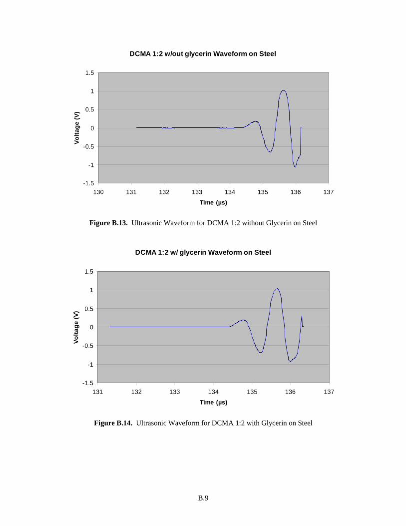
B.9
DCMA 1:2 w/out glycerin Waveform on Steel
-1.5
-1
-0.5
0
0.5
1
1.5
130 131 132 133 134 135 136 137
Time (µs)
Volta
ge (V
)
Figure B.13. Ultrasonic Waveform for DCMA 1:2 without Glycerin on Steel
DCMA 1:2 w/ glycerin Waveform on Steel
-1.5
-1
-0.5
0
0.5
1
1.5
131 132 133 134 135 136 137
Time (µs)
Volta
ge (V
)
Figure B.14. Ultrasonic Waveform for DCMA 1:2 with Glycerin on Steel

B.10
Current Membrane w/out glycerin Waveform on Steel
-1.5
-1
-0.5
0
0.5
1
1.5
131 132 133 134 135 136 137
Time (µs)
Volta
ge (V
)
Figure B.15. Ultrasonic Waveform for Current Membrane without Glycerin on Steel
Current Membrane w/ glycerin Waveform on Steel
-1.5
-1
-0.5
0
0.5
1
1.5
131 132 133 134 135 136 137
Time (µs)
Volta
ge (V
)
Figure B.16. Ultrasonic Waveform for Current Membrane with Glycerin on Steel

B.11
Vinyl glove w/out glycerin Waveform on Steel
-1.5
-1
-0.5
0
0.5
1
1.5
130 131 132 133 134 135 136 137
Time (µs)
Volta
ge (V
)
Figure B.17. Ultrasonic Waveform for Vinyl Glove Material without Glycerin on Steel
Vinyl glove w/ glycerin Waveform on Steel
-1
-0.5
0
0.5
1
1.5
130 131 132 133 134 135 136 137
Time (µs)
Volta
ge (V
)
Figure B.18. Ultrasonic Waveform for Vinyl Glove Material with Glycerin on Steel

B.12
N-Dex Plus w/out glycerin Waveform on Steel
-1.5
-1
-0.5
0
0.5
1
1.5
130 131 132 133 134 135 136 137
Time (µs)
Volta
ge (V
)
Figure B.19. Ultrasonic Waveform for N-Dex Plus Material without Glycerin on Steel
N-Dex Plus w/ glycerin Waveform on Steel
-1.5
-1
-0.5
0
0.5
1
1.5
130 131 132 133 134 135 136 137
Time (µs)
Volta
ge (V
)
Figure B.20. Ultrasonic Waveform for N-Dex Plus Material with Glycerin on Steel
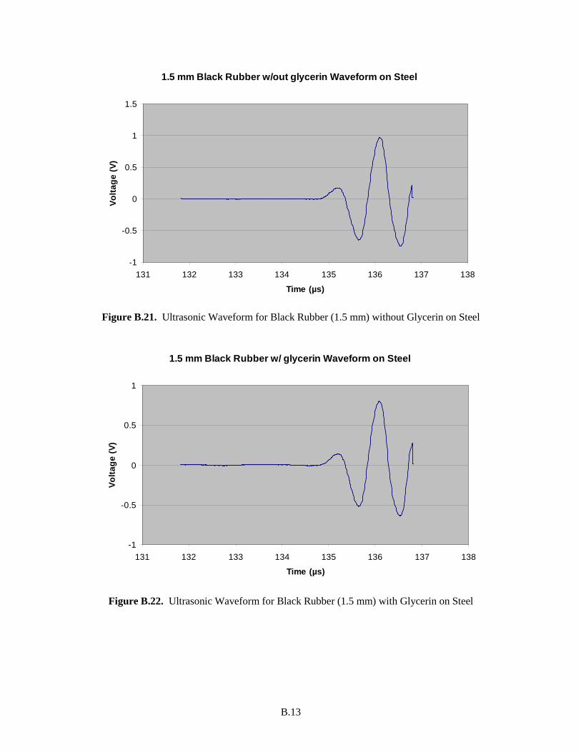
B.13
1.5 mm Black Rubber w/out glycerin Waveform on Steel
-1
-0.5
0
0.5
1
1.5
131 132 133 134 135 136 137 138
Time (µs)
Volta
ge (V
)
Figure B.21. Ultrasonic Waveform for Black Rubber (1.5 mm) without Glycerin on Steel
1.5 mm Black Rubber w/ glycerin Waveform on Steel
-1
-0.5
0
0.5
1
131 132 133 134 135 136 137 138
Time (µs)
Volta
ge (V
)
Figure B.22. Ultrasonic Waveform for Black Rubber (1.5 mm) with Glycerin on Steel

B.14
0.8 mm Black Rubber w/out glycerin Waveform on Steel
-1
-0.5
0
0.5
1
1.5
131 132 133 134 135 136 137
Time (µs)
Volta
ge (V
)
Figure B.23. Ultrasonic Waveform for Black Rubber (0.8 mm) without Glycerin on Steel
0.8 mm Black Rubber w/ glycerin Waveform on Steel
-1
-0.5
0
0.5
1
131 132 133 134 135 136 137
Time (µs)
Volta
ge (V
)
Figure B.24. Ultrasonic Waveform for Black Rubber (0.8 mm) with Glycerin on Steel

B.15
Orange Rubber w/out glycerin Waveform on Steel
-1.5
-1
-0.5
0
0.5
1
1.5
130 131 132 133 134 135 136 137
Time (µs)
Volta
ge (V
)
Figure B.25. Ultrasonic Waveform for Orange Rubber without Glycerin on Steel
Orange Rubber w/ glycerin Waveform on Steel
-1
-0.5
0
0.5
1
1.5
130 131 132 133 134 135 136 137
Time (µs)
Volta
ge (V
)
Figure B.26. Ultrasonic Waveform for Orange Rubber with Glycerin on Steel

B.16
Baseline w/out glycerin Waveform on Steel
-1
-0.5
0
0.5
1
130 131 132 133 134 135 136 137
Time (µs)
Volta
ge (V
)
Figure B.27. Ultrasonic Waveform for Baseline Measurement without Glycerin on Steel
Baseline w/ glycerin Waveform on Steel
-1
-0.5
0
0.5
1
1.5
130 131 132 133 134 135 136 137
Time (µs)
Volta
ge (V
)
Figure B.28. Ultrasonic Waveform for Baseline Measurement with Glycerin on Steel
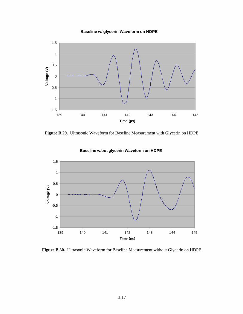
B.17
Baseline w/ glycerin Waveform on HDPE
-1.5
-1
-0.5
0
0.5
1
1.5
139 140 141 142 143 144 145
Time (µs)
Volta
ge (V
)
Figure B.29. Ultrasonic Waveform for Baseline Measurement with Glycerin on HDPE
Baseline w/out glycerin Waveform on HDPE
-1.5
-1
-0.5
0
0.5
1
1.5
139 140 141 142 143 144 145
Time (µs)
Volta
ge (V
)
Figure B.30. Ultrasonic Waveform for Baseline Measurement without Glycerin on HDPE
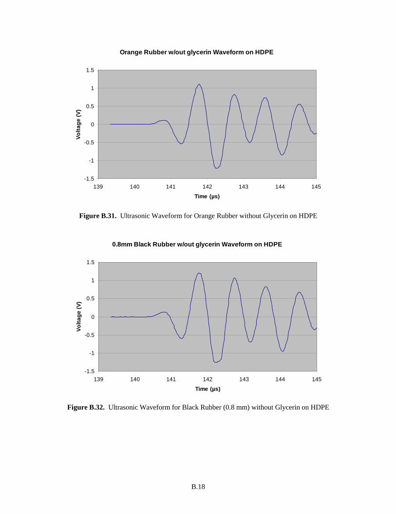
B.18
Orange Rubber w/out glycerin Waveform on HDPE
-1.5
-1
-0.5
0
0.5
1
1.5
139 140 141 142 143 144 145
Time (µs)
Volta
ge (V
)
Figure B.31. Ultrasonic Waveform for Orange Rubber without Glycerin on HDPE
0.8mm Black Rubber w/out glycerin Waveform on HDPE
-1.5
-1
-0.5
0
0.5
1
1.5
139 140 141 142 143 144 145
Time (µs)
Volta
ge (V
)
Figure B.32. Ultrasonic Waveform for Black Rubber (0.8 mm) without Glycerin on HDPE

B.19
Red Gasket w/out glycerin Waveform on HDPE
-1.5
-1
-0.5
0
0.5
1
1.5
140.5 141 141.5 142 142.5 143 143.5 144 144.5 145
Time (µs)
Volta
ge (V
)
Figure B.33. Ultrasonic Waveform for Red Gasket material without Glycerin on HDPE
Aqualene (0.5 mm) w/out glycerin Waveform on HDPE
-1
-0.5
0
0.5
1
139 140 141 142 143 144 145
Time (µs)
Volta
ge (V
)
Figure B.34. Ultrasonic Waveform for Aqualene (0.5 mm) without Glycerin on HDPE

B.20
Original Membrane w/out glycerin Waveform on HDPE
-1.5
-1
-0.5
0
0.5
1
1.5
139 140 141 142 143 144 145
Time (µs)
Volta
ge (V
)
Figure B.35. Ultrasonic Waveform for Current Membrane without Glycerin on HDPE
DCMA 1:2 w/out glycerin Waveform on HDPE
-1.5
-1
-0.5
0
0.5
1
1.5
139 140 141 142 143 144 145
Time (µs)
Volta
ge (V
)
Figure B.36. Ultrasonic Waveform for DCMA 1:2 without Glycerin on HDPE

B.21
DCMA 1:1 w/out glycerin Waveform on HDPE
-1
-0.5
0
0.5
1
139 140 141 142 143 144 145
Time (µs)
Volta
ge (V
)
Figure B.37. Ultrasonic Waveform for DCMA 1:1 without Glycerin on HDPE
DCMB 1.25:2 w/out glycerin Waveform on HDPE
-1.5
-1
-0.5
0
0.5
1
1.5
139 140 141 142 143 144 145
Time (µs)
Volta
ge (V
)
Figure B.38. Ultrasonic Waveform for DCMB 1.25:2 without Glycerin on HDPE

B.22
Aqualene (2mm) w/out glycerin FFT on Steel
0
0.05
0.1
0.15
0.2
0.25
0.3
0.00 0.50 1.00 1.50 2.00 2.50 3.00 3.50 4.00
Frequency (MHz)
Volta
ge (m
V)
Figure B.39. Frequency Spectrum for Aqualene (2 mm) without Glycerin on Steel
Aqualene (2mm) w/ glycerin FFT on Steel
0
0.05
0.1
0.15
0.2
0.25
0.3
0.00 0.50 1.00 1.50 2.00 2.50 3.00 3.50 4.00
Frequency (MHz)
Volta
ge (m
V)
Figure B.40. Frequency Spectrum for Aqualene (2 mm) with Glycerin on Steel
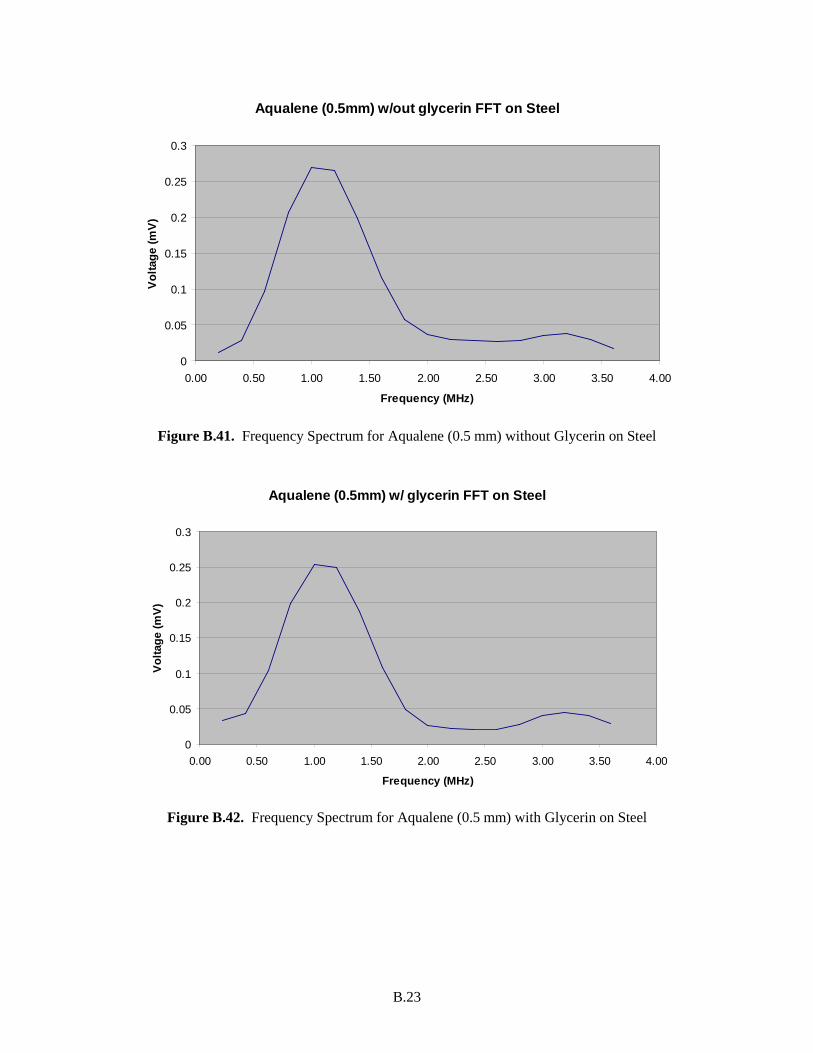
B.23
Aqualene (0.5mm) w/out glycerin FFT on Steel
0
0.05
0.1
0.15
0.2
0.25
0.3
0.00 0.50 1.00 1.50 2.00 2.50 3.00 3.50 4.00
Frequency (MHz)
Volta
ge (m
V)
Figure B.41. Frequency Spectrum for Aqualene (0.5 mm) without Glycerin on Steel
Aqualene (0.5mm) w/ glycerin FFT on Steel
0
0.05
0.1
0.15
0.2
0.25
0.3
0.00 0.50 1.00 1.50 2.00 2.50 3.00 3.50 4.00
Frequency (MHz)
Volta
ge (m
V)
Figure B.42. Frequency Spectrum for Aqualene (0.5 mm) with Glycerin on Steel

B.24
Polyisoprene Rubber w/out glycerin Waveform on Steel
0
0.05
0.1
0.15
0.2
0.25
0.3
0.35
0.00 0.50 1.00 1.50 2.00 2.50 3.00 3.50 4.00
Frequency (MHz)
Volta
ge (m
V)
Figure B.43. Frequency Spectrum for Polyisoprene Rubber without Glycerin on Steel
Polyisoprene Rubber w/ glycerin Waveform on Steel
0
0.05
0.1
0.15
0.2
0.25
0.3
0.00 0.50 1.00 1.50 2.00 2.50 3.00 3.50 4.00
Frequency (MHz)
Volta
ge (m
V)
Figure B.44. Frequency Spectrum for Polyisoprene Rubber with Glycerin on Steel
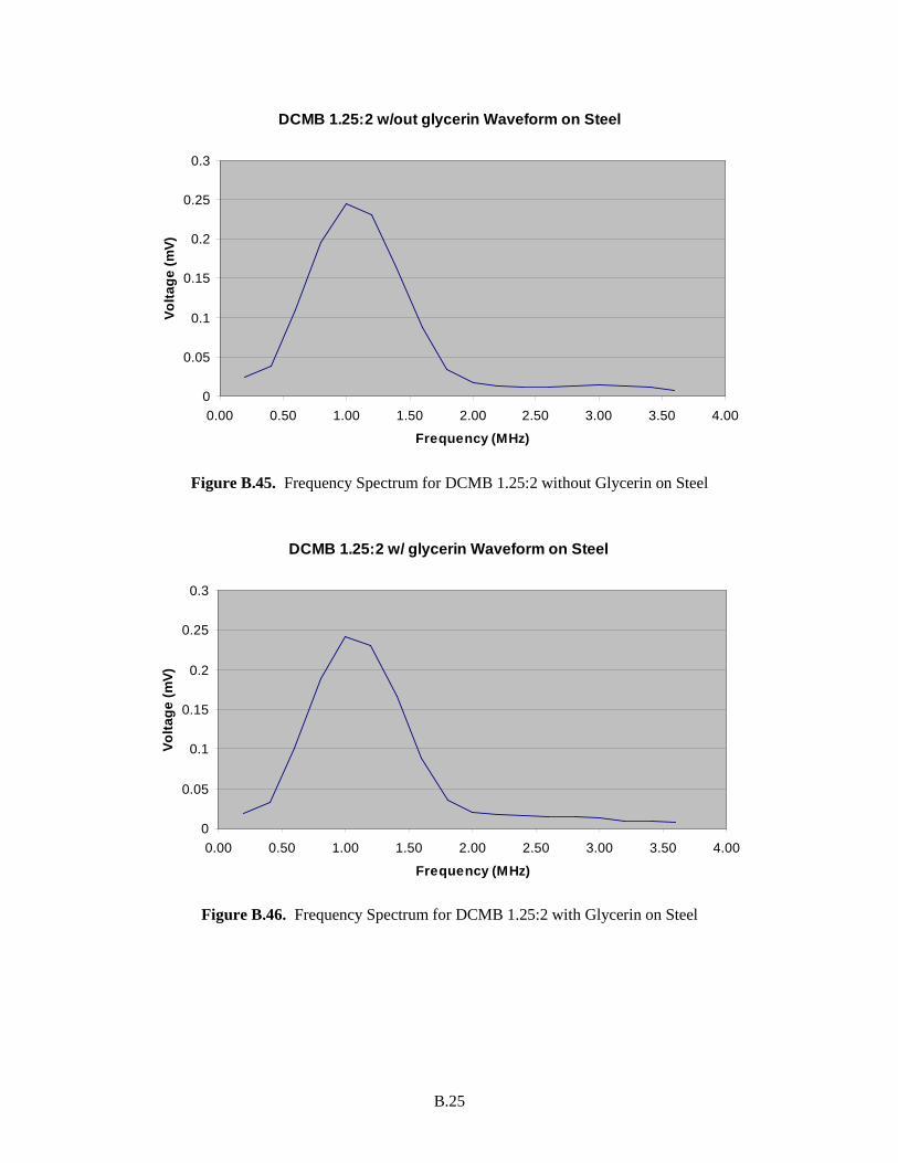
B.25
DCMB 1.25:2 w/out glycerin Waveform on Steel
0
0.05
0.1
0.15
0.2
0.25
0.3
0.00 0.50 1.00 1.50 2.00 2.50 3.00 3.50 4.00
Frequency (MHz)
Volta
ge (m
V)
Figure B.45. Frequency Spectrum for DCMB 1.25:2 without Glycerin on Steel
DCMB 1.25:2 w/ glycerin Waveform on Steel
0
0.05
0.1
0.15
0.2
0.25
0.3
0.00 0.50 1.00 1.50 2.00 2.50 3.00 3.50 4.00
Frequency (MHz)
Volta
ge (m
V)
Figure B.46. Frequency Spectrum for DCMB 1.25:2 with Glycerin on Steel

B.26
DCMB 1:3 w/out glycerin Waveform on Steel
0
0.05
0.1
0.15
0.2
0.25
0.3
0.00 0.50 1.00 1.50 2.00 2.50 3.00 3.50 4.00
Frequency (MHz)
Volta
ge (m
V)
Figure B.47. Frequency Spectrum for DCMB 1:3 without Glycerin on Steel
DCMB 1:3 w/ glycerin Waveform on Steel
0
0.05
0.1
0.15
0.2
0.25
0.00 0.50 1.00 1.50 2.00 2.50 3.00 3.50 4.00
Frequency (MHz)
Volta
ge (m
V)
Figure B.48. Frequency Spectrum for DCMB 1:3 with Glycerin on Steel

B.27
DCMA 1:1 w/out glycerin Waveform on Steel
0
0.05
0.1
0.15
0.2
0.25
0.3
0.00 0.50 1.00 1.50 2.00 2.50 3.00 3.50 4.00
Frequency (MHz)
Volta
ge (m
V)
Figure B.49. Frequency Spectrum for DCMA 1:1 without Glycerin on Steel
DCMA 1:1 w/ glycerin Waveform on Steel
0
0.05
0.1
0.15
0.2
0.25
0.3
0.00 0.50 1.00 1.50 2.00 2.50 3.00 3.50 4.00
Frequency (MHz)
Volta
ge (m
V)
Figure B.50. Frequency Spectrum for DCMA 1:1 with Glycerin on Steel
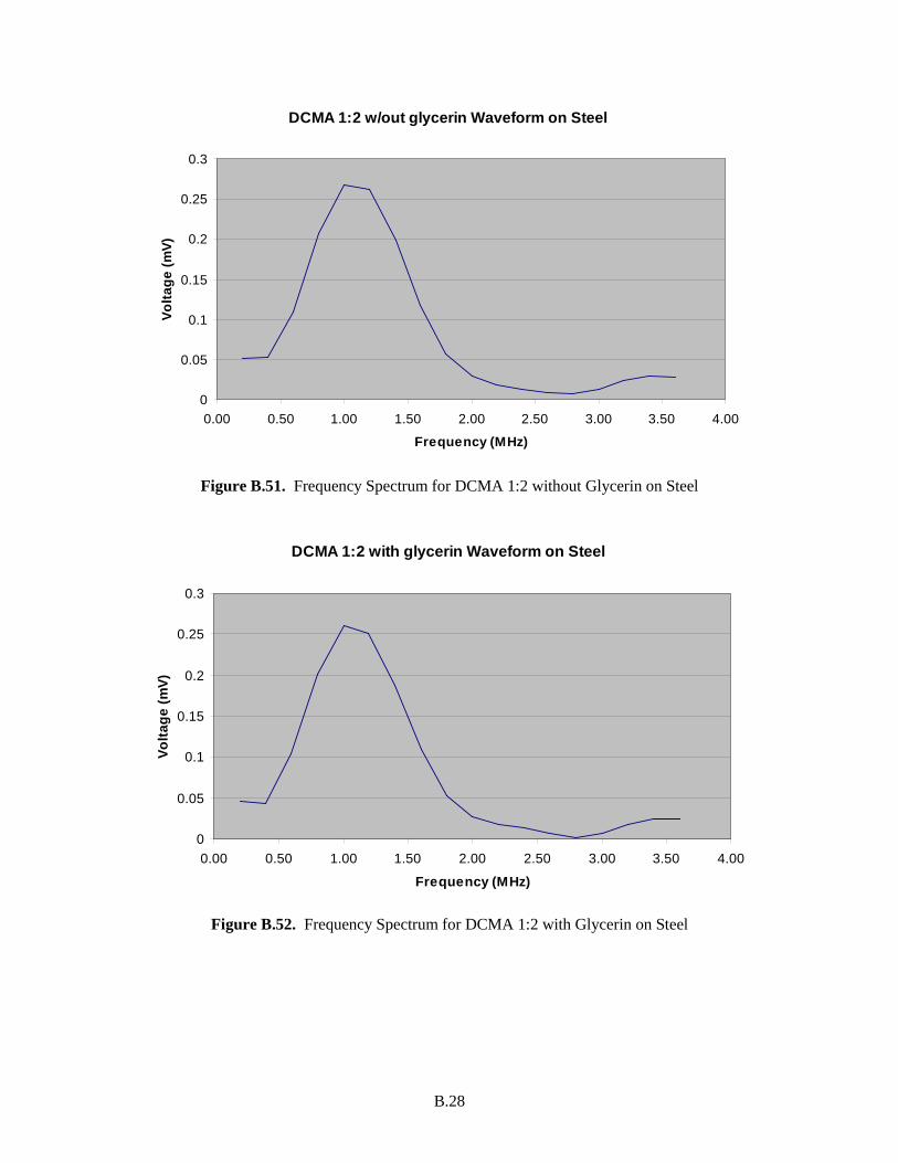
B.28
DCMA 1:2 w/out glycerin Waveform on Steel
0
0.05
0.1
0.15
0.2
0.25
0.3
0.00 0.50 1.00 1.50 2.00 2.50 3.00 3.50 4.00
Frequency (MHz)
Volta
ge (m
V)
Figure B.51. Frequency Spectrum for DCMA 1:2 without Glycerin on Steel
DCMA 1:2 with glycerin Waveform on Steel
0
0.05
0.1
0.15
0.2
0.25
0.3
0.00 0.50 1.00 1.50 2.00 2.50 3.00 3.50 4.00
Frequency (MHz)
Volta
ge (m
V)
Figure B.52. Frequency Spectrum for DCMA 1:2 with Glycerin on Steel

B.29
Current Membrane w/out glycerin Waveform on Steel
0
0.05
0.1
0.15
0.2
0.25
0.3
0.00 0.50 1.00 1.50 2.00 2.50 3.00 3.50 4.00
Frequency (MHz)
Volta
ge (m
V)
Figure B.53. Frequency Spectrum for Current Membrane Material without Glycerin on Steel
Current Membrane w/ glycerin Waveform on Steel
0
0.05
0.1
0.15
0.2
0.25
0.3
0.00 0.50 1.00 1.50 2.00 2.50 3.00 3.50 4.00
Frequency (MHz)
Volta
ge (m
V)
Figure B.54. Frequency Spectrum for Current Membrane Material with Glycerin on Steel

B.30
Vinyl Glove w/out glycerin Waveform on Steel
0
0.05
0.1
0.15
0.2
0.25
0.00 0.50 1.00 1.50 2.00 2.50 3.00 3.50 4.00
Frequency (MHz)
Volta
ge (m
V)
Figure B.55. Frequency Spectrum for Vinyl Glove Material without Glycerin on Steel
Vinyl Glove w/ glycerin Waveform on Steel
0
0.05
0.1
0.15
0.2
0.25
0.3
0.00 0.50 1.00 1.50 2.00 2.50 3.00 3.50 4.00
Frequency (MHz)
Volta
ge (m
V)
Figure B.56. Frequency Spectrum for Vinyl Glove Material with Glycerin on Steel

B.31
N-Dex Plus w/out glycerin Waveform on Steel
0
0.05
0.1
0.15
0.2
0.25
0.00 0.50 1.00 1.50 2.00 2.50 3.00 3.50 4.00
Frequency (MHz)
Volta
ge (m
V)
Figure B.57. Frequency Spectrum for N-Dex Plus Material without Glycerin on Steel
N-Dex Plus w/ glycerin Waveform on Steel
0
0.05
0.1
0.15
0.2
0.25
0.00 0.50 1.00 1.50 2.00 2.50 3.00 3.50 4.00
Frequency (MHz)
Volta
ge (m
V)
Figure B.58. Frequency Spectrum for N-Dex Plus Material with Glycerin on Steel

B.32
1.5 mm Black Rubber w/out glycerin Waveform on Steel
0
0.05
0.1
0.15
0.2
0.25
0.00 0.50 1.00 1.50 2.00 2.50 3.00 3.50 4.00
Frequency (MHz)
Volta
ge (m
V)
Figure B.59. Frequency Spectrum for Black Rubber (1.5 mm) without Glycerin on Steel
1.5 mm Black Rubber w/ glycerin Waveform on Steel
0
0.02
0.04
0.06
0.08
0.1
0.12
0.14
0.16
0.18
0.2
0.00 0.50 1.00 1.50 2.00 2.50 3.00 3.50 4.00
Frequency (MHz)
Volta
ge (m
V)
Figure B.60. Frequency Spectrum for Black Rubber (1.5 mm) with Glycerin on Steel

B.33
0.8 mm Black Rubber w/out glycerin Waveform on Steel
0
0.05
0.1
0.15
0.2
0.25
0.00 0.50 1.00 1.50 2.00 2.50 3.00 3.50 4.00
Frequency (MHz)
Volta
ge (m
V)
Figure B.61. Frequency Spectrum for Black Rubber (0.8 mm) without Glycerin on Steel
0.8 mm Black Rubber w/ glycerin Waveform on Steel
0
0.02
0.04
0.06
0.08
0.1
0.12
0.14
0.16
0.00 0.50 1.00 1.50 2.00 2.50 3.00 3.50 4.00
Frequency (MHz)
Volta
ge (m
V)
Figure B.62. Frequency Spectrum for Black Rubber (0.8 mm) with Glycerin on Steel

B.34
Orange Rubber w/out glycerin Waveform on Steel
0
0.05
0.1
0.15
0.2
0.25
0.3
0.35
0.00 0.50 1.00 1.50 2.00 2.50 3.00 3.50 4.00
Frequency (MHz)
Volta
ge (m
V)
Figure B.63. Frequency Spectrum for Orange Rubber without Glycerin on Steel
Baseline w/out glycerin Waveform on Steel
0
0.02
0.04
0.06
0.08
0.1
0.12
0.14
0.00 0.50 1.00 1.50 2.00 2.50 3.00 3.50 4.00
Frequency (MHz)
Volta
ge (m
V)
Figure B.64. Frequency Spectrum for Baseline Measurement without Glycerin on Steel

B.35
Baseline w/ glycerin Waveform on Steel
0
0.05
0.1
0.15
0.2
0.25
0.00 0.50 1.00 1.50 2.00 2.50 3.00 3.50 4.00
Frequency (MHz)
Volta
ge (m
V)
Figure B.65. Frequency Spectrum for Baseline Measurement with Glycerin on Steel
Baseline w/ glycerin Waveform on HDPE
0
0.05
0.1
0.15
0.2
0.25
0.3
0.35
0.4
0.45
0.00 0.50 1.00 1.50 2.00 2.50 3.00 3.50
Frequency (MHz)
Volta
ge (m
V)
Figure B.66. Frequency Spectrum for Baseline Measurement with Glycerin on HDPE

B.36
Baseline w/out glycerin Waveform on HDPE
0
0.05
0.1
0.15
0.2
0.25
0.3
0.35
0.4
0.45
0.5
0.00 0.50 1.00 1.50 2.00 2.50 3.00 3.50
Frequency (MHz)
Volta
ge (m
V)
Figure B.67. Frequency Spectrum for Baseline Measurement without Glycerin on HDPE
Orange Rubber w/out glycerin Waveform on HDPE
0
0.05
0.1
0.15
0.2
0.25
0.3
0.35
0.4
0.00 0.50 1.00 1.50 2.00 2.50 3.00 3.50
Frequency (MHz)
Volta
ge (m
V)
Figure B.68. Frequency Spectrum for Orange Rubber Material without Glycerin on HDPE
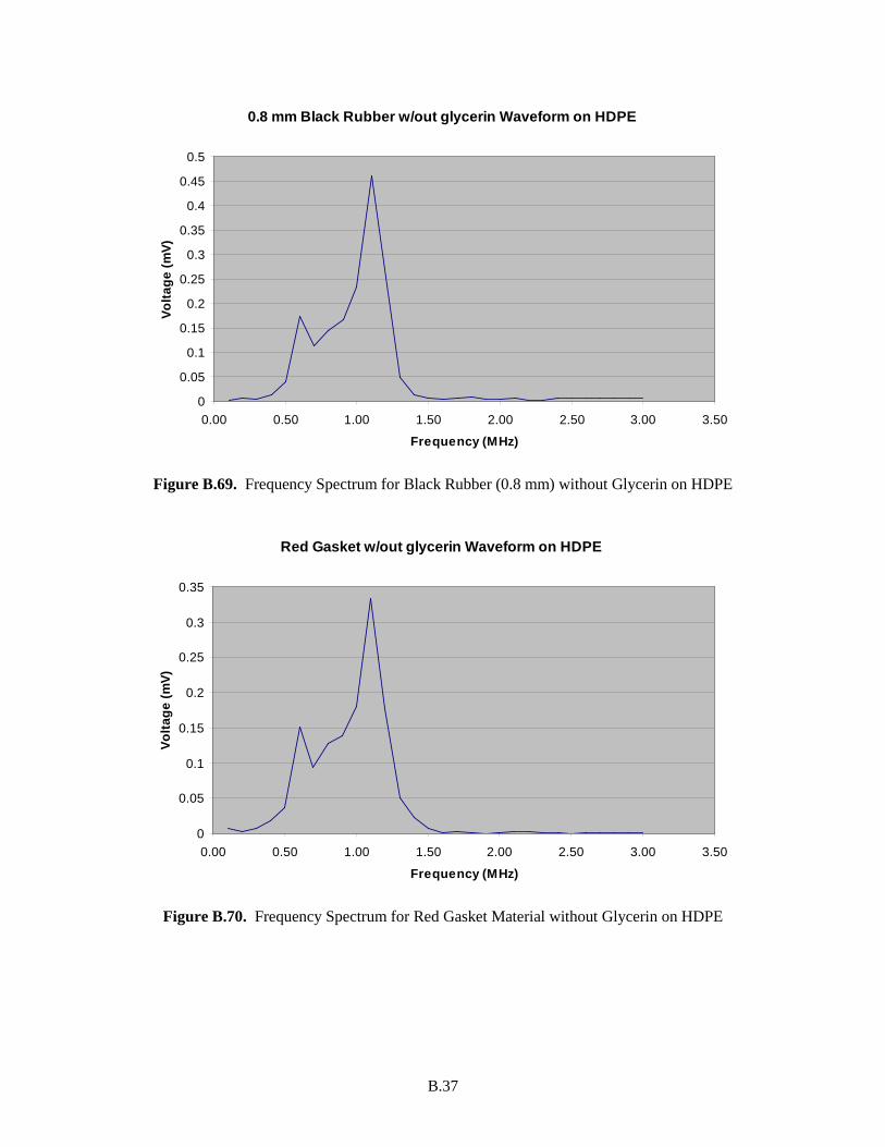
B.37
0.8 mm Black Rubber w/out glycerin Waveform on HDPE
0
0.05
0.1
0.15
0.2
0.25
0.3
0.35
0.4
0.45
0.5
0.00 0.50 1.00 1.50 2.00 2.50 3.00 3.50
Frequency (MHz)
Volta
ge (m
V)
Figure B.69. Frequency Spectrum for Black Rubber (0.8 mm) without Glycerin on HDPE
Red Gasket w/out glycerin Waveform on HDPE
0
0.05
0.1
0.15
0.2
0.25
0.3
0.35
0.00 0.50 1.00 1.50 2.00 2.50 3.00 3.50
Frequency (MHz)
Volta
ge (m
V)
Figure B.70. Frequency Spectrum for Red Gasket Material without Glycerin on HDPE
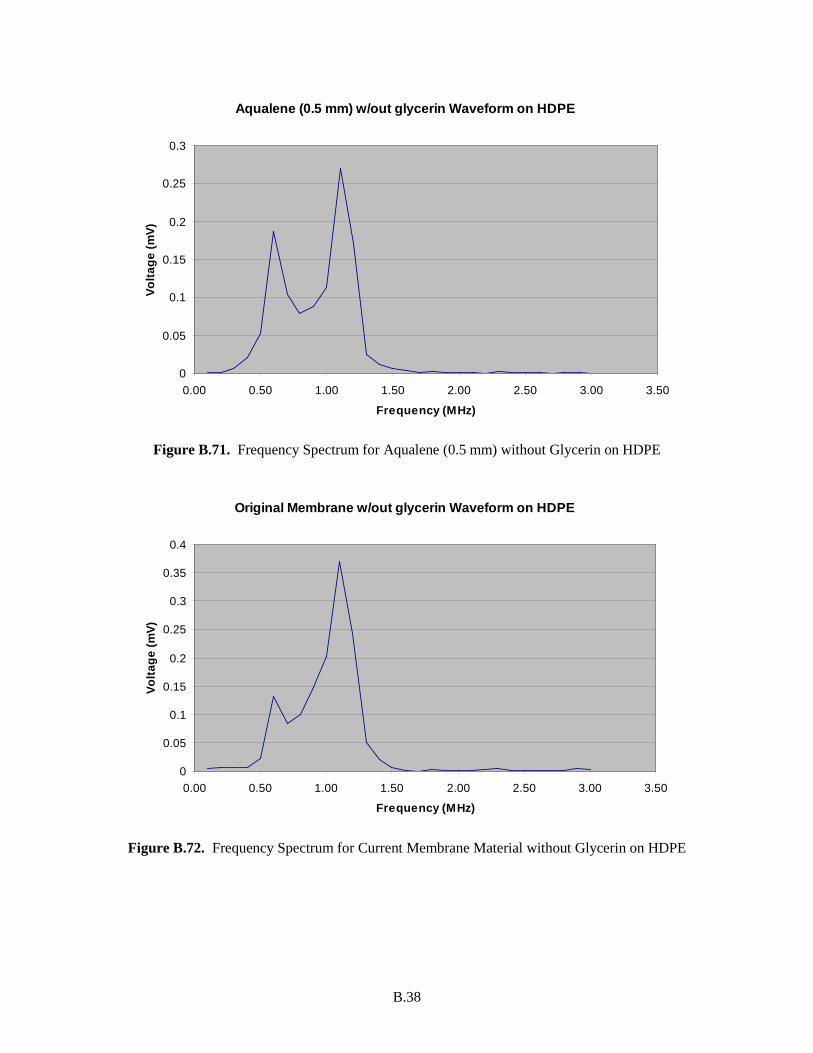
B.38
Aqualene (0.5 mm) w/out glycerin Waveform on HDPE
0
0.05
0.1
0.15
0.2
0.25
0.3
0.00 0.50 1.00 1.50 2.00 2.50 3.00 3.50
Frequency (MHz)
Volta
ge (m
V)
Figure B.71. Frequency Spectrum for Aqualene (0.5 mm) without Glycerin on HDPE
Original Membrane w/out glycerin Waveform on HDPE
0
0.05
0.1
0.15
0.2
0.25
0.3
0.35
0.4
0.00 0.50 1.00 1.50 2.00 2.50 3.00 3.50
Frequency (MHz)
Volta
ge (m
V)
Figure B.72. Frequency Spectrum for Current Membrane Material without Glycerin on HDPE

B.39
DCMA 1:2 w/out glycerin Waveform on HDPE
0
0.05
0.1
0.15
0.2
0.25
0.3
0.35
0.4
0.45
0.00 0.50 1.00 1.50 2.00 2.50 3.00 3.50
Frequency (MHz)
Volta
ge (m
V)
Figure B.73. Frequency Spectrum for DCMA 1:2 without Glycerin on HDPE
DCMA 1:1 w/out glycerin Waveform on HDPE
0
0.05
0.1
0.15
0.2
0.25
0.3
0.00 0.50 1.00 1.50 2.00 2.50 3.00 3.50
Frequency (MHz)
Volta
ge (m
V)
Figure B.74. Frequency Spectrum for DCMA 1:1 without Glycerin on HDPE
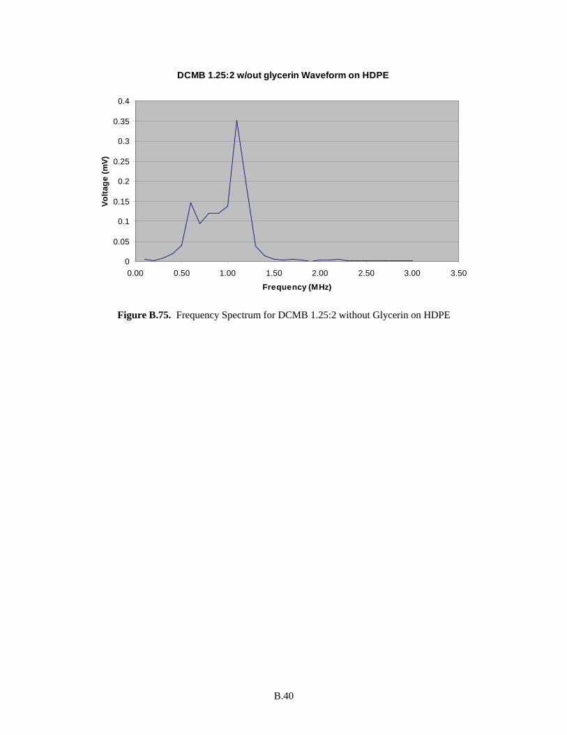
B.40
DCMB 1.25:2 w/out glycerin Waveform on HDPE
0
0.05
0.1
0.15
0.2
0.25
0.3
0.35
0.4
0.00 0.50 1.00 1.50 2.00 2.50 3.00 3.50
Frequency (MHz)
Volta
ge (m
V)
Figure B.75. Frequency Spectrum for DCMB 1.25:2 without Glycerin on HDPE

Appendix C
Acoustic Velocity-Temperature Profiles for all Liquids Characterized in Phase 2, and
Associated 2nd Order Polynomial Fit Equations

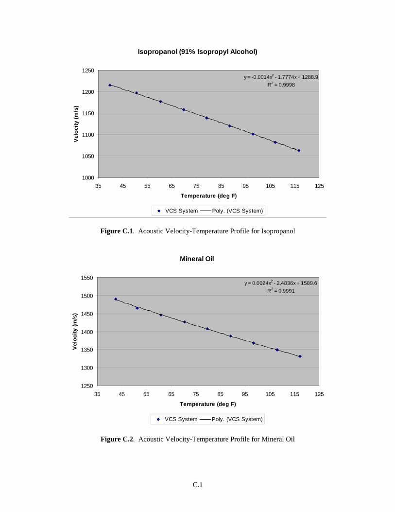
C.1
Isopropanol (91% Isopropyl Alcohol)
y = -0.0014x2 - 1.7774x + 1288.9R2 = 0.9998
1000
1050
1100
1150
1200
1250
35 45 55 65 75 85 95 105 115 125
Temperature (deg F)
Velo
city
(m/s
)
VCS System Poly. (VCS System)
Figure C.1. Acoustic Velocity-Temperature Profile for Isopropanol
Mineral Oil
y = 0.0024x2 - 2.4836x + 1589.6R2 = 0.9991
1250
1300
1350
1400
1450
1500
1550
35 45 55 65 75 85 95 105 115 125
Temperature (deg F)
Velo
city
(m/s
)
VCS System Poly. (VCS System)
Figure C.2. Acoustic Velocity-Temperature Profile for Mineral Oil
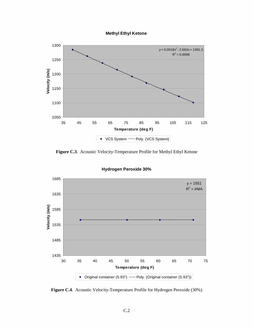
C.2
Methyl Ethyl Ketone
y = 0.0018x2 - 2.663x + 1391.3R2 = 0.9998
1050
1100
1150
1200
1250
1300
35 45 55 65 75 85 95 105 115 125
Temperature (deg F)
Velo
city
(m/s
)
VCS System Poly. (VCS System)
Figure C.3. Acoustic Velocity-Temperature Profile for Methyl Ethyl Ketone
Hydrogen Peroxide 30%
y = 1551R2 = #N/A
1435
1485
1535
1585
1635
1685
30 35 40 45 50 55 60 65 70 75
Temperature (deg F)
Velo
city
(m/s
)
Original container (5.93") Poly. (Original container (5.93"))
Figure C.4. Acoustic Velocity-Temperature Profile for Hydrogen Peroxide (30%)

C.3
Hydrogen Peroxide 35%
y = 1560.8R2 = #N/A
1435
1485
1535
1585
1635
1685
30 35 40 45 50 55 60 65 70 75
Temperature (deg F)
Velo
city
(m/s
)
Original container (5.93") Poly. (Original container (5.93"))
Figure C.5. Acoustic Velocity-Temperature Profile for Hydrogen Peroxide (35%)
Hydrogen Peroxide 50%
y = 1630R2 = #N/A
1485
1535
1585
1635
1685
1735
30 35 40 45 50 55 60 65 70 75
Temperature (deg F)
Velo
city
(m/s
)
Original container (5.93") Poly. (Original container (5.93"))
Figure C.6. Acoustic Velocity-Temperature Profile for Hydrogen Peroxide (50%)

C.4
Dioxane
y = -0.0024x2 - 1.9812x + 1507.6R2 = 0.9992
1050
1100
1150
1200
1250
1300
1350
1400
1450
35 55 75 95 115 135
Temperature (deg F)
Velo
city
(m/s
)
VCS System Poly. (VCS System)
Figure C.7. Acoustic Velocity-Temperature Profile for Dioxane
Chlorobenzene
y = 0.0015x2 - 2.3422x + 1438R2 = 0.9999
1050
1100
1150
1200
1250
1300
1350
1400
25 45 65 85 105 125
Temperature (deg F)
Velo
city
(m/s
)
VCS System Poly. (VCS System)
Figure C.8. Acoustic Velocity-Temperature Profile for Chlorobenzene

C.5
Acetyl Chloride
y = 0.0016x2 - 2.4315x + 1220.7R2 = 0.9998
920
970
1020
1070
1120
1170
25 45 65 85 105 125
Temperature (deg F)
Velo
city
(m/s
)
VCS System Poly. (VCS System)
Figure C.9. Acoustic Velocity-Temperature Profile for Acetyl Chloride

C.6
Appendix D
Excel Plots of Database Validation Data on Subset of Liquids for Various Containers across Multiple Temperature Points

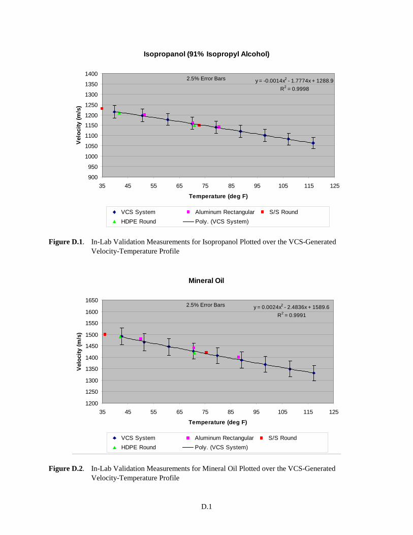
D.1
Isopropanol (91% Isopropyl Alcohol)
y = -0.0014x2 - 1.7774x + 1288.9R2 = 0.9998
900
950
1000
1050
1100
1150
1200
1250
1300
1350
1400
35 45 55 65 75 85 95 105 115 125
Temperature (deg F)
Velo
city
(m/s
)
VCS System Aluminum Rectangular S/S RoundHDPE Round Poly. (VCS System)
2.5% Error Bars
Figure D.1. In-Lab Validation Measurements for Isopropanol Plotted over the VCS-Generated
Velocity-Temperature Profile
Mineral Oil
y = 0.0024x2 - 2.4836x + 1589.6R2 = 0.9991
1200
1250
1300
1350
1400
1450
1500
1550
1600
1650
35 45 55 65 75 85 95 105 115 125
Temperature (deg F)
Velo
city
(m/s
)
VCS System Aluminum Rectangular S/S RoundHDPE Round Poly. (VCS System)
2.5% Error Bars
Figure D.2. In-Lab Validation Measurements for Mineral Oil Plotted over the VCS-Generated
Velocity-Temperature Profile

D.2
Methyl Ethyl Ketone
y = 0.0018x2 - 2.663x + 1391.3R2 = 0.9998
1000
1050
1100
1150
1200
1250
1300
1350
1400
1450
35 45 55 65 75 85 95 105 115 125
Temperature (deg F)
Velo
city
(m/s
)
VCS System Aluminum Rectangular S/S RoundHDPE Round Poly. (VCS System)
2.5% Error Bars
Figure D.3. In-Lab Validation Measurements for Methyl Ethyl Ketone Plotted over the VCS-Generated
Velocity-Temperature Profile
Dioxane
y = -0.0024x2 - 1.9812x + 1507.6R2 = 0.9992
1000
1100
1200
1300
1400
1500
1600
35 55 75 95 115 135
Temperature (deg F)
Velo
city
(m/s
)
VCS System Gold-Plated Rectangular Poly. (VCS System)
2.5% Error Bars
Figure D.4. In-Lab Validation Measurements for Dioxane Plotted over the VCS-Generated Velocity-
Temperature Profile

D.3
Chlorobenzene
y = 0.0015x2 - 2.3422x + 1438R2 = 0.9999
1050
1150
1250
1350
1450
1550
25 45 65 85 105 125
Temperature (deg F)
Velo
city
(m/s
)
VCS System Gold-Plated Rectangular Poly. (VCS System)
2.5% Error Bars
Figure D.5. In-Lab Validation Measurements for Chlorobenzene Plotted over the VCS-Generated
Velocity-Temperature Profile
Acetyl Chloride
y = 0.0016x2 - 2.4315x + 1220.7R2 = 0.9998
850
900
950
1000
1050
1100
1150
1200
1250
1300
1350
25 45 65 85 105 125
Temperature (deg F)
Velo
city
(m/s
)
VCS System Gold-Plated Rectangular Poly. (VCS System)
2.5% Error Bars
Figure D.6. In-Lab Validation Measurements for Acetyl Chloride Plotted over the VCS-Generated
Velocity-Temperature Profile

D.4