perspectives of jamming, mitigation and pattern adaptation ... · propose and evaluate strategies...
TRANSCRIPT

Perspectives of Jamming, Mitigation and Pattern Adaptation of
OFDM Pilot Signals for the Evolution of Wireless Networks
Raghunandan M. Rao
Thesis submitted to the Faculty of theVirginia Polytechnic Institute and State University
in partial fulfillment of the requirements for the degree of
Master of Sciencein
Electrical Engineering
Jeffrey H. Reed, ChairVuk Marojevic
Michael R. Buehrer
September 15, 2016Blacksburg, Virginia
Keywords: Multi-tone Pilot Jamming, Mitigation, OFDM systems, Long-Term Evolution(LTE)/LTE Cell-Specific Reference Signal (CRS) Jamming, Channel Quality Indicator (CQI)
Spoofing, Pilot Pattern AdaptationCopyright © 2016, Raghunandan M. Rao
Perspectives of Jamming, Mitigation and Pattern Adaptation of OFDM PilotSignals for the Evolution of Wireless Networks
Raghunandan M. Rao
(ABSTRACT)
Wireless communication networks have evolved continuously over the last four decades in orderto meet the traffic and security requirements due to the ever-increasing amount of traffic. Howeverthis increase is projected to be massive for the fifth generation of wireless networks (5G), with atargeted capacity enhancement of 1000×w.r.t. 4G networks. This enhanced capacity is possible bya combination of major approaches (a) overhaul of some parts and (b) elimination of overhead andredundancies of the current 4G. In this work we focus on OFDM reference signal or pilot tones,which are used for channel estimation, link adaptation and other crucial functions in Long-TermEvolution (LTE). We investigate two aspects of pilot signals pertaining to its evolution - (a) impactof targeted interference on pilots and its mitigation and (b) adaptation of pilot patterns to match thechannel conditions of the user.
We develop theoretical models that accurately quantify the performance degradation at the user’sreceiver in the presence of a multi-tone pilot jammer. We develop and evaluate mitigation al-gorithms to mitigate power-constrained multi-tone pilot jammers in SISO- and full rank spatial-multiplexing MIMO-OFDM systems. Our results show that the channel estimation performancecan be restored even in the presence of a strong pilot jammer. We also show that full rank spatialmultiplexing in the presence of a synchronized pilot jammer (transmitting on pilot locations only)is possible when the channel is flat between two pilot locations in either time or frequency.
We also present experimental results of multi-tone broadcast pilot jamming (Jamming of Cell-Specific Reference Signal) in the LTE downlink. Our results show that full-band jamming of pilotsneeds 5 dB less power than jamming the entire downlink signal, in order to cause Denial of Service(DoS) to the users. In addition to this, we have identified and demonstrated a previously unreportedissue with LTE termed ‘Channel Quality Indicator (CQI) Spoofing’. In this scenario, the attackertricks the user terminal into thinking that the channel quality is good, by transmitting interferencetransmission only on the data locations, while deliberately avoiding the pilots. This jammingstrategy leverages the dependence of the adaptive modulation and coding (AMC) schemes on theCQI estimate in LTE.
Lastly, we investigate the idea of pilot pattern adaptation for SISO- and spatial multiplexingMIMO-OFDM systems. We present a generic heuristic algorithm to predict the optimal pilotspacing and power in a nonstationary doubly selective channel (channel fading in both time andfrequency). The algorithm fits estimated channel statistics to stored codebook channel profiles anduses it to maximize the upper bound on the constrained capacity. We demonstrate up to a 30%improvement in ergodic capacity using our algorithm and describe ways to minimize feedback re-quirements while adapting pilot patterns in multi-band carrier aggregation systems. We concludethis work by identifying scenarios where pilot adaptation can be implemented in current wirelessnetworks and provide some guidelines to adapt pilots for 5G.
Perspectives of Jamming, Mitigation and Pattern Adaptation of OFDM PilotSignals for the Evolution of Wireless Networks
Raghunandan M. Rao
(GENERAL AUDIENCE ABSTRACT)
Wireless communications have evolved continuously over the last four decades in order to meet theever-increasing number of users. The next generation of wireless networks, named 5G, is expectedto interconnect a massive number of devices called the Internet of Things (IoT). Compared tothe current generation of wireless networks (termed 4G), 5G is expected to provide a thousand-fold increase in data rates. In addition to this, the security of these connected devices is also achallenging issue that needs to be addressed. Hence in the event of an attack, even if a tiny fractionof the total number of users are affected, this will still result in a large number of users who areimpacted.
The central theme of this thesis is the evolution of Orthogonal Frequency Division Multiplexing(OFDM) pilot signals on the road from 4G to 5G wireless networks. In OFDM, pilot signals aresent in parallel to data in order to aid the receiver in mitigating the impairments of the wirelesschannel. In this thesis, we look at two perspectives of the evolution of pilots: a) targeted inter-ference on pilot signals, termed as ‘Multi-tone pilot jamming’ and b) adapting pilot patterns tooptimize throughput.
In the first part of the thesis, we investigate the (a) impact of multi-tone pilot jamming and (b)propose and evaluate strategies to counter multi-tone pilot jamming. In particular, we proposemethods that (a) have the potential to be implemented in the Third Generation Partnership ProjectLong-Term Evolution (3GPP LTE) standard, and (b) have the ability to maintain high data rateswith a multi-antenna receiver, in the presence of a multi-tone pilot jammer. We also experimentand analyze the behavior of LTE in the presence of such targeted interference.
In the second half of the thesis, we explore the idea of adapting the density of pilots to optimizethroughput. Increasing the pilot density improves the signal reception capabilities, but reducesthe resources available for data and hence, data rate. Hence we propose and evaluate strategies tobalance between these two conflicting requirements in a wireless communication system.
In summary, this thesis provides and evaluates ideas to mitigate interference on pilot signals, anddesign data rate-maximizing pilot patterns for future OFDM-based wireless networks.
Acknowledgements
I am indebted to a lot of people for helping me successfully jumpstart my career in the area ofWireless Communications. Firstly, I would like to thank my mentors Dr. Jeffrey H. Reed andDr. Vuk Marojevic for giving me the opportunity, resources and the intellectual freedom to pursueinteresting ideas. I am deeply honored to work with prolific researchers such as yourself, and yourexpert guidance in the right direction has enabled me to focus on concrete research problems, andhelped me to formulate practical solutions in a timely manner.
I would also like to thank Dr. Michael R. Buehrer for serving on my thesis committee, and forhis helpful technical inputs. His course on ‘Multichannel Communications’ solidified my conceptsrelated to MIMO-OFDM, without which this thesis would have been difficult to accomplish.
I especially owe my gratitude to Dr. Harpreet Dhillon for motivating me during my first year ofgraduate study at Virginia Tech. His course on ‘Advanced Digital Communications’ introducedme to the exciting area of Communications, and led me to pursue research in Wireless Communi-cations.
I would also like to thank the Institute of Critical Technology and Applied Science (ICTAS), Vir-ginia Tech Foundation, Office of the Secretary of Defense (OSD), MS Technologies and OceusNetworks for funding my research and your support and cooperation.
To Dr. Eyosias Yoseph Imana: thanks for closely supervising my semester project in the courseon ‘Cellular Radios’, which formed the basis for this thesis. It was a great time working with youduring the Wireless@VT Symposium 2015. I learnt a lot from this single experience alone.
To Deven: I’m glad we got to work together the most during this year. It was a lot of fun workingwith you while preparing and presenting demos for visitors. You have been a great friend outsidework, and I will always cherish the times I spent with you.
To Randall: You have been the most pleasant person I’ve ever worked with. Your knowledge onRF and Microwave measurements has helped me a great deal while working on the experimentalpart of my thesis. To my colleagues Abid, Aditya, Kaleb, Marc, Matt, Miao, Mina, Munnawar,Sean, Tad and Xiaofu: you guys are awesome! It has been an enriching experience being a partof this group, bouncing ideas off of you guys and getting useful feedback. I hope to build morecollaborations with you guys in the future. Marc, Mina and Munnawar, it has been a pleasurecollaborating with you on LTE jamming and spectrum sharing research. I would also like to thank
iv

Sai Nisanth, Surabhi and Shankar for all your support and companionship.
To Hilda, Nancy and Joyce: thank you for constantly helping me navigate the logistics of gradschool.
I would also like to thank my current and former roommates: Abhishek, Prakhar, Abdus, Ajai andSteve for all the camaraderie. Grad school would have been very difficult without the support ofyou guys.
To my dear Swati: this transition would’ve been very stressful without you. Your never-endingoptimism and constant moral support has helped me remain strong during tough times. You havespread cheer everyday over these last two years. Thank you for everything.
To my beloved grandparents: you gave me the most beautiful childhood I could have ever wanted.Your absence will leave a void in my heart forever. I’ll always remember you through your lovefor the family, and the things you’ve taught me.
To my uncles Gururaj, Vasudev and Venkatesh: your constant moral support and fatherly advicehas always helped me believe in myself. I am blessed to have elders like you as a part of my family.
I am indebted to my parents and sister: I have missed home a lot, but am grateful for beingjust a phone call away. None of what I’ve accomplished would’ve been possible without yourunconditional love and unquestioning support. You are, and always will be the pillars of mystrength. Words aren’t enough to thank you for the life you’ve provided me with.
v

To my Family
vi
Contents
List of Figures xii
List of Tables xv
1 Introduction 1
1.1 Evolution of Wireless Networks . . . . . . . . . . . . . . . . . . . . . . . . . . . 1
1.2 Vulnerabilities of Wireless Networks . . . . . . . . . . . . . . . . . . . . . . . . . 2
1.3 Focus and Contributions of this Thesis . . . . . . . . . . . . . . . . . . . . . . . . 3
1.3.1 Contributions . . . . . . . . . . . . . . . . . . . . . . . . . . . . . . . . . 3
1.4 Organization of this Thesis . . . . . . . . . . . . . . . . . . . . . . . . . . . . . . 4
2 Theoretical Analysis of Multi-Tone Pilot Jamming in OFDM 6
2.1 Background . . . . . . . . . . . . . . . . . . . . . . . . . . . . . . . . . . . . . . 6
2.2 Channel Model . . . . . . . . . . . . . . . . . . . . . . . . . . . . . . . . . . . . 7
2.3 Channel Estimation . . . . . . . . . . . . . . . . . . . . . . . . . . . . . . . . . . 9
2.4 Mean Square Error (MSE) Analysis . . . . . . . . . . . . . . . . . . . . . . . . . 12
2.4.1 Mean Square Error in the Absence of a Jammer . . . . . . . . . . . . . . . 13
2.4.2 Mean Square Error in the Presence of a Synchronous Multi-Tone PilotJammer . . . . . . . . . . . . . . . . . . . . . . . . . . . . . . . . . . . . 16
2.4.3 Numerical Results . . . . . . . . . . . . . . . . . . . . . . . . . . . . . . 19
2.5 Bit Error Rate Analysis . . . . . . . . . . . . . . . . . . . . . . . . . . . . . . . . 19
2.5.1 BER in the Presence of a Synchronous Multi-Tone Pilot Jammer . . . . . . 22
vii
2.5.2 BER in the Absence of a Multi-Tone Pilot Jammer . . . . . . . . . . . . . 24
2.5.3 Numerical Results . . . . . . . . . . . . . . . . . . . . . . . . . . . . . . 24
2.6 Conclusions . . . . . . . . . . . . . . . . . . . . . . . . . . . . . . . . . . . . . . 27
3 Mitigation of Multi-Tone Pilot Jamming in SISO and MIMO-OFDM 28
3.1 Background . . . . . . . . . . . . . . . . . . . . . . . . . . . . . . . . . . . . . . 28
3.2 Types of Multi-Tone Pilot Jammers . . . . . . . . . . . . . . . . . . . . . . . . . . 29
3.3 Detection of Pilot Jamming . . . . . . . . . . . . . . . . . . . . . . . . . . . . . . 30
3.4 Anti-Jamming for SISO-OFDM Systems . . . . . . . . . . . . . . . . . . . . . . . 31
3.4.1 Resource Element Blanking with Interference Cancellation . . . . . . . . . 31
3.4.2 Cyclic Frequency Shifting of Pilot Locations . . . . . . . . . . . . . . . . 33
3.4.3 Numerical Results . . . . . . . . . . . . . . . . . . . . . . . . . . . . . . 33
3.5 Spatial Multiplexing with MIMO-OFDM in the Presence of Multi-Tone Pilot Jam-ming . . . . . . . . . . . . . . . . . . . . . . . . . . . . . . . . . . . . . . . . . . 35
3.5.1 Motivation . . . . . . . . . . . . . . . . . . . . . . . . . . . . . . . . . . 35
3.5.2 Channel Equalization in MIMO-OFDM . . . . . . . . . . . . . . . . . . . 39
3.5.3 Multi-Tone Pilot Jamming Model for MIMO-OFDM . . . . . . . . . . . . 42
3.5.4 Constant Channel Approximation (COCHAP) with Jammer Cancellation . 44
3.5.5 Numerical Results . . . . . . . . . . . . . . . . . . . . . . . . . . . . . . 47
3.6 Conclusions . . . . . . . . . . . . . . . . . . . . . . . . . . . . . . . . . . . . . . 52
4 Jamming of LTE’s Cell-Specific Reference Signal (CRS) 53
4.1 Background . . . . . . . . . . . . . . . . . . . . . . . . . . . . . . . . . . . . . . 53
4.2 The LTE Downlink . . . . . . . . . . . . . . . . . . . . . . . . . . . . . . . . . . 54
4.3 Channel Quality and Adaptive Modulation and Coding . . . . . . . . . . . . . . . 56
4.4 Impact of CRS Jamming on the Performance of LTE . . . . . . . . . . . . . . . . 56
4.4.1 Experimental Setup . . . . . . . . . . . . . . . . . . . . . . . . . . . . . . 57
4.4.2 Throughput Measurement Results . . . . . . . . . . . . . . . . . . . . . . 60
4.5 Conclusions . . . . . . . . . . . . . . . . . . . . . . . . . . . . . . . . . . . . . . 64
viii
5 Adaptation of Pilot Patterns for OFDM Systems 65
5.1 Introduction . . . . . . . . . . . . . . . . . . . . . . . . . . . . . . . . . . . . . . 65
5.2 Adaptation of Pilot Spacing and Power . . . . . . . . . . . . . . . . . . . . . . . . 66
5.2.1 Problem Formulation . . . . . . . . . . . . . . . . . . . . . . . . . . . . . 67
5.2.2 Estimation of Channel Statistics . . . . . . . . . . . . . . . . . . . . . . . 71
5.2.3 Channel Statistics Codebook . . . . . . . . . . . . . . . . . . . . . . . . . 71
5.2.4 Optimal Pilot Spacing and Power . . . . . . . . . . . . . . . . . . . . . . 72
5.2.5 Complexity . . . . . . . . . . . . . . . . . . . . . . . . . . . . . . . . . . 73
5.3 Numerical Results . . . . . . . . . . . . . . . . . . . . . . . . . . . . . . . . . . . 73
5.4 Some Practical Considerations for Pilot Adaptation in Current and Future WirelessNetworks . . . . . . . . . . . . . . . . . . . . . . . . . . . . . . . . . . . . . . . 81
5.5 Conclusions . . . . . . . . . . . . . . . . . . . . . . . . . . . . . . . . . . . . . . 82
6 Conclusions and Future Work 83
6.1 Thesis Summary and Conclusions . . . . . . . . . . . . . . . . . . . . . . . . . . 83
6.2 Future Work . . . . . . . . . . . . . . . . . . . . . . . . . . . . . . . . . . . . . . 84
6.2.1 Enhanced Mitigation Algorithms for Pilot Jamming . . . . . . . . . . . . . 84
6.2.2 Improving Resilience of LTE . . . . . . . . . . . . . . . . . . . . . . . . . 84
6.2.3 Cross-layer Optimization in Interference Channels . . . . . . . . . . . . . 85
6.2.4 Trust-Aware Protocol Design . . . . . . . . . . . . . . . . . . . . . . . . . 85
6.2.5 Pilot Pattern Adaptation . . . . . . . . . . . . . . . . . . . . . . . . . . . 85
A Additional Throughput Measurement Results 86
Bibliography 88
ix

List of Abbreviations
3GPP Third generation partnership projectAMC Adaptive modulation and codingBER Bit error rateBLER Block error rateCA Carrier aggregationCDF Cumulative distribution functionCOCHAP Constant channel approximationCoMP Cooperative MultipointCQI Channel quality indicatorCRS Cell-specific reference signalDoS Denial of serviceeNB Evolved node BFBMC Filter-bank multicarrierFDD Frequency division duplexFTN Faster than NyquistHARQ Hybrid automatic repeat requestICI Inter-carrier interferenceITU-T International Telecommunication Union - Telecommunication standardization sectorJC Jammer cancellationJSR Jammer to signal ratioLDPC Low density parity checkLS Least squaresLTE/LTE-A Long-term evolution/LTE advancedMCS Modulation and coding schemeMIMO Multiple input multiple outputMMSE Minimum mean squared errorMSE Mean square errorOFDM Orthogonal frequency division multiplexingPCFICH Physical control format indicator channelPCI Physical Cell IdentityPDSCH Physical downlink shared channelPHY Physical layer
x
PRACH Physical random access channelPSS Primary synchronization signalPUCCH Physical uplink control channelQAM Quadrature amplitude modulationQPSK Quadrature phase shift keyingRB Resource BlockRE Resource elementRF Radio frequencyS(I)NR Signal to (interference and) noise ratioSISO Single input single outputSSS Secondary synchronization signalTDD Time division duplexTTI Transmission time intervalUFMC Universal filtered multicarrierUAV Unmanned aerial vehicleUE User equipmentZF Zero forcing
xi

List of Figures
2.1 Mean Square Error analysis region for diamond-shaped pilot arrangement in OFDM. 10
2.2 Illustration of a Synchronous multi-tone pilot jammer. . . . . . . . . . . . . . . . . 18
2.3 Theoretical and simulated channel estimation Mean Square Error for fd = 100 Hz,τrms = 200 ns, in the case of a synchronous pulsed multi-tone pilot jammer. . . . . 20
2.4 Theoretical and simulated channel estimation Mean Square Error for fd = 200 Hz,τrms = 400 ns, in the case of a synchronous pulsed multi-tone pilot jammer. . . . . 20
2.5 Theoretical and simulated channel estimation Mean Square Error for fd = 500 Hz,τrms = 900 ns, in the case of a synchronous pulsed multi-tone pilot jammer. . . . . 21
2.6 Analysis Region for BER derivations in the presence and absence of a multi-tonepilot jammer. . . . . . . . . . . . . . . . . . . . . . . . . . . . . . . . . . . . . . 21
2.7 Theoretical and simulated BER performance of QPSK-OFDM for fd = 100 Hz,τrms = 200 ns,in the case of a synchronous pulsed multi-tone pilot jammer. . . . . 25
2.8 Theoretical and simulated BER performance of QPSK-OFDM for fd = 200 Hz,τrms = 400 ns,in the case of a synchronous pulsed multi-tone pilot jammer. . . . . 25
2.9 Theoretical and simulated BER performance of QPSK-OFDM for fd = 500 Hz,τrms = 900 ns, in the case of a synchronous pulsed multi-tone pilot jammer. . . . . 26
3.1 Mitigation of asynchronous multi-tone pilot jamming by resource element blank-ing with interference cancellation. . . . . . . . . . . . . . . . . . . . . . . . . . . 32
3.2 Mitigation of synchronous multi-tone pilot jamming by cyclic frequency shiftingof pilot locations. . . . . . . . . . . . . . . . . . . . . . . . . . . . . . . . . . . . 32
3.3 Channel Estimation MSE performance of QPSK-OFDM in all considered scenar-ios, for τrms = 200 ns, fd = 100 Hz. . . . . . . . . . . . . . . . . . . . . . . . . . 36
3.4 Channel Estimation MSE performance of QPSK-OFDM in all considered scenar-ios, for τrms = 400 ns, fd = 200 Hz. . . . . . . . . . . . . . . . . . . . . . . . . . 36
xii

3.5 Channel Estimation MSE performance of QPSK-OFDM in all considered scenar-ios, for τrms = 900 ns, fd = 500 Hz. . . . . . . . . . . . . . . . . . . . . . . . . . 37
3.6 Bit Error rate performance of QPSK-OFDM in all considered scenarios, for τrms =200 ns, fd = 100 Hz. . . . . . . . . . . . . . . . . . . . . . . . . . . . . . . . . . 37
3.7 Bit Error rate performance of QPSK-OFDM in all considered scenarios, for τrms =400 ns, fd = 200 Hz. . . . . . . . . . . . . . . . . . . . . . . . . . . . . . . . . . 38
3.8 Bit Error rate performance of QPSK-OFDM in all considered scenarios, for τrms =900 ns, fd = 500 Hz. . . . . . . . . . . . . . . . . . . . . . . . . . . . . . . . . . 38
3.9 Diamond-shaped pilot pattern for 4× 4 MIMO-OFDM. . . . . . . . . . . . . . . 41
3.10 Illustration of synchronous multi-tone pilot jamming in a 4 × 4 MIMO-OFDMblock, for all spatial layers. . . . . . . . . . . . . . . . . . . . . . . . . . . . . . . 43
3.11 Schematic of the Constant Channel Approximation (COCHAP) assumption forpilots from transmit antenna 1 for j = 1, 2, 3, 4. . . . . . . . . . . . . . . . . . . . 43
3.12 Comparison of Ergodic sum capacity for all scenarios, for τrms = 100 ns, fd = 50 Hz. 49
3.13 Comparison of Ergodic sum capacity for all scenarios, for τrms = 200 ns, fd =100 Hz. . . . . . . . . . . . . . . . . . . . . . . . . . . . . . . . . . . . . . . . . 49
3.14 Comparison of Ergodic sum capacity for all scenarios, for τrms = 400 ns, fd =200 Hz. . . . . . . . . . . . . . . . . . . . . . . . . . . . . . . . . . . . . . . . . 50
3.15 Comparison of Bit Error Rate for all scenarios, for τrms = 100 ns, fd = 50 Hz. . . . 50
3.16 Comparison of Bit Error Rate for all scenarios, for τrms = 200 ns, fd = 100 Hz. . . 51
3.17 Comparison of Bit Error Rate for all scenarios, for τrms = 400 ns, fd = 200 Hz. . . 51
4.1 A 1.4 MHz FDD-LTE downlink frame normal cyclic prefix, corresponding to an-tenna port 0 of the eNodeB. . . . . . . . . . . . . . . . . . . . . . . . . . . . . . . 54
4.2 Schematic of the experimental setup for throughput measurements of the LTEDownlink. . . . . . . . . . . . . . . . . . . . . . . . . . . . . . . . . . . . . . . . 59
4.3 Schematic of the jamming strategies investigated for throughput performance ofthe LTE downlink. The number of REs affected are the same in CRS and datasubcarrier jamming. . . . . . . . . . . . . . . . . . . . . . . . . . . . . . . . . . 60
4.4 Measured throughput versus JSR per Resource Block for all considered jammingschemes. . . . . . . . . . . . . . . . . . . . . . . . . . . . . . . . . . . . . . . . . 61
xiii

4.5 Comparison of maximum theoretically achievable (Rmax,MCS), and measured av-erage (Rmeas) throughput values versus JSR per Resource Block, for (a) CRS jam-ming, (b) data subcarrier jamming (1 out of 3 data subcarriers above/below CRSfrequencies), and (c) barrage jamming. . . . . . . . . . . . . . . . . . . . . . . . . 63
4.6 Comparison of achievable throughput efficiency (ηach,th) for all considered cases. . 63
5.1 Illustration of pilot adaptation based on varying channel conditions. . . . . . . . . 68
5.2 Scenario of channel statistics variation for all cases. . . . . . . . . . . . . . . . . . 76
5.3 Ergodic Capacity Performance in SISO-OFDM for all considered pilot configura-tions. . . . . . . . . . . . . . . . . . . . . . . . . . . . . . . . . . . . . . . . . . . 77
5.4 The CDF of Capacity for pilot adaptation versus LTE spacing, ρ = −3 dB forSISO-OFDM. . . . . . . . . . . . . . . . . . . . . . . . . . . . . . . . . . . . . . 77
5.5 Capacity gain of pilot adaptation versus the other considered fixed pilot configura-tions for SISO-OFDM. . . . . . . . . . . . . . . . . . . . . . . . . . . . . . . . . 78
5.6 Ergodic Capacity Performance in MIMO-OFDM for all considered pilot configu-rations. . . . . . . . . . . . . . . . . . . . . . . . . . . . . . . . . . . . . . . . . 78
5.7 The CDF of capacity for pilot adaptation versus LTE spacing, ρ = −3 dB forMIMO-OFDM. . . . . . . . . . . . . . . . . . . . . . . . . . . . . . . . . . . . . 79
5.8 Capacity gain of pilot adaptation versus the other considered fixed pilot configura-tions for MIMO-OFDM. . . . . . . . . . . . . . . . . . . . . . . . . . . . . . . . 79
xiv
List of Tables
2.1 Description of the most important parameters . . . . . . . . . . . . . . . . . . . . 8
2.2 Simulation Parameters . . . . . . . . . . . . . . . . . . . . . . . . . . . . . . . . 18
2.3 Relationship between JSR (dB) and ρ. . . . . . . . . . . . . . . . . . . . . . . . . 26
3.1 Important Symbols and Notation . . . . . . . . . . . . . . . . . . . . . . . . . . . 40
4.1 Mapping from CQI to spectral efficiency for 3GPP LTE Release 8. Adapted from[1]. . . . . . . . . . . . . . . . . . . . . . . . . . . . . . . . . . . . . . . . . . . . 57
4.2 Mapping from MCS to Maximum Throughput of Physical Downlink Shared Chan-nel (PDSCH) for a FDD SISO 10MHz LTE Release 8 Downlink. Adapted from[2]. . . . . . . . . . . . . . . . . . . . . . . . . . . . . . . . . . . . . . . . . . . . 58
4.3 Parameters of the LTE Downlink Throughput measurement setup. . . . . . . . . . 59
5.1 Description of the most important parameters . . . . . . . . . . . . . . . . . . . . 69
5.2 Codebook of Channel Profiles,RC . . . . . . . . . . . . . . . . . . . . . . . . . . 74
5.3 Capacity gains of pilot adaptation w.r.t. fixed pilot configurations: comparisonagainst state of the art . . . . . . . . . . . . . . . . . . . . . . . . . . . . . . . . . 81
A.1 Summary of statistics of measured throughput in the LTE jamming experiments. . . 87
xv
Chapter 1
Introduction
1.1 Evolution of Wireless Networks
Wireless networks have evolved over the last four decades, from the first generation (1G) analogstandards in the 1980s to the current digital fourth generation (4G) networks which saw worldwidedeployment over the last couple of years. In each generation, there has been major upgradesover its predecessors in terms of coverage, speed, services etc. We are currently on the brink ofthe standardization of fifth generation (5G) wireless networks that are expected to provide 1000×capacity w.r.t. 4G networks, along with other performance enhancements such as ultra-low latency;and interconnecting a massive number of devices to the Internet, called the Internet of Things (IoT).
The Third Generation Partnership Project (3GPP) has standardized the Long-Term Evolution (LTE)from Release 8 in 2009 to Release 13 in 2016 [3]. The next version (Release 14) is scheduled forcompletion by 2017. There have been addition of new features in the latest two releases of LTEcompared to the initial releases. Some of the important features introduced in these are support forhigher order modulation schemes (256QAM), higher number of spatial layers (up to 8×8 MIMO),throughput enhancements using Carrier Aggregation (CA), cell-edge coverage enhancements us-ing Cooperative Multi-point (CoMP) etc. The wireless evolution from 4G to 5G is expected tohappen through a combination of the following approaches: (a) major system overhaul of someaspects of 4G and (b) elimination of redundancies, and upgrades to LTE. Some of the promisingtechnologies actively researched for 5G wireless networks are:
(a) Millimeter-wave (mmWave) communications [4],
(b) Massive MIMO [4],
(c) Alternatives to OFDM: Filter-bank Multicarrier (FBMC), Universal Filtered Multicarrier(UFMC), Faster than Nyquist (FTN) etc. [5],
(d) Machine-Type Communications (MTC), and many more.
1
Raghunandan M. Rao Chap 1. Introduction 2
Broadly, the recurrent theme in several 5G proposals is support for parameter adaptation in thesystem, be it subcarrier spacing, cyclic prefix, pulse shape or others [6]. This is meant to optimizethe system performance based on the operating conditions of the network like channel statistics,traffic patterns.
Pilot signals have traditionally been designed to have a fixed pattern in order to avoid complexity.But they represent an essential overhead in the system since they do not carry data symbols. Be-cause of the heterogeneity of the user mobilities and channel characteristics in a practical scenario,dense pilot patterns become an unnecessary overhead if the channel remains flat enough in timeor frequency. In this regard, this thesis explores the idea of adaptation of downlink pilot pattern inorder to maximize the capacity of the system based on feedback of channel statistics from the userto the base station.
In addition to performance enhancements, superior levels of reliability and security is also neces-sary since in 5G networks it is expected to support critical infrastructure, in addition to civilian andmilitary user traffic.
1.2 Vulnerabilities of Wireless Networks
Security and privacy has always been an evolving problem in the area of wireless communicationssince the days of the analog 1G cellular network. Each cellular generation has undergone its shareof research and development related to wireless network attacks and countermeasures becauseeach new feature introduced can have a potential vulnerability can be exploited by an attacker. Theimportance of wireless security is and will be even more important in the future because criticalsystems such as public safety, national security, commercial and military communications willdepend on the reliability of a wireless network.
The limits of wireless security will be tested in a 5G wireless network, simply because of the sheervolume and density of the devices that is expected to be served by the network. Affecting a tinyfraction of this number would result in the loss of functionality of a massive number of devices.Hence, the importance of making current and future wireless networks more robust to attacks andfailures cannot be understated. Standardization of 5G networks is a couple of years away fromtaking form. Therefore, this thesis deals with the resilience of LTE networks and its downlinkphysical layer technology, Orthogonal Frequency Division Multiplexing. Prior research [7, 8] hasshown that targeted interference on pilot signals is more efficient in degrading the Bit Error Rateperformance than full-band jamming (also known as Barrage Jamming). Hence, this thesis willspecifically be investigating and quantifying the impact of targeted interference on pilot signals,developing countermeasures against such attacks, and testing the resilience of the LTE downlinkto such attacks.
Raghunandan M. Rao Chap 1. Introduction 3
1.3 Focus and Contributions of this Thesis
This thesis investigates the evolution of pilot signals, on the road from 4G to 5G wireless networks.The main ideas of focus are:
1. Vulnerability of OFDM downlink pilot signals to targeted interference, i.e. multi-tone pilotjamming.
2. Mitigation strategies to make OFDM systems more robust to multi-tone pilot jamming.
3. Study of the effect of targeted interference on LTE downlink pilots and (or) data resourceelements.
4. Adaptation of OFDM downlink pilot pattern based on changing wireless channel character-istics
We provide important lessons learned from our investigation of OFDM systems in general, andLTE in particular. Our findings can help in the robust design of future 5G wireless networks toprovide resilience against intentional and unintentional interference.
1.3.1 Contributions
The contribution of this thesis is divided into three parts. The first part develops a framework foranalyzing multi-tone pilot jamming of downlink pilots in OFDM systems. OFDM is the underlyingbaseline communications technology for the LTE air interfaces. Hence, the second part appliesthe analysis to LTE-specific control channels and performance metrics. Finally, we propose analgorithm to adapt the pilot structure to optimize communications performance as a function ofchannel conditions.
1.3.1.1 Multi-Tone Pilot Jamming and Mitigation in OFDM Systems
Multi-tone pilot jamming refers to deliberate transmission of interference on top of pilot signalsthat degrade the process of equalization in coherent detection receivers. Prior research [9, 7, 8, 10,11, 12, 13] has investigated pilot jamming and its mitigation in OFDM systems. This thesis buildson this body of work to quantify and demonstrate the level of degradation
(a) We develop a mathematical formulation and derive the Bit Error Rate (BER) and channelEstimation Mean Square Error (MSE) expressions for time and frequency fading channels(also known as doubly dispersive/selective channels).

Raghunandan M. Rao Chap 1. Introduction 4
(b) We introduce and evaluate mitigation strategies for power-constrained pilot jammers inSISO-OFDM systems. In contrast to prior work, the proposed mitigation strategies are morepractical and simpler to be implemented in the widely deployed LTE networks.
(c) We devise and assess the performance of an approximate channel estimation algorithm inthe presence of a power-constrained pilot jammer for MIMO-OFDM with full rank spatialmultiplexing. As opposed to prior research in [13], we consider a the scenario where thepilots are broadcasted to the users of the cell and channel estimates are imperfect. Theapproximation is shown to yield satisfactory results in outdoor to indoor/indoor to indoorchannels [14], and can be used for slow fading channels as well.
1.3.1.2 CRS Jamming and CQI Spoofing in LTE
Recently, research in [15, 16, 17, 18, 19] has looked at various control channel attacks in LTE. Thisthesis extends this body of research by analyzing the impact of CRS Jamming and CQI spoofing inthe LTE downlink. Cell-Specific Reference Signals (CRS) are the downlink pilots in LTE, whileChannel Quality Indicator (CQI) indicates the quality of the channel based on which the eNodeB(LTE Base Station) adapts its modulation scheme and rate of error control coding. To the best ofour knowledge, we have demonstrated ‘CQI Spoofing’ in LTE for the first time, wherein a jammertricks the user into believing that the channel quality is good even though it isn’t, by targetinginterference on data subcarriers only. Experimental results pertaining to CRS Jamming and CQIspoofing are demonstrated, and its implications are discussed in this work.
1.3.1.3 Pilot Pattern Adaptation for Throughput Maximization
Current wireless networks use fixed pilot patterns, which lead to unnecessary overhead if the chan-nel is flat in either time or frequency. Hence, it makes sense to adapt pilot patterns based on thechannel flatness as seen by the user. Prior work has investigated and demonstrated pilot adaptationfor MIMO-OFDM systems, and has compared its throughput performance with respect to that ofLTE’s fixed pilot pattern. Our work has built on this idea, and we have devised a simple codebookbased approach to adapt pilot spacing in time and frequency in doubly dispersive channels. Weshow the throughput gains w.r.t. fixed pilot spacing, and provide insights for its extension intomulti-band carrier aggregation systems with reduced feedback requirements. We also discuss theconditions which are necessary to implement pilot pattern adaptation.
1.4 Organization of this Thesis
Chapter 2 presents the system model and the mathematical derivation of the theoretical BER andchannel estimation MSE in the presence of a multi-tone pilot jammer. Chapter 3 deals with mit-
Raghunandan M. Rao Chap 1. Introduction 5
igation techniques to counter a power-constrained multi-tone pilot jammer in SISO- and MIMO-OFDM systems. Chapter 4 demonstrates the impact of CRS Jamming and CQI Spoofing in theLTE downlink. Chapter 5 presents a heuristic algorithm to adapt pilot spacing in time and fre-quency based on estimated channel statistics, for SISO- and MIMO-OFDM scenarios. Finally,Chapter 6 provides the main conclusions, with a brief discussion of the research directions that canbe spawned out of this work.
Chapter 2
Theoretical Analysis of Multi-Tone PilotJamming in OFDM
2.1 Background
Orthogonal Frequency Division Multiplexing (OFDM) is pervasive in today’s wireless networks.The reason for its popularity is due to (a) its ability to achieve high data rates in mobile environ-ments by effectively dealing with multipath propagation (b) tight channel packing (c) high areaspectral efficiency (d) flexible resource allocation flexibility and scalability and (e) compatibilitywith multi-antenna techniques. It is employed in wireless commercial communications standards,such as IEEE 802.11 and LTE. It will be used for next-generation public safety networks and othermission critical communications systems [20].
OFDM waveforms and communications systems that use it have been analyzed in terms of robust-ness against radio frequency (RF) interference of various types. Research results have shown thatOFDM-based systems are vulnerable to targeted RF interference [8, 9, 12, 21]. Although this kindof interference can be caused by an adversary that tries to disrupt communications, it can also becaused by other wireless systems in shared or unlicensed bands. Systems and technology needto adapt to the emerging scenario of shared, rather than exclusive use of spectrum for commer-cial wireless, including cellular communications. Hence, it is crucial to address the physical layervulnerabilities of OFDM.
When the interferer has no prior knowledge about the signaling structure in the network, widebandbarrage jamming is shown to be optimal [22]. The open access to wireless standards documenta-tion makes it easy for an adversary to do better than wideband barrage jamming. Prior research [7],[8] has shown that OFDM reference signal or pilot-tone jamming is more efficient than widebandjamming. This is so because excessive interference on the reference signal corrupts the channelestimates, which are typically obtained by interpolating between the channel estimates of two ormore reference symbols [23]. Hence, the equalization process is disrupted and the data demodula-
6
Raghunandan M. Rao Chap. 2 Theoretical Analysis of Multi-Tone Pilot Jamming in OFDM 7
tion performance is degraded for relatively lower powers as compared to wideband jamming.
Patel et al. [9] derived closed form BER expressions to study the effect of imperfect channel es-timation for OFDM/MC-CDMA systems in frequency-selective Rayleigh fading channels, in thepresence and absence of a jammer. Han et al. [10] analyzed the mean squared error (MSE) ofchannel estimation in the presence of a narrowband pilot jammer and propose a jammed pilot de-tection and excision algorithm to mitigate the jammer. The damage that single-tone pilot jammingcan cause is limited since only the adjacent data-carrying subcarriers would be affected.
Jun et al. [24] analyzed the BER performance under various partial-band, full-band and multi-tonejammer configurations for BPSK- and DBPSK-OFDM systems. Jasmin and Clancy [11] have de-rived closed-form expressions for PSK-OFDM and PSK-Single Carrier FDMA (PSK-SC FDMA)systems in the presence of jamming and imperfect channel estimation. These works assume apilot-structure that requires time-only or frequency-only interpolation for channel estimation.
We extend on prior work and derive the MSE and BER for OFDM systems in doubly selectivechannels (strong fading in time and frequency), both in the presence and absence of a multi-tonepilot jammer. We assume a ‘diamond-shaped’ pilot arrangement for the OFDM block, becauseequal spacing of pilots in the block achieves the minimum MSE (MMSE) estimate of the channel[25]. This arrangement of pilots is used in modern communication systems, like 3GPP LTE/LTE-A. We assume least squares (LS) channel estimation along with linear interpolation for channelequalization because of its low complexity and good performance in the MSE sense, making itattractive for practical implementations [26].
Section 2.2 describes the system model for the wireless channel. Section 2.3 outlines the channelestimation algorithm in the presence and absence of a multi-tone pilot jammer. Section 2.4 presentsthe derivation and numerical simulation results of the MSE expressions for SISO-OFDM systems.Section 2.5 presents the derivation and numerical simulation results of the BER expressions. Sec-tion 2.6 concludes by summarizing the main results of this chapter.
Notation
The most important parameters and variables used in this chapter is introduced in Table 2.1.
2.2 Channel Model
The channel impulse response (CIR) h(t, τ) of a mobile wireless channel can be written as
h(t, τ) =∑i
γi(t)δ(τ − τi), (2.1)
where τi is the delay of the ith resolvable multipath component, γi(t) its corresponding complexamplitude and δ(t) the Dirac delta function. Due to relative motion in the channel, the γi(t)’s are

Raghunandan M. Rao Chap. 2 Theoretical Analysis of Multi-Tone Pilot Jamming in OFDM 8
Table 2.1: Description of the most important parameters
Variable Descriptionσ2H Channel power gain factorRt(∆t) Temporal correlation function of the wireless channelRf (∆f) Frequency correlation function of the wireless channelτrms Root mean square delay spread of the wireless channelfd Maximum Doppler Spread (Hz)vtr Relative speed between the transmitter and the receiverfc Center frequency of the OFDM signalσ2w Noise varianceσ2p Pilot signal powerN Total number of subcarriers per OFDM symbolL Pilot spacing in frequency on the same OFDM symboltp Pilot spacing in time between two consecutive pilot-bearing OFDM symbolsT Pilot spacing in time between two odd/even-numbered pilot-bearing OFDM symbolsHk[n] Actual channel co-efficient of the kth subcarrier on the nth OFDM symbolHk[n] Channel estimate of the kth subcarrier on the nth OFDM symbolP Set of pilot locations in the OFDM block. Its elements are of the form n, k ∈ P|P| Number of pilot locations in the OFDM frameγb Average SNR per bit of QPSK symbolsPb(n, k) Probability of bit error at the kth subcarrier on the nth OFDM symbol
wide-sense stationary (WSS) narrowband complex Gaussian processes, and each γi(t) is indepen-dent of the other multipath components γj(t) for i 6= j [27]. We model all γi(t)’s to have the samenormalized correlation function Rt(∆t) given by
rγi(∆t) = E[γi(t+ ∆t)γ∗i (t)] = σ2iRt(∆t), (2.2)
where E[·] denotes the statistical expectation and σ2i the average power of the ith signal path. The
channel frequency response (CFR) H(t, f) is the Fourier transform of the CIR and is given by
H(t, f) =
∫ +∞
−∞h(t, τ)e−j2πftdτ =
∑i
γi(t)e−j2πfτi . (2.3)
The CFR can be used to compute the correlation function RH(∆t,∆f) that describes the secondorder statistics of the channel. It is defined as
RH(∆t,∆f) , E[H(t+ ∆t, f + ∆f)H∗(t, f)]. (2.4)
Raghunandan M. Rao Chap. 2 Theoretical Analysis of Multi-Tone Pilot Jamming in OFDM 9
Using equations (2.1)-(2.4), we can rewrite (2.4) as [27]
RH(∆t,∆f) = E[∑
i
γi(t+ ∆t)e−j2π(f+∆f)τi]×[∑
i
γ∗i (t)ej2πfτi
]=∑i
E[γi(t+ ∆t)γ∗i (t)]e−j2π∆fτi
=∑i
σ2iRt(∆t)e
−j2π∆fτi
= Rt(∆t)∑i
σ2i e−j2π∆fτi . (2.5)
If we consider σ2H =
∑i σ
2i , we can define the channel frequency correlation function Rf (∆f) as
Rf (∆f) ,∑i
σ2i
σ2H
e−j2π∆fτi . (2.6)
Using this result, we can decompose the channel correlation function into its time and frequencycorrelation components:
RH(∆t,∆f) = σ2HRt(∆t)Rf (∆f). (2.7)
For simplicity, we assume a channel with σ2H = 1 in this work. Equation (2.7) is widely known as
the ‘Wide Sense Stationary Uncorrelated Scattering’ (WSSUS) approximation that enables the useof two 1-D estimators for channel estimation instead of the more complex 2-D estimators for jointtime-frequency channel estimation in OFDM. The temporal correlation function Rt(∆t) is givenby the Jakes’ model [28]
Rt(∆t) = J0(2πfd∆t), (2.8)
where J0(·) is the Bessel function of the first kind of zeroth order, fd = vtrfc/c with vtr being therelative speed between the transmitter and the receiver, fc the carrier frequency, and c the speed oflight in free space.
2.3 Channel Estimation
Pilots are sent in parallel with data on dedicated time-frequency components of the OFDM block,called as a Resource Element (RE). We assume that the OFDM resource blocks have a ‘diamond-shaped’ arrangement of pilots because this arrangement achieves the MMSE estimate of the chan-nel [25]. This pilot arrangement is used in the 3GPP LTE/LTE-A standard. Figure 2.1 shows thetime-frequency resource grid, consisting of resource elements (REs) that form regular block struc-tures. Each RE carries a modulation symbol (data) or a pilot symbol. Here, the pilot period isT seconds on the time axis and L subcarriers on the frequency axis with a cyclic frequency shiftof L/2 between two consecutive pilot-bearing OFDM symbols. The analysis region is indicated

Raghunandan M. Rao Chap. 2 Theoretical Analysis of Multi-Tone Pilot Jamming in OFDM 10
𝑇
𝑡𝑝
𝑇 − 𝑡𝑝
𝐿
2+ 1
𝐿
2− 1
Type – A subcarriers
subregion 2 - right
subregion 1 - right
subregion 1 - left
subregion 2 - left
pilots
(P-1)
subcarriers
(Q-1)
subcarriers
(L-1)
subcarriers Type – B subcarriers
Type – C subcarriers
fre
qu
en
cy
time
Figure 2.1: Mean Square Error analysis region for diamond-shaped pilot arrangement in OFDM.
by the colored REs in Figure 2.1, which periodically repeats in time and frequency to form theOFDM resource block. The analysis region forms a basis for the OFDM resource block, and hencethe problem of MSE analysis of the OFDM block can be simplified to that of the analysis region.Sub-region 1 refers to the bottom (L/2 + 1) subcarriers and sub-region 2 to the top (L/2− 1) sub-carriers of the analysis region. Without loss of generality, we assume that L is an even number. Tosimplify the performance analysis, we divide the OFDM block into four distinct types of resourceelements:
1. Pilots: Their channel estimates are obtained using Least Squares (LS) channel estimation, asshown in equation (2.10).
2. Type A: Resource Elements that lie between 2 pilot subcarriers. Their channel estimatesare obtained by interpolation of channel estimates in frequency, between these two pilotsubcarriers, as shown in equation (2.11) - (2.12), with t = 0.
3. Type B and C: Subcarriers that lie after the last pilot subcarrier (Type B), or before the firstpilot subcarrier (Type C). Their channel estimates are obtained by extrapolation of channelestimates in frequency, using the ultimate and penultimate pilots (Type B) and the first andsecond pilots (Type C).
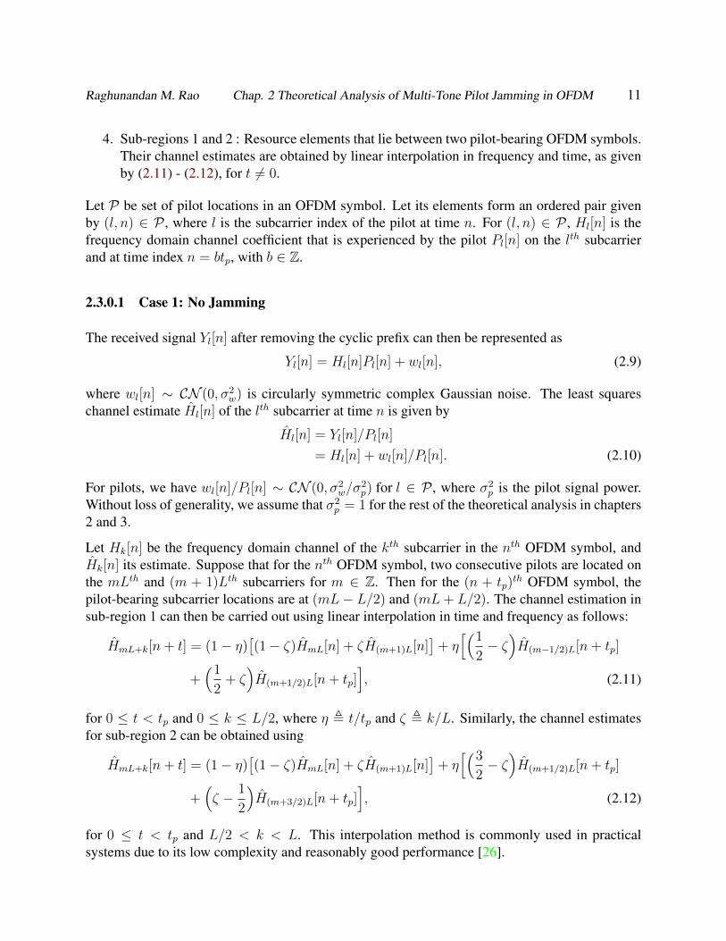
Raghunandan M. Rao Chap. 2 Theoretical Analysis of Multi-Tone Pilot Jamming in OFDM 11
4. Sub-regions 1 and 2 : Resource elements that lie between two pilot-bearing OFDM symbols.Their channel estimates are obtained by linear interpolation in frequency and time, as givenby (2.11) - (2.12), for t 6= 0.
Let P be set of pilot locations in an OFDM symbol. Let its elements form an ordered pair givenby (l, n) ∈ P , where l is the subcarrier index of the pilot at time n. For (l, n) ∈ P , Hl[n] is thefrequency domain channel coefficient that is experienced by the pilot Pl[n] on the lth subcarrierand at time index n = btp, with b ∈ Z.
2.3.0.1 Case 1: No Jamming
The received signal Yl[n] after removing the cyclic prefix can then be represented as
Yl[n] = Hl[n]Pl[n] + wl[n], (2.9)
where wl[n] ∼ CN (0, σ2w) is circularly symmetric complex Gaussian noise. The least squares
channel estimate Hl[n] of the lth subcarrier at time n is given by
Hl[n] = Yl[n]/Pl[n]
= Hl[n] + wl[n]/Pl[n]. (2.10)
For pilots, we have wl[n]/Pl[n] ∼ CN (0, σ2w/σ
2p) for l ∈ P , where σ2
p is the pilot signal power.Without loss of generality, we assume that σ2
p = 1 for the rest of the theoretical analysis in chapters2 and 3.
Let Hk[n] be the frequency domain channel of the kth subcarrier in the nth OFDM symbol, andHk[n] its estimate. Suppose that for the nth OFDM symbol, two consecutive pilots are located onthe mLth and (m + 1)Lth subcarriers for m ∈ Z. Then for the (n + tp)
th OFDM symbol, thepilot-bearing subcarrier locations are at (mL− L/2) and (mL+ L/2). The channel estimation insub-region 1 can then be carried out using linear interpolation in time and frequency as follows:
HmL+k[n+ t] = (1− η)[(1− ζ)HmL[n] + ζH(m+1)L[n]
]+ η[(1
2− ζ)H(m−1/2)L[n+ tp]
+(1
2+ ζ)H(m+1/2)L[n+ tp]
], (2.11)
for 0 ≤ t < tp and 0 ≤ k ≤ L/2, where η , t/tp and ζ , k/L. Similarly, the channel estimatesfor sub-region 2 can be obtained using
HmL+k[n+ t] = (1− η)[(1− ζ)HmL[n] + ζH(m+1)L[n]
]+ η[(3
2− ζ)H(m+1/2)L[n+ tp]
+(ζ − 1
2
)H(m+3/2)L[n+ tp]
], (2.12)
for 0 ≤ t < tp and L/2 < k < L. This interpolation method is commonly used in practicalsystems due to its low complexity and reasonably good performance [26].
Raghunandan M. Rao Chap. 2 Theoretical Analysis of Multi-Tone Pilot Jamming in OFDM 12
2.3.0.2 Case 2: In the presence of a multi-tone pilot jammer
For the pilot on the lth subcarrier at time n, the channel estimate in the presence of a jammer HJl [n]
will be
HJl [n] = Y J
l [n]/Pl[n]
= Hl[n] + (wl[n] +H ′l [n]Jl[n])/Pl[n], (2.13)
where H ′l [n] is the channel coefficient between the jammer and the receiver for the lth subcarrierat time n, and Jl[n] the transmitted jamming signal. H ′l [n] is a complex Gaussian random variablefor typical Rayleigh fading wireless channels. For typical jammer signal types such as constantenvelope digitally modulated, multi-tone continuous wave or i.i.d. AWGN. we get H ′l [n]Jl[n] ∼CN (0, σ2
J), where σ2J is the average jamming signal power per jammed RE.
Therefore, the error on the channel estimate at the pilots propagates into those of the data resourceelements 1. The channel estimates of the data resource element at the (mL+ k)th subcarrier of the(n+ t)th OFDM symbol is given by
HJmL+k[n+ t] = (1− η)
[(1− ζ)HJ
mL[n] + ζHJ(m+1)L[n]
]+ η[(1
2− ζ)HJ
(m−1/2)L[n+ tp]
+(1
2+ ζ)HJ
(m+1/2)L[n+ tp]], (2.14)
for 0 ≤ t < tp and 0 ≤ k ≤ L/2, and
HJmL+k[n+ t] = (1− η)
[(1− ζ)HJ
mL[n] + ζHJ(m+1)L[n]
]+ η[(3
2− ζ)HJ
(m+1/2)L[n+ tp]
+(ζ − 1
2
)HJ
(m+3/2)L[n+ tp]], (2.15)
for 0 ≤ t < tp and L/2 < k < L.
For REs in tp ≤ t ≤ T , we can substitute t→ (T − t) and tp → (T − tp) in equations (2.11)-(2.15)to find the appropriate channel estimates.
2.4 Mean Square Error (MSE) Analysis
We will describe the impact of multi-tone pilot jamming on the mean squared error (MSE) of thechannel estimates in this section. Figure 2.1 shows the analysis region for the MSE analysis. To bemore generic, we start with the case when tp 6= T − tp. Subcarriers of type A, B and C are shown
1Apart from this error the major threat from pilot-tone jamming is considered to be the fact that the channel on thedata-carrying subcarriers can be quite different than assumed since it is not being jammed [7].

Raghunandan M. Rao Chap. 2 Theoretical Analysis of Multi-Tone Pilot Jamming in OFDM 13
in Figure 2.1. To simplify our MSE analysis, we assume that N L where N is the total numberof subcarriers per OFDM symbol, and L is the pilot spacing in frequency. This assumption isvalid for modern OFDM-based communications systems, such as LTE or Wi-Fi and may not holdfor narrowband-LTE (NB-LTE) or LTE MTC (LTE-M) suggested for IoT devices [29]. With thisassumption, we can approximate the Mean Square Error of Type B and C subcarriers, with those ofType A subcarriers,. This is a reasonable approximation because Type A subcarriers will dominatethe spectrum in such a scenario.
2.4.1 Mean Square Error in the Absence of a Jammer
2.4.1.1 MSE of Pilots
For pilots, the channel estimates are given as shown in equation (2.10). We have wl/Pl ∼CN (0, σ2
w/σ2p) for l ∈ P , where σ2
p is the pilot signal power. Hence, the Mean Square error MSEpof the channel estimates on pilot subcarriers becomes
MSEp =1
|P|∑l∈P
E[|Hl − Hl|2]
= σ2w/σ
2p, (2.16)
where |P| denotes the cardinality of P . It is important to note here that wl/Pl is uncorrelated withthe channel term Hl. Hence, we make use of the fact that EHl[n]w∗l [n] = 0 in the rest of theanalysis presented in this work, where x∗ denotes the complex conjugate of x.
2.4.1.2 MSE of Type-A REs
The Mean Square Error of the channel estimates for Type A REs, denoted by MSEf,A, is derivedin [30] and expressions using our symbols as
MSEf,A =
(5L− 1
3L
)Rf (0) +
(2L− 1
3L
)σ2w
σ2p
+ 2
(L+ 1
6L
)<(Rf (L)) + α, (2.17)
where <(x) denotes the real part of x and
α = − 2
L− 1
L−1∑i=1
[(L− kL
)<(Rf (k)) +
k
L<(Rf (k − L))
]. (2.18)
where α represents the residual terms.

Raghunandan M. Rao Chap. 2 Theoretical Analysis of Multi-Tone Pilot Jamming in OFDM 14
2.4.1.3 MSE of REs in Subregions 1 and 2
Once the channel estimates of pilot-bearing OFDM symbols are obtained, linear interpolation canbe implemented in the time domain to obtain channel estimates for the OFDM symbols withoutpilots. Due to periodicity in the placement of the pilots as shown in Figure 2.1, the analysis can becarried out only in the colored sub-regions shown in Figure 2.1.
We further subdivide this region into two subregions for 0 ≤ k ≤ (L − 1), i.e. subregion 1:0 ≤ k ≤ L/2 (L/2 + 1 REs) and Region 2: L/2 < k < L (L/2 − 1 REs). The pilot-bearingOFDM symbol splits subregions 1 and 2 into left and right-hand sides, with the appropriate time-offset variable t ranging from 1 ≤ t ≤ tp and 1 ≤ t ≤ (T − tp) respectively. In the followinganalysis, tp is the time-spacing between two adjacent pilot-bearing OFDM symbols in the grid, andn = mT is the time variable that corresponds to the start of the OFDM block, for m ∈ Z.
Due to symmetry in the analysis region, we present the analysis for the left half of subregions 1 and2 only. Using these expressions, the analysis of the right hand side of subregions 1 and 2 can bederived by inverting the time-offset variable and and replacing tp by tr = (T − tp) in the resultingexpressions.
2.4.1.4 Left Part of Subregion 1: 0 ≤ k ≤ L/2, 1 ≤ t < tp
For this subregion, the MSE expression for linear interpolation using Least Squares MSE1,l, is
MSE1,l = C1
L/2∑k=0
tp−1∑t=1
E|HmL+k[n+ t]−HmL+k[n+ t]|2, (2.19)
where C1 , 1(L/2+1)(tp−1)
. Using the interpolation equation for this region from equation (2.11),we get
MSE1,l = C1
L/2∑k=0
tp−1∑t=1
E∣∣∣(1− η)
[(1− ζ)HmL[n] + ζH(m+1)L[n]
]+ η[(1
2− ζ)H(m− 1
2)L[n+ tp]
+(1
2+ ζ)H(m+ 1
2)L[n+ tp]
]−HmL+k[n+ t]
∣∣∣2. (2.20)
After expanding the terms and simplifying, we get
MSE1,l = (1 + λω)Rf (0)Rt(0) + λ(2− ω)Rt(0)<(Rf (L)) + (1− 2λ)Rt(tp)<[ω′Rf
(L2
)+
(1− ω′)Rf
(3L
2
)]+ λω
(σ2w
σ2p
)− ε1,l, (2.21)
where
λ ,2tp − 1
6tp;ω ,
4L+ 1
3L;ω′ ,
23L+ 2
24L,

Raghunandan M. Rao Chap. 2 Theoretical Analysis of Multi-Tone Pilot Jamming in OFDM 15
and
ε1,l = 2C1
L/2∑k=0
tp−1∑t=1
(1− η)Rt(t)<
[(1− ζ)Rf (k) + ζRf (L− k)
]+ ηRt(t− tp)<
[(1
2− ζ)×
Rf
(L2
+ k)
+(1
2+ ζ)Rf
(k − L
2
)]. (2.22)
where ε1,l are the cross terms.
2.4.1.5 Left part of Subregion 2: L/2 < k < L, 1 ≤ t < tp
For the left hand side of subregion 2, the mean square error is given by
MSE2,l = C2
L−1∑k=L/2+1
tp−1∑t=1
E|HmL+k[n+ t]−HmL+k[n+ t]|2, (2.23)
where C2 = 1(L/2−1)(tp−1)
. Using equation (2.12) in (2.23) and simplifying terms, we obtain
MSE2,l = (1 + λΩ)Rf (0)Rt(0) + λ(2− Ω)<(Rf (L))Rt(0) + (1− 2λ)Rt(tp)<[Ω′Rf
(L2
)+
(1− Ω′)Rf
(3L
2
)]+ λΩ
(σ2w
σ2p
)− ε2,l, (2.24)
where
Ω ,4L− 1
3L; Ω′ ,
23L− 2
24L,
and
ε2,l = 2C2
L−1∑k=L/2+1
tp−1∑t=1
(1− η)Rt(t)<
[(1− ζ)Rf (k)) + ζRf (k − L)
]+ ηRt(t− tp)×
<[(3
2− ζ)Rf
(k − L
2
)+(ζ − 1
2
)Rf
(k − 3L
2
)]. (2.25)
where ε2,l are the cross-terms.
2.4.1.6 Right parts of Subregion 1 and 2: tp < t ≤ (T − 1)
The MSE for the right part of subregions 1 and 2, MSE1,r and MSE2,r respectively, can beobtained by inverting the time offset variable t (i.e. by replacing t by −t) and tp by tr = (T − tp).The MSE expressions will be similar to that of the left part of subregions 1 and 2 because the onlyterm that would get affected by time inversion is Rt(t), which is an even function by the definitionof J0(x). Hence, Rt(t) = Rt(−t), implying that the MSE analysis of the left part of regions 1 and2 applies to these parts as well.
Raghunandan M. Rao Chap. 2 Theoretical Analysis of Multi-Tone Pilot Jamming in OFDM 16
2.4.1.7 Overall Mean Square Error
The overall Mean Square error MSEtot is the weighted average of the MSEs of each sub-regionand is given by
MSEtot =1
NB
[MSE1,l
C1
+MSE2,l
C2
+MSE1,r
C3
+MSE2,r
C4
+ 2 · (L− 1)MSEf,A + 2 ·MSEp
],
(2.26)
where NB = L · T is the total number of time-frequency elements in the OFDM block thatrepeats itself in time and frequency to yield the entire OFDM frame, C3 , 1
(L/2+1)(tr−1)and
C4 , 1(L/2−1)(tr−1)
. There are 2 special cases we would like to mention, where the expressionscan be simplified further.
2.4.1.8 Special Case 1: The AWGN channel
For the special case of the AWGN channel, only noise-dependent terms exist, hence the MSE forthis case can be written as
MSEtot,AWGN =σ2w
NBσ2p
[λ( ωC1
+Ω
C2
)+ Γ
( ωC3
+Ω
C4
)+ 2 + 2 · (L− 1)κ
], (2.27)
where κ = 2L−13L
.
2.4.1.9 Special Case 2: Symmetric Pilot Spacing
When T is even and the pilot spacing is symmetric, we have tp = T − tp, in which case C1 = C3
and C2 = C4. Because the channel temporal correlation Rt(∆t) is an even function, MSE1,l =MSE1,r and MSE2,l = MSE2,r. Thus the resulting MSE MSEtot,sym, can be written as
MSEtot,sym =2
NB
[MSE1,l
C1
+MSE2,l
C2
+MSEp + (L− 1) ·MSEf,A
]. (2.28)
2.4.2 Mean Square Error in the Presence of a Synchronous Multi-Tone PilotJammer
The MSE analysis we have derived so far can be extended to the case where a multi-tone pilotjammer is present. We assume the following about the jammer in the following analysis:
Raghunandan M. Rao Chap. 2 Theoretical Analysis of Multi-Tone Pilot Jamming in OFDM 17
1. The jammer is synchronized with the target, and transmits only on the time slots and subcar-riers that contain the pilot symbols, i.e. Jl[n] 6= 0 if and only if (l, n) ∈ P .
2. The jammer satisfies H ′l [n]Jl[n] ∼ CN (0, σ2J), where σ2
J is the average jamming signalpower per jammed RE. This is possible for typical jammer signal formats such as constantenvelope digitally modulated, multi-tone continuous wave or i.i.d. AWGN signals.
3. Jammer on all pilot locations have identical statistics, i.e. E[|H ′l [n]Jl[n]|2] = σ2J for all l ∈ P
at time n. Jammer signal on one pilot location is uncorrelated with that on every other pilotlocation, i.e. E
[Jl[n]J∗k [m]
]= 0 for n 6= m or l 6= k.
4. Each multipath component goes through an uncorrelated scattering environment. Hence,E[Hl[n]H ′∗l [n]
]= 0. This is a consequence of the WSSUS approximation.
Assumption 3 makes the performance analysis more tractable, helping us derive very close ap-proximations. Moreover, if the jammer signal is being tracked by the target the jammer symbolcorrelation across different pilot locations can be exploited for jammer cancellation. Assumption1 represents the most power-efficient jammer possible in the absence of the jammer to receiverchannel information. However, this is hard to achieve practically because such a jammer wouldneed to be perfectly synchronized with the target receiver. Based on these assumptions, resultsderived in section 2.4.1 can be used for this scenario, with modifications in the noise power, asshown by the following lemma.
Lemma 2.4.1. A synchronous multi-tone pilot jammer with the above characteristics has the sameeffect as AWGN on the MSE of channel estimation.
Proof : From equation (2.13)-(2.15), we see that the channel estimate is a linear combination ofthe channel estimates on the pilot REs. Because of uncorrelated scattering, E
[Hl[n]H ′∗l [n]
]= 0.
Due to uncorrelated jammer signals on each pilot, i.e. E[Jl[n]J∗k [m]
]= 0 for n 6= m or l 6= k,
the only non-zero terms that remain in the MSE expression are the σ2J terms, which have the same
coefficients as σ2w terms, i.e. AWGN.
Therefore, a synchronous multi-tone pilot jammer with the assumed second-order statistics can bemodeled to have the same effect on MSE as AWGN does.
By Lemma 2.4.1, the MSE expressions in the presence of the synchronous multi-tone jammer isobtained by replacing σ2
w with (σ2w + σ2
J) in equations (2.16)-(2.28).
Raghunandan M. Rao Chap. 2 Theoretical Analysis of Multi-Tone Pilot Jamming in OFDM 18
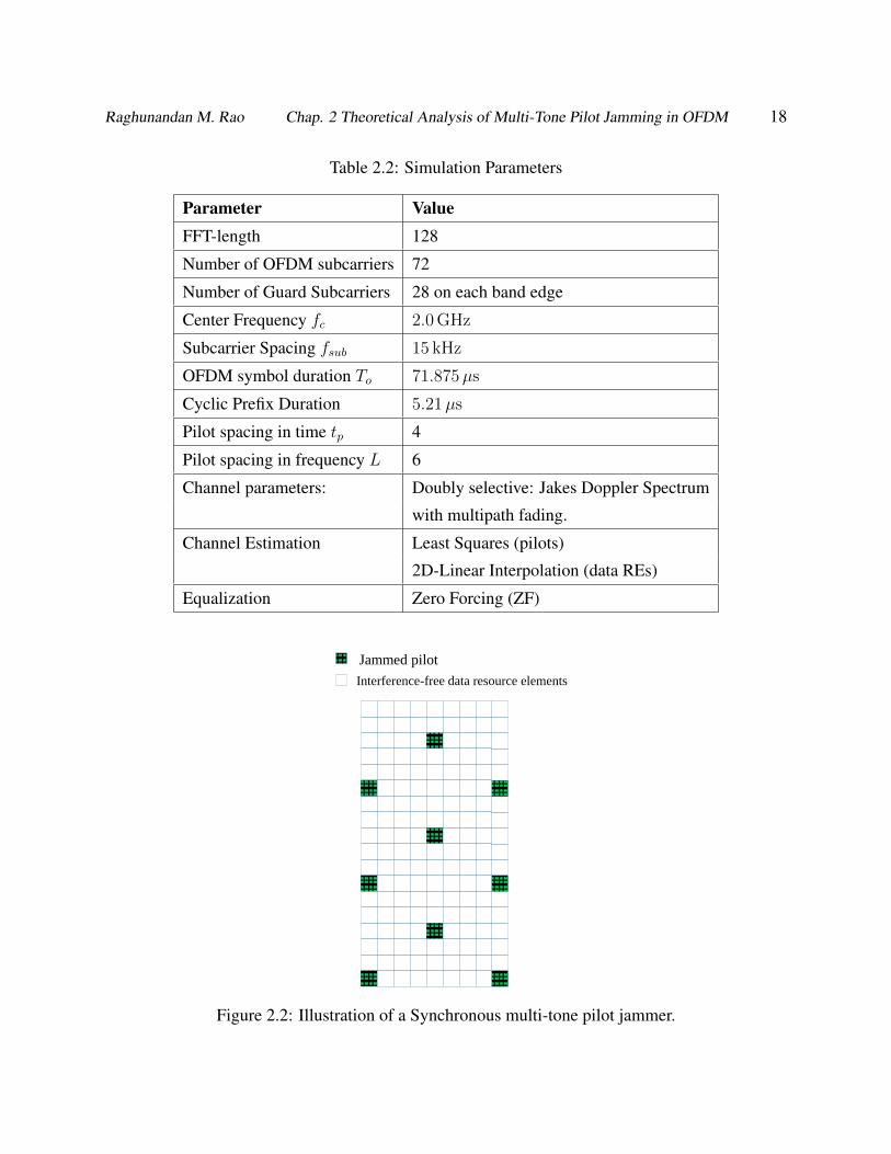
Table 2.2: Simulation Parameters
Parameter ValueFFT-length 128
Number of OFDM subcarriers 72
Number of Guard Subcarriers 28 on each band edge
Center Frequency fc 2.0 GHz
Subcarrier Spacing fsub 15 kHz
OFDM symbol duration To 71.875µs
Cyclic Prefix Duration 5.21µs
Pilot spacing in time tp 4
Pilot spacing in frequency L 6
Channel parameters: Doubly selective: Jakes Doppler Spectrum
with multipath fading.
Channel Estimation Least Squares (pilots)
2D-Linear Interpolation (data REs)
Equalization Zero Forcing (ZF)
Jammed pilot
Interference-free data resource elements
Figure 2.2: Illustration of a Synchronous multi-tone pilot jammer.
Raghunandan M. Rao Chap. 2 Theoretical Analysis of Multi-Tone Pilot Jamming in OFDM 19
2.4.3 Numerical Results
This subsection presents the validation of derived MSE expressions by numerical simulations. Ta-ble 2.2 summarizes the parameters of the OFDM system. Each channel is chosen to be doublyselective: Jakes Doppler Spectrum models the mobility effects in the channel, with Rayleigh fad-ing due to multipath modeled using a tapped delay-line model. The jammer is assumed to besynchronized with the target such that only pilot locations in the OFDM block are jammed, asshown in Figure 2.2.
We define the jammer-to-signal ratio per RE (JSR) to be the ratio between the received interfer-ence power and the received signal power on a target RE. Hence, JSR = 0 for interference-freeREs (non-pilot REs) and non-zero otherwise (pilots). The simulations consider equal power allo-cation on all resource elements of the target OFDM signal, and equal jammer power allocations onall targeted pilot locations.
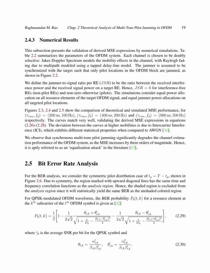
Figures 2.3, 2.4 and 2.5 show the comparison of theoretical and simulated MSE performance, for(τrms, fd) = (200 ns, 100 Hz), (τrms, fd) = (400 ns, 200 Hz) and (τrms, fd) = (900 ns, 500 Hz)respectively. The curves match very well, validating the derived MSE expressions in equations(2.26)-(2.28). The deviation between the curves at higher mobilities is due to Intercarrier Interfer-ence (ICI), which exhibits different statistical properties when compared to AWGN [31].
We observe that synchronous multi-tone pilot jamming significantly degrades the channel estima-tion performance of the OFDM system, as the MSE increases by three orders of magnitude. Hence,it is aptly referred to as an ‘equalization attack’ in the literature [12].
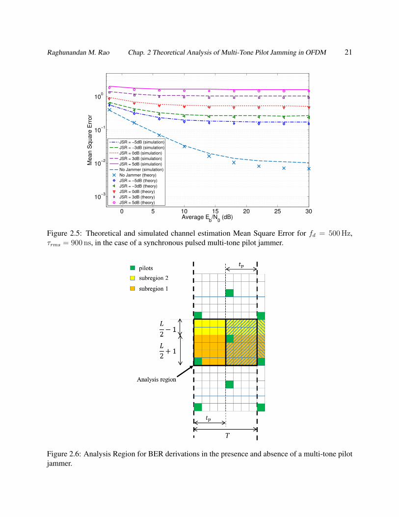
2.5 Bit Error Rate Analysis
For the BER analysis, we consider the symmetric pilot distribution case of tp = T − tp, shown inFigure 2.6. Due to symmetry, the region marked with upward diagonal lines has the same time andfrequency correlation functions as the analysis region. Hence, the shaded region is excluded fromthe analysis region since it will statistically yield the same BER as the unshaded colored region.
For QPSK-modulated OFDM waveforms, the BER probability Pb(t, k) for a resource element atthe kth subcarrier of the tth OFDM symbol is given as [32]
Pb(t, k) =1
2
[1− 1
2√
2
θt,k + θ′t,k√1 + 1
2γb− (θt,k−θ′t,k)2
2
− 1
2√
2
θt,k − θ′t,k√1 + 1
2γb− (θt,k+θ′t,k)2
2
], (2.29)
where γb is the average SNR per bit for the QPSK symbol and
θt,k =α′t,k
βt,kβ′t,k, θ′t,k =
α′′t,kβt,kβ′t,k
, (2.30)

Raghunandan M. Rao Chap. 2 Theoretical Analysis of Multi-Tone Pilot Jamming in OFDM 20
0 5 10 15 20 25 3010
−4
10−3
10−2
10−1
100
101
Average Eb/N
0 (dB)
Mean S
quare
Err
or
No Jammer (simulation)
JSR = −5dB (simulation)
JSR = −3dB (simulation)
JSR = 0dB (simulation)
JSR = 3dB (simulation)
JSR = 5dB (simulation)
JSR = 5dB (theory)
JSR = 3dB (theory)
JSR = 0dB (theory)
JSR = −3dB (theory)
JSR = −5dB (theory)
No Jammer (theory)
Figure 2.3: Theoretical and simulated channel estimation Mean Square Error for fd = 100 Hz,τrms = 200 ns, in the case of a synchronous pulsed multi-tone pilot jammer.
Average Eb/N
0 (dB)
0 5 10 15 20 25 30
Mean S
quare
Err
or
10-4
10-3
10-2
10-1
100
101
No Jammer (theory)
No Jammer (simulation)
JSR = -5dB (theory)
JSR = -3dB (theory)
JSR = 0dB (theory)
JSR = 3dB (theory)
JSR = 5dB (theory)
JSR = -5dB (simulation)
JSR = -3dB (simulation)
JSR = 0dB (simulation)
JSR =3dB (simulation)
JSR = 5dB (simulation)
Figure 2.4: Theoretical and simulated channel estimation Mean Square Error for fd = 200 Hz,τrms = 400 ns, in the case of a synchronous pulsed multi-tone pilot jammer.
Raghunandan M. Rao Chap. 2 Theoretical Analysis of Multi-Tone Pilot Jamming in OFDM 21
0 5 10 15 20 25 30
10−3
10−2
10−1
100
Average Eb/N
0 (dB)
Mean S
quare
Err
or
JSR = −5dB (simulation)
JSR = −3dB (simulation)
JSR = 0dB (simulation)
JSR = 3dB (simulation)
JSR = 5dB (simulation)
No Jammer (simulation)
No Jammer (theory)
JSR = −5dB (theory)
JSR = −3dB (theory)
JSR = 0dB (theory)
JSR = 3dB (theory)
JSR = 5dB (theory)
Figure 2.5: Theoretical and simulated channel estimation Mean Square Error for fd = 500 Hz,τrms = 900 ns, in the case of a synchronous pulsed multi-tone pilot jammer.
Figure 2.6: Analysis Region for BER derivations in the presence and absence of a multi-tone pilotjammer.
Raghunandan M. Rao Chap. 2 Theoretical Analysis of Multi-Tone Pilot Jamming in OFDM 22
β2t,k =
1
2E[|Hk[t]|2], β′
2t,k =
1
2E[|Hk[t]|2]
αt,k =1
2E[Hk[t]H
∗k [t]]
= α′t,k + jα′′t,k, (2.31)
where α′t,k, α′′t,k ∈ R. To derive the BER for the OFDM block with the diamond-shaped pilot
pattern, we substitute (2.11) and (2.12) in (2.29)-(2.31) for each resource element in the analysisregion and find the average. This is discussed in more detail in the next subsection.
2.5.1 BER in the Presence of a Synchronous Multi-Tone Pilot Jammer
In the presence of a multi-tone pilot jammer, the terms in (2.29) need to be calculated for sub-regions 1 and 2, shown in Figure 2.6. We will present the expressions for sub-region 1 in thissection; the corresponding expressions for sub-region 2 can be derived from those of sub-region 1by symmetry.
2.5.1.1 Lower REs of sub-region 1: 0 ≤ k ≤ L/2, 0 ≤ t < tp
We derive the BER expressions, with the same assumptions about the jammer as outlined in section2.4. Because the analysis region forms a basis of the 2D resource grid, we can simplify notationsby assuming m = 0 and n = 0 in (2.11) and (2.12), so that 0 ≤ k ≤ L/2 and 0 ≤ t < tp representthe equivalent ranges of subcarriers and time slots of sub-region 1. The corresponding channelestimate then becomes
HJk [t] = (1− η)
[(1− ζ)HJ
0 [0] + ζHJL [0]
]+ η[(1
2− ζ)HJ−L/2[tp] +
(1
2+ ζ)HJL/2[tp]
]. (2.32)
For βt,k we then obtain
β2t,k =
1
2E[|Hk[t]|2] = σ2
H/2. (2.33)
Note that Rf (0)Rt(0) = 1 as a result from (2.6)-(2.8) and
β′2t,k =
1
2E[|HJ
k [t]|2] =1
2[η2(1/2 + 2ζ2) + (1− η)2(1 + 2ζ2 − 2ζ)](σ2
H + σ2w + σ2
J)+
[(1− η)2(ζ − ζ2) + η2(1/4− ζ2)]<[Rf (L)]Rt(0) + η(1− η)[(1− ζ) + ζ(1/2 + ζ)]×<[Rf (L/2)]Rt(tp) + ηζ(1− η)(1/2− ζ)<[Rf (3L/2)]Rt(tp). (2.34)
Raghunandan M. Rao Chap. 2 Theoretical Analysis of Multi-Tone Pilot Jamming in OFDM 23
Similarly,
αt,k =1
2E[HJk [t]H∗k [t]
]=
1
2
(1− η)[(1− ζ)Rf (−k) + ζRf (L− k)]Rt(t) + η
[(1
2− ζ)Rf
(−L2− k)
+(1
2+ ζ)Rf
(L2− k)]Rt(tp − t)
. (2.35)
The BER of sub-region 1 REs Pb(t, k) can be found with (2.29) using (2.33)-(2.35).
2.5.1.2 Lower REs of sub-region 1: L/2 < k < L, 0 ≤ t < tp
The BER of sub-region 2 REs can be equivalently derived. Here, L/2 < k < L and 0 ≤ t < tp.We define k′ = k − L/2 and substitute it into equation (2.12) to obtain
HJk′ [t] = (1− η)
[(1
2− ζ ′
)HJ
0 [n] +(1
2+ ζ ′
)HJL [n]
]+ η[(1− ζ ′)HJ
L/2[tp] + ζ ′HJ3L/2[tp]
],
(2.36)
where ζ ′ , k′/L = ζ + 1/2. Noting the similarity of (2.36) with (2.32), and the fact that thetemporal correlation Rt(t) is an even function, we find the correlation terms of these resourceelements by substituting k′ = k − L/2 in (2.33)-(2.35). Therefore
αt,k′ = αt,k−L/2, βt,k′ = βt,k−L/2, β′t,k′ = β′t,k−L/2 (2.37)
can be found using (2.33)-(2.35) and used in (2.29) to find the BER Pb(t, k′) of a resource element
in sub-region 2.
2.5.1.3 Overall BER
The overall BER of the OFDM resource block with QPSK symbols in the presence of a multi-tonejammer P J
b,QPSK can finally be found by averaging the BER over all data resource elements in theanalysis region:
P Jb,QPSK =
1
L · tp − 1
[L−1∑
k=L/2+1
tp−1∑t=0
Pb(t, k − L/2) +
L/2∑k=0
tp−1∑t=0
Pb(t, k)− Pb(0, 0)
]. (2.38)
Note that pilot symbols do not contribute to the BER of the OFDM resource block and are thusexcluded for BER analysis.
Raghunandan M. Rao Chap. 2 Theoretical Analysis of Multi-Tone Pilot Jamming in OFDM 24
2.5.2 BER in the Absence of a Multi-Tone Pilot Jammer
In the absence of the multi-tone jammer we have σ2J = 0. Hence, only the term β′2t,k changes,
whereas the rest of the terms remain unchanged and can be computed in the same way as shown in(2.33)-(2.38).
This BER derivation can be extended to other modulation formats, such as QAM and higher or-der PSK [32], [33]. This is beyond the scope of the paper. Note, however that the correlationcoefficients αt,k, βt,k, β′t,k necessary for the BER calculations will remain the same for all thesemodulation formats.
2.5.3 Numerical Results
This subsection presents the validation of the accuracy of the derived BER expressions in thepresence and absence of a synchronous multi-tone jammer. Table 2.2 summarizes the parametersof the OFDM resource block. We define the JSR to be the ratio between the received interferencepower and the received signal power on a target RE.
Figures 2.7, 2.8 and 2.9 show the theoretical and simulated performance of QPSK-OFDM in thecase of a synchronous multi-tone pilot jammer, for (τrms, fd) = (200 ns, 100 Hz), (τrms, fd) =(400 ns, 200 Hz) and (τrms, fd) = (900 ns, 500 Hz) respectively. We have chosen these parametersin order to observe the accuracy of the derived expressions in (a) low frequency selectivity andmobility, (b) moderate frequency selectivity and mobility and (c) high frequency selectivity andmobility wireless channels. The theoretical and simulated BER curves closely match, thus vali-dating the analysis presented in section 2.5.1. Note that the high inter-carrier interference (ICI)[31] results in a slight mismatch between theoretical and simulated BER curves at higher values ofEb/N0, for higher fd values.
Thus, it is clear from these figures that a synchronous pilot jammer causes massive degradation inBER at higher values of Eb/N0 as well. Thus, it is a very effective attack that makes the jammermore energy-efficient. Once the BER increases beyond a value of 0.25, error correction codes ofthe system become ineffective. Thus, assuming that denial of service is caused for BER > 0.25,we see that the jammer can cause denial of service with a JSR of about 5 dB for all values ofEb/N0. This means that if the jammer perfectly localizes its power to the pilot locations of thetarget OFDM signal, it can cause denial of service with 2× 100.5/(6× 8) = 0.132 or ∼ 9 dB lesspower than the target signal for the parameters in Table 2.2. In general, if 1/η is the pilot density(number of pilots per OFDM block) and JSR (dB) the Jammer to Signal ratio of the synchronouspilot jammer, then the jammer requires a fraction ρ of the target OFDM signal power which canbe computed using
ρ =10
JSR(dB)10
η, (2.39)

Raghunandan M. Rao Chap. 2 Theoretical Analysis of Multi-Tone Pilot Jamming in OFDM 25
0 5 10 15 20 25 3010
−4
10−3
10−2
10−1
100
Average Eb/N
0 (dB)
Bit E
rro
r R
ate
JSR = −5dB (simulation)
JSR = −3dB (simulation)
JSR = 0dB (simulation)
JSR = 3dB (simulation)
JSR = 5dB (simulation)
No Jammer (simulation)
No Jammer (theory)
JSR = −5dB (theory)
JSR = −3dB (theory)
JSR = 0dB (theory)
JSR = 3dB (theory)
JSR = 5dB (theory)
Figure 2.7: Theoretical and simulated BER performance of QPSK-OFDM for fd = 100 Hz, τrms =200 ns,in the case of a synchronous pulsed multi-tone pilot jammer.
0 5 10 15 20 25 3010
−4
10−3
10−2
10−1
100
Average Eb/N
0 (dB)
Bit E
rro
r R
ate
No Jammer (simulation)
No Jammer (theory)
JSR = −5dB (simulation)
JSR = −3dB (simulation)
JSR = 0dB (simulation)
JSR = 3dB (simulation)
JSR = 5dB (simulation)
JSR = −5dB (theory)
JSR = −3dB (theory)
JSR = 0dB (theory)
JSR = 3dB (theory)
JSR = 5dB (theory)
Figure 2.8: Theoretical and simulated BER performance of QPSK-OFDM for fd = 200 Hz, τrms =400 ns,in the case of a synchronous pulsed multi-tone pilot jammer.

Raghunandan M. Rao Chap. 2 Theoretical Analysis of Multi-Tone Pilot Jamming in OFDM 26
0 5 10 15 20 25 3010
−3
10−2
10−1
100
Average Eb/N
0 (dB)
Bit E
rro
r R
ate
JSR = −5dB (simulation)JSR = −3dB (simulation)JSR = 0dB (simulation)JSR = 3dB (simulation)JSR = 5dB (simulation)JSR = 5dB (theory)JSR = 3dB (theory)JSR = 0dB (theory)JSR = −3dB (theory)JSR = −5dB (theory)No Jammer (simulation)No Jammer (theory)
Figure 2.9: Theoretical and simulated BER performance of QPSK-OFDM for fd = 500 Hz, τrms =900 ns, in the case of a synchronous pulsed multi-tone pilot jammer.
since the jammer transmits a power JSR (dB) higher than that of the victim signal at pilot lo-cations. Hence, ρ is analogous to the overall average Signal to Interference Ratio (SIR) at thereceiver, which depends on the sparsity of the pilots (1/η). The sparser the pilot density, thelower will be the value of ρ. Table 2.3 shows the relation between ρ and JSR for the simulationparameters in Table 2.2.
Table 2.3: Relationship between JSR (dB) and ρ.
JSR (dB) ρ∗ ρ∗ (dB)-5 0.0132 -18.8021-3 0.0209 -16.80210 0.0417 -13.80213 0.0831 -10.80215 0.1318 -8.8021
∗ assuming that the transmitter and jammer are located equidistant from the victim receiver. ρ will vary ifthe distances are different.

Raghunandan M. Rao Chap. 2 Theoretical Analysis of Multi-Tone Pilot Jamming in OFDM 27
2.6 Conclusions
In this chapter, we derived the expressions for the MSE of the linear interpolation-based channelestimation and the BER for QPSK-OFDM. We derived these expressions using the WSSUS chan-nel approximation, to model the system performance accurately, both in the presence and absenceof a multi-tone pilot jammer.
These derivations and its validation through numerical simulations demonstrate that synchronousmulti-tone pilot jamming is a very effective attack that can potentially cause DoS by transmittinga total of only about 10% of the power w.r.t. that of the OFDM transmitter in most cases. Thispower requirement will reduce for smaller pilot densities, making synchronous pilot jamming athreat to consider when the jammer is sophisticated. It is to be noted that reactive jamming wouldbe necessary in order to carry out these attacks in practice, since the jammer needs to know exactlywhen the target is receiving the downlink OFDM blocks.
The primary factor causing the performance degradation is corrupted channel estimates and hence,can be countered by first restoring the channel estimation performance in the presence of the pilotjammer. These approaches are the focus of the next chapter.

Chapter 3
Mitigation of Multi-Tone Pilot Jamming inSISO and MIMO-OFDM
3.1 Background
Multi-tone pilot jamming, unlike other types of interference, spreads the effect of localized inter-ference on the pilot REs to adjacent data REs by spoofing the channel estimation and equalization.Hence, degradation of performance to reach the point of Denial of Service (DoS), can be achievedwith lesser powers w.r.t. wideband barrage jamming when pilot signals are targeted. In orderto mitigate the multi-tone pilot jammer, firstly we would need to restore channel estimation per-formance in the presence of the jammer, which is the central goal of the work presented in thischapter.
For narrow-band interference on pilots, Han et al. [10] proposed a jammed pilot detection andexcision algorithm to mitigate the narrow-band jammer. However, a narrowband jammer will havea limited impact on the target’s throughput, because the system can still operate by not schedulingusers on the affected resource elements. To cause DoS, multiple pilots of the OFDM block willneed to be targeted.
Clancy [7, 8] analyzes pilot tone jamming and nulling and proposes pilot-tone randomization asa technique to evade the jammer. However, randomizing pilot tone locations leads to sub-optimalOFDM performance in the absence of a jammer [25] and requires higher layer protocols to commu-nicate the pilot patterns to legitimate users, which makes initial access to the cell a time-consumingprocedure.
Mitigation of pilot jamming in spatial multiplexing MIMO systems becomes challenging, as itwould require channel estimation between each transmit antenna - receive antenna pair. In tradi-tional beamforming systems, canceling out interference by null-steering or beam-steering usingmultiple antennas is possible because of the presence of a single spatial stream on all transmit
28
Raghunandan M. Rao Chap. 3 Mitigation of Multi-Tone Pilot Jamming in SISO and MIMO-OFDM 29
antennas [34, 35]. Mitigation of pilot jamming using beamforming algorithms is not possible inthe case of spatial multiplexing, because it involves transmission of independent streams of datafrom each antenna. Moreover it is even more challenging due to the fact that the pilot jammerdegrades Channel State Information (CSI) at the target, which are central to achieving capacityenhancements promised by spatial multiplexing.
Yan et al. [36] present a MIMO-based anti-jamming scheme utilizing MIMO interference cancel-lation and transmit precoding. They implement jammer cancellation using iterative jammer andtransmitter channel tracking in the case of a reactive jammer. This solution comes at the cost oflosing one spatial degree of freedom.
Sodagari et al. [37] propose randomizing pilot locations to mitigate pilot jamming in MIMO sce-narios, in a similar manner as proposed in [7, 8]. Cole et al. [13] propose a new method of design-ing a MIMO antijamming communications system called ‘Spatial Hiding Antijamming’, whichrelies on making the transmit precoding vector orthogonal to the jammer channel matrix. The useof transmit precoding methods to mitigate the multi-tone pilot jammer is difficult to implementfor broadcast pilot jamming, where each affected user will potentially need a different precodingmatrix, in addition to perfect CSI to mitigate the pilot jammer. Most current wireless standardsallow for choice of precoding matrices from a finite-sized codebook.
The aim of this chapter is to present and analyze methods that can restore channel estimationperformance in the presence of a multi-tone pilot jammer for both SISO- and MIMO-OFDM case.In our proposed jammer mitigation algorithms for a SISO-OFDM system, we seek to preserve theoptimal pilot configuration that minimizes the MSE [25]. For MIMO-OFDM systems, our focusis on methods that can achieve full rank spatial multiplexing in the presence of the jammer. Weshow that it is possible to mitigate a power-constrained multi-tone pilot jammer with little to nointervention from the base station.
Section 3.2 describes the most common jamming strategies, and outlines our definition of a power-constrained pilot jammer. Section 3.3 provides a brief overview about the detection of pilot jam-ming. Section 3.4 presents our proposed algorithms to mitigate the pilot jammer, its performance,and highlights the applicability of these methods in LTE. Section 3.5 presents a brief overviewof spatial multiplexing in MIMO-OFDM, the jammer model, an approximate channel estimationalgorithm to mitigate the power-constrained pilot jammer and its performance results. Section 3.6concludes the chapter with a summary of the main results.
3.2 Types of Multi-Tone Pilot Jammers
The multitone pilot jammer can have power allocation strategies with varying levels of sophistica-tion. The jammer can transmit continuously, or can allocate power based on its knowledge of thedownlink signal [38]. In this work, we consider two broad classes of jammer strategies:
1. Continuous Asynchronous Jammer: Requires knowledge of the pilot subcarrier indices only.

Raghunandan M. Rao Chap. 3 Mitigation of Multi-Tone Pilot Jamming in SISO and MIMO-OFDM 30
Since it is an asynchronous continuous transmission, the jammer has less complexity, butlower energy efficiency.
2. Pulsed Synchronous Jammer: Requires tight synchronization with the target’s receiver, butprovides high energy efficiency at the cost of jammer complexity.
As discussed before, we consider power-constrained multi-tone pilot jammers in this work. Theaim of such a jammer is to maximize its power efficiency while being constrained to the strategy itchooses to use.
Definition 3.1. A Power-constrained jammer
1. Transmits on all possible pilot subcarriers continuously at a lower data rate than the targetsignal, in the case of an asynchronous jammer.
2. Transmits only on pilot locations of the OFDM grid, in the case of a synchronous jammer.This is straightforward for SISO-OFDM, but it becomes slightly complicated for MIMO-OFDM where some pilot locations might be adjacent to each other. In this case, the jammerwould need to transmit its modulation symbols at a lower data rate as compared to the targetOFDM signal.
The reasoning for such a definition for the asynchronous jammer is as follows. If the asynchronousjammer intends to be power efficient, it needs to make sure that all of it power is aligned with pilotsubcarriers. A potential issue with modulation symbols is spectral leakage of power into adjacentsubcarriers. Spectral leakage can be minimized if the jammer has a lower symbol rate on eachtargeted subcarrier, than the target OFDM signal [39]. In addition to pulse shape and modulationof jammer data symbols, jammer mobility results in inter-carrier interference at the target receiver,as a result of shift in jammer spectra w.r.t. the pilot subcarrier due to Doppler. Hence, strong powerlocalization on the pilot locations in a fast fading wireless channel is possible with lower data ratesfor the jammer digital modulated signal w.r.t. the target OFDM symbol.
Traditionally, narrowband interference is mitigated either by Interference Cancellation (IC) or jam-mer evasion strategies. Since multi-tone pilot jamming in OFDM consists of multiple narrowbandsignals, we propose two strategies to mitigate it for SISO scenarios: resource element blankingwith interference cancellation and jammer evasion by cyclic shifting of pilot locations.
3.3 Detection of Pilot Jamming
Before mitigating pilot jamming, it is necessary to detect that the jamming has occurred. Thereare various types of detectors with varying complexities from simple energy detection [10] tosophisticated interference detection with modulation classification algorithms [40]. The methodspresented in this chapter result in little to no degradation in the case of a false negative during the
Raghunandan M. Rao Chap. 3 Mitigation of Multi-Tone Pilot Jamming in SISO and MIMO-OFDM 31
jammer detection process. The rest of this chapter assumes that presence of the jammer on pilottones is detected using any of the methods available in the literature. The focus of this chapter ismore on interference-aware pilot jamming mitigation, rather than the detection of pilot jammingitself.
When it comes to wireless standards, a lot of channel quality parameters can be utilized to detectthe presence of the pilot jammer. For the 3GPP LTE standard, these parameters include ChannelQuality Indicator (CQI), Reference Signal Received Power (RSRP), Reference Signal ReceivedQuality (RSRQ) and Received Signal Strength Indicator (RSSI) [41]. A description of few ofthese parameters will be discussed with more details in chapter 4.
3.4 Anti-Jamming for SISO-OFDM Systems
3.4.1 Resource Element Blanking with Interference Cancellation
Asynchronous multi-tone pilot jamming is simple to implement and would be suitable for jammersthat do not have very tight power constraints. For this type of jammer we propose resource elementblanking with interference cancellation as illustrated in Figure 3.1.
Suppose that a pilot symbol is carried over the lth subcarrier during time interval n and that thelth subcarrier is jammed over all OFDM symbols. The channel estimate Hl[n] based on resourceelement blanking and interference cancellation can be obtained as
Hl[n] = Hl[n] +H ′l [n]Jl[n]−H ′l [n+ 1]Jl[n+ 1]
Pl[n]
+(wl[n]− wl[n+ 1])
Pl[n]. (3.1)
The underlying assumption here is that the channels and the jamming signal remain constant overthe two consecutive OFDM symbols; that is, H ′l [n] ≈ H ′l [n + 1] and Jl[n] = Jl[n + 1] due todefinition 3.1. In practice, the channel estimation and BER performance depends on the relativemobility between the jammer and the target receiver. Higher mobility leads to lower temporalcorrelation, thus resulting in slightly degraded performance of the proposed approach. In eithercase, because (wl[n] − wl[n + 1]) ∼ CN (0, 2σ2
w), this method enhances the additive complexGaussian noise component on the pilot and reduces its average SNR per bit (Eb/N0) by at least3 dB. Implementation of this approach in the 3GPP LTE standard is simple, because of the in-built blanking of REs adjacent to reference signal locations on all antenna ports to support MIMOoperation [42].

Raghunandan M. Rao Chap. 3 Mitigation of Multi-Tone Pilot Jamming in SISO and MIMO-OFDM 32
Figure 3.1: Mitigation of asynchronous multi-tone pilot jamming by resource element blankingwith interference cancellation.
Figure 3.2: Mitigation of synchronous multi-tone pilot jamming by cyclic frequency shifting ofpilot locations.
Raghunandan M. Rao Chap. 3 Mitigation of Multi-Tone Pilot Jamming in SISO and MIMO-OFDM 33
3.4.2 Cyclic Frequency Shifting of Pilot Locations
Interference cancellation is impossible without the knowledge of the jammer characteristics. If thejammer perfectly synchronizes with the receiver, and localizes its power on the pilot locations ofthe OFDM grid, tracking the jammer signal for cancellation becomes very hard in practice. In thiscase, the receiver can coordinate with the transmitter to cyclically shift all the pilot locations byone or more subcarriers to evade the jamming signal, as illustrated in Figure 3.2.
This feature is present in the 3GPP LTE/LTE-A standard where a cell-specific frequency shift isapplied to the pilot locations based on a cell parameter, called the physical cell identity (PCI) ofthe network [42]. This mitigation strategy can be used with dynamic PCI planning approaches[43], to make provisions in the protocol for future releases of LTE to protect it against targetedinterference. The advantage of this approach is that it would maintain optimal channel estimationperformance due to equal pilot spacing in time and frequency [25], even in the presence of a multi-tone pilot jammer. This method is more suitable for cases where it is not feasible to use interferencecancellation procedures to mitigate the pilot interference. However, the network implications ofdynamic shifting of pilot locations in a cell need more analysis for network-wise solutions.
3.4.3 Numerical Results
Here we analyze the effectiveness of the proposed mitigation strategies. The simulation parametersare summarized in Table 2.2. We assume that the channels between the base station to the receiver,and jammer to the receiver have the same Doppler and rms delay spreads fd and τrms. We comparethe of the channel estimation and the BER performance in the following scenarios:
1. Synchronous and asynchronous multi-tone pilot jamming with no mitigation,
2. Asynchronous multi-tone pilot jamming with resource element blanking and jammer can-cellation (JC),
3. Synchronous multi-tone pilot jamming with cyclic shifting of pilot locations,
4. No jammer.
We assume that the power allocated to pilot REs and data REs in the OFDM signal are the same. Itis important to note that even though the jamming duration varies for an asynchronous pilot jammerw.r.t. a synchronous pilot jammer, we are interested in the interference power on the pilots. Hencewe use the following definition of JSR for comparison between the different jammer strategies.
Definition 3.2. Jammer to Signal Ratio (JSR) is defined as
1. The ratio of jammer power to signal power for each jammed pilot RE in the case of a syn-chronous multi-tone pilot jammer.
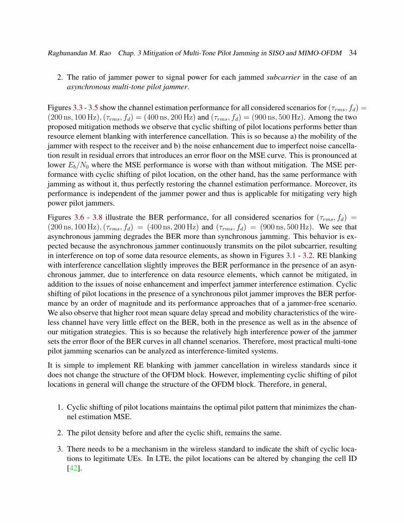
Raghunandan M. Rao Chap. 3 Mitigation of Multi-Tone Pilot Jamming in SISO and MIMO-OFDM 34
2. The ratio of jammer power to signal power for each jammed subcarrier in the case of anasynchronous multi-tone pilot jammer.
Figures 3.3 - 3.5 show the channel estimation performance for all considered scenarios for (τrms, fd) =(200 ns, 100 Hz), (τrms, fd) = (400 ns, 200 Hz) and (τrms, fd) = (900 ns, 500 Hz). Among the twoproposed mitigation methods we observe that cyclic shifting of pilot locations performs better thanresource element blanking with interference cancellation. This is so because a) the mobility of thejammer with respect to the receiver and b) the noise enhancement due to imperfect noise cancella-tion result in residual errors that introduces an error floor on the MSE curve. This is pronounced atlower Eb/N0 where the MSE performance is worse with than without mitigation. The MSE per-formance with cyclic shifting of pilot location, on the other hand, has the same performance withjamming as without it, thus perfectly restoring the channel estimation performance. Moreover, itsperformance is independent of the jammer power and thus is applicable for mitigating very highpower pilot jammers.
Figures 3.6 - 3.8 illustrate the BER performance, for all considered scenarios for (τrms, fd) =(200 ns, 100 Hz), (τrms, fd) = (400 ns, 200 Hz) and (τrms, fd) = (900 ns, 500 Hz). We see thatasynchronous jamming degrades the BER more than synchronous jamming. This behavior is ex-pected because the asynchronous jammer continuously transmits on the pilot subcarrier, resultingin interference on top of some data resource elements, as shown in Figures 3.1 - 3.2. RE blankingwith interference cancellation slightly improves the BER performance in the presence of an asyn-chronous jammer, due to interference on data resource elements, which cannot be mitigated, inaddition to the issues of noise enhancement and imperfect jammer interference estimation. Cyclicshifting of pilot locations in the presence of a synchronous pilot jammer improves the BER perfor-mance by an order of magnitude and its performance approaches that of a jammer-free scenario.We also observe that higher root mean square delay spread and mobility characteristics of the wire-less channel have very little effect on the BER, both in the presence as well as in the absence ofour mitigation strategies. This is so because the relatively high interference power of the jammersets the error floor of the BER curves in all channel scenarios. Therefore, most practical multi-tonepilot jamming scenarios can be analyzed as interference-limited systems.
It is simple to implement RE blanking with jammer cancellation in wireless standards since itdoes not change the structure of the OFDM block. However, implementing cyclic shifting of pilotlocations in general will change the structure of the OFDM block. Therefore, in general,
1. Cyclic shifting of pilot locations maintains the optimal pilot pattern that minimizes the chan-nel estimation MSE.
2. The pilot density before and after the cyclic shift, remains the same.
3. There needs to be a mechanism in the wireless standard to indicate the shift of cyclic loca-tions to legitimate UEs. In LTE, the pilot locations can be altered by changing the cell ID[42].

Raghunandan M. Rao Chap. 3 Mitigation of Multi-Tone Pilot Jamming in SISO and MIMO-OFDM 35
4. In LTE, the cell IDs are chosen in order to minimize the interference on pilots of once cellfrom the others [1]. Hence, strategies such as dynamic PCI planning will be necessary tominimize the interference on the pilot signals of all surrounding cells [43].
The proposed mitigation methods help restoring the channel estimation performance in the pres-ence of a multi-tone pilot jammer. However, neither of these mitigation techniques can protect datathat is being jammed when the jammer transmits continuously. In this case, additional strategies,such as adaptive modulation and coding, resource blanking, adaptive bit loading and smart resourceallocation, are needed to attain low BER values. These techniques alone would not be effective ifthe pilots are corrupted and cannot be restored in the first place. The protection of pilots is thusof most importance, because if pilots are compromised, the channel estimation and equalizationfor the data-carrying resource elements would be inaccurate resulting in low performance [7], [8].Hence, this needs to be seriously addressed for protecting user equipment (UEs) and ensuring thatfuture systems will be more robust.
3.5 Spatial Multiplexing with MIMO-OFDM in the Presenceof Multi-Tone Pilot Jamming
3.5.1 Motivation
In the last few decades, wireless communication systems have utilized multiple antennas to ac-complish either of the following [44]:
1. Enhance the SNR using antenna diversity.
2. Improve the SINR using a combination of beamforming, beam steering and null steering.
3. Scale the throughput linearly with the number of antennas, using MIMO spatial multiplex-ing.
Traditionally, interference cancellation has been accomplished by null steering or beam steering[34, 35], which is applicable for multiple antennas tramsmitting a single spatial stream. But inthe current market environment and the road towards 5G, wireless carriers are more interested inincreasing wireless capacity rather than signal quality exclusively. This is why transmission ofmultiple data streams using spatial multiplexing has been used to enhance the throughput of thecurrent 4G technologies [1], as compared to its predecessors. It is expected to remain central tothe design of the future 5G wireless networks [45]. Moreover, it is inefficient to give up spatialdegrees of freedom to cancel out multi-tone pilot jamming, because the interference is sparse andtargeted on specific subcarriers/REs of the OFDM blocks.
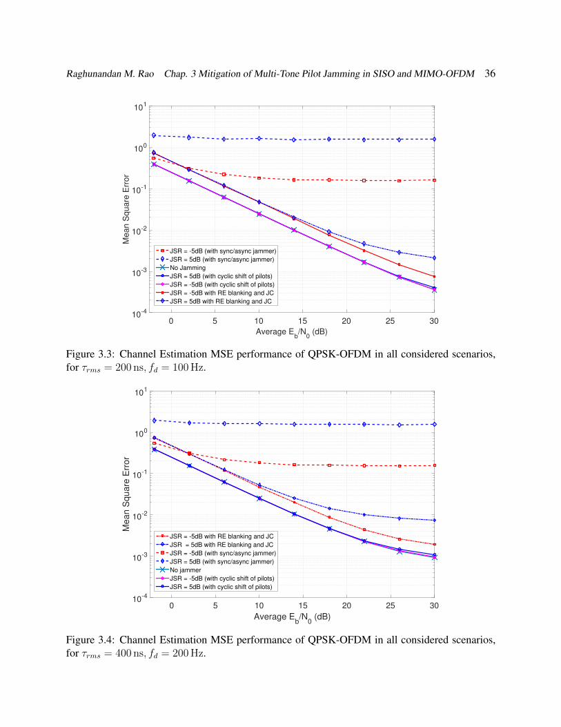
Raghunandan M. Rao Chap. 3 Mitigation of Multi-Tone Pilot Jamming in SISO and MIMO-OFDM 36
Average Eb/N
0 (dB)
0 5 10 15 20 25 30
Me
an
Sq
ua
re E
rro
r
10-4
10-3
10-2
10-1
100
101
JSR = -5dB (with sync/async jammer)
JSR = 5dB (with sync/async jammer)
No Jamming
JSR = 5dB (with cyclic shift of pilots)
JSR = -5dB (with cyclic shift of pilots)
JSR = -5dB with RE blanking and JC
JSR = 5dB with RE blanking and JC
Figure 3.3: Channel Estimation MSE performance of QPSK-OFDM in all considered scenarios,for τrms = 200 ns, fd = 100 Hz.
Average Eb/N
0 (dB)
0 5 10 15 20 25 30
Mean S
quare
Err
or
10-4
10-3
10-2
10-1
100
101
JSR = -5dB with RE blanking and JC
JSR = 5dB with RE blanking and JC
JSR = -5dB (with sync/async jammer)
JSR = 5dB (with sync/async jammer)
No jammer
JSR = -5dB (with cyclic shift of pilots)
JSR = 5dB (with cyclic shift of pilots)
Figure 3.4: Channel Estimation MSE performance of QPSK-OFDM in all considered scenarios,for τrms = 400 ns, fd = 200 Hz.

Raghunandan M. Rao Chap. 3 Mitigation of Multi-Tone Pilot Jamming in SISO and MIMO-OFDM 37
Average Eb/N
0 (dB)
0 5 10 15 20 25 30
Me
an
Sq
ua
re E
rro
r
10-3
10-2
10-1
100
101
JSR = -5dB (with sync/async jammer)
JSR = 5dB (with sync/async jammer)
JSR = -5dB with RE blanking and JC
JSR = 5dB with RE blanking and JC
No Jamming
JSR = 5dB (with cyclic shift of pilots)
JSR = -5dB (with cyclic shift of pilots)
Figure 3.5: Channel Estimation MSE performance of QPSK-OFDM in all considered scenarios,for τrms = 900 ns, fd = 500 Hz.
Average Eb/N
0 (dB)
0 5 10 15 20 25 30
Bit E
rro
r R
ate
10-4
10-3
10-2
10-1
100
JSR = -5dB (sync jammer)
JSR = 5dB (sync jammer)
JSR = -5dB (async jammer)
JSR = 5dB (async jammer)
JSR = -5dB with RE blanking and JC
JSR = 5dB with RE blanking and JC
JSR = -5dB (with cyclic freq shift of pilots)
JSR = 5dB (with cyclic freq shift of pilots)
No Jamming
Figure 3.6: Bit Error rate performance of QPSK-OFDM in all considered scenarios, for τrms =200 ns, fd = 100 Hz.
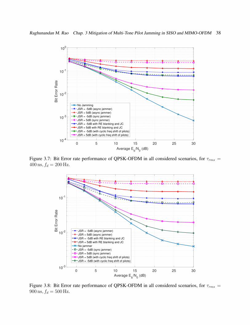
Raghunandan M. Rao Chap. 3 Mitigation of Multi-Tone Pilot Jamming in SISO and MIMO-OFDM 38
Average Eb/N
0 (dB)
0 5 10 15 20 25 30
Bit E
rror
Rate
10-4
10-3
10-2
10-1
100
No Jamming
JSR = -5dB (async jammer)
JSR = 5dB (async jammer)
JSR = -5dB (sync jammer)
JSR = 5dB (sync jammer)
JSR = -5dB with RE blanking and JC
JSR = 5dB with RE blanking and JC
JSR = -5dB (with cyclic freq shift of pilots)
JSR = 5dB (with cyclic freq shift of pilots)
Figure 3.7: Bit Error rate performance of QPSK-OFDM in all considered scenarios, for τrms =400 ns, fd = 200 Hz.
Average Eb/N
0 (dB)
0 5 10 15 20 25 30
Bit E
rro
r R
ate
10-3
10-2
10-1
JSR = -5dB (async jammer)
JSR = 5dB (async jammer)
JSR = -5dB with RE blanking and JC
JSR = 5dB with RE blanking and JC
No jammer
JSR = -5dB (sync jammer)
JSR = 5dB (sync jammer)
JSR = 5dB (with cyclic freq shift of pilots)
JSR = -5dB (with cyclic freq shift of pilots)
Figure 3.8: Bit Error rate performance of QPSK-OFDM in all considered scenarios, for τrms =900 ns, fd = 500 Hz.

Raghunandan M. Rao Chap. 3 Mitigation of Multi-Tone Pilot Jamming in SISO and MIMO-OFDM 39
In the areas of MU-MIMO, techniques like precoding have been developed that can null multi-user interference. The authors of [13] have devised a method called Spatial Hiding Precoding,where transmit precoding vectors are chosen orthogonal to the channel vector of the jammer (witha single transmit antenna). However, this assumes perfect knowledge of the channels betweenthe jammer and the receiver, and between the transmitter and receiver, which is hard to obtainif a) the jammer is persistently corrupting channel estimates, and b) either of the channels fadesfast in a high mobility scenario. In addition, in the case of broadcast pilot jamming the transmitprecoding vector will drastically vary for each and every user, which makes its implementationvery challenging.
In this section, we show that a power-constrained multi-tone pilot jammer can be mitigated to someextent at each user independently of the other users without any assistance from the base station.
3.5.2 Channel Equalization in MIMO-OFDM
MIMO-OFDM systems use similar pilot-assisted methods as SISO systems to estimate the wirelesschannel. For Nt × Nr MIMO system, with Nt and Nr being the number of transmit and receiveantennas respectively, equalization would require Nt different pilot patterns, one for each transmitantenna. Prior work [25] has shown equal pilot spacing in time and frequency to be optimal inthe MMSE sense. Moreover, diamond-shaped pilots are used in the current 3GPP LTE/LTE-Astandard for supporting MIMO operation. We have used a similar pilot pattern for our analysis,which is shown for a 4 × 4 MIMO-OFDM block in Figure 3.9. The RE nulls are present in theOFDM block of each antenna port to ensure that there is no interference due to antenna j on thepilot locations of transmit antenna port i, for i 6= j and i, j ≤ Nt. We consider least squares (LS)with linear interpolation as the channel estimator, with a zero forcing (ZF) equalizer [44] at thereceiver.
Channel estimation is performed using the pilots from allNt transmit antennas, using the algorithmpresented in equations (2.9) - (2.12) of Section 2.3. After removing the cyclic prefix at the receiverand performing channel estimation, let H(ji)
k [n] denote the frequency domain channel estimatefor the channel between the ith transmit and jth receive antenna for the kth subcarrier of the nth
OFDM symbol. The corresponding frequency domain channel coefficient is denoted by H(ji)k [n].
The most important notations are summarized in Table 3.1
The overall MIMO-OFDM system can be represented by
Yk[n] = Hk[n]Xk[n] + Wk[n], (3.2)
where Yk[n] is a Nr × 1 vector denoting the received data vector, given by
Yk[n] =[Y
(1)k [n] Y
(2)k [n] · · · Y
(Nr)k [n]
]T. (3.3)
The superscript (.)(j) refers to the index of the receive antenna and [.]T the matrix transpose, for

Raghunandan M. Rao Chap. 3 Mitigation of Multi-Tone Pilot Jamming in SISO and MIMO-OFDM 40
Table 3.1: Important Symbols and Notation
Variable Domain† DescriptionNt Z+ Number of transmit antennasNr Z+ Number of receive antennas
Yk[n] CNr×1 Received data vector at the kth subcarrier of the nth OFDM symbolY
(j)k [n] C Received data at the jth receive antenna on the kth subcarrier of the nth
OFDM symbol, for 1 ≤ j ≤ Nr
Xk[n] MNt×1 Transmitted data vector at the kth subcarrier of the nth OFDM symbolX
(i)k [n] M Transmitted data at the ith transmit antenna on the kth subcarrier of the
nth OFDM symbol, for 1 ≤ i ≤ Nt
Hk[n] CNr×Nt Channel matrix at the kth subcarrier of the nth OFDM symbolHk[n] CNr×Nt Estimated channel matrix at the kth subcarrier of the nth OFDM symbolH
(ji)k [n] C Estimated channel between the ith transmit and the jth receive antenna
at the kth subcarrier of the nth OFDM symbolWk[n] CNr×1 complex AWGN vector at the kth subcarrier of the nth OFDM symbolσ2w R Noise power
W(j)k [n] C complex AWGN at the jth receive antenna on the kth subcarrier of
the nth OFDM symbol. W (j)k [n] ∼ N (0, σ2
w) for 1 ≤ j ≤ Nr.H
(j)′
k [n] C Channel coefficient between the jammer and the jth receive antenna ofthe target receiver on the kth subcarrier of the nth OFDM symbol,for 1 ≤ j ≤ Nr.
Jk[n] C Transmitted jammer symbol on the kth subcarrier of the nth OFDMsymbol.
† Z+ denotes the set of all positive integers, Cm×n denotes the set containing all possible m × n complexmatrices, Rm×n denotes the set containing all possible m× n matrices with real elements, MNt×1 denotesa Nt × 1 column vector containing modulation alphabets (we assume QPSK modulation in this chapter).
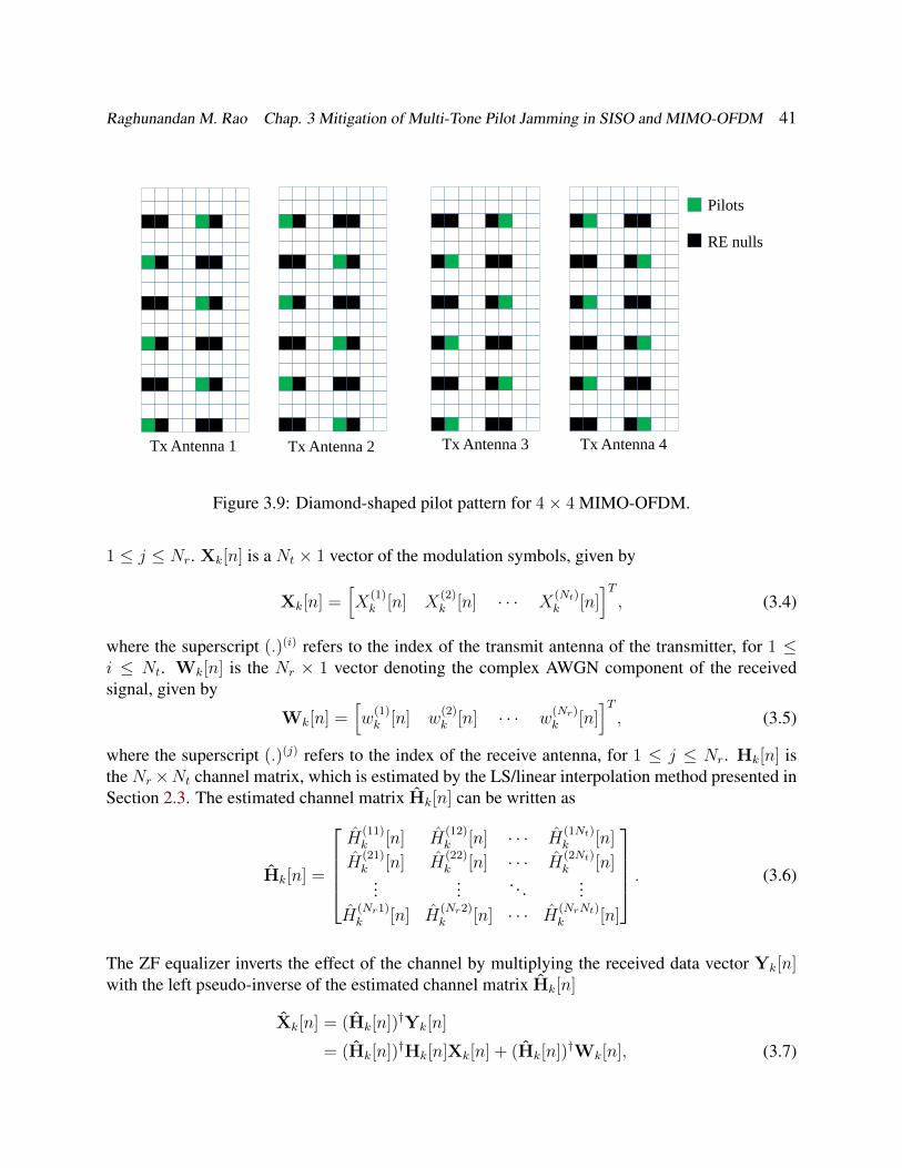
Raghunandan M. Rao Chap. 3 Mitigation of Multi-Tone Pilot Jamming in SISO and MIMO-OFDM 41
Tx Antenna 1 Tx Antenna 2 Tx Antenna 3 Tx Antenna 4
Pilots
RE nulls
Figure 3.9: Diamond-shaped pilot pattern for 4× 4 MIMO-OFDM.
1 ≤ j ≤ Nr. Xk[n] is a Nt × 1 vector of the modulation symbols, given by
Xk[n] =[X
(1)k [n] X
(2)k [n] · · · X
(Nt)k [n]
]T, (3.4)
where the superscript (.)(i) refers to the index of the transmit antenna of the transmitter, for 1 ≤i ≤ Nt. Wk[n] is the Nr × 1 vector denoting the complex AWGN component of the receivedsignal, given by
Wk[n] =[w
(1)k [n] w
(2)k [n] · · · w
(Nr)k [n]
]T, (3.5)
where the superscript (.)(j) refers to the index of the receive antenna, for 1 ≤ j ≤ Nr. Hk[n] isthe Nr×Nt channel matrix, which is estimated by the LS/linear interpolation method presented inSection 2.3. The estimated channel matrix Hk[n] can be written as
Hk[n] =
H
(11)k [n] H
(12)k [n] · · · H
(1Nt)k [n]
H(21)k [n] H
(22)k [n] · · · H
(2Nt)k [n]
...... . . . ...
H(Nr1)k [n] H
(Nr2)k [n] · · · H
(NrNt)k [n]
. (3.6)
The ZF equalizer inverts the effect of the channel by multiplying the received data vector Yk[n]with the left pseudo-inverse of the estimated channel matrix Hk[n]
Xk[n] = (Hk[n])†Yk[n]
= (Hk[n])†Hk[n]Xk[n] + (Hk[n])†Wk[n], (3.7)

Raghunandan M. Rao Chap. 3 Mitigation of Multi-Tone Pilot Jamming in SISO and MIMO-OFDM 42
where Xk[n] is a Nt × 1 vector denoting the estimated transmitted symbols. The pseudo-inversematrix (Hk[n])† is given by
(Hk[n])† = [(Hk[n])HHk[n]]−1(Hk[n])H , (3.8)
where (.)H denotes the Hermitian-transpose operation. Equation (3.7) is applied for 0 ≤ k ≤N − 1, 1 ≤ i ≤ Nt, 1 ≤ j ≤ Nr and all OFDM symbol indices n. Further detection and decodingprocesses are carried out to recover Nt distinct spatial data streams from the transmitter.
3.5.3 Multi-Tone Pilot Jamming Model for MIMO-OFDM
At the receiver, the OFDM blocks on each antenna have the pattern shown in Figure 3.10. Inthe rest of this section, we consider a synchronous multi-tone pilot jammer with a single transmitantenna, which transmits only on the time-frequency locations of the MIMO-OFDM grid whereall the pilots are located. As evident from Figure 3.9, the same pilot pattern will be used by allthe Nr receive antennas for channel estimation. Hence, the jammer interferes with all the receiveantennas by targeting the pilot locations of all Nt transmit antennas. We assume that the jammer isunaware of the channel between the itself and the receiver, in which case equal power allocation isoptimal to degrade the Bit Error Rate at the receiver [46]. This strategy is applicable in broadcastpilot jamming where the jammer aims to interfere with all receivers of the cell.
In order to minimize spectral leakage of its power, it is beneficial to have a lower symbol rate oneach subcarrier than the target OFDM signal, as explained in Definition 3.1. The jammer’s trans-mitted symbols across different subcarriers can vary, even though it has been shown that transmit-ting the same sequence across all pilots causes more damage to the receiver post-equalizationSINR [21]. This can also be inferred from the BER and MSE analysis presented in Chapter2. If the jamming signal on one pilot location is correlated with that on every other pilot, thenE[Jl[n]J∗k [m]
]> 0 for n 6= m or k 6= l, which results in higher MSE and BER values.
To summarize, the main assumptions about the pilot jammer are
1. The jammer has a single transmit antenna.
2. The jammer transmits only on the exact time-frequency locations of the target OFDM blocks.
3. Symbols transmitted by the jammer remain constant over adjacent OFDM symbols on thesame subcarrier.
4. The jammer transmits equal power on all the pilot locations.
We now present a channel estimation algorithm to mitigate this jammer. This algorithm doesnot sacrifice full rank spatial multiplexing operation even in the presence of a power-constrainedsynchronous multi-tone pilot jammer.
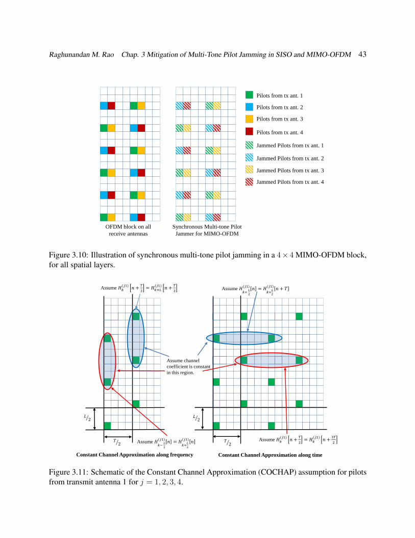
Raghunandan M. Rao Chap. 3 Mitigation of Multi-Tone Pilot Jamming in SISO and MIMO-OFDM 43
Pilots from tx ant. 1
Pilots from tx ant. 2
Pilots from tx ant. 3
Pilots from tx ant. 4
OFDM block on all
receive antennas
Synchronous Multi-tone Pilot
Jammer for MIMO-OFDM
Jammed Pilots from tx ant. 1
Jammed Pilots from tx ant. 2
Jammed Pilots from tx ant. 3
Jammed Pilots from tx ant. 4
Figure 3.10: Illustration of synchronous multi-tone pilot jamming in a 4× 4 MIMO-OFDM block,for all spatial layers.
Assume channel
coefficient is constant
in this region.
Constant Channel Approximation along frequency Constant Channel Approximation along time
Assume 𝐻𝑘(𝑗1)
𝑛 +𝑇
2= 𝐻𝑘+𝐿
(𝑗1)𝑛 +
𝑇
2
Assume 𝐻𝑘−
𝐿
2
(𝑗1)𝑛 = 𝐻
𝑘+𝐿
2
(𝑗1)𝑛
Assume 𝐻𝑘+
𝐿
2
(𝑗1)𝑛 = 𝐻
𝑘+𝐿
2
(𝑗1)𝑛 + 𝑇
Assume 𝐻𝑘(𝑗1)
𝑛 +𝑇
2= 𝐻𝑘
(𝑗1)𝑛 +
3𝑇
2 𝑇 2 𝑇 2
𝐿 2 𝐿 2
Figure 3.11: Schematic of the Constant Channel Approximation (COCHAP) assumption for pilotsfrom transmit antenna 1 for j = 1, 2, 3, 4.
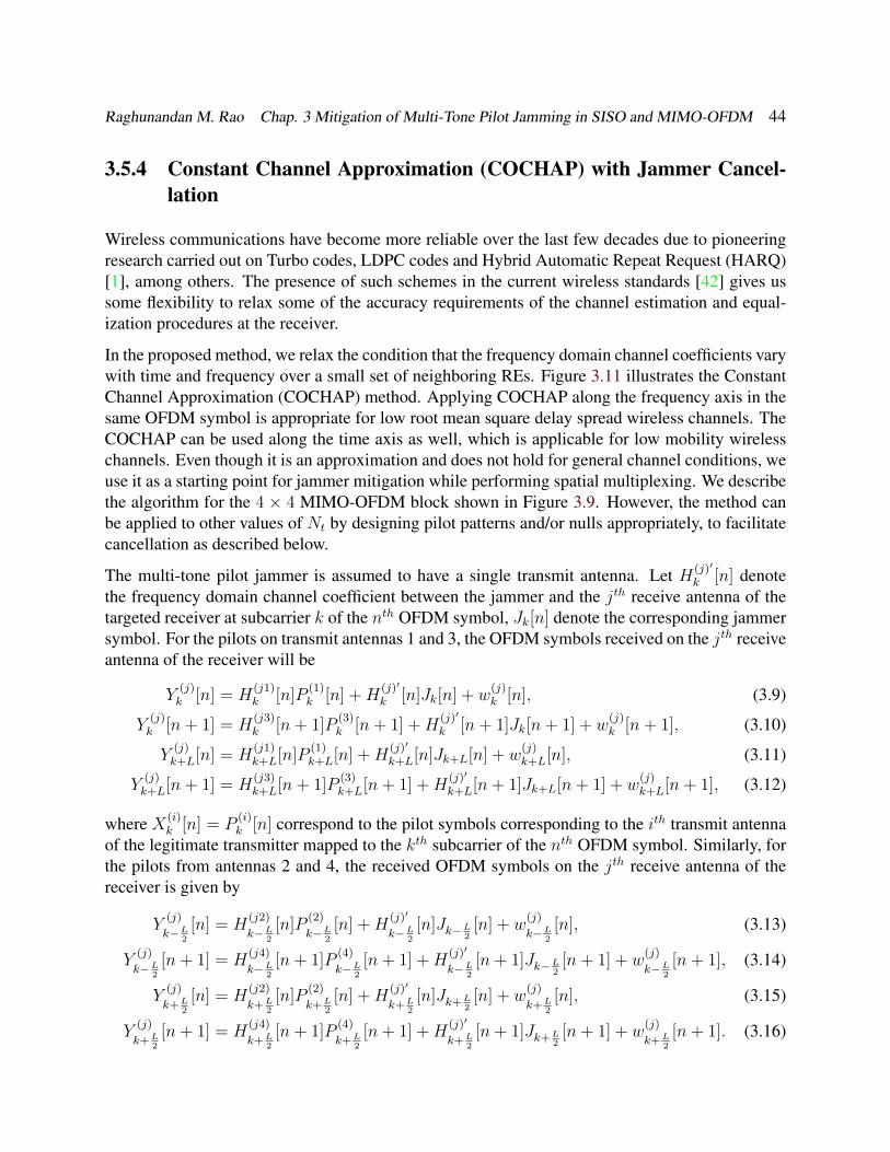
Raghunandan M. Rao Chap. 3 Mitigation of Multi-Tone Pilot Jamming in SISO and MIMO-OFDM 44
3.5.4 Constant Channel Approximation (COCHAP) with Jammer Cancel-lation
Wireless communications have become more reliable over the last few decades due to pioneeringresearch carried out on Turbo codes, LDPC codes and Hybrid Automatic Repeat Request (HARQ)[1], among others. The presence of such schemes in the current wireless standards [42] gives ussome flexibility to relax some of the accuracy requirements of the channel estimation and equal-ization procedures at the receiver.
In the proposed method, we relax the condition that the frequency domain channel coefficients varywith time and frequency over a small set of neighboring REs. Figure 3.11 illustrates the ConstantChannel Approximation (COCHAP) method. Applying COCHAP along the frequency axis in thesame OFDM symbol is appropriate for low root mean square delay spread wireless channels. TheCOCHAP can be used along the time axis as well, which is applicable for low mobility wirelesschannels. Even though it is an approximation and does not hold for general channel conditions, weuse it as a starting point for jammer mitigation while performing spatial multiplexing. We describethe algorithm for the 4 × 4 MIMO-OFDM block shown in Figure 3.9. However, the method canbe applied to other values of Nt by designing pilot patterns and/or nulls appropriately, to facilitatecancellation as described below.
The multi-tone pilot jammer is assumed to have a single transmit antenna. Let H(j)′
k [n] denotethe frequency domain channel coefficient between the jammer and the jth receive antenna of thetargeted receiver at subcarrier k of the nth OFDM symbol, Jk[n] denote the corresponding jammersymbol. For the pilots on transmit antennas 1 and 3, the OFDM symbols received on the jth receiveantenna of the receiver will be
Y(j)k [n] = H
(j1)k [n]P
(1)k [n] +H
(j)′
k [n]Jk[n] + w(j)k [n], (3.9)
Y(j)k [n+ 1] = H
(j3)k [n+ 1]P
(3)k [n+ 1] +H
(j)′
k [n+ 1]Jk[n+ 1] + w(j)k [n+ 1], (3.10)
Y(j)k+L[n] = H
(j1)k+L[n]P
(1)k+L[n] +H
(j)′
k+L[n]Jk+L[n] + w(j)k+L[n], (3.11)
Y(j)k+L[n+ 1] = H
(j3)k+L[n+ 1]P
(3)k+L[n+ 1] +H
(j)′
k+L[n+ 1]Jk+L[n+ 1] + w(j)k+L[n+ 1], (3.12)
where X(i)k [n] = P
(i)k [n] correspond to the pilot symbols corresponding to the ith transmit antenna
of the legitimate transmitter mapped to the kth subcarrier of the nth OFDM symbol. Similarly, forthe pilots from antennas 2 and 4, the received OFDM symbols on the jth receive antenna of thereceiver is given by
Y(j)
k−L2
[n] = H(j2)
k−L2
[n]P(2)
k−L2
[n] +H(j)′
k−L2
[n]Jk−L2[n] + w
(j)
k−L2
[n], (3.13)
Y(j)
k−L2
[n+ 1] = H(j4)
k−L2
[n+ 1]P(4)
k−L2
[n+ 1] +H(j)′
k−L2
[n+ 1]Jk−L2[n+ 1] + w
(j)
k−L2
[n+ 1], (3.14)
Y(j)
k+L2
[n] = H(j2)
k+L2
[n]P(2)
k+L2
[n] +H(j)′
k+L2
[n]Jk+L2[n] + w
(j)
k+L2
[n], (3.15)
Y(j)
k+L2
[n+ 1] = H(j4)
k+L2
[n+ 1]P(4)
k+L2
[n+ 1] +H(j)′
k+L2
[n+ 1]Jk+L2[n+ 1] + w
(j)
k+L2
[n+ 1]. (3.16)
Raghunandan M. Rao Chap. 3 Mitigation of Multi-Tone Pilot Jamming in SISO and MIMO-OFDM 45
Then, the constant channel approximation (COCHAP) is invoked along the frequency axis, for LOFDM subcarriers. Thus for each pilot-bearing OFDM symbol, we model the channel coefficientto be constant for a region of L subcarriers as shown in Figure 3.11. Hence for L
2≤ k ≤ N − L
2
we assume that
H(j1)k [n] ≈ H
(j1)k+L[n],
H(j2)
k−L2
[n] ≈ H(j2)
k+L2
[n],
H(j3)k [n+ 1] ≈ H
(j3)k+L[n+ 1],
H(j4)
k−L2
[n+ 1] ≈ H(j4)
k+L2
[n+ 1]. (3.17)
The jammer channel does not vary appreciably between 2 consecutive OFDM symbols on the samesubcarrier. Also, to minimize power leakage into data subcarriers, the jammer transmits digitallymodulated symbols at a lower data rate than the target OFDM signal. Therefore, we have
H(j)′
k [n] ≈ H(j)′
k [n+ 1]
Jk[n] = Jk[n+ 1]. (3.18)
Using equations (3.10)-(3.18), we get[Y
(j)k [n]− Y (j)
k [n+ 1]
Y(j)k+L[n]− Y (j)
k+L[n+ 1]
]≈
[P
(1)k [n] −P (3)
k [n+ 1]
P(1)k+L[n] −P (3)
k+L[n+ 1]
][H
(j1)k [n]
H(j3)k [n+ 1]
]+ ε
(13)k [n]+[
w(j)k [n]− w(j)
k [n+ 1]
w(j)k+L[n]− w(j)
k+L[n+ 1]
], (3.19)
Y (j)
k−L2
[n]− Y (j)
k−L2
[n+ 1]
Y(j)
k+L2
[n]− Y (j)
k+L2
[n+ 1]
≈P (2)
k−L2
[n] −P (4)
k−L2
[n+ 1]
P(2)
k+L2
[n] −P (4)
k+L2
[n+ 1]
H(j2)
k−L2
[n]
H(j4)
k−L2
[n+ 1]
+ ε(24)k [n]+
w(j)
k−L2
[n]− w(j)
k−L2
[n+ 1]
w(j)
k+L2
[n]− w(j)
k+L2
[n+ 1]
. (3.20)
Parameters ε(13)k [n] and ε(24)
k [n] account for the residual terms due to temporal variations in thechannel between the jammer and the target receiver. The subscripts ε(ij)k [n] denotes that theseresidual terms are a result of signal cancellation between the pilot symbols of antenna ports i andj. They are given as
ε(13)k [n] =
[H
(j)′
k [n]−H(j)′
k [n+ 1] 0
0 H(j)′
k+L[n]−H(j)′
k+L[n+ 1]
][Jk[n]Jk+L[n]
], (3.21)

Raghunandan M. Rao Chap. 3 Mitigation of Multi-Tone Pilot Jamming in SISO and MIMO-OFDM 46
ε(24)k [n] =
H(j)′
k−L2
[n]−H(j)′
k−L2
[n+ 1] 0
0 H(j)′
k+L2
[n]−H(j)′
k+L2
[n+ 1]
[Jk−L2[n]
Jk+L2[n]
]. (3.22)
P(13)k [n] and P
(24)k [n] are defined as
P(13)k [n] ,
[P
(1)k [n] −P (3)
k [n+ 1]
P(1)k+L[n] −P (3)
k+L[n+ 1]
], (3.23)
P(24)k [n] ,
P (2)
k−L2
[n] −P (4)
k−L2
[n+ 1]
P(2)
k+L2
[n] −P (4)
k+L2
[n+ 1]
. (3.24)
We multiply equations (3.19) and (3.20) by (P(13)k [n])−1 and (P
(24)k [n])−1 respectively, to get the
channel estimates at the pilot locations:[H
(j1)k [n]
H(j3)k [n+ 1]
]= (P
(13)k [n])−1
[Y
(j)k [n]− Y (j)
k [n+ 1]
Y(j)k+L[n]− Y (j)
k+L[n+ 1]
]
≈
[H
(j1)k [n]
H(j3)k [n+ 1]
]+ (P
(13)k [n])−1
ε
(13)k [n] +
[w
(j)k [n]− w(j)
k [n+ 1]
w(j)k+L[n]− w(j)
k+L[n+ 1]
],
(3.25)
H(j2)
k−L2
[n]
H(j4)
k−L2
[n+ 1]
= (P(24)k [n])−1
Y (j)
k−L2
[n]− Y (j)
k−L2
[n+ 1]
Y(j)
k+L2
[n]− Y (j)
k+L2
[n+ 1]
≈
H(j2)
k−L2
[n]
H(j4)
k−L2
[n+ 1]
+ (P(24)k [n])−1
ε
(24)k [n] +
w(j)
k−L2
[n]− w(j)
k−L2
[n+ 1]
w(j)
k+L2
[n]− w(j)
k+L2
[n+ 1]
.(3.26)
It is to be noted here that for this method, a pilot sequence of symbols is required for which P(13)k [n]
and P(24)k [n] is invertible for 0 ≤ k ≤ N − 1 and all n. From equations (3.25)-(3.26), we observe
that the accuracy of the channel estimates depends on
1. The variation of the channel coefficient, for the channel between the transmit and receiveantennas, across the L subcarriers, i.e. from subcarrier indices k to k + L, and k − L/2 tok + L/2.
2. The temporal variation of the channel between the jammer and the receiver, represented bythe terms ε(13)
k [n] and ε(24)k [n].
Raghunandan M. Rao Chap. 3 Mitigation of Multi-Tone Pilot Jamming in SISO and MIMO-OFDM 47
3. The jammer power, E[|Jk[n]|2] = σ2J .
4. The SNR on the pilot locations. In fact, the SNR increases by about 3 dB due to directcancellation, even in the case of ε(13)
k [n] = ε(24)k [n] = [0 0]T .
After we obtain the channel estimates on the pilot locations, the channel estimation method de-scribed in section 2.3 can be used to estimate the channel estimates on the data resource elementsof each OFDM block on each spatial layer to obtain Hk[n], for all OFDM symbols, subcarriersand antennas. Hence, it is possible to use multiple spatial layers for increasing throughput, even inthe presence of a multi-tone pilot jammer. However, this comes at the cost of reduced SNR, dueto (a) increased channel estimation MSE as a result of jammer mobility, (b) jammer power and (c)noise enhancement.
In this section we have described the application constant channel approximation along the fre-quency axis, which is applicable in the cases of channels with wide coherence bandwidth. It is alsopossible to apply this approximation along the time axis, which is applicable in the case of lowmobility channels, like in the case pedestrian and low-speed vehicular scenarios.
3.5.5 Numerical Results
In this section we demonstrate the performance of the proposed COCHAP with jammer cancella-tion method for mitigating multi-tone pilot jamming. We use a 4× 4 MIMO-OFDM system, witheach spatial layer having OFDM block parameters as shown in Table 2.2. We have consideredQPSK modulated symbols at each data resource element. For full rank spatial multiplexing, wehave assumed the transmit and receive angle spreads to be 2π radians. We have assumed the trans-mitter and receiver antenna spacing to be dt = [0 3λ 6λ 9λ] and dr = [0 λ 2λ 3λ] respectively,where λ = c/fc is the wavelength of the center subcarrier. The pilot pattern used for each spatiallayer is shown in Figure 3.9.
We consider the following scenarios:
1. Synchronous multi-tone pilot jamming with no mitigation. The jammer does not transmit onresource elements other than the ones occupied by pilots.
2. No Jamming.
3. Mitigation of multi-tone pilot jamming using COCHAP with jammer cancellation along thefrequency axis.
We evaluate the effectiveness of our mitigation scheme based on two metrics: BER and ErgodicSum Capacity. Ergodic Sum Capacity Cs is indicative of the throughput achievable in the case of

Raghunandan M. Rao Chap. 3 Mitigation of Multi-Tone Pilot Jamming in SISO and MIMO-OFDM 48
a full spatial-multiplexing based MIMO-OFDM system, given by [47]
Cs = Bsc
Nt∑i=1
En[ ∑k/∈Pi[n]
log2(1 + γk,i[n])], (3.27)
where Bsc is the bandwidth per OFDM subcarrier, γk,i[n] is the SINR of the resource element ofthe ith spatial layer, kth subcarrier and the nth OFDM symbol. En[.] denotes the expectation w.r.t.the time variable n. Pi[n] denotes the set of pilot locations mapped to the ith spatial layer at thenth OFDM symbol. Note that pilot REs do not contribute to the capacity as they do not carry data.
Figures 3.12, 3.13 and 3.14 show the Ergodic Sum Capacity for all considered scenarios, for(τrms, fd) = (100 ns, 50 Hz), (τrms, fd) = (200 ns, 100 Hz), and (τrms, fd) = (400 ns, 200 Hz)respectively. We see that multi-tone pilot jamming reduces the channel capacity by a factor of4− 5, at Eb/N0 = 30 dB for all considered channel environments. With conventional beamform-ing, the capacity would scale by a maximum factor of log2(Nr) = log2(4) = 2 at a very high SINR[44]. On the other hand, when COCHAP with Jammer Cancellation is used along the frequencyaxis, it is able to achieve ∼ 50− 90% of the Ergodic Sum capacity w.r.t. that in the case of a 4× 4MIMO-OFDM system with full rank spatial multiplexing in absence of a jammer.
Figures 3.15, 3.16 and 3.17 show the BER comparison for all considered scenarios, for (τrms, fd) =(100 ns, 50 Hz), (τrms, fd) = (200 ns, 100 Hz), and (τrms, fd) = (400 ns, 200 Hz) respectively.Similar to what we observed in the SISO-OFDM case for QPSK-modulated data symbols, weobserve a BER improvement by 1− 2 orders magnitude when COCHAP with JC is used.
An immediate consequence of direct cancellation of signals on adjacent pilot REs is the 3 dBdrop in the SINR, as seen in equation (3.19)-(3.20). This can be observed in Figures 3.12 and 3.15,where the COCHAP with JC curves are shifted to the right by≈ 3 dB w.r.t. the performance curvesof the no jamming case. This is because of the low channel variation along the time and frequencyaxes, which yields very small values for ε(13)
k [n] and ε(24)k [n] terms in equations (3.19)-(3.20). As
one would expect, the effectiveness of our proposed mitigation strategy is sensitive to the channelcharacteristics between the transmitter and the receiver, and between the jammer and the receiver.The performance of this mitigation strategy is acceptable for τrms = 0 − 200 ns and fd = 0 −100 Hz, which translate to low root mean square delay spread and low mobility scenarios. Thecapacity scaling of spatial multiplexing is sensitive to angular spreads at the receive antenna. Lowr.m.s. delay spreads of ∼ 50 ns has been shown to be possible in outdoor to indoor channelenvironments [14]. Thus, in outdoor-to-indoor and some outdoor-to-outdoor scenarios, COCHAPwith JC would be expected to enable full rank spatial-multiplexing operation with as low as 9% lossin throughput, in the presence of a multi-tone pilot jammer. Another approach to deal with channelvariations in high r.m.s. delay spread and mobile channels, is to densify the pilot pattern. In thiscase, constant channel approximation becomes more accurate and can yield better performanceeven in such scenarios, but at the cost of a marginal reduction in throughput due to the additionalpilot overhead.

Raghunandan M. Rao Chap. 3 Mitigation of Multi-Tone Pilot Jamming in SISO and MIMO-OFDM 49
5 10 15 20 25 300
5
10
15
20
25
30
Average Eb/N
0 (dB)
Erg
od
ic S
um
Ca
pa
city (
bp
s/H
z)
COCHAP with JC, JSR = −5dBCOCHAP with JC, JSR = 0dBCOCHAP with JC, JSR = 5dBNo Mitigation, JSR = −5dBNo Mitigation, JSR = 0dBNo Mitigation, JSR = 5dBNo Jamming
Figure 3.12: Comparison of Ergodic sum capacity for all scenarios, for τrms = 100 ns, fd = 50 Hz.
5 10 15 20 25 300
5
10
15
20
25
30
Average Eb/N
0 (dB)
Erg
od
ic S
um
Ca
pa
city (
bp
s/H
z)
COCHAP with JC, JSR = −5dBCOCHAP with JC, JSR = 0dBCOCHAP with JC, JSR = 5dBNo Mitigation, JSR = −5dBNo Mitigation, JSR = 0dBNo Mitigation, JSR = 5dBNo Jamming
Figure 3.13: Comparison of Ergodic sum capacity for all scenarios, for τrms = 200 ns, fd =100 Hz.

Raghunandan M. Rao Chap. 3 Mitigation of Multi-Tone Pilot Jamming in SISO and MIMO-OFDM 50
5 10 15 20 25 300
5
10
15
20
25
30
Average Eb/N
0 (dB)
Erg
od
ic S
um
Ca
pa
city (
bp
s/H
z)
No JammingNo Mitigation, JSR = −5dBNo Mitigation, JSR = 0dBNo Mitigation, JSR = 5dBCOCHAP with JC, JSR = −5dBCOCHAP with JC, JSR = 0dBCOCHAP with JC, JSR = 5dB
Figure 3.14: Comparison of Ergodic sum capacity for all scenarios, for τrms = 400 ns, fd =200 Hz.
Average Eb/N
0 (dB)
5 10 15 20 25 30
BE
R
10-4
10-3
10-2
10-1
100
No Jamming
No Mitigation, JSR = -5dB
No Mitigation, JSR = 0dB
No Mitigation, JSR = 5dB
COCHAP with JC, JSR = -5dB
COCHAP with JC, JSR = 0dB
COCHAP with JC, JSR = 5dB
Figure 3.15: Comparison of Bit Error Rate for all scenarios, for τrms = 100 ns, fd = 50 Hz.

Raghunandan M. Rao Chap. 3 Mitigation of Multi-Tone Pilot Jamming in SISO and MIMO-OFDM 51
Average Eb/N
0 (dB)
5 10 15 20 25 30
BE
R
10-3
10-2
10-1
100
No Jamming
No Mitigation, JSR = -5dB
No Mitigation, JSR = 0dB
No Mitigation, JSR = 5dB
COCHAP with JC, JSR = -5dB
COCHAP with JC, JSR = 0dB
COCHAP with JC, JSR = 5dB
Figure 3.16: Comparison of Bit Error Rate for all scenarios, for τrms = 200 ns, fd = 100 Hz.
Average Eb/N
0 (dB)
5 10 15 20 25 30
BE
R
10-3
10-2
10-1
No Mitigation, JSR = -5dB
No Mitigation, JSR = 0dB
No Mitigation, JSR = 5dB
COCHAP with JC, JSR = -5dB
COCHAP with JC, JSR = 0dB
COCHAP with JC, JSR = 5dB
No Jamming
Figure 3.17: Comparison of Bit Error Rate for all scenarios, for τrms = 400 ns, fd = 200 Hz.
Raghunandan M. Rao Chap. 3 Mitigation of Multi-Tone Pilot Jamming in SISO and MIMO-OFDM 52
3.6 Conclusions
In this chapter, we proposed strategies to mitigate a power-constrained multi-tone pilot jammer inSISO- and MIMO-OFDM systems. The main goal of the mitigation strategies is to restore channelestimation performance in the presence of the jammer. We saw that for the case of SISO-OFDMsystems:
1. Synchronous pilot jamming is a very efficient attack, but jammer evasion can restore theBER performance because the data REs being interfered constitute a small fraction of thetotal number of data REs.
2. Asynchronous pilot jamming is a very simple attack, but the data subcarriers on pilot fre-quencies are unnecessarily affected. In this case, schemes like Adaptive Modulation andCoding, Hybrid ARQ (HARQ), lower coding rates etc. are necessary to restore the BERperformance. However, RE Blanking with JC helps in restoring the channel estimation per-formance, without which the aforementioned auxiliary schemes would be ineffective if im-plemented all by themselves.
We also investigated whether full rank spatial multiplexing operation is possible in a MIMO-OFDM system in the presence of a multi-tone pilot jammer. We devised and demonstrated amitigation strategy called Constant Channel Approximation (COCHAP) with Jammer Cancella-tion. It is capable of restoring ∼ 50 − 90% of the Ergodic Sum Capacity w.r.t. that of a fullrank spatial multiplexing system, for 4 × 4 MIMO-OFDM. For very high r.m.s. delay spreads(τrms > 500 ns) and low-mobility scenarios (fd = 0− 100 Hz at fc = 2 GHz), COCHAP with JCcan be applied temporally to restore full rank spatial multiplexing operation.
In addition to these methods, it is evident that adaptation of pilot spacing and/or locations in theOFDM block, can intrinsically be a deterrent against pilot jamming. This aspect, in addition withthe traditional benefits of throughput maximization is explored in Chapter 5.
Chapter 4
Jamming of LTE’s Cell-Specific ReferenceSignal (CRS)
4.1 Background
The Long Term Evolution (LTE) was standardized by the Third Generation Partnership Project(3GPP), to address the rapid surge in cellular data traffic over the last decade. LTE providestremendous performance enhancements over its predecessors in terms of data rate, latency, cover-age and mobility management. Hence, LTE/LTE-A has received a lot of support from the R&Dcommunity and it promises to become the primary standard for a broad range of wireless networks,including public safety and military [48]. But, since it is openly documented and widely deployed,it becomes an easy target to intentional and unintentional interference. Hence, it is important toidentify vulnerabilities of LTE and make future releases more resilient to targeted interference.
There has been prior work related to RF Jamming of LTE signals. Kakar et al. [15] investigatethe performance of the Physical Control Format Indicator Channel (PCFICH) under harsh wirelessconditions and propose strategies to mitigate interference on the PCFICH. Lichtman et al. [16]consider the problem of targeted interference on the Physical Uplink Control Channel (PUCCH)and propose detection and mitigation strategies to counter protocol-aware jammers. Labib et al.[17] introduce and demonstrate LTE control channel spoofing, which refers to spoofing by a fakeeNodeB by transmission of a partial LTE downlink frame. Denial of Service (DoS) was found tobe the result of transmission of the partial LTE downlink frames containing only the fake controlchannels, at a relatively higher power level w.r.t. the legitimate eNodeB. The authors also pro-pose mitigation strategies that required simple modification to the cell selection process of LTE.In [18], a comprehensive threat assessment of LTE/LTE-A is provided, highlighting the vulnera-bilities of various LTE physical channels and signals. A survey of mitigation techniques againstvarious jamming/spoofing attacks is also provided. Jover et al. [19] focus on the jamming of LTEnetworks, and overviews power-efficient jamming attacks. They propose a series of security re-
53
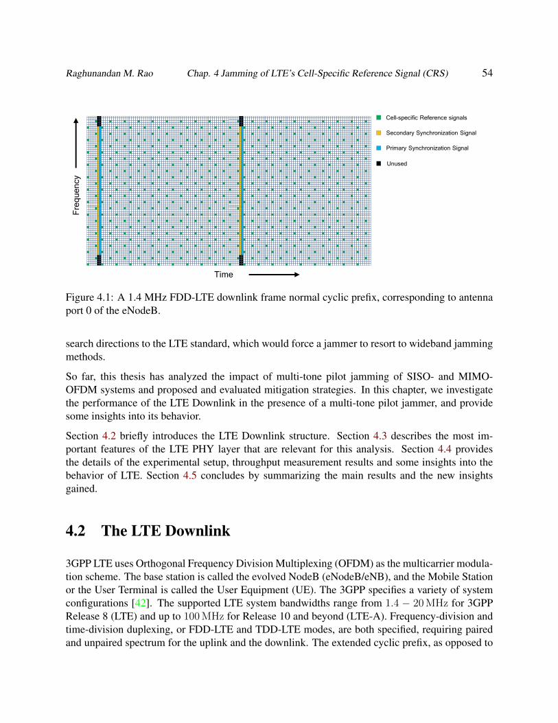
Raghunandan M. Rao Chap. 4 Jamming of LTE’s Cell-Specific Reference Signal (CRS) 54
Cell-specific Reference signals
Secondary Synchronization Signal
Primary Synchronization Signal
Unused
Fre
qu
en
cy
Time
Figure 4.1: A 1.4 MHz FDD-LTE downlink frame normal cyclic prefix, corresponding to antennaport 0 of the eNodeB.
search directions to the LTE standard, which would force a jammer to resort to wideband jammingmethods.
So far, this thesis has analyzed the impact of multi-tone pilot jamming of SISO- and MIMO-OFDM systems and proposed and evaluated mitigation strategies. In this chapter, we investigatethe performance of the LTE Downlink in the presence of a multi-tone pilot jammer, and providesome insights into its behavior.
Section 4.2 briefly introduces the LTE Downlink structure. Section 4.3 describes the most im-portant features of the LTE PHY layer that are relevant for this analysis. Section 4.4 providesthe details of the experimental setup, throughput measurement results and some insights into thebehavior of LTE. Section 4.5 concludes by summarizing the main results and the new insightsgained.
4.2 The LTE Downlink
3GPP LTE uses Orthogonal Frequency Division Multiplexing (OFDM) as the multicarrier modula-tion scheme. The base station is called the evolved NodeB (eNodeB/eNB), and the Mobile Stationor the User Terminal is called the User Equipment (UE). The 3GPP specifies a variety of systemconfigurations [42]. The supported LTE system bandwidths range from 1.4 − 20 MHz for 3GPPRelease 8 (LTE) and up to 100 MHz for Release 10 and beyond (LTE-A). Frequency-division andtime-division duplexing, or FDD-LTE and TDD-LTE modes, are both specified, requiring pairedand unpaired spectrum for the uplink and the downlink. The extended cyclic prefix, as opposed to

Raghunandan M. Rao Chap. 4 Jamming of LTE’s Cell-Specific Reference Signal (CRS) 55
the normal cyclic prefix configuration, can account for longer root mean square delay spreads.
Figure 4.1 shows a simplified 1.4 MHz FDD-LTE downlink frame, highlighting the most importantLTE physical control signals. Signals exist only at the physical layer, whereas physical channelsare mapped to transport and logical channels. The frame structure in TDD-LTE is similar to thatof FDD-LTE, except for the guard intervals between uplink and downlink frames. Of the manyimportant downlink control channels of LTE, the control signals of interest in this work is thecell-specific reference signal (CRS). These are the pilot signals broadcasted in the downlink, andare used for channel estimation and equalization are carried out at the User Equipment (UE). In asingle cell, up to 4 different groups of CRSs can be transmitted. Each of these patterns correspondsto a specific antenna port. This is to support up to 4×4 MIMO in the Downlink. The configurationin Figure 4.1 corresponds to the frame that would be transmitted out of antenna port 0 in a multi-antenna system [1]. This particular diamond shaped arrangement with homogeneous subcarrierspacing achieves the minimum mean square error (MMSE) of the channel estimate [25].
The CRS subcarriers are determined by the cell identity Nc,ID, which can take any integer valuefrom 0 to 503. The pattern shown in Figure 4.1 corresponds toNc,ID = 0. A cell-specific frequencyshift of ∆f = [Nc,ID (mod 6)] × ∆fsc is applied to the pattern in a cell with cell ID of Nc,ID,where ∆fsc = 15 kHz. In addition to aiding in channel estimation, CRS is also used to
1. Estimate channel quality parameters like Reference Signal Received Power (RSRP) and Ref-erence Signal Received Quality (RSRQ). These are important parameters for cell selectionand reselection (handover) [1].
2. Derive the channel state information (CSI) for its antenna port aiding in link adaptation,precoding selection, etc. [1].
In order to allow accurate estimation of the above parameters in low SINR environments, relativeCRS power boosting (w.r.t. data symbols) of upto 6 dB is allowed in LTE [1]. Because of thefixed CRS positions in the LTE grid, it would be easy for a jammer to transmit interfering signalson (a) these subcarriers (asynchronous jammer), (b) the exact CRS locations (synchronous, mostlikely a reactive jammer), or (c) a combination of both with intermittent transmission. Moreover,in the case of frequency reuse factor of 1, the jammer can go to the cell-edge region of 3 adjacentcells, assume any value of Nc,ID and target the appropriate CRS subcarriers in order to interferewith that cell. In this case, 1 out of the 3 cells will face network congestion or outage, based onthe jammer power and the channel environment. Network congestion can occur in the case when(a) the jammer power is not strong enough to cause DoS or (b) DoS in one cell causes networkcongestion in adjacent cells due to load balancing. Hence, the PHY layer issues of the network inone cell can potentially translate into coverage and network congestion in the surrounding cells.
Raghunandan M. Rao Chap. 4 Jamming of LTE’s Cell-Specific Reference Signal (CRS) 56
4.3 Channel Quality and Adaptive Modulation and Coding
In cellular systems, the measurement of channel quality is necessary in order to optimize the systemperformance in terms of coverage and throughput for a given transmit power. In LTE, channelquality is estimated using a parameter called the Channel Quality Indicator (CQI), which is fedback to the eNB/UE by the UE/eNB for the downlink/uplink adaptation respectively. Using thisfed back CQI, the modulation and coding scheme (MCS) is updated. In LTE, MCS dictates themodulation order and coding scheme used by the UE/eNB in the uplink/downlink [41]. There are32 possible values for the MCS in the uplink and the downlink [2]. Higher order modulation ismore susceptible to interference while lower order modulation schemes are more robust. Similarly,higher code rates are more vulnerable to interference while lower code rates are more resilientagainst it. There is a tradeoff between throughput and resilience to noise and interference. Ingeneral, higher modulation orders and coding rates result in higher throughput, and vice versa.
If the reported CQI value is high, a higher order modulation and coding rate is chosen and viceversa. This is termed as Link Adaptation, where the reported CQI value is used to choose theMCS. Since the MCS is adapted based on varying channel quality, it is referred to as AdaptiveModulation and Coding in LTE. The CQI in 3GPP LTE is defined as follows [2]:
“A single PDSCH transport block with a combination of modulation scheme and transport blocksize corresponding to the CQI index, and occupying a group of downlink physical resource blockstermed the CSI reference resource, could be received with a transport block error probability notexceeding 0.1.”
In other words, CQI maps to a MCS so that the transport blocks can be decoded with a Block Errorrate (BLER) of 10% or less. In LTE, the CQI values vary from 0 to 15, and the MCS values varyfrom 0 to 31. The mapping from CQI to the spectral efficiency for 3GPP LTE Release 8 is shownin Table 4.1 [1]. 3GPP Release 12 supports 256QAM as well, resulting in much higher spectralefficiency of up to 7.4063 bps/Hz [2]. There are different types of CQI, with different definitionsand reporting intervals. The interested reader is encouraged to refer to the 3GPP standardizationdocuments [2] for more information. For the purpose of our understanding and analysis of pilotjamming in LTE, it is sufficient to understand that the fed back CQI dictates the modulation andcoding scheme employed by the transmitter. The maximum theoretical throughput achievable bythe downlink of 10 MHz FDD LTE in a SISO configuration, is shown in Table 4.2 for each MCSvalue. The interested user is referred to [2] to compute the maximum theoretical throughput fordifferent configurations and 3GPP-LTE releases.
4.4 Impact of CRS Jamming on the Performance of LTE
Since CRS is the downlink pilots broadcasted to all the UEs, we will henceforth refer to multi-tone pilot jamming as CRS jamming in the context of LTE. The aim of this jammer could be to(a) throttle the throughput of the cell in order to degrade network performance or (b) cause DoS
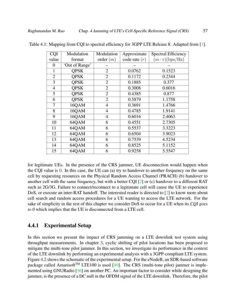
Raghunandan M. Rao Chap. 4 Jamming of LTE’s Cell-Specific Reference Signal (CRS) 57
Table 4.1: Mapping from CQI to spectral efficiency for 3GPP LTE Release 8. Adapted from [1].
CQI Modulation Modulation Approximate Spectral Efficiencyvalue format order (m) code rate (r) (m · r)(bps/Hz)
0 ‘Out of Range’ – – –1 QPSK 2 0.0762 0.15232 QPSK 2 0.1172 0.23443 QPSK 2 0.1885 0.3774 QPSK 2 0.3008 0.60165 QPSK 2 0.4385 0.8776 QPSK 2 0.5879 1.17587 16QAM 4 0.3691 1.47668 16QAM 4 0.4785 1.91419 16QAM 4 0.6016 2.4063
10 64QAM 6 0.4551 2.730511 64QAM 6 0.5537 3.322312 64QAM 6 0.6504 3.902313 64QAM 6 0.7539 4.523414 64QAM 6 0.8525 5.115215 64QAM 6 0.9258 5.5547
for legitimate UEs. In the presence of the CRS jammer, UE disconnection would happen whenthe CQI value is 0. In this case, the UE can (a) try to handover to another frequency on the samecell by requesting resources on the Physical Random Access Channel (PRACH) (b) handover toanother cell with the same frequency, but with a better CQI [2] or (c) handover to a different RATsuch as 2G/3G. Failure to connect/reconnect to a legitimate cell will cause the UE to experienceDoS, or execute an inter-RAT handoff. The interested reader is directed to [2] to know more aboutcell search and random access procedures for a UE wanting to access the LTE network. For thesake of simplicity in the rest of this chapter we consider DoS to occur for a UE when its CQI goesto 0 which implies that the UE is disconnected from a LTE cell.
4.4.1 Experimental Setup
In this section we present the impact of CRS jamming on a LTE downlink test system usingthroughput measurements. In chapter 3, cyclic shifting of pilot locations has been proposed tomitigate the multi-tone pilot jammer. In this section, we investigate its performance in the contextof the LTE downlink by performing an experimental analysis with a 3GPP-compliant LTE system.Figure 4.2 shows the schematic of the experimental setup. For the eNodeB, an SDR-based softwarepackage called AmarisoftTM LTE100 is used [49]. The CRS (multi-tone pilot) jammer is imple-mented using GNURadio [50] on another PC. An important factor to consider while designing thejammer, is the presence of a DC null in the OFDM signal of the LTE downlink. Therefore, the pilot
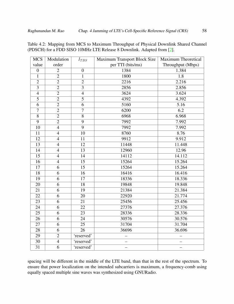
Raghunandan M. Rao Chap. 4 Jamming of LTE’s Cell-Specific Reference Signal (CRS) 58
Table 4.2: Mapping from MCS to Maximum Throughput of Physical Downlink Shared Channel(PDSCH) for a FDD SISO 10MHz LTE Release 8 Downlink. Adapted from [2].
MCS Modulation ITBS Maximum Transport Block Size Maximum Theoreticalvalue order per TTI (bits/ms) Throughput (Mbps)
0 2 0 1384 1.3841 2 1 1800 1.82 2 2 2216 2.2163 2 3 2856 2.8564 2 4 3624 3.6245 2 5 4392 4.3926 2 6 5160 5.167 2 7 6200 6.28 2 8 6968 6.9689 2 9 7992 7.992
10 4 9 7992 7.99211 4 10 8760 8.7612 4 11 9912 9.91213 4 12 11448 11.44814 4 13 12960 12.9615 4 14 14112 14.11216 4 15 15264 15.26417 6 15 15264 15.26418 6 16 16416 16.41619 6 17 18336 18.33620 6 18 19848 19.84821 6 19 21384 21.38422 6 20 22920 21.77423 6 21 25456 25.45624 6 22 27376 27.37625 6 23 28336 28.33626 6 24 30576 30.57627 6 25 31704 31.70428 6 26 36696 36.69629 2 ‘reserved’ – –30 4 ‘reserved’ – –31 6 ‘reserved’ – –
spacing will be different in the middle of the LTE band, than that in the rest of the spectrum. Toensure that power localization on the intended subcarriers is maximum, a frequency-comb usingequally spaced multiple sine waves was synthesized using GNURadio.
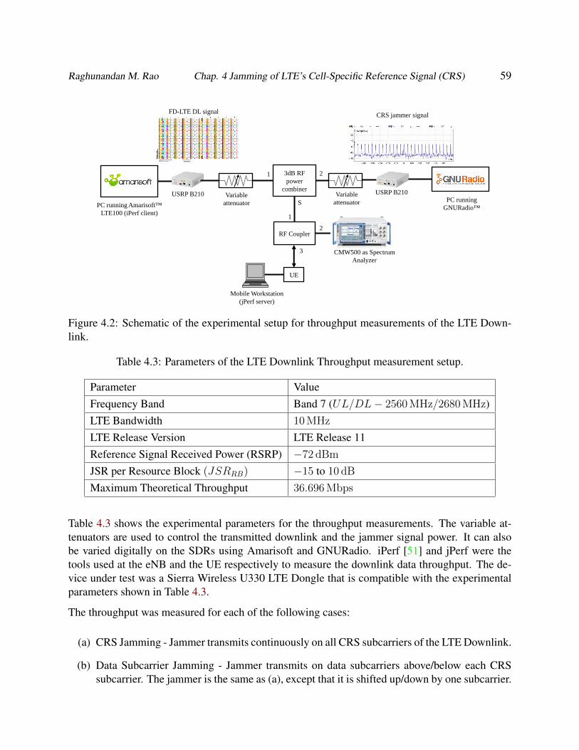
Raghunandan M. Rao Chap. 4 Jamming of LTE’s Cell-Specific Reference Signal (CRS) 59
FD-LTE DL signal
PC running Amarisoft™
LTE100 (iPerf client)
3dB RF
power
combiner
PC running
GNURadio™
RF Coupler
UE
Mobile Workstation
(jPerf server)
CMW500 as Spectrum
Analyzer
CRS jammer signal
USRP B210
1 2
S
1
2
3
USRP B210 Variable
attenuator
Variable
attenuator
Figure 4.2: Schematic of the experimental setup for throughput measurements of the LTE Down-link.
Table 4.3: Parameters of the LTE Downlink Throughput measurement setup.
Parameter ValueFrequency Band Band 7 (UL/DL− 2560 MHz/2680 MHz)LTE Bandwidth 10 MHz
LTE Release Version LTE Release 11Reference Signal Received Power (RSRP) −72 dBm
JSR per Resource Block (JSRRB) −15 to 10 dB
Maximum Theoretical Throughput 36.696 Mbps
Table 4.3 shows the experimental parameters for the throughput measurements. The variable at-tenuators are used to control the transmitted downlink and the jammer signal power. It can alsobe varied digitally on the SDRs using Amarisoft and GNURadio. iPerf [51] and jPerf were thetools used at the eNB and the UE respectively to measure the downlink data throughput. The de-vice under test was a Sierra Wireless U330 LTE Dongle that is compatible with the experimentalparameters shown in Table 4.3.
The throughput was measured for each of the following cases:
(a) CRS Jamming - Jammer transmits continuously on all CRS subcarriers of the LTE Downlink.
(b) Data Subcarrier Jamming - Jammer transmits on data subcarriers above/below each CRSsubcarrier. The jammer is the same as (a), except that it is shifted up/down by one subcarrier.

Raghunandan M. Rao Chap. 4 Jamming of LTE’s Cell-Specific Reference Signal (CRS) 60
Jammed CRS
Interference-free
data resource
elements
Jammed data
resource elements
Interference-free
CRS
(a) CRS Jamming (a) Data subcarrier
Jamming(c) Barrage Jammingtime
freq
uen
cy
Figure 4.3: Schematic of the jamming strategies investigated for throughput performance of theLTE downlink. The number of REs affected are the same in CRS and data subcarrier jamming.
(c) Barrage Jamming - Jammer transmits on all LTE Downlink subcarriers.
Figure 4.3 shows the schematic of these jamming strategies.
4.4.2 Throughput Measurement Results
The transmit power of the eNB was kept constant and downlink data transfer was carried out usingan iPerf client (at the eNB) and jPerf server (at the UE). iPErf and jPerf was configured to makesure that the data buffers were always full. The jammer power is held constant during a downlinkdata transfer duration of 100 s and the average throughput over this duration was measured for afixed value of JSR per resource block (JSRRB).
Definition 4.1. Jammer to Signal ratio per Resource Block (JSRRB) is defined as
JSRRB =P JRB
PLTE,RB(4.1)
where PLTE,RB is the average power of the LTE DL signal per Resource block, and P JRB is the
jammer power per Resource block.
In cases (a) and (b), only one out of every three subcarriers of the LTE DL frame are targeted whilein case (c) all subcarriers are targeted. JSRRB was varied from -15 to +10dB while repeatingthe above procedure for each value of JSRRB, which constitutes a single trial. For each of the

Raghunandan M. Rao Chap. 4 Jamming of LTE’s Cell-Specific Reference Signal (CRS) 61
three considered jamming scenarios, four trials were performed and the statistics of the measuredthroughput values were computed to check the consistency of the measurements for each trial. Thevariance of measured throughput, averaged across all JSRRB values over four trials were σCRS =0.36 Mbps, σdata = 0.541 Mbps, σbarr = 0.123 Mbps. The subscripts CRS, data, and barr referto the cases of CRS, data and barrage jamming respectively. Hence, the throughput variationremains consistent within reasonable values for the considered range of JSRRB, allowing us togain insights about the behavior of the LTE DL under these three jamming scenarios. The readeris referred to Appendix A for more details regarding the throughput measurements.
In the rest of this section henceforth, all the figures are equipped with error bars. The height fromthe center to the top of error bar represents the variance of measured throughput for the corre-sponding JSRRB value. Figure 4.4 shows the comparison between the throughput performanceof all the above considered jamming scenarios. As expected, we see that barrage jamming needs∼ 5 dB more jammer power than the other 2 cases. However, it is interesting and somewhatcounter-intuitive to see the following: a) jamming of 1 out of 3 data subcarriers (jamming scenario(b)) performs comparable to CRS jamming, and b) DoS, which essentially is the disconnection ofthe UE happens at around the same value of JSRRB for both CRS and data subcarrier jamming.This behavior is the opposite of what was predicted in the theoretical results of Chapter 3. Sincethe CRS is not corrupted with interference the throughput performance would be expected to bebetter than that in CRS jamming. But the outcome of our experiments is opposite to our initialhypothesis.
−15 −10 −5 0 5 100
2
4
6
8
10
12
14
16
18
20
Jammer to Signal Ratio per Resource Block (dB)
Th
rou
gh
pu
t (M
bp
s)
Rmeas - CRS jamming
Rmeas - data subcarrier jamming
Rmeas - barrage jamming
Figure 4.4: Measured throughput versus JSR per Resource Block for all considered jammingschemes.
Raghunandan M. Rao Chap. 4 Jamming of LTE’s Cell-Specific Reference Signal (CRS) 62
To investigate this anomalous behavior, the CQI and MCS values were monitored throughout theduration of the throughput measurements. Using Tables 4.1 and 4.2, the maximum achievablethroughput for the measured MCS was computed. Figure 4.5 shows the theoretical value of themaximum achievable throughput for the LTE downlink, computed using the monitored CQI andMCS values for each trial. At this point, we define a metric called the achievable throughputefficiency which is a measure of the throughput achieved w.r.t. the maximum throughput achievablein ideal conditions.
Definition 4.2. Achievable Throughput efficiency (ηach,th) for a measured duration Tmeas is givenby
ηach,th =Rmeas
Rmax,MCS
(4.2)
where Rmeas is the average measured throughput for the duration of Tmeas seconds, and Rmax,MCS
the maximum possible throughput achievable for the median MCS value chosen by the eNB duringthe same duration. Rmax,MCS can be computed for the corresponding measured MCS value usingTable 4.2.
Figure 4.6 shows the throughput efficiency for all jamming scenarios, which shows the severethroughput degradation in data subcarrier jamming (1 in 3 subcarriers). For CRS and Barragejamming, the throughput efficiency ranges from 80 − 90% for low JSRRB values. However, theefficiency for jamming of 1 in 3 data subcarriers is 10 − 50% in the same range of JSRRB. Wedefine throughput efficiency as the ratio of the measured throughput to the maximum achievablethroughput for the average MCS value chosen during the measurement duration.
The reason for the low throughput in case of data subcarrier jamming is revealed in Figures 4.5and 4.6. It is due to the inability of the UE to accurately estimate the CQI in this jamming scheme.Typically the CQI estimation algorithm is left to the UE manufacturer, but the most commonunderlying approach is estimation of the noise and interference variance or the SINR [1]. Differentmethods have been suggested in the literature to estimate CQI, among which pilot-based noisevariance estimation is popular [52, 53]. Pilot signals are known to the UE which simplifies thenoise and interference variance estimation.
Hence in the case of CRS jamming, the interference on the pilots will result in accurate trackingof the CQI because the interference is aligned with the CRS subcarriers. However, in the caseof localized multi-channel data jamming, the absence of interference on the CRS will lead tohigh CQI values which in return map to a high MCS value. It is well known that higher ordermodulation schemes (e.g. 16QAM, 64QAM) are not resilient to low SINRs, which result in ahigh percentage of retransmissions of > 50%. A direct consequence of higher retransmissionsand BLER, is degraded throughput performance. We term this phenomenon as ‘CQI Spoofing’,where the UE is tricked by the jammer into incorrectly estimating CQI values to be high, even inthe presence of strong targeted interference. The impact of spoofing is severe when the jammertransmits almost the same power per targeted RE (note that only 1 out of 3 subcarriers are targeted)as the LTE signal, which is represented by the kinks near JSRRB = −5 dB in Figure 4.4. It is
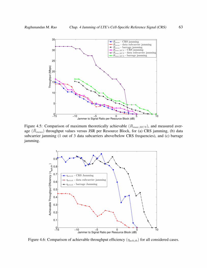
Raghunandan M. Rao Chap. 4 Jamming of LTE’s Cell-Specific Reference Signal (CRS) 63
−15 −10 −5 0 5 100
5
10
15
20
25
30
35
Jammer to Signal Ratio per Resource Block (dB)
Th
rou
gh
pu
t (M
bp
s)
Rmeas - CRS jammingRmeas - data subcarrier jammingRmeas - barrage jammingRmax,MCS - CRS jammingRmax,MCS - data subcarrier jammingRmax,MCS - barrage jamming
Figure 4.5: Comparison of maximum theoretically achievable (Rmax,MCS), and measured aver-age (Rmeas) throughput values versus JSR per Resource Block, for (a) CRS jamming, (b) datasubcarrier jamming (1 out of 3 data subcarriers above/below CRS frequencies), and (c) barragejamming.
−15 −10 −5 0 5 100
0.1
0.2
0.3
0.4
0.5
0.6
0.7
0.8
0.9
1
Jammer to Signal Ratio per Resource Block (dB)
Achie
vable
Thro
ughput E
ffic
iency (
ηach,th )
ηach,th - CRS Jamming
ηach,th - data subcarrier jamming
ηach,th - barrage Jamming
Figure 4.6: Comparison of achievable throughput efficiency (ηach,th) for all considered cases.
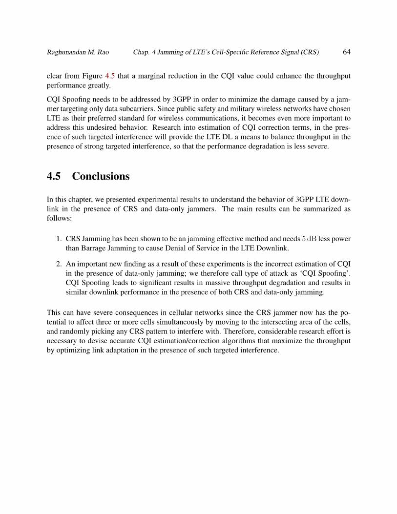
Raghunandan M. Rao Chap. 4 Jamming of LTE’s Cell-Specific Reference Signal (CRS) 64
clear from Figure 4.5 that a marginal reduction in the CQI value could enhance the throughputperformance greatly.
CQI Spoofing needs to be addressed by 3GPP in order to minimize the damage caused by a jam-mer targeting only data subcarriers. Since public safety and military wireless networks have chosenLTE as their preferred standard for wireless communications, it becomes even more important toaddress this undesired behavior. Research into estimation of CQI correction terms, in the pres-ence of such targeted interference will provide the LTE DL a means to balance throughput in thepresence of strong targeted interference, so that the performance degradation is less severe.
4.5 Conclusions
In this chapter, we presented experimental results to understand the behavior of 3GPP LTE down-link in the presence of CRS and data-only jammers. The main results can be summarized asfollows:
1. CRS Jamming has been shown to be an jamming effective method and needs 5 dB less powerthan Barrage Jamming to cause Denial of Service in the LTE Downlink.
2. An important new finding as a result of these experiments is the incorrect estimation of CQIin the presence of data-only jamming; we therefore call type of attack as ‘CQI Spoofing’.CQI Spoofing leads to significant results in massive throughput degradation and results insimilar downlink performance in the presence of both CRS and data-only jamming.
This can have severe consequences in cellular networks since the CRS jammer now has the po-tential to affect three or more cells simultaneously by moving to the intersecting area of the cells,and randomly picking any CRS pattern to interfere with. Therefore, considerable research effort isnecessary to devise accurate CQI estimation/correction algorithms that maximize the throughputby optimizing link adaptation in the presence of such targeted interference.
Chapter 5
Adaptation of Pilot Patterns for OFDMSystems
5.1 Introduction
In current wireless standards based on OFDM, there is very little flexibility for adaptive signaling,such as support for multiple classes of frame structures, adaptive control channel overhead basedon different operating conditions etc. In the evolution from 4G to 5G, there is interest in the re-search community to adopt multicarrier waveforms with adaptive transmission parameters [6] atthe physical layer. Although not all control channels can be eliminated to reduce system overhead,one class of control signals whose overhead can be controlled are pilot signals. Most standardsdefine a fixed number of pilots to be deployed, but it is a waste of resources when the channelremains flat in either time and/or frequency. This has motivated some work on adapting pilot spac-ing (also called pilot periods) in time and frequency based on varying channel conditions, wherethe aim is to vary pilot spacing to meet/maximize a particular target metric with minimal controloverhead. An indirect benefit obtained by adapting the pilot spacing is an inherent resilience tomulti-tone pilot jammers, whose impact has been discussed in previous chapters. This will lowerthe effect of a static jammer, since in such a scenario it would be necessary to track pilot locationsof the downlink signal in real time.
There has been some research on adapting pilot density. The authors in [25] obtained pilot periodsusing Mean Square Error (MSE) of channel estimates as the criterion, and showed that equalpowered and spaced pilot symbols lead to the least MSE. In [54], the pilot spacing was designedwith Bit Error Rate (BER) as the cost function. The paper proposed a new pilot-pattern which hadthe potential of reducing the noise power on the pilot subchannel estimate by half. The authorsin [55] demonstrated pilot arrangements based on Kalman channel estimators, by limiting theeffective Signal to Noise Ratio (SNR) within a desired bound. The problem with these approachesare that they result in conservative pilot periods and these cost functions do not capture the bottom
65

Raghunandan M. Rao Chap. 5 Adaptation of Pilot Patterns for OFDM Systems 66
line of a cellular communication system: throughput.
In this regard, the authors of [56] proposed OFDM frames with adaptive pilot spacing and pilotpower to enhance throughput performance in the system. The authors have considered a generallinear channel estimator and provide numerical insights on the channel estimation Mean SquareError (MSE). For pilot adaptation, they propose a feedback mechanism using metrics like ChannelQuality indicator (CQI) that it is used in the 3GPP LTE standard. In this work, we provide a genericalgorithm to adapt the pilot spacing based on the feedback of the estimated channel statistics. Ascompared to the state of the art, our proposed method offers an advantage in terms of applicabilityin multi-band Carrier Aggregation with less feedback requirements, as we will elaborate later.
For pilot adaptation, the availability of accurate channel statistics is necessary to adjust pilot den-sity in order to meet the targeted system performance. However, estimation of channel statisticsover a finite duration of time will rarely be accurate enough, especially in low SNR conditions.To overcome this problem we use a codebook-based approach, where the receiver fits the channelstatistics estimates to one of multiple stored channel profiles. These “fitted” channel statistics arethen used to predict the likely Mean square error (MSE) for the desired pilot configuration. TheseMSE values are used to calculate the post-equalization SINR, which is used by the receiver tomaximize the upper bound of the constrained channel capacity to find the optimal pilot spacingand power [56]. The parameters of the pilot configuration that maximizes this bound are fed backto the transmitter through the uplink and the process is repeated. We demonstrate the performancegain due to pilot adaptation in SISO- and MIMO-OFDM systems through simulation results. Wehighlight the benefit of using pilot adaptation for cognitive radios and emerging wireless applica-tions like unmanned aerial systems, vehicular to vehicular networks etc. A method for reducingthe feedback for multi-band Carrier Aggregation systems utilizing adaptive pilot patterns is alsooutlined.
Some pilots are meant for specific users, while others are broadcasted. We also discuss the viabilityof pilot adaptation for each of these pilot types, and provide insights and approaches for introducingadaptive pilots in 5G.
This chapter is organized as follows. Section 5.2 provides the problem formulation, our proposedalgorithm and its computational complexity. Section 5.3 presents the numerical simulation re-sults demonstrating the capacity gain achievable using pilot spacing. Section 5.4 highlights theissues that need to be addressed and points out areas where pilot adaptation can be utilized in LTEand emerging wireless applications. Section 5.5 concludes this chapter by summarizing our mainfindings.
5.2 Adaptation of Pilot Spacing and Power
Wireless channels exhibit different characteristics based on the terrain, propagation environment,obstructions, mobility of users etc. For low mobility and strong line of sight channels, the channel
Raghunandan M. Rao Chap. 5 Adaptation of Pilot Patterns for OFDM Systems 67
is flat in time and frequency, while for high mobility with a strong scattering environment, thechannel exhibits strong frequency selectivity and fast fading in time. Most wireless standards aredesigned to operate in the worst channel conditions. For this reason the pilot spacing in LTE is de-signed to satisfactorily capture channel variations for root mean square delay spread τrms = 991 nsand a user velocity of 500 km/h at fc = 2 GHz [1]. But the wireless channel might be better orworse based on the operating environment. Therefore, there is interest in the wireless communityto adapt the spacing of pilots in future wireless standards to match the channel conditions [6]. Thecentral idea of pilot adaptation is shown in Figure 5.1 where:
(a) Increase the pilot spacing along the time axis when the coherence time of the channel is highand vice versa.
(b) Increase the pilot spacing along the frequency axis when the coherence bandwidth of thechannel is high and vice versa.
In this section, we describe an algorithm to adapt pilot spacing and power in a non-stationary dou-bly selective fading channel with the aim of maximizing the throughput of the link for a particularchannel scenario. There is wide agreement that instantaneous channel capacity is the best indicatorof the throughput that can be achieved [57, 56]. Since it is not possible to know the instantaneouscapacity beforehand, we maximize the upper bound of the constrained channel capacity based onestimation of necessary operating parameters [56]. Nonstationary channels that vary very rapidlyin time and frequency can be modeled as locally stationary [58]. This assumption allows us to poseand solve an optimization problem to find the throughput-maximizing pilot configuration. The for-mulation of this problem and an algorithm to solve it are described in the rest of this section.
5.2.1 Problem Formulation
In order to find an optimal pilot configuration for a particular channel scenario, we formulatean optimization problem to maximize the upper bound of the constrained channel capacity as afunction of the data to pilot power ratio ρ, the pilot period in frequency ∆pf and the pilot period intime ∆pt. As the name suggests, the ‘data to pilot power ratio’ is defined as ρ = σ2
d/σ2p , where σ2
d
is the transmitted power for data symbols and σ2p the transmitted pilot power. For ease of analysis,
we are not considering adaptive bit loading in our algorithm. The constraints we impose on thecost function are
(a) average transmitted power per resource element Pt,
(b) pilot spacing in time ∆pt,
(c) pilot spacing in frequency ∆pf ,
(d) data to power pilot ratio ρ.
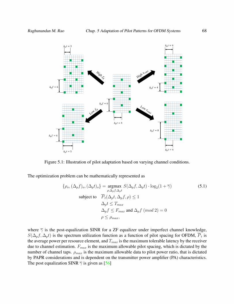
Raghunandan M. Rao Chap. 5 Adaptation of Pilot Patterns for OFDM Systems 68
Δ𝑝𝑡 = 4
Δ𝑝𝑡 = 4
Δ𝑝𝑡 = 4
Δ𝑝𝑡 = 5
Δ𝑝𝑡 = 3
Δ𝑝𝑓 = 6
Δ𝑝𝑓 = 6
Δ𝑝𝑓 = 6
Δ𝑝𝑓 = 8
Δ𝑝𝑓 = 4
Figure 5.1: Illustration of pilot adaptation based on varying channel conditions.
The optimization problem can be mathematically represented as
ρo, (∆pf)o, (∆pt)o = argmaxρ,∆pf,∆pt
S(∆pf,∆pt) · log2(1 + γ) (5.1)
subject to P t(∆pt,∆pf, ρ) ≤ 1
∆pt ≤ Tmax
∆pf ≤ Fmax and ∆pf (mod 2) = 0
ρ ≤ ρmax,
where γ is the post-equalization SINR for a ZF equalizer under imperfect channel knowledge,S(∆pf,∆pt) is the spectrum utilization function as a function of pilot spacing for OFDM, P t isthe average power per resource element, and Tmax is the maximum tolerable latency by the receiverdue to channel estimation. Fmax is the maximum allowable pilot spacing, which is dictated by thenumber of channel taps. ρmax is the maximum allowable data to pilot power ratio, that is dictatedby PAPR considerations and is dependent on the transmitter power amplifier (PA) characteristics.The post equalization SINR γ is given as [56]
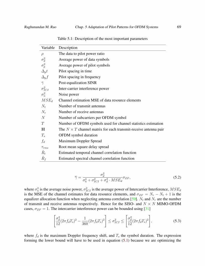
Raghunandan M. Rao Chap. 5 Adaptation of Pilot Patterns for OFDM Systems 69
Table 5.1: Description of the most important parameters
Variable Descriptionρ The data to pilot power ratioσ2d Average power of data symbolsσ2p Average power of pilot symbols
∆pt Pilot spacing in time∆pf Pilot spacing in frequencyγ Post-equalization SINRσ2ICI Inter-carrier interference powerσ2n Noise powerMSEd Channel estimation MSE of data resource elementsNt Number of transmit antennasNr Number of receive antennasN Number of subcarriers per OFDM symbolT Number of OFDM symbols used for channel statistics estimationH The N × T channel matrix for each transmit-receive antenna pairTs OFDM symbol durationfd Maximum Doppler Spreadτrms Root mean square delay spreadRt Estimated temporal channel correlation functionRf Estimated spectral channel correlation function
γ =σ2d
σ2n + σ2
ICI + σ2d ·MSEd
σZF , (5.2)
where σ2n is the average noise power, σ2
ICI is the average power of Intercarrier Interference, MSEdis the MSE of the channel estimates for data resource elements, and σZF = Nr − Nt + 1 is theequalizer allocation function when neglecting antenna correlation [59]. Nt and Nr are the numberof transmit and receive antennas respectively. Hence for the SISO- and N × N MIMO-OFDMcases, σZF = 1. The intercarrier interference power can be bounded using [31][
σ2d
12(2πfdTs)
2 − 1
360(2πfdTs)
2
]≤ σ2
ICI ≤
[σ2d
12(2πfdTs)
2
], (5.3)
where fd is the maximum Doppler frequency shift, and Ts the symbol duration. The expressionforming the lower bound will have to be used in equation (5.1) because we are optimizing the

Raghunandan M. Rao Chap. 5 Adaptation of Pilot Patterns for OFDM Systems 70
upper bound on the constrained channel capacity. The MSE for data resource elements MSEd canbe obtained by ignoring the contribution from pilots in equation (2.28) to get
MSEd =2
NB − 2
[MSE1,l
C1
+MSE2,l
C2
+ (L− 1) ·MSEf,A
]. (5.4)
The spectral utilization function depends on the number of data resource elements Nd and pilotsNp, which in turn depend on the pilot spacing ∆pt and ∆pf . For N subcarriers per OFDM symbolwith the diamond-shaped pilot arrangement, there will be Nf1 and Nf2 pilots in alternate pilot-bearing OFDM symbols. Therefore Np = Nf1 +Nf2 where Nf1 = dN/∆pe and
Nf2 =
dN/∆pfe if N (mod ∆pf) > ∆pf/2
bN/∆pfc if N (mod ∆pf) ≤ ∆pf/2,
and d.e and b.c refer to the ceiling and floor operations. The spectrum utilization function is givenas
S(∆pf,∆pt) =Nd
Nd +Np
, (5.5)
where Nd can be obtained by seeing that among N = (2 ·N ·∆pt) resource elements, Np of themare occupied by pilots. If it is a MIMO system, then RE nulls would be necessary to transmit pilotfrom other antennas, as shown in Figure 3.9 of chapter 3. Therefore, for a Nt×Nr MIMO system,Nd = (2 ·N ·∆pt−Nt ·Np) and
S(∆pf,∆pt) =2N∆pt−Nt · (Nf1 −Nf2)
2N∆pt. (5.6)
When we have a constraint on the average unit power per resource element, we have that Ndσ2d +
Npσ2p = 2N∆pt = Ntot. For a fixed ρ, the data and pilot powers can be obtained as
σ2d =
Ntot
Np/ρ+Nd
(5.7)
σ2p =
Ntot
Np + ρNd
. (5.8)
The only quantity left that is necessary to compute the upper bound of the constrained capacity isthe channel estimation MSE. The next subsection describes a method to compute MSEd.

Raghunandan M. Rao Chap. 5 Adaptation of Pilot Patterns for OFDM Systems 71
5.2.2 Estimation of Channel Statistics
To compute the MSE for data, the receiver needs the second order channel statistics Rt(∆t) andRf (∆f). In the absence of feedback, the receiver would need to estimate the channel statisticsRt(∆t) and Rf (∆f) on its own, which can be done by temporal averaging assuming local sta-tionarity of the channel for the averaging duration [60]. For a N × T channel matrix H with Nrows corresponding to frequency subcarriers, and T columns corresponding to OFDM symbols,the statistics can be estimated using
Rt(−i) =1
T − |i|
T−|i|∑t=1
diagi
[HHH
]t
Rf (−j) =1
N − |j|
N−|j|∑f=1
diagj
[HHH
]f, (5.9)
where diagi[X] is the vectorized ith diagonal of matrix X anddiagi[X]
k
its kth element. Be-
cause HHH and HHH are Hermitian-symmetric matrices, the other elements can be found usingRt(−i) = R∗t (i) and Rf (−j) = R∗f (j), where (.)∗ denotes the complex conjugate operation. Thisfollows from the properties of Hermitian symmetric matrices.
In practical scenarios where the channel statistics are estimated over a finite duration of time, theaccuracy will be poor. This occurs due to (a) interpolation error, and (b) addition of noise. In theworst case, the estimated channel statistics can violate the properties of an autocorrelation function.This is probably especially in high noise, low mobility and/or flat fading scenarios. Hence, utilizingthese estimated channel statistics directly can result in inconsistent and, sometimes absurd valuesfor the MSE. To overcome these limitations, we opt for a codebook-based approach where thereceiver stores the power delay profile and maximum Doppler Frequency values of typical channelsit expects to encounter. A cognitive radio can update the codebook over time as it learns more aboutits channel environment. The receiver calculates the channel estimates using equation (5.9) for afinite duration of time and fits it to a channel profile that best matches the estimated statistics.
5.2.3 Channel Statistics Codebook
Let the codebook be denoted by set RC with 2 disjoint subsets RC,t ⊆ RC and RC,f ⊆ RC , with|RC,f | = Mf and |RC,t| = Mt. RC,f is the set of channel frequency correlation profiles, withelements Rfc,l ∈ RC,f for 1 ≤ l ≤ Mf . Likewise, RC,t is the set of channel temporal correlationprofiles, with elements Rtc,m ∈ RC,t for 1 ≤ m ≤Mt. Here, assuming a classic Doppler spectrumRtc,m(∆t) = J0(2πfd,m∆t) from equation (2.8), where fd,m is the maximum Doppler spread forthe mth channel temporal correlation profile. Such a definition of the codebook channel profiles ismotivated by the WSSUS approximation.

Raghunandan M. Rao Chap. 5 Adaptation of Pilot Patterns for OFDM Systems 72
Initially, the profiles that comprise the codebook would correspond to the most common type ofchannels that the wireless radios would be expected to encounter, based on reported field measure-ments in the literature. Examples would be the channel profiles from ITU-T [61] and the 3GPPchannel models [62]. In the case of a cognitive radio, these profiles can be updated over time, whenit learns more about its operating environment. The codebook can be designed to match the typicalscenarios encountered, for e.g. vehicular to vehicular networks would have a large variation inDoppler spreads due to vehicular movement, UAV to UAV systems might have very low root meansquare delay spread due to strong line of sight.
5.2.4 Optimal Pilot Spacing and Power
We assume that both transmitter and receiver know and share a common P ,Df and Dt, the setsthat contain allowable values for ρ,∆pf and ∆pt, respectively. With the bounds for each parameterpredefined, the algorithm to find the optimal pilot spacing and power can be applied for everyNOFDM symbols as shown in Algorithm 1. This algorithm is executed once using the most recentNOFDM symbols. Upon its completion, it uses the subsequent NOFDM symbols for the next cycleof pilot adaptation, and so on.
Algorithm 1 Optimal pilot spacing and power allocation using codebook of channel profiles.
1: Estimate channel statistics Rt and Rf from equation (5.9) using channel estimates from themost recent NOFDM OFDM symbols across N subcarriers.
2: Find the frequency and time domain channel profiles from the codebook, Rfc,l′ and Rtc,m′
closest to the estimated statistics by evaluating
l′ = arg min1≤l≤Mf
E|Rf −Rfc,l|2
m′ = arg min1≤m≤Mt
E|Rt −Rtc,m|2. (5.10)
ForNt×Nr MIMO-OFDM, there will beNt ·Nr channel matrices of dimensionN×NOFDM .If l′ and m′ represent the NtNr × 1 vectors of codebook indices found using equation (5.10),then l′ = mode(l′),m′ = mode(m′). Here, mode(.) represents the ‘mode’ operation.
3: For ρ ∈ P ,∆pf ∈ Df ,∆pt ∈ Dt, compute channel estimation MSE MSEd assuming channelstatistics Rfc,l′ and Rtc,m′ using equation (5.4).
4: Using the values of MSE for each tuple ρ,∆tf,∆tt, solve the optimization problem bysolving equation (5.10) by calculating all the other necessary terms using equations (5.2)-(5.8).Let the resulting optimal tuple be ρo, (∆pf)o, (∆pt)o.
5: Feed back ρo, (∆pf)o, (∆pt)o to the transmitter.6: End.

Raghunandan M. Rao Chap. 5 Adaptation of Pilot Patterns for OFDM Systems 73
5.2.5 Complexity
5.2.5.1 SISO and MIMO-OFDM systems
Based on the above algorithm for pilot adaptation, the receiver needs to feed back the indices of thecorresponding channel profile from the codebook. There are a total of MtMf possible values thatcan be sent to the transmitter. Therefore, the receiver would need to feed back bf = dlog2(MtMf )ebits. Estimation of channel statistics involve matrix multiplication, which can be accomplishedwith a complexity of O(N2T ) for Rf , and O(T 2N) for Rt. Values chosen for T and N have tobe chosen to fit the statistics from the codebook more accurately. If we only need N∆t terms ofRt and N∆f terms of Rf , then the complexity becomes O(T 2N∆f ) and O(N2N∆t). Here Rt andRf will be computed by summing along the central N∆f and N∆t diagonals respectively. Sincethese operations are similar to those used in an MMSE receiver [23], its implementation does notconsume additional computing resources in modern wireless receivers.
5.2.5.2 Multi-Band Carrier Aggregation
In non-contiguous carrier aggregation, the resource blocks can be allocated to a user across two ormore frequency bands. In such a case, pilots will be sent on all Nb allocated bands (f1, f2, · · · fNb
)and the pilot spacing can be varied on each frequency band based on its channel statistics. In thiscase, some of the properties of Doppler spread can be exploited to reduce the computation andfeedback requirements for the channel profile in the codebook. We assume that the OFDM symbolduration, subcarrier spacing and all other parameters except for the pilot spacing and power, arethe same across all frequency bands. Since the Doppler frequency scales linearly with the centerfrequency fc, only 1 codebook index specifying the temporal pilot spacing needs to be fed backfor any one of the Nb bands. The temporal codebook index m′ for the other Nb − 1 bands canbe estimated at the receiver by back calculations using equations (2.8) and (5.1) - (5.8). Even inthe case when each frequency band experience different root mean square delay spreads, the totalnumber of bits needed for feedback will be b′f = dlog2(MtMf + (Nb − 1) ×Mf )e. Hence with
this method, at least log2
(NbMtMf
MtMf+(Nb−1)×Mf
)bits of feedback can be saved.
5.3 Numerical Results
This section presents the numerical simulation results showing the gains of adaptive pilot spacingand power. The two important channel statistics descriptors are the root mean square delay spreadτrms and the Doppler spread fd. Figure 5.2 shows the variation of these two parameters over timeand corresponds to the channel scenario chosen to test the performance of Algorithm 1. The rangeof parameters are 25 ns ≤ τrms ≤ 1µs and 4 Hz ≤ fd ≤ 980 Hz. For a duration of 100 ms,we assume stationarity of the channel statistics. For a total scenario duration of about 160 s, the

Raghunandan M. Rao Chap. 5 Adaptation of Pilot Patterns for OFDM Systems 74
Table 5.2: Codebook of Channel Profiles,RC
A: Channel profiles for Doppler Spread (RC,t)
Codebook Mobility Type/Velocity f †d (Hz)Index (m)
1 Pedestrian (3km/hr) 5.62 Urban Vehicular (32km/hr) 603 Highway Vehicular (120km/hr) 222.224 High Speed Train/UAV low (300km/hr) 555.565 High Speed Train/UAV medium (400km/hr) 7506 High Speed Train/UAV high (500km/hr) 925
B: Channel profiles for Frequency Selectivity (RC,f )
Codebook Normalized PDP Delay taps* τrms (ns)Index (l)
1 [0.9310, 0.3425, 0.126] [0,1,2] 221.52 [0.8882, 0.3152, 0.2809, 0.158, 0.0888] [0,1,2,3,5] 476.43 [0.778, 0.4426, 0.3097, 0.3169, 0.0497] [0,1,2,4,7] 791.24 [0.5795, 0.4745, 0.3885, 0.318, 0.2604, [0,1,2,3,4,5,6,7,8,9] 1440
0.213, 0.1745, 0.143, 0.117, 0.096]*Normalized tap coefficients for a sampling duration of Ts = 520.833 ns.† For a center frequency of fc = 2GHz.
following cases are evaluated for SISO- and 4× 4 MIMO-OFDM cases:
(a) Adaptive pilot spacing and power, 2 ≤ ∆pt ≤ 10, 2 ≤ ∆pf ≤ 8,−8 dB ≤ ρ ≤ 0 dB.
(b) LTE Pilot spacing as shown in Figure 4.1, ρ = −3 dB.
(c) Fixed pilot spacing and power, ∆pt = 6,∆pf = 6, ρ = −3 dB.
(d) Fixed pilot spacing and power, ∆pt = 8,∆pf = 8, ρ = −3 dB.
The diamond-shaped pilot patterns shown in Figure 3.9 are used for simulation of 4 × 4 MIMO-OFDM with full-rank spatial multiplexing. The other simulation parameters are presented in Table2.2. We have used QPSK modulation on each data subcarrier of the OFDM symbol. For eachcase, the channel parameters τrms and fd were held constant for NOFDM = 1500 OFDM symbols.Using Algorithm 1, the channel scenario for case (a) was simulated using the codebook of Table5.2.
Raghunandan M. Rao Chap. 5 Adaptation of Pilot Patterns for OFDM Systems 75
5.3.0.1 Performance of Pilot Adaptation in SISO-OFDM
Figure 5.3 shows the ergodic capacity versus SNR for all considered pilot configurations (a)-(d).We see that pilot adaptation outperforms the other configurations for almost all values of SNR.We also see that the increase in channel capacity of pilot adaptation w.r.t. other fixed configurationsimproves with increasing Eb/N0. This can be attributed to better estimation of channel statisticswith higher SNR values. Figure 5.5 shows the channel capacity gain achieved by adapting pilotspacing and power. The capacity gain w.r.t. LTE spacing saturates at ∼ 10% for higher valuesof SNR. The capacity gain w.r.t. other pilot configuration shows an almost linear increase withSNR.
Figure 5.4 shows the comparison of Cumulative Distribution Function (CDF) FC(Cs) of the ca-pacity C for pilot adaptation versus LTE spacing. The CDF is given by
FC(Cs) = P[C ≤ Cs] (5.11)
where P[X ≤ x] is the probability that the random variable X is less than or equal to x. We seethat there is a significant performance improvement in the CDF, even at low SNR values. The non-existence of crossovers between the Cumulative Distribution Functions (CDFs) of the capacities ofpilot adaptation and LTE spacing cases implies the achievability of throughput improvement usingpilot adaptation under all operating conditions. The first three rows of Table 5.3 shows the averageperformance improvement of adaptive pilot configurations over the fixed pilot configurations.
5.3.0.2 Performance of Pilot Adaptation in MIMO-OFDM
Figure 5.6 shows the achievable ergodic capacity versus SNR for all the simulated pilot configura-tions for MIMO-OFDM. Similar to the case in SISO, we see that our pilot adaptation algorithm out-performs all fixed pilot configurations. Figure 5.7 shows the CDF of capacity for pilot pattern adap-tation versus LTE spacing. We see that pilot pattern adaptation outperforms the LTE pilot patternin all operating conditions. The capacity gains w.r.t. fixed pilot configurations is shown in Figure5.8, where we see the capacity gains w.r.t. LTE spacing saturates at∼ 20%. This behavior is likelybecause of the error floor introduced by the channel estimation algorithm in relatively fast fadingand high τrms channel environments. Moreover, the matrix inversion operations in ZF receiverscan result in relatively higher noise enhancement for fast fading scenarios even at high SNR values.This is seen as a clustering of the tail of the capacity CDF at SNR = 13 dB and SNR = 28 dB.The last three rows of Table 5.3 summarize the capacity gains of pilot adaptation.
5.3.0.3 Variation of Capacity Gain with SNR
In Figures 5.5 and 5.8, we observe that the throughput gain of pilot adaptation w.r.t. that of LTEis not monotonically increasing as a function of the SNR. On the other hand, the throughput gain
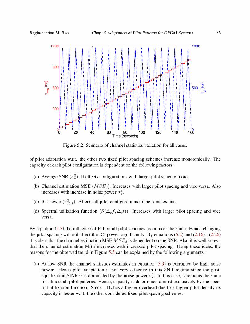
Raghunandan M. Rao Chap. 5 Adaptation of Pilot Patterns for OFDM Systems 76
0 20 40 60 80 100 120 140 1600
300
600
900
1200
Time (seconds)
τrm
s (
ns)
0 20 40 60 80 100 120 1400
500
1000
f d (
Hz)
Figure 5.2: Scenario of channel statistics variation for all cases.
of pilot adaptation w.r.t. the other two fixed pilot spacing schemes increase monotonically. Thecapacity of each pilot configuration is dependent on the following factors:
(a) Average SNR (σ2n): It affects configurations with larger pilot spacing more.
(b) Channel estimation MSE (MSEd): Increases with larger pilot spacing and vice versa. Alsoincreases with increase in noise power σ2
n.
(c) ICI power (σ2ICI): Affects all pilot configurations to the same extent.
(d) Spectral utilization function (S(∆pf,∆pt)): Increases with larger pilot spacing and viceversa.
By equation (5.3) the influence of ICI on all pilot schemes are almost the same. Hence changingthe pilot spacing will not affect the ICI power significantly. By equations (5.2) and (2.16) - (2.26)it is clear that the channel estimation MSE MSEd is dependent on the SNR. Also it is well knownthat the channel estimation MSE increases with increased pilot spacing. Using these ideas, thereasons for the observed trend in Figure 5.5 can be explained by the following arguments:
(a) At low SNR the channel statistics estimates in equation (5.9) is corrupted by high noisepower. Hence pilot adaptation is not very effective in this SNR regime since the post-equalization SINR γ is dominated by the noise power σ2
n. In this case, γ remains the samefor almost all pilot patterns. Hence, capacity is determined almost exclusively by the spec-tral utilization function. Since LTE has a higher overhead due to a higher pilot density itscapacity is lesser w.r.t. the other considered fixed pilot spacing schemes.

Raghunandan M. Rao Chap. 5 Adaptation of Pilot Patterns for OFDM Systems 77
0 5 10 15 20 25 301
2
3
4
5
6
7
8
SNR (dB)
Erg
od
ic C
ap
acity (
bp
s/H
z)
Pilot spacing and power adaptation
LTE spacing, ρ = −3dB
∆p t = 6, ∆
p f = 6, ρ = −3dB
∆p t = 8, ∆
p f = 8, ρ = −3dB
Figure 5.3: Ergodic Capacity Performance in SISO-OFDM for all considered pilot configurations.
0 2 4 6 8 10 120
0.1
0.2
0.3
0.4
0.5
0.6
0.7
0.8
0.9
1
Capacity (bps/Hz)
CD
F o
f C
apacity
Pilot adaptation, SNR = 3dB
Pilot adaptation, SNR = 13dB
Pilot adaptation, SNR = 28dB
LTE Spacing, ρ = −3dB, SNR = 3dB
LTE Spacing, ρ = −3dB, SNR = 13dB
LTE Spacing, ρ = −3dB, SNR = 28dB
Figure 5.4: The CDF of Capacity for pilot adaptation versus LTE spacing, ρ = −3 dB for SISO-OFDM.
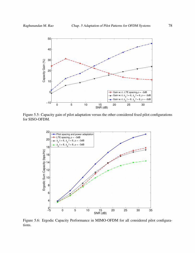
Raghunandan M. Rao Chap. 5 Adaptation of Pilot Patterns for OFDM Systems 78
0 5 10 15 20 25 30−10
0
10
20
30
40
50
Capacity G
ain
(%
)
SNR (dB)
Gain w.r.t. LTE spacing, ρ = −3dB
Gain w.r.t. ∆p t = 6, ∆
p f = 6, ρ = −3dB
Gain w.r.t. ∆p t = 8, ∆
p f = 8, ρ = −3dB
Figure 5.5: Capacity gain of pilot adaptation versus the other considered fixed pilot configurationsfor SISO-OFDM.
−5 0 5 10 15 20 25 30 352
4
6
8
10
12
14
16
18
20
22
SNR (dB)
Erg
od
ic S
um
Ca
pa
city (
bp
s/H
z)
Pilot spacing and power adaptation
LTE spacing, ρ = −3dB
∆p t = 6, ∆
p f = 6, ρ = −3dB
∆p t = 8, ∆
p f = 8, ρ = −3dB
Figure 5.6: Ergodic Capacity Performance in MIMO-OFDM for all considered pilot configura-tions.
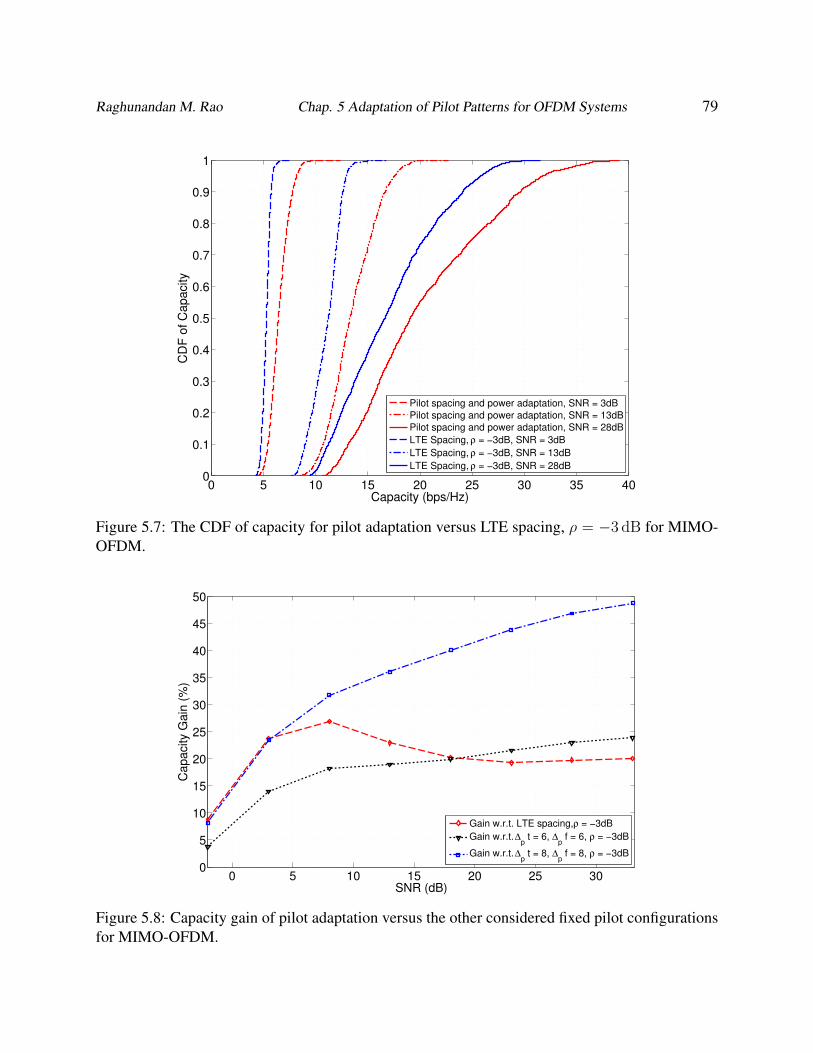
Raghunandan M. Rao Chap. 5 Adaptation of Pilot Patterns for OFDM Systems 79
0 5 10 15 20 25 30 35 400
0.1
0.2
0.3
0.4
0.5
0.6
0.7
0.8
0.9
1
Capacity (bps/Hz)
CD
F o
f C
apacity
Pilot spacing and power adaptation, SNR = 3dB
Pilot spacing and power adaptation, SNR = 13dB
Pilot spacing and power adaptation, SNR = 28dB
LTE Spacing, ρ = −3dB, SNR = 3dB
LTE Spacing, ρ = −3dB, SNR = 13dB
LTE Spacing, ρ = −3dB, SNR = 28dB
Figure 5.7: The CDF of capacity for pilot adaptation versus LTE spacing, ρ = −3 dB for MIMO-OFDM.
0 5 10 15 20 25 300
5
10
15
20
25
30
35
40
45
50
Ca
pa
city G
ain
(%
)
SNR (dB)
Gain w.r.t. LTE spacing, ρ = −3dB
Gain w.r.t. ∆p t = 6, ∆
p f = 6, ρ = −3dB
Gain w.r.t. ∆p t = 8, ∆
p f = 8, ρ = −3dB
Figure 5.8: Capacity gain of pilot adaptation versus the other considered fixed pilot configurationsfor MIMO-OFDM.
Raghunandan M. Rao Chap. 5 Adaptation of Pilot Patterns for OFDM Systems 80
(b) With increasing SNR the other factors begin to contribute to the capacity. On one handthe capacity improvements due to pilot adaptation begins to increase with increase in SNR.As the σ2
n value decreases the contribution of MSEd term begins to dominate for all pilotspacing configurations. For LTE spacing its low spectral utilization decreases its capacityas compared to the other fixed pilot schemes. But as SNR increases, the other fixed pilotschemes begin to perform worse due to increasing MSEd and their high spectral utilizationbecomes ineffective. Hence LTE eventually outperforms these schemes for SNR ≥ 20 dB.
(c) For high values of SNR, MSEd is dominated by the temporal and spectral channel corre-lation terms due to fading. At the same time the contribution of noise power σ2
n on MSEdbegins to decrease with increasing SNR. Therefore channel fading and ICI determines thecapacity in this regime and pilot adaptation works accurately to track changes in the channelstatistics. Since closer pilot spacing yields a lesser MSEd value, LTE performs better whilethe other fixed pilot schemes lose capacity due to increased MSEd.
(d) The capacity gain of pilot adaptation w.r.t. LTE spacing begins to saturate as SNR goes be-yond 20 dB. This is because the capacity begins to saturate in both LTE and pilot adaptationdue to MSEd, which does not depend on SNR in this regime. In other words, LTE spac-ing is close to the optimal pilot spacing for typical mobile wireless channels in high SNRconditions.
For the case of 4 × 4 MIMO-OFDM with full rank spatial multiplexing we see a similar trendin the capacity gains in Figure 5.8 as we do in the case of SISO-OFDM. Most of the argumentsput forth above hold true here as well. However the performance of LTE spacing with that of the∆pt = ∆pf = 8, ρ = −3 dB case is similar at low SNR. This behavior is due to the fact that thechannel estimation errors MSEd accumulates on all 16 channel estimates (one channel estimatefor each transmit-receive antenna pair) of the channel matrix H in equation (3.7). Hence the errordue to MSEd does not become negligible for very large pilot spacing.
However, it is clear that pilot adaptation outperforms all fixed pilot schemes as it balances channelestimation performance and pilot overhead for a wide range of channel fading statistics and noiseconditions.
5.3.0.4 Comparison with the State of the Art
The authors in [56] have compared the performance of their pilot adaptation algorithm w.r.t. thatof LTE. They have mapped each pilot pattern to a CQI value of LTE. Therefore, a flat fadingchannel in their case will result in (a) throughput gain due to overhead reduction of pilots, and (b)throughput scaling due to increased spectral efficiency as a result of higher modulation order (referto Table 4.1). It is to be noted that:
1. They have considered data throughput as a metric for comparison, whereas we have consid-ered ergodic capacity as a metric in order to compare our algorithm’s performance versus
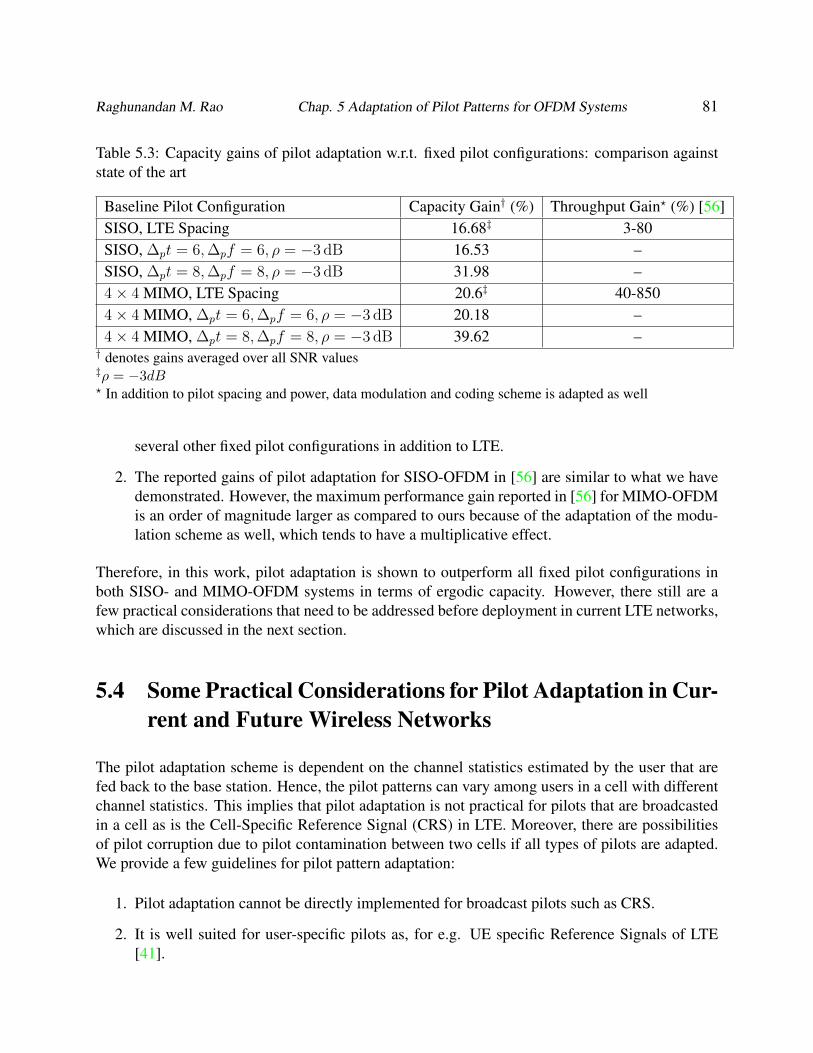
Raghunandan M. Rao Chap. 5 Adaptation of Pilot Patterns for OFDM Systems 81
Table 5.3: Capacity gains of pilot adaptation w.r.t. fixed pilot configurations: comparison againststate of the art
Baseline Pilot Configuration Capacity Gain† (%) Throughput Gain? (%) [56]SISO, LTE Spacing 16.68‡ 3-80SISO, ∆pt = 6,∆pf = 6, ρ = −3 dB 16.53 –SISO, ∆pt = 8,∆pf = 8, ρ = −3 dB 31.98 –4× 4 MIMO, LTE Spacing 20.6‡ 40-8504× 4 MIMO, ∆pt = 6,∆pf = 6, ρ = −3 dB 20.18 –4× 4 MIMO, ∆pt = 8,∆pf = 8, ρ = −3 dB 39.62 –† denotes gains averaged over all SNR values‡ρ = −3dB? In addition to pilot spacing and power, data modulation and coding scheme is adapted as well
several other fixed pilot configurations in addition to LTE.
2. The reported gains of pilot adaptation for SISO-OFDM in [56] are similar to what we havedemonstrated. However, the maximum performance gain reported in [56] for MIMO-OFDMis an order of magnitude larger as compared to ours because of the adaptation of the modu-lation scheme as well, which tends to have a multiplicative effect.
Therefore, in this work, pilot adaptation is shown to outperform all fixed pilot configurations inboth SISO- and MIMO-OFDM systems in terms of ergodic capacity. However, there still are afew practical considerations that need to be addressed before deployment in current LTE networks,which are discussed in the next section.
5.4 Some Practical Considerations for Pilot Adaptation in Cur-rent and Future Wireless Networks
The pilot adaptation scheme is dependent on the channel statistics estimated by the user that arefed back to the base station. Hence, the pilot patterns can vary among users in a cell with differentchannel statistics. This implies that pilot adaptation is not practical for pilots that are broadcastedin a cell as is the Cell-Specific Reference Signal (CRS) in LTE. Moreover, there are possibilitiesof pilot corruption due to pilot contamination between two cells if all types of pilots are adapted.We provide a few guidelines for pilot pattern adaptation:
1. Pilot adaptation cannot be directly implemented for broadcast pilots such as CRS.
2. It is well suited for user-specific pilots as, for e.g. UE specific Reference Signals of LTE[41].
Raghunandan M. Rao Chap. 5 Adaptation of Pilot Patterns for OFDM Systems 82
3. It is also applicable for peer-to-peer links such as wireless backhaul, vehicular to vehicu-lar, UAV to ground/UAV to UAV systems. In such systems, interference with other pilotstypically does not arise.
4. Approaches like grouping of users having similar channel conditions during resource al-location [63] or active user-aware dynamic pilot distribution would be starting points foradaptation of broadcast pilots.
5.5 Conclusions
In this chapter, we developed a simple codebook-based algorithm to adapt the pilot spacing andpower in SISO- and MIMO-OFDM systems. Using pilot adaptation, we demonstrated a channelcapacity gain of about 10-30% for SISO, and 10-27% for 4×4 MIMO-OFDM w.r.t. the fixed LTEpilot configuration. Monte-Carlo simulations showed that pilot adaptation outperforms all fixedpilot configurations for almost all SNR values in a non-stationary wireless channel with smoothlyvarying channel statistics. We also discussed a scheme to reduce the channel statistics feedbackrequirements for inter-band carrier aggregation systems.
A ten-fold increase in spectral efficiency is expected to be necessary to meet the traffic demandsof future 5G networks. Pilot pattern adaptation alone has the potential to enhance the spectralefficiency by 1.5 − 2× (excluding the effects of adaptive modulation and coding), which is anecessary first step to reduce overhead in the transport blocks of current wireless networks.
Chapter 6
Conclusions and Future Work
6.1 Thesis Summary and Conclusions
This thesis investigated the role of pilot signals in the evolution of wireless networks. We focusedon the resilience of pilots to targeted interference and on optimizing its density to maximize chan-nel capacity as a function of the channel conditions in the absence of targeted interference. Wealso experimented with the LTE downlink to study its robustness to targeted interference on theCRS (downlink pilot signals) and, to the best of our knowledge, demonstrated the ‘CQI spoofingattack’ in LTE for the first time. The key conclusions of this thesis are outlined below.
In Chapter 2, we provided theoretical expressions for BER and channel estimation MSE, both inthe presence as well as absence of a multi-tone pilot jammer. We estimated that multi-tone pilotjamming has the potential to disrupt communications by transmitting about 9 dB less power thanthe target signal if synchronized perfectly with its target (for pilot densities similar to the onesused in LTE). The theoretical and simulated performance was found to be very close to each other,validating the accuracy of our simulator.
In Chapter 3, we proposed and evaluated methods to counter a pilot jammer in both SISO- andMIMO-OFDM scenarios. For SISO-OFDM it was seen that for an asynchronous pilot jammer,there was an improvement in the channel estimation performance. To improve the BER perfor-mance, complementary methods such Adaptive Modulation and Coding, Hybrid ARQ are neces-sary. For MIMO-OFDM, we explored whether full rank spatial-multiplexing operation is possiblein the presence of a synchronous power-constrained pilot jammer. We devised a simple cancella-tion scheme for such jammers by exploiting the channel flatness in either the time or frequencydimensions to cancel out the interference. We demonstrated that such cancellation can achieve∼ 50 − 90% of the interference-free ergodic sum capacity in 4 × 4 MIMO with full rank spatialmultiplexing.
In Chapter 4, we demonstrated the problem of ‘CRS Jamming’ and ‘CQI Spoofing’ in the LTE
83
Raghunandan M. Rao Chap. 6 Conclusions and Future Work 84
Downlink. Our RF measurements with 3GPP-compliant LTE test systems showed that CRS Jam-ming required ∼ 5 dB less power than Barrage Jamming to cause DoS at the UE. Pilot jammerevasion by cyclic shifting of pilot locations proved to be ineffective due to the inability of the UEto track the channel quality correctly. We have identified this to be a problem as severe as ‘CRSJamming’ and conclude that further research on accurate CQI estimation/correction algorithms inthe presence of targeted interference is necessary.
Finally in Chapter 5, we investigated the idea of pilot pattern adaptation in SISO- and MIMO-OFDM systems. We developed a simple codebook-based approach to adapt the pilot spacing andpower in SISO- and MIMO-OFDM systems, which demonstrated a channel capacity gain of about10-30 % for SISO, and 10-27% for 4 × 4 MIMO-OFDM w.r.t. the fixed LTE pilot configuration.Monte-Carlo simulations showed that pilot adaptation outperforms all fixed pilot configurationsfor almost all SNR values in nonstationary channels with smoothly varying channel statistics. Wealso discussed some practical constraints that need to be addressed before pilot adaptation can beimplemented into current and future wireless standards.
6.2 Future Work
There can be several extensions to this work, some of which are categorized below.
6.2.1 Enhanced Mitigation Algorithms for Pilot Jamming
In this work, we have considered a power-constrained jammer that reduces its symbol rate w.r.t. thetarget signal to localize most of its power on pilot subcarriers. Mitigation strategies are necessaryto deal with jammers which transmit at the same symbol rate as the target OFDM symbol. In thiscase, the jammer needs to be closely tracked in every symbol duration. This will prove useful tomake the pilot signals more resilient against jamming.
In addition, jamming of uplink pilots in schemes like Single Carrier-Frequency Division Multi-ple Access (SC-FDMA) will also be a worthwhile effort, especially considering the fact that thereceived power of the uplink signal will always be order of magnitudes lower than that of thedownlink signal.
6.2.2 Improving Resilience of LTE
This work specifically focused on the resilience of pilots to targeted interference in LTE. An im-mediate problem to be fixed in LTE is ‘CQI Spoofing’ and development of better CQI estimationalgorithms is necessary to improve the throughput performance of LTE when the jammer explicitlyavoids interfering with pilot locations of the LTE signal.

Raghunandan M. Rao Chap. 6 Conclusions and Future Work 85
New threats will emerge with newer releases of LTE and it will be crucial to investigate the robust-ness of the LTE standard to these attacks.
6.2.3 Cross-layer Optimization in Interference Channels
Chapter 4 identified the problems caused by interference when assumptions go wrong during sys-tem design. Most CQI estimation algorithms are developed to optimize performance in frequencyselective mobile fading channels. The same algorithm causes performance degradation when in-tentional or unintentional interference is present on data subcarriers. The ramifications of thisinterference on higher layers needs more research in order to design better protocols for 5G.
6.2.4 Trust-Aware Protocol Design
The performance of each layer depends on the layers below it in the protocol stack. In currentprotocols each layer trusts the input it gets from other layers. An interesting paradigm shift wouldbe to investigate the effect of establishing different levels of trust between all layers of the proto-col, on the system performance. Incorporating trust between layers into protocol design has thepotential to mitigate undesired behavior in the presence of protocol-aware attackers.
6.2.5 Pilot Pattern Adaptation
Some constraints of pilot adaptation were highlighted in chapter 5 of this thesis. Considerableresearch effort is necessary to overcome the inherent constraints of adapting broadcast pilots. Sincebroadcast pilots comprise a major chunk of the essential overhead in the physical layer signal, itwill be interesting to see if broadcast pilot patterns can be adapted at all, using techniques like theones described in [63]. An interesting problem would be to solve the optimization problem posedin equation (5.1) in the presence of a multi-tone pilot jammer that constantly tracks changes in thepilot pattern of its target.
For 5G networks, alternate multicarrier waveforms such as Filter-bank Multicarrier (FBMC), Uni-versal Filtered Multicarrier (UFMC) [5] are being actively researched. Like other multicarrierwaveforms, pilot-aided channel estimation is the preferred method to equalize the FBMC signals[64]. Hence, algorithms to adapt pilot patterns to maximize throughput are necessary. Since theyhave different sources of interference than OFDM, it is necessary to be modeled accurately. Theformulation of the cost function that maximizes the channel capacity (or its upper bound) for allpotential waveforms would be a significant contribution to choose and optimize the PHY layer for5G.

Appendix A
Additional Throughput MeasurementResults
In chapter 4 the performance of LTE downlink in the presence of targeted interference was investi-gated. This appendix presents additional results to support our findings and conclusions in chapter4. The throughput was measured for the LTE downlink in the following scenarios:
(a) CRS jamming,
(b) Data subcarrier jamming (one out of every three subcarriers),
(c) Barrage jamming.
The measurements were carried out for four trials for each of the above scenarios. The measure-ment results are shown in Table A.1. The following parameters are shown as a function of JSR foreach case:
(a) Mean (µ) of measured throughput Rmeas,
(b) Standard deviation (σ) of measured throughput Rmeas,
(c) Median value of the reported Modulation and coding scheme (MCS).
An important takeaway from this table is the reported median MCS values for data subcarrierjamming. A high value of MCS in the presence of targeted interference results in a higher numberof errors that reduces the throughput. Hence accurate CQI estimation algorithms are necessary tooptimize the performance in the presence of targeted interference on data subcarriers.
86
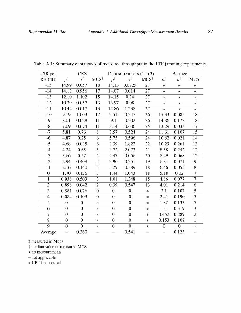
Raghunandan M. Rao Appendix A Additional Throughput Measurement Results 87
Table A.1: Summary of statistics of measured throughput in the LTE jamming experiments.
JSR per CRS Data subcarriers (1 in 3) BarrageRB (dB) µ‡ σ‡ MCS† µ‡ σ‡ MCS† µ‡ σ‡ MCS†
-15 14.99 0.057 18 14.13 0.0825 27 ? ? ?-14 14.13 0.956 17 14.07 0.014 27 ? ? ?-13 12.10 1.102 15 14.15 0.24 27 ? ? ?-12 10.39 0.057 13 13.97 0.08 27 ? ? ?-11 10.42 0.017 13 12.86 1.238 27 ? ? ?-10 9.19 1.003 12 9.51 0.347 26 15.33 0.085 18-9 8.01 0.028 11 9.1 0.202 26 14.86 0.172 18-8 7.09 0.674 11 8.14 0.406 25 13.29 0.033 17-7 5.81 0.76 8 7.57 0.524 24 11.61 0.107 15-6 4.87 0.25 6 5.75 0.596 24 10.82 0.021 14-5 4.68 0.035 6 3.39 1.822 22 10.29 0.261 13-4 4.24 0.65 5 3.72 2.073 21 8.58 0.252 12-3 3.66 0.57 5 4.47 0.056 20 8.29 0.068 12-2 2.94 0.408 4 3.90 0.351 19 6.84 0.071 9-1 2.16 0.140 3 3.29 0.389 18 6.46 0.055 80 1.70 0.126 3 1.44 1.043 18 5.18 0.02 71 0.938 0.503 3 1.01 1.348 15 4.86 0.077 72 0.898 0.042 2 0.39 0.547 13 4.01 0.214 63 0.581 0.076 0 0 0 ∗ 3.1 0.107 54 0.084 0.103 0 0 0 ∗ 2.41 0.190 55 0 0 ∗ 0 0 ∗ 1.82 0.133 56 0 0 ∗ 0 0 ∗ 1.31 0.319 37 0 0 ∗ 0 0 ∗ 0.452 0.289 28 0 0 ∗ 0 0 ∗ 0.153 0.108 19 0 0 ∗ 0 0 ∗ 0 0 ∗
Average – 0.360 – – 0.541 – – 0.123 –
‡ measured in Mbps† median value of measured MCS? no measurements– not applicable∗ UE disconnected

Bibliography
[1] S. Sesia, M. Baker, and I. Toufik, LTE-The UMTS Long Term Evolution: From Theory toPractice. John Wiley & Sons, 2011.
[2] ETSI, “LTE, Evolved Universal Terrestrial Radio Access (E-UTRA), Physical Layer Proce-dures (3GPP TS 36.213 v 12.4.0), Release 12,” 3GPP, 2015.
[3] 3GPP, “Releases,” http://www.3gpp.org/specifications/67-releases, 2016, [Online; accessed19-July-2016].
[4] J. G. Andrews, S. Buzzi, W. Choi, S. V. Hanly, A. Lozano, A. C. K. Soong, and J. C. Zhang,“What Will 5G Be?” IEEE Journal on Selected Areas in Communications, vol. 32, no. 6, pp.1065–1082, June 2014.
[5] P. Banelli, S. Buzzi, G. Colavolpe, A. Modenini, F. Rusek, and A. Ugolini, “ModulationFormats and Waveforms for 5G Networks: Who Will Be the Heir of OFDM?: An overviewof alternative modulation schemes for improved spectral efficiency,” IEEE Signal ProcessingMagazine, vol. 31, no. 6, pp. 80–93, Nov 2014.
[6] S. Schwarz and M. Rupp, “Society in motion: challenges for LTE and beyond mobile com-munications,” IEEE Communications Magazine, vol. 54, no. 5, pp. 76–83, May 2016.
[7] T. C. Clancy, “Efficient OFDM Denial: Pilot Jamming and Pilot Nulling,” in Communications(ICC), IEEE International Conference on, June 2011, pp. 1–5.
[8] C. Shahriar, R. McGwier, and T. C. Clancy, “Performance impact of pilot tone randomiza-tion to mitigate OFDM jamming attacks,” in Consumer Communications and NetworkingConference (CCNC), IEEE, Jan 2013, pp. 813–816.
[9] C. S. Patel, G. L. Stuber, and T. G. Pratt, “Analysis of OFDM/MC-CDMA under channelestimation and jamming,” in Wireless Communications and Networking Conference (WCNC),IEEE, vol. 2, March 2004, pp. 954–958 Vol.2.
[10] M. Han, T. Yu, J. Kim, K. Kwak, S. Lee, S. Han, and D. Hong, “OFDM Channel EstimationWith Jammed Pilot Detector Under Narrow-Band Jamming,” IEEE Transactions on VehicularTechnology, vol. 57, no. 3, pp. 1934–1939, May 2008.
88
Raghunandan M. Rao Bibliography 89
[11] J. A. Mahal and T. C. Clancy, “The closed-form BER expressions of PSK modulation forOFDM and SC-FDMA under jamming and imperfect channel estimation,” in Communica-tions (ICC), IEEE International Conference on, June 2014, pp. 2221–2226.
[12] C. Shahriar, T. C. Clancy, and R. W. McGwier, “Equalization attacks against OFDM: analysisand countermeasures,” Wireless Communications and Mobile Computing, pp. n/a–n/a, 2015.[Online]. Available: http://dx.doi.org/10.1002/wcm.2648
[13] C. A. Cole, C. Shahriar, and T. C. Clancy, “An Anti-jam Communications Technique viaSpatial Hiding Precoding,” in IEEE Military Communications Conference, Oct 2014, pp.490–494.
[14] G. D. Durgin, V. Kukshya, and T. S. Rappaport, “Wideband measurements of angle anddelay dispersion for outdoor and indoor peer-to-peer radio channels at 1920 MHz,” IEEETransactions on Antennas and Propagation, vol. 51, no. 5, pp. 936–944, May 2003.
[15] J. Kakar, K. McDermott, V. Garg, M. Lichtman, V. Marojevic, and J. H. Reed, “Analysis andMitigation of Interference to the LTE Physical Control Format Indicator Channel,” in IEEEMilitary Communications Conference, Oct 2014, pp. 228–234.
[16] M. Lichtman, T. Czauski, S. Ha, P. David, and J. H. Reed, “Detection and Mitigation ofUplink Control Channel Jamming in LTE,” in IEEE Military Communications Conference,Oct 2014, pp. 1187–1194.
[17] M. Labib, V. Marojevic, and J. H. Reed, “Analyzing and enhancing the resilience ofLTE/LTE-A systems to RF spoofing,” in IEEE Conference on Standards for Communicationsand Networking (CSCN), Oct 2015, pp. 315–320.
[18] M. Lichtman, R. P. Jover, M. Labib, R. Rao, V. Marojevic, and J. H. Reed, “LTE/LTE-Ajamming, spoofing, and sniffing: threat assessment and mitigation,” IEEE CommunicationsMagazine, vol. 54, no. 4, pp. 54–61, April 2016.
[19] R. P. Jover, J. Lackey, and A. Raghavan, “Enhancing the security of LTE networks againstjamming attacks,” EURASIP Journal on Information Security, vol. 2014, no. 1, pp. 1–14,2014.
[20] O. Sallent and R. Ferrs, Mobile Broadband Communications for Public Safety: The RoadAhead Through LTE Technology. John Wiley & Sons, 2015.
[21] C. Shahriar, M. L. Pan, M. Lichtman, T. C. Clancy, R. McGwier, R. Tandon, S. Sodagari, andJ. H. Reed, “PHY-Layer Resiliency in OFDM Communications: A Tutorial,” IEEE Commu-nications Surveys Tutorials, vol. 17, no. 1, pp. 292–314, First quarter 2015.
[22] T. Basar, “The Gaussian test channel with an intelligent jammer,” IEEE Transactions onInformation Theory, vol. 29, no. 1, pp. 152–157, Jan 1983.

Raghunandan M. Rao Bibliography 90
[23] M. K. Ozdemir and H. Arslan, “Channel estimation for wireless OFDM systems,” IEEECommunications Surveys Tutorials, vol. 9, no. 2, pp. 18–48, second quarter 2007.
[24] L. Jun, J. H. Andrian, and C. Zhou, “Bit Error Rate Analysis of jamming for OFDM systems,”in Wireless Telecommunications Symposium, April 2007, pp. 1–8.
[25] I. Barhumi, G. Leus, and M. Moonen, “Optimal training design for MIMO-OFDM systemsin mobile wireless channels,” IEEE Transactions on Signal Processing, vol. 51, no. 6, pp.1615–1624, June 2003.
[26] C. R. N. Athaudage and A. D. S. Jayalath, “Low-complexity channel estimation for wire-less OFDM systems,” in Personal, Indoor and Mobile Radio Communications, 14th IEEEProceedings on, vol. 1, Sept 2003, pp. 521–525.
[27] Y. Li, “Pilot-symbol-aided channel estimation for OFDM in wireless systems,” IEEE Trans-actions on Vehicular Technology, vol. 49, no. 4, pp. 1207–1215, Jul 2000.
[28] W. C. Jakes and D. C. Cox, Microwave mobile communications. Wiley-IEEE Press, 1994.
[29] R. Ratasuk, N. Mangalvedhe, A. Ghosh, and B. Vejlgaard, “Narrowband LTE-M System forM2M Communication,” in IEEE 80th Vehicular Technology Conference (VTC 2014-Fall),Sept 2014, pp. 1–5.
[30] J. Kim, J. Park, and D. Hong, “Performance analysis of channel estimation in OFDM sys-tems,” Signal Processing Letters, IEEE, vol. 12, no. 1, pp. 60–62, Jan 2005.
[31] Y. Li and L. J. Cimini, “Bounds on the interchannel interference of OFDM in time-varyingimpairments,” IEEE Transactions on Communications, vol. 49, no. 3, pp. 401–404, 2001.
[32] M.-X. Chang and Y. T. Su, “Performance analysis of equalized OFDM systems in Rayleighfading,” IEEE Transactions on Wireless Communications, vol. 1, no. 4, pp. 721–732, Oct2002.
[33] R. Nissel, M. Lerch, M. Simko, and M. Rupp, “Bit Error Probability for Pilot-Symbol-AidedOFDM Channel Estimation in Doubly-Selective Channels,” in Smart Antennas (WSA), 18thInternational ITG Workshop on, March 2014, pp. 1–6.
[34] L. C. Godara, “Application of antenna arrays to mobile communications. II. Beam-formingand direction-of-arrival considerations,” Proceedings of the IEEE, vol. 85, no. 8, pp. 1195–1245, Aug 1997.
[35] Q. H. Spencer, A. L. Swindlehurst, and M. Haardt, “Zero-forcing methods for downlinkspatial multiplexing in multiuser MIMO channels,” IEEE Transactions on Signal Processing,vol. 52, no. 2, pp. 461–471, Feb 2004.

Raghunandan M. Rao Bibliography 91
[36] Q. Yan, H. Zeng, T. Jiang, M. Li, W. Lou, and Y. T. Hou, “Jamming Resilient CommunicationUsing MIMO Interference Cancellation,” IEEE Transactions on Information Forensics andSecurity, vol. 11, no. 7, pp. 1486–1499, July 2016.
[37] S. Sodagari and T. C. Clancy, “Efficient jamming attacks on MIMO channels,” in IEEE In-ternational Conference on Communications (ICC), June 2012, pp. 852–856.
[38] S. Amuru and R. M. Buehrer, “Optimal jamming against digital modulation,” IEEE Transac-tions on Information Forensics and Security, vol. 10, no. 10, pp. 2212–2224, Oct 2015.
[39] J. G. Proakis and M. Salehi, Digital Communications. McGraw-Hill, 2007.
[40] T. Li, W. H. Mow, V. K. N. Lau, M. Siu, R. S. Cheng, and R. D. Murch, “Robust jointinterference detection and decoding for OFDM-based cognitive radio systems with unknowninterference,” IEEE Journal on Selected Areas in Communications, vol. 25, no. 3, pp. 566–575, April 2007.
[41] ETSI, “LTE, Evolved Universal Terrestrial Radio Access (E-UTRA), Requirements for sup-port of radio resource management (3GPP TS 36.133 v 10.1.0), Release 10,” 3GPP, 2011.
[42] ——, “LTE, Evolved Universal Terrestrial Radio Access (E-UTRA), Physical Channels andModulation (3GPP TS 36.211 v 9.1.0), Release 9,” 3GPP, 2010.
[43] H. Yang, A. Huang, R. Gao, T. Chang, and L. Xie, “Interference Self-Coordination: A Pro-posal to Enhance Reliability of System-Level Information in OFDM-Based Mobile Networksvia PCI Planning,” IEEE Transactions on Wireless Communications, vol. 13, no. 4, pp. 1874–1887, April 2014.
[44] A. Paulraj, R. Nabar, and D. Gore, Introduction to Space-time Wireless Communications.Cambridge University Press, 2003.
[45] F. Boccardi, R. W. Heath, A. Lozano, T. L. Marzetta, and P. Popovski, “Five disruptive tech-nology directions for 5G,” IEEE Communications Magazine, vol. 52, no. 2, pp. 74–80, Febru-ary 2014.
[46] S. Amuru, “Intelligent Approaches for Communication Denial,” Ph.D. dissertation, VirginiaTech, September 2015.
[47] M. Simko, “Pilot Pattern Optimization for Doubly-Selective MIMO OFDM Transmissions,”Ph.D. dissertation, Vienna University of Technology, May 2013.
[48] T. Doumi, M. F. Dolan, S. Tatesh, A. Casati, G. Tsirtsis, K. Anchan, D. Flore, “LTE for PublicSafety Networks,” Communications Magazine, IEEE, vol. 51, no. 2, pp. 106–112, 2013.
[49] “Amarisoft LTE100,” http://amarisoft.com/document/Amarisoft LTE100.pdf, 2016, [Online;last accessed 14-July-2016].

Raghunandan M. Rao Bibliography 92
[50] “GNURadio,” http://gnuradio.org/, 2016, [Online; last accessed 1-August-2016].
[51] “iPerf-The network bandwidth measurement tool,” https://iperf.fr/, 2016, [Online; last ac-cessed 1-August-2016].
[52] A. Barbieri, J. Tingfang, P. A. Agashe, Y. Wei, T. Yoo, T. Luo, M. S. Vajapeyam, H. Xu, andA. Damnjanovic, “CQI Estimation in a Wireless Communication Network,” Oct. 13 2011,US Patent App. 13/084,154.
[53] A. M. Mansour, A. E. R. Nada, and A. H. Mehana, “Effect of noise variance estimation onchannel quality indicator in lte systems,” in IEEE Global Conference on Signal and Informa-tion Processing (GlobalSIP), Dec 2015, pp. 156–160.
[54] W. Zhang, X.-G. Xia, and P.-C. Ching, “Optimal training and pilot pattern design for OFDMsystems in Rayleigh fading,” Broadcasting, IEEE Transactions on, vol. 52, no. 4, pp. 505–514, 2006.
[55] O. Simeone and U. Spagnolini, “Adaptive pilot pattern for OFDM systems,” in Communica-tions, 2004 IEEE International Conference on, vol. 2. IEEE, 2004, pp. 978–982.
[56] M. Simko, P. S. Diniz, Q. Wang, and M. Rupp, “Adaptive pilot-symbol patterns for MIMOOFDM systems,” Wireless Communications, IEEE Transactions on, vol. 12, no. 9, pp. 4705–4715, 2013.
[57] “WiMAX System Evaluation Methodology,” http://www.cse.wustl.edu/∼jain/wimax/ftp/wimax system evaluation methodology v2 1.pdf, July 7, 2008, accessed: 2nd-August-2016.
[58] L. Bernad, T. Zemen, F. Tufvesson, A. F. Molisch, and C. F. Mecklenbruker, “Delay andDoppler Spreads of Nonstationary Vehicular Channels for Safety-Relevant Scenarios,” IEEETransactions on Vehicular Technology, vol. 63, no. 1, pp. 82–93, Jan 2014.
[59] D. Gore, R. W. Heath, and A. Paulraj, “On Performance of the Zero Forcing Receiver inPresence of Transmit Correlation,” in Proceedings of the IEEE International Symposium onInformation Theory, 2002, p. 159.
[60] F. A. Dietrich and W. Utschick, “Pilot-assisted channel estimation based on second-orderstatistics,” IEEE Transactions on Signal Processing, vol. 53, no. 3, pp. 1178–1193, 2005.
[61] ITU, “ITURM Recommendation: 1225, Guidelines for evaluation of radio transmission tech-nologies for IMT-2000,” International Telecommunication Union, 1997.
[62] 3GPP, “User Equipment (UE) Radio Transmission and Reception,” 3rd Generation Part-nership Project; Technical Specification Group Radio Access Network; Evolved UniversalTerrestrial Radio Access (E-UTRA), 2014.
[63] N. Ksairi, B. Tomasi, and S. Tomasin, “Pilot Pattern Adaptation for 5G MU-MIMO WirelessCommunications,” arXiv preprint arXiv:1605.05061, 2016.
Raghunandan M. Rao Bibliography 93
[64] W. Cui, D. Qu, T. Jiang, and B. Farhang-Boroujeny, “Coded auxiliary pilots for channelestimation in fbmc-oqam systems,” IEEE Transactions on Vehicular Technology, vol. 65,no. 5, pp. 2936–2946, May 2016.