perspectives in nonlinear diffusion: between analysis, physics and geometry

Perspectives in nonlinear diffusion:between analysis, physics and geometry

Juan Luis Vázquez

Abstract. We review some topics in the mathematical theory of nonlinear diffusion. Attentionis focused on the porous medium equation and the fast diffusion equation, including logarithmicdiffusion. Special features are the existence of free boundaries, the limited regularity of thesolutions and the peculiar asymptotic laws for porous medium flows, while for fast diffusionswe find the phenomena of finite-time extinction, delayed regularization, nonuniqueness andinstantaneous extinction. Logarithmic diffusion with its strong geometrical flavor is also dis-cussed. Connections with functional analysis, semigroup theory, physics of continuous media,probability and differential geometry are underlined.

Mathematics Subject Classification (2000). Primary 35K55; Secondary 35K65.

Keywords. Nonlinear diffusion, degenerate parabolic equations, flows in porous media.

1. Introduction

The heat equation, ∂tu = �u, (HE for short) is one of the three classical linearpartial differential equations of second order that form the basis of any elementaryintroduction to the area of partial differential equations. Its success in describingthe process of thermal propagation and processes of matter diffusion has witnessed apermanent acceptance since J. Fourier’s essay Théorie Analytique de la Chaleur waspublished in 1822, [22], and has motivated the continuous growth of mathematics inthe form of Fourier analysis, spectral theory, set theory, operator theory, and so on.Later on, it contributed to the development of measure theory and probability, amongother topics.

The prestige of the heat equation has not been isolated. A number of relatedequations have been proposed both by applied scientists and pure mathematiciansas objects of study. In a first extension of the field, the theory of linear parabolicequations was developed, with constant and then variable coefficients. The lineartheory enjoyed much progress, but it was soon observed that most of the equationsmodelling physical phenomena without excessive simplification are nonlinear. How-ever, the mathematical difficulties of building theories for nonlinear versions of thethree classical partial differential equations (Laplace’s equation, heat equation andwave equation) made it impossible to make significant progress until the 20th centurywas well advanced. This observation also applies to other important nonlinear PDEs

Proceedings of the International Congressof Mathematicians, Madrid, Spain, 2006© 2006 European Mathematical Society

2 Juan Luis Vázquez

or systems of PDEs, like the Navier–Stokes equations and nonlinear Schrödingerequations.

The great development of functional analysis in the decades from the 1930s to the1960s made it possible for the first time to start building theories for these nonlinearPDEs with full mathematical rigor. This happened in particular in the area of parabolicequations where the theory of linear and quasilinear parabolic equations in divergenceform reached a degree of maturity reflected for instance in the classical books ofO. Ladyzhenskaya et al. [33] and A. Friedman [23]. A similar evolution for ellipticand parabolic equations in non-divergence form has proceeded at a much slower paceand is now in full bloom.

We will report here on progress in the area of nonlinear diffusion. A quite generalform of nonlinear diffusion equation, as it appears in the literature, is

∂tH(x, t, u) =d∑

i=1

∂xi(Ai(x, t, u, Du)) + F(x, t, u, Du). (1)

Here Du = (∂x1u, . . . , ∂xnu) stands for the spatial gradient of u. Suitable conditionsshould be imposed to guarantee (a minimum of) parabolicity, e.g., the matrix (aij ) =(∂uj

Ai(x, t, u, Du)) should be positive semi-definite and ∂uH(x, t, u) ≥ 0. If wedo not want to consider reaction or convection effects, however important they maybe in the applications, the last term in the right-hand side should be dropped at thecost of skipping the rich theory for equations of the types

∂tu = �u ± up, (2)

and their numerous variants. Let us also remark at this point that many applicationsdeal with systems of such equations. A theory for equations and systems in such agenerality has been in the making during the last decades, but the richness of phe-nomena that are included in the different examples covered in the general formulationprecludes a general theory with detailed enough information. Two main areas of studyhave focused the attention of researchers in recent years: free boundary problems andblow-up problems. This article deals with the first topic and the associated idea ofdegenerate parabolic flows with finite propagation.

The study of nonlinear diffusion problems and free boundaries started at an earlydate. G. Lamé and E. Clapeyron addressed in 1831 the evolution of a two-phasesystem (water and ice) and were led to a free boundary problem that came to beknown as the Stefan problem. There, the evolution of the temperature of the twomedia, sitting in disjoint domains, and obeying state equations of the heat equationtype, has to be coupled with the evolution of the interface or free boundary separatingthe media. It took more than 120 years until O. Oleinik and S. Kamin gave a completesolution of the problem of existence and uniqueness in the context of weak solutions,a concept originated with J. Leray and S. Sobolev in the 1930s. Together with theobstacle problem, the Hele–Shaw problem and the porous medium equation, it formed

Perspectives in nonlinear diffusion 3

a solid basis for the study of free boundary problems, though of course many otherexamples, like the combustion problems, attracted attention. The combination offunctional analysis and geometry has been a key feature of the work in this frontier areathat I have followed personally in the contributions of L. Caffarelli and A. Friedman,cf. [13], [24].

I will devote a large part of this exposition to progress in the porous mediumequation (shortly, PME), written as

∂tu = �um, m > 1, (3)

when nonnegative solutions are considered, as happens in most of the applications.However, when signed solutions are allowed the form ∂tu = �(|u|m−1u) is used. Forthe limit value m = 1 the classical heat equation is recovered. The PME is in somesense the simplest nonlinear modification of the heat equation in the area of diffusion;this can be easily understood when we write it in the form ∂tu = div (d(u)∇u) withd(u) = m|u|m−1, which means a density-dependent diffusivity. Later on, we willtreat the case m < 1 that has attracted much attention in recent times and is calledthe fast diffusion equation (FDE). More generally, we can consider the larger class ofgeneralized porous medium equations (GPME),

∂tu = ��(u) + f, (4)

also called filtration equations, especially in the Russian literature; here, � is anincreasing function R+ �→ R+, and usually f = 0. The diffusion coefficient is nowd(u) = �′(u), and the condition �′(u) ≥ 0 is needed to make the equation parabolic.Whenever �′(u) = 0 for some u ∈ R, we say that the equation degenerates at thatu-level, since it ceases to be strictly parabolic. This is the cause for more or lessserious departures from the standard quasilinear parabolic theory; such deviationswill focus our attention in what follows.

Concentrating on these particular equations will allow us to see the progress ofthe combination of the methods of functional analysis and geometry in clarifying thenovelties and characteristic features of the theory of nonlinear diffusion equations. Italso makes possible to describe the peculiarities of the behaviour of the solutions ingreat detail. It must be said that a somewhat similar and quite impressive progresshas been obtained in many connected directions. Thus, an important role in thedevelopment of the topic of the filtration equation has been played by the alreadymentioned Stefan problem that can be written as a filtration equation with

�(u) = (u − 1)+ for u ≥ 0, �(u) = u for u < 0. (5)

More generally, we can put �(u) = c1(u − L)+ for u ≥ 0, and �(u) = c2 u foru < 0, where c1, c2 and L are positive constants. The Stefan problem and the PMEhave had a parallel history. When the time derivative term of the Stefan problem issimplified (limit of zero specific heat) we get the Hele–Shaw equation which models


the behaviour of viscous fluids in very narrow cells. It can be written in the form

∂tH(u) = �u + f, (6)

with H the Heaviside step function. Different models include convection and/orreaction terms or a different form of nonlinear diffusion called p-Laplacian, where�u, resp. �um, is replaced by ∇ · (|∇u|p−2∇u). The limit case p = 1 has recentlyreceived much attention in connection with image processing, cf. e.g. [1].

All the results to be reported in this exposition can be found explained in more detailin the works [43], [44]. The author takes the opportunity to thank the collaboratorshe has been lucky to be associated with.

2. Degeneration, free boundaries and geometry

A first difficulty of the theories of nonlinear diffusion including degenerate paraboliccases has been the concept of solution. The degenerate character of the PME ascompared with the HE implies that the concept of classical solution that so well suitsthe latter is not adequate for the former. It was soon realized that the PME has theproperty of finite speed of propagation of disturbances from the rest level u = 0. Thisis explained in simplest terms when we take as initial data a density distribution givenby a nonnegative, bounded and compactly supported function u0(x). The physicalsolution of the PME for these data is a continuous function u(x, t) such that for anyt > 0 the profile u( ·, t) is still nonnegative, bounded and compactly supported; thesupport expands eventually to penetrate the whole space, but it is bounded at any fixedtime. The free boundary is defined as the boundary of the support,

�u = ∂Su, Su = closure {(x, t) : u(x, t) > 0}. (7)

Usually, the sections at a fixed time are considered. �u(t), Su(t). From the point ofview of analysis, the presence of free boundaries is associated to discontinuities of thefirst derivatives of the solution. This is quite easy to see in the prototype case m = 2where the equation can be written as

∂tu = 2u �u + 2|∇u|2. (8)

It is immediately clear that in the regions where u �= 0 the leading term in the right-hand side is the Laplacian modified by the variable coefficient 2u; on the contrary, foru → 0, the equation simplifies into ∂tu ∼ 2|∇u|2, i.e., the eikonal equation (a first-order equation of Hamilton–Jacobi type, that propagates along characteristics). Inaccordance with this idea, the behaviour near the free boundary is controlled by thelaw V = 2|∇u|, where V is the advance speed of the front. This is equivalent to∂tu = 2|∇u|2 on this level line and has been rigorously proved in standard situations.In terms of the application to flows in porous media, this also means that the front


speed equals the fluid particle speed which follows Darcy’s law, the basic law offluids in such media. See the typical front propagation in Figure 1 below. A similarcalculation can be done for general m > 1 after introducing the so-called pressurevariable, v = cum−1 for some c ≥ 0. Putting c = m/(m − 1) we get

∂tv = (m − 1) v �v + |∇v|2. (9)

This is a fundamental transformation in the theory of the PME that allows us to getsimilar conclusions about the behaviour of the equation for u, v ∼ 0 when m > 1,m �= 2.

The use of u for functional analysis considerations and v for the dynamical andgeometrical aspects is typical “dual thinking” of PME people.

3. Existence and uniqueness: generalized solutions

The non-existence of classical solutions when free boundaries appear delayed themathematical theory of the PME. When the difficulty was addressed, it became asource of mathematical progress. Existence of solutions in the weak sense is now easyto establish for the PME or the GPME posed in the whole space with bounded initialdata or in a bounded domain with zero Neumann or Dirichlet boundary conditions.Work in that direction started with O. Oleinik in 1958 [36]. The concept impliesintegrating once or twice by parts: in the first case we ask u to be locally integrable,�(u) to also have locally integrable first space derivatives, and finally the identity∫∫

QT

{∇�(u) · ∇η − uηt } dxdt =∫∫QT

f η dxdt (10)

must hold for any test function η ∈ C1c (QT ), where QT = � × (0, T ) is the space-

time domain where the solution is defined. In the case of very weak solutions we askfor a locally integrable function, u ∈ L1

loc(QT ), such that �(u) ∈ L1loc(QT ), and the

identity ∫∫QT

{�(u) �η + uηt + f η} dxdt = 0 (11)

holds for any test function η ∈ C2,1c (QT ). A very weak solution is roughly speaking

a distributional solution, but all terms appearing in the formulation are required to belocally integrable functions; moreover, the initial and boundary conditions are usuallyinserted into the formulation (this is reflected as possible new terms in the identityalong with a more precise specification of the test function space, see [44], Chapter 5).

These are concepts that have permeated nonlinear analysis in the last century. Butthe theory of the PME has been strongly influenced by the discovery that it generates asemigroup of contractions in the space L1(�) and that a solution is most conveniently


produced by the method of implicit time discretization using the celebrated result ofCrandall–Liggett of the early 1970s [6], [20] that widely extends the scope of theHille–Yosida generation theorem from linear to nonlinear semigroups. The resulting“numerical solution” obtained in the limit of the time discretization process is called amild solution, a new mathematical object that attracted enormous attention at the time.Moreover, mild solutions form a contraction semigroup in the “natural space” L1(�),not a common space in analysis since it is not reflexive and has peculiar compactnessproperties. But note that this space is natural for probabilists.

Now that we have four concepts of solution on the table (classical, weak, very weakand mild), proper relations have to be established among them, what is easy if we canprove a sufficiently strong uniqueness theorem. This is easy for the simplest scenarios,like the PME with nonnegative boundary conditions, but not so easy for more generalequations involving general diffusion nonlinearities, variable coefficients and/or lowerorder effects, specially nonlinear convection. A whole literature has evolved in theseyears to tackle the issue, for which we refer e.g. to [44], Chapter 10.

On the one hand, the investigations on the properties of mild solutions in semi-group theory led to the interest in examining so-called strong solutions, where allderivatives appearing in the differential equation are assumed to exist as locally in-tegrable functions (and satisfy maybe some other convenient requirements) so thatthe PDE can be interpreted as an abstract evolution t �→ u(t) where u(t) lives in afunctional Banach space X and satisfies

du(t)

dt= Au(t) + f, (12)

A being a nonlinear (highly discontinuous) operator on X. Actually, the study ofnonlinear diffusion has been a source of examples, counterexamples and new conceptsfor nonlinear semigroup theory. Concepts from mechanics like blow-up, extinction,initial discontinuity layers, have appeared naturally in these studies.

A very recent trend is the consideration of semigroups in spaces of measures,which is quite natural when we consider diffusion from the point of view of stochasticprocesses (nonlinear versions of Brownian motion). This has led recently to a flurryof activity concerning the property of contraction of the PME semigroup with respectto the Wasserstein distance defined in the set of nonnegative integrable functions witha fixed mass by the formula

d(u, v)2 = 1

2inf

{ ∫∫|x − y|2 dμ(x, y)

}, (13)

the infimum taken over all nonnegative Radon measures μ whose projections (mar-ginals) are u(x) dx and v(y) dy. The PME is then viewed as a gradient flow, cf. F. Otto[37]. The contractivity of the semigroup in this norm is proved by J. A. Carrillo,R. McCann and C. Villani [16].

A very fruitful scenario for the generalization of the PME is the combination ofnonlinear diffusion with convection (i.e., with a conservation law) which leads to the


need for entropy conditions (mainly, of Kruzhkov type) to ensure the selection ofa proper kind of solutions that guarantees both uniqueness and accordance with theunderlying physics. This is work that counts the names of P. Bénilan, J. Carrillo,P. Wittbold and others, which extends the standard concept of bounded entropy solu-tions to merely integrable solutions by means of renormalized entropy solutions [7].

A still different direction is to focus on the pressure equation, that can be writtenin general form as

∂tu = a(u)�u + |∇u|2. (14)

This is a non-divergence equation for which the methods of viscosity solutions (Cran-dall–Evans–Lions) should be better suited, [19], [11]. The proof of well-posednessfor the PME (case a(u) = cu) was done in Caffarelli–Vázquez [14] in the classof continuous and bounded nonnegative viscosity solutions, and extended to moregeneral GPME by Brändle–Vázquez [8]. But proving well-posedness for more gen-eral equations does not seem to be easy. In particular, the problem of characterizingbounded signed solutions of the PME is still open for viscosity solutions.

The conclusion is that the theory of nonlinear diffusion needs and benefits froma combination of functional approaches and has contributed in its turn to developthe mathematics of these abstract branches supplying them with problems, ideas andinteractions. This is a consequence of the combination of relative simplicity withintrinsic difficulty, something on the other hand typical of all the classical nonlinearPDE models of science.

4. Asymptotic behaviour: nonstandard central limit theorem

This is a subject in which the mathematical investigation of nonlinear diffusion equa-tions (NLDE) has been most active. The study of asymptotic behaviour is madeattractive by the combination of analysis and geometry, which is felt in the descrip-tion in terms of selfsimilar solutions and the formation of patterns.

On a general level, it has been pointed out in many papers and corroborated bynumerical experiments that similarity solutions furnish the asymptotic representationfor solutions of a wide range of problems in mathematical physics. The books ofG. Barenblatt [4], [5] contain a detailed discussion of this subject. Self-similar so-lutions and scaling techniques play a prominent role in the asymptotic study of ourequations.

Even when selfsimilarity does not describe the asymptotics, it usually happensthat the whole pattern consists of several pieces which have a selfsimilar form in amore or less disguised way and are tied together by matching. We will not discusshere these more elaborate theories; examples in nonlinear diffusion are abundant, seethe book [28] and its references.

The paradigm of long-time behaviour in parabolic equations is the theory of thelinear heat equation, m = 1, which is the standing reference in diffusion theory.


The asymptotic behaviour of the typical initial and boundary value problems in usualclasses of solutions is a well researched subject for the HE. Both the asymptoticpatterns and the rates of convergence are known under various assumptions. Thus,the well-known result for the Cauchy problem says that for nonnegative and integrableinitial data u0 ∈ L1(Rn), u0 ≥ 0, there is convergence of the solution of the Cauchyproblem towards a constant multiple of the Gaussian kernel, u(x, t) ∼ M G(x, t),where

G(x, t) := 1

(4πt)N/2 exp{−|x|2/4t}, (15)

and M = ∫u0(x) dx is the mass of the solution (space integration is performed

by default in Rn). When the heat equation is viewed as the PDE expression of the

basic linear diffusion process in probability theory, the functions u( ·, t) with mass 1are viewed as the probability distributions of a stochastic process and the formulau(x, t) ∼ M G(x, t) is a way of formulating the central limit theorem.

We will explore next the analogous of this result for the PME. We start by the in-vestigation of the long-time behaviour of solutions of the PME with data u0 ∈ L1(Rn)

in order to prove that for large t all such solutions can be described in first approxima-tion by the one-parameter family of ZKB solutions (from Zeldovich, Kompanyeetsand Barenblatt; often the last name is used in referring to them). They are explicitlygiven by formulas

U(x, t; C) = t−α(C − k |x|2t−2β

) 1m−1+ , (16)

where (s)+ = max{s, 0},

α = n

n(m − 1) + 2, β = α

n, k = β(m − 1)

2 m. (17)

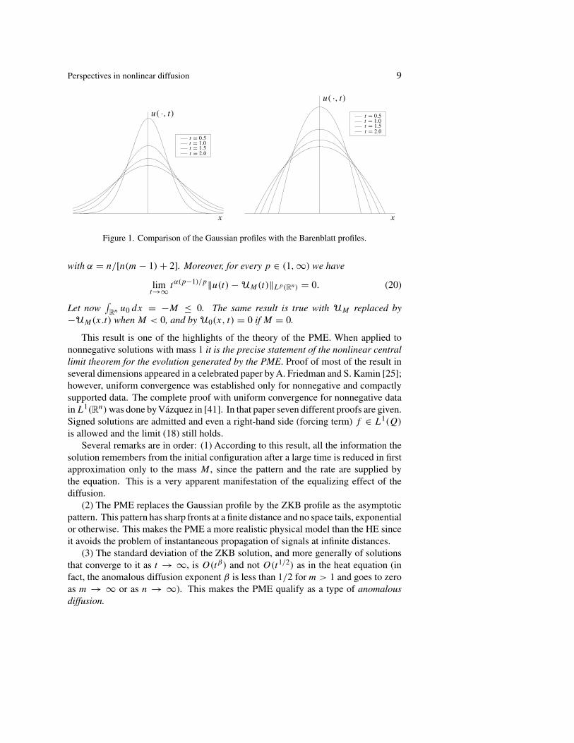
The constant C > 0 is free and can be used to adjust the mass of the solution:∫Rn U(x, t; C) dx = M > 0. Let us write UM for the solution with mass M and FM

for its profile. Figure 1 compares the profiles.This is the precise statement of the asymptotic convergence result.

Theorem 4.1. Let u(x, t) be the unique weak solution of the Cauchy problem for thePME posed in Q = R

n × (0, ∞) with initial data u0 ∈ L1(RN), and∫

Rn u0 dx =M > 0. Let UM be the ZKB solution with the same mass as u0. As t → ∞ thesolutions u(t) and UM are increasingly close and we have

limt→∞ ‖u(t) − UM(t)‖1 = 0. (18)

Convergence holds also in L∞-norm in the proper scale:

limt→∞ tα‖u(t) − UM(t)‖∞ = 0 (19)


u( ·, t)

x

t = 0.5t = 1.0t = 1.5t = 2.0

u( ·, t)

x

t = 0.5t = 1.0t = 1.5t = 2.0

Figure 1. Comparison of the Gaussian profiles with the Barenblatt profiles.

with α = n/[n(m − 1) + 2]. Moreover, for every p ∈ (1, ∞) we have

limt→∞ tα(p−1)/p‖u(t) − UM(t)‖Lp(Rn) = 0. (20)

Let now∫

Rn u0 dx = −M ≤ 0. The same result is true with UM replaced by−UM(x.t) when M < 0, and by U0(x, t) = 0 if M = 0.

This result is one of the highlights of the theory of the PME. When applied tononnegative solutions with mass 1 it is the precise statement of the nonlinear centrallimit theorem for the evolution generated by the PME. Proof of most of the result inseveral dimensions appeared in a celebrated paper by A. Friedman and S. Kamin [25];however, uniform convergence was established only for nonnegative and compactlysupported data. The complete proof with uniform convergence for nonnegative datain L1(Rn) was done by Vázquez in [41]. In that paper seven different proofs are given.Signed solutions are admitted and even a right-hand side (forcing term) f ∈ L1(Q)

is allowed and the limit (18) still holds.Several remarks are in order: (1) According to this result, all the information the

solution remembers from the initial configuration after a large time is reduced in firstapproximation only to the mass M , since the pattern and the rate are supplied bythe equation. This is a very apparent manifestation of the equalizing effect of thediffusion.

(2) The PME replaces the Gaussian profile by the ZKB profile as the asymptoticpattern. This pattern has sharp fronts at a finite distance and no space tails, exponentialor otherwise. This makes the PME a more realistic physical model than the HE sinceit avoids the problem of instantaneous propagation of signals at infinite distances.

(3) The standard deviation of the ZKB solution, and more generally of solutionsthat converge to it as t → ∞, is O(tβ) and not O(t1/2) as in the heat equation (infact, the anomalous diffusion exponent β is less than 1/2 for m > 1 and goes to zeroas m → ∞ or as n → ∞). This makes the PME qualify as a type of anomalousdiffusion.


(4) The convergence also takes place for the rescaled version of the equation inthe Wasserstein distance d2 [37]. But this is a different story in some sense.

(5) For a given solution u, there is only one correct choice of the constant C =C(u0) in these asymptotic estimates, since trying two ZKB solutions with differentconstants in the above formulas produces non-zero limits. In that sense, the estimatesare sharp.

(6) The result is optimal in the sense that we cannot get better convergence ratesin the general class of solutions u0 ∈ L1(Rn), even if we assume u0 ≥ 0. Explicitcounterexamples settle this question.

(7) It can be further proved that whenever m > 1 and we take signed initialdata with compact support and the total mass is positive, M > 0, then, the solutionbecomes nonnegative after a finite time. This result is not true if the restriction ofcompact support is eliminated.

Proof by scaling. The idea is as follows: given a solution u = u(x, t) ≥ 0 of thePME in the class of strong solutions with finite mass, we obtain a family of solutions

uλ(x, t) = (Tλu)(x, t) = λαu(λβx, λ t) (21)

with initial data u0,λ(x) = (Tλu0)(x) = λαu0(λβx). The exponents α and β are

related byα(m − 1) + 2β = 1, (22)

so that all the uλ are again solutions of the PME. This is the scaling formula that wecall the λ-scaling or fixed scaling. It is in fact a family of scalings with free parameterλ > 0, that performs a kind of zoom on the solution. In the present application wehave another constraint that allows to fix both α and β to the desired values (theBarenblatt values). It is the condition of mass conservation. We only need to imposeit at t = 0, ∫

Rn

(Tλu0)(x) dx =∫

Rn

u0(x) dx, (23)

and we get α = n β. Together with (22), this implies that α and β have the values(17) of the theorem. Note that the source-type solutions are invariant under this massconserving λ-rescaling, i.e.

UM(t) = Tλ(UM(t)).

The proof continues by showing that the family {uλ(t), λ > 0}, is uniformly boundedand even relatively compact in suitable functional spaces. We then pass to the limitdynamics when λ → ∞ and identify the obtained object as the ZKB solution. Werefer to [44]; Chapter 18, for complete details on the issue.

4.1. Continuous scaling: Fokker–Planck equation. A different way of implemen-ting the scaling of the orbits of the Cauchy problem and proving the previous factsconsists of using the continuous rescaling, which is written in the form

θ(η, τ ) = tαu(x, t), η = x t−β, τ = ln t, (24)


with α and β the standard similarity exponents given by (17). Then tα and tβ arecalled the scaling factors (or zoom factors), while τ is the new time. This versionof the scaling technique has a very appealing dynamical flavor. The reader shouldnote that every asymptotic problem has its corresponding zoom factors that have tobe determined as a part of the analysis. In our case, the rescaled orbit θ(τ ) satisfiesthe equation

θτ = �(θm) + βη · ∇θ + αθ. (25)

This is the continuously rescaled dynamics. Since we also have the relation α = n β,we can write the equation in divergence form as

θτ = �(θm) + β ∇ · (η θ). (26)

This is a particular case of the so-called Fokker–Planck equations which have thegeneral form

∂tu = �(|u|m−1u) + ∇ · (a(x)u), a(x) = ∇V (x). (27)

The last term is interpreted as a confining effect due to a potential V . In our caseV (x) = β |x|2/2, the quadratic potential. The study of Fokker–Planck equations isinteresting in itself and not only in connection with the HE and the PME.

This dynamical systems approach allows us to see the contents of the asymptotictheorem in a better way: the orbit θ(τ ) is bounded uniformly in L1(Rn) ∩ L∞(Rn);the source-type (ZKB) solutions transform into the stationary profiles FM in thistransformation, i.e., F(η) solves the nonlinear elliptic problem

�f m + β ∇ · (η f ) = 0; (28)

moreover, boundedness of the orbit is established; this and convenient compactnessarguments allow to pass to the limit and form the ω-limit, which is the set

ω(θ) = {f ∈ L1(�) : there exists {τj } → ∞ such that θ(τj ) → f }. (29)

The convergence takes place in the topology of the functional space in question, hereany Lp(�), 1 ≤ p ≤ ∞. The end of the proof consists in showing that the ω-limitis just the Barenblatt profile FM . The argument can be translated in the followingway. Corresponding to the sequence of scaling factors λn of the previous scaling, wetake a sequence of delays {sn} and define θn(η, τ ) = θ(η, τ + sn). The family {θn} isprecompact in L∞

loc(R+ : L1(Rn)) hence, passing to a subsequence if necessary, wehave

θn(η, τ ) → θ (η, τ ). (30)

Again, it is easy to see that θ is a weak solution of (26) satisfying the same estimates.The end of the proof is identifying it as a stationary solution, θ (η, τ ) = FM(η), theBarenblatt profile of the same mass.


4.2. The entropy approach: convergence rates. A number of interesting resultscomplement this basic convergence result in the recent literature. Thus, the questionof obtaining an estimate of the rate at which rescaled trajectories of the PME sta-bilize towards the Barenblatt profile has attracted much attention. The main tool ofinvestigation has been the consideration of the so-called entropy functional, definedas follows

Hθ(τ) =∫

Rn

{1

m − 1θm + β

2η2 θ

}dη, (31)

where θ = θ(η, τ ) is the rescaled solution just defined and β = 1/(n(m−1)+2) is thesimilarity exponent. Hθ represents a measure of the entropy of the mass distributionθ(τ ) at any time τ ≥ 0 which is well adapted to the renormalized PME evolution.Note that the entropy need not be finite for all solutions, a sufficient condition is

u0 ∈ L1(Rn) ∩ L∞(Rn),

∫x2u0(x) dx < ∞. (32)

These properties will then hold for all times. Note that the restriction of boundednessis automatically satisfied for positive times.

Actually, we can calculate the variation of the entropy in time along an orbit ofthe Fokker–Planck equation, and under the above conditions on u0, we find after aneasy computation that

dHθ

dτ= −Iθ , where Iθ (τ ) =

∫θ

∣∣∣∣∇ (m

m − 1θm−1 + β

2η2

)∣∣∣∣2

dη ≥ 0. (33)

We now pass to the limit along sequences θn(τ ) = θ(τ + sn) to obtain limit orbitsθ (τ ), on which the Lyapunov function is constant, hence dHθ/dτ = 0. The proof ofasymptotic convergence concludes in the present instance in a new way, by analyzingwhen dHθ/dτ is zero. Here is the crucial observation that ends the proof: the secondmember of (33) vanishes if and only if θ is a Barenblatt profile.

Let us now introduce some notations: the difference H(θ |θ∞) = H(θ)−H(θ∞)

is called the relative entropy. Function Iθ is called the entropy production. We canuse the entropy functional to improve the convergence result by obtaining rates ofconvergence. This is done by computing d2Hθ/dτ 2, the so-called Bakry–Emeryanalysis in the heat equation case which has been adapted to the PME by J. A. Carrilloand G. Toscani [17]. The final result of the second derivative computation is

dI

dτ= −2β I (τ) − R(τ), (34)

for a certain term R ≥ 0. Since we know by the previous analysis that H(θ |θ∞) andIθ go to zero as τ → ∞, we conclude the following result.

Theorem 4.2. Under the assumption that the initial entropy is finite and some regu-larity assumptions, we have

I (τ ) ≤ A e−2βτ , 0 ≤ H(θ |θ∞)(τ ) ≤ 1

2βI (τ), H(θ |θ∞) ≤ B e−2βτ . (35)


As a consequence, the convergence towards the ZKB stated in Theorem 4.1 happenswith an extra factor tγ in formulas (18)–(20), where

γ = β if 1 < m ≤ 2, γ = 2β

mif m ≥ 2, (36)

and β = 1/(n(m − 1) + 2).

In dimension n = 1, a convergence theorem with sharp rates can be proved byadjusting not only the mass but also the center of mass, cf. [40]. It is an open problemfor n > 1.

4.3. Eventual concavity. There are many other directions in which the asymptoticbehaviour of the PME is made more precise. This is the geometrical result obtainedby Lee–Vázquez [34] (Figure 2 shows a practical instance).

Theorem 4.3. Let u be a solution of the PME in n ≥ 1 space dimensions withcompactly supported initial data (and satisfying a certain non-degeneracy condition).Then there is tc > 0 such that the pressure v(x, t) is a concave function in P (t) ={x : v(x, t) > 0} for t ≥ tc. More precisely, for any coordinate directions xi , xj ,

limt→∞ t

∂2v

∂x2i

= −β, limt→∞ t

∂2v

∂xi∂xj

= 0, (37)

uniformly in x ∈ supp(v), i, j = 1, . . . , n, i �= j . Here, β = 1/(n(m − 1) + 2).

−15 −10 −5 0 5 10 15−1

0

1

2

3

4

5

6

7

Figure 2. Evolution towards selfsimilarity and eventual concavity in the PME.

4.4. Extensions. In the case of the Cauchy–Dirichlet problem posed in a boundeddomain � ⊂ R

N , it is well known that the asymptotic shape of any solution of theheat equation with nonnegative initial data in L2(�) approaches one of the specialseparated variables solutions

u1(x, t) = c T1(t) F1(x). (38)


Here T1(t) = e−λ1t , where λ1 = λ1(�) > 0 is the first eigenvalue of the Laplaceoperator in � with zero Dirichlet data on ∂�, and the space pattern F1(x) is the cor-responding positive and normalized eigenfunction. The constant c > 0 is determinedas the coefficient of the L2(�)-projection of u0 on F1. For the PME a similar resultis true with the following differences: F1(x) is the ground state of a certain nonlineareigenvalue problem, while T1(t) = t−1/(m−1), which means power decay in time.For signed solutions there exists a whole sequence of compactly supported profilesFk(x) as candidates for the separation-of-variables formula (38), but the time factoris always the same T1(t) = t−1/(m−1); this is a striking difference with the linear casein which the exponentials have an increasing sequence of coefficients.

The analysis applies to the homogeneous Neumann problem and leads to a markeddifference between data with positive or negative mass, where the solutions stabilizeto the constant state with exponential speed (just as linear flows) and the case of zeromass, where the t−1/(m−1) time factor appears.

Another extension consists of considering the whole space with a number of holes;Dirichlet or Neumann boundary conditions are imposed on the boundary � of theholes. If for instance conditions of the form u = 0 are chosen on �, then theBarenblatt profiles still appear as the asymptotic patterns in dimension n ≥ 3, butnot in dimension n = 1 while dimension n = 2 is a borderline case [30], [9].Actually, the influence of the holes is felt in terms of their capacity, which has aninteresting physico-geometrical interpretation. Dependence on dimension is verytypical of nonlinear diffusion problems, it will appear again in fast diffusion flowsand is a very prominent feature in blow-up problems.

5. Some lines of research

The theory of the PME is by now well understood in the case of dimension one, but itstill has gaps for n > 1 because n dimensional PME flows turned out to be much morecomplicated. Thus, the regularity of nonnegative solutions is effectively solved forn = 1 by stating the best Hölder regularity (the pressure is Lipschitz continuous but notC1) and showing the worst case situation, that corresponds to the presence of movingfree boundaries that always follow the same pattern, the solution locally behaveslike a travelling wave. The same question in dimension n > 1 is still only partiallyunderstood even after intensive work of D. Aronson and coworkers [2], [3] on the so-called focusing problem. They discovered first the radial solutions with limited Hölderregularity and then the nonradial focusing modes with elongated shapes bifurcatingfrom the radial branch as m varies (a typical break of stability in a bifurcation branch,somewhat similar to the Taylor–Couette hydrodynamical instabilities).

After the work of L. Caffarelli et al. [12], [15], the C∞ regularity of the solutionsup to the free boundary and also of the free boundary as a hypersurface was provedfor large times by H. Koch [32] under convenient conditions on the data, but furtherprogress is expected.


Even in the theory of nonnegative solutions of the Cauchy problem for the PME,there are still some basic analytical problems, like the following: the theory isvery much simplified by the existence of the Aronson–Bénilan pointwise estimate�um−1 ≥ −C/t . A local version of this estimate is known only in dimension n = 1.

On the other hand, the question of obtaining solutions for the widest possibleclass of initial data has been successfully solved for nonnegative solutions, but onlypartially understood for signed solutions. See [44], Chapters 12 and 13.

If we replace the exponent 2 by p ∈ [1, ∞] in the Wasserstein formula (13), weget the Wasserstein non-quadratic distances. The PME semigroup is contractive inall of them in dimension n = 1. In particular, contraction in the d∞ norm allows forfine estimates of the support propagation. Unfortunately, the PME semigroup is notcontractive in the distance dp for p large if n > 1, [42]. Actually, a similar negativeresult happens for the usual Lp norms in all space dimensions, see [44]. Determiningthe precise ranges of p for these contractivity issues is still an open problem.

6. Fast diffusion equations: physics and geometry

The fast diffusion equation is formally the same as the PME but the exponent is nowm < 1. It appears in several areas of mathematics and science when the assumptionsof linear diffusion are violated in a direction contrary to the PME. Here are someexamples.

• Plasma diffusion with the Okuda–Dawson scaling implies a diffusion coefficientD(u) ∼ u−1/2 in the basic equation ut = ∇ · (D(u)∇u), where u is the particledensity. This leads to the FDE with m = 1/2. Other models imply exponents m = 0,D(u) ∼ 1/u, or even m = −1, D(u) ∼ 1/u2.

• A very popular fast diffusion model was proposed by Carleman to study the diffusivelimit of kinetic equations. He considered just two types of particles in a one dimen-sional setting moving with speeds c and −c. If the densities are u and v respectivelyyou can write their simple dynamics as

∂tu + c ∂xu = k(u, v)(v − u)

∂tv − c ∂xv = k(u, v)(u − v)

}(39)

for some interaction kernel k(u, v) ≥ 0. Put in a typical case k = (u + v)αc2. Writenow the equations for ρ = u+v and j = c(u−v) and pass to the limit c = 1/ε → ∞and you will obtain to first order in powers or ε = 1/c:

∂ρ

∂t= 1

2

∂

∂x

(1

ρα

∂ρ

∂x

), (40)

which is the FDE with m = 1 − α, cf. [35]. The typical value α = 1 gives m = 0, asurprising equation that we will find below! The rigorous investigation of the diffusionlimit of more complicated particle/kinetic models is an active area of investigation.


• The fast diffusion makes a striking appearance in differential geometry, in the evo-lution version of the Yamabe problem. The standard Yamabe problem starts with aRiemannian manifold (M, g0) in space dimension n ≥ 3 and deals with the questionof finding another metric g in the conformal class of g0 having constant scalar cur-vature. The formulation of the problem proceeds as follows in dimension n ≥ 3. Wecan write the conformal relation as

g = u4/(n−2)g0

locally on M for some positive smooth function u. The conformal factor is u4/(n−2).Next, we denote byR = Rg andR0 the scalar curvatures of the metricsg, g0 resp. If wewrite �0 for the Laplace–Beltrami operator of g0, we have the formula R = −u−NLu

on M, with N = (n + 2)/(n − 2) and

Lu := κ�0u − R0u, κ = 4(n − 1)

n − 2.

The Yamabe problem becomes then

�0u −(

n − 2

4(n − 1)

)R0u +

(n − 2

4(n − 1)

)Rgu

(n+2)/(n−2) = 0. (41)

The equation should determine u (hence, g) when g0, R0 and Rg are known. In thestandard case we take M = R

n and g0 the standard metric, so that �0 is the standardLaplacian, R0 = 0, we take Rg = 1 and then we get the well-known semilinearelliptic equation with critical exponent.

In the evolution version, theYamabe flow is defined as an evolution equation for afamily of metrics that is used as a tool to construct metrics of constant scalar curvaturewithin a given conformal class. More precisely, we look for a one-parameter familygt (x) = g(x, t) of metrics solution of the evolution problem

∂tg = −R g, g(0) = g0 on M. (42)

It is easy to show that this is equivalent to the equation

∂t (uN) = Lu, u(0) = 1 on M.

after rescaling the time variable. Let now (M, g0) be Rn with the standard flat metric,

so that R0 = 0. Put uN = v, m = 1/N = (n − 2)/(n + 2) ∈ (0, 1). Then

∂tv = Lvm, (43)

which is a fast diffusion equation with exponent my ∈ (0, 1) given by

my = n − 2

n + 2, 1 − my = 4

n + 2.


If we now try separate variables solutions of the form v(x, t) = (T − t)αf (x), thennecessarily α = 1/(1−my) = (n+2)/4, and F = f m satisfies the semilinear ellipticequation with critical exponent that models the stationary version:

�F + n + 2

4F

n+2n−2 = 0. (44)

We will stop at this point the motivation of nonlinear diffusion coming from geom-etry, to return later with the logarithmic diffusion. The influence of PDE techniquesis strongly felt in present-day differential geometry, cf. A. Chang’s exposition at the2002 ICM [18].

6.1. Behaviour of fast diffusion flows: the good range. For values m ∼ 1 thedifference with the PME is noticed in the infinite speed of propagation: solutionswith nonnegative data become immediately positive everywhere in the space domain(be it finite or infinite). This looks like the heat equation and in some sense it is. Whenwe look at the source solutions we find explicit Barenblatt functions

Um(x, t; M)1−m = t

C t2α/n + k1 x2 , (45)

with C = a(m, n)M2(m−1)α/n and k1 is an explicit function of m and n. Figure 3shows the form.

u( ·, t)

x

t = 1.15t = 1.25t = 1.40t = 1.60

Figure 3. The fast diffusion solution with fat tails.

The main difference in the ZKB profiles is the power-like tail at infinity, which verymuch differs from the Gaussian (exponential) behaviour. These tails, called fat tails,are currently the object of study in several areas of economy, finance and statisticalphysics and their properties and role are still not well understood.

The new Barenblatt solutions play the same role they played for m > 1 even ifthey have a different shape. Indeed, the asymptotic behaviour of general solution is


still described by Theorem 4.1 if mc < m < 1, where mc = (n − 2)+/n is called thefirst critical exponent. Actually, the convergence is better: we have proved in [41]that the relative error e(x, t) = u(x, t)/Um(x, t) − 1 converges to zero uniformlyin x as t → ∞, a property that is obviously false for m > 1 because of the (slightly)different supports.

6.2. Behaviour of fast diffusion flows: the subcritical range. Significant novel-ties in the mathematical theory of the FDE appear once we cross the line m = mc

downwards. Then, the picture changes and we enter a realm of strange diffusions.Note that mc is larger than the Yamabe exponent my . Thus, concerning the basicproblem of optimal space for existence, H. Brezis and A. Friedman proved in [10]that there can be no solution of the equation if m ≤ mc when the initial data is a Diracmass, so that we lose the source solution, our main example of the range m > mc.M. Pierre [39] extended the non-existence result to measures supported in sets of smallcapacity if m < mc. But at least solutions exist for all initial data u0 ∈ L1

loc(Rn) when

0 < m < mc, and moreover they are global in time, u ∈ C([0, ∞) : L1loc(R

n)). Suchan existence result is not guaranteed when we go further down in exponent, m ≤ 0;then, solutions with initial data in L1(Rn) just do not exist.

However, and contrary to the ‘upper’ fast diffusion range mc < m < 1, it is nottrue that locally integrable data produce locally bounded solutions at positive times,as in the various examples constructed in [43]. Attention must be paid therefore tothe existence and properties of large classes of weak solutions that are not smooth,not even locally bounded. This leads to a main fact to be pointed out about smoothingestimates: there can be no L1-L∞ effects.

Extinction and Marcinkiewicz spaces. For m < mc (even for m ≤ 0) there is anexplicit example of solution which completely vanishes in finite time, and has theform

U(x, t; T ) = c

(T − t

|x|2)1/(1−m)

(46)

with T > 0 arbitrary, and c = c(m, n) > 0 a given constant. Formula (46) pro-duces a weak solution of the FDE that is positive and smooth for 0 < t < T

and x �= 0; note further that it belongs to the Marcinkiewicz space Mp∗(Rn) withp∗ = n(1 − m)/2, a quantity that is larger than 1 if m < mc.

The positive result that we can derive from comparison with this solution is thefollowing.

Theorem 6.1. Let n ≥ 3 and m < mc. For every u0 ∈ Mp∗(Rn), there exists a timeT > 0 such that u(x, t) vanishes for t ≥ T . It can be estimated as

0 < T ≤ d ‖u0‖1−mMp∗ := T1(u0) (47)

with d = d(m, n) > 0. Moreover, for all 0 < t < T we have u(t) ∈ Mp∗(Rn) andu∗(t) ≺ U(t; T ) where T is chosen so that U(x, 0; T ) has the same Mp∗-norm asu0, i.e., M = cmT 1−m.


The relevant functional spaces Mp(Rn) are the so-called Marcinkiewicz spacesor weak Lp spaces, defined for 1 < p < ∞ as the set of locally integrable functionssuch that ∫

K

|f (x)|dx ≤ C|K|(p−1)/p,

for all subsets K of finite measure. It is further proved that solutions with data inthe space Mp(Rn) with p > p∗ become bounded for all positive times and do notnecessarily extinguish in finite time, while solutions with data in the space Mp(Rn)

with 1 < p < p∗ become L1 functions for all positive times and do not necessarilyextinguish in finite time, see [43], Chapter 5. While becoming bounded is a typicalfeature of the parabolic theory (called the L∞ smoothing effect), becoming L1 is akind of extravaganza that happens for these fast diffusion flows (it was introduced andcalled backward effect in [43]).

Delayed regularity. A further curious effect is proved in Chapter 6 of the samereference: functions in the larger space Mp∗(Rn) + L∞(Rn) typically preserve theirunboundedness for a time T > 0 and then become bounded. This is also calledblow-down in finite time.

Large-time behaviours: selfsimilarity with anomalous exponents. The actualasymptotic behaviour of the solutions of the FDE in the exponent range 0 < m <

mc depends on the class of initial data. We are interested in “small solutions” thatextinguish in finite time, We will concentrate on solutions that start with initial data inL1(Rn), or solutions that fall into this class for positive times previous to extinctionby the backward effect. In the range m > mc the ZKB solutions provide the clueto the asymptotics for all nonnegative solutions with L1-data. We know that thesesolutions do not exist in the range m < mc. So we need to look for an alternative. Thisalternative has to take into account the fact that solutions with Mp∗-data disappear(vanish identically) in finite time.

The class of self-similarity solutions of the form

U(x, t) = (T − t)αf (x (T − t)β), (48)

called selfsimilar of Type II, will provide the clue to the asymptotic behaviour nearextinction. We have to find the precise exponents and profile that correspond to a so-lution of the form (48) and represent the large time behaviour of many other solutions.We know from the start that α(1−m) = 2β +1. But there is no conservation law thatdictates to us the remaining relation needed to uniquely identify the exponents. Thismay seem hopeless but the representative solutions exist and have precise exponentsand profile. This is a situation that appears with a certain frequency in mechanics andwas called by Y. Zel’dovich self-similarity of the second kind, the exponents beingknown as anomalous exponents. Anomalous means here that the exponents cannotbe obtained from dimensional considerations or conservation laws, as is done in theZKB case by means of the scaling group. Such kind of solutions is of great interestbecause of their analytical difficulty.


The selection rule for the anomalous exponents is usually topological, tied to theexistence and behaviour of the solutions of a certain nonlinear eigenvalue problem.In the present case, the selection is done through the existence of a special class ofself-similar solutions with fast decay at infinity. The construction was performed byJ. King, M. Peletier and H. Zhang [31], [38] and is extended and described in detailin [43], Chapter 7. We call them KPZ solutions.

We can then pass to the question of convergence of general classes of solutionstowards the KPZ solutions. This is in analogy to the results for the ZKB profiles form > mc. The results are more complete when m = my , where the problem has anice geometrical interpretation. The proof of convergence results towards the KPZsolution is only known in the case of radial solutions when m �= my , cf. [26].

FDE with exponent m = (n − 2)/(n + 2): Yamabe problem. The exponent isspecial in the sense that when we separate variables and pass to the Emden–Fowlerequation for G = Fm

−�G = Gp, (49)

then p = 1/m equals the Sobolev exponent ps = (n + 2)/(n − 2), that is knownto have a great importance in the theory of semilinear elliptic equations. We maythus call my the Sobolev exponent of the FDE. We recall that the FDE is related forthis precise exponent to the famous Yamabe flow of Riemannian geometry. As wehave said, this flow is used by geometers as a tool to deform Riemannian metrics intometrics of constant scalar curvature within a given conformal class. Returning to theconsideration of the family of KPZ solutions with anomalous exponents, this is the“easy case” whereβ = 0 (that corresponds to separate variables) so thatα = (n+2)/4.The corresponding family of self-similar solutions is explicitly known and given bythe Loewner–Nirenberg formula

F(x, λ) = kn

(λ

λ2 + |x|2)(n+2)/2

(50)

with kn = (4n)(n+2)/4 and λ > 0 arbitrary. These patterns represent conformalmetrics with constant curvature in the geometrical interpretation. Here is the resultof [21] as improved in [43], Chapter 7.

Theorem 6.2. Let n ≥ 3 and m = (n − 2)/(n + 2) and let u(x, t) ≥ 0 be asolution of the FDE existing for a time 0 < t < T . Under the assumption thatu0 ∈ L2n/(n+2)(Rn) the solution of the FDE is bounded for all t > 0. Moreover, thereexist λ and x0 ∈ R

n such that

(T − t)−(n+2)/4u(x, t) = F(x − x0, λ) + θ(x, t) (51)

and ‖θ(t)‖Lp∗ → 0 as t → T . The exponent in the space assumption is optimal.

We just recall that p∗ = 2n/(n + 2) in the present case.


Exponential decay at the critical end-point. Inspection of the ZKB solutions as m

goes down to mc shows that asymptotic decay happens as t → ∞ with increasingpowers of time, i.e., u ∼ t−α and α → ∞. Exponential decay holds for the FDE withcritical exponent mc for a large number of initial, but not for all L1 data. We have

Theorem 6.3. Let m = mc and n ≥ 3. Solutions in L1(Rn) ∩ L∞(Rn) decay in timeaccording to the rate

log(1/‖u(t)‖∞) ∼ C(n)M−2/(n−2)tn/(n−2) (52)

as t → ∞, M = ‖u0‖1. This rate is sharp.

This behaviour is not selfsimilar and has been calculated by V. Galaktionov,L. Peletier and J. L. Vázquez in [27], based on previous formal analysis of J. King[31]. The proof uses a delicate technique of matched asymptotics with an outer regionwhich after a nonlinear transformation undergoes convergence to a selfsimilar profileof convective type. This is said here to show that unexpected patterns can appear asthe result of these manipulations. Slower pace of decay happens for non-integrablesolutions, as the following selfsimilar example shows

u(x, t) = 1

(bx2 + ke2nbt )n/2 , b, k > 0. (53)

7. Logarithmic diffusion

The fast diffusion equation in the limit case m = 0 in two space dimensions is afavorite case in the recent literature on fast diffusion equations. The equation can bewritten as

∂tu = div (u−1∇u) = � log(u), (54)

hence the popular name of logarithmic diffusion. The problem has a particular appealbecause of its application to differential geometry, since it describes the evolution ofsurfaces by Ricci flow. More precisely, it represents the evolution of a conformallyflat metric g by its Ricci curvature,

∂

∂tgij = −2 Ricij = −R gij , (55)

where Ric is the Ricci tensor and R the scalar curvature. If g is given by the lengthexpression ds2 = u (dx2 + dy2), we arrive at equation (54). This flow, proposedby R. Hamilton in [29], is the equivalent of the Yamabe flow in two dimensions. Weremark that what we usually call the mass of the solution (thinking in diffusion terms)becomes here the total area of the surface, A = ∫∫

u dx1dx2.Several peculiar aspects of the theory are of interest: non-uniqueness, loss of mass,

regularity and asymptotics. Maybe the most striking is the discovery that conservationof mass is broken in a very precise way.

• Let us consider integrable data. This is the basic result of the theory.


Theorem 7.1. For every u0 ∈ L1(R2), with u0 ≥ 0 there exists a unique functionu ∈ C([0, T ) : L1(R2)), which is a classical (C∞ and positive) solution of (54) inQT and satisfies the area constraint∫

u(x, t)dx =∫

u0(x)dx − 4π t. (56)

Such solution is maximal among the solutions of the Cauchy problem for (54) withthese initial data, and exists for the time 0 < t < T = ∫

R2 u0(x) dx/4π . Moreover,the solution is obtained as the limit of positive solutions with initial data u0ε(x) =u0(x) + ε as ε → 0.

The mysterious loss of 4π units of area (mass) has attracted the attention ofresearchers. In the geometrical application it is quite easy to see it as a form ofthe Gauss–Bonnet theorem. It is shown that the Gaussian curvature K is given byK = �u/2u, and then∫

R2ut dx = −2

∫M

K d Volg = −4π.

There are also analytical proofs of this fact, that look a bit mysterious, see [43],Chapter 8.

• One of the peculiar properties of this equation is the existence of multiple solutionswith finite area with the same initial data that are characterized by the behaviour atinfinity. The situation is completely understood in the radial case and the followinggeneral result is proved.

Theorem 7.2. For every nonnegative radial function u0 ∈ L1(R2) and for everybounded function f (t) ≥ 2, there exists a unique function u ∈ C([0, T ) : L1(R2)),which is a radially symmetric and classical solution of (P0) in QT and satisfies themass constraint ∫

u(x, t)dx =∫

u0(x)dx − 2π

∫ t

0f (τ) dτ. (57)

It exists as long as the integral in the LHS is positive. The case f = 0 correspondsto the maximal solution of the Cauchy problem. In any case, the solution is boundedfor all t > 0.

Thus, not only there are infinitely many solutions for every fixed nontrivial initialfunction u0, but also the extinction time can be controlled by means of the flux data f .Moreover, these solutions satisfy the asymptotic spatial behaviour

limr→∞ r ∂r(log u(r, t)) = −f (t) (58)

for a.e. t ∈ (0, T ). Non-uniqueness extends to non-integrable solutions. Thus, thestationary profile

u(x1, x2, t) = AeBx1, A, B > 0,


is not the unique solution with such data, it is not even the maximal solution.

• Actually, the geometrical interpretation in the case of data with finite area favors theflow with conditions at infinity f = 4, hence the mass loss per unit time equals 8π ,which are interpreted as regular closed compact surfaces. Here is the most typicalexample

u(x, t) = 8(T − t)

(1 + x2)2 , (59)

which represents the evolution of a ball with total area∫

u(x, t) dx = 8π(T − t).

• Coming to the regularity question, solutions with data in L1(R2) are bounded. Butthe limit when the data tend to a measure, more precisely to a Dirac mass, is notincluded. Indeed, when we approximate a Dirac delta Mδ(x) by smooth integrablefunctions ϕn(x), solve the problem in the sense of maximal solutions un(x, t) andpass to the limit in the approximation, the following result is obtained

limn→∞ un(x, t) = (M − 4πt)+δ(x). (60)

In physical terms, it means that logarithmic diffusion is unable to spread a Dirac mass,but somehow it is able to dissipate it in finite time. A delicate thin layer process occursby which the mass located at x = 0 is transferred to x = ∞ without us noticing.We explain this phenomenon in the recent paper [45] where the following result isproved: we assume that the initial mass distribution can be written as

dμ0(x) = f (x)dx +k∑

i=1

Mi δ(x − xi). (61)

where f ≥ 0 is an integrable function in R2, the xi , i = 1, . . . , k, are a finite collection

of (different) points on the plane, and we are given masses 0 < Mk ≤ · · · ≤ M2 ≤ M1.The total mass of this distribution is

M = M0 +k∑

i=1

Mi, with M0 =∫

f dx. (62)

We construct a solution for this problem as the limit of natural approximate prob-lems with smooth data:

Theorem 7.3. Under the stated conditions, there exists a limit solution of the log-diffusion Cauchy problem posed in the whole plane with initial data μ0. It exists inthe time interval 0 < t < T with T = M/2π . It satisfies the conditions of maximalityat infinity.

More precisely, the solution is continuous into the space of Radon measures,u ∈ C([0, T ] : M(R2)), and it has two components, singular and regular. The


singular part amounts to a collection of (shrinking in time) point masses concentratedon the points x = xi of the precise form

using =∑

i

(Mi − 4πt)+δ(x − xi). (63)

The regular part can be described as follows:(i) When restricted to the perforated domain Q∗ = (

R2 − ⋃

i{xi}) × (0, T ), u is

a smooth solution of the equation, it takes the initial data f (x) for a.e. x �= xi , andvanishes at t = T .

(ii) At every time t ∈ (0, T ) the total mass of the regular part is the result of addingto M0 the inflow coming from the point masses and subtracting the outflow at infinity.

(iii) Before each point mass disappears, we get a singular behaviour near the masslocation as in the radial case, while later on the solution is regular around that point.

For complete details on this issue we refer to [45].The theory of measure-valued solutions of diffusion equations is still in its begin-

ning. A large number of open problems are posed for subcritical fast diffusion.

References

[1] Andreu-Vaillo, F., Caselles, V., Mazón, J. M., Parabolic quasilinear equations minimizinglinear growth functionals. Progr. Math. 223, Birkhäuser, Basel 2004.

[2] Angenent, S. B., Aronson, D. G., Betelu, S. I., Lowengrub, J. S., Focusing of an elongatedhole in porous medium flow. Phys. D 151 (2–4) (2001), 228–252.

[3] Aronson, D. G., Graveleau, J. A., Self-similar solution to the focusing problem for theporous medium equation. European J. Appl. Math. 4 (1) (1993), 65–81.

[4] Barenblatt, G. I., Scaling, Self-Similarity, and Intermediate Asymptotics. Cambridge Uni-versity Press, Cambridge 1996; updated version of Similarity, Self-Similarity, and Inter-mediate Asymptotics, Consultants Bureau, New York 1979.

[5] Barenblatt, G. I., Scaling. Cambridge Texts in Appl. Math., Cambridge University Press,Cambridge, 2003.

[6] Bénilan, P., Equations d’évolution dans un espace de Banach quelconque et applications.Ph. D. Thesis, Université Orsay, 1972 (in French).

[7] Bénilan, P., Carrillo, J., Wittbold, P., Renormalized entropy solutions of scalar conservationlaws. Ann. Scuola Norm. Sup. Pisa Cl. Sci. (4) 29 (2) (2000), 313–327.

[8] Brändle, C., Vázquez, J. L., Viscosity solutions for quasilinear degenerate parabolic equa-tions of porous medium type. Indiana Univ. Math. J. 54 (3) (2005), 817–860.

[9] Brändle, C., Quirós, F., Vázquez, J. L., Asymptotic behaviour of the porous media equationin domains with holes. Interfaces Free Bound., to appear.

[10] Brezis, H., Friedman, A., Nonlinear parabolic equations involving measures as initial con-ditions. J. Math. Pures Appl. 62 (1983), 73–97.

[11] Caffarelli, L. A., Cabré, X., Fully nonlinear elliptic equations. Amer. Math. Soc. Colloq.Publ. 43, Amer. Math. Soc., Providence, RI, 1995.


[12] Caffarelli, L. A., Friedman, A., Regularity of the free boundary of a gas flow in an n-dimen-sional porous medium. Indiana Univ. Math. J. 29 (1980), 361–391.

[13] Caffarelli, L. A., Salsa, S., A geometric approach to free boundary problems. Grad. Stud.Math. 68, Amer. Math. Soc., Providence, R.I., 2005.

[14] Caffarelli, L.A.,Vázquez, J. L.,Viscosity solutions for the porous medium equation. In Dif-ferential equations: La Pietra 1996 (ed. by M. Giaquinta, J. Shatah and S. R. S. Varadhan),Proc. Sympos. Pure Math. 65, Amer. Math. Soc., Providence, RI, 1999, 13–26.

[15] Caffarelli, L. A., Vázquez, J. L., Wolanski, N. I., Lipschitz continuity of solutions andinterfaces of the N-dimensional porous medium equation. Indiana Univ. Math. J. 36 (1987),373–401.

[16] Carrillo, J. A., McCann, R., Villani, C., Contractions in the 2-Wasserstein length space andthermalization of granular media. Arch. Rational Mech. Anal. 179 (2006), 217–264.

[17] Carrillo, J. A., Toscani, G., Asymptotic L1-decay of solutions of the porous mediumequation to self-similarity. Indiana Univ. Math. J. 49 (2000), 113–141.

[18] Chang, S. Y. A., Yang, P. C., Nonlinear Partial Differential Equations in Conformal Geo-metry. In Proceedings of the International Congress of Mathematicians (Beijing, 2002),Vol. I, Higher Ed. Press, Beijing 2002, 189–207.

[19] Crandall, M. G., Evans, L. C., Lions, P. L., Some properties of viscosity solutions ofHamilton-Jacobi equations. Trans. Amer. Math. Soc. 282 (1984), 487–502.

[20] Crandall, M. G., Liggett, T. M., Generation of semi-groups of nonlinear transformationson general Banach spaces. Amer. J. Math. 93 (1971) 265–298.

[21] del Pino, M., M. Sáez, M., On the Extinction Profile for Solutions of ut = �u(N−2)/(N+2).Indiana Univ. Math. J. 50 (2) (2001), 612–628.

[22] Fourier, J., Théorie analytique de la Chaleur. Reprint of the 1822 original, Éditions JacquesGabay, Paris 1988; English version: The Analytical Theory of Heat. Dover, NewYork 1955.

[23] Friedman, A., Partial Differential Equations of Parabolic Type. Prentice-Hall, EnglewoodCliffs, NJ, 1964.

[24] Friedman, A., Variational Principles and Free Boundaries. Wiley and Sons, New York1982.

[25] Friedman, A., Kamin, S., The asymptotic behavior of gas in an n-dimensional porousmedium. Trans. Amer. Math. Soc. 262 (1980), 551–563.

[26] Galaktionov, V. A., Peletier, L. A., Asymptotic behaviour near finite time extinction for thefast diffusion equation. Arch. Rational Mech. Anal. 139 (1) (1997), 83–98.

[27] Galaktionov,V.A., Peletier, L.A.,Vázquez, J. L.,Asymptotics of the fast-diffusion equationwith critical exponent. SIAM J. Math. Anal. 31 (5) (2000), 1157–1174.

[28] Galaktionov, V. A., Vázquez, J. L., A Stability Technique for Evolution Partial DifferentialEquations. A Dynamical Systems Approach. Progr. Nonlinear Differential Equations Appl.56, Birkhäuser, Boston, MA, 2004.

[29] Hamilton, R. S., The Ricci flow on surfaces. Contemp. Math. 71 (1988), 237–262.

[30] Gilding, B. H., Goncerzewicz, J., Large-time bahaviour of solutions of the exterior-domainCauchy-Dirichlet problem for the porous media equation with homogeneous boundary data.Monatsh. Math, to appear.

[31] King, J. R., Self-similar behaviour for the equation of fast nonlinear diffusion. Phil. Trans.Roy. Soc. London Ser. A 343 (1993), 337–375.


[32] Koch, H., Non-Euclidean singular integrals and the porous medium equation. Univer-sity of Heidelberg, Habilitation Thesis, 1999; http://www.iwr.uniheidelberg.de/groups/amj/koch.html.

[33] Ladyzhenskaya, O. A., Solonnikov, V. A., Ural’tseva, N. N., Linear and Quasilinear Equa-tions of Parabolic Type. Transl. Math. Monographs 23, Amer. Math. Soc, Providence, RI,1968.

[34] Lee, K.-A., Vázquez, J. L., Geometrical properties of solutions of the Porous MediumEquation for large times. Indiana Univ. Math. J. 52 (4) (2003), 991–1016.

[35] Lions, P. L., Toscani, G., Diffusive limits for finite velocities Boltzmann kinetic models.Rev. Mat. Iberoamericana 13 (1997), 473–513.

[36] Oleinik, O. A., Kalashnikov, A. S., Chzou, Y.-I., The Cauchy problem and boundary prob-lems for equations of the type of unsteady filtration. Izv. Akad. Nauk SSR Ser. Math. 22(1958), 667–704.

[37] Otto, F., The geometry of dissipative evolution equations: the porous medium equation.Comm. Partial Differential Equations 26 (1–2) (2001), 101–174.

[38] Peletier, M. A., Zhang, H., Self-similar solutions of a fast diffusion equation that do notconserve mass. Differential Integral Equations 8 (1995) 2045–2064.

[39] Pierre, M., Nonlinear fast diffusion with measures as data. In Nonlinear parabolic equa-tions: qualitative properties of solutions (Rome, 1985), Pitman Res. Notes Math. Ser. 149,Longman Sci. Tech., Harlow 1987, 179–188.

[40] Vázquez, J. L., Asymptotic behaviour and propagation properties of the one-dimensionalflow of gas in a porous medium. Trans. Amer. Math. Soc. 277 (2) (1983), 507–527.

[41] Vázquez, J. L., Asymptotic behaviour for the Porous Medium Equation posed in the wholespace. J. Evol. Equ. 3 (2003), 67–118.

[42] Vázquez, J. L., The Porous Medium Equation. New contractivity results. In Elliptic andparabolic problems, Progr. Nonlinear Differential Equations Appl. 63, Birkhäuser, Basel2005, 433–451.

[43] Vázquez, J. L., Smoothing and Decay Estimates for Nonlinear Diffusion Equations. OxfordLecture Ser. Math. Appl. 33, Oxford University Press, Oxford 2006.

[44] Vázquez, J. L.,The Porous Medium Equation. Mathematical theory. Oxford Math. Monogr.,Oxford University Press, Oxford 2007.

[45] Vázquez, J. L., Evolution of point masses by planar logarithmic diffusion. Finite-timeblow-down. Discrete Contin. Dyn. Syst., to appear.

Departamento de Matemáticas, Universidad Autónoma de Madrid, 28049 Madrid, SpainE-mail: [email protected]

perspectives in nonlinear diffusion: between analysis, physics and geometry

Documents