personalized neuromodulation: a computational workflow to guide … · 2018-07-10 · 1...
TRANSCRIPT

1
Personalized Neuromodulation: A Computational Workflow to Guide Noninvasive Clinical Treatment
of Neurological and Psychiatric Disorders
Ganesan Venkatasubramanian1, Gaurav Vivek Bhalerao
1, Sunil Vasu Kalmady
1,
J. Jofeetha2, Gunasheker Umashankar
2, and Karl D’Souza
3
1WISER Neuromodulation Program, Department of Psychiatry, NIMHANS, Bengaluru, India;
2Dassault Systemes India Pvt. Ltd., India;
3Dassault Systemes Simulia Corp., Johnston, RI, USA
Abstract: Transcranial Electrical Stimulation (tES) is a noninvasive neuromodulation technique
wherein low intensity electrical current is applied to the head via scalp-mounted electrodes.
Transcranial Direct Current Stimulation (tDCS, a form of tES) is increasingly being used in the
treatment of several neurological and psychiatric disorders such as stroke recovery, depression,
and schizophrenia. However, tDCS-induced electrical current patterns in the brain show marked
inter-individual variation due to underlying differences in brain morphology and choice of
treatment protocol. It is therefore difficult to predict the clinical outcome of tDCS treatment in a
particular subject. In the first part of this work, we develop a simulation workflow wherein high
resolution patient-specific finite element models of the brain are used to determine the foci of
tDCS-induced electric fields and thus predict the likely efficacy of the treatment.
While tDCS can satisfactorily modulate neuronal activity in the cerebral cortex, it is less effective
at stimulating deep brain regions implicated in movement and neuropsychiatric disorders such as
Parkinson’s disease, epilepsy, and obsessive-compulsive disorder (OCD). In patients that cannot
be treated for these conditions with medications, a clinical alternative is deep brain stimulation
(DBS), wherein electrodes are surgically implanted to modulate the neuronal activity in the
affected deep brain region. However, DBS is highly invasive and carries many risks. In the second
part of this work, we extend our workflow to incorporate transcranial Alternating Current
Stimulation (tACS) using temporally interfering (TI) electric fields. By carefully selecting the
current characteristics and electrode montage, it is possible to effectively stimulate specific deep
brain targets while leaving the surrounding normal brain structures unaffected. It may therefore
become possible to achieve the benefits of DBS in an entirely noninvasive manner. In this work,
we demonstrate the clinical potential of computational modeling for tES treatment planning,
including the ability for interactive real-time treatment protocol selection for a specific patient.
Keywords: head, brain, neuromodulation, neurostimulation, neurophysiology, transcranial
electrical stimulation, transcranial direct current stimulation, transcranial alternating current
stimulation, deep brain stimulation, tES, tDCS, tACS, DBS, temporal interference, schizophrenia,
Parkinson’s disease, neurological, psychiatric, movement disorders, clinical, personalized health,
precision medicine, translational research, digital health, multiphysics
2
1. Introduction
Neuromodulation, in a therapeutic context, refers to the clinically induced alteration of neural
activity via an artificial stimulus such as an electrical current or a chemical agent.
Neuromodulation may involve invasive approaches such as spinal cord stimulation or deep brain
stimulation (DBS) wherein the stimulation electrodes are surgically implanted directly on the
nerves to be stimulated. It may also be performed noninvasively using methods such as
electroconvulsive therapy (ECT), transcranial magnetic stimulation (TMS), and transcranial
electrical stimulation (tES) wherein external electrodes or magnets induce the required neural
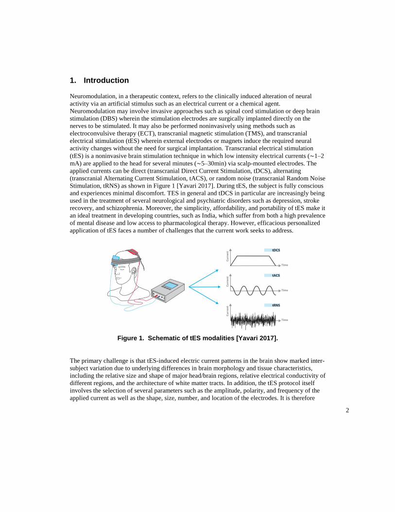
activity changes without the need for surgical implantation. Transcranial electrical stimulation
(tES) is a noninvasive brain stimulation technique in which low intensity electrical currents (∼1–2
mA) are applied to the head for several minutes (∼5–30min) via scalp-mounted electrodes. The
applied currents can be direct (transcranial Direct Current Stimulation, tDCS), alternating
(transcranial Alternating Current Stimulation, tACS), or random noise (transcranial Random Noise
Stimulation, tRNS) as shown in Figure 1 [Yavari 2017]. During tES, the subject is fully conscious
and experiences minimal discomfort. TES in general and tDCS in particular are increasingly being
used in the treatment of several neurological and psychiatric disorders such as depression, stroke
recovery, and schizophrenia. Moreover, the simplicity, affordability, and portability of tES make it
an ideal treatment in developing countries, such as India, which suffer from both a high prevalence
of mental disease and low access to pharmacological therapy. However, efficacious personalized
application of tES faces a number of challenges that the current work seeks to address.
Figure 1. Schematic of tES modalities [Yavari 2017].
The primary challenge is that tES-induced electric current patterns in the brain show marked inter-
subject variation due to underlying differences in brain morphology and tissue characteristics,
including the relative size and shape of major head/brain regions, relative electrical conductivity of
different regions, and the architecture of white matter tracts. In addition, the tES protocol itself
involves the selection of several parameters such as the amplitude, polarity, and frequency of the
applied current as well as the shape, size, number, and location of the electrodes. It is therefore

3
difficult to predict the distribution of electric current in the brain and consequently the likely
efficacy of the treatment for a particular subject. Computational modeling and simulation of tES
can potentially address this challenge. By computing the resulting electric field with high spatial
resolution, we can observe exactly which brain regions are likely to have been stimulated and thus
correlate input (treatment protocol) parameters with output (clinical or behavioral outcomes).
Moreover, by virtually experimenting with different treatment protocols on a subject-specific
simulation model, the clinician can determine the most efficacious treatment for a given individual
rather than relying on conventional nonspecific guidelines as is typically the case today.
2. Simulation Workflow for tDCS in Schizophrenia
2.1 Neurophysiology of tDCS in Treatment of Schizophrenia
Schizophrenia is a serious mental disorder characterized by incoherent or illogical thoughts and
bizarre behavior and speech. Positive symptoms include delusions and hallucinations, while
negative symptoms include emotional withdrawal, difficulty in abstract thinking, and lack of
spontaneity. Positive symptoms are associated with excessive neural activation in the temporo-
parietal junction, while negative symptoms are associated with deficient neural activation in the
prefrontal cortex (Figure 2). Since neuronal activation is positively correlated with membrane
potential, tDCS works by applying an anodic stimulation to the underactivated brain regions to
increase the local resting potential (i.e., depolarization) and applying a cathodic stimulation to the
overactive brain regions to decrease the resting potential (i.e., hyperpolarization) in that
neighborhood. Note that tDCS does not directly generate a neuronal action potential, rather, it
increases or decreases neuronal excitability or the probability that an action potential will be
spontaneously triggered by normal synaptic inputs. In a typical 2-electrode tDCS protocol, a
current of 1-2mA is applied continually for 20 minutes, and a single treatment course involves 2
sessions daily for 5 days. A course of tDCS can significantly reduce auditory verbal hallucinations
(the focus of our study) for up to 3 months [Bose 2017].
Figure 2. Brain Abnormalities associated with Schizophrenia [Venkatasubramanian 2005a and 2005b].

4
2.2 Personalized Model Generation
Since the primary goal of this project was to demonstrate the value of simulation for subject-
specific tDCS outcome prediction, a post-hoc study was conducted to analyze the results of two
patients with persistent auditory verbal hallucinations despite antipsychotic medication. One
patient had responded favorably to tDCS while the other had not even though both were
administered identical treatments (i.e., electrode positions, input currents, duration, etc.). The
objective of the study was to examine if simulation could shed light on the difference in outcomes.
To begin, T1 weighted MRI scans for the subjects were acquired using a Philips Ingenia 3T
scanner with 1mm3 resolution. Each scan was then segmented using a probabilistic segmentation
procedure with the Statistical Parametric Mapping (SPM) toolkit [Ashburner 2005] into 6 distinct
non-overlapping tissue regions: grey matter (GM), white matter (WM), cerebrospinal fluid (CSF),
skin/flesh, skull, and sinus/air. Segmentation errors (e.g., non-smooth tissue surfaces and
disconnected regions) were corrected using automated routines in MATLAB® [Huang 2012].
After a satisfactory 3D head/brain model was developed, electrode placement was performed with
Simpleware® ScanIP (+ ScanCAD module) using the 10/10 international convention with the
anode at AF3 and the cathode at CP5 (Figure 3). Finally a high resolution tetrahedral FE mesh
(average element size = 1mm3) was generated using the ScanIP (+ ScanFE) module.
Figure 3. International 10/10 Convention showing Anode AF3 (red) and Cathode CP5 (blue); Subject-specific Models (Left: Responder; Right: Non-responder).
2.3 FE Analysis: Scenario
Each FE model (responder and non-responder) was meshed with about 3M nodes and 17M
DC3D4E electrical conduction elements. The different brain regions were assigned appropriate
isotropic electrical conductivity values taken from the literature (shown in Figure 4). A thin layer
of gel was also included in the model between the scalp and the electrodes to better mimic the
experimental set-up. At the anode, an inward current of 2mA was applied while at the cathode an
outward current of 2mA was applied; the rest of the exterior surface of the model was insulated.
At an arbitrary node of the model in the chin region (away from the electrodes), the electric

5
potential was set to zero to eliminate possible rigid body solutions. A single-step single-increment
electrical analysis was performed in Abaqus/Standard version R2017x to determine the electrical
potential gradient (EPG) distribution (which is identical to the electric current density distribution)
in the brain. The different tissue regions and material properties used are shown in Figure 4.
Figure 4. FE Model Regions (Responder) and Conductivities (both Subjects).
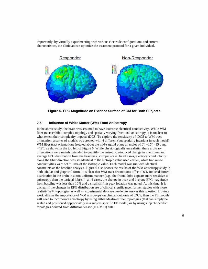
2.4 FE Analysis: Results
By examining the distribution of electric current at steady state, we can see that overall head shape
and tissue morphology play an important role in determining the focus of neurostimulation in a
specific subject. Careful comparison of the EPG distribution on the exterior surface of the grey
matter (GM) (Figure 5) shows a higher electric current density in the parietal lobe of the
responder, while in the non-responder, we see current more evenly distributed across the parietal
and frontal lobes. This can be explained by the fact that the responder’s grey matter contains
deeper sulci in the parietal lobe when compared with those seen in the non-responder. As the sulci
are filled with CSF, which is a better conductor than grey matter, we can expect the current
density to be higher in this region for the responder than for the non-responder. Since the total
current in the brain is the same in both cases (2mA), this could imply that the parietal regions,
implicated in auditory hallucinations, are being insufficiently stimulated in the case of the non-
responder rendering his treatment less efficacious. Possible solutions include increasing the
amplitude of the current, repositioning the electrodes, or using multiple electrodes to focus the
current more effectively at the temporo-parietal junction. We also see very low (physiologically
insignificant) electric current density in regions below the WM/GM boundary as expected. From
this simple retrospective analysis, we can see how subject-specific 3D electric current distribution
information can explain (at least partially) the difference in response between subjects. More
6
importantly, by virtually experimenting with various electrode configurations and current
characteristics, the clinician can optimize the treatment protocol for a given individual.
Figure 5. EPG Magnitude on Exterior Surface of GM for Both Subjects
2.5 Influence of White Matter (WM) Tract Anisotropy
In the above study, the brain was assumed to have isotropic electrical conductivity. While WM
fiber tracts exhibit complex topology and spatially varying fractional anisotropy, it is unclear to
what extent their complexity impacts tDCS. To explore the sensitivity of tDCS to WM tract
orientation, a series of models was created with 4 different (but spatially invariant in each model)
WM fiber tract orientations (rotated about the mid-sagittal plane at angles of 0o, +15
o, -15
o, and
+45o), as shown in the top left of Figure 6. While physiologically unrealistic, these arbitrary
orientations were mainly intended to quantify the anisotropy-induced change in maximum and
average EPG distribution from the baseline (isotropic) case. In all cases, electrical conductivity
along the fiber direction was set identical to the isotropic value used earlier, while transverse
conductivities were set to 10% of the isotropic value. Each model was run with identical
constraints as the baseline analysis. Figure 6 also shows the results of the WM anisotropy study in
both tabular and graphical form. It is clear that WM tract orientations affect tDCS-induced current
distribution in the brain in a non-uniform manner (e.g., the frontal lobe appears more sensitive to
anisotropy than the parietal lobe). In all 4 cases, the change in peak and average EPG magnitude
from baseline was less than 10% and a small shift in peak location was noted. At this time, it is
unclear if the changes in EPG distribution are of clinical significance; further studies with more
realistic WM topologies as well as experimental data are needed to answer this question. If future
work affirms the importance of WM anisotropy on clinical outcome of tDCS, then the FE models
will need to incorporate anisotropy by using either idealized fiber topologies (that can simply be
scaled and positioned appropriately in a subject-specific FE model) or by using subject-specific
topologies derived from diffusion tensor (DT-MRI) data.

7
Figure 6. Models and Results from WM Anisotropy study.
3. Noninvasive Deep Brain Stimulation
3.1 Limitations of tDCS for Deep Brain Stimulation
While tDCS is increasingly being used in clinical settings, its applicability is predominantly
limited to disorders that originate in malfunctions of the higher regions of the brain, primarily in
the cortex. This is because tDCS uses low intensity currents that are unable to penetrate into the
deeper regions of the brain (although deep brain regions may be indirectly modulated due to
neural network connectivity). Increasing current amplitude will allow deeper regions to be
stimulated but may be undesirable for two reasons. First, greater current strength will also
stimulate normally functioning overlying areas and may even cause unintended neuronal firing.
Second, prolonged exposure to higher current can cause discomfort or injury to the scalp. The
conventional treatment for deep brain disorders therefore uses deep brain stimulation (DBS)
wherein stimulation electrodes are surgically implanted directly into the malfunctioning areas so
that neuromodulation can be limited to a small area with minimal disruption of the surrounding
tissue. However, DBS is a highly invasive procedure with potential adverse effects including
electrode displacement and erosion, infection, stroke, and seizures. Moreover, the high cost of
DBS surgery and recovery, and the high level of clinical expertise necessary to ensure positive
outcomes typically render this treatment infeasible for routine public health in developing
countries such as India. Recent research suggests that tES may be a viable alternative to
conventional DBS, at least for some mental disorders. The second part of our work describes how
tES can be used for subject-specific noninvasive DBS and extends our computational workflow to
facilitate clinical use of this new technology.
3.2 Transcranial Alternating Current Stimulation (tACS)
While some mental disorders involve abnormal (and polarity-specific) neuronal excitability and
can therefore be treated by the application of direct current, others, such as Parkinson’s disease,

8
Alzheimer’s and epilepsy are correlated with abnormal brain rhythms (which typically range from
0.05Hz to 500Hz) [Reato 2013]. Treatments for these conditions may therefore involve attempts to
restore normal brain wave activity in the affected area using alternating current. AC stimulation
can improve brain rhythm either by entrainment (where brain oscillation frequency is aligned with
the forcing frequency) or by modulation (where brain oscillation amplitude is scaled by the
external signal) as shown in Figure 7 [Reato 2013].
Figure 7. Effects of AC stimulation on Brain Oscillation [Reato 2013].
3.3 Temporal Interference in tACS
If the malfunctioning neurons are located in deep brain structures, then “conventional” application
of tACS via scalp electrodes will suffer from the same limitations as those outlined for tDCS.
However, as demonstrated by Grossman et al [Grossman 2017], if we use two frequencies instead
of one, it becomes possible to selectively stimulate the deep brain without affecting the
surrounding tissue by exploiting the phenomenon of wave interference. Consider two electric
fields Ē1 and Ē2 of equal magnitude that coexist at the same point in space. If the two fields
oscillate at slightly different frequencies (f1 and f2 = f1+∆f), the resultant linearly superposed field
will oscillate at the average frequency (f1+ f2)/2 but its amplitude will be modulated at the
difference or ‘beat’ frequency ∆f. Moreover, the beat amplitude will depend on the degree of
alignment of the two fields Ē1 and Ē2. This is illustrated in Figure 8 – on the left side, we see that
the envelope of the y-component of resultant modulated field ĒAM = Ē1 + Ē2 has a high amplitude
if the y-components of Ē1 and Ē2 have similar magnitudes, whereas the reverse is true if their y-
components have dissimilar magnitudes. The net amplitude of the modulated signal ĒAM at any
point in space is the vector sum of the amplitudes of the x-, y-, and z-components of ĒAM.
The main point of this discussion is that if it were possible to specify Ē1 and Ē2 at every point in
some closed domain, we would be able to control the amplitude of the resultant linearly
superposed field throughout the domain. In regions where a high amplitude envelope was desired,
we would need to ensure close alignment in the magnitude and direction of the individual fields Ē1
and Ē2, whereas in regions where minimal or no modulation was desired, we could have one field
be much stronger than the other. For the simple 2D case of a closed circular domain, this concept
is illustrated on the right side of Figure 8 where we can see that Ē1 and Ē2 are aligned and of equal
magnitude in the central region of the domain. Therefore the beat amplitude would be highest in
this region and would gradually decrease as we move away from it. This concept of linearly
superposing two oscillating electric fields (also known as temporal interference) suggests a
technique to stimulate specific structures of the brain with minimal impact on other structures.

9
Figure 8. Temporal Interference in tACS [Grossman 2017].
3.4 Neurophysiology of Temporal Interference in tACS
Temporal Interference tACS (TI-tACS) relies on two important neurophysiological characteristics.
The first is that neurons respond to low frequency external fields but their response decreases
significantly at high frequencies. In essence, the neuron acts as a low-pass filter that is effectively
insensitive to frequencies above some threshold (typically ~1kHz). Moreover, greater the
amplitude of the local excitation, greater is the neuronal response. In Figure 9 [Reato 2013], we
see that membrane polarization (i.e., the response of the neuron) decreases as the frequency of the
applied AC signal increases and increases with increasing AC signal amplitude. Therefore, if we
set the frequency of both signals (Ē1 and Ē2) above the threshold, we will stimulate only those
regions in the brain where the two fields result in a modulated signal of appreciable amplitude. In
other regions, the modulated amplitude will be too low and the average frequency too high to
effect any change in the neurons. As such, we can selectively stimulate the brain using TI-tACS.
Figure 9. Effects of AC stimulation on Single Neurons [Reato 2013].
10
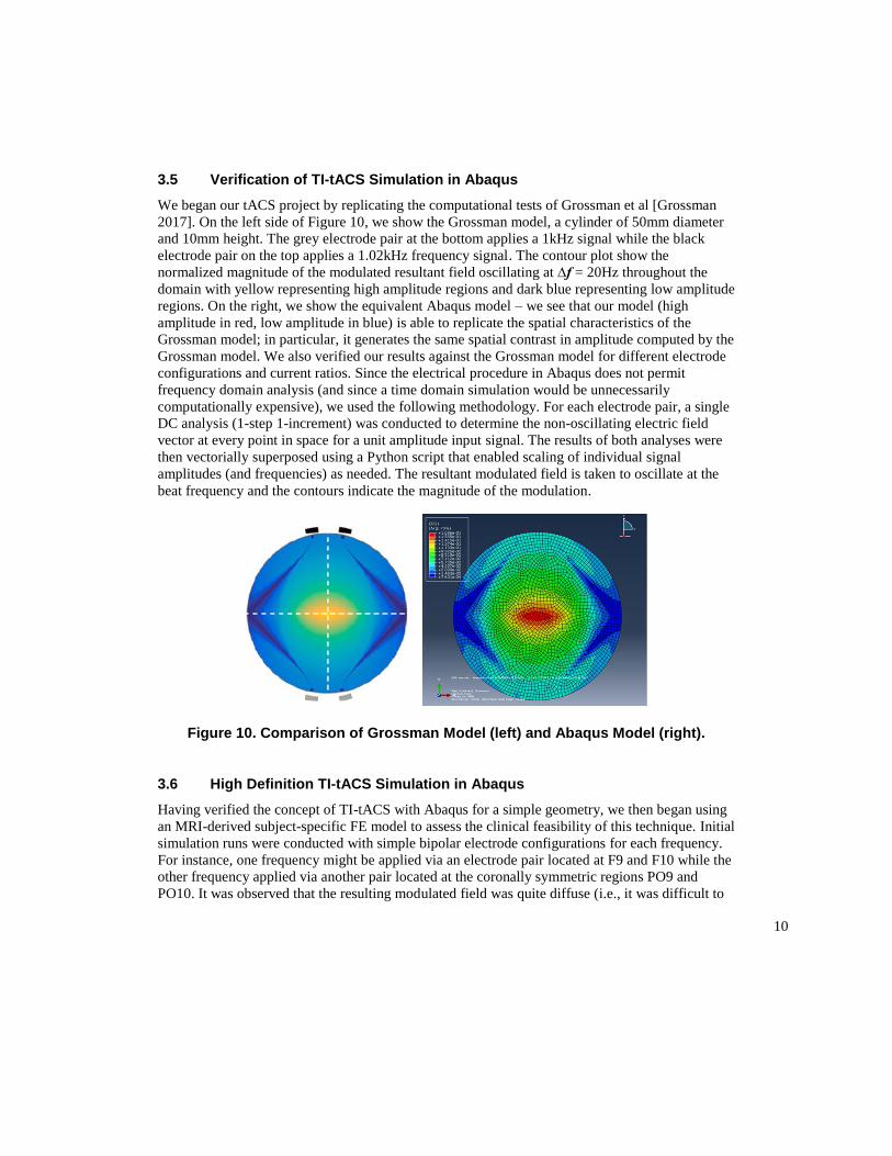
3.5 Verification of TI-tACS Simulation in Abaqus
We began our tACS project by replicating the computational tests of Grossman et al [Grossman
2017]. On the left side of Figure 10, we show the Grossman model, a cylinder of 50mm diameter
and 10mm height. The grey electrode pair at the bottom applies a 1kHz signal while the black
electrode pair on the top applies a 1.02kHz frequency signal. The contour plot show the
normalized magnitude of the modulated resultant field oscillating at ∆f = 20Hz throughout the
domain with yellow representing high amplitude regions and dark blue representing low amplitude
regions. On the right, we show the equivalent Abaqus model – we see that our model (high
amplitude in red, low amplitude in blue) is able to replicate the spatial characteristics of the
Grossman model; in particular, it generates the same spatial contrast in amplitude computed by the
Grossman model. We also verified our results against the Grossman model for different electrode
configurations and current ratios. Since the electrical procedure in Abaqus does not permit
frequency domain analysis (and since a time domain simulation would be unnecessarily
computationally expensive), we used the following methodology. For each electrode pair, a single
DC analysis (1-step 1-increment) was conducted to determine the non-oscillating electric field
vector at every point in space for a unit amplitude input signal. The results of both analyses were
then vectorially superposed using a Python script that enabled scaling of individual signal
amplitudes (and frequencies) as needed. The resultant modulated field is taken to oscillate at the
beat frequency and the contours indicate the magnitude of the modulation.
Figure 10. Comparison of Grossman Model (left) and Abaqus Model (right).
3.6 High Definition TI-tACS Simulation in Abaqus
Having verified the concept of TI-tACS with Abaqus for a simple geometry, we then began using
an MRI-derived subject-specific FE model to assess the clinical feasibility of this technique. Initial
simulation runs were conducted with simple bipolar electrode configurations for each frequency.
For instance, one frequency might be applied via an electrode pair located at F9 and F10 while the
other frequency applied via another pair located at the coronally symmetric regions PO9 and
PO10. It was observed that the resulting modulated field was quite diffuse (i.e., it was difficult to

11
generate focused amplification of the modulated signal). Moreover, in some cases, we observed
constructive interference in multiple disconnected regions (i.e., off-target locations were being
stimulated as effectively as the target location). Both issues can be seen in Figure 11 for the
configuration mentioned above. To circumvent these problems, we decided to deploy multipolar
electrode configurations, also known as High Definition tACS (HD-tACS) in which more than 2
electrodes are used for each frequency. We used a 4x1 multipolar configuration as shown in
Figure 12. For both frequencies (1kHz and 1.02kHz), the polarity of the center electrode
(highlighted in yellow) is opposite to that of the four surrounding electrodes and the applied
currents are scaled accordingly (e.g., +1mA for the central electrode, -0.25mA for each of the
surrounding electrodes in the Abaqus DC analysis).
Figure 11. TI-tACS Simulation using an Electrode Pair for each Frequency.
Figure 12. High Definition 4x1 Montage used for TI-tACS Simulations.
12
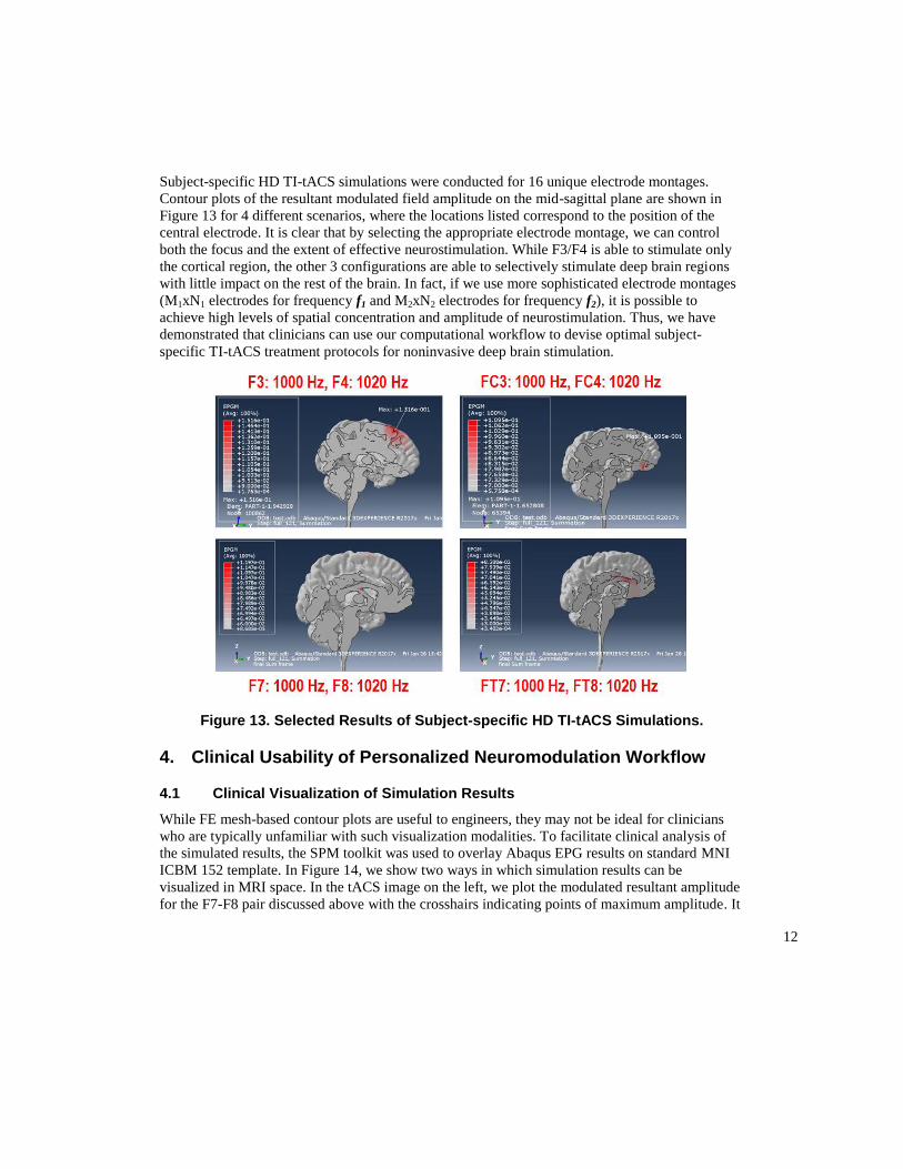
Subject-specific HD TI-tACS simulations were conducted for 16 unique electrode montages.
Contour plots of the resultant modulated field amplitude on the mid-sagittal plane are shown in
Figure 13 for 4 different scenarios, where the locations listed correspond to the position of the
central electrode. It is clear that by selecting the appropriate electrode montage, we can control
both the focus and the extent of effective neurostimulation. While F3/F4 is able to stimulate only
the cortical region, the other 3 configurations are able to selectively stimulate deep brain regions
with little impact on the rest of the brain. In fact, if we use more sophisticated electrode montages
(M1xN1 electrodes for frequency f1 and M2xN2 electrodes for frequency f2), it is possible to
achieve high levels of spatial concentration and amplitude of neurostimulation. Thus, we have
demonstrated that clinicians can use our computational workflow to devise optimal subject-
specific TI-tACS treatment protocols for noninvasive deep brain stimulation.
Figure 13. Selected Results of Subject-specific HD TI-tACS Simulations.
4. Clinical Usability of Personalized Neuromodulation Workflow
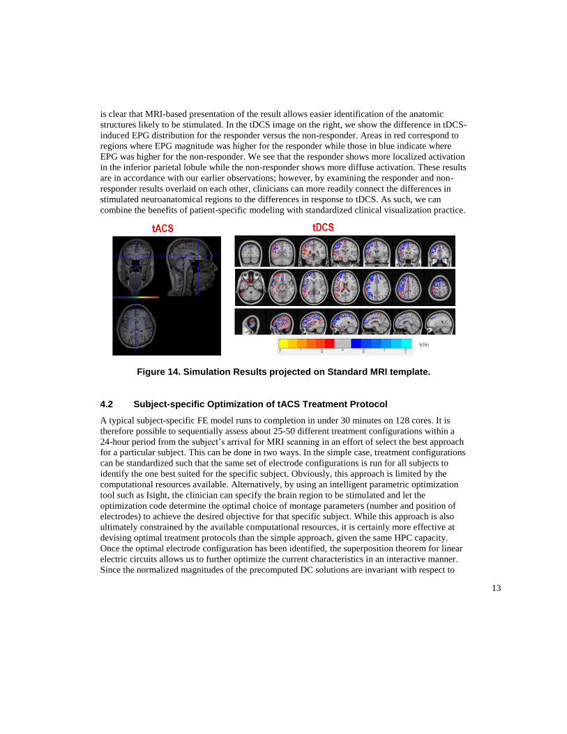
4.1 Clinical Visualization of Simulation Results
While FE mesh-based contour plots are useful to engineers, they may not be ideal for clinicians
who are typically unfamiliar with such visualization modalities. To facilitate clinical analysis of
the simulated results, the SPM toolkit was used to overlay Abaqus EPG results on standard MNI
ICBM 152 template. In Figure 14, we show two ways in which simulation results can be
visualized in MRI space. In the tACS image on the left, we plot the modulated resultant amplitude
for the F7-F8 pair discussed above with the crosshairs indicating points of maximum amplitude. It
13
is clear that MRI-based presentation of the result allows easier identification of the anatomic
structures likely to be stimulated. In the tDCS image on the right, we show the difference in tDCS-
induced EPG distribution for the responder versus the non-responder. Areas in red correspond to
regions where EPG magnitude was higher for the responder while those in blue indicate where
EPG was higher for the non-responder. We see that the responder shows more localized activation
in the inferior parietal lobule while the non-responder shows more diffuse activation. These results
are in accordance with our earlier observations; however, by examining the responder and non-
responder results overlaid on each other, clinicians can more readily connect the differences in
stimulated neuroanatomical regions to the differences in response to tDCS. As such, we can
combine the benefits of patient-specific modeling with standardized clinical visualization practice.
Figure 14. Simulation Results projected on Standard MRI template.
4.2 Subject-specific Optimization of tACS Treatment Protocol
A typical subject-specific FE model runs to completion in under 30 minutes on 128 cores. It is
therefore possible to sequentially assess about 25-50 different treatment configurations within a
24-hour period from the subject’s arrival for MRI scanning in an effort of select the best approach
for a particular subject. This can be done in two ways. In the simple case, treatment configurations
can be standardized such that the same set of electrode configurations is run for all subjects to
identify the one best suited for the specific subject. Obviously, this approach is limited by the
computational resources available. Alternatively, by using an intelligent parametric optimization
tool such as Isight, the clinician can specify the brain region to be stimulated and let the
optimization code determine the optimal choice of montage parameters (number and position of
electrodes) to achieve the desired objective for that specific subject. While this approach is also
ultimately constrained by the available computational resources, it is certainly more effective at
devising optimal treatment protocols than the simple approach, given the same HPC capacity.
Once the optimal electrode configuration has been identified, the superposition theorem for linear
electric circuits allows us to further optimize the current characteristics in an interactive manner.
Since the normalized magnitudes of the precomputed DC solutions are invariant with respect to
14
changes in amplitude or frequency, we can modify these parameters for each field individually and
examine the resultant current distribution in real time. This allows the clinician to fine tune the
current characteristics to achieve more focused neurostimulation. For instance, by retaining the
optimal electrode positions but modifying the amplitude ratio of the two input frequencies, the
clinician can shift the focal point in real time (using visual feedback for guidance). This two-step
optimization of subject-specific tACS treatment protocols is illustrated in Figure 15.
Figure 15. Two-step Methodology to Optimize Subject-specific tACS Treatment.
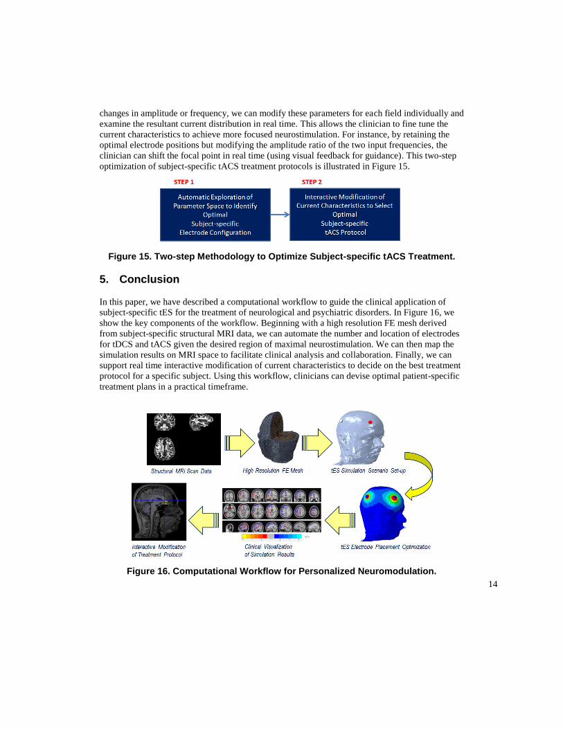
5. Conclusion
In this paper, we have described a computational workflow to guide the clinical application of
subject-specific tES for the treatment of neurological and psychiatric disorders. In Figure 16, we
show the key components of the workflow. Beginning with a high resolution FE mesh derived
from subject-specific structural MRI data, we can automate the number and location of electrodes
for tDCS and tACS given the desired region of maximal neurostimulation. We can then map the
simulation results on MRI space to facilitate clinical analysis and collaboration. Finally, we can
support real time interactive modification of current characteristics to decide on the best treatment
protocol for a specific subject. Using this workflow, clinicians can devise optimal patient-specific
treatment plans in a practical timeframe.
Figure 16. Computational Workflow for Personalized Neuromodulation.

15
Future work on this project will include both scientific and practical components. To deploy this
workflow at scale in a clinical setting, the Image->Mesh process needs to be robust and fully
automated. More research needs to be done on TI-tACS, HD electrode configurations, and the
effects of electrical anisotropy of the brain. We are currently developing a multiscale methodology
to couple single neuron biophysics (systems) models to 3D whole brain (FE) models to elucidate
the neurophysiological changes induced by tES. We are also using machine learning to develop a
more holistic predictive framework based on 3D imaging and physics-based simulation as well as
on subject-specific genetic, clinical, biometric, behavioral, and environmental information to
better guide the diagnosis and treatment of neurological and psychiatric disorders.
6. Acknowledgments
This work was supported by the Swarnajayanti Fellowship Research Grant (DST/SJF/LSA-
02/2014-15) awarded by the Department of Science and Technology (Government of India) to Dr.
Ganesan Venkatasubramanian. UberCloud, Advania, Hewlett Packard Enterprise, and Intel
provided cloud-based HPC resources for verification of subject-specific TI-tACS optimization.
7. References
1. Ashburner, J., K. J. Friston, “Unified Segmentation,” Neuroimage, Volume 26, 2005
2. Bose, A., V. Shivakumar, S. M. Agarwal, S. V. Kalmady, S. Shenoy, V. S. Sreeraj, et al,
“Efficacy of Fronto-temporal Transcranial Direct Current Stimulation for Refractory Auditory
Verbal Hallucinations in Schizophrenia: A Randomized, Double-blind, Sham-controlled
Study,” Schizophrenia Research, 2017 (in press)
3. Grossman, N., D. Bono, N. Dedic, S. Kodandaramaiah, A. Rudenko, H-J Suk, et al,
“Noninvasive Deep Brain Stimulation via Temporally Interfering Electric fields,” Cell,
Volume 169, 2017
4. Huang Y, Y. Su, C. Rorden, J. Dmochowski, A. Datta, L. C. Parra, “An Automated Method
for High-Definition Transcranial Direct Current Stimulation Modeling,” International
Conference of the IEEE Engineering in Medicine and Biology Society, 2012
5. Reato, D., A. Rahman, M. Biksom, L. C. Parra, “Effects of Weak Alternating Current
Stimulation on Brain Activity – A Review of Known Mechanisms from Animal Studies,”
Frontiers in Human Neuroscience, Volume 7, 2013
6. Venkatasubramanian, G., M. D. Hunter, S. A. Spence, “Schneiderian First-Rank Symptoms
and Right Parietal Hyperactivation: A Replication Using fMRI,” American Journal of
Psychiatry, Volume 162, 2005a
7. Venkatasubramanian G., R. D. Green, M. D. Hunter, I. D. Wilkinson, S. A. Spence,
“Expanding the Response Space in Chronic Schizophrenia: The Relevance of Left Prefrontal
Cortex,” NeuroImage, Volume 25, 2005b
8. Yavari, F., M. A. Nitsche, H. Ekhtiari, “Transcranial Electric Stimulation for Precision
Medicine: A Spatiomechanistic Framework,” Frontiers in Human Neuroscience, Volume 11,
2017