persistent arrays, path problems, and context-free … · schemata, so wie sie zum beispiel im cyk...
TRANSCRIPT
Technische Universität Darmstadt,Fachbereich Informatik.
Genehmigte Dissertation zur Erlangungdes akademischen Grades Dr. rer. nat.
Persistent Arrays,Path Problems,
and Context-free Languages
Dissertation – vorgelegt vonDipl.-Inform. Oliver Glier
geboren in Frankfurt am Main
Tag der Einreichung: 31. Januar 2005 Referenten:
Tag der mündlichen Prüfung: 21. April 2005Prof. Dr. Hermann K.-G. Walter, Darmstadt
Prof. Dr. Jürgen Albert, Würzburg
Darmstädter Dissertationen D17 Priv-Doz. Dr. Ulrike Brandt, Darmstadt


0.1 Deutschsprachige Zusammenfassung
Das Ziel dieser Arbeit ist es, einen Rahmen für die Modellierung sprachbeschränkter Wegeproblemein Graphen zu schaffen. Von konzeptioneller Seite sind da kontextfreie Grammatiken und Semiringe
zu nennen. Kontextfreie Grammatiken erlauben die Beschreibung rekursiver generativer Prozesse,
wie sie beispielsweise in der Grammatik natürlicher Sprache auftauchen oder zur Beschreibung vonZellwachstum dienen können. Sie erfassen außerdem die Struktur einiger dynamischer Programmier-
schemata, so wie sie zum Beispiel im CYK Algorithmus für kontextfreies Parsing oder in manchen
pseudopolynomiellen Algorithmen für schwere Probleme benutzt werden.Die Verbindung kontextfreier Grammatiken mit Wegeproblemen in Graphen erlauben die Modellierung
zusätzlicher formalsprachlicher Einschränkungen der möglichen Wege. Auf der anderen Seite könnenkontextfreie Grammatiken analog zum algebraischen Wegeproblem mit Semiringwerten ausgestattet
werden. Im vierten Kapitel dieser Arbeit werden diese Beziehungen zwischen semiringbewerteten
kontextfreien Grammatiken und Wegeproblemen näher untersucht. Diese Verbindung ist fruchtbarund erlaubt einen konzeptionellen Rahmen für Verallgemeinerungen des Wegeproblems für Graphen,
beispielsweise zur Formulierung von Polynomialzeitalgorithmen für Transportprobleme welche sonstgar nicht oder nur umständlich als konventionelle Wegeprobleme dargestellt werden können.
Wie sich beobachten lässt, können formalsprachliche Einschränkungen dazu führen, dass dieerlaubten Wege exponentiell lang werden. Persistente Arrays, welche als binäre Bäume dargestellt
werden, erlauben mit diesem Problem umzugehen und erhalten die Eigenschaft der Polynomi-
alzeitberechenbarkeit. Allerdings wirft die Darstellung bestimmter exponentiell langer Wege inpolynomiellem Platz die Frage auf, welche Berechnungen überhaupt auf sie angewandt werden können.
Tatsächlich scheint sogar die Bestimmung, ob zwei solche Arrays äquivalent sind, schwer durchführbar
zu sein. Im dritten Kapitel zeigen wir neben anderen Algorithmen für persistente Arrays einenprobabilistischen Äquivalenztest. Persistente Arrays als solche werden bereits im ersten Kapitel kurz
vorgestellt. Dort zeigen wir auch, dass das „Zippen" zweier persistenter Arrays exponentieller Länge,welche als Bäume dargestellt werden, im Allgemeinen nicht in einer Zeit durchgeführt werden kann,
welche polynomiell zu deren Größe im Speicher wächst.
Das zweite Kapitel führt in Wegeprobleme in Graphen ein. Der erste Abschnitt befasst sich mit
Wegeproblemen in dynamischen Wäldern. Auch wenn der resultierende Algorithmus nicht so schnell
wie die bestbekannten Algorithmen ist, erlaubt er eine einfache Implementierung, falls persistenteArrays bereits in einer Programmierbibliothek vorhanden sind. Wir stellen außerdem Semiringe und
das algebraische Wegeproblem in Verbindung mit persistenten Arrays vor.
Kapitel 5. zeigt einige Ergebnisse aus der Theorie formaler Sprachen, welche sich während dieser
Arbeit ergeben haben. In Kapitel 6. zeigen wir weiterhin, wie Rytters Formulierung von Valiants subku-
i

bischem Algorithmus für kontextfreies Parsing mit Semiringparsing und Wegeproblemen in Verbindungsteht.
0.2 Preface
The goal of this thesis is to provide a framework for several path problems for graphs. From the
conceptual part, there are context-free grammars and semirings. Context-free grammars allow us todescribe recursive generative processes, such as in grammars for natural languages or in models for the
growth of cell complexes. They also capture the structure of certain dynamic programming schemes, as
it is used in the CYK algorithm for context-free parsing and of some pseudo-polynomial algorithms forhard problems.
The connection of context-free grammars with path problems in graphs allows us to model several
language-restrictions for feasible paths and thus generalizes the classic shortest-path problem. Onthe other hand — similarly to the algebraic shortest path problem — context-free grammars can
be equipped with semiring values. In chapter 4 of this thesis, we explore the relationship betweensemiring-valued context-free grammars and path problems. The connection is fruitful since it gives
us a conceptual framework for many generalizations of the path problem. For instance it allows us to
formulate tentative polynomial-time algorithms for transportation problems which cannot, or only withgreat difficulty, formulated as conventional shortest-path problems.
As one can observe, language-restrictions on paths might cause the shortest feasible paths to growexponentially. Persistent arrays, represented as balanced binary trees, allow us to deal with this problem
and still maintain polynomial-time computability. The ability to represent certain exponentially longarrays in polynomial space gives rise to the question what kind of computations they apply to. Indeed,
even determining equality for two of these arrays appears to be difficult. We provide a probabilistic
equality test in the third chapter, among other algorithms for persistent arrays. Persistent arraysthemselves are briefly introduced in the first chapter of this thesis. There, we also show that zipping two
persistent arrays (represented as trees) is generally not possible in time polynomial in its size in memory.
The second chapter sets the stage for path problems on graphs. The first section shows how shortest
paths in forests can be maintained dynamically. The resulting algorithms are somewhat slower than thebest algorithms known in the literature, but easier to implement if persistent arrays are already provided
by a programming library. We also introduce the semiring framework for path problems here.
Chapter 5. shows some results in formal language theory which are useful for our conceptual frame-
work. In chapter 6. we show how Rytter’s formulation of Valiant’s subcubic context-free parsing algo-
rithm is connected to semiring parsing and path problems.
ii

0.3 Acknowlegdements
Credit is due to many people who inspired, encouraged, and supported me during my research and dur-
ing the process of writing this thesis. First of all, I want to mention Professor Hermann Walter, who
guided my research and who gave me such an inspiring working environment. Of similar importance tomy work is Ulrike Brandt: Nearly all of my knowledge about the theory of formal languages I learned
from her and from Professor Walter. They introduced me to Kolmogorov complexity and to ValiantParsing which — as I think — lead to the most valuable results of this thesis. Without both of them this
thesis would not exist. I’m very grateful to Professor Jürgen Albert for his expertise and his patience
while going through the early drafts of my thesis. To all three of the aforementioned referees I owenumerous ideas, corrections, and critics of my work. It must have been as painful for them as it was for
me to see all my mistakes which they so kindly corrected.
I also want to mention Professor Helmut Waldschmidt and Klaus Guntermann. I was temporarily stayingwith their research group for system programming. During this semester I was introduced into various
fields of graph algorithms and much of this thesis is originated from there. I’m very glad that I wasable to work at Professor Walter’s research group for automata theory and formal languages: I want to
thank all members of this group and of the computer science department of TU Darmstadt. Especially
Elfi Steingasser, Jürgen Kilian, and Kai Renz have been truely supporting and encouraging colleaguesduring all this time. It is very sad to realize that this group does not exist anymore.
This work would never have been completed without the driving force of my friends Lars Bindzus andNima Barraci. They both helped me to get my English into a readable form. The layout of this thesis is
due to Lars Bindzus who made an ambitious job with a great result.
The DAAD provided me with a generous scholarship for conducting initial parts of my research atFakultas Ilmu Komputer at Universitas Indonesia. I want to thank Dr. Chan Basaruddin and my col-
leagues from Fakultas Ilmu Komputer for the opportunity to work there.
Last but not least I thank Betti Said and my parents Helga and Arthur Glier for their enduring supportand patience in all these years.
iii

iv

Contents
0.1 Deutschsprachige Zusammenfassung . . . . . . . . . . . . . . . . . . . . . . . . . . . i
0.2 Preface . . . . . . . . . . . . . . . . . . . . . . . . . . . . . . . . . . . . . . . . . . ii
0.3 Acknowlegdements . . . . . . . . . . . . . . . . . . . . . . . . . . . . . . . . . . . . iii
1 Introduction 11.1 Strings and Arrays . . . . . . . . . . . . . . . . . . . . . . . . . . . . . . . . . . . . 1
1.2 Fully Persistent Arrays . . . . . . . . . . . . . . . . . . . . . . . . . . . . . . . . . . 4
1.3 Examples for Applications . . . . . . . . . . . . . . . . . . . . . . . . . . . . . . . . 5
1.3.1 Programming Languages . . . . . . . . . . . . . . . . . . . . . . . . . . . . . 6
1.3.2 Language Restricted Path Problems . . . . . . . . . . . . . . . . . . . . . . . 6
1.4 The ADT Persistent Array . . . . . . . . . . . . . . . . . . . . . . . . . . . . . . . . 7
1.4.1 The Interface . . . . . . . . . . . . . . . . . . . . . . . . . . . . . . . . . . . 8
1.4.2 An Implementation of Persistent Arrays as Balanced Trees . . . . . . . . . . . 9
1.4.3 Homomorphisms on the Free Monoid . . . . . . . . . . . . . . . . . . . . . . 14
1.4.4 Impossibility of Pairing . . . . . . . . . . . . . . . . . . . . . . . . . . . . . . 16
1.5 Related Work . . . . . . . . . . . . . . . . . . . . . . . . . . . . . . . . . . . . . . . 19
2 Graph Algorithms and Persistent Arrays 212.1 Paths in Dynamic Trees and Forests . . . . . . . . . . . . . . . . . . . . . . . . . . . 22
2.1.1 Path Queries on Static Trees . . . . . . . . . . . . . . . . . . . . . . . . . . . 23
2.1.2 Path Queries on Dynamic Trees . . . . . . . . . . . . . . . . . . . . . . . . . 25
2.1.3 Diameter, Center, and Diameter Path . . . . . . . . . . . . . . . . . . . . . . . 29
2.2 The Semiring Framework for Shortest Paths . . . . . . . . . . . . . . . . . . . . . . . 31
2.2.1 All-Pairs-Shortest-Distance . . . . . . . . . . . . . . . . . . . . . . . . . . . 32
2.2.2 Semirings for Paths . . . . . . . . . . . . . . . . . . . . . . . . . . . . . . . . 33
2.3 All Pairs-Shortest-Paths and Successor Matrices . . . . . . . . . . . . . . . . . . . . . 37
2.4 Related Work . . . . . . . . . . . . . . . . . . . . . . . . . . . . . . . . . . . . . . . 39
3 Homomorphisms on Arrays 413.1 Algorithms on Large Arrays . . . . . . . . . . . . . . . . . . . . . . . . . . . . . . . 41
3.1.1 Polynomial Evaluation and Inequality Tests . . . . . . . . . . . . . . . . . . . 41
v
3.1.2 Lexicographic Comparison . . . . . . . . . . . . . . . . . . . . . . . . . . . . 45
3.1.3 Equality Tests for Arrays which May Contain Arrays . . . . . . . . . . . . . . 45
3.1.4 Sorting of Elements . . . . . . . . . . . . . . . . . . . . . . . . . . . . . . . 46
3.1.5 Generalized State Machine and Acceptor . . . . . . . . . . . . . . . . . . . . 46
3.2 Algorithm Design . . . . . . . . . . . . . . . . . . . . . . . . . . . . . . . . . . . . . 47
3.2.1 Poisson Trials . . . . . . . . . . . . . . . . . . . . . . . . . . . . . . . . . . . 47
3.2.2 Interactive Line Breaking . . . . . . . . . . . . . . . . . . . . . . . . . . . . . 52
3.2.3 Related Work . . . . . . . . . . . . . . . . . . . . . . . . . . . . . . . . . . . 53
4 Language-Restrictions and Minimal Syntax-Trees 554.1 Semiring-Valued Context-Free Grammars . . . . . . . . . . . . . . . . . . . . . . . . 56
4.2 Language-Restrictions and Minimum Syntax-Tree . . . . . . . . . . . . . . . . . . . . 58
4.2.1 Reducing the CF-APSD Problem to the APMS Problem . . . . . . . . . . . . 59
4.3 Solving The All-Pairs-Minimum-Syntax-Tree Problem . . . . . . . . . . . . . . . . . 61
4.3.1 Finite Languages . . . . . . . . . . . . . . . . . . . . . . . . . . . . . . . . . 64
4.4 Applications . . . . . . . . . . . . . . . . . . . . . . . . . . . . . . . . . . . . . . . . 66
4.4.1 Combinatorial Path Problems . . . . . . . . . . . . . . . . . . . . . . . . . . 67
4.4.2 Transportation Problems . . . . . . . . . . . . . . . . . . . . . . . . . . . . . 67
4.4.3 Algebraic Minimum Syntax-Tree . . . . . . . . . . . . . . . . . . . . . . . . 68
4.4.4 Deriving Pseudo-polynomial Algorithms . . . . . . . . . . . . . . . . . . . . 68
4.5 Related Work . . . . . . . . . . . . . . . . . . . . . . . . . . . . . . . . . . . . . . . 70
5 Results from Formal Language Theory 715.1 Permutations of Strings . . . . . . . . . . . . . . . . . . . . . . . . . . . . . . . . . . 71
5.2 Associativity and Regularity . . . . . . . . . . . . . . . . . . . . . . . . . . . . . . . 74
5.3 Kolmogorov Complexity and Deterministic Context-Freeness . . . . . . . . . . . . . . 77
5.3.1 A Short Introduction into Kolmogorov Complexity . . . . . . . . . . . . . . . 77
5.3.2 The KC-DCF Lemma . . . . . . . . . . . . . . . . . . . . . . . . . . . . . . 79
5.4 Related Work . . . . . . . . . . . . . . . . . . . . . . . . . . . . . . . . . . . . . . . 84
6 Valiant Parsing 876.1 Semiring Parsing and Transitive Matrix Closures . . . . . . . . . . . . . . . . . . . . 88
6.2 Transitive Closure via Shortest Paths . . . . . . . . . . . . . . . . . . . . . . . . . . . 91
6.2.1 Bottom-Up Properties . . . . . . . . . . . . . . . . . . . . . . . . . . . . . . 91
6.2.2 Strongly Congruent Grids and Shortest Paths . . . . . . . . . . . . . . . . . . 93
6.3 Applications . . . . . . . . . . . . . . . . . . . . . . . . . . . . . . . . . . . . . . . . 99
6.4 Related Work . . . . . . . . . . . . . . . . . . . . . . . . . . . . . . . . . . . . . . . 100
A Definitions from Graph Theory 101
vi

B Deamortized Bothsided Extendible Arrays 103
vii

viii

Chapter 1
Introduction
An indexed sequence of data elements a[0],a[1], . . . a[n−1] is often called “array" (throughout this the-
sis, array indices start at 0). A set of subsequent memory cells is a possible implementation of an array,
which is often used in imperative programming languages. However, in this thesis an array is consid-ered as an abstract data type. An interface for an abstract data type of dynamic arrays will be described
in section 1.4. Almost every non-trivial program uses arrays of some form: Even the most basic datastructures of every programming environment like strings, arrays, lists, stacks, queues, etc. can all be
understood as instances of arrays. From one perspective, one can regard an array as an abstract data
type, which allows to store, access, and modify the elements of a given array. From an implementation-specific perspective, arrays are a way of arranging elements in form of a data structure such that those
operations can be performed efficiently.In this introductory chapter we will make this distinction more precise. Furthermore, we will discuss
so-called persistent arrays and their standard implementation in form of binary trees. Operations on
persistent arrays are non-destructive, i.e. they leave old versions unaltered — including concatenationand splitting. This has a remarkable consequence for the representation of the underlying trees in mem-
ory: Through multiple references of inner nodes, common subarrays might be shared multiple times
among arrays or within the very same array. Particularly, it is possible to represent arrays of exponentiallength within a polynomial amount of memory. Later in the fourth chapter — during the discussion
of the language restricted path problem — we will see that this remarkable property is indeed useful.That is, there are applications where exponentially long arrays emerge naturally during the course of
computation. In this chapter, we give time bounds for machines equipped with array operations for
concatenation and splitting, and we also show how information can be extracted from arrays in terms ofhomomorphic images.
1.1 Strings and Arrays
We start with an example: A typical programming task is to map a string to another string. String
processing is so important that entire programming languages have been designed with this purpose in
1

Introduction
mind, for instance the language Perl. Almost all programming languages offer some representation ofstrings as a primitive type in some way, or at least as a fundamental part of their programming libraries.
Consider the task of being given a string v ∈ X ∗ of length n, where all symbols x0, . . . ,xn−1 ofv = x0 · · ·xn−1 are taken from the set X = 0,1,2, . . . ,k− 1. Now, additionally given a family of
strings si ∈ X∗, i = 0..k− 1, the task is to compute the image of v under the substitution i 7→ s i, i.e., to
generate the string sx(1) · · · sx(n). The task is not difficult, but has some pitfalls if implemented naively.
Before considering any code, some words on notation first: If not stated otherwise, all strings are
considered to be finite sequences (also called words). Usually, the letters X ,Y, . . . denote the set ofpossible symbols of the strings in consideration. The set of all strings over X is denoted by X ∗, which
together with concatenation · and the empty string ε forms the free monoid over X . We prefer to usethe term “string” instead of “word”. When writing programs which operate on strings or on any other
mathematically well-defined object, we must distinguish
1. the abstract data type which corresponds to the mathematical object “string” including all required
operations on it, and
2. the data structures and algorithms that implement the abstract data type.
In order to make this distinction clear, we present a program of our introductory programming task:
Algorithm 1.1 simultaneous string substitutionv is array of 0..k−1
s is array[0..k−1] of array of 0..k−1v := ReadLine()
n := length(v)
for i = 0..k−1 dos[i] := ReadLine()
end for
v′ is array of 0..k−1
v′ := emptyArrayfor i = 0..n−1 do
v′ := v′ · v[s[i]]
end forreturn v′
For all code in this thesis, we use a pseudo programming language, which is similar to C or Pascal
and which is not explained any further. Whenever necessary, some remarks will hopefully make the
meaning clear: In this example, all strings are implemented as arrays of unbounded size, while the
2

1.1 Strings and Arrays
family of strings si, i = 0..k−1 is implemented as a fixed-size array of strings. After reading the input,
the result v′ is computed by iterative concatenation of all v[s[i]], i = 0..n− 1. This implementation isstraightforward, so what is wrong with it? The answer depends on the underlying representation of the
data type array. In many programming languages, an array a of length n is represented by a sequenceof n subsequent memory cells. In case that the array elements have a fixed size or alternatively when
they are represented by pointers to their location in memory, then the ith element a[i] of array a can be
accessed by computing the memory address
ADDRESS[a, i] := BASEADDRESS(a) + i ·ELEMENTSIZE .
The drawback of storing an array in subsequent memory cells is that appending elements to the
array can be costly: if the subsequent memory cells behind ADDRESS(a,n−1) are already occupied byother objects, then appending a single new element requires to copy the first n elements of a to another
sufficiently large memory area. When this is done naively, then each concatenation in the program
above consumes O(n) time, even if the new strings si are negligibly short. The total running time of thealgorithm above is then O(n2).
Fortunately there are many alternative techniques for implementing extendable arrays, as we will alsodiscuss in appendix B. Those techniques usually lead to constant running time (which sometimes only
amortized) for appending a new single element.1 Now, if each of the si can be considered to have
negligible length compared to v, O(1) time for appending single elements leads to O(n) total runningtime for the program above.
After all, our program depends on an efficient implementation of the abstract data type (ADT) “array”
with operations for appending single elements to the right as well as accessing elements a[i] by theirrespective index i. The example also shows the distinction between strings as mathematical objects, and
their representation by a suitable ADT. It is sometimes worthwhile to restrict the interface of the ADTARRAY: Such restrictions may permit more efficient implementations, and also ensure correct use of the
array within the given context.
1. Stacks allow appending and removing single elements on one side.
2. Queues allow appending single elements on one side and removing single elements on the other
side.
3. Deques (Double Ended Queues) allow appending and removing single elements on both sides.
4. Lists are likewise but do not allow direct access to elements by their index. Depending on theimplementation of the lists, they have other well-known interfaces.
All four ADTs can be implemented in such a way that their operations need only constant time.
1For example the class VECTOR of the JAVA API or the deque implementation of C++ Standard Template Library (STL)
3
Introduction
In the following section we will see how the entire set of operations of the ADT ARRAY can be
implemented in such a way that each operation is sufficiently efficient. That is, all operations — in-cluding concatenation and splitting — need time logarithmic in the length of the given arrays. The
standard implementation are binary trees, which have the additional advantage of being fully persistent,i.e. operations on them do not destroy old versions of the data structure.
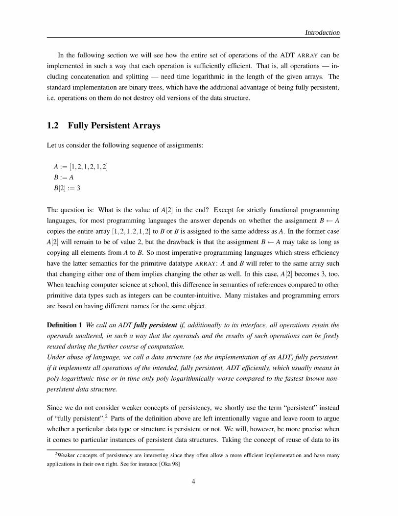
1.2 Fully Persistent Arrays
Let us consider the following sequence of assignments:
A := [1,2,1,2,1,2]
B := A
B[2] := 3
The question is: What is the value of A[2] in the end? Except for strictly functional programminglanguages, for most programming languages the answer depends on whether the assignment B← A
copies the entire array [1,2,1,2,1,2] to B or B is assigned to the same address as A. In the former caseA[2] will remain to be of value 2, but the drawback is that the assignment B← A may take as long as
copying all elements from A to B. So most imperative programming languages which stress efficiency
have the latter semantics for the primitive datatype ARRAY: A and B will refer to the same array suchthat changing either one of them implies changing the other as well. In this case, A[2] becomes 3, too.
When teaching computer science at school, this difference in semantics of references compared to other
primitive data types such as integers can be counter-intuitive. Many mistakes and programming errorsare based on having different names for the same object.
Definition 1 We call an ADT fully persistent if, additionally to its interface, all operations retain the
operands unaltered, in such a way that the operands and the results of such operations can be freely
reused during the further course of computation.
Under abuse of language, we call a data structure (as the implementation of an ADT) fully persistent,
if it implements all operations of the intended, fully persistent, ADT efficiently, which usually means in
poly-logarithmic time or in time only poly-logarithmically worse compared to the fastest known non-
persistent data structure.
Since we do not consider weaker concepts of persistency, we shortly use the term “persistent” instead
of “fully persistent”.2 Parts of the definition above are left intentionally vague and leave room to arguewhether a particular data type or structure is persistent or not. We will, however, be more precise when
it comes to particular instances of persistent data structures. Taking the concept of reuse of data to its
2Weaker concepts of persistency are interesting since they often allow a more efficient implementation and have manyapplications in their own right. See for instance [Oka 98]
4

1.3 Examples for Applications
limits, consider the following code snippet, where the ADT of A is a fully persistent array:
A := [1,2]
for i = 1..n doA := A ·A
end for
The array A is initialized with [1,2] and then n times concatenated with itself. In the end, A will have
length 2n+1. Thus, already for relatively small n, the length of A can be enormous. On the other hand, if
persistent arrays are implemented by a suitable persistent data structure, the program needs only O(n2)
time. Therefore only O(n2) memory cells will be occupied by A — how can such a long array be
represented in so little space and be constructed in such a short time? The reason is that the final array A
is very regular, and that, provided with a suitable implementation for persistent arrays, the constructionof A in the for-loop generates a representation of the array where repetitive subarrays are mutually
shared:The standard implementation for persistent arrays are balanced trees, such as AVL-trees or B-trees. We
give a short description of our implementation in section 1.4.2. Though AVL-trees are well-known,
some details are necessary since many techniques rely on the actual representation in memory. For now,we only note that even though the logical representation of persistent arrays are balanced trees, their
layout in memory is a graph which allows several nodes to share common subtrees. Thus, when we
have many repetitions in arrays, or when many arrays share common subarrays, we often find that theirrepresentation in memory is much more compact in size than the sum of the array’s respective lengths
suggests.
1.3 Examples for Applications
There is a conceptual advantage if unrestricted use of array operations is encouraged. For instance,
consider the following program for sorting an array, where HEAD(A, p) yields, one after the other, the
first p elements of the array A and TAIL(A, p) yields the rest.
n := LENGTH(A)
B := ε (empty array)
for i = 0..n−1 dox := A[i]
p := BINARYSEARCHPOSITION(A,x)
B := HEAD(B, p) · [x] · TAIL(B, p)
end forIts running time is O(n(log n)2) by using the standard implementation of persistent arrays: O(logn)
array accesses during the binary search for each of the n insertion positions, and O(log n) time for each
5

Introduction
of the array accesses and all other array operations. This is not very fast compared to O(n logn) time
algorithms such as mergesort, but it might be efficient enough for many purposes, especially in pro-gramming environments that implement persistent arrays efficiently3 .
Other basic applications of persistent arrays are thinkable: For instance we can use fast exponentia-
tion in order to create an array of n consecutive zeros (or any other repetition) in O((log n)2)) time and
then use the resulting array as a presentation for sparse vectors.
1.3.1 Programming Languages
Insufficient knowledge of the actual implementation of a data type often leads to poor performance and
insuffient scalability of the resulting program. This is particularly true for several implementations of
lists and arrays: For instance, when appending elements to a single-linked list, novice programmersoften overlook the difference in asymptotic performance between appending at the list’s front and ap-
pending at its end. Finally, the problem of lost referential integrity still remains in many programminglanguages which allow to change an object’s state globally — either by a global variable or by passing a
reference to the object. In most imperative and hybrid (in the sense of not purely declarative) program-
ming languages implementations of "array" suffer from this. On the other hand arrays are abundant inmost algorithms. We hope that this thesis encourages language designers to implement persistent arrays
directly as a primitive data type into their language. If implemented in a low level language such as in
C, and with additional programming optimizations not mentioned in this thesis, performance could stillbe comparable to many interpreted languages.
1.3.2 Language Restricted Path Problems
The benefit of multiple references to infix-substrings becomes more obvious with our next example.Consider the maze which is depicted in figure 1.3.2. We want to go from the house to the well by using
the fastest way possible. The time needed to traverse the path consists of the time for walking with a
given speed plus the time needed to earn a certain amount of coins: Each time we pass a bridge we haveto pay a toll. The exact amount we have to pay is printed above each bridge. There are particular sites
where we may earn coins. The working time in minutes for earning a single coin is also shown in the
picture.
Assuming the maximum costs per bridge are bounded, we can separate concerns by assigning two
values to each path π which leads us from the house to the well: The first value is the distance δ (π),which tells us how much time we need for traversing the path. The second value is a string φ(π) ∈ X ∗,
where the characters X = +,− symbolize a "+" for each collected coin and a "-" for each coin wegive away when passing a bridge. Now we only have to ensure that each prefix of φ(π) contains at least
as many + as it contains −. This property can be easily verified by some stack machine M. So what we
3Note that on most modern hardware, there are comparable hidden logarithmic costs for random access, for instance thepaging tree, the memory hierarchy, etc
6

1.4 The ADT Persistent Array
Figure 1.1: Find a way to go from the house to the well as fast as possible: The reader may assume a
walking speed of 2cm/min within the scale of the picture.
have to do is to find a path π with smallest δ (π) such that φ(π) is in the language accepted by the stackmachine M.
What we find here is an instance of the so-called context-free language restricted path problem, which
can be solved in polynomial time. One characteristic feature of its solutions is that the paths can containcycles: For instance, in our maze it might be worthwhile to consider to return to a location after a detour
for earning coins. In general, one may even impose other context-free restrictions on φ(π) such that any
feasible path π has exponential length (exponential in the size of the given grammar). As we will seein the fourth chapter, even in this case the feasible paths can be constructed by using only polynomially
many concatenations.
What follows in this chapter is the description of the ADT PERSISTENT ARRAY and its implemen-
tation. We will also show that arrays can always be constructed in polynomial time and be representedin polynomial size if they are generated by a polynomial number of array operations.
1.4 The ADT Persistent Array
Having shown the benefits of fully persistent arrays, we will now summarize the operations on them and
describe briefly their implentation as balanced trees. We also give time bounds for machines with arrayoperations that use this implementation. Additionally we show how homomorphisms can be computed
by traversing the memory representation of the array.
7

Introduction
While on one hand this section illustrates the versatility of persistent arrays, we will demonstrate that on
the other hand elementwise pairing of two equal-length arrays is not possible with our implementation.
1.4.1 The Interface
The interface of the ADT PERSISTENT ARRAY consists of the following operations:
1. [x] is the singleton constructor which takes an element x and returns the array which contains x asits only element.
2. ε is the empty array, sometimes also denoted by [].
3. LENGTH[A] returns the length of the array A. This is also written as |A|.
4. A[i] takes an array A = [a0, . . . ,an−1] and an index i = 0..n−1, then returns ai.
5. CONCATENATE(A,B) concatentates two arrays: if A = [a0, . . . ,an−1] and B = [b0, . . . ,bm−1],n,m ≥ 0, the result will be [a0, . . . ,an−1,b0, . . . ,bm−1]. We will often write A · B instead of
CONCATENATE(A,B).
6. HEAD(A, i) takes an array A = [a0, . . . ,an−1] and an arbitrary integer i, then returns the array[a0, . . . ,amin(i−1,n−1)]. If i < 0 the result is [].
7. TAIL(A, i) takes an array A = [a0, . . . ,an−1] and an arbitrary integer i, then returns the array
[amax(i,0), . . . ,an−1]. If i≥ n the result is [].
Throughout this thesis, we will use the notational convention that for j < i, a i, . . . ,a j denotes theempty sequence and that sums (any other associative operation with unit element) over empty se-
quences yield 0 (the unit element). Furthermore, for a finite sequence a0, . . . ,an−1 and natural num-bers i, j, the subsequence ai, . . . ,a j is the sequence amax(i,0), . . . ,amin( j,n−1). With these conventions,
HEAD(A, i) · TAIL(A, i) = A holds for all arrays A and integers i.
For convenience, we may often identify an array [a0, . . . ,an−1] with the corresponding string a0 · · ·an−1
of elements. We will, however, make a distinction between the underlying structure of an implementa-
tion, and if B is such a structure, then seq(B) denotes the string which is represented by B.
Based on the operations above, the ADT can be extended by the following operations and macro
definitions:
1. [x0, . . . ,xn−1] is a shorthand for
CONCATENATE([x0],CONCATENATE([x1],CONCATENATE(. . . ,CONCATENATE([xn−2], [xn−1])))) .
Note that whenever we write [x0, . . . ,xn−1] in a program, evaluation of this expression always
involves n−2 concatenations.
8

1.4 The ADT Persistent Array
2. REVERSE[A] takes an array A = [a0, . . . ,an−1] and returns [an−1, . . . ,a0]. We can implement this
with a constant factor overhead by maintaining two versions of an array A: one is in the currentorder of elements of A, the other is in the reversed order. REVERSE[A] will simply swap the two
versions.
3. REPLACE[A, i,x] takes an array A = [a0, . . . ,an−1], an index i = 0..n− 1, and a new elementx, then returns [a0, . . . ,ai−1,x,ai+1, . . . ,an−1]. This can be implemented by REPLACE[A, i,x] =
HEAD(A, i) · [x] ·TAIL(A, i+1), however, since this operation is frequently used in some programs,it will usually be implemented more efficiently.
4. A[i]← x is a shorthand for the assignment A← REPLACE(A, i,x). Similarly, if A[i] itself is an
array, A[i][ j]← x is a shorthand for the assignment A← REPLACE(A, i,REPLACE(A[i], j,x)) andso on for higher dimensions.
5. INSERT[A, i,x] takes an array A = [a0, . . . ,an−1], an index i = 0..n−1, and a new element x, then
returns [a0, . . . ,ai−1,x,ai, . . . ,an−1] = HEAD(A, i) · [x] ·TAIL(A, i), which is an array of length n+1.
6. REMOVE[A, i] takes an array A = [a0, . . . ,an−1] and an index i = 0..n−1, then returns [a0, . . . ,ai−1,
ai, . . . ,an−1] = HEAD(A, i) · TAIL(A, i + 1), which is an array of length n−1.
The usefulness of the operation REVERSE becomes apparent in the next chapter.
1.4.2 An Implementation of Persistent Arrays as Balanced Trees
We will use balanced trees as our standard implementation of persistent arrays This is quite common.
Since implementations of balanced trees like AVL-trees and B-Trees can be found in any textbook on
basic algorithms and data structures, we will only sketch our implementation briefly.A crucial point is that we allow multiple references to the same subtree: While the conceptual represen-
tation of persistent arrays are directed trees, their representation in memory is different. We allow that a
node can be the successor of many different nodes. Therefore we define under abuse of the term "tree":
Definition 2 Let X be some set. A binary tree with multiple references over X is tuple B = (N,L,R)
with L∩R = /0, L,R⊆ N×N, such that (N,L∪R) is a rooted acyclic directed graph with nodes N and
edges L∪R and in each one of the two subgraphs (N,L) and (N,R) each node has at most one direct
successor. Furthermore, the nodes without any successors (the leaves of B) must all be elements of X.
The intention behind definition 2 is that for each node p ∈ N, its left child is (if it exists) in the set L,while its right child is (if it exists) in the set R. Note that a binary tree with multiple references is in
general not a directed tree in a graph-theoretic sense because there can be more than one path from
the root to one of its successors. However, our abuse of language corresponds to common practice infunctional programming, where the term "with multiple references" is usually omitted.
9

Introduction
Given a binary tree with multiple references B = (N,L,R) and a node p ∈ N, we write LEFT(p) = q if q
is the unique successor of p in (N,L), and if no such q exists we write LEFT(p) =⊥, assuming ⊥6∈ N.Similarly, we write RIGHT(p) = q if q is the unique direct successor of p in (N,R) and RIGHT(p) =⊥ if
no such q successor exists. We call LEFT(p) the left child of p and RIGHT(p) the right child of p.In B = (N,L∪R) a node p ∈ N may have many direct predecessors q. The edges (q, p) ∈ E are then
called references from q to p. As an example see figure 1.2.
0
01
1
p
r
Figure 1.2: A binary tree B which allows multiple references. For instance it is LEFT(r) = p, LEFT(p) =
RIGHT(p), seq(p) = 010010, and seq(B) = seq(r) = 0100101011.
With each node p∈N we can identify a string seq(p)∈X ∗: If p is a leaf, then according to definition2 we have p∈ X and can set seq(p) = x (the string containing only x as its single letter). Since (N,L∪R)
is acyclic, we can define for all inner nodes p ∈ N recursively seq(p) = seq(LEFT(p))seq(RIGHT(p))
by setting seq(⊥) = ε . Finally, let r be the root of B. Then we define seq(B) := seq(r). As an example,see again figure 1.2.
In our implementation, we maintain with each node p ∈ N the length of seq(LEFT(p)). This allows to
retrieve the ith symbol of the string seq(B) by traversing the path from the root down to the correspond-ing leaf. We also maintain the value HEIGHT(p) for each p ∈ N, which is defined to be the maximum
length of a path from p to a leaf in q ∈ N. According to this definition, all leaves have height 0 and ifwe set HEIGHT(⊥) =−1 we further have
HEIGHT(p) = max(HEIGHT(LEFT(p)),HEIGHT(RIGHT(p))) + 1
for all p ∈ N.
In order to keep the structure balanced, we use the AVL-condition for binary trees. Of course simi-lar restrictions from other balanced trees will mostly be just as good:
Definition 3 A binary tree B = (N,L,R) is an AVL-tree, if it fulfills the AVL condition, that is, for each
p ∈ N we have |HEIGHT(LEFT(p))−HEIGHT(RIGHT(p))| ≤ 1.
10

1.4 The ADT Persistent Array
Algorithms for maintaining balance conditions in our trees during updates can be found in any introduc-
tory textbook on data structures and algorithms.
Algorithm 1.2 concatenation of persistent arrays represented as binary treesfunction CONCATENATE(node: r, l) returns node
input:two persistent arrays as AVL trees (with multiple references) given by their root nodes r and l
respectively.
output:returns the root node r′ of a new AVL tree such that seq(r′) = seq(r) · seq(l).
if r =⊥ then return l
end ifif l =⊥ then return r
end if∆ := HEIGHT(r)−HEIGHT(l)
if ∆> 1 thenl’ := CONCATENATE(l, LEFT(r))
if HEIGHT(LEFT(r)) = HEIGHT(l ′) thenreturn NODE(l ′,RIGHT(r))
elseif HEIGHT(l ′)−HEIGHT(RIGHT(r)) = 2 then
if HEIGHT(RIGHT(r)) = HEIGHT(LEFT(l ′)) thenreturn NODE(NODE(LEFT(l ′),LEFT(RIGHT(l ′))),NODE(RIGHT(RIGHT(l ′)),RIGHT(r)))
elsereturn NODE(LEFT(l ′),NODE(RIGHT(l ′),RIGHT(r)))
end ifelse
return NODE(l ′,RIGHT(r))
end ifend if
else if ∆<−1 thenThis case is essentially symmetric to the case ∆> 1...
else(we have ∆ = 0)
return NODE(l,r)
end ifend function
11
Introduction
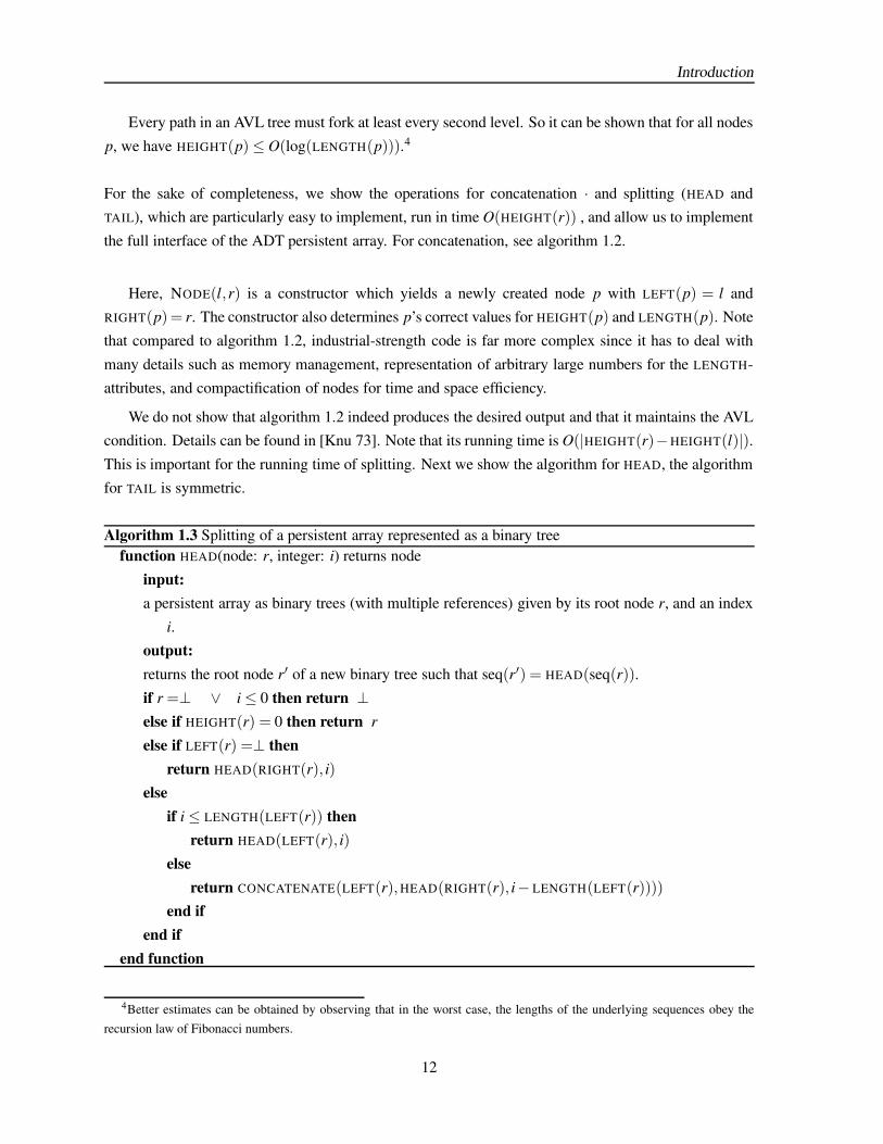
Every path in an AVL tree must fork at least every second level. So it can be shown that for all nodes
p, we have HEIGHT(p)≤ O(log(LENGTH(p))).4
For the sake of completeness, we show the operations for concatenation · and splitting (HEAD andTAIL), which are particularly easy to implement, run in time O(HEIGHT(r)) , and allow us to implement
the full interface of the ADT persistent array. For concatenation, see algorithm 1.2.
Here, NODE(l,r) is a constructor which yields a newly created node p with LEFT(p) = l andRIGHT(p) = r. The constructor also determines p’s correct values for HEIGHT(p) and LENGTH(p). Note
that compared to algorithm 1.2, industrial-strength code is far more complex since it has to deal with
many details such as memory management, representation of arbitrary large numbers for the LENGTH-attributes, and compactification of nodes for time and space efficiency.
We do not show that algorithm 1.2 indeed produces the desired output and that it maintains the AVLcondition. Details can be found in [Knu 73]. Note that its running time is O(|HEIGHT(r)−HEIGHT(l)|).
This is important for the running time of splitting. Next we show the algorithm for HEAD, the algorithmfor TAIL is symmetric.
Algorithm 1.3 Splitting of a persistent array represented as a binary treefunction HEAD(node: r, integer: i) returns node
input:a persistent array as binary trees (with multiple references) given by its root node r, and an index
i.output:returns the root node r′ of a new binary tree such that seq(r′) = HEAD(seq(r)).
if r =⊥ ∨ i≤ 0 then return ⊥else if HEIGHT(r) = 0 then return r
else if LEFT(r) =⊥ thenreturn HEAD(RIGHT(r), i)
elseif i≤ LENGTH(LEFT(r)) then
return HEAD(LEFT(r), i)
elsereturn CONCATENATE(LEFT(r),HEAD(RIGHT(r), i− LENGTH(LEFT(r))))
end ifend if
end function
4Better estimates can be obtained by observing that in the worst case, the lengths of the underlying sequences obey therecursion law of Fibonacci numbers.
12
1.4 The ADT Persistent Array
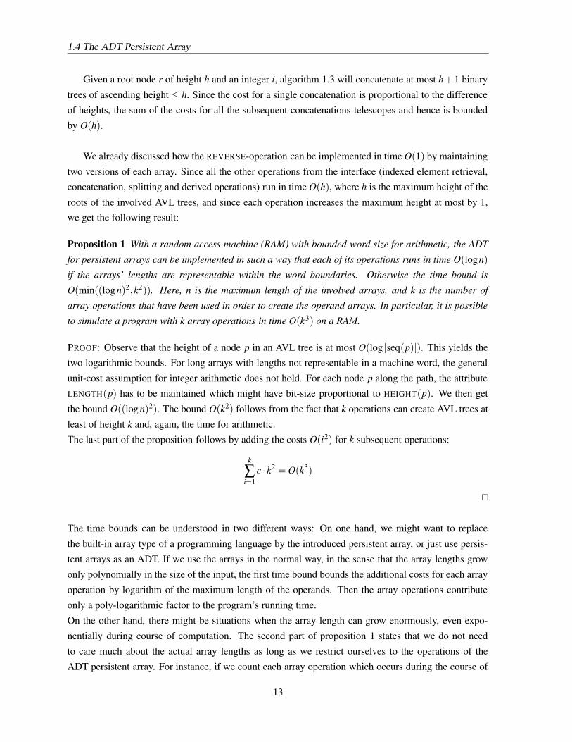
Given a root node r of height h and an integer i, algorithm 1.3 will concatenate at most h + 1 binary
trees of ascending height ≤ h. Since the cost for a single concatenation is proportional to the differenceof heights, the sum of the costs for all the subsequent concatenations telescopes and hence is bounded
by O(h).
We already discussed how the REVERSE-operation can be implemented in time O(1) by maintaining
two versions of each array. Since all the other operations from the interface (indexed element retrieval,concatenation, splitting and derived operations) run in time O(h), where h is the maximum height of the
roots of the involved AVL trees, and since each operation increases the maximum height at most by 1,we get the following result:
Proposition 1 With a random access machine (RAM) with bounded word size for arithmetic, the ADT
for persistent arrays can be implemented in such a way that each of its operations runs in time O(logn)
if the arrays’ lengths are representable within the word boundaries. Otherwise the time bound is
O(min((log n)2,k2)). Here, n is the maximum length of the involved arrays, and k is the number of
array operations that have been used in order to create the operand arrays. In particular, it is possible
to simulate a program with k array operations in time O(k3) on a RAM.
PROOF: Observe that the height of a node p in an AVL tree is at most O(log |seq(p)|). This yields thetwo logarithmic bounds. For long arrays with lengths not representable in a machine word, the general
unit-cost assumption for integer arithmetic does not hold. For each node p along the path, the attributeLENGTH(p) has to be maintained which might have bit-size proportional to HEIGHT(p). We then get
the bound O((log n)2). The bound O(k2) follows from the fact that k operations can create AVL trees at
least of height k and, again, the time for arithmetic.The last part of the proposition follows by adding the costs O(i2) for k subsequent operations:
k
∑i=1
c · k2 = O(k3)
2
The time bounds can be understood in two different ways: On one hand, we might want to replace
the built-in array type of a programming language by the introduced persistent array, or just use persis-
tent arrays as an ADT. If we use the arrays in the normal way, in the sense that the array lengths growonly polynomially in the size of the input, the first time bound bounds the additional costs for each array
operation by logarithm of the maximum length of the operands. Then the array operations contributeonly a poly-logarithmic factor to the program’s running time.
On the other hand, there might be situations when the array length can grow enormously, even expo-
nentially during course of computation. The second part of proposition 1 states that we do not needto care much about the actual array lengths as long as we restrict ourselves to the operations of the
ADT persistent array. For instance, if we count each array operation which occurs during the course of
13
Introduction
computation only once, the actual running time of our implementation will still only have an overhead
which depends polynomially — that is O(k3) — on the number k of array operations.
For some applications, it might be worthwhile to export some implementation-specific details suchas the LEFT and WRITE operations on inner nodes. This sometimes saves a logarithmic factor for certain
binary search schemes. We extend the ADT PERSISTENT ARRAY by the following operations:
1. LEFTPART(A): returns (non-deterministically) an array representing a prefix A’s sequence.
2. RIGHTPART(A): returns (non-deterministically) an arrays representing a suffix A’s sequence.
3. SOMEELEMENT(A): returns (non-deterministically) an element of the array A.
All three operations shall run in O(1) time. The operation SOMEELEMENT can easily be implemented
by storing additional information in the inner nodes of the binary tree.Note that for two arrays A and B, both representing the same sequence, the result of the operations above
is not necessarily the same. However, it always holds
A = LEFTPART(A) · RIGHTPART(A) .
Also we require for each array A of length n, that after O(log n) subsequent LEFTPART or RIGHTPART
operations (in any possible combination) the resulting array has length 0 or 1.
1.4.3 Homomorphisms on the Free Monoid
Assume we have an array of numbers, and we wish to maintain the sum over all its elements duringarray operations such as insertion, concatenation, splitting, etc. It would be very costly if, after each
operation, we had to iterate over all elements in order to recompute their sum. For instance, if x ∈ X ∗
with X =N is a finite sequence x = x0 . . .xn−1 of numbers xi ∈N, we would like to query segment sums:
that is, given two indizes i, j ∈ 0..n−1, we ask for the value
SEGMENTSUM(x, i, j) := h
(j
∑k=i
xk
).
If h is a function which maps any sequence y ∈ N∗ to the sum of all elements of y, then:
SEGMENTSUM(x, i, j) = TAIL(HEAD(x, j + 1), i)
Hence it would be nice if the images h(x) of a sequence x could be maintained under the operationsof the ADT PERSISTENT ARRAY . As it turns out, we can do this efficiently whenever h maps into
a set M which is equipped with an associative operation ·M and a neutral element eM , where in our
example M = N, ·M = +, and eM = 0. Such a structure M = (M, ·M,e) is called a monoid. The secondrequirement is that h is a homomorphism on the free monoid X ∗:
h(x · y) = h(x) ·M h(y), for all x,y ∈ X ∗
14
1.4 The ADT Persistent Array
Let X be a (possibly infinite) set of symbols, M = (M, ·,) be a monoid and h : X ∗→M be a homomor-
phism. Since X ∗ is the free monoid which is generated by X , h is uniquely definded by all the values h(x)
for x ∈ X . For strings v ∈ X ∗, many properties can be defined in terms of homomorphic images. Besides
of sums, another simple example are maxima: If X = R, the maximum of a sequence x0 · · ·xn−1, n≥ 0of real numbers is the image of x0 · · ·xn−1 under the homomorphism h :R∗→ (R∪−∞,max,−∞) which
is defined by h(x) = x for all x ∈R. In chapter 3 we will see other array parameters and transformations
that can be expressed this way.For computing the homomorphic image h(v) of a string v ∈ X ∗, it is sufficient to know only the restric-
tion of h on X , provided that we also know the multiplication and the neutral element of M. Thus whenwe say — in the context of a computer program — that a homomorphism h : X ∗ → M is given, we
actually mean that we are given a triple (h′, ·,e). Here the operation · is the multiplication of the monoid
M, e is its neutral element, and h′ is the restriction of h : X ∗→M to the set X of single elements.
As in our segment-sum example, sometimes a homomorphism h : X ∗→M is given in advance, and
we want to maintain the homomorphic image h(v) for all strings v ∈ X ∗ which occur during the courseof computation. In a binary tree representation B, we can achieve this by labelling each node p in B
with h(seq(p)). Therefore, we modify the constructor of inner nodes p in such a way that, besides
of LEFT(p) and RIGHT(p), the constructor also gets the multiplication · : M×M→M as a parameter.Then, by homomorphy:
h(seq(p)) = h(seq(LEFT(p))) ·h(seq(RIGHT(p)))
It follows:
Proposition 2 Let h : X ∗ → M be a fixed monoid homomorphism. By using AVL trees (with multiple
references), it is possible to maintain homomorphic images h(A) of all persistent arrays A in such a
way that the additional costs stem solely from computing h(x) for newly created array elements x ∈ X
and from multiplications in M for the inner nodes. The latter is bounded by O(min(logn,k)) for each
single operation, where n is the maximum length of the involved arrays, and k is the number of array
operations that have been used in order to create operands. In particular, it is possible to simulate k
steps of a random access machine — equipped with array operations on the ADT PERSISTENT ARRAY
— in time O(k3) plus the time needed for O(k2) multiplications in M.
The proposition is similar to proposition 1 and additionally states that maintaining homomorphic imagesfor a fixed homomorphism h does not do any harm as long as the costs for mapping of single elements
and for multiplication in the range of h can be neglected. Note that this proposition extends easily toany constant number of homomorphisms.
Sometimes we do not want to maintain images under previously fixed homomorphisms. What wewant is to compute an array’s A image h(A) for a given homomorphism h. This can be accomplished by
traversing the binary tree which represents A:
15

Introduction
Proposition 3 Let h : X ∗→M be a fixed monoid homomorphism. For a particular persistent array A
which occurs in the kth step of a computation, it is possible to compute its homomorphic image in such
a way that the costs stem solely from multiplications in M and from computing h(x) for the leaf elements
of the AVL tree (with multiple references) which represents A. The number of multiplications is bounded
by the number of inner nodes of the tree, which is O(min(k2, |A|).
Note that while homomorphisms are useful, their usage is — compared to the standard operations onpersistent arrays — somewhat restricted: Either we maintain images for a fixed finite set of homo-
morphism during the course of computation, or we halt the computation and compute homomorphicimages afterwards. The propositions above give reasonable bounds on the number of operations. Note,
however, that it is inherently more difficult to derive appropriate time bounds if the computation of
homomorphism is interwoven with the usual array operations from the ADT. For instance, for a given n
A := [1]
let h : 0,1∗→0,1∗ be the homomorphism defined by h(0) = 0, h(1) = 11
for i = 0..n−1 doA := h(A)
end for
runs in time polynomial in n only when we assume appropriate copy semantics in the computation ofh(x). If each time the array which represents h(x) is newly created, then the running time can actually
be exponential in n.
On the other hand, the same resulting string will be computed by
A := [1]
for i = 0..n−1 doA := A ·A
end for
always in time polynomial in n.
1.4.4 Impossibility of Pairing
Given two strings v = x1 · · ·xn, w = y1 · · ·yn, both of length n, we would like to construct a persistent
array C for the string v×w := (x1,y1) · · · (xn,yn) ∈ (X ×X)∗. The operation which maps v,w to v×w
is called pairing. A representation of the string v×w in form of a persistent array C would permit to
build many other operations on top of it: For instance, if v,w are two n-vectors of natural numbers, we
could use a homomorphism which maps v×w to the n-vector of element-wise sums. This would allowvector addition even for vectors of exponential length — as long as the persistent array representation is
of polynomial size. Another example is to use C in order to decide if v,w are equal: All we have to do
16
1.4 The ADT Persistent Array
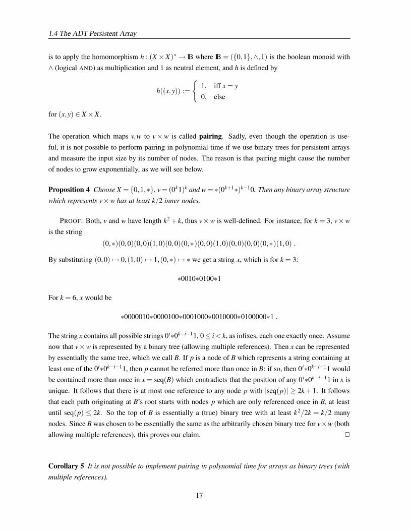
is to apply the homomorphism h : (X ×X)∗→ IB where IB = (0,1,∧,1) is the boolean monoid with
∧ (logical AND) as multiplication and 1 as neutral element, and h is defined by
h((x,y)) :=
1, iff x = y
0, else
for (x,y) ∈ X×X .
The operation which maps v,w to v×w is called pairing. Sadly, even though the operation is use-
ful, it is not possible to perform pairing in polynomial time if we use binary trees for persistent arraysand measure the input size by its number of nodes. The reason is that pairing might cause the number
of nodes to grow exponentially, as we will see below.
Proposition 4 Choose X = 0,1,∗, v = (0k1)k and w = ∗(0k+1∗)k−10. Then any binary array structure
which represents v×w has at least k/2 inner nodes.
PROOF: Both, v and w have length k2 + k, thus v×w is well-defined. For instance, for k = 3, v×w
is the string
(0,∗)(0,0)(0,0)(1,0)(0,0)(0,∗)(0,0)(1,0)(0,0)(0,0)(0,∗)(1,0) .
By substituting (0,0) 7→ 0,(1,0) 7→ 1,(0,∗) 7→ ∗ we get a string x, which is for k = 3:
∗0010∗0100∗1
For k = 6, x would be
∗0000010∗0000100∗0001000∗0010000∗0100000∗1 .
The string x contains all possible strings 0i∗0k−i−11, 0≤ i< k, as infixes, each one exactly once. Assumenow that v×w is represented by a binary tree (allowing multiple references). Then x can be represented
by essentially the same tree, which we call B. If p is a node of B which represents a string containing at
least one of the 0i∗0k−i−11, then p cannot be referred more than once in B: if so, then 0i∗0k−i−11 wouldbe contained more than once in x = seq(B) which contradicts that the position of any 0 i∗0k−i−11 in x is
unique. It follows that there is at most one reference to any node p with |seq(p)| ≥ 2k + 1. It follows
that each path originating at B’s root starts with nodes p which are only referenced once in B, at leastuntil seq(p) ≤ 2k. So the top of B is essentially a (true) binary tree with at least k2/2k = k/2 many
nodes. Since B was chosen to be essentially the same as the arbitrarily chosen binary tree for v×w (bothallowing multiple references), this proves our claim. 2
Corollary 5 It is not possible to implement pairing in polynomial time for arrays as binary trees (with
multiple references).
17

Introduction
PROOF: Set k = 2n. By fast exponentiation, persistent arrays (as binary trees with multiple refer-
ences) for the strings v,w from proposition 4 can be constructed in time polynomial in n and thus haveonly a polynomial number of nodes. By proposition 4 any representation of v×w as a binary tree has at
least Ω(2n) many nodes and thus cannot be constructed from the binary trees (with multiple references)for v and w in polynomial time. 2
But would other implementations of the ADT PERSISTENT ARRAY be of any benefit? That is, canwe still simulate a machine equipped with array concatenation and pairing in polynomial time in such
a way that afterwards we can compute homomorphic images efficiently? The answer is negative in thefollowing sense:
Corollary 6 For k = 2n, the arrays v,w in the proof of proposition 4 can be constructed by a program
equipped with array concatenation with a polynomial (in n) number of steps. However:
1. It is impossible to represent v×w in such a way that there is a generic algorithm which, for any monoid
homomorphism h : (X×X)∗→M, computes h(v×w) by a polynomial number of multiplications, start-
ing from the images h(X)⊆M.
2. Let h : (X ×X)∗ → M be a homomorphism such that any element of M generated by h(X) ⊆ M, and
a program which uses a polynomial number of multiplications (in M), can be also be computed in
polynomial time. Then h can be chosen in such a way that h(v×w) cannot be computed in polynomial
time.5
PROOF: The proof is clear by choosing h to be the identity map on (X ×X)∗, and representing the
images of h as binary trees with multiple references. (More formally, h is a homomorphism betweentwo different representations of (X × X)∗, where structures representing the same string are identi-
fied). Firstly, any generic algorithm which computes h(v×w) as shown in the first part of the corollary
must fail by proposition 4. Secondly, observe that h fulfills the requirements of the second part of thecorollary by proposition 1. Hence polynomial-time construction of h(v×w) contradicts proposition 4. 2
Thus pairing cannot be a polynomial time operation for any polynomial-time implementation of the
ADT PERSISTENT ARRAY which allows efficient computation of homomorphic images. The results
suggest that it is better to exclude pairing from the interface of persistent arrays. It also indicates thatdeciding equality (in terms of the sequence of elements) of persistent arrays represented as binary trees
A,B is difficult when multiple references are involved (thus that the lengths can grow exponentially).However, in section 3.1.1 we will give a partial solution by describing a probabilistic equality test.
By using the same construction as in proposition 4 we get:
5Note that the time for computing (x,y) 7→ h((x,y)) for single pairs (x,y) ∈ X ×X can be ignored since the number ofelements of X = 0,1,∗ is finite.
18

1.5 Related Work
Corollary 7 For each n≥ 0, there exist strings v,w ∈ 0,1∗ whose representation as binary trees with
multiple references is constructable in time polynomial in n, such that each binary tree representing the
sum of v and w (interpreted as binary numbers) needs an exponential number of nodes.
1.5 Related Work
Dynamic arrays with concatenation and splitting and their implementation as balanced trees are well-known. They can be found in many textbooks on algorithms and data structures, see [Knu 73] for an
implementation as AVL trees, or [CLRS 01] for an implementation as red-black trees. In [Knu 73],
Knuth credits C.A. Crane’s 1972 thesis for the first description of concatenating and splitting AVL trees.In the literature for functional data structures and also for graph algorithms, fully persistent arrays belong
to the fundamental data structures for a long time. The possibility of maintaining homomorphic images
is a fact which is rarely explicitely mentioned. Still we believe that our explicit treatment is worthwhile,since the homomorphism technique can be considered as a programming interface which generalizes
from many data structures. As an example see the J. Burghardts’s paper [Bur 02] about segment sumqueries. String homomorphisms have also been studied as a tool for parallelizing algorithms. Our
explicit upper bounds for polynomial time simulation of persistent arrays in connection with proposition
4 about the impossibility of pairing are new in this thesis.
19


Chapter 2
Graph Algorithms and Persistent Arrays
In the first chapter we described the basic properties of persistent arrays. In particular we stressed thattheir representation allows sharing of subarrays. Furthermore, we stated that persistence makes the
design of algorithms easier. The purpose of this chapter is to justify this claim in the context of graphalgorithms.
The main idea behind the data structures and algorithms in this chapter is to represent paths as per-sistent arrays. Persistent arrays provide an interface for obtaining other information on a given path by
means of homomorphic images, which might be useful as a general interface in programming libraries.
We have already seen in section 1.4.3 how homomorphic images can be maintained efficiently for per-sistent arrays. For example, assume that a train route is represented as a string v = s0d1s1 . . . sn−1dnsn,
where each si is a station and di is the distance from si−1 to si. Then the following information can beobtained in terms of homomorphisms:
1. The total distance ∑ni=1 di.
2. The maximum distance max(d0, . . . ,dn) in between two stations.
3. A string si(0)si(1) . . . si(k), 0 ≤ i(0) < i(1) < .. . < i(k) ≤ n containing only particular stations, forinstance stations where the train halts or stations with special facilities for maintenance etc.
In this chapter, we will see how paths, represented as persistent arrays, can be maintained within several
known graph algorithms and data structures:The first section deals with dynamic tree algorithms. Dynamic data structures for (undirected) trees are
fundamental for many dynamic graph algorithms, for instance for solving dynamic connectivity prob-lems. We will use Henzinger and King’s ET trees as a data structure for dynamic trees (see [HLT 01]).
ET trees are easy to implement but do not maintain path information or global tree parameters such as
center. We will show how persistent arrays can be used in order to maintain path information and centerunder update operations while retaining the simplicity of the data structure. Our resulting data structure
has not the asymptotically best performance, but is easy to implement and updates and queries still run
21

Graph Algorithms and Persistent Arrays
in poly-logarithmic time.
In the concluding sections of this chapter we will prepare the semiring framework for using per-
sistent arrays for all-pairs-shortest-path (APSP) algorithms. We also show how the successor matrix
representation of a solution of the APSP problem can be efficiently transformed into a matrix of persis-tent arrays.
2.1 Paths in Dynamic Trees and Forests
First, we settle some notation: Let G = (N,E) be an undirected graph. G is a forest if G is acyclic (but
not necessarily connected). If G is a forest and connected, then we call G a tree.Throughout the entire section, a path π is a finite sequence π = a0 . . .ak of nodes ai ∈ N, such that for
0 ≤ i < k the nodes ai,ai+1 are adjacent to each other. We write src(π) for a0 and dst(π) for ak . The
length of a path π is its number k of traversed edges. Our algorithms represent paths as persistent arrays,thus making it possible to join two given paths π,π ′ in logarithmic time (depending on their length).
Also, we can retrieve the ith node of a path in logarithmic time. Note that joining π and π ′ only yields apath if dst(π) = src(π ′), and that we actually remove either dst(π) or src(π ′) before concatenation. The
notation π : p→G q means that π is a path (in the underlying graph G) with src(π) = p, dst(π) = q. The
subscript G will be usually omitted.
From now, let T = (N,E) be a tree. For each pair of nodes p,q ∈ N there exists a unique simple
path π : p→ q, denoted by π(p,q) := π . The main idea of this section is to compose simple paths in
order to gain another simple path:
Proposition 8 Let p,q,r ∈ N and let a0 . . .ak = π(r, p), b0 . . .bm = π(r,q). Then there exists no pair of
indices i < j ∈ 0 . . .min(k,m) such that ai 6= bi and a j = b j .
PROOF: Asume such a pair i < j exists. Since a0 = b0 = r there exists a maximum s < i with πs = π ′s.Because of π0 = π ′0 = r there exists a minimum t > i with πt = π ′t . Thus, the path as,as+1, . . . ,at con-
nected with bt ,bt−1, . . . ,bs forms a cycle, which contradicts that T is a tree. 2
From proposition 8 we see that for a0 . . .ak = π(r, p) and b0 . . .bm = π(r,q), the maximum index s
with as = bs is well-defined. It divides the paths π(r, p),π(r,q) into a common subpath and two node-
disjoint subpaths which then form the (unique) simple path π(p,q):
Corollary 9 Let be p,q ∈ N and a0 . . .ak = π(r, p), ai ∈ N, 0 ≤ i ≤ k and b0 . . .bm = π(r,q), bi ∈ N,
0≤ i≤ m. Choose s = 0 . . .min(k,m) such that a0 . . .as = b0 . . .bs is the longest common prefix of both
paths. Then π(p,q) = akak−1 . . .asbs+1bs+2 . . .bm.
22

2.1 Paths in Dynamic Trees and Forests
The proof is immediate by observing that akak−1 . . .as and bsbs+1 . . .bm have only the node as = bs in
common. This node as = bs from above is denoted by MEET(p,q,r), it is the intersection of the threepaths connecting p,q,r.
Now, for two simple paths π = π(r, p), π ′ := π(r,q) with k and m nodes respectively, we can compute
MEET(p,q,r) in O((logmin(k,m))2) + O(logmax(k,m)) time. Within the same time bounds, we cancompose π(r, p) and π(r,q) in such a way that we gain the (unique) simple path π(p,q). The resulting
algorithm is algorithm 2.1 for composing two simple paths to another simple path, which implicitly
computes MEET(p,q,r).
Algorithm 2.1 Path Compositionfunction COMPOSESIMPLEPATHS(π ,π ′ )
Input: two simple paths π : r→ p, π ′ : r→ q, represented as persistent arraysOutput: the simple path π(p,q)
k := min(LENGTH(π),LENGTH(π ′ ))i := 0; j := k−1
π := HEAD(π,k)
π ′ := HEAD(π ′,k)
while i 6= j dos := d( j− i)/2eif π[s] = π ′[s] then
i := s
elsej := s−1
end ifend while(π[i] = π ′[i] is now MEET(p,q,r))
return REVERSE(TAIL(π , i))·TAIL(π ′ , i + 1)end function
In order to achieve the time bounds, observe that the binary search in the first part of algorithm 2.1
accesses the arrays O(log min(k,m)) times, while each access needs O(logmin(k,m)) time. Hence thefirst term O((logmin(k,m))2). Finally, splitting and concatenation need O(logmax(k,m)) time each.
2.1.1 Path Queries on Static Trees
Before we turn to the dynamic case, we will consider path queries on a given static tree T = (N,E) withn nodes. The goal of a path query PATH(p,q) is, given two nodes p,q, to yield the simple path π(p,q).
A direct consequence of the path-composition algoritm 2.1 is:
23

Graph Algorithms and Persistent Arrays
Proposition 10 Given a fixed r ∈ N and a table of all π(r, p), p ∈ N, represented as persistent arrays.
Then for any pair of nodes p,q ∈ N, a persisent array representing π(p,q) can be constructed in time
O((logm)2), where m is the length of the longest simple path in T .
For most “natural" graph representation of a tree T = (N,E) and any given r ∈ N, such a tableπ(r, p), p ∈ N can be constructed efficiently by using DFS traversal. For instance, a natural represen-
tation of a tree T is by a collection of adjacency lists, which for each node store the list of adjacent
nodes. This representation needs — since T is a tree — Θ(n) space. Adjacency lists do not support pathqueries, but they permit traversal of the nodes N depth-first (DFS-order) in O(n) time, starting from
r ∈ N.
Algorithm 2.2 Construct Table of Paths rooted in rfunction CONSTRUCTTABLE(graph G, node r)
input:An undirected tree G = (N,V ) and a arbitrary root node r ∈ N. It is assumed that G is represented
in a natural way which supports DFS-traversal without additional overhead
result:constructs the table path[] with path[p] = π(r, p)
〈 mark all nodes p ∈ N as unvisited 〉VISIT(r,ε ,0)
end functionfunction VISIT(node p, Array P) returns number of visited nodes
if 〈 p is not already visited〉 then〈 mark p as visited〉P := CONCATENATE(P,[q])
path[p] := P
for 〈 all nodes q adjacent to p 〉 doVISIT(q,P)
end forend if
end function
By using DFS traversal we can now transform T ’s representation (as adjacency lists) into the tableπ(r, p) by bookkeeping the simple path from r to the currently visited node p. By proposition 10, the
resulting table π(r, p) permits path queries in O((logn)2) time. Algorithm 2.2 will construct π(r, p) for
all p ∈N simultaneously in time O(n log n), where the additional logarithmic factor stems from the timefor concatenating persistent arrays. Note that the space requirements for representing the table π(r, p)
in memory is naturally bounded by the running time of algorithm 2.2, which is O(n logn).
24

2.1 Paths in Dynamic Trees and Forests
As we see, a representation of a tree T (which allows DFS traversal without additional overhead
except the time for visiting the nodes), can be transformed into a representation such that:
1. The new representation needs O(n logn) space.
2. Path queries and MEET-queries need time O((logm)2), where m ≤ n is the length of the longestsimple path in T .
3. The transformation needs O(n log n) time.
2.1.2 Path Queries on Dynamic Trees
A dynamic forest is a data structure which represents a collection of dynamic trees, allowing updates on
the set of edges. The two most important update operations are linking two formerly disconnected treesby a newly introduced edge, and splitting a tree by removing one of its edges.
An interesting application for trees and forests as dynamic data structures are computer networks – theirtopologies are often trees themselves. Other applications of dynamic forests arise in dynamic graph
algorithms, such as maintaining spanning trees for connected components or for solving several con-
nectivity problems (see [HLT 01]).
Many data structures have been proposed for dynamic trees, among them Heinzinger and King’s ETtours, which are particularly simple to implement. More elaborate data structures rely on a recursive
decomposition of trees and are far more complicated to implement than ET trees (for instance topol-
ogy tree [Fre 85] and top trees [AHLT 03]). While topology trees and top trees are very efficient andversatile, nevertheless ET trees suffice for many porposes. In their standard version, all three data struc-
tures allow updates in O(logn) time, but only top trees and topology trees maintain path informationand global graph parameters such as diameter. In the remainder of this section we want to fill the gap
between the highly efficient and versatile data structures for dynamic trees and the much easier to imple-
ment ET trees: We will show how ET trees can be modified in such a ways that they allow to maintainpaths and diameters. Additional path parameters like maximum edge-value ot total distance can then be
maintained in terms of homomorphic images (see section 1.4.3). The resulting data structure retains the
simplicity of ET trees, and still implements trees with updates and queries in poly-logarithmic time.The running time per update and path query will be O(logn(log m)2), where n is the size of the tree(s),
measured in the number of nodes, and m is the maximum number of nodes for a simple path in theforest. For updates, this is by a factor (log m)2 worse than the best known data structures; for path
queries (when paths are represented as persistent trees) it is worse by a factor of log m. Our interest in
using ET trees is legitimated since they permit simple implementations for prototyping or for building atest bench for the more elaborated data structures.
Let F = (N,E) be a forest consisting of the maximal trees (in the meaning of not being proper
subtrees included within other trees in F) T1, . . . ,Tk. Deleting any edge from F will increase the number
25

Graph Algorithms and Persistent Arrays
of maximal trees by one. For disconnected p,q∈N, adding the edge (p,q) will yield another forest F ′=
(N,E∪(p,q)) with the number of maximal trees reduced by one. We have the following fundamentalupdate operations:
1. LINK(p,q): Given two disconnected nodes p,q ∈ N, returns the forest F ′ = (N,E ∪(p,q)).
2. UNLINK(p,q): Given two adjacent nodes p,q ∈ N, returns the forest F ′ = (N,E \(p,q))
Next to update operations, we want to support the following queries:
1. ISCONNECTED(p,q): Given two nodes p,q ∈ N, determines whether they are connected.
2. PATH(p,q): Given two connected nodes p,q ∈ N, returns the simple path π(p,q).
3. ISBETWEEN(p,q,r): Given three connected nodes p,q,r ∈ N, determines whether r lies on thesimple path π(p,q).
4. MEET(p,q,r): Given three connected nodes p,q,r ∈ N, returns the (unique) intersection point ofthe three paths between each pair of the nodes p,q,r.
5. CENTER(p): Given a node p ∈ N, returns a center of Ti, where Ti is the maximal tree which
contains p.
6. DIAMPATH(p): Given a node p ∈ N, returns a simple path of maximum length in Ti, where Ti is
the maximal tree which contains p.
7. DIAM(p): Given a node p ∈ N, returns a diameter path of Ti, where Ti is the maximal tree whichcontains p.
For the definition of diameter, diameter path, and center see section 2.1.3.
MEET and ISBETWEEN can be implemented in terms of path queries: For computing MEET wecan use path composition, while for ISBETWEEN(p,q,r), we find that r lies on π(p,q) if and only if
MEET(p,q,r) = r.
In order to allow update operations and the remaining queries, we linearize a tree by transforming itto one of its Euler tours, which in turn is represented as a so-called ET tree: In a directed graph, an
Euler tour is a closed path which traverses every edge exactly once. An Euler tour of an undirected treeT is then an Euler tour of its directed equivalent T ′ = (N,(p,q) : p,q ∈ T). There always exists
at least one Euler tour, since in T ′ all nodes have the same in-degree and out-degree. For a pictorial
representation of a tree’s Euler tour see figure 2.1.
Proposition 11 Let T = (N,E) be a non-empty tree. The set of Euler tours for a tree T can be defined
recursively as the smallest set fulfilling the following properties:
(i) If T = (p, /0), then the path π = pp is the only Euler tour in T .
26

2.1 Paths in Dynamic Trees and Forests
01
2
3
4
5
6
7 8
9
Figure 2.1: An Euler tour around a undirected tree
(ii) Let be T = (N1∪N2,E1∪E2∪p,q) such that Ti = (Ni,Ei), i = 1,2 are trees and N1∩N2 = /0,p ∈ N1, q ∈ N2. Let be s1 ∈ N1 and let π1 : s1→ p, π ′1 : p→ s1 be paths in T1 such that π1π ′1 is an
Euler tour in T1. Similarly, let be s2 ∈ N2 and let π2 : s2→ q, π ′2 : q→ s2 be paths in T2 such thatπ2 ·π ′2 is an Euler tour in T2. Then π1 · (p,q) ·π ′2 ·π2 · (q, p) ·π ′1 is an Euler tour of T .
The operation · joins two paths π0, . . . ,πm and π ′0, . . . ,π ′k with πm = π ′0 to π0, . . . ,πm−1,π ′0, . . .π ′k. Propo-
sition 11 yields an equivalent definition of Euler tours in terms of a recursive decomposition of trees.We can represent each maximal tree Ti = (Ni,Ei) of the forest F by the sequence of directed edges of
some (arbitrarily chosen) Euler tour of Ti. If now we store the Euler tours in AVL trees, in a similar
way as we implemented persistent arrays, we can split and concatenate Euler tours in logarithmic time.Since an Euler tour traverses each directed edge exactly once, the AVL tree has no multiple references
to any of its inner nodes. This allows us to maintain uplinks from each inner node (except the root
node) to its unique successor. The resulting structure is called an ET tree. In ET trees we can set theuplinks in the constructor calls of algorithms 1.2 and 1.3. Note that since this modification causes the
constructor to operate destructively on its children, ET trees are not persistent.A forest F = (N,E) is now represented by a collection of ET trees ETi, one for each of F’s maximal
trees Ti = (Ni,Ei). In addition to the ET trees, we will maintain a dictionary which, for each directed
edge (p,q) with p,q ∈E , allows us to find the corresponding leaf node in F’s collection of Euler trees.The dictionary is organized in such way that, given a node p ∈ N, it returns an arbitrary directed edge
(p,q) with p,q ∈N or⊥ if no such edge exists. Also, given a directed edge (p,q) with p,q ∈Ni thedictionary returns the leaf labeled with (p,q) of the corresponding ET tree ETi. As an example, let us
consider figure 2.2: We want to test whether or not the points p = 5 and q = B are connected. Assume
that for the nodes 5 and B the dictionary returns the edges (5,9) and (B,A), respectively. The uplinksfrom edge (5,9) will allow us to walk upward in ET1 via the nodes e16,e9,e4,e2,e1. At the same time,
the uplinks from edge (B,A) will allow us to walk upward in ET2 via the nodes e22,e21. Since e1 and
27

Graph Algorithms and Persistent Arrays
0
2
3
6
F:T11
4
5
7 8
9
T2
E
A
B C
D
6336
34 45 59 95
87
57 78 75 54 43 32 21 12
20 02
23 DA AB
BA
AC CA AD
DE ED
ET
ET1
2
e
e
e
e
e
e
e e e
e
e
e
e
e
e
e
1
2 3
5 6 7
8 910 11 12 13
15 1617e
21
2223
24 25 26
27 28
e e
e
4e
e
e
e14 e
Figure 2.2: A forest F consisting of two maximal trees T1, T2 and two corresponding ET trees
e21 are the roots of two distinct ET trees, p and q are disconnected in F .
After having discovered that p and q are disconnected, we want to join both trees by introducing
the edge p,q to the forest F . Again, we find two corresponding paths to the root nodes of their
respective ET trees, but this time we memorize the positions of the leaf nodes from where we started.This allows us to use the splitting operation HEAD and TAIL in order cut the Euler tour at appropriate
positions for p ∈ T1 and q ∈ T2 and then to concatenate the results in order to obtain an ET tree for the
tree T = (N1∪N2,E1∪E2∪p,q).
Indeed, proposition 11 shows us how to maintain Euler trees during updates through concatenatingand splitting. Also, by using the uplinks in the ET trees, we can determine in logarithmic time whether
any two nodes are connected.
For an inner node e of an ET tree ETi, the edges which are contained in the leaves of the subtree
at e form a (not necessarily simple) path in forest’s corresponding tree Ti. We call this path the Eulersubtour at e, denoted by st(e). In order to allow path queries, we maintain for each e the simple path
π(src(st(e)),dst(st(e))), represented as a persistent array.
Let e be the inner node of an ET tree ETi. If e is a leaf, then st(e) consists solely of the directed edge(p,q) which e contains, and π(src(st(e)),dst(st(e))) = st(e) = pq. If e is an inner node of ETi with
only one child e′, then st(e) = st(e′) and we get π(src(st(e)),dst(st(e))) = π(src(st(e′)),dst(st(e′))).
28

2.1 Paths in Dynamic Trees and Forests
Finally, we have the case that e1,e2 are the left and the right children of e. Then src(st(e)) = src(st(e1)),
dst(st(e)) = dst(st(e1)) and dst(st(e1)) = src(st(e2)). Hence we can compute π(src(st(e)),dst(st(e)))
by composing π(src(st(e1)),dst(st(e1))) and π(src(st(e2)),dst(st(e2))). Using algorithm 2.1, this needs
O(logm) time per inner node e, where m is the maximum number of edges of any simple path. Hence,each update operation takes O(logn(log m)2)≤ O((logn)3) time.
Let p,q ∈ N be connected. In order to extract the simple path π(p,q), we first find the corresponding
ET tree ETi together with appropriate positions of p,q within the Euler tour. By splitting and concate-nating ETi appropriately, we obtain an ET tree ET ′ with root node r such that π(src(st(r)),dst(st(r))) =
π(p,q)1.
2.1.3 Diameter, Center, and Diameter Path
For p,q ∈ N, dist(p,q) is the distance (either the number of edges or the sum of positive edge weights)
of the simple path from p to q.
Definition 4 Let G = (N,E) be a connected graph. A simple path π : p,q of maximal total distance
dist(p,q) is called a diameter path, and |π| the diameter of G. A node p which minimizes
maxq∈N
dist(p,q)
is called a center of G.
Observation 12 Let T = (N,E) be a tree and let π : m1 → m2, m1,m2 ∈ N be a diameter path in T .
Then:
(i) Let p ∈ N such that π traverses p. Then there exists no q ∈ N \ π such that dist(p,q) >
min(dist(p,m1),dist(p,m2)).
(ii) π traverses at least one of T ’s centers.
(iii) For all p ∈ N, at least one of the nodes m1 or m2 has maximal distance to p.
PROOF: (i) Assume there exists q ∈ N \π with dist(p,q) > min(dist(p,m1),dist(p,m2)). Without loss
of generality assume further that dist(p,m1)≥ dist(p,m2). Since the simple paths π(m1, p) and π(p,q)
have no edge in common, we get
dist(m1,q) = dist(m1, p) + dist(q, p) > |π| ,
which contradicts that π is a diameter path.
(ii) follows directly from (i)
(iii) For p,q ∈ N, choose i 6= j ∈ 1,2 such that the diameter path from mi to m j traversesMEET(m1,m2, p) not before it traverses MEET(m1,m2,q). Without loss of generality we assume i = 1.
1Since the operations HEAD and TAIL destroy the uplinks of the original ET tree ETi, we have to replace ETi by ET ′.
29
Graph Algorithms and Persistent Arrays
Further, assume dist(q, p) > dist(m1, p). It follows dist(q,r) > dist(m1,r) for each node r ∈ N which is
traversed by the simple path π(m1, p), especially for r := MEET(m1,m2, p). The choice of i ensures thatthe simple paths π(q,r) and π(r,m2) are edge-disjoint, hence
dist(q,m2) = dist(q,r) + dist(r,m2)> dist(m1,r) + dist(r,m2) = |π| ,
which contradicts that π is a diameter path. 2
Again, let e be the inner node of some ET tree ETi and st(e) be the Euler subtour at e. The nodeswhich are traversed by st(e) induce a tree T (e) in the forest F , more specifically a subtree of the tree Ti
which is represented by ETi. The main idea is to maintain, for each such e, a diameter path for T (e).Again, we represent diameter paths as persistent arrays. With slight modifications, i.e. storing the edge
weights inbetween two adjacent nodes and using an appropriate homomorphism, we can maintain the
total cost of each path, which in case of a diameter path yields the diameter of the tree. Furthermore, wecan extract tree centers by using a binary search, which needs time O((log |π|)2) in a persistent array
which represents the diameter path π .
The task of maintaining diameter paths in ET trees is complicated by the fact that, for two innernodes e,e′ within the same ET tree, the trees T (e), T (e′) are not necessarily disjoint. But the following
propositions show that this does no harm:
Observation 13 Let Ti = (Ni,Ei), i = 1,2 be two (not necessarily edge-disjoint) trees such that T ′ =
(N1∪N2,E1∪E2) is also a tree. Then:
(i) (N1∩N2,E1∩E2) is a tree.
(ii) A simple path π in T ′ lies either completely in T1 or completely in T2, or there exist p ∈ N1 \N2
and q ∈ N2 \N1 such that π : p→ q or π : q→ p.
The proof is obvious by using the cycle-freeness property of (N1∪N2,E1∪E2).
Proposition 14 Let Ti = (Ni,Ei), i = 1,2 be two (not necessarily edge-disjoint) trees such that T ′ =
(N1∪N2,E1∪E2) is also a tree. Furthermore, choose m1,m2 ∈ N1, m3,m4 ∈ N2 such that dist(m1,m2)
is maximal in T1 and dist(m3,m4) is maximal in T2. Then the diameter of T ′ is
maxp,q∈N1∪N2
dist(p,q) = max( dist(m1,m2),dist(m1,m3),dist(m1,m4),
dist(m2,m3),dist(m2,m4),dist(m3,m4)) .
PROOF: Let p,q be two nodes of maximal distance in the tree T ′ and π : p = π1, . . . ,πn = q be a corre-
sponding diameter path. If π lies entirely in T1 or entirely in T2 then the diameter of T ′ is dist(m1,m2)
or dist(m3,m4). Otherwise assume without loss of generality that p ∈ N1 \N2 and q ∈ N2 \N1. Let k be
the largest index such that π1,π2, . . . ,πk lies entirely in T1. According observation 12 (iii), m1 or m2 has
30

2.2 The Semiring Framework for Shortest Paths
maximal distance to r. Hence, in π we can replace π1,π2, . . . ,πk by the simple path π(mi,πk) for appro-
priate i ∈ 1,2. Analogously, we can replace π j, . . . ,πn by the simple path π(π j,mi) for appropriatei ∈ 3,4, where j is the smallest index such that π j, . . . ,πn lies entirely in T2. 2
Given an ET tree ETi for the tree Ti = (Ni,Ei), we store the following information in each inner node
e of ETi:
• s(e) = src(st(e)) and t(e) = dst(st(e)), i.e. the nodes where e’s corresponding Euler subtour starts
and ends.
• m1(e) and m2(e), which are two nodes of maximal distance in e’s corresponding subtree of T (e)⊆Ti (i.e. the tree consisting of all edges which are traversed by e’s Euler subtour).
• The following simple paths: π(s(e), t(e)), π(m1(e),m2(e)), π(s(e),m1(e)), π(s(e),m2(e)),
π(m1(e), t(e)), and π(m2(e), t(e)).
Note that π(s(e), t(e)) has already been used in order to maintain simple paths. The other five paths
can be used in order to maintain diameter paths recursively for each inner node e of ETi, sinceπ(m1(e),m2(e)) is a diameter path of e’s corresponding subtree of T (e):
If e is a leaf node it is clear how to compute the required information. If e has only one child
e′, then we we take the information from e′. Now assume e,e1,e2 are three inner nodes of ETi
such that e1,e2 are, respectively, the left and the right child of e. Forthermore, assume we already
know s(e1,2), t(e1,2), π(s(e1,2), t(e1,2)), π(m1(e1,2),m2(e1,2)), π(s(e1,2),m1(e1,2)), π(s(e1,2),m2(e1,2)),π(m1(e1,2), t(e1,2)), and π(m2(e1,2), t(e1,2)). By path composition we can compute the simple paths
π(s(e), t(e)), π(m1(e1),m1(e2)), π(m1(e1),m2(e2)), π(m2(e1),m1(e2)), and π(m2(e1),m2(e2)). By
maintaining the total distance of each path, we can use observation 14 in order to choose two nodesm1(e),m2(e) ∈ m1(e1),m2(e1),m1(e2),m2(e2) of maximal distance in T (e). Again, by composi-
tion of the appropriate paths, we compute the paths π(m1(e),m2(e)), π(s(e),m1(e)), π(s(e),m2(e)),
π(m1(e), t(e)), and π(m2(e), t(e)). The number of compositions is constant, hence for each node e ofETi we need O((log m)2) time, where m≤ n is the maximal number of nodes of any simple path in Ti.
Corollary 15 In a dynamic forest F, we can, for each maximal tree Ti, maintain diameter, center, and a
diameter path in O(logn(log m)2) time per update, where m≤ n is the maximal number of nodes for a
simple path in F.
2.2 The Semiring Framework for Shortest Paths
Shortest-paths and shortest-distance problems on general graphs are often generalized in such a waythat they work on semirings. The concept of a semiring abstracts of the operations of adding costs and
obtaining minima:
Definition 5 A semiring is a structure R = (R,+R,×R,0R,1R) such that
31
Graph Algorithms and Persistent Arrays
(i) (R,+R,0R) is a commutative monoid,
(ii) (R,×R,1R) is a monoid,
(iii) ×R distributes over +R, that is, for a,b,c ∈ R the laws of distributivity hold:
(a +R b)×R c = (a×R c) +R (a×R b)
c×R (a +R b) = (c×R a) +R (c×R b)
(iv) 0R is an annihilator for ×R, i.e. for all a ∈ R, a×R 0R = 0R×R a = 0R holds.
Our prime example is the tropical semiring of real numbers (R+ ∪∞,min,+,∞,0) and its relativeswhich are obtained by restriction to N∪∞, Q+∪∞, or an interval 0, . . . ,k∪∞, k ∈ N etc. Another
important semiring is, for any set X , the semiring (2X∗ ,∪, ·, /0,ε) of languages over X .
2.2.1 All-Pairs-Shortest-Distance
Let G = (N,E) be a complete directed graph — that is, E = N×N — and R = (R,+R,×R,0R,1R) bea semiring. Furthermore, let δ : E → R be a mapping of all edges to their respective weights in R. We
assume that a path in G is represented as a string of edges π = π1 · · ·πk ∈ N∗, πi ∈ E . We can extend δto paths by defining
δ (π) :=k
∏i=1
δ (πi)
for paths π = π1 · · ·πk ∈ E∗, πi ∈ E . We then call δ (π) the cost or the total distance of the path π . Forany two nodes p,q ∈ N, we define their shortest distance D(p,q) as
D(p,q) := ∑π:p→q
δ (π) .
We call the semiring R ω-complete if countably-infinite sums exist in such a way that ×R distributesover them. This ensures that the sum above exists. The algebraic all-pairs-shortest-distance problemis, for given graph G = (N,E), semiring R, and weight-function δ : E → R, to compute the |N| × |N|table D which maps each pair p,q ∈ N to their shortest distance D(p,q).
Now, if R is ω-complete and if +R,×R are effectively computable, as well as the infinite sum
a∗ :=∞
∑i=0
ai
for each a ∈ R, then the well-known Floyd-Kleene-Warshall algorithm solves the all-pairs-shortest-distance problem. Without loss of generality, we may assume N = 0,1, . . . ,n− 1. Thus, the input is
the n×n matrix δ with entries δi j = δ (i, j), i, j ∈ N, plus the semiring with its operations +R,×R,∗.
32
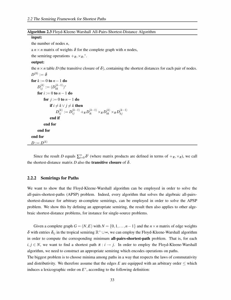
2.2 The Semiring Framework for Shortest Paths
Algorithm 2.3 Floyd-Kleene-Warshall All-Pairs-Shortest-Distance Algorithminput:the number of nodes n,
a n×n matrix of weights δ for the complete graph with n nodes,the semiring operations +R,×R,
∗.
output:the n×n table D (the transitive closure of δ ), containing the shortest distances for each pair of nodes.
D(0) := δfor k := 0 to n−1 do
D(k)i j := (D(k−1)
kk )∗
for i := 0 to n−1 dofor j := 0 to n−1 do
if i 6= k∨ j 6= k thenD(k)
i j := D(k−1)i j +R D(k−1)
ik ×R D(k)kk ×R D(k−1)
k j
end ifend for
end forend forD := D(k)
Since the result D equals ∑∞i=0 δ i (where matrix products are defined in terms of +R,×R), we call
the shortest-distance matrix D also the transitive closure of δ .
2.2.2 Semirings for Paths
We want to show that the Floyd-Kleene-Warshall algorithm can be employed in order to solve theall-pairs-shortest-paths (APSP) problem. Indeed, every algorithm that solves the algebraic all-pairs-
shortest-distance for arbitrary ω-complete semirings, can be employed in order to solve the APSP
problem. We show this by defining an appropriate semiring, the result then also applies to other alge-braic shortest-distance problems, for instance for single-source problems.
Given a complete graph G = (N,E) with N = 0,1, . . . ,n−1 and the n×n matrix of edge weightsδ with entries δi j in the tropical semiring R+∪∞, we can employ the Floyd-Kleene-Warshall algorithm
in order to compute the corresponding minimum all-pairs-shortest-path problem. That is, for eachi, j ∈ N, we want to find a shortest path π : i → j. In order to employ the Floyd-Kleene-Warshall
algorithm, we need to construct an appropriate semiring which encodes operations on paths.
The biggest problem is to choose minima among paths in a way that respects the laws of commutativityand distributivity. We therefore assume that the edges E are equipped with an arbitrary order ≤ which
induces a lexicographic order on E∗, according to the following definition:
33
Graph Algorithms and Persistent Arrays
Definition 6 Let (X ,<) be some ordered set. The lexicographic order <l on X∗ is defined by v <l w
for all v,w ∈ X ∗ with |v| < |w| and for all x,y ∈ X by x <l y if and only if x < y. For all other strings
of the form xv,yw with |v| = |w| for x,y ∈ X and v,w ∈ X ∗ we define recursively xv <l yw if and only if
either x < y or if otherwise x = y and v<l w.
For any string v = v0 · · ·vk ∈ E∗, vi ∈ E we define δ (v) := ∏ki=1 δ (vi). Note that when v happens to
be a valid path, then δ (v) is its cost. We add an absolute maximum value ∞ to the set E ∗, that is
∞ is lexicographically larger than any v ∈ E ∗ and δ (∞) := ∞. We define the binary operation min :
(E∗∪∞)× (E∗∪∞)→ E∗∪∞ as
min(v,w) :=
v, if δ (v)< δ (w)
v, if δ (v) = δ (w) and v is lexicographically strictly smaller than w
w, else
for v,w ∈ E∗. One can verify that (E∗∪∞,min,∞) forms a commutative monoid. Furthermore, (E ∗∪∞,min, ·,∞,ε) forms a ω-complete semiring, where v ·w is ∞ if ∞ ∈ v,w, and otherwise · is the usual
concatenation of strings. Indeed, · is associative with annihilator ∞ and neutral element ε , so it remainsto verify the distributive laws. Since both distributive laws can be verified in a similar way, we only
show
a ·min(b,c) = min(a ·b,a · c), for all a,b,c ∈ E ∗∪∞ .
Indeed, if a = ∞ then both sides will evaluate to ∞ and if b = ∞, then both sides evaluate to a · c, andsimilar for c = ∞. So let us assume a,b,c ∈ E ∗. If δ (b)< δ (c), then δ (a ·b)< δ (a ·c), hence both sides
evaluate to a ·b. If δ (b) = δ (c) and b is lexicographically smaller that c, then δ (a ·b) = δ (a ·c) and a ·bwill be lexicographically smaller that ac, hence both sides evaluate to a ·b. The same if we change the
roles of b and c. In the remaining case b = c, both sides will evaluate to a ·b.
Note that the semiring is ω-complete and that for v ∈ E ∗ it is v∗ = minε ,v,vv, . . . = ε . In order
to employ the Floyd-Kleene-Warshall algorithm, we start with the n× n matrix δ ′ with the entries
δ ′i j := (i, j), that is, each entry δ ′i j is the edge from i to j. Note that the semiring (E ∗∪∞,min,,∞,ε)
contains invalid paths. However, if we start the Floyd-Kleene-Warshall algorithm on δ ′, it computes for
each pair i, j ∈ N:
D(i, j) = minπ1···πk:i→ j
k
∏i=1
δi j = minπ1···πk:i→ j
k
∏i=1
πi = minπ : i→ j
According to the definition of the operation min, D(i, j) is the lexicographically first among all mini-mum paths π : i→ j.
If two paths π,π ′ have the same cost, then choosing the lexicographically first one is an expensiveoperation. In the worst case, we have to make O(m) pairwise comparisons of edges, where m is the
minimum length of π,π ′. On the other hand, in many applications it is sufficient to compute one of the
34

2.2 The Semiring Framework for Shortest Paths
shortest paths for each pair i, j ∈ N, we do not care whether it is the lexicographically first one or not.
What we actually want is to identify all paths π : i→ j with equal cost, such that the operation min canchoose in an algorithmically convenient way (even probabilistically) among paths of minimum cost.
The easiest way would be to construct a semiring that identifies all paths of equal costs, such that inan implementation, min chooses among all valid representations. The problem is that our equivalence
relation is too coarse: As an example, two paths π : i→ j and π ′ : i′ → j′ might by equivalent with
respect to their cost, but still it is i 6= i′ or j 6= j′. If the equivalence class of the shortest path from i to j
is represented by a path π ′ : i′→ j′ with i 6= i′ or j 6= j′, the result will not be of any use anymore. We can
ensure that this does not happen by inspecting the algorithm. In the case of the Floyd-Kleene-Warshallalgorithm this is not very difficult, but of course this does not take any advantage of the concept of a a
semiring as an interface for generic shortest-distance algorithms.
An alternative way is to define a semiring with built-in “type-safety", which only allows to concate-nate or to compute minima of compatible paths and otherwise yields an error-value ⊥.
For i, j ∈ N and x ∈ R∪∞ let
[i j;x] := π : i→ j : δ (π) = x
be the set of all paths π from i to j with cost x. We set
P(G) := [i j;x] : i, j ∈ N∧ x ∈ R∪∞∧ [i j;x] 6= /0
and Π(G) := P(G)∪∞,ε ,⊥. We want to define the two binary operations inf, · : Π(G)×Π(G)→Π(G) such that Π(G) = (Π(G), inf, ·,∞,ε) is a semiring.
On Π(G), we define the following partial order <: ⊥ and ∞ are absolute minimum and maximum,that is ⊥≤ a ≤ ∞ for all a ∈ Π(G). For ε , we define [ii,0] < ε for all i ∈ N. Finally, for all i, j ∈ N,
we define [i j;x]< [i j;y] if and only if x< y. All other pairs of values from Π(G) are incomparable by<.
For a,b ∈Π(G), we let inf(a,b) take the infimum of a,b with respect to the previously defined order
< on Π(G). One can show that for our specific <, such an infimum exists and that it is unique. Then
(Π(G), inf,∞) is a commutative monoid with ∞ being its neutral element.For a,b ∈ Π(G), we now define a · b: If ∞ ∈ a,b, we set a · b := ∞, hence ∞ annihilates. For all
other values, ⊥ annihilates, that is ⊥ ·a = a· ⊥=⊥ whenever a 6= ∞. Furthermore, ε acts like a neutralelement, i.e. ε · a = a · ε = a for all a ∈ Π(G). In the remaining cases assume a = [ia ja;x] ∈ P(G) and
b = [ib jb;y] ∈ P(G) for ia, ja, ib, jb ∈ N, x,y ∈ R+∪∞. Then
[ia ja;x] · [ib jb;y] :=
[ia jb;x + y], if ja = ib
⊥, else
The result of [ia ja;x] · [ib jb;y] is again in Π(G): If there exist valid paths π : ia → ja and π ′ : ib → jbwith costs x,y respectively, and if ja = ib, then π ·π ′ is a valid path with cost x + y, hence [ia jb;x + y] is
35
Graph Algorithms and Persistent Arrays
a non-empty set and therefore in P(G).
By definition, ε is a neutral element for ·. Also, · is associative, that is a · (b · c) = (a · b) · c for alla,b,c ∈ Π(G): If ∞ ∈ a,b,c it annihilates by definition and both sides evaluate to ∞. If otherwise
⊥∈ a,b,c and a,b,c 6= ∞, then ⊥ annihilates and both sides evaluate to ⊥. Associativity is easy to
verify if ε ∈ a,b,c. If now a = [ia ja;x],b = [ib jb;y],c = [ic jc;z] ∈ P(G), then both sides evaluate to[ia jc;x + y + z] if ond only if ja = ib and jb = ic, otherwise they evaluate to ⊥.
In order to show that Π(G) = (Π(G), inf, ·,∞,ε) is a semiring, it remains to show that the two laws
of distributivity hold. Since both laws can be verified in essentially the same way, we will only show
a · inf(b,c) = inf(a ·b,a · c), for all a,b,c ∈Π(G) .
First we assume ∞ ∈ a,b,c. If a = ∞, both sides evaluate to ∞. If b = ∞, then both sides evaluate toa · c because of a ·∞ = ∞. The same with c = ∞.
If a,b,c 6= ∞ but a =⊥, then both sides evaluate to ∞ if b = c = ∞, and to ⊥ otherwise. If a,b,c 6= ∞ andb =⊥ or c =⊥, both sides evaluate to ⊥. If a = ε then both sides evaluate to inf(b,c). If a = [ia ja,x] for
ia, ja ∈ N and x ∈ R+∪∞ and b = ε we distinguish the following cases: First, if c = ε then both sides
will evaluate to a. Secondly, if c = [ic jc,z] for ic, jc ∈N and z∈R+∪∞, then if ja 6= ic we get⊥ on bothsides. If on the other hand ja = ic, then we get a on both sides if and only ic = jc, otherwise we get ⊥.
It remains to show distributivity for a,b,c ∈ P(G). So assume that a = [ia ja;x],b = [ib jb;y],c = [ic jc;z] ∈P(G). Under this assumption, we observe that none of the subterms of a · inf(b,c) and inf(a ·b,a ·c) canevaluate to ∞, hence ⊥ will annihilate whenever it occurs during evaluation. Indeed, if ja = ib = ic and
jb = jc, then both sides evaluate to [ia jb,x + infy,z], otherwise they evaluate to ⊥.
Finally, one can verify that the semiring Π(G) = (Π(G), inf, ·,∞,ε) is ω-complete, and for [iaib;x] ∈P(G) it is
[iaib;x]∗ =
ε , if ia = ib⊥, else
,
and ∞∗ = ε∗ = ε and ⊥∗=⊥.
As we have seen, Π(G) = (Π(G), inf, ·,∞,ε) is a semiring. Each [i j : x] ∈ P(G) can be represented
by a path π : i→ j with cost x, in form of a persistent array plus a number x ∈ R+∪∞. This permits
efficient implementation of the operations · and inf. The Floyd-Kleene-Warshall algorithm, operatingon Π(G), will then yield a representation for one of the shortest paths for all pairs i, j ∈ N. In order
to employ the Floyd-Kleene-Warshall algorithm, we start with the n× n matrix δ ′ with the entries
36

2.3 All Pairs-Shortest-Paths and Successor Matrices
δ ′i j := [i j;δ (i, j)], where [i j;δ (i, j)] is represented by the single edge (i, j) of cost δ (i, j). If we start the
Floyd-Kleene-Warshall algorithm on δ ′, it computes for each pair i, j ∈ N:
D(i, j) = infπ1···πk :i→ j
k
∏i=1
[πi;δ (πi)]
= infπ:i→ j
[i j;δ (π)]
= [i j; infδ (π)|π : i→ j] = [i j;minδ (π)|π : i→ j]
Since in our implementation [i j;minδ (π)|π : i→ j] is represented as a valid path π : i→ j with cost
minδ (π)|π : i→ j, the matrix D gives us a solution of the APSP problem for G,δ .
2.3 All Pairs-Shortest-Paths and Successor Matrices
We have seen how persistent arrays under concatenation can be fitted into the semiring framework of
Floyd-Kleene-Warshall’s all-pairs-shortest-path (APSP) algorithm. The Floyd-Kleene-Warshall algo-
rithm will compute a matrix of shortest paths by using O(n3) array concatenations. In some cases, thereexist faster algorithms. For instance, R. Seidel’s algorithm [Sei 95], which is originated in preceed-
ing work of Alon, Galil, and Margalit, reduces the APSP problem for undirected unweighted graphsto boolean matrix multiplication. The fastest known algorithm for multiplying two n× n boolean ma-
trices is due to Coppersmith and Winograd and runs in O(n2.376) time (see [CoWi 90]) while Seidel’s
algorithm introduces an additional factor of O((logn)2). We will not discuss Seidel’s algorithm in thisthesis, a good explanation of the algorithm can be found in [MoRa 95]. The result of an APSP instance
is commonly represented as successor martix, permitting reconstruction of the shortest paths.
The purpose of this section is to show that there is no need for the effort of adapting the inner loops ofSeidel’s algorithm in order to represent the result as a matrix of persistent arrays. Instead, we will show
how any n×n successor matrix can be transformed into a matrix of persistent arrays in O(n2 logn) time.
Definition 7 Let G = (N,E) be a graph. Assume the set of nodes is numbered, i.e. N = 0,1, . . . ,n−1.A successor matrix for G is a n× n matrix R with entries in ∞,0,1..n− 1 such that for 0 ≤ i, j < n, if
i = j then Si j = j. For i 6= j it is Si j = ∞ if and only if i, j ∈ N are disconnected and Si j ∈ N if and only
if there exists a simple path π : i→ j such that π traverses the node Si j directly after i.
In this section, paths are again represented as sequences of edges. In order to obtain a path from i to j,
and assuming that i, j are connected, we only need to go from i to Si j and then continue successivelyuntil we reach j. Indeed, for any instance of the APSP problem there exists a solution which can be
represented as a successor matrix (but not every solution).
The task is to transform a given n× n successor matrix R in such a way that we get a n× n matrix
P with entries in N∗∪∞ such that for i, j ∈ N, Pi j = ∞ if and only if i, j are disconnected, else Pi j is ashortest path π : i→ j.
The idea is to compute matrices S(k), k = 0..dlog ne, starting with S(0) = S. For disconnected i, j ∈N, all
37

Graph Algorithms and Persistent Arrays
S(k)i j , k = 0..dlog ne, are ∞. Now assume that i, j ∈ N are connected and let π = π0 . . .πm : i→ j be the
path from i to j which is described by the successor matrix R. Then the entry S(k)i j of matrix k is defined
to be the 2kth node π2k of the path π if 2k ≤m, and otherwise S(k)i j = j. At the same time, we maintain a
n×n matrix P(k), such that if i, j are connected, then P(k)i j ∈N∗ is a shortest path from i to S(k)
i j . Note that
a shortest path which is described by a successor matrix can never traverse more than n edges, henceafter k ≤ logn iterations we have that P(k)
i j is a shortest path from i to S(k)i j = j.
Algorithm 2.4 Transforming a successor matrix R into a matrix P of paths
S(0) := R
for i := 0 to n−1 dofor j := 0 to n−1 do
if i = j thenP(0)
ii := εelse if Si j = ∞ then
P(0)i j := ∞
elseP(0)
i j := [i,Si j ]
end ifend for
end forfor k := 1 to dlog ne do
P(k) := P(k−1)
S(k) := S(k−1)
for i := 0 to n−1 dofor j := 0 to n−1 do
if i 6= j∧S(k−1)i j 6= ∞∧S(k−1)
i j 6= j thenR := S(k−1)
i j
P(k)i j := P(k−1)
i j ·P(k−1)s j
S(k)i j := S(k−1)
s j
end ifend for
end forend forP := P(dlogne)
P(0) can be computed in O(n2) time, and since each iteration needs n2 many concatenations of
persistent arrays, the total running time is O(n2(log n)2). A more detailed analysis reveals that for eachpair i, j, all except one of the dlog ne many concatenations either involve an empty array or two arrays
represented by trees of equal height (if we use our implementation of persistent arrays as AVL trees).
38

2.4 Related Work
Those are special cases of concatenation which can be handled in O(1) time. So finally, the time bound
for our algorithm is actually O(n2 logn).The space requirements are bounded by the execution time of the algorithm, hence the resulting matrix
P requires O(n2 logn) space.
Corollary 16 Given a n× n successor matrix S for a graph G = (N,E) and a monoid homomorphism
h : E∗→M, it is possible to compute h(π) simultaneously for all shortest paths π which are represented
by S. The computation requires O(n2 logn) time plus the time needed for O(n2 logn) multiplications in
M and for computing O(|E|) images h(x), x ∈ E.
PROOF: In algorithm 2.4, we can maintain the images h(π) of paths. The additional costs involved are
exactly those stated in the theorem. Another approach would be to modify algorithm 2.4 in such way
that it computes the images h(π) directly. 2
2.4 Related Work
The main contribution of the first section of this chapter is a method for maintaining path information
within ET trees. ET-trees have been introduced by Henzinger and King, see [HeKi 99]. Another datastructure for dynamic trees are topology trees, which have been proposed by Fredrickson, see [Fre 85].
The article [AHLT 03] by Alstrup, Holm, de Lichtenberg, and Thorup gives an alternative description
called top trees. There the authors show how to maintain diameter, center and several other tree parame-ters. The article [EGI 99] by Eppstein, Galil, and Italiano gives a extensive overview on dynamic graph
algorithms. It should be noted that our implementation of dynamic trees, which uses ET trees, does
not fully implement Sleator and Tarjan’s axiomatic interface for dynamic trees, since it does not allowefficient updates of edge-weights along a path. On the other hand, ET trees have been used by Holm, de
Lichtenberg, and Thorup ([HLT 01]) for dynamic connectivity problems on general undirected graphs,where the total costs per update are O((logn)2). It is reasonable to assume that the additional overhead
for maintaining path information by persistent arrays does not harm much in those cases.
The observation 14 is a generalization of equivalent results for disjoint trees.The semiring framework for Floyd-Kleene-Warshall’s algorithm can be found in many textbooks, see
for instance [AHU 74] and the first edition of [CLRS 01]. The article by M. Mohri [Moh 02] shows sev-
eral semirings in context of shortest-path and shortest-distance problems. The construction of a semiringfor paths represented as persistent arrays is by the author of this thesis.
Many APSP problems represent their solutions as successor — or alternatively predecessor — matrices.The algorithm 2.4 for transforming a successor matrix to a matrix that represents paths as persistent
arrays is new in this thesis. Remarkable is the small additional space overhead, since persistent arrays
are much more versatile for subsequent processing of the result.
39


Chapter 3
Homomorphisms on Arrays
A compact representation of large arrays in memory is not very useful if we cannot efficiently extract
some information from it. The homomorphism technique provides means for computing with exponen-
tially large, persistent, arrays. There are many functions on arrays which can be considered as homo-morphic images, or where homomorphic images help during the course of computation. In particular
we provide probabilistic polynomial-time algorithms for equality test and lexicographic comparision.We also provide deterministic polynomial-time algorithms for sorting elements and for the generalitzed
state machine.
The homomorphism technique for arrays is also useful for algorithm design. This has already beenemployed in the field of parallel algorithms, in computer algebra, and many other fields of algorithm
design. We give some further examples in this chapter, in particular interactive line breaking.
3.1 Algorithms on Large Arrays
3.1.1 Polynomial Evaluation and Inequality Tests
Let R = (R,+, ·,0,1) be a commutative semiring. By R[z] we denote the semiring of single-variabled
polynomials over R. We wish to evaluate a given polynomial f (z) = anzn + an−1zn−1 + . . .+ a0 ∈ R[z]
of degree n for some fixed value x of the variable z, adaptively to changing coefficients a0, . . . ,an:
Let A ∈ R∗ be some array of length |A| = n + 1 with elements A[i] = ai, i = 0..n, from R. The corre-
sponding polynomial of degree dA = n is the polynomial fA with ai as the coefficient for the ith powerof its argument. For some fixed x ∈ R, we want to evaluate
fA(x) := anxn + an−1xn−1 + . . .+ a0 .
On A we allow update operations such as changing one of the coefficients a i, i = 0..n. During updates,
we wish to maintain the polynomial’s value at x: If A′ is the array that results from A by changing ai toa′i, we want to get immediatly the new value for fA′(x). If R is a ring, the new value can be computed by
fA′(x) = fA(x) + (a′i−ai)xi .
41
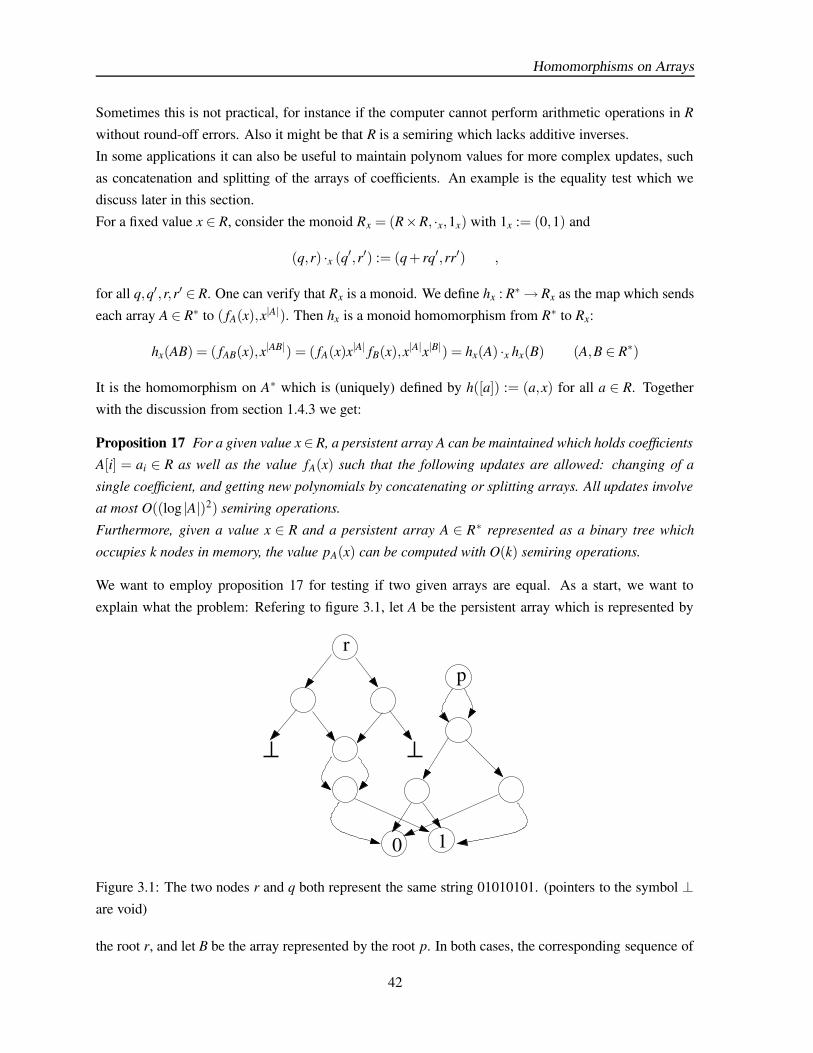
Homomorphisms on Arrays
Sometimes this is not practical, for instance if the computer cannot perform arithmetic operations in R
without round-off errors. Also it might be that R is a semiring which lacks additive inverses.In some applications it can also be useful to maintain polynom values for more complex updates, such
as concatenation and splitting of the arrays of coefficients. An example is the equality test which wediscuss later in this section.
For a fixed value x ∈ R, consider the monoid Rx = (R×R, ·x,1x) with 1x := (0,1) and
(q,r) ·x (q′,r′) := (q + rq′,rr′) ,
for all q,q′,r,r′ ∈ R. One can verify that Rx is a monoid. We define hx : R∗→ Rx as the map which sends
each array A ∈ R∗ to ( fA(x),x|A|). Then hx is a monoid homomorphism from R∗ to Rx:
hx(AB) = ( fAB(x),x|AB|) = ( fA(x)x|A| fB(x),x|A|x|B|) = hx(A) ·x hx(B) (A,B ∈ R∗)
It is the homomorphism on A∗ which is (uniquely) defined by h([a]) := (a,x) for all a ∈ R. Together
with the discussion from section 1.4.3 we get:
Proposition 17 For a given value x∈R, a persistent array A can be maintained which holds coefficients
A[i] = ai ∈ R as well as the value fA(x) such that the following updates are allowed: changing of a
single coefficient, and getting new polynomials by concatenating or splitting arrays. All updates involve
at most O((log |A|)2) semiring operations.
Furthermore, given a value x ∈ R and a persistent array A ∈ R∗ represented as a binary tree which
occupies k nodes in memory, the value pA(x) can be computed with O(k) semiring operations.
We want to employ proposition 17 for testing if two given arrays are equal. As a start, we want to
explain what the problem: Refering to figure 3.1, let A be the persistent array which is represented by
0 1
p
r
Figure 3.1: The two nodes r and q both represent the same string 01010101. (pointers to the symbol ⊥are void)
the root r, and let B be the array represented by the root p. In both cases, the corresponding sequence of
42

3.1 Algorithms on Large Arrays
elements is seq(A) = seq(B) = 01010101, hence we would consider A and B being equal. When using
persistent arrays, we do almost never care about their actual representation in memory. Generally wesay that two persistent arrays are equal, whenever the corresponding sequence of elements are equal.
The problem of deciding equality arises with very large arrays, in particular those which’s length growsexponentially in the number of nodes. In this case, iterating through the sequence of elements and
making a one-by-one comparision is unfeasible.
There exists a common technique which helps us to provide a probabilistic (in)equality test: Given
two arrays A = [a0, . . .an−1], B = [b0, . . .bn−1] of equal length n and an errorbound ε > 0, we choose arandom number p. Then we compute fingerprints of both arrays modulo p in such a way that if A and B
are equal, the fingerprints always coincide. If A and B are unequal, the probability that the fingerprints
are different is at least 1− ε .The resulting algorithm is of onesided-error Monte-Carlo type, i.e. it always terminates and for equal
A,B, it always yields the correct answer by comparing both fingerprints. Termination is guaranteed in
time polynomial in the size of the represantation of A,B as binary trees and the number of leading zerosin the binary (fixed-point) representation of ε .
When dealing with probabilistic algorithms, the underlying machine model is a RAM with a sequence
of uniformly distributed independent random bits X0X1X2 . . .. This allows us (in many practical cases)
to consider all results during the computation as random variables over the discrete probability spacewhich corresponds to the atomic events X0,X1, . . . ,Xk, where k is the maximum number of used random
bits on the given input. Note that for Las-Vegas type algorithms, the model is slightly more involved
since the number of random bits can be unbounded. For more details about discrete probability andprobabilistic algorithms, see the [MoRa 95].
Assume that the number of distinct elements of A and B is at most m, i.e.
m := |ai,bi : i = 0..n−1| .
It is easy to deduce m from the binary tree representation of A,B by traversing its leave nodes. We canthen replace each element from A,B by a unique identifier from the set of numbers 0..m− 1. Without
loss of generality, from now on we assume that all elements are numbers between 0 and m−1. Now A
and B are equal if and only if the corresponding polynomials fA, fB are equal at point m:
A = B ⇔ fA(m) = fB(m)
The reason is that the value fA(m) = ∑n−1i=0 aimi is the number which A = [a0, . . . ,an−1] represents in
m-adic representation, which is — for fixed length n — unique. The same for B and fB(m). Proposition
17 ensures that the values fA(m), fB(m) can be computed with a number of operations which growspolynomially in n. The only problem is that the number of bits needed can be as much as O(n), which
can be exponential in the size of A and B’s representation. Instead of computing fA(m), fB(m) over the
43

Homomorphisms on Arrays
integers, we perform all computations modulo a random number p. When the number of bits for p is
polynomially bounded, we can compute the fingerprints fA,p := fA(m) mod p and fB,p := fB(m) mod p
polynomial time. We then have
A = B ⇒ fA,p = fB,p .
The other direction is, of course, not true in general. However, if fA(m) = fB(m) modulo p, then p
divides | fA(m)− fB(m)|, which has at most
log2 | fA(m)− fB(m)| ≤ log2(mn+1)≤ n′
prime devisors for n′ := (n + 1) log2 m. Hence if p happens to be a prime number, then the fingerprints
fA,p, fB,p can only coincide if p is among the prime devisors of | fA(m)− fB(m)|, from which there are
at most n′ many. The trick is to choose p as a prime number uniformly from an intervall 0..τ whereτ is large enough such that the probability that p is among the prime devisors of | fA(m)− fB(m)| is
negligible.
The prime number theorem ensures that there exist enough primes already for small k: For an integerx, denote the number of primes smaller or equal to x by π(x). W will discuss its application in such a
way that an implementation with guaranteed errorbounds is possible. We use Rosser and Schoenfeld’sinequality
lnx− 32<
xπ(x)
< lnx− 12,
from whichx
2lnx≤ π(x)
follows. We then choose τ ≥ 5n′ε−1 ln(n′ε−1). The number of bits for the binary representation of τdepends only polynomially on n (since n′ = (n + 1) log2 m and m≤ n) and the number of leading zeros
in ε’s fixed-point representation. If n′ ≤ 10 we can decide equality by comparing the array elementsone-by-one. If ε > 0.1 it does not do any harm to test equality for a better errorbound. Hence without
loss of generality, we can assume n′ ≥ 10 and ε ≤ 0.1 and obtain
Prob( fA = fB | A 6= B∧ p is prime) =n′
π(τ)
≤ 2n′ lnττ
≤ 2n′ ln(5n′ε−1 ln(n′ε−1))
5n′ε−1 ln(n′ε−1)
≤ 2n′ ln(6n′ε−1)
5n′ε−1 ln(n′ε−1)
=2n′(ln6 + ln(n′ε−1))
5n′ε−1 ln(n′ε−1)
≤ 2n′(2ln(n′ε−1))
5n′ε−1 ln(n′ε−1)
=45
ε ≤ ε
44

3.1 Algorithms on Large Arrays
when fA, fB are interpreted as random variables1 . There exist polynomial-time probabilistic algorithms
which generate, on input k ∈ N, and errorbound ε > 0 a prime number candidate p with k bits, inthe following sense: For the returned candidate p (a random variable which depends on the machine’s
random bits)
Prob(p is not prime)≤ ε ,
and Prob(p = p1) = Prob(p = p2) for all prime numbers p1, p2 ≤ 2k . See for instance [MoRa 95].Combining such an algorithm with the computation of the fingerprints fA, fB yields an errorbound
Prob( fA = fB | A 6= B) ≤ Prob( fA = fB | A 6= B∧ p is prime) + Prob(p is not prime) ≤ 2ε .
In practice, software libraries often provide a candidate-tester pair of Monte-Carlo type functions for
prime number generation for with a built-in errorbound α > 0. That is, the probabilistic functionCANDIDATEPRIME(k) yields a number with k bits which is prime with probability at least 1−α . The
probabilistic function TESTPRIMALITY(p) decides wether p ∈ N is a prime. The primality test mayyield the wrong answer with probability ≤α but is always “yes" if p is prime. In order to obtain a smaller
errorbound ε ≤ α , one can still use such a candidate-tester pair: We generate up to r≥ logα(ε/2) prime
candidates, each one with errorbound α , from which we choose the first one which passes r primalitytests (with errorbound α). If no candidate passes its r primality tests, we return any number we like.
The probabilty that the chosen candidate is a prime number is then at least 1− ε .
3.1.2 Lexicographic Comparison
The probabilistic equality test can be adapted to a probabilistic lexicographic comparison. The mainproblem is, for two unequal arrays A = [a0, . . . ,an−1], B = [b0, . . . ,bn−1] to find the first index i such that
ai 6= bi. This is the same as finding the longest equal prefixes [a0, . . . ,ai−1] = [b0, . . . ,bi−1]. We can findi by recursively splitting the search interval 0..n−1 into two parts 0..i−1 and i..n−1 of approximately
the same length and continue our search in the first of the two intervals for which the values of A and B
differ. This binary search will take time which is polynomial in the size of the array’s binary searchtreerepresentation. By calling each equality test with errorbound ε/k, where k = dlog ne is the maximum
number of comparisons, the resulting errorbound will be less than the probability of error for at least
one of the k tests, which then is ≤ ε .
3.1.3 Equality Tests for Arrays which May Contain Arrays
The probabilistic equality test can be generalized to an equality test for composite structures based on
persistent arrays. Until now we usually considered sequences over some ground set X . However, whenwe use persistent arrays as a basic type of a programming language, there is little reason not to allow
arrays themselves to be elements of other arrays.
1In the literature it is common to avoid the formal details when switching from some object to its interpretation as a randomvariable.
45

Homomorphisms on Arrays
Let X be a finite set of atoms. (For instance the set of all instances of primitive types which fit into
a register). The universe over X is the set U (X) which is recursively defined as:
U0(X) := X
Ui+1(X) := (⋃
j=0..i Ui(X))∗
U (X) :=⋃
i=0,1,2,...Ui(X)
If A,B ∈U (X) they can be transformed into arrays A′,B′ ∈ X ∪(,)∗ in polynomial time such that A
equals B if and only if A′ equals B′: We assume (,) 6∈ X ∗ and flatten an array A ∈ U (X) to an array
A′ ∈ X∗ by recursively replacing each non-atom [x1,x2, . . . ,xn] by the sequence (x1x2 · · ·xn). For anbinary tree representation, this can be achieved in polynomial time by traversing the tree.
3.1.4 Sorting of Elements
Let A = [a0, . . . ,an−1] be an array of elements ai ∈ X , where X is linearly ordered by the relation ≤. Our
goal is to sort A, i.e. to create an array A′ = [a′0, . . . ,a′n−1] with
a′0 ≤ a′1 ≤ . . .≤ a′n−1
such that for each x ∈ X , its number of occurences in A equals its number of occurences in A ′. This can
be achieved by the following algorithm: First, we compute the set
XA := ai : i = 0..n−1
of all elements of A. This can be done by traversing the tree which represents A or, alternatively, by the
applying the homorphism which maps an array to the set of its elements. In the next step, we computefor each x ∈ XA its number of occurences in A by computing the image hx(A) for the homomorphism
hx : X∗→ (N,+,0) defined by
hx(y)
1, if x = y
0, else(y ∈ X).
Now, for each element x∈ XA, we create an array representing the sequence xhx(A) by fast exponentation,
and then we concatenate these arrays in the right order. Note that actually we only need to sort the setXA of all elements of A, which has at most the size of the binary tree which represents A.
3.1.5 Generalized State Machine and Acceptor
Let X be some finite alphabet. A generalized state machine M which transforms strings from X + tostrings from X ∗ is a tuple M = (X ,S,s0,δ1,δ2). Here, S is a finite set of states, s0 is the initial state,
and δ1 : S×X→ S,δ2 : S×X→ X∗ constitute M’s program and describe the tranducer’s behavior on aninput string u ∈ X+: We can extend δ1,2 on S×X+ by recursively defining
δ1(s,ux) := δ1(δ1(s,u),x)
46
3.2 Algorithm Design
and
δ2(s,ux) := δ2(s,u)δ2(δ1(s,u),x)
for u ∈ X+, x ∈ X and s ∈ S. For an input u ∈ X +, we set M(u) := δ2(s0,u).
A generalized state machine M = (X ,S,s0,δ ) can also be defined in terms of a homomorhismhM : X∗→ SS× (X∗)S. Multiplication in SS× (X∗)S is defined by
(( f1, f2) · (g1,g2))(s) := (g1( f1(s)), f2(s)g2( f1(s))) (s ∈ S)
for f1,g1 ∈ SS and f2,g2 ∈ (X∗)S. The neutral element is (s 7→ s,s 7→ ε). The homomorphism hM is
defined by
hM(x) := (s 7→ δ1(s,x),(s 7→ δ2(s,x)) (x ∈ X) .
Now, for a string u ∈ X +, we get
hM(u) = (s 7→ δ1(s,u),s 7→ δ2(s,u)) ,
hence (hM(u))(s0) = (δ1(s0,u),M(u)). The elements from the monoid SS× (X∗)S can be represented
in size polynomial in |S| ·maxs∈S,x∈X δ2(s,x), which is a natural measure for the size of M. Hence themultiplication as defined above can be performed in polynomial time. Together with the results from
section 1.4.3, we get a polynomial time algorithm for computing M(u) when u is the sequence of ele-
ments of a persistent array represented by a binary tree. Note that in an implementation, it will be wisenot to follow the homomorphism technique too doggedly. It is generally better to traverse left subtrees
first in the representation of the array and only compute transitions which really occur when processing
the input string.
A deterministic finite acceptor M can be considered as a special generalized state machine, whichaccepts an input string u ∈ X + if and only if M(u) ends with “yes" (symbolizing and accepting state).
Only slight modifications will allow us to search for patterns described by a deterministic finite automa-
ton in polynomial time.
3.2 Algorithm Design
In this section we want to give two further examples for the use of homomorphisms or binary trees for
on arrays as a tool in algorithm design. Since the idea has been employed in many areas of algorithmdesign since long, we only introduce two applications which evolved during our own research.
3.2.1 Poisson Trials
A Poisson trial with success probabilty p is a random experiment with only two possible outcomes:
0 with probability 1− p and 1 with probability p. If a Poisson trial with fixed success probability is
47
Homomorphisms on Arrays
repeated independently, it is called a Bernoulli trial. An application of a Bernoulli trial is for instance
the simulation of a system where different events might occur any time with constant probability. Moreformally, let the random variables Xi, 0 ≤ i < n describe n independent Poisson trials, each one with
success probability pi. We want to generate a random sample and collect those trials with positive out-come. In other words, the task is to pick each item i ∈ 0,1, . . .n−1 with probabilty p i independently
and then put the chosen items into a set L. The generic algorithm is algorithm 3.2.1.
Algorithm 3.2.1 The generic algorithm for drawing a sample of n independent trials:
L := /0
for i:=0 to n−1r := RANDOM[0,1]
if r ≤ pi then L := L∪iendfor
We assume that RANDOM[0,1] generates uniformly and with high enough precision a random float-
ing point number in the intervall [0..1].
Algorithm 3.2.1 typically occurs implicitly in simulations of stochastic processes and also in some
randomized algorithms. Often the algorithm needs to be repeated many times, so each Poisson trial X i
becomes a Bernoulli trial. If the pi are much smaller than 1/2, iterating through all pi for only a small
amount of items that are actually choosen becomes inefficient — we generate a low-entropy sample
with a large number of random bits.For example, when simulating system in a critical environment, such as computers with faulty mem-
ory cells, algorithm 3.2.1 becomes very time-consuming if the pi are small: it generates O(n) random
numbers for only a small amount of positive outcomes. If the drawing of the samples is repeated manytimes, it might be better to use analytic techniques in order to generate samples with positive outcome
for each Xi ahead of time and to queue them up until needed.2 This might be the fastest way if we drawsamples unconditionally, but it does not allow to draw samples with a fixed number of positive outcomes
in order to study the system under extremal conditions. We could go back to algorithm 3.2.1 and repeat
it until the drawn sample has the required number of positive outcomes, however this turns out to beunfeasible if the pi are small.
The algorithm that we describe here makes better use of the random bits than algorithm 3.2.1 does
and allows to draw samples according to a required number of positive outcomes: Let the Xi, 0≤ i < n,be our n Poisson trials, i.e. independent random variables where Xi = 0 with probability 1− pi and
Xi = 1 with probability pi. Our algorithm first generates a random number e with the distribution of Y =
2For the analytic properties of Bernoulli trials see [Knu 98]
48

3.2 Algorithm Design
X0 + . . .+ Xn−1. Then it picks exactly e items from the set 0..n−1 according to their probabilities. In
order to fasciliate this, the algorithm makes use of a recursive splitting of Y which has to be computed ina preprocessing stage. We describe both, the preprocessing and the algorithm for choosing the numbers,
in the next section.It is well-known that the distribution of Y = X0 + . . .+ Xn−1 is the n-fold convolution of the prob-
abilities pi and therefore can be computed with O(n(log n)2) floating point operations by using fast
Fourier tranformation (FFT) for the convolution products. The consideration of floating point preci-sion and roundoff errors is application-specific. However, depending on the randomized algorithm, we
might want to bound the required floating point precision as well as the number of random bits that areneeded. In stochastic simulations, as long as we do not force extremely rare events to occur (in this case
an outcome for Y very far from the expectation E[Y ]), we can virtually ignore the effect of floating point
precision and use the built-in machine floating point arithmetic. As a remark, results from simulationsmust be regarded with high scepticism anyway. Both, this algorithm and the generic algorithm 3.2.1
depend on the quality of the random number generator.
Preprocessing
We recursively split the sequence of random variables Xi in such a way that its partitions form a balanced
binary tree: For 0≤ i≤ j< n we define Yi j := Xi +Xi+1 + . . .+X j. Thus we have Y = Y0,n−1 and Xi = Yii
for 0≤ i < n. Also, for 0≤ i≤ k ≤ j < n we have
Prob(Yi j = c) = ∑a+b=c
Prob(Yik = a)Prob(Yk j = b) . (3.1)
Now let T be the smallest set with the following properties: Y = Y0,n−1 ∈ T and for each Yi j ∈ T with
i 6= j there are Yi,b(i+ j)/2c ∈ T and Yb(i+ j)/2c+1, j ∈ T . As a consequence, all the Xi = Yii are elements ofT . Next, for all Yi j ∈ T we compute their distribution
D(Yi j) := (Prob(Yi j = 0),Prob(Yi j = 1), . . . ,Prob(Yi j = j− i + 1)) .
Since 3.1 shows that D(Yi j) is the convolution of D(Yi,b(i+ j)/2c) and D(Yb(i+ j)/2c+1, j), we can computeall the distributions in O(n(log n)2) time by using FFT for the convolution products. We store the
distributions in a binary tree such that each D(Yi j) is in the parent node of the nodes for D(Yi,b(i+ j)/2c)
and D(Yb(i+ j)/2c+1, j). This binary tree needs O(n log n) space. Finally, we integrate the distribution ofD(Y ) = D(Y0,n−1), that is, instead of D(Y ) we store the sums
i
∑k=0
(D(Y ))k =i
∑k=0
Prob(Y = k)
for all 0 ≤ i ≤ n. Note that the sum above is very sensitive to roundoff errors because some values are
extremely small compared to others. The reason why we only integrate D(Y ) is that later we want togenerate random numbers e with the distribution of Y . Other datastructures might serve the purpose bet-
ter, especially if we can not ignore rare outcomes for Y . One solution would be to split D(Y ) recursively
49
Homomorphisms on Arrays
and to store the partial sums in a binary tree. The sums are then stored relative to each other in such a
way that each one can be computed by sumation along the path from the root to its node. This allowsthat the precision — as much as the convolution procedure has left to us — at the tails of D(Y ) will not
be lost and can be used for a refined generation of e.
Choosing the Items
As already described, at first our algorithm decides how many items it will choose, i.e. is it generates a
random number e with the distribution of Y . This can be achieved by generating a random number in theintervall [0,1] with uniform distribution and then performing a binary search in the array that stores the
sums ∑ik=0(D(Y ))k (because this is only a small part of the algorithm, there is little point in replacing the
binary search by a Newton iteration). Next we call the procedure CHOOSE(i, j,e) for i = 0 and j = n−1.The procedure CHOOSE(i, j,e) picks exactly e items from the set i, i + 1, i + 2, . . . , j according to the
probabilities for Xk = 1 under the condition that Xi + . . .+ X j = e. CHOOSE(i, j,e) works as follows: Ife = 0 we pick no item at all. Otherwise we check if i = j and if yes, we have no other choice but to pick
the only possible item i (in this case e must be 1, if not something went wrong with the implementation
of the algorithm). In all other cases, we set m = b(i + j)/2c and compute the conditioned probabilitiesProb(Yim = k|Yi j = e) for k = 0,1, . . . ,e. We use Bayes’ rule:
Prob(Yim = k|Yi j = e) =Prob(Yim = k∧Yi j = e)
Prob(Yi j = e)=
Prob(Yim = k) ·Prob(Ym+1, j = e− k)
Prob(Yi j = e).
The right part of the equation follows from the independence of our Poisson trials and the fact that
Yi j = Yim +Ym+1, j. Then we generate a random number f with the distribution of Yim|Yi j = e: We in-tegrate the distribution (ie the the probabilities Prob(Yim = k|Yi j = e)), generate a random number in
[0,1] uniformly, and locate it in the integral of the distribution. The values we finally pick are the values
picked by the two subsequent calls CHOOSE(i,m, f ) and CHOOSE(m + 1, j,e− f ).
Sometimes we might wish to replace RANDOM[0,1] by a random number generator that generates(more or less perfect) random bits. In this case, we start with the interval [0,1] and choose (depending
on the outcome of the first random bit) its lower or upper half. We repeat this procedure recursively until
our interval is completely covered by two successive values of the integral of the distribution we want tosample from. Most of the time, this procedure terminates quickly. In some very rare cases (with nearly
zero probability), it can run forever but we can break up if the error is low enough.
Performance
We assume constant time for all arithmetic operations and negligible time for RANDOM[0,1]. For
N > 1 and arbitrary i, the procedure CHOOSE(i, i+N,e) takes time T (N,e)≤ ce+T(bN/2c, f )+T (N−bN/2c,e− f ), depending on the outcome of the randomly generated f . The constant c must be large
enough so that it bounds T (0,e) while at the same time ce bounds the time needed for computing the con-
50
3.2 Algorithm Design
ditioned probabilities and for generating f . Substituting the times T (bN/2c, f ) and T (N−bN/2c,e− f )
and also the times for all the other recursive calls of CHOOSE(. . .) yields
T (N,e) ≤ ce + c f + c(e− f ) + c f1 + c( f − f1) + c f2 + c(e− f − f2) + . . .
+ ce
= ce + ce + ce + . . . + ce .
Here, f1 and f2 are the outcomes for f in the first two subsequent calls. However, the maximum time
spent at the level of the first two subsequent calls sums up to c f + c(e− f ) = ce as it also happens at
each other level of our recursion, no matter what the respective outcomes for f are. Altogether we haveO(logN) times the term ce, hence T (N,e) = O(e logN). We conclude that the expected time for our
algorithm is O(E[Y ] logn). Also, we need no more than edlog ne+1 calls of RANDOM[0,1]: There are e
items to pick, which in the worst case have to be located separately by using dlog ne random numbers for
each. Hence the expected number of calls of RANDOM[0,1] is E[Y ]dlog ne+1. As previously mentioned,
the algorithm makes use of a precomputed datastructure which takes O(n log n) space and O(n(log n)2)
time for construction.
However, great savings in space and particularly in time needed for the preprocessing can be made by
observing that many entries in the joint distributions are practically zero. The maximum number ofinterest for the positive outcomes is typically much smaller than n.
Results and Suggestions
We implemented both, the generic algorithm 3.2.1 and the algorithm described here in the JAVA pro-
gramming language. We used the built-in pseudorandom number generator which generates a floating
point number in the intervall [0,1] with uniform distribution. All arithmetic was done by the machine’sfloating point unit (DOUBLEs) with no special regard to roundoff errors. Then we run both algorithms
for n = 10000 on a 800 MHz pentium processor: The generic algorithm 3.2.1 used 3.6 ms indepen-
dently of E[Y ] while the preprocessing for our algorithm used 215 ms (using a simple radix-2 FFT forthe convolution products). For E[Y ]/n = 0.0002/0.002/0.02/0.2/0.5, time consumption of our algorithm
averaged 0.033/0.18/1.07/5.59/7.31 ms respectively. This confirms our expectation that our algorithmoutperforms the generic algorithm 3.2.1 if E[Y ] is small compared to n and the number of repetitions is
large. But even for E[Y ]/n = 0.5, choosing from n = 10000 items only takes twice as much time as with
the generic algorithm. Since we can always choose all pi ≤ 0.5 and since the logarithmic factor for otherpractical values for n > 10000 will not make much difference, our algorithm appears to be comparable
to the generic algorithm in all cases with high speedup for small E[Y ]. Plus, it has the advantage that itis possible to fix the number of positive outcomes in each sample in advance.
There are, of course, other algorithms for simulating many parallel Bernoulli trials. For instance, we
could for each Xi precompute a list of future outcomes and put them into a queue. This algorithm wouldhave the advantage that it adapts naturally to updates on the set of all trials without the time-consuming
FFT. So this algorithm algorithm will be asymptotically much faster than ours. For interactive simu-
51
Homomorphisms on Arrays
lations, for instance in computer games, preparing the queue for future outcomes for each trial X i can
result in a constant-factor overhead which leads to unpleasant delays when all Xi are initialized. In thiscase we suggest to use the alg+orithm from this subsection in order to get a quick start for the initial
simulation and then preparing the queues for the adaptive algorithm in the background.
3.2.2 Interactive Line Breaking
Our next application is interactive line breaking in text processors. One way to break paragraphs into
lines is to scan the text (or part of it) from left to right and add a line break at a position with the best
penalty for the current line. This does not take into account that a good choice for the current linemight lead to a bad overall line breaking for subsequent lines, thus even leading to a suboptimal overall
solution for the whole paragraph. A very good line breaking algorithm is Knuth’s best total-fit linebreaking which works offline by constructing the best total-fit while scanning the paragraph from its
start. However, for long paragraphs this might not always be feasible for interactive text processors,
which is especially true if more complicated tasks such as score breaking, page breaking, or imagelayout have to be included.
We give here a simple version of an interactive line breaking algorithm for best total-fit solutions in the
very basic setting of inserting line breaks into paragraphs.Let X be a finite alphabet in which the (unbroken) paragraph has been written. An additional symbol
$ 6∈ X shall be understood as a line break. Given a paragraph w ∈ X ∗ the task is to find a string w′ =
w0$w1$ . . .$wn−1$wn ∈ (X ∪ $)∗, wi ∈ X∗, which breaks w = w0 . . .wn into lines such that w′ has a
minimum value for its line breaking penalty σ(w′) ≥ 0. This minimum penalty of w is denoted by
σmin(w). We have to make a few assumptions about the penalty function σ : First we asume that foran unbroken line u ∈ X ∗ we get a penalty σ(u) ≥ 0. In this case, σ(u) evaluates the appearance of the
string u layouted on a single line. Secondly, if x is of the form x = u$v for u,v ∈ (X ∪ $)∗, we assume
that the penalty function is monotone:
σ(v′)≥ σ(v)∧σ(u′)≥ σ(u) ⇒ σ(v′$u′)≥ σ(v$u)
The assumption is reasonable since it means that a line breaking cannot be made better by replacing oneof its parts by a worse broken part while leaving all other line breaks as they are.
In most texts, the maximum length of a single line is bounded by some number k. This means thatfor any given w = w1 · · ·wn, wi ∈ X with n > 2k, there must be a line break within the first k and within
the last k symbols of each feasible line breaking of w. For 1≤ i, j ≤ k, we set
δ (w, i, j) := σmin(wi+1 · · ·wn− j) .
Let u = u1 · · ·um,v = v1 · · ·vn, ui,vi ∈X be two unbroken paragraphs of length> 2k. Let ci j be some k×k
matrix over (X ∪$)∗ with σ(ci j) = δ (u, i, j) and such that ci j is a line breaking of the infix ui · · ·um− j of
u. Let di j be a similar matrix for v. Then we have
δ (uv, i, j) = minr,s∈1..k
σ(cir$um−r+1 · · ·umv1 · · ·vs−1$ds j) . (3.2)
52

3.2 Algorithm Design
Usually, when σ(cir) and σ(ds j) is known, computing σ(cir$um−r+1 · · ·umv1 · · ·vs−1$ds j) needs only to
take the line umv1 · · ·vs−1 into account. We assume O(k) time for that, but sometimes costs can be higher.
Let w be an unbroken paragraph of length n which is given as a sequence of a persistent array’s A
elements. As usual, A is represented as a binary tree and thus permits edit operations such as inser-
tion, deletion, and concatenation of paragraphs. In order to maintain a line breaking with minimum
penalty, we memorize for each inner node p of the tree representation the following information: Letu = u1 · · ·um, ui ∈ X be the infix of w which corresponds to the subtree at node p. At p, we store all val-
ues δ (u, i, j), i, j = 1..k and corresponding optimal line breakings ci j of the infix ui · · ·um− j . Accordingto equation 3.2, all those values for p depend solely on the values for its children. The computation of
each of its k2 entries needs to test k2 line breaks. Each such test involves the time O(k) for the evaluation
of the line breaking, and O(logn) time for concatenating the newly broken paragraphs. Alltogether, eachupdate on w needs O(k4(k + logn)) time for updating to a new optimal line breaking.
The whole procedure can be cast into the homomorphism-framework by identifying line breakings of
the same original paragraph which have in the same penalty. The factor k5 might appear prohibitive. Butfirst note that not all positions in a line are candidates for a line break, so k is often very small. Secondly,
by making the boundaries overlap, we can get rid of one of the two middle line breaks in equation 3.2,which saves a factor k.
3.2.3 Related Work
Decomposing arrays into trees and using monoid homomorphisms is an old but very versatile technique.
The same goes for the fingerprint technique modulo random primes. Historical notes for the latter canbe found in [MoRa 95], but we want to add that the fingerprint technique has also been adapted for
testing equality of certain binary decision diagrams. The use for persistent arrays, however, is new and
has been first described in [Bar 04].A best-total-fit line breaking algorithm with all bells and whistles has been described in [KnPl 81]. A
similar contribution is the thesis [Ren 02] for the case of musical scores. Both algorithms are nonin-teractive, but the ideas presented here are rooted in discussions with the author K. Renz. Almost all
algorithms (except line breaking) from this chapter have been implemented either by N. Barraci or by
the author, see [Bar 04]. In the latter work, generalized state machines have been employed for space-efficient computation with L-systems.
53


Chapter 4
Language-Restrictions and MinimalSyntax-Trees
The well known travelling-salesman-problem is to find a shortest closed path which visits each node
of a given graph. This problem is NP-hard. If the order of the traversal of the nodes is given, theproblem reduces to of finding a shortest path between each pair of consecutive nodes and becomes
polynomial-time solvable. On the other hand, we might assume further restrictions which in turn makethe problem more difficult: A travelling saleswoman (see [Gon 95]) might have a certain schedule, such
that the order of the visits is fixed. However, she might be able to choose between different fares of
different transportation companies. The companies might bundle certain tickets and offer special pricesfor certain routes. Those problems — and also the maze from the introduction in the first chapter — can
often be modelled by context-free language restrictions on the set of feasible paths.
Informally stated, for a language L ⊆ X ∗ a L-restricted path problem is a path problem which edgesare labelled with symbols from X . We then consider only those paths as valid where the consecutive
edge-labels form a string in L. Solutions to context-free restricted path problems will also give us anexample for polynomial-time constructable, exponentially long paths. They are a prime example for
exponentially long arrays which are representable in polynomial space by our persistent array imple-
mentation.1
In this chapter we show how — under certain conditions — the context-free language-restricted-
path problem can be solved in polynomial time. Again, we will use the semiring framework introducedin section 2.2. This gives us an abstraction for many combinatorial path problems, for instance counting
the number of possible paths (for unambigious context-free grammars), construction of solutions, etc.
Furthermore, our general approach can help finding pseudo-polynomial time algorithms for hard prob-lems. We will give examples later on, when discussing the knapsack problem and the delay-bounded
shortest-path problem.
1Another example are strings generated by L0-grammars in fractal image generation, which is not considered in this thesis,see instead [Bar 04].
55

Language-Restrictions and Minimal Syntax-Trees
4.1 Semiring-Valued Context-Free Grammars
We denote a context-free grammar P by a tuple P = (X ,V,P,S) where X is is a finite set of terminalletters, V is the finite set of nonterminals, S is the initial variable, and P⊆V × (X ∪V )∗ is a finite set of
productions. We also demand V ∩X = /0. P is in Chomsky normalform if P⊆V × (X ∪VV ). Likewise,a semiring-valued context-free grammar P for a semiring R = (R,+, ·,0,1) is a tuple P = (X ,V, p,S)
where X ,V and S have the same meaning as before and p is a function from P ⊆ V × (X ∪V )∗ to R
which is 0 in all but finitely many cases. P is in Chomsky normalform if
p(A→ v) 6= 0 ⇒ v ∈ X ∪VV
holds for A ∈V,v ∈ (X ∪V )∗.
In order to distinguish context-free grammars from R-valued context-free grammars, we often call theformer a plain context-free grammar. This convention is also used for parsers, languages, etc. A R-valued language over the alphabet X is a map L : X ∗ → R. For x ∈ X∗, we define LP
x = Lx as the
language which maps x to 1 and all other strings to 0. For two R-valued languages L1,L2 over X theirCauchy product L1 ·L2 is defined as
(L1 ·L2)(w) := ∑uv=w
L1(u) ·L2(v) (w ∈ X∗).
In case of the boolean semiring, the Cauchy product corresponds to the concatenation of two languages.
Let P = (X ,V, p,S) be a R-valued context-free grammar. Provided that R has sufficient closure prop-
erties, for each nonterminal A ∈ V a R-valued language LA can be defined: We consider the system ofequations
LPA = ∑
n≥0∑
x1,...,xn∈(X∪V )
p(A→ x1 · · ·xn) · (LPx1· · · · ·LP
xn) (A ∈V ) (4.1)
such that the languages LPA,A∈V can be defined as the smallest solution-vector (in the sense of the least
number of terms in the formal sums) of 4.1. However, instead of following this algebraic approach,
we define LPA, A ∈ V in terms of weighted syntax-trees, which is appropriate for R-valued context-free
grammars:
Definition 8 Given a set X of terminals and a set V of nonterminals, the set of all possible syntax-treesover X ,V is defined as the smallest set T (X ,V ) with:
(i) X ∪ε ⊆T (X ,V ).
We set root(x) := front(x) := x for all x ∈ X ∪ε.
(ii) ∀k > 0,A ∈V,T1, . . . ,Tk ∈T (X ,V ). (A,T1, . . . ,Tk) ∈T (X ,V ).
We then set root(A,T1, . . . ,Tk) := A and front(A,T1, . . . ,Tk) := front(T1) . . . front(Tk)
Informally, for a syntax-tree T ∈ T (X ,V ), root(T ) denotes its topmost nonterminal and front(T ) de-
notes its concatenation of its terminal letters (leaves) in their natural order. The weight function p of
56

4.1 Semiring-Valued Context-Free Grammars
a given R-valued context-free grammar P = (X ,V, p,S) can be extended to syntax-trees over X ,V by
settingp(T ) := 1
for syntax-trees T ∈ X ∪ε and
p(T ) := p(A→ root(T1) · · · root(Tk)) · p(T1) · · · · · p(Tk)
for syntax-trees T = (A,T1, . . . ,Tk) with A ∈V , T1, . . . ,Tk ∈T (G), k > 0. Thus the weight of a syntaxt-
tree T is the weight of its topmost production, multiplied by the weights of the root’s subtrees from left
to right. This is the same as multiplying the productions of T ’s corresponding left-most derivation fromleft to right. Finally, we set for w ∈ X ∗ and A ∈V :
LPA(w) := ∑
root(T )=Afront(T )=w
p(T ) .
The languages LPA defined in this way exist for all ω-complete semirings R. Alternatively LP
A exists if
in P all ε-productions have value zero. One can verify that they satisfy the equational system 4.1. The
language which is generated by the grammar P is defined as L(P) := LPS , i.e. the language which is
generated by P’s initial nonterminal symbol S.
From now on, we will only consider R-valued grammars which are already in Chomsky normalform. Inthis case we have by 4.1
LPA = ∑
x∈Xp(A→ x) ·LP
x + ∑B,C∈V
p(A→ BC) ·LPB ·LP
C ,
where LPB ·LP
C is the Cauchy-product of the two R-valued languages. It follows immediatly
LPA(x) = p(A→ x)
for x ∈ X and
LPA(w) = ∑
B,C∈V∑
uv=wp(A→ BC) ·LP
B(u) ·LPC(v)
for w ∈ XX+.
For the boolean semiring IB = (0,1,∨,∧,0,1) there is a natural correspondence between a IB-
valued context-free grammar and a plain context-free grammar by removing all zero-valued produc-
tions. In this case, a transformation into Chomsky normalform needs only polynomial time. Note thatin the general case, a weight-preserving transformation of a context-free grammar P into a grammar
in Chomsky normalform P′ with L(P)(w) = LP′(w) for all w ∈ X+ depends on the properties — likeconvergence properties — of the underlying semiring. In case of a non-commutative semiring and the
occurence of ε-productions, a Chomsky normalform might not even exist. However, for most interesting
semirings a Chomsky normalform can be efficiently computed for any context-free grammar. For moredetails, see Goodman’s thesis [Goo 98].
57
Language-Restrictions and Minimal Syntax-Trees
4.2 Language-Restrictions and Minimum Syntax-Tree
Definition 9 For a finite alphabet X, the context-free language-restricted all-pairs-shortest-path (CF-
APSP) problem has as its input a connected directed graph G = (N,E) with edges labelled by δ :
E → R+ and by φ : E → X. Further, a language L(P) ⊆ X ∗ is given by a plain context-free grammar
P = (X ,V,P,S). The task is to find, for each pair of nodes s, t ∈ N, a path π = d(s, t) with φ(π) ∈ L(P)
such that δ (π) is minimal.
Note that, similar to section 2.2.1, paths are represented by sequences of edges and that edge-labels
(with values in a monoid) are extended to paths naturally by multiplying (or adding) the values of thetraversed edges.
Like the APSP problem in section 2.2.1, the CF-APSP problem can also be generalized to an alge-braic context-free restricted all-pairs-shortest-distance (CF-APSD) problem for semiring-valued graphs:
Definition 10 Let X be a finite alphabet and R = (R,+, ·,0,1) be some semiring. The R-valued context-
free language-restricted all-pairs-shortest-distance (CF-APSD) problem has as its input a complete
graph G = (N,E) — that is, E = N ×N — with edges labelled by δ : E → R and by φ : E → X.
Further, a language L(P)⊆ X ∗ is given by a plain context-free grammar P = (X ,V,P,S). The task is to
compute, for each pair of nodes s, t ∈ N, a minimum distance d(s, t) of all paths π from s to t such that
φ(π) ∈ L(P). More formally:
d(s, t) := ∑π:s→t
φ(π)∈L(P)
δ (π)
Choosing R = (E∗ ∪∞,min, ·,∞,ε) to be the semiring for concatenating paths which was defined in
section 2.2, one can see that the CF-APSP problem is an instance of the semiring-valued CF-APSDproblem. For most practical purposes, the tie-breaking lexicographic comparison of the min-operation
is not necessary. However, since then the resulting structure is not a semiring anymore, correctness of
the resulting algorithms must be proven separately. On the other hand, the probabilistic algorithms fromsection 3.1.1 provide means in order to determine the lexicographically first one among the minumum
paths with sufficient efficiency and reliability.As an interesting property of the CF-APSP problem the resulting paths can be exponentially long, as
illustrated by the following example:
Example 1 Let P = (a,A0, . . .An,P,A0) be the context-free grammar with the productions
P := Ai−1→ AiAi : i = 1..k∪A0→ a .
The graph G = (N,E) consists of a single node N = 1 and the edge (1,1) is labelled by the letter
φ((1,1)) = a while its cost is δ ((1,1)) = 1. Now, for each n, the shortest path π from 1 to itself with
φ(π) ∈ L(P) is the one with traverses the edge (1,1) exactly 2n+1 many times, thus producing the (only)
string a(2n+1) ∈ L(P).
58

4.2 Language-Restrictions and Minimum Syntax-Tree
Although the example above is trivial, it clearly shows that exponentially long paths have to be expected.
It also raises the question under which circumstances what kind of growth might occur. The question isnot within the scope of this thesis and may be left for further research.
We now turn to a related problem, where a path’s cost is not given by the costs of its edges but by
its corresponding syntax-trees.
Definition 11 Let X be a finite alphabet and R = (R,+, ·,0,1) be some semiring. The R-valued all-
pairs-minimum-syntax-tree (APMS) problem has as its input a complete graph G = (N,E) with edges
labelled by φ : E → X. Further a R-valued context-free grammar P = (X ,V, p,S) is given in Chomsky
normalform. The task is to compute, for each nonterminal A ∈ V and each pair of nodes s, t ∈ N, the
minimum weight c(A,s, t) of all syntax-trees T with root(T ) = A and front(T ) = φ(π) for some path
π : s→ t:
c(A,s, t) := ∑π:s→t
L(P)(φ(π))
4.2.1 Reducing the CF-APSD Problem to the APMS Problem
The context-free restricted APSD problem can, for certain semirings or languages, be reduced to the
all-pair-minimum-syntax-tree problem. This is true in the case of
1. unambigious context-free grammars, or alternatively
2. idempotent semirings, i.e. a + a = a holds for all a ∈ R.
Proposition 18 Let R = (R,+, ·,0,1) be a semiring and P = (X ,V,P,S) be a (plain) context-free gram-
mar in Chomsky normalform. Assume P being unambigious or R being idempotent. Then the CF-APSD
problem reduces to the context-free APMS Problem within a polynomial number of operations.
PROOF: Let R and P be as stated in the proposition and (G,E) be a graph with edge labels δ : E → R
and φ : E→ X . Together they form an input instance of the CF-APSD problem. Let d(s, t), s, t ∈ N bethe solution of the corresponding CF-APSD problem with input P,G, and δ ,φ . First we note that we can
assume P being Chomsky normalform. It is always possible to transform an unambigious context-free
grammar into Chomsky normalform by retaining unambiguity.We then transform the (plain) context-free grammar P = (X ,V,P,S) into a R-valued context-free gram-
mar P′ = (X ′,V, p′,S) with X ′ = E . We set
p′(A→ (s, t)) :=
δ ((s, t)), if A→ φ((s, t)) ∈ P
0, else
for all edges (s, t) ∈ E and all nonterminals A ∈V . Further, we set
p′(A→ BC) :=
1, if A→ BC ∈ P
0, else
59

Language-Restrictions and Minimal Syntax-Trees
for all productions A→ BC from P. Let T be a syntax-tree over X ′ = E and V . Let T ′ be the syntax-
tree over X ,V resulting from T by replacing all its leaves (s, t) ∈ X ′ = E by their corresponding letterφ((s, t)). From the definition above it follows
p′(T ) =
δ (front(T )), if T ′ is a valid syntax-tree for the original grammar P
0, else. (4.2)
As the input for the APMS problem we chose P′,G, together with the identity map (s, t) 7→ (s, t) asthe edge labelling. Let c(A,s, t), A ∈ V , s, t ∈ N be the corresponding solution. Then we have for all
s, t ∈ N:
c(S,s, t) = ∑π:s→t
L(P′)(π)
= ∑π:s→t
∑T∈T (E,V )
root(T )=S∧front(T )=π
p′(T )
= ∑π:s→t
∑T∈T (E,V )∧T ′ is valid in P
root(T )=S∧front(T )=π
δ (π) (by equation 4.2)
Assume that for the path π : s→ t it is φ(π) 6∈ L(P). In this case no syntax tree T ∈T (E,V ) with root
S exists such that replacing its leaves (s, t) ∈ E by their corresponding values φ((s, t)) yields a valid
syntax-tree in P. We get
∑T∈T (E,V )∧T ′ is valid in P
root(T )=S∧front(T )=π
δ (π) = 0 .
On the other hand let φ(π) ∈ L(P). Assume the original grammar P is unambigious. We want to
show that there are no syntax-trees T1 6= T2 over E,V , both with root S and front φ(π), such that theircorresponding T ′1,T
′2 are valid in P. Since T1 and T2 have the same front, from T1 6= T2 it follows that
replacing their leaves by the map (s, t) 7→ φ((s, t)) cannot make the resulting syntax-trees T ′1 ,T′
2 equal
— like T1,T2 they must differ somewhere in their inner structure. Hence T ′1 ,T′
2 are two different validsyntax-trees in P for φ(π), which contradicts that P is unambigious. In other words there must be exactly
one syntax-tree T over E,V with root S and front φ , hence
∑T∈T (E,V )∧T ′ is valid in P
root(T )=S∧front(T )=π
δ (π) = δ (π) .
If in the other case φ(π) ∈ L(P) and R is idempotent, then the actual number of syntax-trees does not
matter if there is at least one. Again the sum evaluates to δ (π). Putting it all together we find
∑π:s→t
∑T∈T (E,V )∧T ′ is valid in P
root(T )=S∧front(T )=π
δ (π) = ∑π:s→t
φ (π)∈L(P)
δ (π) = d(s, t) .
From this we conclude d(s, t) = c(S,s, t) for all s, t ∈ N. So we obtain the solutions for the context-free
restricted all-pairs-shortest-distance problem instances from the solution to the corresponding all-pairs-minimum-sytax-tree problem instance. 2
60

4.3 Solving The All-Pairs-Minimum-Syntax-Tree Problem
4.3 Solving The All-Pairs-Minimum-Syntax-Tree Problem
The definition of the values c(A,s, t) in definition 11 gives rise to the following recursion for A ∈V ands, t ∈ N:
c(A,s, t) = p(A→ φ((s, t))) + ∑r∈N
∑A→BC
c(B,s,r) · c(C,r, t) (4.3)
In order to see this, we first write
c(A,s, t) = p(A→ φ((s, t))) + ∑π:s→t|π|≥2
LPA(φ(π)) .
By employing that the grammar P is in Chomsky normalform we conclude for the second term in the
sum above:
∑π:s→t|π|≥2
LPA(φ(π)) = ∑
π:s→t|π|≥2
∑uv=φ(π)
∑A→BC
LPB(u) ·LP
C(v)
= ∑π:s→t
∑π ′·π ′′=π
∑A→BC
LPB(φ(π ′)) ·LP
C(φ(π ′′))
= ∑r∈N
∑A→BC
∑π ′:s→r
∑π ′′:r→t
LPB(φ(π ′)) ·LP
C(φ(π ′′))
= ∑r∈N
∑A→BC
(∑
π ′:s→rLP
B(φ(π ′))
)·(
∑π ′′:r→t
LPC(φ(π ′′))
)
= ∑r∈N
∑A→BC
c(B,s,r) · c(C,r, t)
Note that for zero-length paths π we always have LPA(φ(π)) = 0 since P is in Chomsky normalform,
hence they neither got lost nor introduced any extra-cost during the calculation above.
The recursion 4.3 is employed in algorithm 4.1. For many semirings, the algorithm is only a par-tial algorithm, since it lacks of a proper termination condition and sometimes may never terminate.
We will, however, establish termination after polynomial time for two important classes of problem in-
stances: The algorithm always terminates for finite context-free languages after a polynomial numberof operations, not depending on the semiring. Other important examples are the tropical semirings. We
generalize this by the following definition:
Definition 12 A semiring R = (R,min,+,∞,0) is bounded-tropical if there exists a linear order ≤ on
R such that for a,b ∈ R, min(a,b) returns their minimum and also min(a,a + b) = a.
Important examples for bounded-tropical semirings are:
(i) The tropical semiring (R+∪∞,min,+,∞,0).
(ii) The semiring ([0..1],max, ·,0,1), where [0..1] denotes the unit interval.
61

Language-Restrictions and Minimal Syntax-Trees
As a counter-example, the semiring (R∪∞,min,+,∞,0) is idempotent but not bounded-tropical. It
cannot be made bounded-tropical by any linear order. One can see this by constructing a graph with anegative loop such that algorithm 4.1 does not terminate, which contradicts our subsequent results.
Definition 13 For a semiring R = (R,+, ·,0,1), a R-valued language L : X ∗→ R is a finite language if
L(w) 6= 0 for only finitely many w ∈ X ∗.
At a first glance, finite context-free languages appear uninteresting since the underlying language isautomatically a regular language. However, note that the complexity of an algorithm usually depends
on the size of the grammar. If we measure the length of a grammar by the number of symbols of allproductions together, then a regular grammar for a finite language must be at least as long as the longest
string which it generates. This is not generally true for many context-free grammars. Indeed, we give
some interesting examples in section 4.3.1, which have applications in some combinatorial problems ongraphs.
Algorithm 4.1 Algorithm for the APMS problem, see definition 11k := 0
for (A ∈V,s, t ∈ N) doc(0)(A,s, t) := 0
end forstop := false
while not stop dok := k+1
for (A ∈V,s, t ∈ N) doc(k)(A,s, t) := p(A→ (s, t))
for (B,C ∈V,r ∈ N) doc(k)(A,s, t) := c(k)(A,s, t) + c(k−1)(B,s,r) · c(k−1)(C,r, t)
end forend fordetermine wether values are stable:
stop := true
for (A ∈V,s, t ∈ N) doif c(k)(A,s, t) 6= c(k−1)(A,s, t) then
stop := false
end ifend for
end while
Algorithm 4.1 can compute meaningful values even in those cases where its termination condition
is never satisfied. For instance, for the semiring ([0,1],+, ·,0,1) of the unit intervall of real numbers,
62

4.3 Solving The All-Pairs-Minimum-Syntax-Tree Problem
convergence of the sequence (c(k))k∈N can be sufficiently fast if the initial values are bounded away from
1. One can even guarantee a polynomial number of operations in the two following cases:
Proposition 19 Let R be a semiring. Given a semiring R = (R,+, ·,0,1), a R-valued context-free gram-
mar in Chomsky normalform P = (V,X , p,S) and a graph G = (N,E) with edge-labelling φ : E → 2X .
Then the algorithm 4.1 for the APMS problem always terminates if
(i) R is bounded-tropical. In this case the number of operations is O(|V |4|N|5) (but a slight modifications
leads to smaller exponents), or
(ii) L(P) is finite. In this case the number of operations is O(|V |3|N|3dmax). Here dmax is the maximum
depth of a non-zero syntax-tree, which means a syntax-tree T ∈T (X ,V ) with p(T ) 6= 0.
Note that for all semirings considered in this thesis, we have dmax = O(|V |) since in all these cases arepetition of a variable along a path of a non-zero syntax-tree can be used in order to produce arbitrary
long strings w with L(w) 6= 0.
Proof of proposition 19.
Case R is bounded-tropical: We set I := (A,s, t) : A ∈ V,s, t ∈ N. The bound follows from the factthat in each iteration k of the outer while-loop, at least one additional c-value attains its final value,
that is there exists A,s, t ∈ I such that c(k)(A,s, t) = c(k+m)(A,s, t) for all m ≤ 0. Since there are only
|V ||N|2 many elements in I, and since the inner for-loops need O(|V |3|N3|) many operations, the boundO(|V |4|N5|) follows.
In order to show that in each iteration a c-value attains its final value, we set M0 := /0. In the kth iter-
ation, 1 ≤ k ≤ |I|, we choose an arbitrary triple (A,s, t) ∈ I \Mk−1 such that c(k)(A,s, t) ≤ c(k)(A′,s′, t ′)
for all other (A′,s′, t ′) ∈ I \Mk−1. Then we set Mk := Mk−1 ∪ (A,s, t). We show by induction that for
all (A,s, t) ∈ Mk c(k)(A,s, t) has attained the final value c(A,s, t) by induction. For k = 0 this is trivialsince M0 is empty. In the kth iteration, 1 ≤ k ≤ |I|, we only need to show our claim for the only new
triple (A,s, t) ∈Mk \Mk−1, since for all others it is our inductive hypothesis. We assume for (A,s, t) the
opposite, i.e.
c(k+m+1)(A,s, t)< c(k+m)(A,s, t)
for some m ≥ 0. In this case it follows that there exists another triple (A ′,s′, t ′) which’s c-value haschanged in the step immediately before:
c(k+m)(A′,s′, t ′)< c(k+m−1)(A′,s′, t ′) and c(k+m)(A′,s′, t ′)< c(k)(A,s, t) .
By repeating this argument until m = 0, we find that there exist (A′,s′, t ′)
c(k)(A′,s′, t ′)< c(k−1)(A′,s′, t ′) and c(k)(A′,s′, t ′)< c(k)(A,s, t) .
However, since A,s, t was chosen from I \ Mk−1 to have minimal value c(k)(A,s, t), it follows
(A′,s′, t ′) ∈ Mk−1. But then c(k)(A′,s′, t ′) < c(k−1)(A′,s′, t ′) contradicts the inductive assumption that
63
Language-Restrictions and Minimal Syntax-Trees
c(k−1)(A′,s′, t ′) has already attained the final value c(A′,s′, t ′) for all (A′,s′, t ′) ∈Mk−1.
The bound O(|V |4|N5|) for the number of operations is not very attractive. We get a better algorithm by
using Fibonacci heaps and also considering only relevant productions in the inner loops. The process isthen similar to Dijkstra’s single-source-shortest-path algorithm. See also the remarks in [BJM 98].
Case L(P) is finite: We show that in the kth iteration of the outer while-loop, we have for A∈V,s, t ∈ N
c(k)(A,s, t) = ∑π:s→t
∑root(T )=A
front(T )=φ(π)
p(T ),
where T ranges over all syntax-trees of depth ≤ k. This implies that c(dmax)(A,s, t) has the correct value
of c(A,s, t) = ∑π:s→t L(P)(φ(π)).For k = 1, the contribution of smaller sub-trees is zero, since there are none. Hence equation 4.3 implies
c(k)(A,s, t) = p(A→ φ((s, t))), which is exactly what algorithm 4.1 computes. Else we assume that 4.4
already holds for k. One can then conclude that it also holds for k + 1 by using equation 4.3 again. Forthe time bound we get dmax iterations of O(|V |3|N|3) operations for the inner loops. 2
4.3.1 Finite Languages
In the context of the context-free restricted APSD problem and of the APMS problem, finite languagesare of particular interest. This is especially true when we take into account the size of a grammar
compared to the strings it generates.
For counting the occurences of edges along a path which are marked with the letter a ∈ X , we define forn,k ∈ N the languages
La,=n := w ∈ X+ : |w|a = n,La,≤n := w ∈ X+ : |w|a ≤ n,
La,[n,n+k] := w ∈ X+ : n≤ |w|a ≤ n + k ,and
La,≥n := w ∈ X+ : |w|a ≥ n .
Proposition 20 Let be a∈X and n,k∈N. For L = La,=n,La,≤n,La,[n,n+k],La,≥n the following proposition
holds:
Each context-free grammar P with L = L(P) is at least Ω((log n)1k ) many productions for some k≥ 1. If
P is in Chomsky normalform, P has at least logn many productions, and there exists such a grammar P
with O(log n) many productions which is unambigous.
PROOF: The languages L = La,=n,La,≤n,La,[n,n+k] all contain the word an and produce at most a bounded
number of a’s. We can restrict our proof to the single-letter alphabet a, since from any appropriategrammar P for L over the alphabet X we can construct an appropriate grammar P ′ for L over the al-
phabet a with the same (or less) number of productions. We can do this by iteratively removing all
64
4.3 Solving The All-Pairs-Minimum-Syntax-Tree Problem
nonterminals other than a, all nonterminals which only produce the empty word, and all productions
into the empty word.If P generates L and is in Chomsky normalform, then each syntax-tree T for an has depth ≥ logn. Along
T ’s longest path, all productions must be different since if not, then we can copy the fragment in betweenthe occurences of two equal productions as often as we want, thus producing an unbounded number of
a’s. This consideration shows that L has at least logn many productions. Since any context-free gram-
mar can be transformed into Chomsky normalform with only polynomial blow-up, a Ω((log n)1k ) bound
holds for any grammar of this particular type.
The proof for L = La,≥n is basically the same. Here, we can remove the fragment in between the oc-curences of two equal productions and thus produce a number of a’s which is strictly smaller than n.
We now give a proof for the existence of unambigous grammars in Chomsky normalform withO(logn) many productions. It suffices to prove this for L = La,=n,La,≤n only since
La,[n,n+k] = La,=n−1aLa,≤k and La,≥n = La,=n−1aX∗ .
This allows to construct appropriate unambigous grammars for L = La,[n,n+k],La,≥n by the disjoint union
of three unambigous grammars of size O(logn) and the introduction of a new initial nonterminal. The
unambiguity then follows from the unambiguity of La,=n−1 and, for w ∈ X ∗, the uniqueness of a prefixv of w with v ∈ La,=n−1a.
Further, we will only show the proof for L(P) = La,≤n since the construction of the grammar for
La,=n is much easier. We will also restrict our proof to the single-letter alphabet a. Unambigiousgrammars for alphabets containing other letters can be constructed by substitution of the terminal let-
ter a by productions for the language a(X \a)∗ and then multiplying (X \a)∗ with the resulting language.
The proof is adapted from [CeDi 04]. Their idea is to simulate a balanced binary tree. Consider the
following set of productions P0:
V0→ a B0→ a B1→ B0B0
Vh→Vh−1Vh−1 (h = 1..blog nc)
and
Bh→ Bh−1Vh−2|Vh−1Bh−1 (h = 2..blog nc) .
It follows for P0:
(i) Each Vh generates exactly one syntax-tree for a(2h).
(ii) Each Bh generates exactly one syntax-tree for each ar with 2h−1 < r ≤ 2h.
(i) is obvious. We will prove (ii) by induction. The case h = 0,1 follows from the definition. For
h ≥ 2, the production Bh → Bh−1Vh−2 allows to produce exactly one syntax-tree for each ar with
65

Language-Restrictions and Minimal Syntax-Trees
2h−1 < r ≤ 3 · 2h−2. Similarly for the production Bh → Vh−1Bh−1 and 3 · 2h−2 + 1 ≤ r ≤ 2h. So both
together generate exactly one syntax-tree for each ar with 2h−1 < r ≤ 2h.
Now choose the maximum h′ ∈ N with 2h′ < n. Without loss of generality we may assume n ≥ 3.We introduce the new productions
S→ B0|B1| . . . |Bh′ |Rh′ (4.4)
and the nonterminals Rh′,Rh′−1, . . . ,R0. With the former nonterminals B0 . . .Bh′ we can produce exactly
one syntax-tree for the strings ai with 1≤ i≤ 2h′ . The latter nonterminals Rs shall then produce exactlyone syntax-tree for each ai with 2s < i≤ k(s) ≤ 2s+1, s = 0..h′, where k(s) and the productions for the
Rs will be defined below:
We first start with s = h′ and set k(h′) := n. For s = h′,h′−1, . . . ,1 we define recursively:
1. case k(s)≤ 2s +2s−1: We set k(s−1) := k(s)−2s−1 and introduce the production Rs→ Rs−1Vs−1.
2. case k(s) > 2s + 2s−1: We set k(s − 1) := k(s) − 2s and introduce the productions Rs →VsRs−1|BsVs−1.
Finally we introduce the production R0→V0V0. All these new productions and P0 together shall consti-
tute the set P1. For P1 we claim that each Rs produces exactly one syntax-tree for ai, 2s < i≤ k(s)≤ 2s+1.Because of k(h′) = n the nonterminal S will then generate all ai for i = 1..n.
For s = 0 it is i = k(s) = 2 and because R0 → V0V0 is the only production with R0 on the left side theclaim holds.
For all s > 0 we prove the claim by induction, assuming that it already holds for all smaller s:
1. In case of k(s)≤ 2s + 2s−1: From the inductive assumption it follows that Rs−1 generates exactly
one syntax-tree for each ai with 2s−1 < i≤ k(s)−2s−1, while Vs−1 generates exactly one syntax-tree for a(2s−1). Both together prove the claim.
2. In case of k(s) > 2s + 2s−1: According to our inductive assumption, Rs−1 generates exactly one
syntax-tree for each ai with 2s−1 < i ≤ k(s)−2s, hence VsRs−1 generates the ai with 2s + 2s−1 <
i≤ k(s). The missing ai with 2s < i≤ ss + 2s−1 are generated by BsVs−1.
We obtain our grammar by using S as the initial nonterminal and by eliminating the chain productions in
4.4 from P1. Since the nonterminals Bi, Rh′ never occur on the left side of any further chain productions,
the resulting grammar will have no more than 6h′+ 5≤ 6(n + 1) + 5 many productions. 2
4.4 Applications
We are now ready to show some applications. We start with counting the number of paths of a particular
length (including paths with cycles) and constructing solutions. Further we show that our framework
66
4.4 Applications
allows us to find pseudo-polynomial algorithms for NP-hard optimization problems such as the bounded-
delay shortest-path and the knapsack problem.
4.4.1 Combinatorial Path Problems
We want to show how the languages from section 4.3.1 can be used in order to solve some combinatorialproblems on directed graphs:
Let G = (N,E) be a directed graph, with edges (s, t) ∈ E labelled with letters φ((s, t)) ∈ a,b andcosts c((s, t)) ≤ 0. Also two natural numbers m ≤ n are given, encoded in binary representation. By
employing the propositions 18 and 19 and the grammars from section 4.3.1 we can solve the following
problems in polynomial time:
1. For all s, t ∈ N, choose a path π : s→ t with minimum costs such that it traverses at least m-
many and at most n-many edges labelled with the letter a. Alternatively we may only require
that π traverses at least m-many a’s and leave the upper limit open. We can solve this problemin polynomial time since the underlying grammar for La,[m..n] (or La,≥m, respectively) can be cho-
sen sufficiently small and such that it is unambigious (for employing proposition 18), while theunderlying semiring is idempotent (for employing proposition 19).
2. For all s, t ∈N, compute the number of paths π : s→ t which traverse at least m-many and at most
n−many edges. Therefore we label all edges with the letter a and choose all edge-costs being1. We can solve this problem in polynomial time since the underlying grammar can be chosen
sufficiently small and such that it is unambigious (for employing proposition 18). Furthermore werestrict the alphabet to the letter a such that the the language is finite (for employing proposition
19). It does not matter that the underlying semiring (N,+, ·,0,1) is not idempotent since the
generated language is finite.
3. Again, we restrict the alphabet and all edge labels to the single letter a. Interpreting the costs as
probabilities from the semiring ([0..1],max, ·,0,1), choose for all s, t ∈ N a path π : s→ t with
maximum total probability (by multiplying the costs of all its edges) with length |π| ∈ m, . . . ,n.We can solve this problem in polynomial time since the underlying grammar can be chosen suffi-
ciently small and such that it is unambigious (for employing proposition 18) and the the languageis finite (for employing proposition 19).
Note that the numbers m,n can be exponentially large since they are encoded in binary representation.
For representing the paths, we can choose the binary trees from the first chapter.
4.4.2 Transportation Problems
Consider a city with n bus stations 1..n and m bus lines B j, j = 1..m. A line B j traverses a sequenceof stations s j,1,s j,2, . . . s j,r( j). At each station i = 1..n, entering a bus of line j costs c(i, j) ≥ 0. A group
of visitors plans to visit the stations t1, t2, . . . , tz consecutively, in the given order. If possible, they want
67
Language-Restrictions and Minimal Syntax-Trees
to stay in the bus in order to avoid costs for changing the bus. The task is to choose the lines in such
way that the total cost of the trip are minimal.We can describe this problem as a context-free restricted shortest-path problem solvable in polynomial
time. The alphabet is the set of all stations X = 1..n. The language restriction is given by a contex-freegrammar for the language L = t1X∗t2X∗ · · ·X∗tz, describing all feasible tours. For the set of nodes we
choose m disjoint copies of the stations 1..n:
N =⋃
j=1..m
1( j)..n( j)
For each line B j we connect the nodes s( j)j,1,s
( j)j,2, . . . s
( j)j,r( j) consecutively by edges. An edge (s( j)
j,ks( j)j,k+1) is
labelled with zero cost (since payment is due only when the bus is entered) and the letter s j,k+1 (whichis the next station being traversed). Busses of line j are entered via edges of the form (i,s( j)
j,k) with
i = s j,k). In this case the cost c(i, j) is due, which becomes the cost label of the edge (i,s( j)j,k). As the
letter of the same edge we choose the station i. We can always exit a bus via edges of the form (s( j)j,k , i)
with i = s j,k for zero cost, hence those edges will be labelled with cost 0 and letter i.A feasible solution is now any minimum-cost path in G(N,E) with edges and labels as described above
and the language-restriction L = t1X∗t2X∗ · · ·X∗tz. This problem can be solved by algorithm 4.1.
4.4.3 Algebraic Minimum Syntax-Tree
Consider the a R-valued grammar P = (X ,V, p,S) such that R is a bounded-tropical semiring. The taskis to compute
minw∈X∗
L(P)(w) .
We can solve this problem by algorithm 4.1 with P and the following graph G = (N,E): G is a directedgraph consisting solely of the single node 1 and |X | mutiple edges (1,1), one for each letter x ∈ X . We
do not consider multiple edges for solely technical reasons. Nevertheless one can adapt algorithm 4.1
without any problems.
4.4.4 Deriving Pseudo-polynomial Algorithms
Some hard optimization problems, including many NP-complete ones, allow polynomial algorithms in
the case we switch from binary representation of numbers to unitary representation. Then a number
k ∈ N is represented by k consecutive 1’s. This causes an exponential blow up of the input size, whichis acceptable if the numbers are small or coarse enough.
The framework presented in this chapter is also useful for a tentative design of pseudo-polynomial algo-rithms for hard problems. Here we will introduce the knapsack problem and the delay-bounded APSP
problem. In both cases, the resulting algorithm is similar to well known pseudo-polynomial algorithms.
The difference is the perspective which we take here: But instead of going into the details of the solutionmethod for the respective problem, we will transform our problem to the context-free restricted APSD
problem. This happens in such a way that we can apply the algorithm 4.1. The resulting algorithm is
68

4.4 Applications
good enough for a tentative approach but generally needs some tweaking in order to be comparative to
the known algorithms. None the less it runs in polynomial time.
We start with a less known though important NP-hard problem:
Definition 14 The delay-bounded all-pairs-shortest-path problem consists of a complete directed
graph G = (N,E) with positive rational edge costs c((s, t)), s, t ∈ N, in binary representation. Ad-
ditionally the edges are labelled with delays d((s, t)) > 0 and a delay bound D > 0 is imposed on all
feasible paths. The task is to compute, for all pairs s, t ∈ N, their smallest feasible distance
minπ:s→t
d(π)≤D
c(π) .
For rational delays and delay-bound, reasonable approximation algorithms have first been proposed by
Hassin, see [Has 98]. It often happens that the first polynomial-time algorithms for a suitably modifiedhard problem gives rise to a series of increasingly better algorithms. We demonstrate that the framework
developed in this chapter is suitably for a tentative approach for a pseudo-polynomial algorithm:
Proposition 21 If delays and delay-bounds D,d(s, t) ∈ N, s, t ∈ N are encoded in unitary representa-
tion, the delay-bounded APSD problem is solvable in polynomial-time.
PROOF: Let G = (N,E) be a complete directed graph with edge costs c((s, t)) > 0 and delays
d((s, t)) ∈ N, s, t ∈ N, and a delay-bound D ∈ N, the delays and delay-bounds encoded in unitary
representation. We choose the alphabet A = a and label all edges (s, t) ∈ N with φ((s, t)) = ad(s,t).The original formulation of the context-free restricted APSD problem only allows single letters as labels,
but without loss of generality we can always split edges (s, t) labelled with a string φ((s, t)) = x1 · · ·xk,
xi ∈ X into k-many edges, the first one labelled with c((s, t)) as costs and x1 as a letter, and all the othersconsecutively with zero-costs and the other xi as letters.
We can now choose the grammar for the language La,≤D as a context-free restriction and then use thepropositions 18 and 19 in order to solve the context-free restricted APSD problem for the instance G
with labels c,φ and the language restriction La,≤D. 2
As a note, for getting a pseudo-polynomial algorithm a simple regular grammar for La,≤D is suffi-
cient. However, the actual time bound of the algorithm can be somewhat improved by choosing the
grammar from section 4.3.1.
Another example is the knapsack problem:
Definition 15 An instance of the knapsack problem consists of a series of k items, each one described
by its value ci > 0 and its weight wi > 0. There is a weight bound W > 0 and the task is to choose
I ⊆ 1..k such that ∑i∈I wi ≤W and ∑i∈I ci is maximized.
We give another proof for the following classic result:
69

Language-Restrictions and Minimal Syntax-Trees
Proposition 22 Given an instance of the knapsack problem ci, wi, W , i = 1..k where the weights wi and
their bound W are natural numbers in unitary representation. The costs c i are allowed to be rational
numbers encoded in binary representation. Then the knapsack problem is solvable in polynomial time.
PROOF: It is not difficult to give a direct proof, but again we want to employ the context-free restricted
APSD problem. Let S = ∑ki=1 wi be the sum of all item weights. If S≤W we can choose I = 1..k and
are ready.Otherwise, instead of computing the set of items I directly, we compute its complement J = 1..k\ I.
The task is then to minimize ∑i∈J ci such that ∑i∈J wi ≥W −S. We can tranform this into a context-free
restricted APSP problem which is, according to propositions 18 and 19, solvable in polynomial-time:The language-restriction is given by a grammar for the language La,≥S−W ⊆ a,b∗. The directed graph
G = (N,E) is given by the nodes N = 0..k∪0′..k′ with edges E = (i−1, i) : i = 1..k∪(i−1, i′) :i = 1..k∪(i′, i) : i = 1..k. All unions are disjoint. Edges of the form (i− 1, i) or (i′, i) are labelled
with zero costs and with letter b. An edge (i−1, i′), i = 1..k is labelled with cost c((i−1, i′)) = ci and
with the string φ((i− 1, i′)) = awi . Again, the loops can be broken up into letter-valued edges, so thatwe can employ the La,≥S−W -restricted shortest-path algorithm. We define J as the set of all i such that
the resulting path traverses i′. This indicates that item i is subtracted from the collection i of all items.
2
4.5 Related Work
The semiring framework presented in this chapter is new in the context of language-restricted path-
problems. A recent paper on language-restricted path problems is [BJM 98]. Here, many hardness
proofs for subproblems are presented as well as further applications. Our algorithm 4.1 is a general-ization of the dynamic programming scheme represented there. The algebraic minimum syntax-tree
problem is related to Knuth’s grammar problem, see [Knu 77]. Sadly, Knuth’s superior functions cannotbe cast into the semiring framework, but the resulting dynamic programmming scheme and its proof of
correctness resemble that of algorithm 4.1.
70
Chapter 5
Results from Formal Language Theory
The algorithms for the context-free language-restricted-all-pairs-shortest-path problem and for path-
parsing from the previous chapter are considerably general. For many instances of semirings thosealgorithms run in polynomial time.
Two questions arise: Firstly, do related problems exist which are more difficult than path-parsing?
Secondly, for which classes of context-free languages can we expect to increase runtime efficiency ofthe algorithm?
In the first section of this chapter we discuss the upper limits of language restricted path problems. In
particular we will show that certain permutations of feasible solutions cause very simple membershipproblems to be NP-hard. The second section shows for idempotent semirings that associativity of the
multiplication in the CYK-algorithm coincides with regularity of the language itself. This diminishesour hope of exploiting associativity for simplifying our algorithms while still retaining more power than
that of regular languages.
Finally, the observation that determinism may give rise to faster algorithms motivates us to find testswhether a given language is deterministic context-free. We present a corrected version of the KC-DCFL-
lemma by Vitanyi and Lie which helps proving that some context-free languages are non-deterministiccontext-free.
5.1 Permutations of Strings
We have seen in the fourth chapter how semirings can be used in order to generalize parsing and pathproblems. The APMS problem and the language-restricted path problem give a versatile model for
many related combinatorial problems. Unfortunately, context-free languages have several restrictions.For instance, it is well-known that the class of context-free languages is not closed under intersection.
In case of the context-free language-restricted-path problem, this disallows to combine two arbitrary
language restrictions in such a way that both have to be satisfied by feasible solutions.It is not the purpose of this section to recall closure-properties of context-free languages or to generalize
their properties for semiring-valued languages. The interested reader may consult [KuSa 85], which
71

Results from Formal Language Theory
gives an extensive treatment of the connections between semirings and formal languages.1
Instead we will deal with another restriction of context-free languages in connection to permutations ofstring fragments: We have seen that several generalizations of the shortest-path problem can be mod-
elled by semiring-valued context-free grammars and that polynomial-time algorithms do exist. Often,part of a problem instance is a sequence of destinations which must be visited in a previously given
order. If we give up this restriction and allow arbitrary order, we get the travelling salesman problem —
which is NP-hard. As a first remark, it thus becomes clear that shortest-simple-path-language-restrictedis NP-hard already for regular languages since for any graph G, we can reduce HAMILTONIANPATH
of G to a simple path problem of an appropriately labeled graph G′, restricted by the regular languagewhich ensures that each node is traversed at least once. Much deeper results with respect to fixed regular
and context-free languages and specialized graph classes can be found in [BCDMS 99].
The introduction of arbitrary permutations often results in infeasible (in the sense of NP-hard) problems.We will briefly discuss the implications of this observation with respect to language recognition.
Let L ⊆ X∗ be an arbitrary language over the alphabet X . We write L ∈ P if its corresponding
membership problem is decidable in polynomial time, and similarly for other complexity classes. Thegroup of permutations acting on sets of size n is denoted by Sn.
Definition 16 For f ,g : N→ N, we define a f ,g-permutation operator on languages:
perm( f ,g,L) := x1 · · ·x f (n) : n≥ 0 ∧ ∀i = 1.. f (n).|xi |= g(n)
∧ ∃π ∈ S f (n).xπ(1) · · ·xπ( f (n)) ∈ L
for L⊆ X∗.
Furthermore, for a class of languages L and sets of functions F,G⊆NN we set
perm(F,G,L ) := perm( f ,g,L) : f ∈ F,g ∈G,L ∈L .
Informally stated, perm( f ,g,L) takes, for each n ≥ 0, all strings w ∈ L with |w| = f (n)g(n) and thencuts w into f (n) pieces of equal length, which are then rearranged in arbitrary order.
Since f and g can cause perm( f ,g,L) to do rather wild things with a language L, the classes of context-
g ril l
l
ei
ri er
e ro
e l i g
v
v o
Figure 5.1: A permutation of the author’s name with f = 12 and g = 1.
free and regular languages are often not closed under interesting classes of permutations. However, one
1In [KuSa 85] semiring-valued languages are instances of formal power series over semirings. Their algebraic frameworkallows to give unified proofs for many results from formal language theory.
72

5.1 Permutations of Strings
can ask under which types of permutations a given language is still efficiently decidable. For instance
we haveperm(O(1),poly,Lc f )⊆ P ,
where poly denotes the polynomial functions over a single variable and Lc f is the class of context-free languages. The observation is due to the fact that for any L ∈Lc f we can decide the membership
problem in polynomial time. Assume that L, a constant c, and a polynomial function p are fixed. Now,given a string w of length |w| = cp(n), n ≥ 0, we can decide whether w ∈ perm(c, p,L) by testing
membership in L for only c many permutations of w. On the other hand, we easily get NP-complete
problems already for f = O(n):
Proposition 23 It is perm(poly,poly,Lc f )⊆NP and there exists a NP-complete language in perm(n,n,Lc f ).
PROOF: To see that perm( f ,g,L) ∈ NP for polynomial functions f ,g and L ∈Lc f one needs to check
all appropriate permutations of a given input string by a pushdown-automaton.
The proof of the second part of the proposition is by reduction of HAMILTONIANPATH, which is theproblem of deciding whether a connected undirected graph G = (N,E) with n nodes has a path which
visits each node exactly once. Let X = 0,1,a,b be an alphabet of four distinct letters. We use 0,1
in order to assign a unique codeword C(p) of length k = dlog |N|e to each node p ∈ N. Now, for eachp ∈ N, let B(p) be a string of length n(k + 1) of the form
B(p) = C(p)−1ax1bx2b · · ·bxn−1b
with xi ∈ 0,1k such that a string v ∈ 0,1k is an infix of B(p) if and only if there exists a node q 6= p
adjacent to p with C(q) = w. Note that all B(p) have the same length which we denote by r(G). In order
to satisfy the length condition, a code C(q) may appear multiple times in B(p). A graph G = (N,E)
with nodes N = (p1, . . . , pn) is then represented by
B(G) = B(p1)B(p2) · · ·B(pn) ,
such a representation can be efficiently obtained from any “natural" representation of G. The language
L = 0,1∗a
uwbvbw−1a : w ∈ 0,1∗,uv ∈ 0,1,b∗∗ 0,1,b∗ (5.1)
is obviously a context-free language. Now, G has a Hamiltonian path if and only if B(G)br(G)2−nr(G) ∈perm(n,n,L). 2
By using the same encoding of a graph as in the proof above, we get the following corollary:
Corollary 24 The following problem is NP-complete: Given a string w ∈ X ∗ and a regular grammar P
which generates a finite language L(P)⊆ X ∗, decide whether w ∈ perm(n,n,L(P)).
PROOF: The proof is, for a given graph G with n nodes, by replacing the middle part of the language L
in 5.1 by the language
uwbvbw−1a : w ∈ 0,1k ,uv ∈ 0,1,b∗.|wbvbw−1a|= r(G)
73

Results from Formal Language Theory
and then taking it to the power r(G). Since there are only O(n) possible codes w = C(p) of length
k = dlog |N|e, the result is a finite language
L′ = 0,1∗a
uwbvbw−1a : w ∈ 0,1k ,uv ∈ 0,1,b∗.|wbvbw−1a|= r(G)r(G)
0,1,b∗
which can be represented by a regular grammar of polynomial size. Now, G has a Hamiltonian path if
and only if B(G)br(G)2−nr(G) ∈ perm(n,n,L′). 2
5.2 Associativity and Regularity
Throughout this section, let R = (R,+,×,0,1) be an idempotent semiring, i.e. a + a = a for all a ∈ R
holds. Given a context-free R-valued grammar P = (X ,V, p,S) in Chomsky normalform, we define theCYK-product ⊗P : RV ×RV → RV of two maps f : V → R, g : V → R as
( f ⊗P g)(A) := ∑B,C∈V
p(A→ BC)× f (B)×g(C)
for A ∈V . The CYK-product ⊗P distributes over componentwise sums on RV , and we say that a gram-
mar P is associative if P is context-free in Chomsky normalform and its CYK-product is associative.The CYK-parsing algorithm and the recursion formula 4.3 for the APMS problem could be simplified
in those cases in which ⊗P is associative. In particular, for idempotent semiring parsing of a stringw = x1 · · ·xn with letters xi ∈ X we get
L(P)(w) = ( f1⊗P ( f2⊗P · · · ( fn−1⊗P fn) · · ·))(S) , (5.2)
where for 1≤ i≤ n the function fi : V → R maps a nonterminal A to the value p(A→ xi).
Unfortunately, context-free grammars are not associative in general. Equation 5.2 indeed suggests thatassociative grammars generate languages which must be considerably simpler than general context-free
R-valued languages. We will see that for idempotent R, the languages which are generated by an asso-
ciative grammar are exactly the R-regular languages.
A non-deterministic R-valued finite state automaton is a tuple M = (X ,Z,δ , s,F), where X is M’sfinite input alphabet, Z is its finite set of states, s is the initial state and F ⊆ Z are the final states, and
δ : Z×Z×X → R is the R-valued transition relation of M. The automaton M gives rise to an R-valued
language L(M) : X ∗→ R, where for w ∈ X ∗:
L(M)(w) = ∑⊥∈F
∑π:s→⊥|π|=w
||π||δ ,w .
Here, |π| is the number of traversed edges of a path π = π0 . . .πn, πi ∈Z in the complete graph (Z,Z×Z),and ||π||δ ,w is the product of R-values for the string w = x1 . . .xn, xi ∈ X , along π:
||π||δ ,w := δ (π0,π1,w1)×·· ·×δ (πn−1,πn,wn)
74

5.2 Associativity and Regularity
Finally, we say that L : X ∗ → R is R-regular (or simply: regular) if there exists a R-valued non-
deterministic automaton with L(M) = L.
Proposition 25 Let R be an idempotent semiring. A context-free R-valued language L : X ∗→ R with
L(ε) = 0 is regular if and only if there exists an associative context-free R-valued grammar P such that
L = L(P).
PROOF: Assume that L is regular, i.e. there exists a R-valued non-deterministic finite state atomaton
M = (X ,Z,δ , s,F) with L(M) = L. We construct a grammar P = (X ,V, p,S) which allows to generatean arbitrary path π of length n in the complete graph (Z,Z×Z) and then evaluates ||π||δ ,w for a given
string w of length n≥ 2. Therefore we set V = (Z×Z)∪S for some S 6∈ (Z×Z)∪X . Now we define
p : V 3∪ (V ×X)→ R. All productions with S on the right side are given the value 0:
p(A→ BS) := p(A→ SB) := 0
for all A,B ∈V . In order to take care of single-letter strings x ∈ X , we set
p(S→ x) := ∑⊥∈F
δ (s,⊥,x)
for all x ∈ X . In order to generate paths in (Z,Z×Z), we further set
p((s1,s2)→ (r1,r2)(t1, t2)) :=
1, if s1 = r1∧ s2 = t2∧ r2 = t10, else
and
p(S→ (s1,s2)(t1, t2)) :=
1, if s1 = s∧ t2 ∈ F ∧ s2 = t10, else
for s1,s2,r1,r2, t1, t2 ∈ Z. Finally we must give values for productions (s1,s2)→ x for s1,s2 ∈ Z andx ∈ X :
p((s1,s2)→ x) := δ (s1,s2,x)
We sketch now how to prove correctness of our construction, i.e. that indeed L(P) = L(M): Since + isidempotent, it suffices to show that the following equality between sets
||π||δ ,w ∈ R : |π|= |w| ∧∃ ⊥∈ F.π : s→ f∪0 = p(T ) : T is a syntax-tree with S⇒∗T w∪0
holds for each w ∈ X + (the extension of p to syntax-trees has been introduced in section 4.1). Equalityof both sets can then be shown by the following observation for each potential syntax-tree T for S⇒∗T w:
For non-zero p(T ), T must produce a valid path in the complete graph π in (Z,Z×Z). Then T transforms
the edges of π of the form (s1,s2) ∈ Z×Z into w’s letters x ∈ X , while the evaluation p(T ) multipliesthe values of the form δ (s1,s2,x) in the appropriate order. Furthermore, such a syntax tree exists for
each appropriate path for w.
75
Results from Formal Language Theory
Finally we can verify that ⊗P is associative by observing that for arbitrary f ,g,h : V → R and A ∈V the
expressions (( f ⊗P g)⊗P h)(A) and ( f ⊗P (g⊗P h))(A) both evaluate to
∑B,C,D,E∈V
p(A→ BC)× p(C→ DE)× f (D)×g(E)×h(C) . (5.3)
For (( f ⊗P g)⊗P h)(A) we get the expression 5.3 directly, while for ( f ⊗P (g⊗P h))(A) we can rearrangethe factors accordingly since p(A→ BC), p(C→ DE) ∈ 0,1.
For the proof of the opposite direction of proposition 25, we assume that L : X ∗→ R is determined
by an associative context-free grammar P = (X ,V, p,S) with L(P) = L. We want to construct an R-
valued non-deterministic finite automaton M = (X ,Z,δ , s,F) such that L(M) = L(P). Therefore we setZ = V ∪⊥ for some additional state ⊥6∈V . We take s = S as the initial state of M and and F = ⊥as the only final state. In order to take care of single-letter strings and termination, we set
δ (A,⊥,x) := p(A→ x)
for all x ∈ X and A ∈V .Since ⊥ is not a nonterminal of P and hence cannot appear on a right side of a production rule, we set
δ (⊥,A,x) := 0
for all x ∈ X and A ∈V . For all other states A,B ∈V = Z \⊥, we set
δ (A,B,x) := ∑C∈V
p(A→ BC)× p(C→ x)
for all x ∈ X .According to these definitions, we get by using idempotency
L(M)(w) = ∑A0 ,...,An∈V
A0=S
(n−1
∏i=1
∑C∈V
p(Ai−1→ AiC)× p(C→ xi)
)× p(An→ xn)
= ∑A0 ,...,An,C1,...,Cn−1∈V
A0=S
(n−1
∏i=1
p(Ai−1→ AiCi)× p(Ci→ xi)
)× p(An→ xn)
for each w = x1 · · ·xn ∈ X+ with letters xi ∈ X . Similarly we get for equation 5.2:
L(P)(w) = ( f1⊗P ( f2⊗P · · · ( fn−1⊗P fn) · · ·))(S)
= ∑A1,C1∈V
p(S→ A1C)× p(A1→ x1)× ( f2⊗P · · · ( fn−1⊗P fn) · · ·))(C1)
= ∑A1,C1∈V
p(S→ A1C1)× p(A1→ x1)× ( ∑A2,C2∈V
p(A1→ A2C2)× p(A2→ x2)×·· ·
( ∑An−1,Cn−1∈V
p(An−2→ An−1An)× p(Cn−1→ xn−1)× fn(An)) . . .))
= ∑A0 ,...,An,C1,...,Cn−1∈V
A0=S
(n−1
∏i=1
p(Ai−1→ AiCi)× p(Ci→ xi)
)× p(An→ xn)
76

5.3 Kolmogorov Complexity and Deterministic Context-Freeness
This proves that L(M) = L(P). 2
Proposition 25 is interesting for two reasons: First, it follows as a corollary that if L : X ∗ → R is
generated by an associative grammar, then its non-zero support L′ = w ∈ X∗ : L(w) 6= 0 is a regularlanguage L′ ⊆ X∗. It also shows that associativity does not help much in simplifying algorithms for
general semiring parsing and the APMS problem since in the idempotent case, we can make better
use of the regularity than by utilizing associativity. Secondly, proposition 25 gives us an alternativedefinition of R-regular languages in case of an idempotent semiring R, especially in the boolean case
and for tropical semirings. It does not, however, hold for the ring of natural numbers2. If in those caseswe utilize associativity, we should think first what we actually want to count with our given semiring.
However, there seems to be little practical value for counting in a non-idempotent semiring such as the
ring of natural numbers by using an associative context-free grammar.
5.3 Kolmogorov Complexity and Deterministic Context-Freeness
In the fourth chapter we have seen that unambigious grammars play a special role in reducing language-
restricted-path-problems to path-parsing. Fortunately, the class of unambigious context-free languagesis large, in the sense that it contains important classes of context-free languages such as the class of
deterministic context-free languages. Also, for special graphs — such as rooted trees — one might also
devise specialized algorithms based on deterministic parsing.As such, a first test of a given language restriction should be whether or not the underlying language
is deterministic context-free. Sadly we do not know any non-trivial characterisation of deterministic
context-free languages, which makes it easy to prove that a language is not deterministic context-free.While for the positive case it suffices to construct an appropriate pushdown-automaton or grammar, the
difficulty usually lies in showing that a given language is not deterministic context-free. In this sectionwe give a criterion which is in many cases sufficient to prove that a given context-free language L is
inherently not deterministic context-free. The criterion is based on Kolmogorov complexity.
5.3.1 A Short Introduction into Kolmogorov Complexity
Let X be an alphabet with at least two distinct symbols 0 and 1. For a string x = x1 . . .xn ∈ X∗ we define
x$ := 1|BIN(n)|0BIN(n)x
as the self-delimiting code for x, where BIN(n) is the binary representation of the number n. In the
sequel, let U be a universal machine which expects some input of the form p$q, p,q ∈ X∗ and thensimulates the program p on input q. Now we define for x,q ∈ X ∗:
C(x|q) := min|p| : U(p$q) = x, p ∈ X∗2The author actually connjectures that for all real-valued languages L(P),L(M) : X ∗ → R with infinite non-zero support,
where L(P) is generated by an associative grammar and L(M) by a finite real-valued automaton, we have L(P) 6= L(M).
77
Results from Formal Language Theory
is the conditional Kolmogorov complexity of x with the additional information q, and
C(x) := min|p| : U(p$) = x, p ∈ X∗
is the Kolmogorov complexity of x (without additional information).
The following immediate consequences are stated without proof:
Proposition 26
(i) C(x|q) ≤C(x)≤ |x|+ O(1).
(ii) For any totally recursive function f : X ∗→ X∗, it is
C( f (x)|q) ≤C(x|q) + O(1) .
(iii) C(x)≤C(q) +C(x|q) + O(min(log |x|, log |q|))
2
For any natural number n = 0,1,2, . . ., we denote by n the nth string of X ∗ in lexicographic or-der. Further we set lg(n) := |n|. Informally, the following proposition states that any sufficiently large
number m can be enclosed by the length of a number r and r’s much smaller Kolmogorov complexity:
Proposition 27 For sufficiently large m, there always exists an r ∈ N with lg(r) > m and C(r) <
lg(lg(m)).
PROOF: We choose t = lg(lg(m)) and r = f ( f ( f (t))), where f :N→Nmaps a number n to the (unique)number n′ such that n′ is the string 1n+1. By applying proposition 26 (ii) we get
C(r)≤C(t) + O(1)≤ lg(t) + O(1)< t = lg(lg(m))
for sufficiently large m. On the other hand, if m is large enough, it is f (lg(m))> m and lg( f (m)) > m.It follows lg(r)> m. 2
We say that a string x ∈ X ∗ is compressible iff C(x)< |x|, otherwise it is incompressible. Similarly,
a number n ∈ N is compressible if the nth string n in the lexicograhic enumeration is compressible. Forn ∈N there are only 2n−1 many strings of length shorter than n. Therefore:
Theorem 28 (Incompressibility Theorem) For each n ∈ N there exists at least one incompressible
string of length n. Hence, there exist infinitly many incompressible strings.
78
5.3 Kolmogorov Complexity and Deterministic Context-Freeness
5.3.2 The KC-DCF Lemma
For a language L ⊆ X ∗ and a string w ∈ X ∗, we denote by x−1L := v ∈ X : vx ∈ L the set of strings
v that extend x to a string in L. A context-free language L ⊆ X ∗ is deterministic context-free if thereexists a deterministic pushdown automaton (dpda) that recognizes L. In order to make the following
constructions feasible, we assume without loss of generality that A is loop-free (for more details see
[Har 78]). Such a dpda can be implemented by a random access machine and thus recognizes L inlinear time. Pumping lemmas for proving that a language is not deterministic context-free exist but are
difficult to handle. In [LiVi95] the authors use an incompressibility argument in order to give a moreintuitive, necessary condition for deterministic context-free languages. Sadly, the formulation and the
proof of the KC-DCF lemma contains some mistake which also affects the corollary and hence makes
them both wrong. Before we give an alternative formulation for both, the lemma and its corollary, wewill discuss the original formulation of the corollary. By giving a counter-example, we disprove the
original corollary and — consequently — the original KC-DCF lemma:
Let x,y ∈ X∗ and c be any constant, and let ω be a recursive sequence over X ∗. The idea is to repeat
y in the input of a dpda that recognizes L, while limiting the amount of information that the dpda keeps
on its stack. Eventually, too much information is lost in order to properly unwind the stack. Li/Vitányi’scorollary of the KC-DCF lemma states the following: There exists a constant c ′ such that, for u,v,w∈X ∗
where u is a suffix of the left-infinite string . . .yyx and v is a prefix of ω , the following three conditionsimply C(w)≤ c′:
(i) C(v|puv′)≤ c for all prefixes v′ of v and programs puv′ that list (uv′)−1L in lexicographic order;
(ii) C(w|puv)≤ c for all programs puv that list (uv)−1L in lexicographic order;
(iii) C(v)≥ 2 · lg(lg(|u|)).
In [LiVi95], condition (i) is restricted to the only prefix v′ = ε as the empty string, omitting all other
prefixes of v. But then the corollary is not a direct consequence of the original KC-DCF lemma any-
more, since it will not suffice in order to reconstruct all required configurations of the dpda in thecorresponding condition of the lemma. However, this is not the essential mistake in [LiVi95] (which
we point out later in our proof of the KC-DCF lemma). Since the small correction of condition (i)weakens the corollary to a statement which is properly derivable from the original lemma, the following
counter-example disproves them all: the original KC-DCF lemma and the original corollary, with or
without the correction.We show now that there exist deterministic context-free languages L and u,v,w ∈ X ∗ satisfying
(i),(ii),(iii) but C(w)≥ c′ for any constant c′:
79

Results from Formal Language Theory
Example 2 Set u = 02n, v = 1n, w = 0n, and L = 0n1m0k : n = m + k. Now, for all prefixes v′ of v,
v is the first half of the lexicographically first string in (uv′)−1L which is all 1, while w ist the lexico-
graphically first string in (uv)−1L which is all 0. Thus (i) and (ii) are satisfied. Now let c′ > 0 be any
constant and choose an incompressible n with C(w)> c′. If n is sufficiently large we get C(v) > log |u|and therefore (iii). However, L is obviously deterministic context-free.
From now on we assume that L⊆ X ∗ is an arbitrary nontrivial deterministic context-free language,and A is a dpda recognizing L. We will keep track of the whole configuration of the dpda while process-
ing the input string. A dpda configuration is a triple (w,q,k) where w is the current (rest of) the input,
q is the current state, and k is a string that represents the stack. On input w, A starts with configuration(w,q0,ε). The transition function of A is denoted by δA, which maps a configuration (w,q,k) to its direct
successor configuration.Now let w ∈ X+ be an arbitrary input string and i be the the maximum i with δ i
A(w,q0,ε) = (w′,q,k),
δ i+1A (w,q0,ε) = (w′′,q′,k′) and |w′′| < |w′|. Since L is nontrivial, i exists. So (w′,q,k) is the last con-
figuration in which A reads a symbol from the input w, while (w′′,q′,k′) is its direct successor. For anyinput w, we define k(w) := k′ and q(w) := q′. Furthermore, for n ≤ |k(w)| let k(w,n) be the n topmost
symbols of the stack after processing w, ie. k(w,n) := k(w)1 . . .k(w)n. Our acceptance criterion is the
following: For w ∈ X ∗, the dpda A accepts w if there exist u,v ∈ X ∗ with w = uv if and only if thereexists an i≥ 0 such that δ i
A(u,q(u),k(u)) = (ε ,q,u) where q is an accepting state of A.
We will follow the lines of [LiVi95] and observe the behavior of A on all suffixes u of a string of theform yy . . . yx. The repetition of y in the input will force a regular structure of the stack’s content:
Proposition 29 Let x,y ∈ X ∗. Then there exists a constant c0 ∈ N such that the following proposition
holds: Let u be a suffix of yy . . . yx with |k(u)| ≥ c0 and r ∈ N. Then there exists a number s ≤ c0, such
that for the suffix u′ of yy . . . yx with length |u′|= r + s the condition
q(u) = q(u′) and k(u, |k(u)|− c0) = k(u′, |k(u)|− c0)
is satisfied. That is, after processing the inputs u and u′ respectively, the state of A and the |k(u)|− c0
topmost stack symbols are each one the same.
PROOF: We consider finitely many cases for u, and give a sufficient bound for c0 in each case: Let u be
a suffix of x, ie u has the form xixi+1 . . .x|x|. For all finitely many suffixes u of this form we can choosec0 > |k(u)|.
In all other cases, u has the form u = yr . . .y|y|ysx. We observe A on the infinite input yr . . .y|y|yy . . .
and set
(yn(i) . . .y|y|yy . . . ,qi,ki) = δ iA(yr . . .y|y|yy . . . ,q0,ε) .
If now the size of the stack during processing yr . . .y|y|yy . . . is bounded, then the set K = k(yr . . .y|y|ynx) :n ∈N is finite and we can choose c0 >max|k| : k ∈ K.Otherwise assume that the stack ki becomes arbitrarily large during processing the infinite input
80
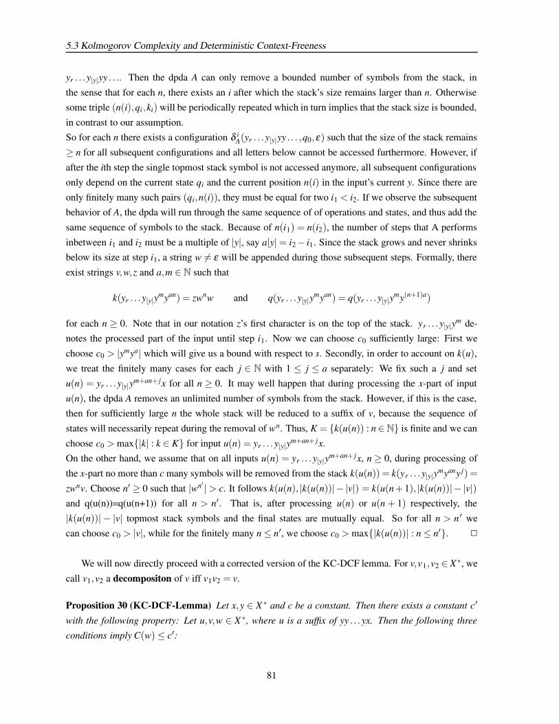
5.3 Kolmogorov Complexity and Deterministic Context-Freeness
yr . . .y|y|yy . . .. Then the dpda A can only remove a bounded number of symbols from the stack, in
the sense that for each n, there exists an i after which the stack’s size remains larger than n. Otherwisesome triple (n(i),qi,ki) will be periodically repeated which in turn implies that the stack size is bounded,
in contrast to our assumption.So for each n there exists a configuration δ i
A(yr . . .y|y|yy . . . ,q0,ε) such that the size of the stack remains
≥ n for all subsequent configurations and all letters below cannot be accessed furthermore. However, if
after the ith step the single topmost stack symbol is not accessed anymore, all subsequent configurationsonly depend on the current state qi and the current position n(i) in the input’s current y. Since there are
only finitely many such pairs (qi,n(i)), they must be equal for two i1 < i2. If we observe the subsequentbehavior of A, the dpda will run through the same sequence of of operations and states, and thus add the
same sequence of symbols to the stack. Because of n(i1) = n(i2), the number of steps that A performs
inbetween i1 and i2 must be a multiple of |y|, say a|y|= i2− i1. Since the stack grows and never shrinksbelow its size at step i1, a string w 6= ε will be appended during those subsequent steps. Formally, there
exist strings v,w,z and a,m ∈ N such that
k(yr . . .y|y|ymyan) = zwnw and q(yr . . .y|y|y
myan) = q(yr . . .y|y|ymy(n+1)a)
for each n ≥ 0. Note that in our notation z’s first character is on the top of the stack. yr . . .y|y|ym de-notes the processed part of the input until step i1. Now we can choose c0 sufficiently large: First we
choose c0 > |ymya| which will give us a bound with respect to s. Secondly, in order to account on k(u),
we treat the finitely many cases for each j ∈ N with 1 ≤ j ≤ a separately: We fix such a j and setu(n) = yr . . .y|y|ym+an+ jx for all n ≥ 0. It may well happen that during processing the x-part of input
u(n), the dpda A removes an unlimited number of symbols from the stack. However, if this is the case,then for sufficiently large n the whole stack will be reduced to a suffix of v, because the sequence of
states will necessarily repeat during the removal of wn. Thus, K = k(u(n)) : n ∈N is finite and we can
choose c0 >max|k| : k ∈ K for input u(n) = yr . . .y|y|ym+an+ jx.On the other hand, we assume that on all inputs u(n) = yr . . .y|y|ym+an+ jx, n ≥ 0, during processing of
the x-part no more than c many symbols will be removed from the stack k(u(n)) = k(yr . . .y|y|ymyany j) =
zwnv. Choose n′ ≥ 0 such that |wn′ |> c. It follows k(u(n), |k(u(n))|− |v|) = k(u(n + 1), |k(u(n))|− |v|)and q(u(n))=q(u(n+1)) for all n > n′. That is, after processing u(n) or u(n + 1) respectively, the
|k(u(n))| − |v| topmost stack symbols and the final states are mutually equal. So for all n > n ′ wecan choose c0 > |v|, while for the finitely many n≤ n′, we choose c0 >max|k(u(n))| : n≤ n′. 2
We will now directly proceed with a corrected version of the KC-DCF lemma. For v,v1,v2 ∈ X∗, we
call v1,v2 a decompositon of v iff v1v2 = v.
Proposition 30 (KC-DCF-Lemma) Let x,y ∈ X ∗ and c be a constant. Then there exists a constant c′
with the following property: Let u,v,w ∈ X ∗, where u is a suffix of yy . . . yx. Then the following three
conditions imply C(w)≤ c′:
81

Results from Formal Language Theory
(i) C(v′′|k$q) ≤ c, for all decompositions v′v′′ = v. Here, k,q is an arbitrary pair of a stack and a
state which, on processing v′′, induces the same behavior of A as the pair k(uv′),q(uv′);
(ii) C(w|k(uv)$q(uv)) ≤ c;
(iii) C(v)≥ 2 · lg(lg(|u|)).
In (i), same behavior of A for k,u and k(uv′),q(uv′) means the same sequence of states and operations.Formally: Let pr12(w,q,k) := (w,q) be the function that takes a configuration of A and forgets the stack.
Then all we assume from k,q is:
∀i≥ 0.pr12(δ iA(v′′,q,k)) = pr12(δ i
A(v′′,q(uv′),k(uv′))) .
PROOF: of the KC-DCF lemma: Let c0 be the constant from Proposition 29 and w be fixed. We distin-
guish two cases:
Case 1: Assume that for all but finitely many pairs (u,v) which satisfy (i)-(iii), the size of the stack
shrinks below c0 during processing the v-part on input uv. Then for each such pair a step i exists with
δ iA((v,q(u),k(u)) = (v′′,q,k) and |k| ≤m ,
where v = v′v′′ for some v′ and m≥ c0 and where m bounds the stack size for the finitely many remain-
ing pairs (u,v). Because of (i) we can reconstruct v′′ with only c many additional symbols, assuming a
description of q and k. Because |k| ≤ m, this can be done with finitely many symbols.Knowing v′′ and q,k we can reconstruct q(uv′v′′) = q(uv) and k(uv′v′′) = k(uv) by observing A on input
v′′, starting with q(uv′),k(uv′). Because of (ii) only c many further symbols will suffice to reconstruct
w. Hence C(w) is bounded by a sufficiently large constant c′.
Case 2: Now we show that case 1 always holds. Assume for the contrary, that for infinitely manypairs (u,v)
∀i≥ 0. δ iA((v,q(u),k(u)) = (v′′,q,k) ⇒ |k|> c0. (5.4)
holds and then derive a contradiction.For each u there exist only finitely many candidates v which satisfy (i). This is easy to see since
in (i), setting k = k(u), q = q(u), and v′ = ε suffices to show that for any given u, the description size
of all possible v is bounded. So if we assume there are infinitely many pairs satisfying (5.4), then wecan choose arbitrarily long u. Using Proposition 27 we choose |u| large enough such that there exists a
number r ∈ N with lg(r) > |u| andC(r)< lg(lg(|u|)) .
Using Proposition 29 we can find s≤ c0 such that the suffix u′ of length |u′|= r+s from yy . . . yx satisfies
q(u) = q(u′) and k(u, |k(u)|− c0) = k(u′, |k(u)|− c0) . (5.5)
82

5.3 Kolmogorov Complexity and Deterministic Context-Freeness
Because s is bounded we have C(u′)≤C(r) + O(1). For sufficiently large u we get
C(u′)< lg(lg(|u|)) . (5.6)
From the formulas (5.4) and (5.5)
∀i≥ 0. pr12(δ iA((v,q(u),k(u′))) = pr12(δ i
A((v,q(u),k(u))))
follows. Now (i) implies that v can be constructed when u′ is known: We let A work on input u′ until
q(u′) = q(u) and k(u′) = k(u). Then we use (i) and reconstruct v with c many additional symbols.Putting it all together we get
C(v) ≤ C(u′) + O(1)
≤ lg(lg(|u|)) + O(1) ,
where in the last step inequality (5.6) is used. This contradicts (iii). 2
Since the KC-DCF Lemma itself is difficult to apply, we also give the corresponding correctedformulation of its corollary (see [LiVi95]): We say that a program p decides L1 for L2, if on input
u ∈ L2 the program p terminates and decides u ∈ L1 correctly.
Corollary 31 Let L ⊆ X ∗ be a deterministic context-free language, x,y ∈ X ∗, and let c be a constant.
Then there exists a constant c′ with the following property: If u,v,w ∈ X ∗, where u is suffix of . . .yyx,
then the following three conditions imply C(w)≤ c′:
(i) C(v′′|puv′) ≤ c for all decompositions v′v′′ = v and for all programs puv′ that decide (uv′)−1L for
prefixv′′;
(ii) C(w|puv)≤ c for all programs puv that list (uv)−1L in lexicographic order;
(iii) C(v)≥ 2 · lg(lg(|u|))
PROOF: Let A be a dpda that recognizes L. If L = /0 or L = X ∗ nothing has to be shown. Otherwise
the KC-DCF lemma 30 holds and we can show that under the given assumptions, (i) and (ii) from thecorollary imply (i) and (ii) from the KC-DCF Lemma (proposition 30):
Asssume that, under the given premises, u,v satisfy (i) from the corollary. Let v ′v′′ = v, and let k,q bethe required additional information from condition (i) from the KC-DCF lemma. Now, if by using only
finitely many additional symbols we can construct a program puv′ that decides (uv′)−1L for prefixv′′,then the bound in condition (i) from the corollary induces the bound in condition (i) from the KC-DCFlemma. This construction of puv′ can be obtained by observing the dpda A on input v′′ when starting
with state q and stack k.
83

Results from Formal Language Theory
With a similar argument, (ii) from above implies condition (ii) from the KC-DCF lemma. 2
Though the original KC-DCF lemma and its corollary have been weakened in order to make them
correct, they still can be applied for several nondeterministic context-free languages without much ad-ditional effort. We give two examples taken from [LiVi95]:
Example 3 The set of palindroms L = x ∈ X ∗ : x = x−1 is not deterministic context-free.
PROOF: Set y = 0, x = 1, u = 0n1, and v = 0n. For an incompressible n we have
C(v) + O(1) = C(n)≥ lg(n) = lg(|u|−1),
implying (iii) of the corollary for sufficiently large n. Let v′v′′ = v, then v′′ is the lexicographically firststring in (uv′)−1L. Since all v are all 0, (i) is also satisfied. The lexicographically first string in (uv)−1L
starting with 1 is 10n, hence w = 10n satisfies (ii). On the other hand
C(w) + O(1) = C(n)≥ lg(n),
hence L can not be deterministic context-free. 2
Example 4 L = xy ∈ 0,1∗ : |x| = |y|,y contains at least one 1 is not deterministic context-free.
PROOF: Set y = 0, x = 1, u = 0n1, with |u| is even, and v = 0n+1. For incompressible n we have
C(v) + O(1) = C(n)≥ lg(n) = lg(|u|−1),
thus implying (iii) of the corollary for sufficiently large n. Let v′v′′ = v. We only need one bit to code
the information whether |v′| is even or odd. If |v′| is even (odd), then v′′ is the shortest string of even(odd) length which is all 0 and not belongs to (uv′)−1L. This shows that also (i) is satisfied. The
lexicographically first string which does not belong to (uv)−1L and starts with 1 is 102n+3. So withw = 102n+3, condition (ii) is satisfied, too. On the other hand we have
C(w) + O(1) = C(n)≥ lg(n),
hence L cannot be deterministic context-free. 2
5.4 Related Work
We do not know whether the connection between permutations and the context-free membership prob-
lem has been pointed out in a similar way before, other NP-complete problems related to formal lan-guages are listed in [GaJo 79]. It seems interesting to study the permutation operator further by exploring
other language classes or by imposing other restrictions on the functions f and g.
84
5.4 Related Work
The fact that associativity of the CYK-product and regular languages are related is implicit in many
discussions of parsing algorithms, see for instance the section on Earley parsing in [Har 78]. However,we do not know any previous generalization to idempotent semirings. For using semirings in order to
model language restrictions, one might be interested in consulting the book [KuSa 85] by W. Kuich andA. Salomaa, which is an extensive monograph on semirings in connection with formal language theory.
The KC-DCF lemma was first stated by M. Li and P. Vitányi, see [LiVi95]. A shortened proof of our
version of the lemma can be found in [Gli 03].
85


Chapter 6
Valiant Parsing
In this chapter we turn to context-free semiring parsing. During the past decade, context-free semiring
parsing has spawned new interest into parsing. Applications can be found in the fields of speech recog-nition, description of second order structures in computational biology, and for modelling recursive
combinatorial objects. The context-free semiring-parsing problem is, for a given semiring-valuedcontext-free grammar P = (X ,V, p,S) and a word w ∈ X ∗, to compute L(P)(w). For the definitions of
semiring-valued grammars, see section 4.1. Throughout this chapter, we will assume that P is in Chom-
sky normalform. If the underlying semiring is the boolean semiring, then semiring parsing is equal toplain context-free word recognition.
Context-free parsing is complicated by the following fact: For arbitrary context-free grammars P, the
CYK-product is — at least in general — not associative. Indeed, as we have seen in section 5.2, theclass of languages for which associativity holds is very restricted. Hence semiring parsing requires
to deal with non-associative multiplication. In [Val 74], Valiant has shown how transitive closure oftriangular n× n matrices can be reduced to matrix-multiplication, even in the case that multiplication
is non-associative. Valiant’s reduction is such that it does not consume much more time than matrix
multiplication, in the following sense: If matrix multiplication can be performed in time O(n2+ε) forsome ε > 0, then transitive closure is computable in time O(n2+ε), too. Subsequently, Valiant showed
in the same paper how plain context-free word recognition reduces to transitive matrix-closure, whilemaintaining the time bound O(n2+ε).
Valiant did not address semiring parsing, probably because it was not a central focus of researchback then. However, as we will see in section 6.1 of this chapter, his algorithm for transitive matrix
closure can be applied for context-free semiring parsing without any modification. Thus it opens thepossibility of context-free parsing in subcubic time for all semirings for which matrix multiplication can
be performed in subcubic time — either through exploiting hardware parallelism or, if applicable, by
algebraic techniques.On the downside, Valiant’s computation of transitive matrix closures via matrix multiplication involves
a complicated recursion which is difficult to keep track of, especially since one is not used to deal
87

Valiant Parsing
with the non-associative multiplication. In section 6.2 we give an alternative formulation of Valiant’s
reduction, which we hope is a more visual concept of the entire process. We build upon Rytter’s paperon context-free parsing via computing shortest paths on grids (see [Ryt 95]). Again, Rytter’s algorithm
does not consider semiring parsing. Adapting Rytter’s work to it is actually more complicated thanadapting Valiant’s transitive matrix closures, since the latter can be applied directly. We do this by using
endomorphisms on (additively written) monoids in order to define path values. Like non-associative
multiplication, endomorphisms distribute over sums, and allow to differentiate between right multipli-cation and left multiplication. This way we maintain enough information of the original problem in
order to show that Rytter’s approach is by no means weaker than Valiant’s, in the sense that it can itselfbe applied for computing transitive matrix closures. We hope that our treatment of Valiant’s reduction
will help programmers to implement subcubic semiring parsing in a modular way.
In section 6.3 we give some applications of Valiant’s reduction for context-free semiring parsing.
For some applications, the so-called bottom-up property of the resulting parser is crucial. What exactlywe mean by the term“bottom-up" is made more precise in section 6.2.
6.1 Semiring Parsing and Transitive Matrix Closures
Let M = (M,+,0) be a commutative monoid. Additionally, a binary operation × : M×M :→ M isdefined, which distributes over +:
(i) (a + b)× c = (a× c) + (b× c),
(ii) c× (a + b) = (c×a) + (c×b), and
(iii) 0× c = c×0 = c
hold for all a,b,c ∈ M. It is not required that × is associative. Still, × is called a (non-associative)multiplication. Homomorphisms on M are only required to respect addition + and may ignore ×.
First, we will introduce transitive closures of matrices over M. Then we proceed by showing howtransitive closures of strictly upper triangular matrices can be used for constructing a table parser for
context-free semiring parsing. Table parsing, briefly described, means to compute LPA(u) for a given
grammar P = (X ,V, p,S) and for each A ∈V and each infix u of a given input word w of length n. As a
result of our reduction, an upper time bound of O(2n+ε) with ε > 0 for n×n matrix multiplication over
the underlying semiring also holds for semiring parsing for the given grammar P.
Let (di j),(ei j) two n× n matrices with indices 1 ≤ i, j ≤ n and with entries in M. Their product isdefined as usually as
(d× e)i j := ∑1≤k≤n
dik× ek j .
88
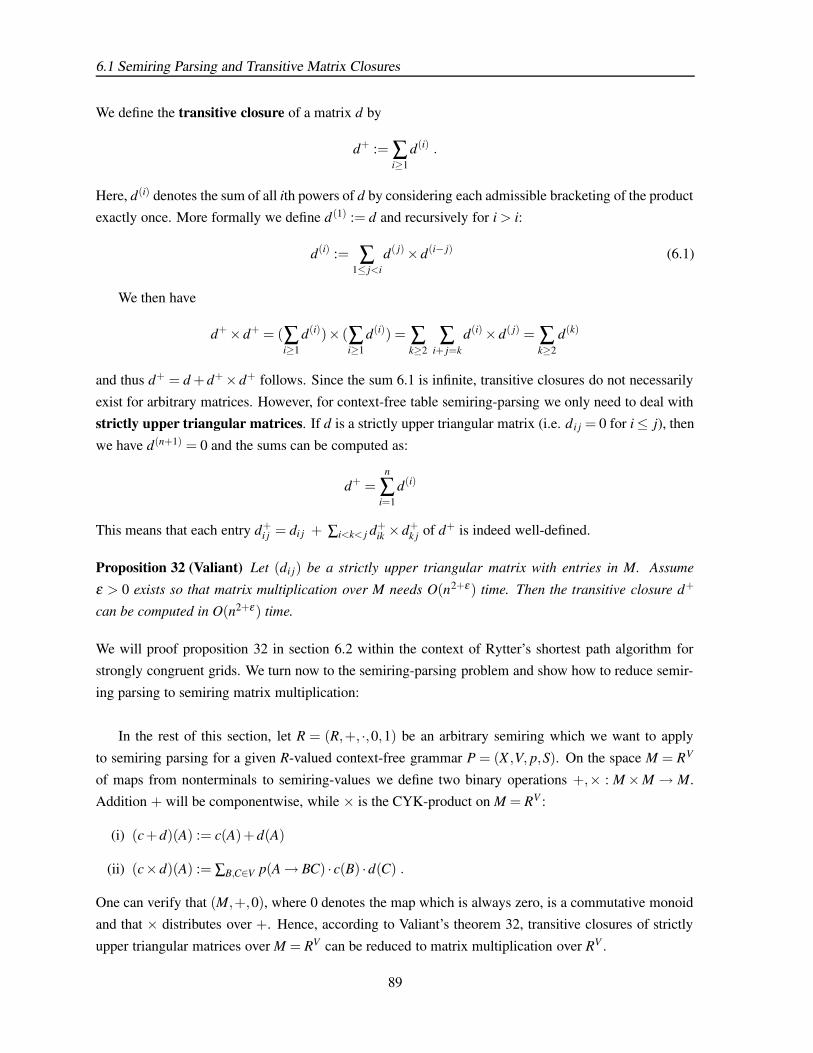
6.1 Semiring Parsing and Transitive Matrix Closures
We define the transitive closure of a matrix d by
d+ := ∑i≥1
d(i) .
Here, d(i) denotes the sum of all ith powers of d by considering each admissible bracketing of the productexactly once. More formally we define d (1) := d and recursively for i> i:
d(i) := ∑1≤ j<i
d( j)×d(i− j) (6.1)
We then have
d+×d+ = (∑i≥1
d(i))× (∑i≥1
d(i)) = ∑k≥2
∑i+ j=k
d(i)×d( j) = ∑k≥2
d(k)
and thus d+ = d + d+×d+ follows. Since the sum 6.1 is infinite, transitive closures do not necessarily
exist for arbitrary matrices. However, for context-free table semiring-parsing we only need to deal withstrictly upper triangular matrices. If d is a strictly upper triangular matrix (i.e. d i j = 0 for i≤ j), then
we have d(n+1) = 0 and the sums can be computed as:
d+ =n
∑i=1
d(i)
This means that each entry d+i j = di j + ∑i<k< j d+
ik ×d+k j of d+ is indeed well-defined.
Proposition 32 (Valiant) Let (di j) be a strictly upper triangular matrix with entries in M. Assume
ε > 0 exists so that matrix multiplication over M needs O(n2+ε) time. Then the transitive closure d+
can be computed in O(n2+ε) time.
We will proof proposition 32 in section 6.2 within the context of Rytter’s shortest path algorithm forstrongly congruent grids. We turn now to the semiring-parsing problem and show how to reduce semir-
ing parsing to semiring matrix multiplication:
In the rest of this section, let R = (R,+, ·,0,1) be an arbitrary semiring which we want to apply
to semiring parsing for a given R-valued context-free grammar P = (X ,V, p,S). On the space M = RV
of maps from nonterminals to semiring-values we define two binary operations +,× : M×M → M.Addition + will be componentwise, while × is the CYK-product on M = RV :
(i) (c + d)(A) := c(A) + d(A)
(ii) (c×d)(A) := ∑B,C∈V p(A→ BC) · c(B) ·d(C) .
One can verify that (M,+,0), where 0 denotes the map which is always zero, is a commutative monoidand that × distributes over +. Hence, according to Valiant’s theorem 32, transitive closures of strictly
upper triangular matrices over M = RV can be reduced to matrix multiplication over RV .
89
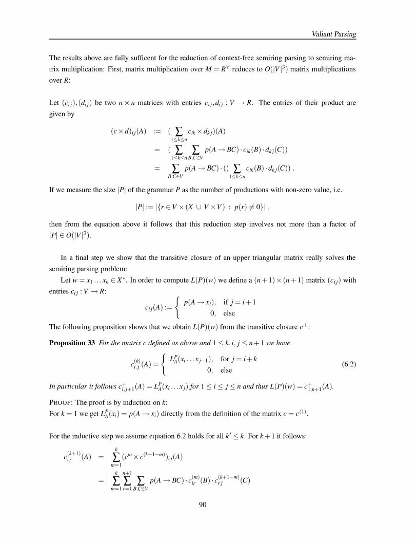
Valiant Parsing
The results above are fully sufficent for the reduction of context-free semiring parsing to semiring ma-
trix multiplication: First, matrix multiplication over M = RV reduces to O(|V |3) matrix multiplicationsover R:
Let (ci j),(di j) be two n× n matrices with entries ci j,di j : V → R. The entries of their product are
given by
(c×d)i j(A) := ( ∑1≤k≤n
cik×dk j)(A)
= ( ∑1≤k≤n
∑B,C∈V
p(A→ BC) · cik(B) ·dk j(C))
= ∑B,C∈V
p(A→ BC) · (( ∑1≤k≤n
cik(B) ·dk j(C)) .
If we measure the size |P| of the grammar P as the number of productions with non-zero value, i.e.
|P| := |r ∈V × (X ∪ V ×V ) : p(r) 6= 0| ,
then from the equation above it follows that this reduction step involves not more than a factor of|P| ∈ O(|V |3).
In a final step we show that the transitive closure of an upper triangular matrix really solves the
semiring parsing problem:
Let w = x1 . . .xn ∈ X∗. In order to compute L(P)(w) we define a (n + 1)× (n + 1) matrix (ci j) withentries ci j : V → R:
ci j(A) :=
p(A→ xi), if j = i + 1
0, else
The following proposition shows that we obtain L(P)(w) from the transitive closure c+:
Proposition 33 For the matrix c defined as above and 1≤ k, i, j ≤ n + 1 we have
c(k)i, j (A) =
LP
A(xi . . .x j−1), for j = i + k
0, else(6.2)
In particular it follows c+i, j+1(A) = LP
A(xi . . .x j) for 1≤ i≤ j ≤ n and thus L(P)(w) = c+1,n+1(A).
PROOF: The proof is by induction on k:For k = 1 we get LP
A(xi) = p(A→ xi) directly from the definition of the matrix c = c(1).
For the inductive step we assume equation 6.2 holds for all k ′ ≤ k. For k + 1 it follows:
c(k+1)i j (A) =
k
∑m=1
(cm× c(k+1−m))i j(A)
=k
∑m=1
n+1
∑r=1
∑B,C∈V
p(A→ BC) · c(m)ir (B) · c(k+1−m)
r j (C)
90

6.2 Transitive Closure via Shortest Paths
(by the inductive hypotheses: c(m)ir (B) =
0, if r 6= i + m
LPB(xi . . .xi+m−1), else
)
=k
∑m=1
∑B,C∈V
p(A→ BC) ·LPB(xi . . .xi+m−1) · c(k+1−m)
i+m, j (C)
Now, by the inductive hypothesis for c(k+1−m)i+m, j (C), i.e.
c(k+1−m)i+m, j (C) =
LP
C(xi+m . . .x j−1), if j = i + k + 1
0, else
it follows c(k+1)i j = 0 for j 6= i + k + 1 while for j = i + k + 1 we get
c(k+1)i j (A) =
k
∑m=1
∑B,C∈V
p(A→ BC) ·LPB(xi . . .xi+m−1) ·LP
C(xi+m . . .x j−1)
=j−1
∑m=i
∑B,C∈V
p(A→ BC) ·LPB(xi . . .xm−1) ·LP
C(xm . . .x j−1)
= LPA(xi . . .x j−1)
since P is in Chomsky normalform. 2
By applying the reductions above, we get the following bounds for semiring-parsing:
Proposition 34 Let R be a semiring for which n×n matrix multiplication needs O(n2+ε) time for some
ε > 0. Let P = (X ,V, p,S) be a R-valued context-free grammar in Chomsky normalform and w ∈ X n.
Then L(P)(w) can be computed in O(n2+ε |P|) time. 2
6.2 Transitive Closure via Shortest Paths
6.2.1 Bottom-Up Properties
The results of the previous section together with Valiant’s reduction for transitive closure ensure that
we can, for all semirings, reduce the semiring parsing problem to semiring matrix multiplication. There
are two reasons why we want to re-examine Valiant’s reduction in the following section: The first oneis that Valiant’s original description of the reduction algorithm is not very visual to the reader. In the
past, other researchers have reformulated Valiant’s algorithm, see section 6.4. However, none of the au-thors, including Valiant, considered semiring parsing. In the context of the emerging interest in parsing
methods for semiring parsing, the question rose naturally how to investigate how well the alternative
approaches to Valiant’s reduction generalize. In this section we will show that Rytter’s approach cannotonly be generalized for context-free semiring parsing, but also for the more general problem of comput-
ing transitive closures of upper triangular matrices.
91
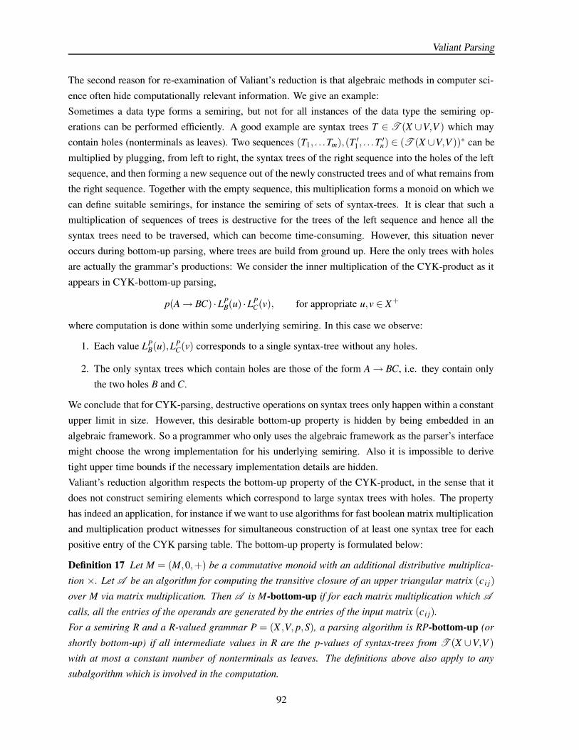
Valiant Parsing
The second reason for re-examination of Valiant’s reduction is that algebraic methods in computer sci-
ence often hide computationally relevant information. We give an example:Sometimes a data type forms a semiring, but not for all instances of the data type the semiring op-
erations can be performed efficiently. A good example are syntax trees T ∈ T (X ∪V,V ) which maycontain holes (nonterminals as leaves). Two sequences (T1, . . .Tm),(T ′1 , . . .T
′n) ∈ (T (X ∪V,V ))∗ can be
multiplied by plugging, from left to right, the syntax trees of the right sequence into the holes of the left
sequence, and then forming a new sequence out of the newly constructed trees and of what remains fromthe right sequence. Together with the empty sequence, this multiplication forms a monoid on which we
can define suitable semirings, for instance the semiring of sets of syntax-trees. It is clear that such amultiplication of sequences of trees is destructive for the trees of the left sequence and hence all the
syntax trees need to be traversed, which can become time-consuming. However, this situation never
occurs during bottom-up parsing, where trees are build from ground up. Here the only trees with holesare actually the grammar’s productions: We consider the inner multiplication of the CYK-product as it
appears in CYK-bottom-up parsing,
p(A→ BC) ·LPB(u) ·LP
C(v), for appropriate u,v ∈ X +
where computation is done within some underlying semiring. In this case we observe:
1. Each value LPB(u),LP
C(v) corresponds to a single syntax-tree without any holes.
2. The only syntax trees which contain holes are those of the form A→ BC, i.e. they contain only
the two holes B and C.
We conclude that for CYK-parsing, destructive operations on syntax trees only happen within a constant
upper limit in size. However, this desirable bottom-up property is hidden by being embedded in an
algebraic framework. So a programmer who only uses the algebraic framework as the parser’s interfacemight choose the wrong implementation for his underlying semiring. Also it is impossible to derive
tight upper time bounds if the necessary implementation details are hidden.Valiant’s reduction algorithm respects the bottom-up property of the CYK-product, in the sense that it
does not construct semiring elements which correspond to large syntax trees with holes. The property
has indeed an application, for instance if we want to use algorithms for fast boolean matrix multiplicationand multiplication product witnesses for simultaneous construction of at least one syntax tree for each
positive entry of the CYK parsing table. The bottom-up property is formulated below:
Definition 17 Let M = (M,0,+) be a commutative monoid with an additional distributive multiplica-
tion ×. Let A be an algorithm for computing the transitive closure of an upper triangular matrix (c i j)
over M via matrix multiplication. Then A is M-bottom-up if for each matrix multiplication which A
calls, all the entries of the operands are generated by the entries of the input matrix (c i j).
For a semiring R and a R-valued grammar P = (X ,V, p,S), a parsing algorithm is RP-bottom-up (or
shortly bottom-up) if all intermediate values in R are the p-values of syntax-trees from T (X ∪V,V )
with at most a constant number of nonterminals as leaves. The definitions above also apply to any
subalgorithm which is involved in the computation.
92

6.2 Transitive Closure via Shortest Paths
The bottom-up property of a transitive-closure reduction which works for arbitrary M is very natural:
Without any knowledge about M, where — if not from the input itself — should intermediate values begenerated from?
The bottom-up property of a semiring-parser is more restrictive. Indeed there exist many parsing algo-rithms, like Early parsing, which are not bottom-up. However, the construction of M = RV and the initial
matrix (ci j) in the previous section ensure that each subsequent M-bottom-up Valiant reduction results
in a bottom-up parser, provided that matrix multiplication is M-bottom-up. This observation followsdirectly from the definition of the CYK-product on M = RV and the discussion above.
6.2.2 Strongly Congruent Grids and Shortest Paths
We will now give a proof for Valiant’s reduction in terms of a suitable algorithm. Valiant himself al-ready gave a proof in his paper [Val 74], but we will use ideas from Rytter’s parsing algorithm (see
[Ryt 95]). Since Rytter formulated his algorithm for plain context-free parsing, we need a considerable
amount of generalizations in order to show that Rytter’s algorithm is also suitable to compute transitiveclosures of triangular matrices over arbitrary M. The advantage of Rytter’s approach lies in Valiant’s
reduction being formulated in terms of a shortest path problem. The graphs which we consider will betwo-dimensional grids. This is more intuitive than working with non-associative multiplication, which
we will get rid of by replacing it by endomorphisms.
Let (M,+,0) be a commutative monoid and × be a distributive multiplication. The distributive laws
ensure that for each a ∈ M, left-multiplication x 7→ ax and right-multiplication x 7→ xa are endomor-
phisms (i.e. homorphisms from M onto itself). For the shortest path problem on strongly congruentgrids, we replace × by two monoids of endomorhisms: We define H1 and H2 to be the sets of all left-
and right-multiplications on M respectively. With · as the concatenation of maps and 1 being the identitymap, (H1, ·,1) and (H2, ·,1) are both monoids of M-endomorphisms. Given a set of M-endomorphisms
H and two n×n matrices (hi j),(ci j) with hi j ∈ H and ci j ∈M, we define their matrix product as
(h× c)i j =n
∑k=1
hik(ck j) . (6.3)
Definition 18 A n× n grid is a directed graph G = (N,E) with nodes N = 1..n×1..n and edges
E = E1∪E2 with E1 = ((i, j),(i, j + k)) : k > 0 and E2 = ((i + k, j),(i, j)) : k > 0. For a commu-
tative monoid M = (M,+,0) and two sets H1,H2 of M-endomorphisms, a strongly congruent grid is a
grid G = (N,E) with a node labelling K : N→M and an edge labelling h : E→ H1∪H2 such that:
(i) h(Ei)⊆ Hi for i = 1,2.
(ii) h((i, j),(i + k, j)) = h((i, j′),(i + k, j′)) for all 1≤ i, j, j′,k ≤ n with i + k≤ n.
(iii) h((i, j),(i, j + k)) = h((i′, j),(i′, j + k)) for all 1≤ i, i′, j,k ≤ n with j + k ≤ n.
93
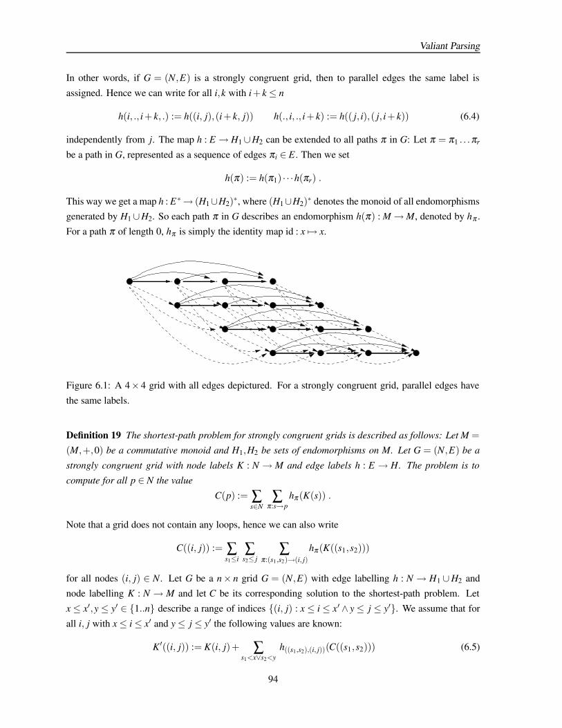
Valiant Parsing
In other words, if G = (N,E) is a strongly congruent grid, then to parallel edges the same label is
assigned. Hence we can write for all i,k with i + k≤ n
h(i, ., i + k, .) := h((i, j),(i + k, j)) h(., i, ., i + k) := h(( j, i),( j, i + k)) (6.4)
independently from j. The map h : E → H1∪H2 can be extended to all paths π in G: Let π = π1 . . .πr
be a path in G, represented as a sequence of edges πi ∈ E . Then we set
h(π) := h(π1) · · ·h(πr) .
This way we get a map h : E∗→ (H1∪H2)∗, where (H1∪H2)∗ denotes the monoid of all endomorphismsgenerated by H1∪H2. So each path π in G describes an endomorphism h(π) : M→M, denoted by hπ .
For a path π of length 0, hπ is simply the identity map id : x 7→ x.
Figure 6.1: A 4× 4 grid with all edges depictured. For a strongly congruent grid, parallel edges have
the same labels.
Definition 19 The shortest-path problem for strongly congruent grids is described as follows: Let M =
(M,+,0) be a commutative monoid and H1,H2 be sets of endomorphisms on M. Let G = (N,E) be a
strongly congruent grid with node labels K : N → M and edge labels h : E → H. The problem is to
compute for all p ∈ N the value
C(p) := ∑s∈N
∑π:s→p
hπ (K(s)) .
Note that a grid does not contain any loops, hence we can also write
C((i, j)) := ∑s1≤i
∑s2≤ j
∑π:(s1,s2)→(i, j)
hπ (K((s1,s2)))
for all nodes (i, j) ∈ N. Let G be a n× n grid G = (N,E) with edge labelling h : N → H1 ∪H2 andnode labelling K : N → M and let C be its corresponding solution to the shortest-path problem. Let
x ≤ x′,y ≤ y′ ∈ 1..n describe a range of indices (i, j) : x ≤ i ≤ x′ ∧ y≤ j ≤ y′. We assume that for
all i, j with x≤ i≤ x′ and y≤ j ≤ y′ the following values are known:
K′((i, j)) := K(i, j) + ∑s1<x∨s2<y
h((s1,s2),(i, j))(C((s1,s2))) (6.5)
94

6.2 Transitive Closure via Shortest Paths
Note that we do not use the C(i, j)-values in the range x ≤ i ≤ x′ and y ≤ j ≤ y′. Instead, we compute
the shortest-path values C′(i, j) of the subgrid induced by the nodes (i, j) with x≤ i≤ x′ and y≤ j ≤ y′,i.e.
C′((i, j)) := ∑x≤s1≤iy≤s2≤ j
∑π:(s1,s2)→(i, j)
hπ (K′((s1,s2))) .
We find that for x≤ i≤ x′ and y≤ j ≤ y′, the values C′((i, j)) and C((i, j)) are equal:
C′((i, j)) = ∑x≤s1≤iy≤s2≤ j
∑π:(s1,s2)→(i, j)
hπ
K(s1,s2) + ∑
s′1<x∨s′2<yh((s′1,s
′2),(s1,s2))(C((s′1,s
′2)))
= ∑x≤s1≤iy≤s2≤ j
∑π:(s1,s2)→(i, j)
hπ (K(s1,s2))
+ ∑x≤s1≤iy≤s2≤ j
∑π:(s1,s2)→(i, j)
hπ
∑
s′1<x∨s′2<yh((s′1,s
′2),(s1,s2))
∑
s′′1≤s′1s′′2≤s′2
∑π ′:(s′′1 ,s
′′2)→(s1,s2)
hπ ′(K(s′′1 ,s′′2)))
= ∑x≤s1≤iy≤s2≤ j
∑π:(s1,s2)→(i, j)
hπ (K(s1,s2))
+ ∑s′1<x∨s′2<y
∑s′1<x∨s′2<y
∑s′′1≤s′1s′′2≤s′2
∑π:(s1 ,s2)→(i, j)
π′:(s′′1 ,s′′2 )→(s′1 ,s
′2)
hπ ′·((s′1,s′2)(s1,s2))·π(K(s′′1 ,s
′′2)))
= ∑x≤s1≤iy≤s2≤ j
∑π:(s1,s2)→(i, j)
hπ (K(s1,s2)) + ∑s1<x∨s2<y
∑π:(s1,s2)→(i, j)
hπ(K(s1,s2))
= ∑s1≤is2≤ j
∑π:(s1,s2)→(i, j)
hπ (K(s1,s2)) = C((i, j))
Assuming the shortest-path values C((i, j)) for x ≤ i≤ x′ and y ≤ j ≤ y′ are the only missing ones, we
can compute them from the values K ′((i, j)) (equation 6.5) and the solution of the shortest path problemfor the corresponding subgrid. This suggests a recursive splitting of a grid for solving the shortest path
problem. All we have to do is to maintain equation 6.5 for the subgrid in question. We will see belowhow this can be done by matrix multiplications of the form as defined in equation 6.3. For a better
understanding, please note that equation 6.3 defines an application of a matrix of endomorphisms to a
matrix of monoid values.
Proposition 35 (Generalized Rytter Reduction) Let G be a n × n strongly congruent grid with
node labels in a commutative monoid M and edge labels in H1,H2, where H1, H2 are sets of M-
endomorphisms. Then the shortest-path problem for G can be reduced to multiplication of matrices
as defined in equation 6.3, where entries of the first operand matrix are either all from H1 or all from
H2, and the entries of the second operand matrix are all from M. For the reduction, the following time
bound holds: If those matrix multiplications for n× n matrices can be computed in time O(n2+ε) for
some ε > 0, then the shortest-path problem for G can be computed in time O(n2+ε).The reduction is
M-bottom-up.
95

Valiant Parsing
PROOF: Let G = (N,E) be a grid and M,H1,H2 be given as described in the precondition of the propo-
sition. Let K : N→M and h : E → H1∪H2 be labellings such that G,K,h is a strongly congruent gridand let C : N→M be its solution for the shortest-path problem. We want to describe an algorithm which
computes all values C(i, j), for (i, j) ∈N by using matrix-multiplication of the form of equation 6.3. Forthe sake of simplicity we assume that G is a n× n grid where n is a power of 2. This is not a loss of
generality since we can always solve the shortest path problem by enlarging the grid until its size is a
power of 2. The extra costs for solving the shortest-path problem on the larger grid are then negligible.For n ≤ 1 we do not need to to anything. For all other n ≤ 2 we proceed by recursion. We can assume
that G = (N,E) is a 2n×2n grid and that we can already solve the shortest-path problem for n×n gridsby recursive calls to our algorithm. We define the following sets:
N1 := (i, j) ∈ N : i≤ n ∧ j ≤ n
N2 := (i, j) ∈ N : i≤ n ∧ n < j ≤ 2n
N3 := (i, j) ∈ N : n < i≤ 2n ∧ j ≤ n
N4 := (i, j) ∈ N : n < i≤ 2n ∧ n < j ≤ 2n
The idea is to compute, in the order listed here, the values C(i, j): first for all (i, j) ∈ N1, then for all
(i, j) ∈ N2, for all (i, j) ∈ N3, and finally for all (i, j) ∈ N4.For (i, j) ∈ N1, the values C(i, j) coincide with the values of the shortest-path problem for the subgrid
induced by N1. Hence we can compute them by recursively calling our algorithm for the smaller n×n
subgrid.For (i, j) ∈ N2, we proceed as follows: First, for all such (i, j) ∈ N2, we compute
K′((i, j)) := K((i, j)) +n
∑k=1
h(.,k, ., j)(C((i,k))) .
Note that K ′((i, j)) can be computed for all (i, j) ∈ N2 simultaneously by a matrix multiplication of
the form in equation 6.3 and then adding the original values K((i, j)). By setting x = 1,x ′ = n,y =
n + 1,y′ = 2n, K ′ satisfies equation 6.5. We can now obtain the values C((i, j)) for (i, j) ∈ N2 by
recursively computing the shortest-path values for the subgrid induced by N2 together with the new
labels K ′.For (i, j) ∈ N3, we proceed in a similar way: For all such (i, j) ∈ N3, we compute
K′((i, j)) := K((i, j)) +n
∑k=1
h(k, ., i, .)(C((k, j)))
by using a single matrix multiplication. Again, we obtain the values C((i, j)) for (i, j) ∈ N3 by recur-sively computing the shortest-path values for the subgrid induced by N3 and node labels K ′.
Finally, for (i, j) ∈ N4 we compute
K′((i, j)) := K((i, j)) +n
∑k=1
h(.,k, ., j)(C((i,k))) +n
∑k=1
h(k, ., i, .)(C((k, j)))
96
6.2 Transitive Closure via Shortest Paths
by using two matrix multiplications. A last recursive call of the algorithm will then compute the missing
values C((i, j)) for (i, j) ∈ N4.
In each recursive step with a n×n grid as its input, the algorithm above requires exactly 4 n/2×n/2matrix multiplications of the form of equation 6.3. According to our assumptions, this takes O(n2+ε)
time for some ε > 0. Also in each recursive step, the algorithm calls itself four times, each time for a
subgrid of size n/2×n/2. The running time T (n) is therefore bounded by
T (n) = 4 ·O((n/2)2+ε ) + 4T(n/2)
while T (n) = O(1) for n = 1. This yields T (n) = O(n2+ε). Finally we conclude that the algorithm is M-
bottom-up by observing that all intermediate values in M are generated by the values of the algorithm’sinput grid. 2
Rytter formulated the boolean case of the shortest path problem for strongly congruent grids as amean to reduce plain context-free parsing to boolean matrix multiplication. Though the reduction is
much more visible, it does not generalize that easily to semiring parsing. We show that with our gen-eralizations, the more general transitive closure problem reduces to it. As discussed in section 6.1, this
will in turn allow semiring parsing.
Proposition 36 Let M = (M,+,0) be a commutative monoid and × be a binary multiplication which
distributes over +. Let H1,H2 be some sets of, respectively, left- and right-multiplications over M. If the
shortest-path problem for strongly congruent grids G with node labels in M and edge labels in H1,H2
can be solved in O(n2+ε) time for some ε > 0, then transitive matrix closures for upper triangular
matrices over M can be computed in O(n2+ε) time. The reduction is M-bottom-up.
Before we prove proposition 36, we note that now Valiant’s theorem 32 follows directly from the propo-sitions 35 and 36. Indeed, matrices of left-multiplications can be encoded as matrices over M, such that
equation 6.3 refers to a simple semiring matrix multiplication. The same holds for application matrices
over right-multiplications, with the only difference that the matrix of multipliers is multiplied to theright. We can also see that Valiant’s reduction is M-bottom-up.
PROOF: (of proposition 36)Let M = (M,+,0) be a commutative monoid and × be a distributive multiplication and H1, H2 be as
defined in the preconditions of the proposition. Let (di j) be a n×n strictly upper triangular matrix withentries in M. For the sake of simplicity, we assume that n is a power of 2. If not, we can append O(n)
zero rows and zero columns to d.
We show proposition 36 by induction. For n ≤ 1, nothing has to be done in order to compute the
transitive closure d+. In our inductive step, we assume the truth of proposition 36 for matrices of size
97

Valiant Parsing
n×n. So we continue with for 2n×2n matrices:
Let d be a 2n×2n matrix, n≥ 2, with entries in M. For indices i, j with 1≤ i, j≤ n∨n≤ i, j≤ 2n we
can compute the correct values d+i j recursively by computing the transitive closures of the corresponding
submatrices. What is left to compute are the missing values d+i j for 1≤ i< n∧n< j≤ 2n: For the n×n
grid G = (N,E) we define the following node labels K : N → M and edge labels h : E → H1 ∪H2 by
settingK((i, j)) := dn+1−i,n+ j for 1≤ i, j ≤ n,
and
h(k, ., i, .) := x 7→ d+n+1−i,n+1−k× x and h(k, ., j, .) := x 7→ x×d+
n+k,n+ j
for 1≤ k < i, j ≤ n, see equation 6.4. Our claim is now that the solution
C(p) := ∑s∈N
∑π:s→p
hπ (K(s))
of the shortest-path problem for the strongly congruent grid G with labels h,K yields the missing entriesof d+: It is
C(p) = d+n+1−i,n+ j
for all nodes p = (i, j) with 1≤ i, j ≤ n . We show this by induction on the difference j− i.
j = i = 1: Since in the n× n grid G there is only the path of length 0 from the node (1,1) to itself, weget
C((i, j)) = id(K((1,1))) = dn,n+1 = d+n,n+1 .
For the inductive step, we assume C((i, j)) = d+n+1−i,n+ j for 2≤ i+ j< r. We then conclude for i+ j = r:
C((i, j)) = K((i, j)) + ∑k<i
h(k, ., i, .)(C((k, j)) + ∑k< j
h(.,k, ., j)C((i,k))
= dn+1−i,n+ j + ∑k<i
d+n+1−i,n+1−k×d+
n+1−k,n+ j
+ ∑k< j
d+n+1−i,n+k×d+
n+k,n+ j
= dn+1−i,n+ j + ∑n+1−i<k<n+ j
d+n+1−i,k×d+
k,n+ j
= d+n+1−i,n+ j
The algorithm is M-bottom-up. This can be verified by inspection, i.e. one can see values from
M are never used which are not generated by the input values. Finally, after establishing correctnessof the algorithm, we derive the required time bounds: For a given n× n input matrix, n = 2k, in each
recursive step the algorithm calls itself twice for matrices of the size n/2× n/2, followed by a callto the shortest-path algorithm for a grid of size n/2× n/2. The time for constructing the grid G is
negligible. Under the assumption of the proposition our algorithm has an upper timebound T (n) which
satisfies T (n) = 2T (n/2) + O(n2+ε) for all n = 2k and T (1) = O(1). It follows that T itself satisfiesT (n) = O(n2+ε). 2
98

6.3 Applications
6.3 Applications
Only briefly we will mention some applications of Valiant parsing for some semirings for which matrix
multiplication can be computed in subcubic time. For a thorough discussion of semiring parsing, the
reader is referred to [Goo 98].
For the boolean semiring IB = (0,1,∨,∧,0,1) as the underlying semiring we are down to plain
context-free parsing for context-free grammars P = (X ,V,P,S). Boolean matrix-multiplication can be
embedded into matrix mutliplication over the integers, and known subcubic matrix multiplication algo-rithms involve only a modest growth of the size of numbers during computation. Hence Valiant parsing
can be used in order to construct a recognition matrix for an input string w ∈ X ∗ in subcubic time. The
recognition matrix represents in a certain way all possible parses, but an arbitrary syntax tree (if it exists)can be constructed in O(n) time.
In some applications it might be desirable to have one — or a finite number of — valid syntax trees foreach infix of the input string w. This is useful if the input is subject to change or for error analysis in
language processing. It turns out that Valiant parsing can simultaneously construct an arbitrary syntax-
tree for each infix of w and nonterminal A ∈ V . Our discussion tries to avoid technical details, whichwill actually involve to re-examine the entire algorithm again:
We start with the monoid T ∗ = (T (X ∪V,V )∗, ·,ε) of syntax trees which are allowed to contain
holes (nonterminals as leaves). As mentioned in section 6.2, for two sequences (T1, . . . ,Tm),(T ′1 , . . . ,T′
n)∈T ∗, their product is defined by plugging the trees T ′1, . . . ,T
′min(n′,r) from left to right into the r holes
of T1, . . . ,Tm. Their product is the resulting sequence concatenated with the remaining sequence
(T ′min(n′,r)+1, . . . ,T′
n). One can verify that T ∗ is indeed a monoid. Based on T ∗ we can define thesemiring (2T ∗
,∪, ·, /0, ·), where for two sets F,G⊆T ∗ we define
F ·G := (T1, . . . ,Tm) · (T ′1, . . . ,T′
n) : (T1, . . . ,Tm) ∈ F,(T ′1 , . . . ,T′
n) ∈G .
Using 2T ∗as the underlying semiring, Valiant’s algorithm will compute the set of all syntax trees for
each A ∈V and each infix of the input word w by using matrix multiplication over 2T ∗. This, however,
cannot be implemented in polynomial time since the number of possible syntax trees may grow expo-
nentially.1 If we are satisfied by obtaining only one syntax tree (if it exists) as a suitable representative
for the entire class of valid syntax tree from A ∈V to each infix u, we could naively identify all syntaxtrees with equal root and equal front. The resulting structure will still be a semiring. However, we
must be a bit more careful since the actual form of the representative is not a property of the underlying
semiring. The parsing algorithm might well mess up and yield a representative where root and front fit,but is not valid for the grammar P. In fact, we need to inspect the parsing algorithm in order to convince
ourselves that it does not mess up and produces invalid syntax trees. We omit the proof here. Anothersolution might be to either construct a more complicated semiring (which we doubt being possible), or
1At least not for “natural" representations of syntax trees. But in some way, the recognition matrix itself can be understoodas a proper representation of all possible syntax trees.
99

Valiant Parsing
to find a better interface than the semiring framework.
Given two n× n matrices (ci j),(di j) whichs entries are either a syntax tree or zero, it remains to showthat they can be multiplied in subcubic time. The task is to compute a product matrix (e i j) which
has a zero entry at ei j if and only if no k = 1..n with cik 6= 0 and dk j 6= 0 exists. Otherwhise one isallowed to choose some k with cik 6= 0 and dk j 6= 0 and combine the two syntax-trees cik and dk j in
order to form ei j . This can be achieved by using boolean matrix multiplication and the subsequent
computation of boolean matrix multiplication witnesses. For both, subcubic algorithms exists sincethe boolean-matrix-multiplication-witness problem actually reduces to boolean matrix multiplication (a
probabilistic algorithm can be found in [MoRa 95]). Also, since Valiant’s reduction yields a bottom-upparser, newly constructed syntax-trees can be build non-destructively.
Finally we mention the following semirings which allow subcubic parsing:
1. The semiring of natural numbers with addition and multiplication as usual. This allows to count
the number of syntax trees for a given input word w and for all its infixes and nonterminals A∈V ,similtaniously. Note that the numbers can grow exponential and hence the number of bits for their
representation grows lineary. If we do not need to obtain exact results for very large numbers, we
can either bound the maximum representable number, or work with approximations like floatingpoint numbers.
2. The semiring ([0..1],+, ·,0,1) which can represent probabilities of derivations.
6.4 Related Work
Valiant’s reduction involves a complicated recursion scheme. There have been many subsequent refor-
mulations of it inorder to make his result more accessible. See for instance the book [Har 78] and thepaper [Wal 84]. The idea of describing Valiant’s reduction in terms of a shortest-path problem is from
[Ryt 95]. Semiring parsing in general is treated in depth in the thesis [Goo 98]. The paper [Lee 02]
shows that plain context-free parsing (under very reasonable assumptions2) is at least as difficult asboolean matrix multiplication. It might be interesting to investigate how far the latter result extends to
general semiring parsing.
2Lee assumes that grammar size induces at most a linear factor in parsing time and that the parser produces informationabout the parsing process.
100
Appendix A
Definitions from Graph Theory
We recall, mostly in order to settle notation, some basic definitions of graph theory:
Definition 20 (directed and undirected graphs) A directed graph (or: digraph) G = (N,E) consists
of a finite set of nodes N and a set of edges E ⊆ N×N of ordered node-pairs. An undirected graphG = (N,E) has a finite set of nodes N and the set of edges is a set E ⊆ p,q : p 6= q ∈ E of unordered
node-pairs. In the undirected case we sometimes write (p,q) for some edge p,q ∈ E so that we
identify (p,q) and (q, p). For (p,q) ∈ E we then say that the nodes p,q are neighbours and that they
are joined by the edge e = (p,q). An edge of the form e = (p, p) is called a l¯oop.
Note that according to our definition, undirected graphs never contain any loops. This might be adefect if we want to go from a digraph to the underlying undirected graph by forgetting the directions
of the edges. However, we never use undirected graphs with loops in this thesis and by this way the
following definitions work conveniently for both, directed and undirected graphs:
Definition 21 (paths and cycles) Let G = (N,E) be a graph (directed or undirected). A graph G ′ =
(N ′,E ′) with N ′ ⊆N and E ′ ⊆ E is called a subgraph of G. Furthermore, G′ is an induced subgraph if
E ′= (p,q)∈E : p,q∈N ′. A path in G from p∈N to q∈N is a sequence of nodes π = π0, . . . ,πk ∈N∗
such that (πi−1,πi) ∈ E for all i = 1..k, and π0 = p,πk = q. The length of π is denoted by |π| := k.
The fact that a path π starts in node p and ends in q is denoted by π : p→G q, where the subscript
G is sometimes omitted in the case that the context is clear. An edge e ∈ E is traversed by a path
π = π0, . . . ,πk if e = (πi−1,πi) for some i = 1..k. For a graph G the set of all paths contained in G is
denoted by Π(G). A path is simple if it traverses no edge more than once. G is connected when there
always exists a path in G between arbitrary nodes p,q ∈ N. The path π = π0, . . . ,πk is closed when
π0 = πk. Furthermore, a closed path π = π0, . . . ,πk−1,π0 in a directed graph G is a cycle if pi 6= p j
for all 0 ≤ i < j < k. In the undirected case we additionally demand that |π| 6= 2, thus a cycle can
be identified (up to rotation of nodes) with a connected subgraph where each node has exactly two
neighbors. A graph (directed or undirected) is acyclic if it contains no cycles.
101

Definitions from Graph Theory
Definition 22 (edge labeling) For a graph G = (N,E) and a set R, an edge labeling with values in R
is a map X : E→ R. In the case that R = (R, ·,1) is a monoid, we extend X to a mapping X : Π(G)→ R
by
X(π) := X(π0,π1) · . . . ·X(πk−1,πk)
for all paths π = π0, . . . ,πk ∈ Π(G). Hence, for a path π the path-value of the labeling X is basically
the labeling of the edges contained in π multiplied in their order of traversal. Note that if the path πhas length 0, then X(π) = 1.
102
Appendix B
Deamortized Bothsided Extendible Arrays
While in this thesis we deal with persistent arrays, we are often interested in less versatile implementa-
tions of arrays. For instance, a (functional) programming environment may only offer persistent arrays
to the programmer, but often not all of their features are needed by a particular routine. In those caseswhere this is detected by the interpreter, one can use alternative forms of static or dynamic arrays.
A particular interesting ADT is that of both-sided extendible arrays, since it can be used for the imple-mentation of stacks, queues, and an intermediate layer for memory management of relocatable objects.
The simplest form of arranging n elements a0,a2, . . . ,an−1, all of the same type (and size) of data, isto store them in an array of subsequent memory locations. Thus the ith element a i can be accessed by
computing its address in memory, which is the address of the first element a0 plus the index i (times thesize of each element). Because the arrangement of the n elements in the previously allocated memory
remains fixed, an array is a static datastructure. It is clear that a fixed memory layout becomes an
disadvantage if one wants to append new elements to the array: The naive way to extend an array is tocopy the whole array to a larger area of memory every time we insert an element. In the context of this
section, an array A[0 . . .n−1] is an abstract datatype (ADT) containing n elements A[0],A[1], . . .A[n−1],
all of same type and size. Given the index i, computing the address of A[i]’s memory location should beconsiderable fast, i.e. should only take few machine instructions or (in hardware) small depth circuits.
Also iteration (i.e. subsequent access to all elements) should be fast and — if possible — take advantageof memory prefetching and caching.
Implementing Deques
Bothsided extendible arrays are called deques. A deque is an array D[0 . . .n− 1] equipped with thefollowing deque-operations:
• ADDATFRONT(e): Increase the size n of D by one. Then shift all elements one position to theright and set D[0] := e.
• ADDATEND(e): Increase the size n of D by one. Then set D[n−1] := e.
103
Deamortized Bothsided Extendible Arrays
• DELETEATFRONT(): Shift all elements one position to the left, the old value of D[0] will be lost.
Then decrease the size n by one.
• DELETEATEND(): Shift all elements one position to the right, the old value of D[n− 1] will belost. Then decrease the size n by one.
Interestingly, the specification of the ADT DEQUE C++ standard library (STL) requires all these oper-
ations to be performed in O(1) time. However, as it is remarked in [Mor 01], none of the mainstream
implementations fullfills these requirements.
A deque of bounded size n ≤ N can be implemented as a circular array, that is an ordinary array
of capacity N together with an offset p to the first element. The location of the ith element then is
A[p + i mod N].If n exceeds the bound N, we allocate a new array of capacity 2N and move all the elements from the
old to the new array. If an element is removed and n becomes smaller than N/3, we move all elementsto a new array of size N/2. This is the well-known doubling technique. Though there is nothing magic
with the values N/2 and N/3 values have to be choosen in a way that yields O(1) amortized time for all
deque-operations. Here for each time the capacity changes it takes Ω(n) time until it will change again.The doubling technique has its obvious disadvantage in online algorithms, interactive environments, or
distributed computing. In all three cases we wish to have constant time bounds for each single opera-
tion since we do not want parts of the system to wait for another part in order to finish a basic task asextending an array. In such a case, deamortization helps. A deamortization technique which can be
employed in many cases works as follows: Instead of one single array A of size N we keep a secondarray B of size 2N, where now we have N ≤ n < 2N. From the n elements of the deque, we store the
first 2N− n in A and the last 2(n−N) elements in B. Adding an element at the front implies to move
two elements from A to B while adding at the end of the deque implies to move one element from B toA. By the reversed process we can delete elements a the front or at the end.
Now if B overflows (n > 2N), A is empty and we assign B to A and allocate a new array for B of size
4N. If B becomes empty (n < N), we assign A to B and allocate a new array for A of size N/2.This deamorization needs extra memory for up to 2n elements. In some unfortunate cases of periodi-
cally adding and removing a single element, it may happen that we release and allocate new memoryfor each single operation. Literally, we are going back and forth on our heels. We can avoid this at the
expense of even more extra memory by buffering the last released array until n achieves a certain limit.
The doubling technique and its deamortization described above work with many other datastructures,for instance hashtables. In our special case of deques, we can save most of the extra memory if the
entries in A and B are not the elements themselves but pointers to buckets of elements, i.e. arrays of afixed size k. This extra level of indirection almost doubles the adressing time for random access. On the
other hand, for typical bucket sizes k = 512,1024,2048, . . . iteration time is still almost the same and the
extra memory for 3n/k elements is neglectible. As an advantage we do not need to move the elementsaround but only the pointers to the buckets — their number is far less than the number of elements.
The article [BCDMS 99] shows a more elaborate way with growing bucket size k in order to achieve
104
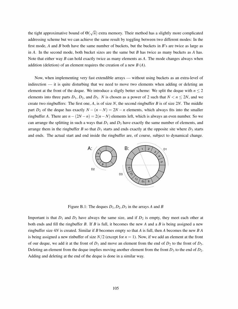
the tight approximative bound of Θ(√
n) extra memory. Their method has a slightly more complicated
addressing scheme but we can achieve the same result by toggling between two different modes: In thefirst mode, A and B both have the same number of buckets, but the buckets in B’s are twice as large as
in A. In the second mode, both bucket sizes are the same but B has twice as many buckets as A has.Note that either way B can hold exactly twice as many elements as A. The mode changes always when
addition (deletion) of an element requires the creation of a new B (A).
Now, when implementing very fast extendible arrays — without using buckets as an extra-level of
indirection — it is quite disturbing that we need to move two elements when adding or deleting anelement at the front of the deque. We introduce a sligtly better scheme: We split the deque with n ≤ 2
elements into three parts D1, D2, and D3. N is chosen as a power of 2 such that N < n ≤ 2N, and we
create two ringbuffers: The first one, A, is of size N, the second ringbuffer B is of size 2N. The middlepart D2 of the deque has exactly N− (n−N) = 2N − n elements, which always fits into the smaller
ringbuffer A. There are n− (2N−n) = 2(n−N) elements left, which is always an even number. So we
can arrange the splitting in such a ways that D1 and D3 have exactly the same number of elements, andarrange them in the ringbuffer B so that D1 starts and ends exactly at the opposite site where D3 starts
and ends. The actual start and end inside the ringbuffer are, of course, subject to dynamical change.
Figure B.1: The deques D1,D2,D3 in the arrays A and B
Important is that D1 and D3 have always the same size, and if D2 is empty, they meet each other at
both ends and fill the ringbuffer B. If B is full, it becomes the new A and a B is being assigned a newringbuffer size 4N is created. Similar if B becomes empty so that A is full, then A becomes the new B A
is being assigned a new rinbuffer of size N/2 (except for n = 1). Now, if we add an element at the front
of our deque, we add it at the front of D1 and move an element from the end of D2 to the front of D3.Deleting an element from the deque implies moving another element from the front D3 to the end of D2.
Adding and deleting at the end of the deque is done in a similar way.
105

106

Bibliography
[AHU 74] A.V. Aho, J.E. Hopcroft, J.D. Ullman The Design and Analysis of Algorithms. Addison-
Wesley, 1974
[AHT 00] S. Alstrup, J. Holm, M. Thorup Maintaining Center and Median in Dynamic Trees. Proc. 7thSWAT, LNCS 1851, 2000
[AHLT 03] S. Alstrup, J. Holm, K. de Lichtenberg, M. Thorup Maintaining Information in Fully-Dynamic Trees. The Computing Research Repository (CoRR) cs-DS-0310065, 2003
[Bar 04] N. Barraci Persistente Arrays zur Effizienten Speicherung sich Partiell Wiederholender Ob-jektketten. Diploma Thesis, Darmstadt University of Technology, 2004
[BCDMS 99] A. Brodnik, S. Carlsson, E.D. Demaine, J.I. Munro, R. Sedgewick Resizable Arrays inOptimal Time and Space. 6th International Workshop on Algorithms and Data Structures
(WADS) 1999
[BHKS] W. Brauer, M. Holzer, B. König, S. Schwoon The Theory of Finite State Adventures. EATCS
Bulletin, 79:230-237, 2003
[BJM 98] C. Barret, R. Jacob, M. Marathe Formal Language Constrained Path Problems. Los AlamosReserach Report LA-UR-98-1739, 1998
[Bur 02] J. Burghardt Maintaining Partial Sums In Logarithmic Time. Nordic Journal of Computation,2002
[CeDi 04] M. Cetti, S. Dingel Solution to an Exercise. private communication, 2004
[CoWi 90] D. Coppersmith, S. Winograd Matrix Multiplication Via Arithmetic Progression. Journal ofSymbolic Computation 9, 1990
[CLRS 01] T.H. Cormen, C.E. Leiserson, R.L. Rivest, C. Stein Introduction to Algorithms. The MIT
Press, 2001, second edition
[EGI 99] D. Eppstein, Z. Galil, G.F. Italiano Dynamic Graph Algorithms. in Algorithms and Theoryof Computation Handbook CRC Press, 1999
107
[Fre 85] G.N. Fredrickson Data Structures for OnlineUpdating of Minimum Spanning Trees. SIAM
Journal of Computing 14, 1985
[GaJo 79] M.R. Garey, D.S. Johnson Computers and Intractability — A Guide to the Theory of NP-Completeness. W.H. Freeman and Company, 1979
[Gli 03] O. Glier Kolmogorov Complexity and Deterministic Context-Free Languages. SIAM Journal
of Computing 32, 2003
[Gon 95] L. Gonick The Solution. Discover, April 1995
[Goo 98] J. T. Goodman Parsing Inside-Out. Thesis, Havard University, 1998
[Har 78] M.A. Harrison Introduction to Formal Language Theory. Addison-Wesley 1978
[Has 98] R. Hassin Approximation schemes for the restricted shortest path problem. Mathematics of
Operations Research, 17(1), 1992
[HeKi 99] M.R. Henzinger, V. King Randomized Fully Dynamic Graph Algorithms with Poly-Logarithmic Time per Operation. Journal of the ACM 46, 1999
[HLT 01] J. Holm, K. de Lichtenberg, M. Thorup Poly-Logarithmic Deterministic Fully-Dynamic Al-gorithms for Connectivity, Minimum Spanning Tree, 2-edge, and Biconnectivity. Journal of
the ACM 48, 2001
[Knu 73] D.E. Knuth The Art of Computer Programming Vol. 3, Sorting and Searching. Addison-
Wesley 1978
[KnPl 81] D.E. Knuth, M.F. PLass Breaking Paragraphs Into Lines. Software: Practice & Experience,
11(11), 1981
[Knu 77] D.E. Knuth A Generalization of Dijkstra’s Algorithm. Information Processing Letters 6, 1977
[Knu 98] D.E. Knuth The Art of Computer Programming Vol. 2, Seminumerical Algorithms. Addison-
Wesley 1998, third edition
[KuSa 85] W. Kuich, A. Salomaa Semirings, Automata, Languages. Springer-Verlag 1985
[Lee 02] L. Lee Fast Context-Free Parsing Requires Fast Boolean Matrix Multiplication. Journal of
the ACM 49(1), 2002
[Moh 02] M. Mohri Semiring Frameworks and Algorithms For Shortest-Distance Problems. Journal of
Automata, Languages and Combinatorics 7, 2002
[MoRa 95] R. Motwani, P. Raghavan Randomized Algorithms. Cambridge University Press, 1995
108

[Mor 01] B.B. Mortensen The Deque Class in the Copenhagen STL: First Attempt. CPH STL Report
2001-4, 2001
[Oka 98] C. Okasaki Purely Functional Data Structures. Cambridge University Press 1998
[Ren 02] K. Renz Algorithms and Data Structures for a Music Notation System based on GUIDOMusic Notation. Phd thesis, Technische Universität Darmstadt 2002
[Ryt 95] W. Rytter Context-Free Recognition via Shortest Paths Computation: A Version of Valiant’sAlgorithm. Theoretical Computer Science 143, 1995
[Sei 95] R. Seidel On the All-Pairs-Shortest-Paths Problem in Unweighted Undirected Graphs. Jour-
nal of Computing and System Sciences 51, 1995
[Val 74] L.G. Valiant General Context-Free Recognition in Less Than Cubic Time. Journal of Com-
puting and System Sciences 10, 1974
[Wal 84] H.K.-G. Walter A Simpe Proof of Valiant’s Lemma. Theoretical Informatics and Applica-
tions 20, 1986
[LiVi95] Ming Li and Paul Vitányi. A New Approach to Formal Language Theory by KolmogorovComplexity. SIAM J. Comput., 24:2, 1995
[LiVi97] Ming Li and Paul Vitányi An Introduction to Kolmogorov Complexity and Its Applications.
Second Edition Springer-Verlag, 1997

Oliver Glier – Curriculum vitae
16th January 1972, Frankfurt am Main, Germany
Ziegelhüttenweg 8660598 Frankfurt am Main
Germany
Career History
1999 - 2004 research assistant at the research group for Au-tomata Theory and Formal Languages (AFS), De-
partment of Computer Science, Darmstadt Univer-
sity of Technology, Germany2001 - 2002 one-year visit at Fakultas Ilmu Komputer, Universi-
tas Indonesia in Depok/Jakarta, Indonesia. DAADscholarship
1999 diploma in computer science with a minor in math-
ematics1992 - 1999 student of computer science and mathematics at
Darmstadt University of Technology, Germany.
1991 - 1992 community service at the Day Nursery Gartenstraße,Neu-Isenburg, Germany
1978 - 1991 elementary and grammar school, 1991 Abitur
Erklärung
Hiermit erkläre ich, die vorliegende Arbeit zur Erlangung des akademischen Grades
Dr.rer.nat. mit dem Titel “Persistent Arrays, Path Problems, and Context-free Languages”
selbständig und ausschließlich unter Verwendung der angegebenen Hilfsmittel erstellt zuhaben. Ich habe bisher noch keine Promotionsversuche unternommen.
Darmstadt, den Oliver Glier