permutations in concatenated zigzag codesetcamach/amssi/reports/zigzag.pdfhigher rates correspond to...

Permutations in Concatenated Zigzag Codes

California State Polytechnic University, Pomona

and

Loyola Marymount University

Department of Mathematics Technical Report

Shawn Abernethy Jr.∗, Cindy Lee†, Jasmin Uribe‡, Sai Michael Wentum Jr.§,

Laura Smith¶, Edward Mosteig‖

Applied Mathematical Sciences Summer InstituteDepartment of Mathematics & Statistics

California State Polytechnic University Pomona3801 W. Temple Ave.Pomona, CA 91768

August 4, 2007

∗Elizabethtown College†Loyola Marymount University‡University of Arizona§College of Charleston¶University of California, Los Angeles‖Loyola Marymount University, Los Angeles

1

Contents

1 Introduction 5

2 Objective 5

3 Zigzag Codes and Concatenated Zigzag Codes 63.1 Zigzag Codes . . . . . . . . . . . . . . . . . . . . . . . . . . . . . . . . . . . 63.2 Concatenated Zigzag Codes . . . . . . . . . . . . . . . . . . . . . . . . . . . 7

4 Permutations, Dispersion and Variance 94.1 Permutations and Dispersion . . . . . . . . . . . . . . . . . . . . . . . . . . . 9

4.1.1 Permutations Generated from Matlab’s randperm Command . . . . . 104.1.2 Permutation Generated from Matlab’s magic command . . . . . . . . 10

4.2 Theoretical Results Concerning Permutations . . . . . . . . . . . . . . . . . 114.3 Behavior of Average Dispersion . . . . . . . . . . . . . . . . . . . . . . . . . 114.4 Variance of a Permutation . . . . . . . . . . . . . . . . . . . . . . . . . . . . 134.5 Group Dispersion Table . . . . . . . . . . . . . . . . . . . . . . . . . . . . . 16

5 Triangular Difference Tables 19

6 Comparisons of Permutations in Concatenated Zigzag Codes 226.1 Background . . . . . . . . . . . . . . . . . . . . . . . . . . . . . . . . . . . . 226.2 Iterations of the Decode Process . . . . . . . . . . . . . . . . . . . . . . . . . 236.3 Reshaping the Information Matrix D . . . . . . . . . . . . . . . . . . . . . . 246.4 Classical Block Permutations . . . . . . . . . . . . . . . . . . . . . . . . . . 246.5 Algebraic Permutations . . . . . . . . . . . . . . . . . . . . . . . . . . . . . . 26

6.5.1 Fields and Monomial Orders . . . . . . . . . . . . . . . . . . . . . . . 266.5.2 The Construction of Algebraic Permutations . . . . . . . . . . . . . . 28

6.6 Structured Permutations by Tejas Bhatt and Victor Stolpman . . . . . . . . 29

7 Future Work 33

8 Acknowledgements 34

9 Programs 359.1 Zigzagsimualator . . . . . . . . . . . . . . . . . . . . . . . . . . . . . . . . . 35

9.1.1 RandMessage.m . . . . . . . . . . . . . . . . . . . . . . . . . . . . . . 379.1.2 Parities.m . . . . . . . . . . . . . . . . . . . . . . . . . . . . . . . . . 37

9.2 Permute.m . . . . . . . . . . . . . . . . . . . . . . . . . . . . . . . . . . . . . 389.2.1 codeword.m . . . . . . . . . . . . . . . . . . . . . . . . . . . . . . . . 399.2.2 tilde.m . . . . . . . . . . . . . . . . . . . . . . . . . . . . . . . . . . . 399.2.3 whitenoise.m . . . . . . . . . . . . . . . . . . . . . . . . . . . . . . . 409.2.4 Decode.m . . . . . . . . . . . . . . . . . . . . . . . . . . . . . . . . . 409.2.5 calcLe.m . . . . . . . . . . . . . . . . . . . . . . . . . . . . . . . . . . 419.2.6 calcF.m . . . . . . . . . . . . . . . . . . . . . . . . . . . . . . . . . . 42

2

9.2.7 calcB.m . . . . . . . . . . . . . . . . . . . . . . . . . . . . . . . . . . 429.2.8 calcW.m . . . . . . . . . . . . . . . . . . . . . . . . . . . . . . . . . . 439.2.9 calcLo.m . . . . . . . . . . . . . . . . . . . . . . . . . . . . . . . . . . 439.2.10 clip.m . . . . . . . . . . . . . . . . . . . . . . . . . . . . . . . . . . . 449.2.11 FinalLLR.m . . . . . . . . . . . . . . . . . . . . . . . . . . . . . . . . 44

9.3 Permutations . . . . . . . . . . . . . . . . . . . . . . . . . . . . . . . . . . . 459.3.1 Right to Left/Top to Bottom . . . . . . . . . . . . . . . . . . . . . . 459.3.2 Right to Left/Bottom to Top . . . . . . . . . . . . . . . . . . . . . . 459.3.3 Left to Right/Top to Bottom . . . . . . . . . . . . . . . . . . . . . . 469.3.4 Left to Right/Bottom to Top . . . . . . . . . . . . . . . . . . . . . . 469.3.5 Permutation Presented by Tejas Bhatt and Victor Stolpman . . . . . 479.3.6 conditionA.m . . . . . . . . . . . . . . . . . . . . . . . . . . . . . . . 499.3.7 conditionB.m . . . . . . . . . . . . . . . . . . . . . . . . . . . . . . . 499.3.8 un3d.m . . . . . . . . . . . . . . . . . . . . . . . . . . . . . . . . . . 509.3.9 Randomly Permuting Each Column . . . . . . . . . . . . . . . . . . . 509.3.10 Randomly Permute Each Column with a Restriction . . . . . . . . . 519.3.11 swapperperm.m . . . . . . . . . . . . . . . . . . . . . . . . . . . . . . 539.3.12 Magic Square Permutation . . . . . . . . . . . . . . . . . . . . . . . . 539.3.13 throwupperm.m . . . . . . . . . . . . . . . . . . . . . . . . . . . . . . 549.3.14 flatten.m . . . . . . . . . . . . . . . . . . . . . . . . . . . . . . . . . . 559.3.15 swapprows.m . . . . . . . . . . . . . . . . . . . . . . . . . . . . . . . 559.3.16 horazontalswrill.m . . . . . . . . . . . . . . . . . . . . . . . . . . . . 56

9.4 Dispersion and their Measurements . . . . . . . . . . . . . . . . . . . . . . . 569.4.1 sumvarows.m . . . . . . . . . . . . . . . . . . . . . . . . . . . . . . . 569.4.2 dispoflistofpermswithinvers.m . . . . . . . . . . . . . . . . . . . . . 579.4.3 inverseperm.m . . . . . . . . . . . . . . . . . . . . . . . . . . . . . . . 589.4.4 compute2perms.m . . . . . . . . . . . . . . . . . . . . . . . . . . . . . 58

9.5 Triangular Distance and Random Walks . . . . . . . . . . . . . . . . . . . . 59

3

Abstract

Coding theory is a branch of mathematics, computer science and electrical engi-neering that explores the transmission of information across noisy channels. Codingtheory is used in data transmission, data storage, and telecommunications. The focusof this project is on concatenated zigzag codes, which are constructed using permuta-tions. We study the effects of permutations on the error-correcting capabilities of thecoding scheme. In conjunction, we explore the behavior of average dispersion in orderto further our understanding of randomness of a permutation and find correspondencewith error-correction.

4

1 Introduction

Coding theory is the study of the transmission of data across a noisy channel with theultimate goal of successfully recovering the data to its original form from an error-riddenmessage. Since a message may be corrupted upon transmission across the noisy channel,error-correcting measures must be taken in order to ensure that the receiver can reconstructthe original codeword. This study works to improve the error-correcting capabilities ofcertain codes while maintaining reasonable transmission time.

It is important to note that coding theory is neither cryptography nor steganography.Although the term coding theory is often confused with both of these forms of communica-tion, coding theory is an entirely different field of study. Steganography is literally translatedas covered writing and is not largely used in practice. It simply refers to sending messageshidden from the naked eye. One example is tattooing a message on someone’s head and thenletting their hair grow, thus covering up the message. The receiver, however, knows wherethe message is located and simply removes the hair and reads the message. Steganography isnot secure because an interceptor only needs to find the location of the message. Cryptogra-phy, on the other hand, is much more secure. It literally means hidden writing, which meansthat even if the message is intercepted only the sender and receiver have the predeterminedalgorithm that encrypts and decrypts the message. In coding theory, however, one does notattempt to hide the message; rather, one adds redundancy to a message to overcome errorsthat are introduced during transmission.

The performance of an encoding scheme is measured by its error-correcting capabilitiesand its rate, which is defined as the ratio of the number of information bits to the numberof total bits sent.

rate =# information bits

# total bits. (1)

Higher rates correspond to faster transmission since more information bits are transmittedper total bits. However, transmissions with high rates are more prone to uncorrectable errorsbecause there is less redundancy present in the transmission. Thus, it is desirable to find anideal rate that minimizes transmission time but maximizes error correction.

Coding theory is used in many places. An example of this is NASA, which uses codingtheory for sending and receiving transmissions across space. It can also be found in everydaylife ranging from data storage in CDs and DVDs to wireless communications. Currently,engineers from Nokia are applying for patents regarding specific components of a class ofcodes called concatenated zigzag codes. The focus of our research is on optimizing theerror-correcting capabilities of concatenated zigzag codes.

2 Objective

This project explores the relationship between permutations and their role in the error-correcting capabilities of concatenated zigzag codes. Through examining permutations andanalyzing their effects on error-correction, we hope to find a specific type of permutation thatreduces error rates. One of the properties we focus on is the behavior of the dispersion ofpermutations. Dispersion is a measure of the randomness of a permutation. In conjunction,

5

we explore the behavior of average dispersion in order to further our understanding of therandomness in a permutation and find a correspondence with error-correction, if any. Finally,we create a new way of analyzing permutations using variance and group dispersion tables.

3 Zigzag Codes and Concatenated Zigzag Codes

The coding process is made up of three basic parts: encoding, transmission through noisychannels, and decoding.

A message is encoded using a predetermined coding scheme, which can be as simple oras complex as the sender desires. A codeword is defined as any output of an encodingscheme. The codeword is what is transmitted. During transmission, noise may introduceerrors to the codeword, resulting in corruption of the message. This error-ridden message isthen received by the intended recipient and decoded using specific decoding algorithms.

3.1 Zigzag Codes

Zigzag codes can be described using the following graph, where the white nodes are informa-tion bits and the black nodes are parity bits. We use I to denote the number of segments inthe graph and J to denote the number of information bits on each segment. In other words,I denotes the total number of parity bits and J denotes the number of information bits perparity bit. In this particular example, I = 3 and J = 2.

The information bits are denoted using the notationd(i, j), where i is the number of the segment on which thenode lies and j refers to the specific position within thatsegment. The parity bits are denoted by p(i), where thecorresponding node lies at the end of segment i.

In the case of zigzag codes the encoding process con-sists of computing the redundant parity bits. These par-ity bits are calculated by adding all previous nodes on thesame segment using the following equations:

p(1) =J∑

j=1

d(i, j) mod 2;

p(i) =J∑

j=1

d(i, j) + p(i− 1) mod 2, for i = 2, 3..., I.

For example, consider the message [011001]. Withthe aid of the diagram, we compute the parity bits.

6

To calculate the first parity bit, the bits of the firstsegment are added together modulo two:

p(1) = d(1, 1) + d(1, 2) = 0 + 1 = 1.

The second parity bit is the sum of the first parity bitand the information bits lying on the segment:

p(2) = p(1)+d(2, 1)+d(2, 2) = 1+1+0 = 2 mod 2 = 0.

The subsequent parity bits are calculated in a similarmanner.

Redundancy introduced by the parity bits ensuresthat more errors will be corrected during the decodingprocess, thus increasing the error-correcting capabili-ties of the code.

To facilitate the encoding and decoding process,the information bits and parity bits are stored in the matrix D and the vector P, respectively.

D =

0 11 00 1

P =

101

Referring to the zigzag code diagram, we create matrices for calculations. The I × J

matrix, D, is derived by taking each of the information bits from a given segment of thediagram and placing them in the corresponding row of D. The column vector P is obtainedby reading the parity bits from the zigzag diagram top to bottom.

3.2 Concatenated Zigzag Codes

Zigzag codes by themselves have poor error-correcting capabilities. However, they haveexcellent transmission rates, namely J

J+1. Concatenated zigzag codes are used to increase

error-correction. Although These codes have excellent error-correcting capabilities, they havea lower rate.

Concatenated zigzag codewords are created by first creating K copies of the message D.Each replica is fed through one of the permutations, π1, π2, ...πK (for background info onpermutations, see Section 4.1). For each πk(D), the parity vector Pk is computed by usinga constituent zigzag code. Finally, the codeword is formed by concatenating the matrix Dwith the parity vectors P1, P2, ..., PK .

7

The figure above is a graphical representation of the encoding process using a concate-nated zigzag encoder. The message, D, is replicated, permuted, and encoded. Then theparity vectors, P1, P2, ..., PK , are concatenated with D and sent through the noisy channelas the codeword.

To decode, we implemented the Max-Log-APP (MLA) process of decoding zigzag codesoriginally presented by Li Ping in [Pi(2)] and later presented by Tejas Bhatt and VictorStolpman in [Bh]. Using MLA, the decoding process computes forward and backward ex-trinsic information for the parity bits of the kth permutation for each of the sub-iterations.This constructs a single iteration of the decoding process.

To form the codeword, the I × J message matrix D and the parity vectors P1, P2, ..., PK

are concatenated. The 0s of the codeword are then changed to 1s and the 1s are then changedto -1s. It is this modulated codeword that is transmitted to the receiver.

The receiver then reconstructs the message matrix, and the parity vectors received withpossible corruption. The received message matrix is denoted D̃ and the parity vectors asP̃1, P̃2, ..., P̃K . Let P̃k be the received parity vector corresponding to the kth permutation.The receiver then uses the parity vectors to correct any errors introduced to the receivedmessage with the following equations:

• Max-log approximation:

W (z1, z2, ..., zn) =[Πn

j=1sign(zj)]·min1≤j≤n|zj|

• Forward recursion:

F [q](pk(i)) = p̃k(i) + W(F [q](pk(i− 1)), L[q]

o (dk(i, 1)), ..., L[q]o (dk(i, J))

)where i = 1, 2, . . . , I and F [q](pk(0)) = +∞

• Backward recursion:

B[q](pk(i− 1)) = p̃k(i− 1) + W(L[q]

o (dk(i, 1)), ..., L[q]o (dk(i, J)), B[q](pk(i))

)where i = I − 1, ..., 2, 1 and B[q](p̃k(I)) = p̃(I)

• Extrinsic Information

L[q]e (dk(i, j)) = W

(F [q](pk(i− 1)), L

[q]o (dk(i, 1)), ..., L

[q]o (dk(i, j − 1)),

L[q]o (dk(i, j − 1)), ..., L

[q]o (dk(i, J)), B[q](pk(i))

)

L[q]o (dk(i, j)) = πk

[d̃(i, j) +

∑k′<k

[π−1k′ [L[q]

e (dk′(i, j))]] +∑k′>k

[π−1k′ [L[q−1]

e (dk′(i, j))]]

],

where Lo is initialized as an I × J matrix of zeros.

• Final Log Likelihood Ratio Computation

L[q](d(i, j)) = d̃(i, j) +K∑

k=1

π−1k

[L[q]

e (dk(i, j))]

The receiver then takes the sign of all the entries in the I ×J matrix L[q]. The larger themagnitudes of the entries in L[q], the more probable that entry is a 1 or -1. The receiver thendemodulates the matrix to construct the message – hopefully the original message sent.

8

4 Permutations, Dispersion and Variance

As we previously stated, the focus of our project is to determine which sets of permutationsoptimize error-correction in concatenated zigzag codes. One of the focuses of this section ison dispersion, a measure of the randomness of a permutation. Since we are working witha set of permutations, using the dispersion of a single permutation will not suffice as apredictor of performance of concatenated zigzag codes. This requires the creation of whatwe call group dispersion tables. In addition, we study the variance of a permutation, whichis a possible way of measuring how a certain row is permuted with respect to other rows ofthe message matrix.

4.1 Permutations and Dispersion

Definition 1. A permutation of set size n is defined to be any bijection π : [n] → [n]where [n] denotes {1, 2, 3, ..., n}.

Consider the following permutation of [5]:

π =

(1 2 3 4 54 3 1 5 2

).

This notation represents π(1) = 4, π(2) = 3, π(3) = 1, π(4) = 5 and π(5) = 2.To measure the randomness of a permutation we use a metric known as dispersion. To

properly define the dispersion of a permutation, we need to make a preliminary construction.

Definition 2. Given a permutation π : [n] → [n], the list of differences of π is given by

DL(π) = {(j − i, π(j)− π(i)) | 1 ≤ i < j ≤ n}. (2)

Let |DL(π)| denote the number of unique elements of DL.

Definition 3. The dispersion of π is a normalized measure of the number of unique orderedpairs that appears in the list of differences, computed as:

disp(π) =|DL(π)|(

n2

) . (3)

Note that 0 < disp(π) ≤ 1 for any permutation, where a dispersion of 0 indicates ahighly structured permutation and 1 is a random permutation. To illustrate this definition,we compute the dispersion of the following permutation:

π =

(1 2 3 43 4 1 2

).

The elements of DL(π) are given in the following table:Finally, we find the dispersion by counting the number of distinct ordered pairs in DL(π)

and dividing by(

n2

). In this particular case, there are two repeated ordered pairs, (1,1) and

(2,-2), and so there are only four unique ordered pairs. Therefore,

disp(π) =|DL(π)|(

n2

) =4(42

) =4

6=

2

3.

9

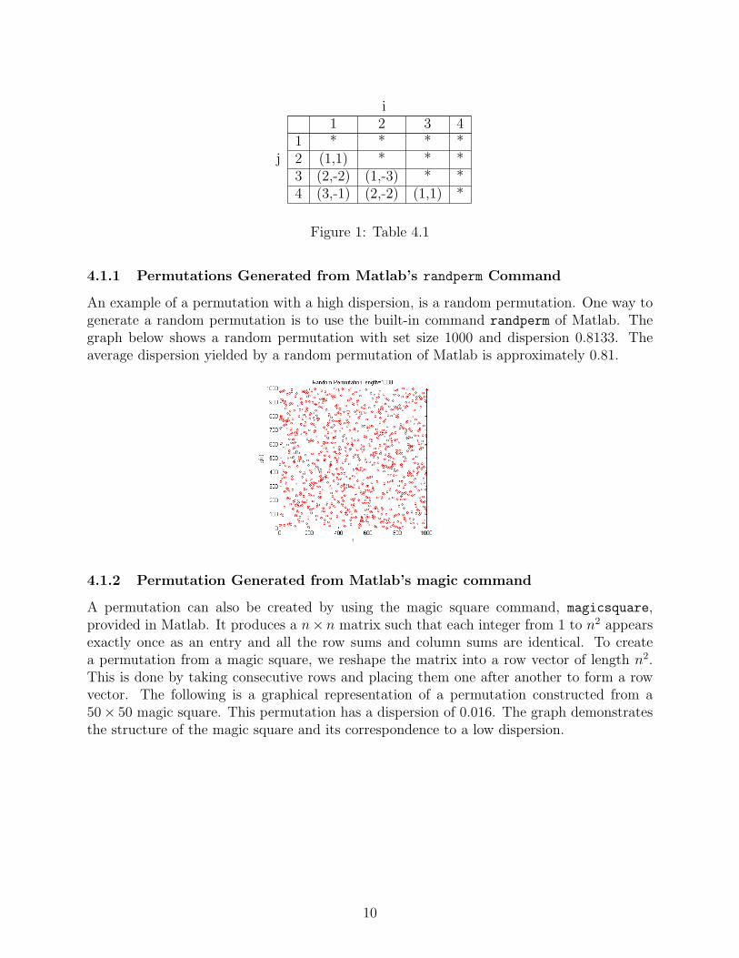
i1 2 3 4

1 * * * *j 2 (1,1) * * *

3 (2,-2) (1,-3) * *4 (3,-1) (2,-2) (1,1) *

Figure 1: Table 4.1

4.1.1 Permutations Generated from Matlab’s randperm Command

An example of a permutation with a high dispersion, is a random permutation. One way togenerate a random permutation is to use the built-in command randperm of Matlab. Thegraph below shows a random permutation with set size 1000 and dispersion 0.8133. Theaverage dispersion yielded by a random permutation of Matlab is approximately 0.81.

4.1.2 Permutation Generated from Matlab’s magic command

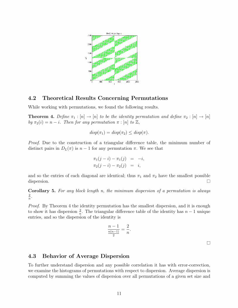
A permutation can also be created by using the magic square command, magicsquare,provided in Matlab. It produces a n× n matrix such that each integer from 1 to n2 appearsexactly once as an entry and all the row sums and column sums are identical. To createa permutation from a magic square, we reshape the matrix into a row vector of length n2.This is done by taking consecutive rows and placing them one after another to form a rowvector. The following is a graphical representation of a permutation constructed from a50× 50 magic square. This permutation has a dispersion of 0.016. The graph demonstratesthe structure of the magic square and its correspondence to a low dispersion.

10

4.2 Theoretical Results Concerning Permutations

While working with permutations, we found the following results.

Theorem 4. Define π1 : [n] → [n] to be the identity permutation and define π2 : [n] → [n]by π2(i) = n− i. Then for any permutation π : [n] to Z,

disp(π1) = disp(π2) ≤ disp(π).

Proof. Due to the construction of a triangular difference table, the minimum number ofdistinct pairs in DL(π) is n− 1 for any permutation π. We see that

π1(j − i)− π1(j) = −i,

π2(j − i)− π2(j) = i,

and so the entries of each diagonal are identical; thus π1 and π2 have the smallest possibledispersion.

Corollary 5. For any block length n, the minimum dispersion of a permutation is always2n.

Proof. By Theorem 4 the identity permutation has the smallest dispersion, and it is enoughto show it has dispersion 2

n. The triangular difference table of the identity has n− 1 unique

entries, and so the dispersion of the identity is

n− 1n(n−1)

2

=2

n.

4.3 Behavior of Average Dispersion

To further understand dispersion and any possible correlation it has with error-correction,we examine the histograms of permutations with respect to dispersion. Average dispersion iscomputed by summing the values of dispersion over all permutations of a given set size and

11

then dividing by the total number of permutations of that set size. The following equationis used to calculate the average dispersion of all permutations of set size n:

average disp(n) =1

n!

∑π∈Sn

disp(π).

For set size 2 the average dispersion of a given permutation is 1; since there are 2 possiblepermutations both with dispersion 1, thus the average dispersion is 1+1

2= 1. For set sizes

up to 10, it is possible to compute the dispersion of all permutations. However, for largerset sizes, only a sample of the total number of permutations is used to calculate the averagedue to constraints on computing power and time.

The following histograms show the distribution of permutations with respect to disper-sion.

From these distributions, it can be seen that as the set size increases, the proportion ofpermutations with dispersion between 0.8 and 0.9 increases. Since producing a histogram forthe dispersion of all permutations of set size n > 10 is computationally infeasible, samplingis necessary due to the memory constraints of our computers.

The graph below demonstrates the asymptotic behavior of the average dispersion withrespect to set size. In fact, the average dispersion approaches a constant around 0.81.

12

The behavior demonstrated by the distribution of average dispersion can be approximatedby a sum of two exponential functions: disp(n) = 4.5964−1.7533n + 0.06661.7533n + 0.8173. Itis unknown whether average dispersion has an asymptote at a value around 0.81, or whetherit approaches 0. The following table shows the set size, the average dispersion, the standarddeviation and the sample size of each set size examined (if n >10). The table suggests thestandard deviation is approaching 0 and the dispersion is approaching a value around 0.81.

n Average Dispersion Standard Deviation Sample Size2 1 0 23 0.8888888 0.1721326 64 0.8472222 0.1766343 245 0.8466666 0.1494715 1206 0.8383333 0.1273568 7207 0.8355253 0.0656522 50408 0.8318895 0.0866602 403209 0.8300064 0.0737352 36288010 0.8280427 0.0656522 362880011 0.8268012 0.0581352 3000000012 0.8254789 0.0534279 3000000013 0.8246220 0.0488241 3000000014 0.8237070 0.0451643 3000000015 0.8230517 0.0419172 3000000016 0.8223984 0.0391362 3000000017 0.8218721 0.0366868 3000000018 0.8213694 0.0345478 3000000019 0.8209739 0.0326291 3000000020 0.8205578 0.0309247 3000000030 0.8182114 0.0203068 3000000040 0.8170504 0.0151259 1000000050 0.8163426 0.0120574 1000000060 0.8158753 0.0100037 1000000070 0.8155449 0.0085911 1000000080 0.8152998 0.0075097 1000000090 0.8151062 0.0066752 10000000100 0.8149514 0.0060031 10000000200 0.8142764 0.0030067 10000000300 0.8140503 0.0020198 10000000400 0.8139387 0.0015189 10000000500 0.8138702 0.0012231 10000000600 0.8138251 0.0010271 10000000700 0.8137924 0.0008843 10000000

4.4 Variance of a Permutation

In general, there are a lot of ways to construct permutations. For various classes of permu-tations, their performance in concatenated zigzag codes is well-known. For example, as weshall see in this section, any of the classical block permutations have very poor performance.In contrast, randomly-generated permutations have excellent performance. Since there areso many different permutations it would be useful if there were a way to quantify how wella permutation would perform before running time-intensive simulations.

Definition 6. Define the symmetric group, Sn, to be the collection of all the permutationsof [n] = {1, 2, . . . , n}.

13

Definition 7. Given integers I, J and a set S, denote the set of all I × J matrices whoseentries take on values from the set S by

MatI,J(S).

Definition 8. Given positive integers I, J , define

ρI,J : SIJ → MatI,J({1, . . . , IJ})

to be the function that takes a permutation π ∈ SIJ and produces the I × J matrix whose(i, j) entry is π((i−1)J + j). That is, ρI,J places the values π(1), π(2), . . . , π(IJ) in an I×Jmatrix row-by-row.

Definition 9. Given positive integers I, J , define

βI,J : SIJ → MatI,J({1, . . . , IJ})

to be the function that takes in a permutation π and produces the I × J matrix, the rowcorrelation matrix RCMI,J(π) whose (i, j)th entry is⌈

ρI,J(π)

I

⌉.

Definition 10. Let π ∈ Sn be a permutation, and let I, J be positive integers such thatn = IJ . Then the (I, J)-variance of a permutation is the sum of the population varianceof the rows of RCMI,J(π); that is,

varI,J(π) =I∑

i=1

J∑j=1

1

J(mij −

1

j

J∑j=1

mi,j)2,

where M = (mi,j) = βI,J(π).

Example 11. Consider the permutation

π =

(1 2 3 4 5 6 7 8 9 1010 2 9 4 7 6 3 8 1 5

).

Evaluating the mapping β2,5 at the permutation π, we get

β2,5(π) =

(2 1 2 1 22 1 2 1 1

).

The mean of the first row is2 + 1 + 2 + 1 + 2

5= 1.6,

and the mean of the second row is

2 + 1 + 2 + 1 + 1

5= 1.4.

14

The population variance of the first and second rows of β2,5(π) are

(2− 1.6)2 + (1− 1.6)2 + (2− 1.6)2 + (1− 1.6)2 + (2− 1.6)2

5= .24

and(2− 1.4)2 + (1− 1.4)2 + (2− 1.4)2 + (1− 1.4)2 + (1− 1.4)2

5= .24,

respectively. Thus, the (2, 5)-variance of π is 0.48.

A problem with the variance of a permutation is that unlike dispersion, variance doesnot have a natural normalized value between 0 and 1. Since variance tends to increase withset size, it is hard to compare permutations of significantly different set sizes. Thus, for agiven set size, we wish to create an upper-bound for the variance. We would then be ableto divide the variance by the upper bound, thus producing a normalized value that rangesbetween 0 and 1. We make a conjecture concerning this upper bound in the case I = J.

Proposition 12. Let π : [n2] → [n2] be a permutation such that every row of βn,n(π) consistsof the entries 1 through n in some order. Then the (n,n)-variance of βn,n(π) is

n3 − n

12.

Proof. Let x be a row that appears in βn,n(π). Then x is a vector with n entries and it hasone occurrence of each of the numbers 1, 2, . . . , n. By Definition 10, the variance of one rowis

1

n

n∑i=1

(xi − x̄)2

where x̄ = 1n

∑xi. Thus, the total variance for the n rows is

n · 1

n

n∑i=1

(xi − x̄)2 =n∑

i=1

(i− x̄)2 (4)

It is well known thatn∑

i=1

i =n(n + 1)

2,

and so

15

n∑i=1

(i− x̄)2 =n∑

i=1

(i− (n + 1)

2

)2

=n∑

i=1

(i2 − i(n + 1) +

(n + 1)2

4

)=

n∑i=1

i2 −n∑

i=1

i(n + 1) +n∑

i=1

(n + 1)2

4

=n∑

i=1

i2 − (n + 1)n∑

i=1

i +(n + 1)2

4

n∑i=1

1

=n(n + 1)(2n + 1)

6− n(n + 1)(n + 1)

2+

n(n + 1)2

4

= n(n + 1)

(2(2n + 1)− 6(n + 1) + 3 (n + 1)

12

)= n(n + 1)

((4n + 2)− (6n + 6) + (3n + 3)

12

)=

n(n + 1)(n− 1)

12

=n3 − n

12.

Conjecture 13. For any π ∈ Sn2 the maximum (n, n)-variance possible for π is n3−n12

.

4.5 Group Dispersion Table

Since concatenated zigzag codes utilize a set of permutations, the dispersion of a singlepermutation is not the defining measure of the performance of the set. A possible predictivemeasure of the performance of a set of permutations, however, may be found in the groupdispersion table.

Definition 14. Given a set of K permutations, the group dispersion table is a lower-triangular matrix M such that

M(i, j) =

{D(πiπ

−1j ) for i < j;

0 otherwise.

Definition 15. Given permutations π1, . . . , πk ∈ Sn, the average dispersion distance of{π1, . . . , πk} is the average of the nonzero entries of the group dispersion table.

The following graphs demonstrate that two permutations π1, π2 with high dispersion canyield a permutation π1π

−12 with low dispersion.

16

Example of a randomly generated permutation, π1 with dispersion of 0.8155.

Example of an algebraic permutation, π2 with dispersion 0.8178.

Example of the composition of the two permutations, π1π−12 with a dispersion of 0.3410.

Thus the average dispersion distance is defined so that we have a measure of how differentthe permutations in a collection are from one another.

Example 16. Consider the set of 7 permutations in S10 defined as

17

π1 =

(1 2 3 4 5 6 7 8 9 101 2 3 4 5 6 7 8 9 10

),

π2 =

(1 2 3 4 5 6 7 8 9 101 3 5 7 9 2 4 6 8 10

),

π3 =

(1 2 3 4 5 6 7 8 9 102 4 6 8 10 1 3 5 7 9

),

π4 =

(1 2 3 4 5 6 7 8 9 1010 9 8 7 6 5 4 3 2 1

),

π5 =

(1 2 3 4 5 6 7 8 9 101 4 6 7 9 10 2 3 5 8

),

π6 =

(1 2 3 4 5 6 7 8 9 106 7 8 9 10 1 2 3 4 5

),

π7 =

(1 2 3 4 5 6 7 8 9 109 8 7 6 5 4 3 2 1 10

).

As an intermediate step toward constructing the group dispersion table, we place thefollowing permutations in a table before computing the values of dispersion:

i1 2 3 4 5 6 7

1 0 0 0 0 0 0 02 π1π

−12 0 0 0 0 0 0

3 π1π−13 π2π

−13 0 0 0 0 0

j 4 π1π−14 π2π

−14 π3π

−14 0 0 0 0

5 π1π−15 π2π

−15 π3π

−15 π4π

−15 0 0 0

6 π1π−16 π2π

−16 π3π

−16 π4π

−16 π5π

−16 0 0

7 π1π−17 π2π

−17 π3π

−17 π4π

−17 π5π

−17 π6π

−17 0

Taking the dispersion of every nonzero entry, we obtain the following table:

i1 2 3 4 5 6 7

1 0 0 0 0 0 0 02 0.2889 0 0 0 0 0 03 0.2889 0.4000 0 0 0 0 0

j 4 0.2000 0.2889 0.2889 0 0 0 05 0.5778 0.5778 0.5111 0.5778 0 0 06 0.2889 0.4000 0.4000 0.2889 0.6000 0 07 0.3778 0.4667 0.4667 0.3778 0.4889 0.3111 0

Summing the entries in the group dispersion table, we obtain a value of 8.4667, andso the average of the nonzero entries is 8.4667

21= 0.4032. Thus, for this particular set of

permutations, the average dispersion distance is 0.4032.

18

5 Triangular Difference Tables

To simplify calculations and to examine patterns among the ordered pairs of table 4.1, thetable can be condensed to include only the second component of each ordered pair. Tofind the number of unique elements of DL(π), consider any repetitions in each diagonal.This condensed DL(π) table is known as the triangular difference table (TDT). To computedispersion using the TDT, sum the counts of the number of unique entries in each diagonaland then divide by the total number of integer entries in the table. This is described moreformally in Definition 17 below and in Lemma 41.

Definition 17. Let π : [n] → [n] be a permutation. We define the triangular difference tableof π to be the lower-triangular (i.e., below the main diagonal) portion of the n × n matrixwhose (i, j) entry (where i < j) is given by

π(j + 1)− π(i). (5)

Thus, the (i, j) entry of the TDT is π(j + 1)− π(i). Note that the triangular differencetable has n− 1 rows and n− 1 columns with different numbers of numerical entries.

Because the triangular distance table can be found using the list of differences, where thefirst components in each diagonal are the same, the values are only compared within its owndiagonal. In other words, when looking for distinct values, or the number of distinct valuesin a TDT, only the comparisons within diagonals are taken into consideration.

Example 18. Given the permutation(1 2 3 44 3 1 2

),

the corresponding triangular TDT is

−1−3 −2−2 −1 1

.

In this case, although -1 appears in both the 1st and 3rd rows, because they are in differentdiagonals, they are considered unique. (Same for the -2s).

Lemma 19. Given a permutation π of [n] and an integer 1 ≤ a ≤ n − 1, the number ofentries in the triangular difference table of π whose absolute value is a must be n− a.

Proof. Let π be a permutation in Sn and let a ∈ [n− 1]. There are n− a pairs i, j such that|j− 1| = a, namely, (1, a+1), (2, a+2), ..., (n−a, n). Thus, there are n−a pairs of the form(π(i), π(j)) such that |π(j)− π(i)| = a.

Lemma 20. Let π : [n] → [n] be a permutation and let A = (ai,j) be the correspondingtriangular difference table. Then ai,j is the sum of the ith through jth entries of the diagonal;that is,

ai,j =

j∑`=i

a`,`. (6)

19

Proof. By Definition 17, we know that

ai,j = π(j + 1)− π(i).

Thus,ai,j = [π(j + 1)− π(j)] + [π(j)− π(j − 1)] + ... + [π(i + 1)− π(i)]

= ajj + a(j − 1)(j − 1) + ... + aii.

Using this result, the relationship between the main diagonal and the rest of the numericalentries in the table can be seen.

Lemma 21. Given a permutation π1 : [n] → [n], define π2 : [n] → [n] by

π2(i) = n− π1(i).

Then the triangular difference tables of π1 and π2 are the negative transposes of one another.

Proof. Let A = (aij) and B = (bij) be the TDTs of π1andπ2, respectively. Then

bij = π2(j + 1)− π2(i) (7)

= (n− π1(j + 1))− (n− π1(i)) (8)

= −(π1(j + 1)− π1(i)) (9)

= −aij. (10)

By the definition of a triangular difference table, it is known that for each TDT thereexists a permutation that generates it. An interesting question is whether or not a TDT canbe generated by more than one permutation.

Theorem 22. Each triangular difference table is generated by a unique permutation.

Proof. Let ∆(π) be the main diagonal of a TDT, M. By Lemma 19, for some k, l, the (k, l)entry of the TDT, M , is n− 1. So for any permutation π with the given TDT, M ,

π(l + 1)− π(k) = n− 1,

and so,π(l + 1) = n.

In other words, π(l+1) is determined by M . Since (π(2)−π(1), π(3)−π(2), ..., π(n)−π(n−1))is determined by M , one can use this information in conjunction with the fact π(l + 1) = nto solve for π(1), π(2), ..., π(n).

Definition 23. Given a permutation π of set size n with TDT A = (aij), the main diagonalof π is the diagonal from a1,1 to an−1,n−1 of A. In particular, it is defined as

∆π = [π(2)− π(1), π(3)− π(2), ..., π(n)− π(n− 1)]. (11)

20

Definition 24. Given a vector v = (v1, ..., vn) ∈ Rn, define the absolute value of v by

|v| = (|v1|, ..., |vn|) ∈ Rn.

If d is the diagonal of a TDT, then (−d) is the diagonal of another TDT. The relation-ship of permutations that generate such TDTs is given in Lemma 21. Studying the absolutevalues of the entries in the diagonals and the signs of the entries in the diagonals, we posethe following two conjectures.

Conjecture 25. Let π ∈ Sn, where n is odd. Let (d1, ..., dn) = ∆π. If |di| = |dn−i| for all1 ≤ i ≤ n− 1, then di = dn−i for all 1 ≤ i ≤ n− 1.

Conjecture 26. The number of the permutations whose TDTs have palindromic diagonalsis divisible by 4.

Now, we count the number of potential candidates for the diagonal of a TDT. We call avector v ∈ [n− 1] a candidate if for any 1 ≤ i ≤ n− 1, at most n− i of the components ofv have absolute value i (i.e, the vector v satisfies the condition of Lemma 19).

Note that not all candidates are actually diagonals of TDTs.To find these candidates, we use exponential generating functions, which are defined as

follows.

Definition 27. The exponential generating function of the sequence (ao, a1, a2, ...) isdefined by

g(x) =∞∑

n=0

anxn

n!. (12)

Definition 28. The number of candidates of set size n is denoted

dn = {v ∈ Rn−1| v is a candidate}.

We calculate dn using exponential generating functions. The exponential generatingfunction can calculate the number of the absolute values of the entries of ∆π. Since thereare up to n− j possible occurrences of j in the TDT, we use the following as a factor of ourexponential generating function given by (12):

gj(x) =

n−j∑i=0

xi

i!.

By the theory of exponential generating functions (see [Tu]), dn is the coefficient of xn−1 in

n−1∏j=1

gj(x).

21

Example 29. Let n = 4. In any candidate vector, there may be up to 3, 2, and 1 occur-rences of 1,2, and 3, respectively. In the exponential generating function, the number 1 isrepresented by (1 + x + x2

2!+ x3

3!), 2 is represented by (1 + x + x2

2!), and 3 is represented by

(1 + x).Thus, we have the following exponential generating function:

g(x) = (1 + x +x2

2!+

x3

3!)(1 + x +

x2

2!)(1 + x) =

∞∑q=0

aqxq

q!.

The coefficient of x3

3!is a3 = 19, which means that there are 19 candidates of vector length

3 for n = 4.

6 Comparisons of Permutations in Concatenated Zigzag

Codes

In this section we outline the results obtained by running simulations that compare theperformance of various permutations when implemented in concatenated zigzag codes.

6.1 Background

Permutations are a main component in the construction of concatenated zigzag codes. Oneof the primary goals of this project is to determine what kinds of permutations and which setsof permutations improve error-correcting capabilities. In order to do this, Zigzagsimulator,a Matlab program, was created. The simulator takes in the dimensions of the message, thepermutation(s), the signal to noise ratios (SNR) to be tested and the number of iterationsthe decoding process is to perform. The program returns a graph of the signal to noise ratioversus the bit-error-rate (BER) which is defined as the number of uncorrectable bits to thetotal bits transmitted.

Zigzagsimulator includes a random message generator, an encoder that is fed permuta-tions, a noise generator, a decoder and a way of checking the uncorrectable errors remainingafter the decoding process.

To create a message, a simple algorithm was written to generate a random message ofspecified dimensions by the user. The encoding process was simulated by a program thatreplicated the message matrix a specified number of times, K, then permuted Kreplicaswith permutations given by the user. Each is run through the zigzag encoding process andthe parity matrices are computed. Finally, these K parity matrices are concatenated withthe original message and transmitted as a codeword through the noise generating algorithm.This specific noise generation algorithm simulates additive white Gaussian noise.

Finally, the codeword is received and decoded. The decoding algorithm uses the decodingequations presented by Tejas Bhatt and Victor Stolpman in [Bh] from work previously doneby Li Ping in [Pi(2)]. These algorithms use the redundancy provided by parity bits to finderrors in the received word. Belief propagation is used to determine the most probablemessage. Belief propagation is an algorithm that calculates the probability that a certain bitis either a 0 or a 1. The number of iterations tells the decoding algorithm how many times

22

to cycle through the decoding process, calculate probabilities and allow each permutation tocheck itself against the others. This process ensures that only the most probable message isreturned after decoding.

The last step of the simulation compares the decoded message to the original message,counting the number of differences, or uncorrectable errors. The lower the BER, the bettererror-correcting capabilities of the code, which means there are less uncorrectable bits pertotal bits, and the original message is more accurately reconstructed.

6.2 Iterations of the Decode Process

Since the decoding algorithm for concatenated zigzag codes involves an iterative process, wemust choose how many iterations to use in our own simulations. In [Pi(2)], performancewas measured for the case where eighteen iterations were used. To determine how manyiterations to use in our simulations, we considered runtime. Although using fewer iterationsyields faster runtimes, we wanted to make sure that accuracy was not sacrificed for fasterruntimes.

We ran simulations for various numbers of iterations between 1 and 30, testing values ofSNR between 0 and 3 dB. We used parameters I = 128 and J = 4 and implemented K = 4randomly-generated permutations. Thus all codes considered for this comparison have rate12

with block length 1024. The resulting graph is as follows:

The graph shows us that as the number of iterations increases, the BER decreases.Although the performance gain due to increasing the number of iterations from one to tenis significant, the payoff is comparatively negligible when transitioning from ten to twentyiterations. Based on these findings, further simulations are run with thirteen iterations,producing comparable results to a larger number of iterations but minimizing computingtime.

23

6.3 Reshaping the Information Matrix D

The following graphs illustrate the effects of reshaping the information matrix D (by varyingthe paramters I, J, and K) while holding fixed the block length and the coding rate. Forexample, for block length 200, let I = 50 and J = K = 2. The number of parity bits in thiscase is IK = 50 · 2 = 100. Keeping the same block length, let I = 25, then J = K = 4. Thenumber of parity bits would still be 100, or 25 · 4. The first graph used a block length of1200, and the second graph used one of 2400.

The graphs show that the optimal values of J and K for rate 12

are 4, 5, and 6 for blocklengths 1200 and 2400. Suggesting that when holding the number of parity bits fixed forrate 1

2the size of the set of permutations used should be 4, 5, or 6.

Conjecture 30. Let N be the number of information bits. When applying a concatenatedzigzag coding scheme of rate 1

2, the optimal BER is obtained when D is an N

J× J matrix

where J ∈ {4, 5, 6} and the number of permutations is K = J .

6.4 Classical Block Permutations

To test how well highly structured permutations perform, we used the four classical blockpermutations as a set of permutations from section 3.1.2, see [Jo]. The four permutations allhave a dispersion equal to 0.0095, showing how structured these permutations are. In all oursimulations we compared the performance of these permutations with randomly generatedpermutations, each of which has a dispersion of approximately 0.81.

Classical block permutations are constructed by reading the entries of a matrix in variousways. Consider the following 3 × 3 matrix:

A =

1 2 34 5 67 8 9

.

We can obtain the classical block permutations of A by reading the matrix A as the permu-tation is titled:

24

• Left to Right/Top to Bottom (LR/TB) Permutation on A:

(1 2 3 4 5 6 7 8 91 4 7 2 5 8 3 6 9

)• Left to Right/Bottom to Top (LR/BT) Permutation on A:

(1 2 3 4 5 6 7 8 97 4 1 8 5 2 9 6 3

)• Right to Left/Top to Bottom (RL/TB) Permutation on A:

(1 2 3 4 5 6 7 8 93 6 9 2 5 8 1 4 7

)• Right to Left/Bottom to Top (RL/BT) Permutation on A:

(1 2 3 4 5 6 7 8 99 6 3 8 5 2 7 4 1

)All of these permutations have a dispersion of 0.0095.

Our first comparison involved running simulations with I = 100 and J = K = 4 so thatthe block length was 800 with rate 1

2. We compared the performance of using all four classical

block permutations against four randomly generated permutations. The graph below showsthat the set of four classical block permutations do not perform as well as a set of fourrandomly-generated permutations.

25

Next we compared various pairs of classical block permutations to randomly generated per-mutations. The block length used was 200 with I = 50, J = K = 2 and a rate of 1

2. The

graph below shows that in each case the performance of the various pairs of different classicalpermutations were outperformed by a pair of randomly generated permutations, which sug-gests that permutations with a great deal of structure do not have the same error-correctingcapabilities as randomly generated permutations.

6.5 Algebraic Permutations

Is it possible to create a set of structured permutations with a wide range of values ofdispersion that perform as well as a set of randomly-generated permutations? To address thisquestion, we constructed algebraic permutations. A brief background of their constructionfollows.

6.5.1 Fields and Monomial Orders

Definition 31. A field F is a set with two operations defined on the set,“addition” and“multiplication,” such that the following properties hold:(i) Closure: ∀a, b ∈ F, if a · b ∈ F, then a + b ∈ F(ii) Commutativity: ∀a, b ∈ F, a + b = b + a, and a · b = b · a(iii) Associativity: ∀a, b, c ∈ F, a + (b + c) = (a + b) + c(iv) Distributivity: ∀a, b, c ∈ F, a · (b + c) = (a · b) + (a · c)(v) Identity: ∃ 0, 1 ∈ F ∀a ∈ F such that a + 0 = a, a · 1 = a(vi) Additive Inverse: ∀a ∈ F,∃(−a) ∈ F such that a + (−a) = 0(v) Multiplicative inverse: ∀a ∈ F, a 6= 0,∃b ∈ F such that a · b = 1

Theorem 32. The set of integers Zp is a field if and only if p is prime.

Definition 33. A field is a finite field if it contains only a finite number of elements.

26

Theorem 34. There exists a field with q elements if and only if q = pr for some p andpositive integer r.

The collection of all polynomials in indeterminate x with coefficients in the field F isdenoted by F[x].

Definition 35. A polynomial f(x) is said to be reducible over F if there exist nonconstantpolynomials g(x), h(x) ∈ F[x] such that f(x) = g(x)h(x). A polynomial is irreducible if itis not reducible.

Definition 36. Let h(x) be an irreducible polynomial over Fp[x] and let r = deg h(x). Theset Fp[x]/〈h(x)〉 is defined to be the collection of all polynomials over Fp of degree at mostr − 1; that is,

Fp[x]/〈h(x)〉 = {βr−1αr−1 + . . . + β0 | βi ∈ Fp}, where α is an indeterminate.

Define addition as regular addition between two polynomials modulo p and multiplicationas follows:

(i) Fix an irreducible polynomial h(x) of degree r with coefficients in Fp. This is to beused for the multiplication of any pair of polynomials.

(ii) For two polynomials f and g, compute f · g as normal polynomial multiplication.

(iii) Divide f · g by h. The remainder is defined to be the product of f(x) and g(x) in Fpr .

Theorem 37. Given two irreducible polynomials of the same degree, h1(x), h2(x) ∈ Fp[x],Fp[x]/〈h1(x)〉 and Fp[x]/〈h2(x)〉 are isomorphic.

Consequently, since Fp[x]/〈h1(x)〉 and Fp[x]/〈h2(x)〉 are isomorphic whenever r = deg h1(x) =deg h2(x), the notation Fpr is used for all isomorphic copies of this field.

Constructing permutations from Zq to Zq using finite fields requires the use of a constructcalled monomial orders. Let S be a set. A total order on S is a binary relation “<” wherethe following hold for all α, β, γ ∈ Zn.

(i) For all α 6= β ∈ Zn, α < β or β < α.

(ii) If α < β and β < γ, then α < γ.

(iii) α 6< α.

Definition 38. A monomial ordering on Zn is a total order “ < ” such that

a. For all α ∈ Nn, α ≥ −→0 .

b. α > β =⇒ α + γ > β + γ.

Two types of monomial orders are the Lexicographic and Graded Lexicographic Orders.Comparisons under the lexicographic order are given by the following rule: α < β if and onlyif the first nonzero entry of β − α is positive. Comparisons under the graded lexicographicorder are given by the following rule: α < β if and only if

∑ni=1 αi <

∑ni=1 βi or

∑ni=1 αi =∑n

i=1 βi and the first nonzero entry of β − α is positive.

27

6.5.2 The Construction of Algebraic Permutations

To construct the algebraic permutations used in later simulations, a computer program wasused, see [Do]. The program uses a polynomial permutation π : Zpr → Zpr .

Zprπ1−→ (Zp)

r π2−→ Fprπ3−→ Fpr

π−12−→ (Zp)

r π−11−→ Zpr (13)

The function π1 uses a monomial ordering to order the vectors of (Zp)r. It orders the

vectors of (ZP )r from smallest to largest according to this monomial order. That is, (ZP )r ={v0, . . . , vpr−1} where vi ≤ vi+1. Then π1 is defined by π1(i) = vi. The function π2 : (Zp)

r →Fpr is given by (βr−1, . . . , β0) 7→

∑r−1i=0 βiα

i. The function π3 : Fpr → Fpr is given by x 7→ p(x),where p(x) ∈ Fpr [x].

Algebraic permutations were chosen since dispersion varies much more widely for alge-braic permutations than for randomly generated permutations. One algebraic permutationmay have a relatively low dispersion, whereas another may have a dispersion around 0.81.The algebraic permutations used were generated by the following polynomials in F512[t]:

π1(t) = t, dispersion = 0.0039

π2(t) = t2, dispersion = 0.3357



π5(t) = t + t2 + t3, dispersion = 0.8152

We consider two sets of permutations, Π1 = {π1, π2, π3, π4} and Π2 = {π2, π3, π4, π5}.The set Π1 consists of permutations whose dispersion ranges from 0 to 0.8160, and the setΠ2 consists of permutations whose dispersion ranges from 0.3357 to 0.8160. We comparedthe performance of Π1 and Π2 with a set of four random permutations, all with dispersionapproximately 0.81. Comparing the performance of zigzag codes with parameters I = 128,J = K = 4, and these three sets of permutations, the following graph was obtained:

28

The results show that both Π1 and Π2 did as well as the four random permutations,which demonstrates that a set of permutations with widely varying dispersion can do as wella set of randomly-generated permutations with dispersion near 0.81.

6.6 Structured Permutations by Tejas Bhatt and Victor Stolpman

After showing it was possible to use a set of permutations with varying values of dispersionand still attain high levels of performance, the next trial was dedicated to using a set ofstructured permutations described by Tejas Bhatt and Victor Stolpman in [Bh]. Thesepermutations have low dispersion but Bhatt and Stolpman claim that their performance iscomparable to that of randomly generated permutations.

Bhatt and Stolpman constructed the following method for producing a collection of per-mutations {π1, π2, ...πK}, each of which permutes the entries of an I × J matrix D. Forthe sake of completeness, we provide a brief description of the permutations constructed byBhatt and Stolpman. For more details, refer to [Bh].

• Reshape the original message I × J matrix D as an I ′ × J ′ matrix, where I ′ ≤ I andI ′J ′ = IJ .

• A circular shift of a column

a1

a2

a3...

an

of s units, generates the column

an−s...a1

an...

an−s−1

. For

each πk and each column of D we perform a circular shift.

• The following two conditions must be met:

– No two columns can have the same column shift for any πk, where k ∈ {1, 2, ...K}.– For any πk, where k ∈ {1, 2, ...K}, there does not exist a row u ∈ πk(D) and a

row v ∈ πk′(D) such that u and v have entries in common.

• The next step bit-reverses the rows of the permuted matrix. Consider the tupleR = (1, 2, . . . , I ′), which indexes the rows. First convert the entries of this tuple intobinary and reverse-order the bits of each entry. Then after converting these entriesback to decimal to produce a vector R′, reorder the rows of the matrix according tohow R′ is obtained from R by permuting the entries. The following example illustratesthis process. Begin with the 4× 3 matrix below:

a1 a2 a3

a4 a5 a6

a7 a8 a9

a10 a11 a12.

29

R = {1, 2, 3, 4} → {001, 010, 011, 100} (R converted to binary)

→ {100, 010, 110, 001} (R bit-reversed)

→ {4, 2, 6, 1} (R converted to decimal)

→ {1, 2, 4, 6} (bit-reversed R re-ordered)

This suggests that the new order of the rows should be {4, 2, 1, 3}. The bit reversed

matrix would then be

a10 a11 a12

a4 a5 a6

a1 a2 a3

a7 a8 a9

.

• Optionally, the columns of the matrix may be swapped. This step was not performedin any of our trials.

For comparison, we developed a special class of hybrid permutations.

Definition 39. A random column permutation of the entries of an I × J matrix (readrow-by-row) is a permutation π = [IJ ] → [IJ ] such that the entries of a column remain in thesame column from which they originated after the permutation is applied. Mathematicallythis is equivalent to the condition π(l) ≡ l mod J for all l ∈ [IJ ].

Definition 40. Given random column permutations π1, π2, ..., πK , we call {π1, π2, ..., πK} aset of restricted random column permutations if for any i,j, where i 6= j, any row uof πk(D), and any row v of πk′(D), no more than two entries of u and v are identical.

Since the previous two permutations are permutations that only permute the columns,Theorem 42 pertains to the upper bound of the dispersion of these permutations. By countingthe number of unique entries along each diagonal of a TDT, we can reformulate the definitionof dispersion as follows.

Lemma 41. Given a permutation π : [n] → [n], the dispersion of π is given by

1(n2

) n−1∑k=1

βk(π) (14)

whereβk(π) = |{π(i)− π(j) | i, j ∈ [n], i− j = k}|. (15)

Theorem 42. Let π : [IJ ] → [IJ ] be a permutation such that for every ` ∈ [IJ ], π(`) ≡ `mod J . Then the dispersion of π is at most

4/J − 3/J2 + 1/IJ2 + 2/I2J2

1− 1/IJ.

Therefore, as J →∞, dispersion heads to zero, regardless of the magnitude of I. Moreover,as I →∞, dispersion approaches 4/J − 3/J2. If J ≤ I, then

disp(π) ≤ 4I2J − 3I2 + I − J + 3

I2J2 − IJ.

30

Proof. Let k ∈ [IJ ]. Since π(` + k) ≡ ` + k mod J and π(`) ≡ ` mod J , it follows thatπ(` + k) − π(`) ≡ k mod J and so π(` + k) − π(`) = k + mJ for some m ∈ Z. Moreover,|π(`+k)−π(`)| < IJ , and so −IJ < π(`+k)−π(`) < IJ . Therefore, −IJ < k +mJ < IJ ,and so −I − k

J< m < I − k

J. If k

Jis an integer, then m can take on 2I − 1 possible values;

that is, βk ≤ 2I − 1. If kJ

is not an integer, then m can take on 2I possible values; that is,βk ≤ 2I. For 1 ≤ k ≤ I(J − 1) + 1, we use the upper bound βk ≤ 2I. Thus,

IJ−I+1∑k=1

βk ≤IJ−I+1∑

k=1

2I = (IJ − I + 1)(2I) = 2I2J − 2I2 + 2I. (16)

The number of pairs (i, j) such that i, j ∈ [IJ ] and i−j = k is IJ−k, and so βk ≤ IJ−k.Therefore,

IJ−1∑k=IJ−I+2

βk ≤IJ−1∑

k=IJ−I+2

IJ − k =I−2∑k=1

k = (1/2)(I − 2)(I − 1) = (1/2)(I2 − 3I + 2). (17)

By combining (16) and (17), and then simplifying, we obtain

IJ−1∑k=1

βk ≤1

2(4I2J − 3I2 + I + 2). (18)

Dividing this sum by(

IJ2

)and simplifying, we obtain

disp(π) ≤ 4I2J − 3I2 + I + 2

I2J2 − IJ=

4/J − 3/J2 + 1/IJ2 + 2/I2J2

1− 1/IJ.

Note that for one out of every J terms in (16), we can use the upper bound 2I − 1 inplace of 2I. If J ≤ I, then IJ − I + 1 ≥ J(J − 1) + 1, in which case we can subtract J − 1from the bound given in (16). In this case, we obtain

disp(π) ≤ 4I2J − 3I2 + I − J + 3

I2J2 − IJ.

When testing these types of permutations we used a block length of 1024, I = 128 andJ = K = 4 and rate 1

2. For our simulations, we tested concatenated zigzag codes with

I = 128 and J = K = 4, which yields a block length of 1024 and a code rate of 12. The

graph below compares four classes of permutations.

31

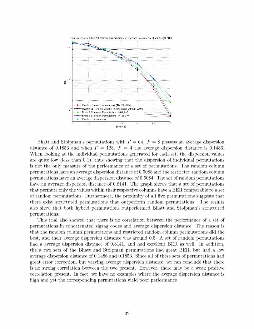
Bhatt and Stolpman’s permutations with I ′ = 64, J ′ = 8 possess an average dispersiondistance of 0.1853 and when I ′ = 128, J ′ = 4 the average dispersion distance is 0.1486.When looking at the individual permutations generated for each set, the dispersion valuesare quite low (less than 0.1), thus showing that the dispersion of individual permutationsis not the only measure of the performance of a set of permutations. The random columnpermutations have an average dispersion distance of 0.5088 and the restricted random columnpermutations have an average dispersion distance of 0.5084. The set of random permutationshave an average dispersion distance of 0.8141. The graph shows that a set of permutationsthat permute only the values within their respective columns have a BER comparable to a setof random permutations. Furthermore, the proximity of all five permutations suggests thatthere exist structured permutations that outperform random permutations. The resultsalso show that both hybrid permutations outperformed Bhatt and Stolpman’s structuredpermutations.

This trial also showed that there is no correlation between the performance of a set ofpermutations in concatenated zigzag codes and average dispersion distance. The reason isthat the random column permutations and restricted random column permutations did thebest, and their average dispersion distance was around 0.5. A set of random permutationshad a average dispersion distance of 0.8141, and had excellent BER as well. In addition,the a two sets of the Bhatt and Stolpman permutations had great BER, but had a lowaverage dispersion distance of 0.1486 and 0.1853. Since all of these sets of permutations hadgreat error correction, but varying average dispersion distance, we can conclude that thereis no strong correlation between the two present. However, there may be a weak positivecorrelation present. In fact, we have no examples where the average dispersion distance ishigh and yet the corresponding permutations yield poor performance

32

7 Future Work

In further studies, we would like to determine if variance is an accurate predictor of theerror-correcting capabilities of set permutations. If variance is not an accurate predictor,we would like to find another predictor for sets of permutations. In addition, we hope todetermine if the average dispersion of the permutations of Sn approaches a constant around0.81 as n increases and if that value can be written in terms of common constants or a sumof a known sequence. To aid in future simulations, we would like to improve the efficiencyof the zigzag simulator by either streamlining the Matlab code or implementing a version inC++. We would also like to include frame error rates, the amount of uncorrectable framesto the total number of frames transmitted. Finally, we would like to run more simulationsusing random column permutations versus random permutations.

33

8 Acknowledgements

This research was conducted at the Applied Mathematical Sciences Summer Institute (AMSSI)and has been partially supported by grants given by the Department of Defense (through itsASSURE program), the National Science Foundation (DMS-0453602), and National Secu-rity Agency (MSPF-07IC-043). Substantial financial and moral support was also providedby Don Straney, Dean of the College of Science at California State Polytechnic University,Pomona. Additional financial and moral support was provided by the Department of Math-ematics at Loyola Marymount University and the Department of Mathematics & Statisticsat California State Polytechnic University, Pomona. The authors are solely responsible forthe views and opinions expressed in this research; it does not necessarily reflect the ideasand/or opinions of the funding agencies and/or Loyola Marymount University or CaliforniaState Polytechnic University, Pomona.

We would also like to thank Dr. Edward Mosteig for spending his summer with us. Wewish him well for all his future endeavors. We would like to thank Laura Smith for all of heradvice and compassion. We would like to thank David Uminsky for being awesome. Finally,we would like to thank the directors, Dr. Erika Camacho and Dr. Stephen Wirkus, the otherfaculty, Dr. Lily Khadjavi and Dr. Angela Gallegos, and everyone else who made AMSSIpossible. Thanks for a great summer.

34

9 Programs

This section documents the Matlab code and the C++ code used throughout this project.

9.1 Zigzagsimualator

This program is the main function that calls upon all the other subfunctions to calculateBERs for given SNRs and Permutations. The user sends it the dimensions of the messagethey would like to produce.

function BER = Zigzagsimulator2(I,J,SNR,PI,NUMITERS) %%

%%%%%%%%%%%%%%%%%%%%%%%%%%%%%%%%%%%%%%%%%%%%%%%%%%%%%%%%%%%

% Zigzag Code Used to Simulate BER %

% The second draft of the main function that relies on %

% user input for the dimensions of the message, I, J, %

% a vector of values for the SNR, Pi for the Permutations,%

% and the number of iterations the decoder will go though %

% created: July 2, 2007 %

% modified: July 9, 2007 %

% Applied Mathematical Science Institute %

% Team Special Ed %

%%%%%%%%%%%%%%%%%%%%%%%%%%%%%%%%%%%%%%%%%%%%%%%%%%%%%%%%%%%

diary ’BERexecute.txt’; %%

%1.) Declaration of Variables

NUMERRORS = 500; % Tolerance of Errors

BER = zeros(1,length(SNR)); % initialization of Bit-Error-Rate

FRAME = zeros(1,length(SNR));

[K x] = size(PI); % determines how many subiterations

BLOCKLENGTH = I*(J); % The number of bits for each codeword

fprintf(’ === Variables Declared === \n’); %%

%2.) Main loop: runs the whole simulation for

% each value of snr placed in the SNR array

fprintf(’ === Loop Started === \n’) for s=1:length(SNR)

loops = 0; % initializes loop count at 0

errors = 0; % initializes error count at 0 for each pass through

frameerror = 0; % initializes frame error count to 0

IP = zeros(K,I*J); % loop used to determine the inverse permutation

for k=1:K % for each of the K permutations

IP(k,PI(k,:)) = 1:I*J;

end

while(errors < NUMERRORS)% when the number of errors is greater than our

% allowed limit the loop ends

D = RandMessage(I,J);% randomly generates a message

35

%%% ENCODING BEGINS

P = Parities(D,PI); % calculates the parities for each permutation

C = codeword(D,P); % merges D and P into a 1xI*(J+K) vector

C = tilde(C); % maps 0->1 and 1->(-1)

%%% ENCODING ENDS

%%% SIMULATION OF ERRORS BEING INTRODUCED

% USING GAUSSIAN NOISE

[R, sigma] = whitenoise(C,SNR(s),I*J, I*(J+K)); % R is the received word

%R = C; %<-Check’s encoding scheme-test for the DECODING

%%% END SIMULATION OF NOISEY CHANNEL

%%% DECODING BEGINS

Dtilde = R(1:I*J); % separates the received message bits from

% the received word

Ptilde = R(I*J+1:I*(J+K)); % separates the parity bits for each permutation

% from the received word

% the loops talk to eachother....sup?...nothing much you?...same

% old...how about those 1’s and -1’s?...O, they are ok, but they are

% a bit different from yours...O, really? How about I use some of

% yours...sure...

received = sign(Decode(PI,IP,I,J,K,Dtilde,Ptilde,NUMITERS,sigma));

% only concerned with whether the or not if the sign is positive or

% negative

% sums the errors from the decoded message to the original

errors = errors + sum(abs(C(1:I*J) - received))/2;

if errors~=0

frameerror = frameerror+1;

end

%errors = sum(abs(C - sign(R)))

loops = loops + 1; % increments the loop

end

BER(s) = errors/(loops*BLOCKLENGTH); %calculates the Bit Error Rate

fprintf(’\n’);

fprintf(’%s%1.2f%s%1.10f’,’For SNR = ’,SNR(s),’ the BER is ’, BER(s));

fprintf(’\n’);

end %%

% Graphs the different Bit Error Rates for the different SNR

ZigzagBERgraph(SNR,BER);

diary off;

36

9.1.1 RandMessage.m

%%%%%%%%%%%%%%%%%%%%%%%%%%%%%%%%%%%%%%%%%%%%%%%%%%%%%%%%%%%

% RandMessage.m %

% Creates a IxJ Random Message %


% %

% Applied Mathematical Science Institute 2007 %

% Team Special Ed %

%%%%%%%%%%%%%%%%%%%%%%%%%%%%%%%%%%%%%%%%%%%%%%%%%%%%%%%%%%%

function D = RandMessage(I,J)

D = zeros(I,J); % create a I x J matirx of zeros

for i=1:I

for j=1:J

if rand <= .5 % if rand is less than .5

D(i,j) = 1; % replace the d(i,j) with

end % with a 1

end

end

9.1.2 Parities.m

%%%%%%%%%%%%%%%%%%%%%%%%%%%%%%%%%%%%%%%%%%%%%%%%%%%%%%%%%%%

% Parities.m %

% Function used to compute the parities for each PI %


% %


% Team Special Ed %

%%%%%%%%%%%%%%%%%%%%%%%%%%%%%%%%%%%%%%%%%%%%%%%%%%%%%%%%%%%

% Function used to compute the parities for each Pi for D

function P = Parities(D,Pi)

[K IJ] = size(Pi);

for k=1:K

Temp = Permute(D,Pi(k,:));

P(k,:) = CalcParities(Temp);

end

37

9.2 Permute.m

%%%%%%%%%%%%%%%%%%%%%%%%%%%%%%%%%%%%%%%%%%%%%%%%%%%%%%%%%%%

% Permute.m %



% Team Special Ed %

%%%%%%%%%%%%%%%%%%%%%%%%%%%%%%%%%%%%%%%%%%%%%%%%%%%%%%%%%%%

function dk = Permute(D,Pi)

%%%%%%%%%%%%%%%%%%%%%

% this is how we permute

% pi = [3 4 5 2 6 1]

%(a1 a2 a3 a4 a5 a6)

% pi(a) = (a6 a4 a1 a2 a3 a5)

[I J] = size(D);

k = J;

for i=1:I

d(k-J+1:k) = D(i,:);

k = k +J;

end temp = d(Pi);

k=1;

for i=1:I

for j=1:J

dk(i,j) = temp(k);

k = k+1;

end

end

38

9.2.1 codeword.m

%%%%%%%%%%%%%%%%%%%%%%%%%%%%%%%%%%%%%%%%%%%%%%%%%%%%%%%%%%%

% Codeword.m %

% Function used to create the codeword sent through the %

% noisey channel %


% %


% Team Special Ed %

%%%%%%%%%%%%%%%%%%%%%%%%%%%%%%%%%%%%%%%%%%%%%%%%%%%%%%%%%%%

function c = codeword(D,P)

% D is the message

% P are the parities

% Returns 1*IJ+IK codeword

[I J] = size(D); [K IJ] = size(P);

d = reshape(D’, 1, I*J); p = reshape(P’, 1, K*IJ);

c = [d p];

9.2.2 tilde.m

%%%%%%%%%%%%%%%%%%%%%%%%%%%%%%%%%%%%%%%%%%%%%%%%%%%%%%%%%%%

% tilde.m %

% Function used to modulate the matrix to 1’s, and -1’s %

% from the original codeword of 0’s and 1’s %


% %


% Team Special Ed %

%%%%%%%%%%%%%%%%%%%%%%%%%%%%%%%%%%%%%%%%%%%%%%%%%%%%%%%%%%%

function modc = tilde(c)

modc = (-1).^c; %converts 1’s to -1’s and 0’s to 1’s

39

9.2.3 whitenoise.m

%%%%%%%%%%%%%%%%%%%%%%%%%%%%%%%%%%%%%%%%%%%%%%%%%%%%%%%%%%%

% whitenoise.m %

% Function used to simulate Gaussian white noise %

% and corrupts bits sent from the codeword %


% %


% Team Special Ed %

%%%%%%%%%%%%%%%%%%%%%%%%%%%%%%%%%%%%%%%%%%%%%%%%%%%%%%%%%%%

function [r sigma] = whitenoise(c, snr, k, n)

% c: codeword

% snr: signal to noise ratio

% k/n is the rate

% returns sigma and the distorted vector

en = 10 ^(snr/10); sigma = 1/(sqrt(2*en*(k/n))); r = c; for

i=1:length(c)

x = rand();

if x < 10^(-50)

x = 10^(-50);

end

r(i) = c(i)+ sigma*sqrt(-2*log(x))*cos(2*pi*rand());

end

9.2.4 Decode.m

%%%%%%%%%%%%%%%%%%%%%%%%%%%%%%%%%%%%%%%%%%%%%%%%%%%%%%%%%%%

% Decode.m %

% Function that decodes the received codeword %


% %


% Team Special Ed %

%%%%%%%%%%%%%%%%%%%%%%%%%%%%%%%%%%%%%%%%%%%%%%%%%%%%%%%%%%%

function Final = Decode(Pi,iP,I,J,K,Dtilde,Ptilde,numiters,sigma)

Le = zeros(K,I*J); Lo = zeros(1,I*J);

for iter=1:numiters

for k=1:K

Le(k,:) = calcLe(Ptilde((k*I-I+1):(k*I)),Pi(k,:),iP(k,:),Lo,I,J);

clip(Le);

Lo = calcLo(Dtilde,Le,k,K,Pi(k,:));

40

clip(Lo);

end

end Final = FinalLLR(Dtilde,Le,K);

9.2.5 calcLe.m

%%%%%%%%%%%%%%%%%%%%%%%%%%%%%%%%%%%%%%%%%%%%%%%%%%%%%%%%%%%

% calcLe.m %


% a function that computes part of extrinsic Information %

% on data bits %


% Team Special Ed %

%%%%%%%%%%%%%%%%%%%%%%%%%%%%%%%%%%%%%%%%%%%%%%%%%%%%%%%%%%%

function Le = calcLe(Ptilde,Pi,iP,Lo,I,J)

Lo = Permute(Lo,Pi); F = calcF(Ptilde,Lo,I,J); B =

calcB(Ptilde,Lo,I,J);

for j=1:J

temp = Lo(1:J);

temp(j) = Inf;

Le(j) = calcW([temp B(1)]);

end

for i=2:I

for j=1:J

temp = Lo(i*J-J+1:i*J);

temp(j) = Inf;

Le((i-1)*J+j) = calcW([temp B(i) F(i-1)]);

end

end Le = Permute(Le, iP);

41

9.2.6 calcF.m

%%%%%%%%%%%%%%%%%%%%%%%%%%%%%%%%%%%%%%%%%%%%%%%%%%%%%%%%%%%

% calcF.m %



% Team Special Ed %

%%%%%%%%%%%%%%%%%%%%%%%%%%%%%%%%%%%%%%%%%%%%%%%%%%%%%%%%%%%

function F = calcF(Ptilde,Lo,I,J)

%calcF

%a function that computes that forward recursion

%06/28/07

F(1) = Ptilde(1) + calcW([Inf Lo(1:J)]);

for i=2:I

F(i) = Ptilde(i) + calcW([F(i-1) Lo((i-1)*J+1:i*J)]);

end

9.2.7 calcB.m

%%%%%%%%%%%%%%%%%%%%%%%%%%%%%%%%%%%%%%%%%%%%%%%%%%%%%%%%%%%

% calcB.m %



% Team Special Ed %

%%%%%%%%%%%%%%%%%%%%%%%%%%%%%%%%%%%%%%%%%%%%%%%%%%%%%%%%%%%

function B = calcB(Ptilde,Lo,I,J)

%a function that computes that backward recursion

B(I) = Ptilde(I); for i=I:-1:2

B(i-1) = Ptilde(i-1) + calcW([B(i) Lo((i-1)*J+1:i*J)]);

end

42

9.2.8 calcW.m

%%%%%%%%%%%%%%%%%%%%%%%%%%%%%%%%%%%%%%%%%%%%%%%%%%%%%%%%%%%

% calcW.m %



% Team Special Ed %

%%%%%%%%%%%%%%%%%%%%%%%%%%%%%%%%%%%%%%%%%%%%%%%%%%%%%%%%%%%

function W = calcW(a)

% function that computes W

n = length(a);

tally = 1; min = inf;

for i=1:n

tally = tally * a(i);

if abs(a(i))<min

min = abs(a(i));

end

end

if tally < 0

sign = -1;

elseif tally > 0

sign = 1;

else

sign = 0;

end

W = sign*min;

9.2.9 calcLo.m

%%%%%%%%%%%%%%%%%%%%%%%%%%%%%%%%%%%%%%%%%%%%%%%%%%%%%%%%%%%

% calcLo.m %

% Function that decodes the received codeword %


% a function that computes part of extrinsic Information %

% on data bits %


% Team Special Ed %

%%%%%%%%%%%%%%%%%%%%%%%%%%%%%%%%%%%%%%%%%%%%%%%%%%%%%%%%%%%

function Lo = calcLo(Dtilde,Le,k,K,Pi)

[m n] = size(Le); sum = zeros(1,n);

43

for i=1:K

if i ~= k

sum = Le(i,:)+ sum;

end

end Lo = Dtilde + sum;

9.2.10 clip.m

%%%%%%%%%%%%%%%%%%%%%%%%%%%%%%%%%%%%%%%%%%%%%%%%%%%%%%%%%%%

% clip.m %



% Team Special Ed %

%%%%%%%%%%%%%%%%%%%%%%%%%%%%%%%%%%%%%%%%%%%%%%%%%%%%%%%%%%%

% Function that ensures that NaN is not ever a problem

% clips code and keeps it under control

function C = clip(m) [x y] = size(m);

B = ones(x,y)*10^7;

C = sign(m).*min(abs(m),B);

9.2.11 FinalLLR.m

%%%%%%%%%%%%%%%%%%%%%%%%%%%%%%%%%%%%%%%%%%%%%%%%%%%%%%%%%%%

% FinalLLR.m %



% Team Special Ed %

%%%%%%%%%%%%%%%%%%%%%%%%%%%%%%%%%%%%%%%%%%%%%%%%%%%%%%%%%%%

function Final = FinalLLR(Dtilde,Le,K)

% Takes Dtilde and the Le and makes the final decision on what the message was

[m n] = size(Le); sum = zeros(1,n); Final = zeros(n); for k=1:K

sum = Le(k,:) + sum;

end Final = sum + Dtilde;

44

9.3 Permutations

This section documents the codes of the various permutations used in our research.

9.3.1 Right to Left/Top to Bottom

Reads the matrix from right to left, top to bottom as the permutation.

%%%%%%%%%%%%%%%%%%%%%%%%%%%%%%%%%%%%%%%%%%%%%%%%%%%%%%%%%%%

% RLTB.m %

% Right to Left/Top to Bottom Classical Block Permutation %

% %


% Team Special Ed %

%%%%%%%%%%%%%%%%%%%%%%%%%%%%%%%%%%%%%%%%%%%%%%%%%%%%%%%%%%%

function temp = RLTB(M) [m n] = size(M); x = 1; y = n;

% Reads the matrix Right to Left/Top to Bottom as the Permutation

for i=1:m

for j=1:n

temp(i,j) = M(x,y);

x = x+1;

if x > m

x = 1;

y = y-1;

end

end

end

9.3.2 Right to Left/Bottom to Top

Reads the matrix from right to left, bottom to top as the permutation.

%%%%%%%%%%%%%%%%%%%%%%%%%%%%%%%%%%%%%%%%%%%%%%%%%%%%%%%%%%%

% RLBT.m %

% Right to Left/Bottom to Top Classical Block Permutation %

% %


% Team Special Ed %

%%%%%%%%%%%%%%%%%%%%%%%%%%%%%%%%%%%%%%%%%%%%%%%%%%%%%%%%%%%

function temp = RLBT(M) [m n] = size(M); x = m; y = n;

% Reads the matrix Right to Left/Bottom to Top as the Permutation

for i=1:m

for j=1:n

temp(i,j) = M(x,y);

x = x-1;

if x <= 0

45

x = m;

y = y-1;

end

end

end

9.3.3 Left to Right/Top to Bottom

Reads the matrix from left to right, top to bottom as the permutation.

%%%%%%%%%%%%%%%%%%%%%%%%%%%%%%%%%%%%%%%%%%%%%%%%%%%%%%%%%%%

% LRTB.m %

% Left to Right/Top to Bottom Classical Block Permutation %

% %


% Team Special Ed %

%%%%%%%%%%%%%%%%%%%%%%%%%%%%%%%%%%%%%%%%%%%%%%%%%%%%%%%%%%%

function temp = LRTB(M) [m n] = size(M) x = 1; y = 1;

% Reads the matrix Left to Right/Top to Bottom as the Permutation

for i=1:m

for j=1:n

temp(i,j) = M(x,y);

x = x+1;

if x > m

x = 1;

y = y+1;

end

end

end

9.3.4 Left to Right/Bottom to Top

Reads the matrix from left to right, bottom to top as the permutation.

%%%%%%%%%%%%%%%%%%%%%%%%%%%%%%%%%%%%%%%%%%%%%%%%%%%%%%%%%%%

% LRBT.m %

% Left to Right/Bottom to Top Classical Block Permutation %

% %


% Team Special Ed %

%%%%%%%%%%%%%%%%%%%%%%%%%%%%%%%%%%%%%%%%%%%%%%%%%%%%%%%%%%%

function temp = LRBT(M) [m n] = size(M) x = m; y = 1;

% Reads the matrix Left to Right/Bottom to Top as the Permutation

for i=1:m

for j=1:n

46

temp(i,j) = M(x,y);

x = x-1;

if x <= 0

x = m;

y = y+1;

end

end

end

9.3.5 Permutation Presented by Tejas Bhatt and Victor Stolpman

This code models the structured permutation presented by Tejas Bhatt and Victor Stolpman.

%%%%%%%%%%%%%%%%%%%%%%%%%%%%%%%%%%%%%%%%%%%%%%%%%%%%%%%%%%%

% BhattPermutation.m %

% July 16, 2007 %


% Team Special Ed %

%%%%%%%%%%%%%%%%%%%%%%%%%%%%%%%%%%%%%%%%%%%%%%%%%%%%%%%%%%%

function Mat = BhattPermutation(I,J,K, PrimeI, PrimeJ)

% model of the permutation presented

% by Tejas Bhatt and Victor Stolpman in ’Structured

% Interleavers and Decoder Architectures for Zigzag Codes’

% and in the US patent US 2007/0067697Al

% I,J: Block Length of the message

% K: number of permutations

% PrimeI, PrimeJ: the new shape of the matrix to use for permuting the IxJ

% matrix.

counter = 1; for i=1:PrimeI

for j=1:PrimeJ

M(i,j) = counter;

counter = counter+1;

end

end

%% Finding p’s

counter = 1; for i=1:I

if gcd(i,I)==1

p(counter) = i;

counter = counter + 1;

end

end

%% Find SjK

bool = 0; ind = 0; maxind =length(p);

47

% find the first prime number

while (bool == 0 && ind < maxind)

ind = ind + 1;

v = 1:PrimeJ;

S(1,:) = mod(v.*p(ind),PrimeI);

bool = conditionA(S(1,:));

end if ind == maxind

tempM = ’ERROR-out of prime numbers’;

return

end

% find K-1 more prime numbers

if K>1

for k=2:K

bool1 = 0;

bool2 = 0;

while(bool1==0 && bool2==0 && ind < maxind)

ind = ind + 1;

v = 1:PrimeJ;

S(k,:) = mod(v.*(ind),PrimeI);

% make sure that there is no repeated Sk values

bool1 = conditionA(S(k,:));

j = 1;

while(j<=length(S)&&bool==0)

% makes sure that there will be no bits in the same parity more than once

bool2 = conditionB(S(k,:),S(j,:));

j = j+1;

end

if ind == maxind

tempM = ’ERROR-out of prime numbers’;

return

end

end

end

end

%% Perform Column Shift--yo

%temp = reshape(M’,PrimeI,PrimeJ);

for k=1:K

for j=1:PrimeJ

temp(:,j,k) = circshift(M(:,j),S(k,j));

end

end

%% Bit-reversing

[Y,Mult] = bitrevorder([1:PrimeI]); for i=1:PrimeI

temp2(i,:,:) = temp(Mult(i),:,:);

end

48

%% Flatten the matrix----raaaaaaaaawwwwwwwrrrr---big dino feet!

for k=1:K

tempM(:,:,k) = reshape(temp2(:,:,k)’,1,I*J);

end

%% Make it a better format

Mat = un3d(tempM);

9.3.6 conditionA.m

%%%%%%%%%%%%%%%%%%%%%%%%%%%%%%%%%%%%%%%%%%%%%%%%%%%%%%%%%%%

% conditionA.m %

% July 16, 2007 %


% Team Special Ed %

%%%%%%%%%%%%%%%%%%%%%%%%%%%%%%%%%%%%%%%%%%%%%%%%%%%%%%%%%%%

function bool = conditionA(v)

% takes a vector and makes sure there are no repeated values in the vector

bool = 1; for i=1:length(v)-1

for j=i+1:length(v)

if v(i) == v(j)

bool = 0;

end

end

end

9.3.7 conditionB.m

%%%%%%%%%%%%%%%%%%%%%%%%%%%%%%%%%%%%%%%%%%%%%%%%%%%%%%%%%%%

% conditionB.m %

% July 16, 2007 %


% Team Special Ed %

%%%%%%%%%%%%%%%%%%%%%%%%%%%%%%%%%%%%%%%%%%%%%%%%%%%%%%%%%%%

function bool = conditionB(v1,v2)

% checks and makes sure two infor bits will only act in the same column row

% once

bool = 0; for i=1:length(v1)-1

for j=i+1:length(v1)

if v1(i)-v1(j) == v2(i)-v2(j)

bool = 1;

end

end

end

49

9.3.8 un3d.m

%%%%%%%%%%%%%%%%%%%%%%%%%%%%%%%%%%%%%%%%%%%%%%%%%%%%%%%%%%%

% un3d.m %

% July 16, 2007 %


% Team Special Ed %

%%%%%%%%%%%%%%%%%%%%%%%%%%%%%%%%%%%%%%%%%%%%%%%%%%%%%%%%%%%

function Mat = un3d(v)

% resizes a 3D array into a 2D array

[I J K] = size(v); for k=1:K

Mat(k,:) = v(:,:,k);

end

9.3.9 Randomly Permuting Each Column

Function that randomly permutes each individual column of the matrix, not allowing thethe entries each column to leave their respective column.

%%%%%%%%%%%%%%%%%%%%%%%%%%%%%%%%%%%%%%%%%%%%%%%%%%%%%%%%%%%

% randcolperm.m %

% July 16, 2007 %


% Team Special Ed %

%%%%%%%%%%%%%%%%%%%%%%%%%%%%%%%%%%%%%%%%%%%%%%%%%%%%%%%%%%%

function [temp4 disp]= randcolperm(I,J,K)

% Randomly permutes values within a column for each column, no values are

% allowed to leave their respective column. It then returns a permutation.

%% Make General Matrix

M = zeros(I,J); counter = 1; for i=1:I

for j=1:J

M(i,j) = counter;


end

end

%% Start making K permutations

for k=1:K

%% Declare Random Permutations for Each Column j

for j=1:J

Pi(j,:) = randperm(I);

disp(k,j) = fastdisp(Pi(j,:));

end

%% Take the transpose of the matrix and Permute the matrix

temp1 = M’;

temp2 = M’;

for j=1:J

50

temp2(j,:) = Permute(temp1(j,:),Pi(j,:));

end

temp3 = temp2’;

%% Flatten the new Matrix

temp4(k,:) = reshape(temp3’,1,I*J);

end

9.3.10 Randomly Permute Each Column with a Restriction

Function that randomly permutes each individual column of the matrix, not allowing thethe entries each column to leave their respective column. The restriction is that rows cannot have the same two information bits in different permutations’ rows more than two times.

%%%%%%%%%%%%%%%%%%%%%%%%%%%%%%%%%%%%%%%%%%%%%%%%%%%%%%%%%%%

% restrictedrandcolperm.m %

% July 17, 2007 %


% Team Special Ed %

%%%%%%%%%%%%%%%%%%%%%%%%%%%%%%%%%%%%%%%%%%%%%%%%%%%%%%%%%%%

function perm= restrictedrandcolperm(I,J,K)

% Randomly permutes values within a column for each column, no values are

% allowed to leave their respective column. It then returns a permutation.

% makes sure no more than rows of each permutation has no more than two

% shared information bits.

%% Make General Matrix

M = zeros(I,J); counter = 1; for i=1:I

for j=1:J

M(i,j) = counter;


end

end

%% Start making K permutations

k = 1; while k<=K

%% Declare Random Permutations for Each Column j

for j=1:J

Pi(j,:) = randperm(I);

end

%% Take the transpose of the matrix and Permute the matrix

temp1 = M’;

temp2 = M’;

for j=1:J

temp2(j,:) = Permute(temp1(j,:),Pi(j,:));

end

temp3 = temp2’;

%% Determine if the no rows have repeat columns

51

if k~=1

bool = 1; %assume the permutation is good

kd = 0;

while(kd<k-1 && bool == 1)

kd = kd+1;

for t1 = 1:I

t2 = 0;

while(t2<I&&bool==1)

t2 = t2+1;

difference = temp3(t1,:)-storage(t2,:,kd);

counter = 0;

for t3=1:length(difference)

if difference(t3)==0

counter = counter+1;

end

end

if counter > 2

bool = 0;

end

end

end

end

if bool == 1

storage(:,:,k) = temp3(:,:);

k = k+1;

end

else

storage(:,:,k) = temp3(:,:);

k = k+1;

end

end perm = storage;

%% Flatten the matrix----raaaaaaaaawwwwwwwrrrr---big dino feet!

for k=1:K

tempM(:,:,k) = reshape(storage(:,:,k)’,1,I*J);

end

%% Make it a better format

perm = un3d(tempM);

52

9.3.11 swapperperm.m

%%%%%%%%%%%%%%%%%%%%%%%%%%%%%%%%%%%%%%%%%%%%%%%%%%%%%%%%%%%

% swapperperm.m %

% %


% Team Special Ed %

%%%%%%%%%%%%%%%%%%%%%%%%%%%%%%%%%%%%%%%%%%%%%%%%%%%%%%%%%%%

function result = swapperperm(v,K)

% takes a vector, and for every ten values the first five values of that

% block are switched with the last five values of the block. Same idea with

% the remainder if the block length is not an a factor of ten, but switches

% the last five values with the remaining values from the last block.

n = size(v);

r = mod(n(2),10); % find the remainder of the size

% divided by 10

j = 6; % initial value of 10

k = 0; % k is initially 1

for i=1:(n(2)-r) % look at the values up to the remainder

if j-k <= 10 % ensures the values are only swapped once

a(j) = v(i); % assign v(i)’s value to a temp variable

a(i) = v(j); % assign a(i)

j = j+1;

end

if mod(i,10) == 0% resets the process for each multiple of 10

k = k + 10;

j = 6 + k;

end

end

j = n(2) - r + 1; % parameters for dealing with the remainder

b = 0; % j is where the remainder starts

while j <= n(2)

a(j) = v(n(2)-b); %assigns value to array

j = j+1;

b = b+1;

end for k =1:K result(k,:)= a(1,:); end

9.3.12 Magic Square Permutation

Creates a Magic Square and returns the square as a row vector used as a permutation.

53

%%%%%%%%%%%%%%%%%%%%%%%%%%%%%%%%%%%%%%%%%%%%%%%%%%%%%%%%%%%

% magicsquareperm.m %

% %


% Team Special Ed %

%%%%%%%%%%%%%%%%%%%%%%%%%%%%%%%%%%%%%%%%%%%%%%%%%%%%%%%%%%%

function ft = magicsquareperm(n)

% a generates a n by n magic square and turn it into a 1 dimensional vector

% used as a permutaiton.

ft = zeros(1,n); v = magic(n);

%first start with a zero vector of length 1000000.

for j = 1:n

ft(n*j - (n-1):n*j)=v(j,:);

end;

9.3.13 throwupperm.m

%%%%%%%%%%%%%%%%%%%%%%%%%%%%%%%%%%%%%%%%%%%%%%%%%%%%%%%%%%%

% throwupperm.m %

% Dated: June 24, 2007 %


% Team Special Ed %

%%%%%%%%%%%%%%%%%%%%%%%%%%%%%%%%%%%%%%%%%%%%%%%%%%%%%%%%%%%

function T = throwupperm(N)

%given a random message throwupperm swaps the rows of a matrix bottom up so

%that we get diffrent parodies

[A B]= size(N) M = zeros(A,B) k=1 for i= 1:A

for j = 1:B

M(i,j) = k;

k = k+1;

end

end

T(1,:) = flatten(M);

k = 2; for i = A:-1:2

M = swaprows(M,i,1)

c = T(k-1,:) - flatten(M)

for i = 1: (ceil(mod(rand*10000,B)) + 2)

%pick a random row and shift it

54

w = (ceil(mod(rand*10000,A)))

x=M(w,:);

M(w,:)=horazontalswrill(x’);

%pick a random row and swril it

end

if find (c) ~= 0

T(k,:) = flatten(M); %turn it into a permutation

k=k+1;

end

end

9.3.14 flatten.m

%%%%%%%%%%%%%%%%%%%%%%%%%%%%%%%%%%%%%%%%%%%%%%%%%%%%%%%%%%%

% flatten.m %

% created: June 30, 2007 %


% Team Special Ed %

%%%%%%%%%%%%%%%%%%%%%%%%%%%%%%%%%%%%%%%%%%%%%%%%%%%%%%%%%%%

function T = flatten(M)

%takes a message and flattens it

[A B] = size(M)

T =reshape(M’, 1,A*B)

9.3.15 swapprows.m

%%%%%%%%%%%%%%%%%%%%%%%%%%%%%%%%%%%%%%%%%%%%%%%%%%%%%%%%%%%

% swapprows.m %



% Team Special Ed %

%%%%%%%%%%%%%%%%%%%%%%%%%%%%%%%%%%%%%%%%%%%%%%%%%%%%%%%%%%%

function r = swaprows(M, a, b)

% given a matrix M swaps rows a and b

temp(1,:) = M(a,:); M(a,:) = M(b,:); M(b,:) = temp(1,:); r =

M;

55

9.3.16 horazontalswrill.m

%%%%%%%%%%%%%%%%%%%%%%%%%%%%%%%%%%%%%%%%%%%%%%%%%%%%%%%%%%%

% horazontalswrill.m %



% Team Special Ed %

%%%%%%%%%%%%%%%%%%%%%%%%%%%%%%%%%%%%%%%%%%%%%%%%%%%%%%%%%%%

function T = horazontalswrill(n)

%takes a perumtation n and swirls it around by a random amount

[A B] = size(n)

c = ceil(mod(rand*rand*1000,B-1))

T = circshift(n,c);

9.4 Dispersion and their Measurements

9.4.1 sumvarows.m

This function calculates variance of a permutation.

%%%%%%%%%%%%%%%%%%%%%%%%%%%%%%%%%%%%%%%%%%%%%%%%%%%%%%%%%%%

% sumvarows.m %



% Team Special Ed %

%%%%%%%%%%%%%%%%%%%%%%%%%%%%%%%%%%%%%%%%%%%%%%%%%%%%%%%%%%%

function [varsum, T ] = sumvarows(m,rows,cols)

[A B] = size(m); % create said matrix

k=1; w = zeros(rows,cols); m(1,:); for a = 1:rows

for b = 1:cols

w(a,b) = (m(1,k)); %puts the elements of the permutation in the matrix

%as if they were apart of the identity function

k = k+1;

end

end

if (A> 1)

for t = 2:A

k = 1;

56

temp =zeros(rows,cols);

for a = 1:rows

for b = 1:cols

temp(a,b) = ceil(m(t,k)/cols);

k = k+1;

end

end

w = [w;temp]; %append the new matrix on top of the old one

end

end [Q U]= size(w);

for i = 1: Q

T1(i) = var(w(i,:)); %take the variance

T(i) = T1(i)*(U-1)/(U);%multiply by constat to turn it into population variance

end

9.4.2 dispoflistofpermswithinvers.m

%%%%%%%%%%%%%%%%%%%%%%%%%%%%%%%%%%%%%%%%%%%%%%%%%%%%%%%%%%%

% dispoflistofpermswithinvers.m %



% Team Special Ed %

%%%%%%%%%%%%%%%%%%%%%%%%%%%%%%%%%%%%%%%%%%%%%%%%%%%%%%%%%%%

function R = dispoflistofpermswithinverse(n)

%this function given a list of permutations

%computes the dispersion every permutations with the inverse

%of another permutation.

[A,B] = size(n); T=zeros(A,B);

for i = 1:A

for j = 1:B

if(j<i)

temp = compute2perms(n(i,:),inverseperm(n(j,:)));

%compute the values of the matrix

T(i,j)=fastdisp(temp(1,:));

end

end

end

R = sum(sum(T))/(A*(A-1)/2); %take the average

57

9.4.3 inverseperm.m

%%%%%%%%%%%%%%%%%%%%%%%%%%%%%%%%%%%%%%%%%%%%%%%%%%%%%%%%%%%

% inverseperm.m %



% Team Special Ed %

%%%%%%%%%%%%%%%%%%%%%%%%%%%%%%%%%%%%%%%%%%%%%%%%%%%%%%%%%%%

function IP = inverseperm(PI)

%computes the inverse perm

[A B] = size(PI);

IP = zeros(1,B); % loop used to determine the inverse permutation

IP(PI(1,:)) = 1:B;

9.4.4 compute2perms.m

%%%%%%%%%%%%%%%%%%%%%%%%%%%%%%%%%%%%%%%%%%%%%%%%%%%%%%%%%%%

% compute2perms.m %



% Team Special Ed %

%%%%%%%%%%%%%%%%%%%%%%%%%%%%%%%%%%%%%%%%%%%%%%%%%%%%%%%%%%%

function T = compute2perms(a,b)

%given two permutations of the same block length this function puts the

%identity through 1 permutation the the other

[A B] = size(a);

for i = 1:B

T(b(i)) = a(i);

end

58

9.5 Triangular Distance and Random Walks

This program uses Triangular Distance Equations generated by Random Walks along thenumber line from -n to n, defined by user input. Random Walks on the set(−n . . . −2 −1 0 1 2 . . . n

)produced more than the Triangular Distance tables

for the permutations on Sn. The program determines whether or not the steps taken bythe Random Walk are in fact a Triangular Distance, and prints out each solution and totalnumber of solutions. C++ was used due to the abstract data type Doubly Linked Lists andthe flexibility of this kind of data type.

/****************************************************/

/* Random Walks Using Linked Lists */

/* by */

/* Applied Mathematical Science Institute */

/* Team Special Ed */

/* created: 7/12/2007 */

/* modified: 7/12/2007 */

/* This program uses random walks under set */

/* conditions to generate all of the random */

/* permutations of the Symmetric Group n */

/* using Triangular Distance Tables */

/****************************************************/

#include <iomanip> #include <iostream> #include <fstream>

// Create a structure to store each point on

// the numberline.

struct Node {

int n,visit;

bool visited;

Node *Next,*Prev;

};

//FUNCTIONS

void initialize(); // initializes Head and Tail

Nodes void create(int sample); // creates the number line

from n void marknode(int n, bool value); // marks the specified

node true or false Node next(Node *temp, int step);

// moves to next node specified by step

Node prev(Node *temp, int step);

//moves to prev node specified by step

bool isaperm();

// verifies that a permutation was created

59

void search(Node *t, int max, int counter);

// searches for permutations

//GLOBAL VARIABLES

Node Head; // The top node represents 0 on

the number line Node Tail; // The tail node set to 1000000

// as "wall" between -n and n.

int *iter,*use; // pointers that correspond to

// the amount each step

// can be used.

int *diag; // pointer that corresponds to

// the steps or distances

// on the diagonal

int *visitednodes; // pointer that corresponds to

// the nodes visited

int *perm;

// pointer that corresponds with the permutation int solutions, sample;

// number of solutions and sample size respectively

using namespace std;

void initialize() {

Head.n = 0; // set Head equal to 0

Head.Next = Head.Prev = &Tail; // set the Head pointers to point to the Tail

Tail.Next = Tail.Prev = &Head; // set the Tail pointers to point to the Head

Tail.n = 1000000; // create a really tall "wall"

Tail.visited = true; // set Tail’s visited value to true--no one likes Tail

solutions = 0; // no solutions...yet

}

void create(int sample) {

Node *temp1,*temp2; // temp Node pointers

temp1 = &Head; // set temp1 to point at Head

int i; // loop variable

for(i=1;i<=sample;i++) // create the positive side of the number line

{

temp2 = new Node;

temp2->Next = temp1->Next;

temp1->Next->Prev = temp2;

temp1->Next = temp2;

temp2->Prev = temp1;

60

temp2->n = i;

temp2->visited = false;

temp2->visit = 0;

temp1 = temp2;

}

temp1 = &Head; // reset temp1 to point back at Head

for(i=1;i<=sample;i++) // create the negative side of the number line

{

temp2 = new Node;

temp2->Prev = temp1->Prev;

temp1->Prev->Next = temp2;

temp2->Next = temp1;

temp1->Prev = temp2;

temp2->n = (-1)*i;

temp2->visited = false;

temp2->visit = 0;

temp1 = temp2;

}

}

void marknode(int n, bool value) {

Node *temp;

temp = Tail.Prev;

while(temp->n!=n)

{

temp = temp->Next;

}

temp->visited = value;

if(value)

temp->visit += 1;

else

temp->visit -= 1;

}

Node next(Node *temp, int step) // where to start and how many

// "steps" forward

{

if(temp->n == 1000000) // make sure the "wall" isn’t climbed

{

return Tail;

}

int i;

Node *temp2;

temp2 = temp;

61

for(i=1;i<=step;i++) // "step" though each node

{

temp2 = temp2->Next;

if(temp2->n==1000000) // loop hit the "wall"

{

return Tail;

}

}

return *temp2; // return end point

}

Node prev(Node *temp, int step) // where to start and how many

// "steps" backwards

{

if(temp->n == 1000) // make sure the "wall" isn’t climbed

{

return Tail;

}

int i;

Node *temp2;

temp2 = temp;

for(i=1;i<=step;i++) // "step" though each loop

{

temp2 = temp2->Prev;

if(temp2->n==1000)

{

return Tail;

}

}

return *temp2; // return end point

}

bool isaperm()

{

int i; // i is the first number to use in the permutations

int ind; // navigator of the indexes of the pointer arrays

bool flag; // determines if permutation is found

for(i=1;i<=sample;i++) // start at one and go to n

{

ind = 1; // start at index 1 for diag and perm

flag = true; // initialize flag as true

perm[0] = i; // initialize first perm entry as i

while(flag)

{

perm[ind] = perm[ind-1] + diag[ind-1];

62

// determine the next entry using the corresponding diag entry and prev perm

// make sure perm value is within its limits

if(perm[ind] <= 0 || perm[ind]>sample)

flag = false;

if(ind==sample-1 && flag) // PERMUTATION FOUND!

{

return true;

}

ind++; // increment the index

}

}

return false; // no permutation found

}

void search(Node *t, int max, int counter) // recursion!

{

// takes a starting position, max steps and largest step and counter

if(counter == max) // took max amount of steps

{

if(abs(visitednodes[max-1]-visitednodes[0]) <= max && isaperm())

{

// two conditions needed to be meet: abs val of largest step can be no larger than the

// max step size and it must be a permutation

solutions++; // increase solutions counter

//print solution

cout << "\nSolution " << solutions << " is: " << "\nThe Diagonal is: ";

for(int i=0;i<=max-1;i++)

{

cout << diag[i] << " ";

}

cout << "\nThe Permutation is: ";

for(int j=0;j<=sample-1;j++)

{

cout << perm[j] << " ";

}

cout << "\nThe Nodes visited were: ";

for(int i=0;i<=max-1;i++)

{

cout << visitednodes[i] << " ";

}

cout << "\n";

}

return;

}

63

// start recursion

for(int i=1;i<=max;i++) // step sizes

{

if(use[i-1]+1<=iter[i-1])

{

use[i-1] += 1; // mark the node used one more time

marknode(t->n,true); // mark the node visited

Node *temp;

temp = &next(t,i);

if(temp->visited!=true) // if next node isn’t visited go to it

{

diag[counter] = i; // set diag to the i step value

visitednodes[counter] = temp->n; // mark visit

search(temp,max,counter+1); // recurse

}

temp = &prev(t,i);

if(temp->visited!=true)

{

diag[counter] = (-1)*i; // set diag to the i step value

visitednodes[counter] = temp->n; // mark visit

search(temp,max,counter+1); // recurse

}

marknode(t->n,false); // remark the node false--I was never there

use[i-1] -= 1; // take back of the use

}

}

}

void main() {

//ask for the set size and place it into sample

cout << "Please input the set size:";

cin >> sample;

initialize();

create(sample-1);

// create temp. arrays

iter = new int [sample-1];

use = new int [sample-1];

diag = new int [sample-1];

visitednodes = new int [sample-1];

perm = new int [sample];

// initialize the arrays

for(int i=0;i<=sample-1;i++)

{

iter[i] = abs((sample-1)-i);

use[i] = 0;

64

perm[i] = 0;

}

search(&Head,sample-1,0); // begin long search

// final output

cout << "\nThe number of solutions: " << solutions << "\n";

cout << "\n";

int x = 1;

Node temp2 = Head;

// message to prevent the program from closing at the end when running the

// executible file

cout << "\n\n Reached the end of the program.

Enter any character then ’Enter’ to exit: ";

cin >> x;

//delete arrays--deny all evidence of their existence

delete [] iter;

delete [] use;

delete [] diag;

delete [] visitednodes;

delete [] perm;

}

65

References

[Bh] Bhatt, Tejas; Stolpman, Victor. Structured Interleavers and Decoder Architectures forZigzag Codes, IEEE Conference Proceedings on Signals, Systems and Computers, Oct.-Nov. 2006, pp.99-104.

[Do] Dolloff, Jason; Kenz, Zackary; Rische, Jacquelyn; Rogers, Danielle Ashley; Smith,Laura; Mosteig, Edward. Algebraic Interleavers in Turbo Codes. California State Poly-technic University, Pomona and Loyola Marymount University.

[He] Heegard, Chris; Wicker, Stephen B. Turbo Coding, Kluwer Academic Publishers, USA,1999.

[Jo] Jones, Alaina; Moreno, Benjamin; Smith, Laura; Viteri, Andrea; Yao, Kouadio David;Mosteig, Edward. Exploring Interleavers in Turbo Coding, 2005 AMSSI Technical Report,available at www.amssi.org.

[Li] Little, John B.; Mosteig, Edward. Error Control Codes from Algebra and Geometry–Notes for SACNAS Minicourse, Oct. 2003.

[Tu] Tucker, Alan. Applied Combinatorics, 5 ed., Wiley, 2006.

[Pi(1)] Ping, Li; Chan, Sammy; Yeung, Kwan L. Iterative Decoding of Multi-DimensionalConcatenated Single Parity Check Codes, 1998 IEEE International Conference on Com-munications, vol. 1, pp. 131-135.

[Pi(2)] Ping, Li; Huang, Xiaoling; Phamdo, Nam. Zigzag Codes and Concatenated ZigzagCodes, IEEE Transactions on Information Theory, vol. 47, no. 2, Feb. 2001, pp. 800-807.

66

permutations in concatenated zigzag codesetcamach/amssi/reports/zigzag.pdfhigher rates correspond to...

Documents