permutation p-value approximation via generalized...
TRANSCRIPT

arXiv: arXiv:0000.0000
Permutation p-value approximation via
generalized Stolarsky invariance
Hera Y. He,
Stanford University
e-mail: [email protected]
Kinjal Basu,
e-mail: [email protected]
Qingyuan Zhao,
University of Pennsylvania
e-mail: [email protected]
Art B. Owen
Stanford University
e-mail: [email protected]
Abstract: It is common for genomic data analysis to use p-values from alarge number of permutation tests. The multiplicity of tests may requirevery tiny p-values in order to reject any null hypotheses and the com-mon practice of using randomly sampled permutations then becomes veryexpensive. We propose an inexpensive approximation to p-values for twosample linear test statistics, derived from Stolarsky’s invariance principle.The method creates a geometrically derived reference set of approximatep-values for each hypothesis. The average of that set is used as a pointestimate p and our generalization of the invariance principle allows us tocompute the variance of the p-values in that set. We find that in cases wherethe point estimate is small, the variance is a modest multiple of the squareof that point estimate, yielding a relative error property similar to thatof saddlepoint approximations. On a Parkinson’s disease data set, the newapproximation is faster and more accurate than the saddlepoint approx-imation. We also obtain a simple probabilistic explanation of Stolarsky’sinvariance principle.
1. Introduction
Permutation methods are commonly used to obtain p-values in genomic appli-cations, especially those involving gene sets. In even modestly large data sets,the exact permutation p-value becomes too expensive to compute. Then MonteCarlo sampling of random permutations becomes a standard approach. Genomicapplications often test thousands of hypotheses and then multiplicity adjustmentrequires that some small p-values be obtained if any null hypotheses are to be
1

He, Basu, Zhao & Owen/Stolarsky invariance for permutations 2
rejected. When p-values below ε are required to reject H0, then Knijnenburget al. (2009) recommend doing at least 10/ε random permutations. As a result,even Monte Carlo sampling for permutation tests can be prohibitively expen-sive, and hence it pays to search for fast approximations to the permutationp-value.
In this paper we develop rapidly computable approximations to some permu-tation p-values. The p-values we consider are for a difference in group means.The approximations are based on ideas from spherical geometry and discrepancy,related to the Stolarsky invariance principle (Stolarsky, 1973). As described be-low, the resulting approximations prove to be very accurate for the tiny p-valueswhere permutation methods are most difficult to use. The new approximationscome with a numerical estimate of their own accuracy. Although they are limitedto the two sample setting, that setting is very important in many applications.
We begin with some background on the genomic motivation of our work.Then we transition to spherical geometry. This section then gives an outline ofthe paper and a pointer to some software.
Genomic context
The specific problem that motivated us is testing for sets of genes associatedwith Parkinson’s disease (Larson and Owen, 2015). More details about this workare given in the first author’s dissertation (He, 2016). In these data sets, thereare m0 subjects without Parkinson’s disease and m1 subjects with it. One cantest whether Parkinson’s disease is associated with an individual gene by doinga t-test comparing gene expression levels in tissue samples from the two groupsof subjects. Biological interest is often summarized more by gene sets ratherthan individual genes. Gene sets have two advantages: small but consistentassociations of many genes with the test condition can raise power, and, thegene sets themselves often connect better to biological understanding than doindividual genes.
For gene set testing, we work with a null hypothesis where a variable of inter-est (here a binary disease status) is statistically independent of the expressionlevel of all the genes in the gene set. We will call the variable of interest a phe-notype, though it could be any binary variable such as treatment versus controlin an experiment. The most studied alternative hypotheses are those where thephenotype is associated with a location shift in some or all of the genes in agene set. Many test statistics, some quite elaborate, have been proposed for thisproblem. Ackermann and Strimmer (2009) have an extensive comparison of 261different gene set tests for this two sample setting. To cope with correlationsamong all of the genes within a gene set, testing is done through permutationsof the phenotype values with respect to the gene expression levels. They in-vestigated numerous ways that location shifts could manifest and judged teststatistics by the resulting power of permutation tests. In practice, one does notknow the precise form that the alternative will take. Fortunately, Ackermannand Strimmer (2009) identified two families of test statistics that performed wellacross their range of mean-shift scenarios.
He, Basu, Zhao & Owen/Stolarsky invariance for permutations 3
To describe the best test statistics, let tg be the ordinary t-statistic for asso-ciation of gene g’s expression level with a binary phenotype. It is a difference ofwithin-group means normalized by a standard error. Now let G be a set of genes.Ackermann and Strimmer (2009) found that linear and quadratic test statistics,LG =
∑g∈G tg and QG =
∑g∈G t
2g, yielded the most powerful permutation
tests, along with some simple approximations to those two statistics. These teststatistics were more effective than some substantially more complicated propos-als. Tian et al. (2005) use the test statistic LG/|G| where G is the cardinality ofG, and the JG score of Jiang and Gentleman (2007) is similar. The statistic LG,and approximations to it, did best when expression differences between the twoconditions tended to have the same sign for each g ∈ G. When many oppositelysigned treatment effects occurred, then QG and approximations to it did best.
In a permutation analysis, like Ackermann and Strimmer (2009) used, weconsider all N =
(nm1
)different ways to select a subset π containing m1 of the
n = m0 + m1 subjects. Let LπG be the linear test statistic recomputed as ifthose m1 subjects had been the affected group. Then one-sided and two-sidedpermutation p-values for LG are
p =1
N
∑π
1LπG>LG , and p =1
N
∑π
1|LπG|>|LG|,
respectively. Here 1E takes the value 1 if the event E occurs and zero otherwise.We also use 1(E) in places where we find it more readable than 1E . Under thenull hypothesis of independence, permutation tests derived from these p-valuesare exact by symmetry (Lehmann and Romano, 2005, Chapter 15.2). Note thatthe smallest possible value for p is 1/N which we call the granularity limit.
When N is too large for a permutation test to be computationally feasible,a standard practice is to estimate p via randomly sampled permutations ofthe treatment label, as proposed by Barnard (1963). We randomize the binarytreatment label M−1 times, letting π(`) be the affected group in randomization` for ` = 1, . . . ,M − 1. We let π(0) be the original allocation. Then the average
p =1
M
M−1∑`=0
1|Lπ(`)G |>|LG|
is used as an estimate of p (for the two-sided linear case). In this Monte Carlocomputation, the true permutation p-value p is the unknown parameter and pis the sample estimate of p. Note that p > 1/M because we have included theoriginal allocation in the numerator. Failure to include the original allocationπ(0) can lead to p = 0 which is very undesirable. Note that the Monte Carlogranularity limit 1/M can be much larger than the permutation limit 1/N . Whenp is quite small, an enormous number M of simulations may be required to getan accurate estimate of it. For instance, in genome wide association studies(GWAS), the customary threshold for significance is ε = 5 × 10⁻⁸, makingpermutation methods prohibitively expensive, or even infeasible. For a recentdiscussion of p-value thresholds in GWAS, see Fadista et al. (2016).
He, Basu, Zhao & Owen/Stolarsky invariance for permutations 4
In this paper, we work with an approximation to LG from Ackermann andStrimmer (2009). Let Xi = 1 if subject i is in condition 1 with Xi = 0 forcondition 0, and let Ygi be the expression level of gene g for subject i. Thesevariables have sample averages X and Yg respectively. Ackermann and Strimmer(2009) found that
∑g∈G
1
n
n∑i=1
Xi − XsX
Ygi − Ygsg
(1.1)
was in the same winning set of test statistics as LG, where sX and sg arestandard deviations of Xi and Ygi respectively.
To understand why the statistic in (1.1) performs similarly to LG, let ρgbe the sample correlation between Xi and Ygi. Then (1.1) is
∑g∈G ρg times
a constant (n − 1)/n that does not affect the permutation p-value. Now tg =√n− 2ρg/
√1− ρ2g and a Taylor approximation gives tg
.=√n− 2(ρg + ρ3g/2).
When many small correlations ρg contribute to the signal, then summing ρg asin (1.1) gives a test statistic that is almost equivalent to summing tg becauseeach ρ3g is then very small.
Let Yi = YGi ≡∑g∈G Ygi/sg, Y = (1/n)
∑ni=1 Yi and let 1n be a column
vector of n ones. Then we may rewrite (1.1) as
n∑i=1
Xi − X‖X − 1nX‖
Yi − Y‖Y − 1nY ‖
(1.2)
multiplied by a constant that only depends on n. Equation (1.2) describes a teststatistic that is a plain Euclidean inner product of two unit vectors x0,y0 ∈ Rn.Here x0 has i’th component (Xi − X)/‖X − 1nX‖ and y0 is similar.
There are N =(nm1
)distinct vectors found by permuting the entries in x0. We
label them x0,x1, . . . ,xN−1 with x0 being the original one. Letting ρ = xT0y0
we find that one and two-sided p-values for a linear statistic are
1
N
N−1∑k=0
1xTky0>ρ
and1
N
N−1∑k=0
1|xTky0|>|ρ| (1.3)
repectively. We prefer inferences based on two-sided tests, but it is simpler tostudy one-sided tests first and then translate the results to two-sided ones.
Spherical geometry
We are now ready to make a geometric interpretation. Let Sd = {z ∈ Rd+1 |zTz = 1} be the d-dimensional unit sphere. Our data x0,y0 are in a subsetof Sn−1 orthogonal to 1n. That subset is isomorphic to Sn−2 and so we workmostly with d = n−2. In our motivating setting, the vector x0 has m1 identicalpositive values and m0 identical negative values. The geometry here applies for

He, Basu, Zhao & Owen/Stolarsky invariance for permutations 5
an arbitrary unit vector x0, but we only develop practically usable tests forbinary x0.
For y ∈ Sd and t ∈ [−1, 1], the spherical cap of center y and height t isC(y; t) = {z ∈ Sd | 〈y, z〉 > t}, where 〈·, ·〉 is the usual Euclidean inner product.By symmetry, z ∈ C(y; t) if and only if y ∈ C(z; t). The one-sided linear p-value is the fraction of xk for 0 6 k < N that belong to C(y0; ρ). Viewingx0, . . . ,xN−1 as approximately uniformly distributed over Sd by symmetry it isthen natural to estimate p by
p1 = p1(ρ), where p1(t) ≡ vol(C(y0; t))
vol(Sd). (1.4)
We use spherical geometry to investigate the accuracy of the uniformity-basedestimate p1 from (1.4) and also to motivate sharper estimates.
Stolarsky’s invariance principal gives a remarkable description of the accuracyof p1. Points x0,x1, . . . ,xN−1 ∈ Sd have squared L2 spherical cap discrepancy
L22 = L2(x0, . . . ,xN−1)2 =
∫ 1
−1
∫Sd|p1(t)− p(z, t)|2 dσd(z) dt
where p(z, t) = (1/N)∑N−1k=0 1xk∈C(z,t) and σd is the uniform (Haar) measure
on Sd. Stolarsky (1973) shows that
dωdωd+1
× L22 =
∫Sd
∫Sd‖x− y‖dσd(x) dσd(y)− 1
N2
N−1∑k,`=0
‖xk − x`‖ (1.5)
where ωd is the (surface) volume of Sd. Equation (1.5) shows that the meansquared error of p1(t) as an estimate of the permutation p-value p(z, t) is deter-mined by the mean absolute Euclidean distances among the N points. In ourapplications, the N points will be the distinct permuted values of x0, but (1.5)holds for N arbitrary points xk ∈ Sd.
The left side of (1.5) is, up to normalization, a mean squared discrepancyover spherical caps. The mean of (p1− p)2 is taken over caps of all heights from−1 to 1 corresponding to p-values of all sizes between 0 and 1. It is not thena very good accuracy measure when p1(ρ) turns out to be very small, such as10−6. It would be more useful to get such a mean squared error taken over capsof exactly the size p1(ρ), and no others.
Brauchart and Dick (2013) consider quasi-Monte Carlo (QMC) sampling inthe sphere. They generalize Stolarsky’s discrepancy formula to include a weight-ing function on the height t. By specializing their formula, we get an expressionfor the mean of (p1 − p)2 over spherical caps of any fixed size. Discrepancytheory plays a prominent role in QMC (Niederreiter, 1992), which is about ap-proximating an integral by a sample average. The present setting is a reversalof QMC: the discrete average p over permutations is the exact value we seek,and the integral over a continuum is the approximation p. A second difference isthat the QMC literature focusses on choosing N points to minimize a criterionsuch as (1.5), whereas here the N points are determined by the problem.
He, Basu, Zhao & Owen/Stolarsky invariance for permutations 6
As we will show below, the estimate p1 is the average of p over all sphericalcaps C(y; ρ) under a uniform distribution on their centers, i.e., y ∼ U(Sd).Those caps have the same volume as C(y0; ρ). In addition to specializing tocaps C(y; t) with t = ρ we make a further refinement to caps whose centersy more closely resemble y0. We find that refining to y with yTx0 = yT
0x0 isespecially useful. Such y values have exactly the same linear test statistic thatthe observed data y0 had.
These restrictions on spherical caps impose the constraint y ∈ Y for someY ⊂ Sd. Then we can be sure that p(y0, ρ) 6 supy∈Y p(y, ρ). If we could computethis supremum, then we would have a conservative permutation p-value andbe sure of controlling type I errors. We are generally unable to compute thisquantity but we can find both E(p(y, ρ)) and Var(p(y, ρ)) under a referencedistribution y ∼ U(Y). Intuitively, taking Y ever closer to the ideal Y = {y0},should lead to a more accurate reference mean. The variance gives us a numericalmeasure of how accurate that reference mean is. The practical constraint on ourchoice of Y is that we must be able to compute these reference moments.
The first reference set is simply Y1 = Sd. Our refinement of this set isY2 = {y ∈ Sd | yTx0 = yT
0x0}. We obtain a computable expression forp2 = E(p(y, ρ)) and another one for E((p2−p(y, ρ))2), both under y ∼ U(Y2), byfurther extending Brauchart and Dick’s generalization of Stolarsky’s invariance.In principle we could refine Y2 further in the direction of {y0} by imposing ad-ditional linear constraints on y. For this paper we impose just one. Our proofsand algorithms work with the more general constraint yTxc = yT
0xc for anyc ∈ {0, 1, . . . , N − 1} that we like.
Our calculations show that√
Var(p2 − p(y, ρ)), for y ∼ U(Y2), does notgreatly exceed p2 when p2 is small and it even vanishes in the limit as p2 ↓ 1/N .The function p(y) is then nearly constant over y ∈ Y2 in this L2 sense, whichturns out to make p2 a much better estimate of p than p1 is. We cannot ruleout that the true p(y0) could be quite different from p2 for a data generatingprocess that differed in an adversarial way from the reference distribution, asdiscussed at the end of this article.
Although our results are mean square discrepancies via invariance, we canalso obtain them via probabilistic arguments. As a consequence we have a prob-abilistic derivation of Stolarsky’s formula. Bilyk et al. (2016) have independentlyfound this connection.
Outline
The rest of the paper is organized as follows. Section 2 presents some resultsfrom spherical geometry and defines our reference distributions. In Section 3 weuse Stolarsky’s invariance principle as generalized by Brauchart and Dick (2013)to obtain the mean squared error between the true p-value and its continuousapproximation p1, averaging over all spherical caps of volume p1. This sectionalso has a probabilistic derivation of that mean squared error. In Section 4we derive the refined estimate p2 and some generalizations. By construction
He, Basu, Zhao & Owen/Stolarsky invariance for permutations 7
p2 > 1/N , respecting the true granularity of permutation testing. In Section 5we modify the proof in Brauchart and Dick (2013), to further generalize theirinvariance results to include the mean squared error of p2. Section 6 extends ourestimates to two-sided testing. Section 7 illustrates our p-value approximationsnumerically. We see that the root mean squared error in the estimate p2 is of thesame order of magnitude as p2 itself. That is, p2 has a relative error propertylike saddlepoint estimates do. The estimate p1 is notably less accurate than p2.Section 8 makes a numerical comparison to saddlepoint methods in simulateddata. The saddlepoint estimates come out more accurate than p2 but are down-wardly biased in those simulated examples. Section 9 compares the accuracyof our approximations to each other and to the saddlepoint approximation for6180 gene sets in some Parkinson’s disease data sets. In the data examples, thenew approximations come out closer to some gold standard estimates (basedon large Monte Carlo samples) than the saddlepoint estimates do, which onceagain are biased low. From Table 6.3 of He (2016), the saddlepoint computationstake roughly 30 times longer than p2 does. Section 10 draws some conclusionsand discusses the challenges in getting a computationally feasible p-value thataccounts for both sampling uncertainty of the data and the uncertainty in pas an estimate of p. At several places we refer the reader to a supplement (Heet al., 2018) for additional material, including our lengthier proofs.
Software
The proposed approximations are implemented in the R package pipeGS onCRAN. Given a binary input label and a gene expression measurement matrix,it computes our p-value approximations for two sample problems. It includes thestatistics, p1 and p2 mentioned above as well as a saddlepoint approximationwhich may be of independent interest.
2. Background and notation
Here we develop approximations to the one-sided p-value in (1.3). That is simplerthan carrying the two-sided case through all of our derivations. We translatefrom one-sided to two-sided cases in Section 6.
The raw data contain points (Xi, Yi) for i = 1, . . . , n, where Yi may be acomposite quantity derived from all Ygi for g belonging to a gene set G, such asYi = YGi given just before (1.2). We center and scale vectors (X1, X2, . . . , Xn)and (Y1, Y2, . . . , Yn) yielding x0,y0 ∈ Sd for d = n − 1. Both points belong to{z ∈ Sn−1 | zT1n = 0}. We can use an orthogonal matrix to rotate the pointsof this set onto Sn−2 × {0}. As a result, we may simply work with x0,y0 ∈ Sdwhere d = n− 2.
The sample correlation of these variables is ρ = xT0y0 = 〈x0,y0〉. We use
〈x0,y0〉 when we find that geometrical thinking is appropriate and to conformwith Brauchart and Dick (2013). We use xT
0y0 to emphasize computational oralgebraic connotations.

He, Basu, Zhao & Owen/Stolarsky invariance for permutations 8
The geometry we use leads to practical algorithms when Xi takes on justtwo values, such as 0 and 1. When there are m0 observations with Xi = 0 andm1 with Xi = 1 then x0 contains m0 components equal to −
√m1/(nm0) and
m1 components equal to +√m0/(nm1). In our theorem statements we describe
such a point x0 as a “centered and scaled binary vector”.Computational costs are often sensitive to the smaller sample size, m ≡
min(m0,m1). For this two-sample case, there are only N =(m0+m1
m0
)distinct
permutations of x0. We have called these x0,x1, . . . ,xN−1 and the true p-value
is p = (1/N)∑N−1k=0 1(xT
ky0 > ρ) = (1/N)∑N−1k=0 1(xk ∈ C(y0; ρ)). In the two-
sample case we can define a useful interpoint swap distance
r = r(xk,x`) =
n∑i=1
1((xk)i > 0 & (x`)i < 0)
where (xk)i is the i’th component of xk. In the permutation taking xk onto x`there are r positive entries in xk that have been swapped with negative ones tocreate x`. In that case we easily find that
u(r) ≡ 〈xk,x`〉 = 1− r( 1
m0+
1
m1
). (2.1)
We need some geometric properties of the unit sphere and spherical caps. Thesurface volume of Sd is ωd = 2π(d+1)/2/Γ((d+1)/2). Recall that σd is the volumeelement in Sd normalized so that σd(Sd) = 1. Henceforth ‘volume’ will alwaysrefer to this normalized volume. The spherical cap C(y; t) = {z ∈ Sd | zTy > t}has volume
σd(C(y; t)) =
{12I1−t2
(d2 ,
12
), 0 6 t 6 1
1− 12I1−t2
(d2 ,
12
), −1 6 t < 0
where It(a, b) is the incomplete beta function
It(a, b) =1
B(a, b)
∫ t
0
xa−1(1− x)b−1 dx
with B(a, b) =∫ 1
0xa−1(1− x)b−1 dx.
We frequently need to use a tangent-normal decomposition (Mardia andJupp, 2000, Chapter 9.1). The tangent-normal decomposition of y with respectto x is
y = tx+√
1− t2y∗
where t = yTx ∈ [−1, 1] and y∗ ∈ {z ∈ Sd | zTx = 0} which is isomorphic toSd−1. The coordinates t and y∗ are unique. We refer to y∗ as the residual inthis decomposition. From equation (A.1) in Brauchart and Dick (2013)
dσd(y) =ωd−1ωd
(1− t2)d/2−1 dtdσd−1(y∗). (2.2)

He, Basu, Zhao & Owen/Stolarsky invariance for permutations 9
The intersection of two spherical caps of common height t is
C2(x,y; t) ≡ C(x; t) ∩ C(y; t).
We will need the volume of this intersection. Lee and Kim (2014) give a generalsolution for spherical cap intersections without requiring equal heights. Theyenumerate 25 cases, but our case does not correspond to any single case oftheirs and so we obtain the formula we need directly, below. We suspect it mustbe known already, but we were unable to find it in the literature.
Lemma 1. Let x,y ∈ Sd and −1 6 t 6 1 and put u = xTy. Let V2(u; t, d) =σd(C2(x,y; t)). If u = 1, then V2(u; t, d) = σd(C(x; t)). If −1 < u < 1, then
V2(u; t, d) =ωd−1ωd
∫ 1
t
(1− s2)d2−1σd−1(C(y∗; ρ(s))) ds, (2.3)
where ρ(s) = (t− su)/√
(1− s2)(1− u2). Finally, for u = −1,
V2(u; t, d) =
{0, t > 0ωd−1
ωd
∫ |t|−|t|(1− s
2)d2−1 ds, else.
(2.4)
Proof. See Section 11.1 of the supplement, He et al. (2018).
When we give probabilistic arguments and interpretations we do so for arandom center y of a spherical cap. That random center is taken from tworeference distributions given below. Reference distribution 1 is illustrated inFigure 1. Reference distribution 2 is illustrated in Figure 2 of Section 4 wherewe first use it.
Reference distribution 1. The vector y ∼ U(Y1) where Y1 = Sd. Expectationunder this distribution is denoted by E1(·).
Reference distribution 2. The vector y ∼ U(Y2) where
Y2 = Y2(c) = {z ∈ Sd | zTxc = ρ},
for some c ∈ {0, 1, . . . , N−1} and ρ = xTc y0. Then y = ρxc+
√1− ρ2y∗ for y∗
uniformly distributed on a subset of Sd isomorphic to Sd−1. Expectation underthis distribution is denoted by E2,c(·) and E2(·) means E2,0(·).
We also use Varj(·) for a variance under reference distribution j. Referencedistribution 1 holds for y0 if the Yi are IID Gaussian random variables (withpositive variance). Then p1 is the same as we would get from a t-test. Refer-ence distribution 2 is actually a family of reference distributions indexed by c.The choice of primary interest to us has c = 0 corresponding to the observedtreatment allocation. We write pc = E2,c(C(y; ρ)) and p2 = p0. This referencedistribution represents a significant narrowing of reference distribution 1. Wefind good numerical performance for p2 below.

He, Basu, Zhao & Owen/Stolarsky invariance for permutations 10
●
●
●
●
●
●
●
●
●●
●
●
●
●
●
●
●
●
●
●
●
●
●
●
●
●
●
●
●
●
●
●
●
●
●
●
●
●
●
●
●
●
●
●
●
●
●
●
●
●
●
●
●
●
●
●
●
●
●
●
●
●
●
●●
●
●
●
●
●
●
●
●
●
●
●
●
●
●
●
●●
●
●
●
●
●
●
●
●
●
●
●
●
●
●
●
●
●
●
●
●
●
●
●
●
●
●
●
●
●
●
●
●
●
●
●
●
●
●
●
●
●
●
●
●
●
●
●
●
●
●
●
●
●
●
●
●
●
●
●
●
●
●
●
●
●
●
●
●
●
●
●●
●
●
●
●
●
●
●
●
●
●
●
●
●
●
●
●
●
●
●
●
●
●
●
●
●
●
●
●
●
●
●
●
●
●
●
●
●
●
●
●
●
●
●
●
●
●
●
●
●
●
●
●
●
●
●
●
●
●
●
●
●
●
●
●
●
●
●
●
●
●
● ●
●
●
●
●
●
●
●
●
●
●
●
●
●
●
●
●
●
●
●
●
●
●
●
●
●
●
●
●
●
●
●
●
●
●
●
●
●
●
●
●
●
●
●
●
●
●
●
●
●
●
●
●
●
●
●
●
●
●
●
●
●
●
●
●
●
●
●
●
●
●
●●
●
●
●
●
●
●
●
●
●
●
●
●
●
●
●
●
●
●
●
●
●
●
●
●
●
●
●
●
●
●
●
●
●
●
●
●
●
●
●
●
●
●
●
●
●
●
●
●
●
●
●
●
●
●
●
●
●
●
●
●
●
●
●
●
●
●
●
●
●
●
●●
●
●
●
●
●
●
●
●
y0
●
y1
Sd
Fig 1: Reference distribution 1. Here y ∼ U(Sd) and y0 is the observed valueof y. The small open circles represent permuted vectors xk. The circle aroundy0 goes through x0 and represents a spherical cap of height ρ = yT
0x0. Asecond spherical cap of equal volume is centered at y1. We study moments ofthe permutation p-value p(y, ρ) for random y and fixed ρ.
3. Approximation via spherical cap volume
Here we study the approximate p-value p1(ρ) = σd(C(y; ρ)). First we find themean squared error of this approximation over all spherical caps of the givenvolume via invariance. Next we give a probabilistic interpretation which includesthe conditional unbiasedness result in Proposition 2 below. Then we give twocomputational simplifications, first taking advantage of the permutation struc-ture of our points, and then second for permutations of a centered and scaledbinary vector.
Brauchart and Dick (2013) gave a simple proof of Stolarsky’s invariance prin-ciple using reproducing kernel Hilbert spaces. They also generalized it as follows.
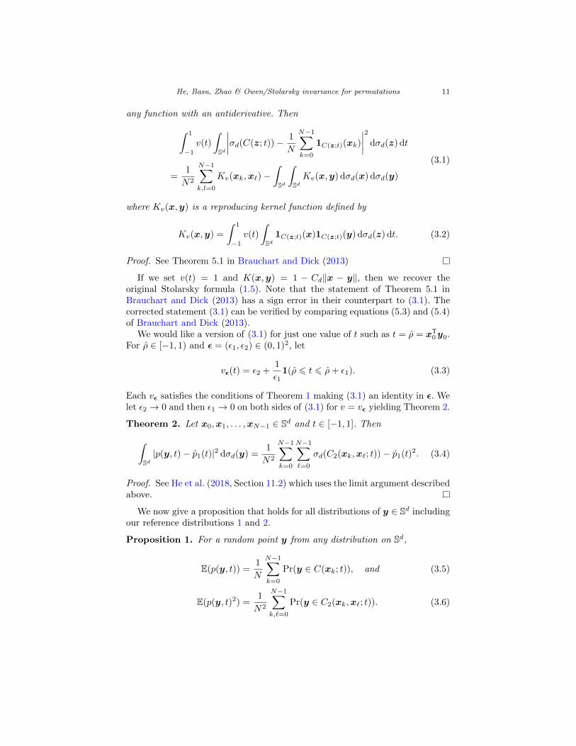
Theorem 1. Let x0, . . . ,xN−1 be any points in Sd. Let v : [−1, 1]→ (0,∞) be
He, Basu, Zhao & Owen/Stolarsky invariance for permutations 11
any function with an antiderivative. Then∫ 1
−1v(t)
∫Sd
∣∣∣∣σd(C(z; t))− 1
N
N−1∑k=0
1C(z;t)(xk)
∣∣∣∣2 dσd(z) dt
=1
N2
N−1∑k,l=0
Kv(xk,x`)−∫Sd
∫SdKv(x,y) dσd(x) dσd(y)
(3.1)
where Kv(x,y) is a reproducing kernel function defined by
Kv(x,y) =
∫ 1
−1v(t)
∫Sd
1C(z;t)(x)1C(z;t)(y) dσd(z) dt. (3.2)
Proof. See Theorem 5.1 in Brauchart and Dick (2013)
If we set v(t) = 1 and K(x,y) = 1 − Cd‖x − y‖, then we recover theoriginal Stolarsky formula (1.5). Note that the statement of Theorem 5.1 inBrauchart and Dick (2013) has a sign error in their counterpart to (3.1). Thecorrected statement (3.1) can be verified by comparing equations (5.3) and (5.4)of Brauchart and Dick (2013).
We would like a version of (3.1) for just one value of t such as t = ρ = xT0y0.
For ρ ∈ [−1, 1) and ε = (ε1, ε2) ∈ (0, 1)2, let
vε(t) = ε2 +1
ε11(ρ 6 t 6 ρ+ ε1). (3.3)
Each vε satisfies the conditions of Theorem 1 making (3.1) an identity in ε. Welet ε2 → 0 and then ε1 → 0 on both sides of (3.1) for v = vε yielding Theorem 2.
Theorem 2. Let x0,x1, . . . ,xN−1 ∈ Sd and t ∈ [−1, 1]. Then∫Sd|p(y, t)− p1(t)|2 dσd(y) =
1
N2
N−1∑k=0
N−1∑`=0
σd(C2(xk,x`; t))− p1(t)2. (3.4)
Proof. See He et al. (2018, Section 11.2) which uses the limit argument describedabove.
We now give a proposition that holds for all distributions of y ∈ Sd includingour reference distributions 1 and 2.
Proposition 1. For a random point y from any distribution on Sd,
E(p(y, t)) =1
N
N−1∑k=0
Pr(y ∈ C(xk; t)), and (3.5)
E(p(y, t)2) =1
N2
N−1∑k,`=0
Pr(y ∈ C2(xk,x`; t)). (3.6)

He, Basu, Zhao & Owen/Stolarsky invariance for permutations 12
Proof. These follow directly from p = (1/N)∑Nk=0 1(y ∈ C(xk; t)).
Proposition 2. For any x0, . . . ,xN−1 ∈ Sd and t ∈ [−1, 1],
E1(p(y, t)) = p1(t) and E1(p(y, t)2) =1
N2
N−1∑k=0
N−1∑`=0
σd(C2(xk,x`; t)).
Proof. We apply Proposition 1. Under reference distribution 1, each summandin (3.5) equals p1(t). Similarly the k, ` summand in (3.6) evaluates to σd(C2(xk,x`; t)).
Combining Proposition 2 with Theorem 2 we find that if y ∼ U(Sd), thenp(y, ρ) is a random variable with mean p1(ρ) and variance given by (3.4) witht = ρ. The right hand side of (3.4) sums O(N2) terms. The symmetry in apermutation set allows us to use∫
Sd|p(y, t)− p1(t)|2 dσd(y) =
1
N
N−1∑k=0
σd(C2(x0,xk; t))− p1(t)2
instead. This expression costs O(N), the same as the full permutation analysisthat we seek to avoid.
The cost becomes feasible when x0 is a centered and scaled binary vector.Then for fixed t, σd(C2(xk,x`; t)) just depends on the swap distance r betweenxk and x`. Let rk,` be the swap distance between xk and x` and let Nr =∑N−1k=0
∑N−1`=0 1(rk,` = r) count the number of point pairs at swap distance r.
Then ∫Sd|p(y, t)− p1(t)|2 dσd(y) =
1
N2
m∑r=0
NrV2(u(r); t, d)− p1(t)2 (3.7)
for V2(u(r); t, d) given in Lemma 1.
Theorem 3. Let x0 ∈ Sd be a centered and scaled binary vector with m0 > 1negative components and m1 > 1 positive components. Let x0,x1, . . . ,xN−1 bethe N =
(m0+m1
m0
)distinct permutations of x0. If y ∼ U(Sd), then for t ∈ [−1, 1],
and with u(r) defined in (2.1),
Var1(p(y, t)) =1
N
m∑r=0
(m0
r
)(m1
r
)V2(u(r); t, d)− p1(t)2, (3.8)
for V2(u(r); t, d) given in Lemma 1.
Proof. There are(m0
r
)(m1
r
)permuted points xk at swap distance r from x` for
each ` = 0, 1, . . . , N − 1. Therefore Nr = N(m0
r
)(m1
r
), establishing (3.8).
We will see in Section 7 that√
Var1(p(y, t))/E1(p(y, t)) becomes extremelylarge as t → 1 and E1(p(y, t)) → 0. Therefore extremely small spherical capvolumes are compatible with a wide range of permutation p-values.

He, Basu, Zhao & Owen/Stolarsky invariance for permutations 13
●
●
●
●
●
●
●
●
●●
●
●
●
●
●
●
●
●
●
●
●
●
●
●
●
●
●
●
●
●
●
●
●
●
●
●
●
●
●
●
●
●
●
●
●
●
●
●
●
●
●
●
●
●
●
●
●
●
●
●
●
●
●
●●
●
●
●
●
●
●
●
●
●
●
●
●
●
●
●
●●
●
●
●
●
●
●
●
●
●
●
●
●
●
●
●
●
●
●
●
●
●
●
●
●
●
●
●
●
●
●
●
●
●
●
●
●
●
●
●
●
●
●
●
●
●
●
●
●
●
●
●
●
●
●
●
●
●
●
●
●
●
●
●
●
●
●
●
●
●
●
●●
●
●
●
●
●
●
●
●
●
●
●
●
●
●
●
●
●
●
●
●
●
●
●
●
●
●
●
●
●
●
●
●
●
●
●
●
●
●
●
●
●
●
●
●
●
●
●
●
●
●
●
●
●
●
●
●
●
●
●
●
●
●
●
●
●
●
●
●
●
●
● ●
●
●
●
●
●
●
●
●
●
●
●
●
●
●
●
●
●
●
●
●
●
●
●
●
●
●
●
●
●
●
●
●
●
●
●
●
●
●
●
●
●
●
●
●
●
●
●
●
●
●
●
●
●
●
●
●
●
●
●
●
●
●
●
●
●
●
●
●
●
●
●●
●
●
●
●
●
●
●
●
●
●
●
●
●
●
●
●
●
●
●
●
●
●
●
●
●
●
●
●
●
●
●
●
●
●
●
●
●
●
●
●
●
●
●
●
●
●
●
●
●
●
●
●
●
●
●
●
●
●
●
●
●
●
●
●
●
●
●
●
●
●
●●
●
●
●
●
●
●
●
●
xc●
y0
●
y2●
y1
Sd
Fig 2: Reference distribution 2 with c = 0. The original response vector isy0 with yT
0x0 = ρ and x0 marked xc. We consider alternative y uniformlydistributed on the surface of C(x0; ρ) (dashed circle) with examples y1 and y2.Around each such yj there is a spherical cap of height ρ that just barely includesxc = x0. The small open circles are permutations xk of x0. The proportion ofxk ∈ C(y, ρ) is p(y, ρ). We study the mean and variance of p(y, ρ) for fixed ρand y ∼ U(Y2) for Y2 = {y ∈ Sd | yTx0 = ρ}.
4. A finer approximation to the p-value
In the previous section, we studied the distribution of permutation p-valuesp(y, t) with spherical cap centers y ∼ U(Sd) and heights t = ρ. In this section,we use reference distribution 2 to obtain a finer approximation to p(y0, ρ) bystudying the distribution of the p-values for centers y ∼ U(Y2(c)) for c ∈{0, 1, . . . , N−1}. For an index c ∈ {0, 1, . . . , N−1}, conditioning as above leadsto
pc = E2,c(p(y, ρ)) = E1(p(y, ρ) | yTxc = yT0xc), (4.1)
and our primary interest is in p2 = p0. For an illustration of reference distribu-tion 2 see Figure 2.
From Proposition 1, we can get our estimate pc and its mean squared error byfinding single and double inclusion probabilities for y. To compute pc we need
He, Basu, Zhao & Owen/Stolarsky invariance for permutations 14
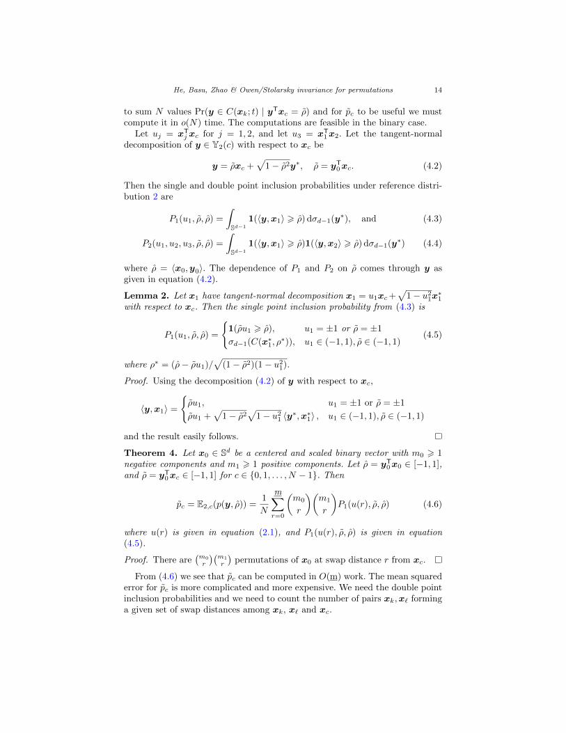
to sum N values Pr(y ∈ C(xk; t) | yTxc = ρ) and for pc to be useful we mustcompute it in o(N) time. The computations are feasible in the binary case.
Let uj = xTj xc for j = 1, 2, and let u3 = xT
1x2. Let the tangent-normaldecomposition of y ∈ Y2(c) with respect to xc be
y = ρxc +√
1− ρ2y∗, ρ = yT0xc. (4.2)
Then the single and double point inclusion probabilities under reference distri-bution 2 are
P1(u1, ρ, ρ) =
∫Sd−1
1(〈y,x1〉 > ρ) dσd−1(y∗), and (4.3)
P2(u1, u2, u3, ρ, ρ) =
∫Sd−1
1(〈y,x1〉 > ρ)1(〈y,x2〉 > ρ) dσd−1(y∗) (4.4)
where ρ = 〈x0,y0〉. The dependence of P1 and P2 on ρ comes through y asgiven in equation (4.2).
Lemma 2. Let x1 have tangent-normal decomposition x1 = u1xc+√
1− u21x∗1with respect to xc. Then the single point inclusion probability from (4.3) is
P1(u1, ρ, ρ) =
{1(ρu1 > ρ), u1 = ±1 or ρ = ±1
σd−1(C(x∗1, ρ∗)), u1 ∈ (−1, 1), ρ ∈ (−1, 1)
(4.5)
where ρ∗ = (ρ− ρu1)/√
(1− ρ2)(1− u21).
Proof. Using the decomposition (4.2) of y with respect to xc,
〈y,x1〉 =
{ρu1, u1 = ±1 or ρ = ±1
ρu1 +√
1− ρ2√
1− u21 〈y∗,x∗1〉 , u1 ∈ (−1, 1), ρ ∈ (−1, 1)
and the result easily follows.
Theorem 4. Let x0 ∈ Sd be a centered and scaled binary vector with m0 > 1negative components and m1 > 1 positive components. Let ρ = yT
0x0 ∈ [−1, 1],and ρ = yT
0xc ∈ [−1, 1] for c ∈ {0, 1, . . . , N − 1}. Then
pc = E2,c(p(y, ρ)) =1
N
m∑r=0
(m0
r
)(m1
r
)P1(u(r), ρ, ρ) (4.6)
where u(r) is given in equation (2.1), and P1(u(r), ρ, ρ) is given in equation(4.5).
Proof. There are(m0
r
)(m1
r
)permutations of x0 at swap distance r from xc.
From (4.6) we see that pc can be computed in O(m) work. The mean squarederror for pc is more complicated and more expensive. We need the double pointinclusion probabilities and we need to count the number of pairs xk,x` forminga given set of swap distances among xk, x` and xc.

He, Basu, Zhao & Owen/Stolarsky invariance for permutations 15
Lemma 3. For j = 1, 2, let rj be the swap distance of xj from xc and let r3 bethe swap distance between x1 and x2. Let u1, u2, u3 be the corresponding innerproducts given by (2.1). If there are equalities among x1, x2 and xc, then thedouble point inclusion probability from (4.4) is
P2(u1, u2, u3, ρ, ρ) =
1(ρ > ρ), x1 = x2 = xc
1(ρ > ρ)P1(u2, ρ, ρ), x1 = xc 6= x2
1(ρ > ρ)P1(u1, ρ, ρ), x2 = xc 6= x1
P1(u2, ρ, ρ), x1 = x2 6= xc.
If x1, x2 and xc are three distinct points with min(u1, u2) = −1, then
P2(u1, u2, u3, ρ, ρ) =
{1(−ρ > ρ)P1(u2, ρ, ρ), u1 = −1
1(−ρ > ρ)P1(u1, ρ, ρ), u2 = −1.
Otherwise −1 < u1, u2 < 1, and then
P2(u1, u2, u3, ρ, ρ)
=
1(ρu1 > ρ)1(ρu2 > ρ), ρ = ±1∫ 1
−1ωd−2
ωd−1(1− t2)
d−12 −11(t > ρ1)1(tu∗3 > ρ2) dt, ρ 6= ±1, u∗3 = ±1∫ 1
−1ωd−2
ωd−1(1− t2)
d−12 −11(t > ρ1)σd−2
(C(x∗∗2 ,
ρ2−tu∗3√1−t2√
1−u∗23
))dt, ρ 6= ±1, |u∗3| < 1
where
u∗3 =u3 − u1u2√
1− u21√
1− u22and ρj =
ρ− ρuj√1− ρ2
√1− u2j
, j = 1, 2 (4.7)
and x∗∗2 is the residual from the tangent-normal decomposition of x∗2 with respectto x∗1.
Proof. See He et al. (2018, Section 11.3).
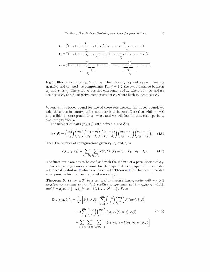
Next we consider the swap configuration among x1, x2 and xc. Let xj beat swap distance rj from xc, for j = 1, 2. We let δ1 be the number of positivecomponents of xc that are negative in both x1 and x2. Similarly, δ2 is thenumber of negative components of xc that are positive in both x1 and x2. SeeFigure 3. The swap distance between x1 and x2 is then r3 = r1 + r2 − δ1 − δ2.
Let r = (r1, r2), δ = (δ1, δ2) and r = min(r1, r2). We will study values ofr1, r2, r3, δ1, δ2 ranging over the following sets:
r1, r2 ∈ R = {1, . . . ,m}δ1 ∈ D1(r) = {max(0, r1 + r2 −m0), . . . , r}δ2 ∈ D2(r) = {max(0, r1 + r2 −m1), . . . , r}, and
r3 ∈ R3(r) = {max(1, r1 + r2 − 2r), . . . ,min(r1 + r2,m,m0 +m1 − r1 − r2)}.
He, Basu, Zhao & Owen/Stolarsky invariance for permutations 16
xc = (
m1︷ ︸︸ ︷+,+,+,+,+, · · · ,+,+,+,+,
m0︷ ︸︸ ︷−,−,−,−, · · · ,−,−,−,−,− )
x1 = (
m1︷ ︸︸ ︷+,+,+, · · · ,+,−,−,−, · · · ,−︸ ︷︷ ︸
r1
,
m0︷ ︸︸ ︷+,+,+, · · · ,+,+,+︸ ︷︷ ︸
r1
,−, · · · ,− )
x2 = (
m1︷ ︸︸ ︷+, · · · ,+,−,−, · · · ,−︸ ︷︷ ︸
δ1︸ ︷︷ ︸r2
,+, · · · ,+,
m0︷ ︸︸ ︷−, · · · ,−,+,+, · · ·︸ ︷︷ ︸
δ2
,+
︸ ︷︷ ︸r2
,−, · · · ,− )
Fig 3: Illustration of r1, r2, δ1 and δ2. The points xc, x1 and x2 each have m0
negative and m1 positive components. For j = 1, 2 the swap distance betweenxj and xc is rj . There are δ1 positive components of xc where both x1 and x2
are negative, and δ2 negative components of xc where both xj are positive.
Whenever the lower bound for one of these sets exceeds the upper bound, wetake the set to be empty, and a sum over it to be zero. Note that while r1 = 0is possible, it corresponds to x1 = xc and we will handle that case specially,excluding it from R.
The number of pairs (x`,xk) with a fixed r and δ is
c(r, δ) =
(m0
δ1
)(m1
δ2
)(m0 − δ1r1 − δ1
)(m1 − δ2r1 − δ2
)(m0 − r1r2 − δ1
)(m1 − r1r2 − δ2
). (4.8)
Then the number of configurations given r1, r2 and r3 is
c(r1, r2, r3) =∑δ1∈D1
∑δ2∈D2
c(r, δ)1(r3 = r1 + r2 − δ1 − δ2). (4.9)
The functions c are not to be confused with the index c of a permutation of x0.We can now get an expression for the expected mean squared error under
reference distribution 2 which combined with Theorem 4 for the mean providesan expression for the mean squared error of pc.
Theorem 5. Let x0 ∈ Sd be a centered and scaled binary vector with m0 > 1negative components and m1 > 1 positive components. Let ρ = yT
0x0 ∈ [−1, 1],and ρ = yT
0xc ∈ [−1, 1] for c ∈ {0, 1, . . . , N − 1}. Then
E2,c(p(y, ρ)2) =1
N2
[1(ρ > ρ) +
m∑r=1
(m0
r
)(m1
r
)P1(u(r), ρ, ρ)
+ 2
m∑r=1
(m0
r
)(m1
r
)P2(1, u(r), u(r), ρ, ρ)
+∑r1∈R
∑r2∈R
∑r3∈R3(r)
c(r1, r2, r3)P2(u1, u2, u3, ρ, ρ)
] (4.10)
He, Basu, Zhao & Owen/Stolarsky invariance for permutations 17
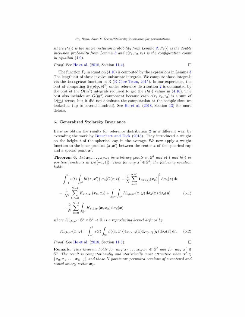
where P1(·) is the single inclusion probability from Lemma 2, P2(·) is the doubleinclusion probability from Lemma 3 and c(r1, r2, r3) is the configuration countin equation (4.9).
Proof. See He et al. (2018, Section 11.4).
The function P2 in equation (4.10) is computed by the expressions in Lemma 3.The lengthiest of these involve univariate integrals. We compute those integralsvia the integrate function in R (R Core Team, 2015). In our experience, thecost of computing E2(p(y, ρ)2) under reference distribution 2 is dominated bythe cost of the O(m3) integrals required to get the P2(·) values in (4.10). Thecost also includes an O(m4) component because each c(r1, r2, r3) is a sum ofO(m) terms, but it did not dominate the computation at the sample sizes welooked at (up to several hundred). See He et al. (2018, Section 13) for moredetails.
5. Generalized Stolarsky Invariance
Here we obtain the results for reference distribution 2 in a different way, byextending the work by Brauchart and Dick (2013). They introduced a weighton the height t of the spherical cap in the average. We now apply a weightfunction to the inner product 〈z,x′〉 between the center z of the spherical capand a special point x′.
Theorem 6. Let x0, . . . ,xN−1 be arbitrary points in Sd and v(·) and h(·) bepositive functions in L2([−1, 1]). Then for any x′ ∈ Sd, the following equationholds,∫ 1
−1v(t)
∫Sdh(〈z,x′〉)
∣∣∣∣σd(C(z; t))− 1
N
N−1∑k=0
1C(z;t)(xk)
∣∣∣∣2 dσd(z) dt
=1
N2
N−1∑k,`=0
Kv,h,x′(xk,x`) +
∫Sd
∫SdKv,h,x′(x,y) dσd(x) dσd(y)
− 2
N
N−1∑k=0
∫SdKv,h,x′(x,xk) dσd(x)
(5.1)
where Kv,h,x′ : Sd × Sd → R is a reproducing kernel defined by
Kv,h,x′(x,y) =
∫ 1
−1v(t)
∫Sdh(〈z,x′〉)1C(z;t)(x)1C(z;t)(y) dσd(z) dt. (5.2)
Proof. See He et al. (2018, Section 11.5).
Remark. This theorem holds for any x0, . . . ,xN−1 ∈ Sd and for any x′ ∈Sd. The result is computationally and statistically most attractive when x′ ∈{x0,x1, . . . ,xN−1} and those N points are permuted versions of a centered andscaled binary vector x0.

He, Basu, Zhao & Owen/Stolarsky invariance for permutations 18
We now show that the second moment in Theorem 5 holds as a special limitingcase of Theorem 6. In addition to vε from Section 3 we introduce η = (η1, η2) ∈(0, 1)2 and
hη(s) = η2 +1
η1(ωd−1
ωd(1− s2)d/2−1)
1(ρ 6 s 6 ρ+ η1). (5.3)
Using these results we can now establish the following theorem, which providesthe second moment of p(y, ρ) under reference distribution 2.
Theorem 7. Let x0 ∈ Sd be a centered and scaled binary vector with m0 > 1negative components and m1 > 1 positive components. Let x0,x1, . . . ,xN−1 bethe N =
(m0+m1
m0
)distinct permutations of x0. Let xc be one of the xk and
define pc by (4.1). Then
E2,c(p(y, ρ)2) =1
N2
N−1∑k,`=0
∫Sd−1
1(〈y,xk〉 > ρ)1(〈y,x`〉 > ρ) dσd−1(y∗)
where y = ρxc +√
1− ρ2y∗ and E2,c denotes expectation under reference dis-tribution 2(c).
Proof. The proof uses Theorem 6 with a sequence of h defined in (5.3) and vdefined in (3.3). See He et al. (2018, Section 11.6).
This result shows that we can use the invariance principle to derive the secondmoment of p(y, ρ) under reference distribution 2. The mean square in Theorem 7matches the second moment equation (3.6) in Proposition 1.
6. Two-sided p-values
In statistical applications it is more usual to report two-sided p-values. A con-servative approach is to use 2 min(p, 1 − p) where p is a one-sided p-value. Asharper choice is the two-sided p-value from (1.3) which we write here as
p(2) =1
N
N−1∑k=0
1(|xTky0| > |ρ|),
for ρ = xT0y0. For this section only, we use a superscript (2) to distinguish two-
sided p-values from their one-sided counterparts. We describe how to get two-
sided versions p(2)1 and p
(2)2 of our one-sided estimates as well as their respective
reference variances. If ρ = 0, then trivially p(2) = 1. From here on we assumethat ρ 6= 0.
We begin with p1. The two-sided version of p1(ρ) is p(2)1 = 2σd(C(y; |ρ|)). Also
E1(p(2)) = p(2)1 . We now consider the mean square for the two-sided estimate
He, Basu, Zhao & Owen/Stolarsky invariance for permutations 19
under reference distribution 1. For x1,x2 ∈ Sd with u = xT1x2, the two-sided
double inclusion probability under reference distribution 1 is
V2(u; t, d) =
∫Sd
1(|〈z,x1〉| > |t|)1(|〈z,x2〉| > |t|) dσd(z).
For t 6= 0, we write 1(|〈z,xj〉| > |t|) = 1(〈z,xj〉 > |t|) + 1(〈z, (−xj)〉 > |t|) forj = 1, 2 and expanding the product, we get
V2(u; t, d) = 2V2(u; |t|, d) + 2V2(−u; |t|, d).
By replacing V2(u; t, d) with V2(u; t, d) and p1(t) with 2σd(C(y; |t|)) in equa-
tion (3.8) of Theorem 3, we get a formula for Var1(p(2)1 ).
Next we obtain corresponding formulas under reference distribution 2. Forsome fixed c ∈ {0, 1, . . . , N − 1}, let uj = xT
j xc for j = 1, 2, and let u3 = xT1x2.
Let the decomposition of y with respect to xc be y = ρxc +√
1− ρ2y∗. Thetwo-sided inclusion probabilities are
P1(u1, ρ, ρ) =
∫Sd−1
1(|〈y,x1〉| > |ρ|
)dσd−1(y∗), and,
P2(u1, u2, u3, ρ, ρ) =
∫Sd−1
1(|〈y,x1〉| > |ρ|
)1(|〈y,x2〉| > |ρ|
)dσd−1(y∗),
where y∗ enters the integrands through y. After writing 1(|〈y,xj〉| > |ρ|) =1(〈y,xj〉 > |ρ|) + 1(〈y,−xj〉 > |ρ|) we find that
P1(u1, ρ, ρ) = P1(u1, ρ, |ρ|) + P1(−u1, ρ, |ρ|), and
P2(u1, u2, u3, ρ, ρ) = P2(u1, u2, u3, ρ, |ρ|) + P2(−u1, u2,−u3, ρ, |ρ|)+ P2(u1,−u2,−u3, ρ, |ρ|) + P2(−u1,−u2, u3, ρ, |ρ|).
In the expression for P2, notice that u3 changes to −u3 if and only if exactlyone of u1, u2 changes sign. This is because u3 = xT
1x2. Changing P1(u1, ρ, ρ)and P2(u1, u2, u3, ρ, ρ) to P1(u1, ρ, ρ) and P2(u1, u2, u3, ρ, ρ) respectively in The-
orems 4 and 5, yields expressions for E2,c(p(2)c ) and Var2,c(p
(2)c ).
7. Numerical Results
We consider two-sided p-values in this section. The main finding is that the rootmean squared error (RMSE) of p2 under reference distribution 2 is usually justa small multiple of p2 itself.
First we evaluate the accuracy of p1, the simple spherical cap volume ap-proximate p-value. We considered m0 = m1 in a range of values from 5 to 200.The values p1 ranged from just below 1 to 2 × 10⁻³⁰. We judge the accuracyof this estimate by RMSE1(p1) = (E1(p1(ρ) − p(y, ρ))2)1/2. As ρ → 1, p1 → 0and Figure 4a shows RMSE1 decreasing towards 0 in this limit. The RMSE also

He, Basu, Zhao & Owen/Stolarsky invariance for permutations 20
decreases with increasing sample size, as we would expect from the central limittheorem.
As seen in Figures 4a and 4b, the RMSE is not monotone in p1. Right atp1 = 1 we know that RMSE = 0 and around 0.1 there is a dip. The practicallyinteresting values of p1 are much smaller than 0.1, and the RMSE is monotonefor them.
A problem with p1 is that it can approach 0 even though p > 1/N must hold.The distribution 1 RMSE does not reflect this problem. By studying E2((p1(ρ)−p(y, ρ))2)1/2, we get a different result. In Figure 4c, the RMSE of p1 underdistribution 2 reaches a plateau as p1 goes to 0.
The estimator p2 = p0 performs better than p1 because it makes more useof the data, and it is never below 1/N . As seen in Figure 4d, the RMSE ofp2 very closely matches p2 itself as p2 decreases to zero. That is, the relativeerror |p2 − p|/p2 is well behaved for small p-values. In rare event estimation,that property is known as strong efficiency (Blanchet and Glynn, 2008) and canbe very hard to achieve. Here as p2 decreases to the granularity limit 1/N , itsRMSE actually decreases to 0. Eventually the distance from y0 to x0 is belowthe minimum interpoint distance among the xk and then, for a one-sided test,p2 = p = 1/N . The estimators p1 and p2, do not differ much for larger p-valuesas seen in Figure 5a. But in the limit as ρ → 1 we see that p1 → 0, while p2approaches the granularity limit 1/N instead.
Figure 5b compares the RMSE of the two estimators under distribution 2. Asexpected, p2 is more accurate. It also shows that the biggest differences occuronly when p1 goes below 1/N .
To examine the behavior of p2 more closely, we plot its coefficient of vari-ation in Figure 6. We see that the relative uncertainty in p2 is not extremelylarge. Even when the estimated p-values are as small as 10−30 the coefficient ofvariation is below 5.
Our derivations for p2 extend to pc for any c ∈ {0, 1, . . . , N−1}. The estimatorp2 = p0 never goes below 1/N because x0 ∈ C(y0, ρ). The same will hold forany c with 〈xc,y0〉 > 〈x0,y0〉. Among these, we took a particular interest in c =c∗ ≡ arg maxk〈xk,y0〉, the closest of all permutations of x0 to y0. This choicealso minimizes σd(Y2(c)) and serves to illustrate the generality of our theory. Forthe two-sided case c∗ = arg maxk |〈xk,y0〉|. We defined p3 = pc∗ = E(p(y, ρ))for y ∼ U(Y2(c∗)). Figure 2.7 in He (2016) compares p3 to p2 for the samesimulated cases reported here. There p3 tends to be larger (more conservative)than p2, though it does sometimes come out smaller. Figure 2.8 of He (2016)compares the RMSE of p3 to p2. The upward bias of p3 gave it a much largerRMSE.
Our simulations here all have m0 = m1. Section 12 of He et al. (2018) showssome simulations with m0 6= m1. The results are quite similar to the ones inthis section. The Parkinson’s data in Section 8 have m0 6= m1.

He, Basu, Zhao & Owen/Stolarsky invariance for permutations 21
●●●●
●●●●
●●●●
●●●●
●●●●
●●●●
●●●●
●●●●
●●●●
●●●●
●●●●
●●●●
●●●●
●●●●
●●●●
●●●●
●●●●
●●●●
●●●●
●●●●
●●●●
●●●●
●●●●
●●●●
●●●●
●●●●
●●●●
●●●●
●●●●
●●●●
●●●●
●●●●
●●●●
●●●●
●●●●
●●●●
●●●●
●●●●
●●●●
●●●●
●●●●
●●●●
●●●●
●●●●
●●●●●
●●●●
●●●●●●
●●●●●●
●●
●
●●●●
●●●●
●●●●
●●●●
●●●●
●●●●
●●●●
●●●●
●●●●
●●●●
●●●●
●●●●
●●●●
●●●●
●●●●
●●●●
●●●●
●●●●
●●●●
●●●●
●●●●
●●●●
●●●●
●●●●
●●●●
●●●●
●●●●
●●●●
●●●●
●●●●
●●●●
●●●●
●●●●
●●●●
●●●●
●●●●
●●●●
●●●●
●●●●
●●●●
●●●●
●●●●
●●●●
●●●●
●●●●
●●●●
●●●●●●●●●●
●●●●●
●
●●●●
●●●●
●●●●
●●●●
●●●●
●●●●
●●●●
●●●●
●●●●
●●●●
●●●●
●●●●
●●●●
●●●●
●●●●
●●●●
●●●●
●●●●
●●●●
●●●●
●●●●
●●●●
●●●●
●●●●
●●●●
●●●●
●●●●
●●●●
●●●●
●●●●
●●●●
●●●●
●●●●
●●●●
●●●●
●●●●
●●●●
●●●●
●●●●
●●●●
●●●●
●●●●
●●●●
●●●●
●●●●
●●●●
●●●●●●●●
●●
●●●●●
●
●●●●
●●●●
●●●●
●●●●
●●●●
●●●●
●●●●
●●●●
●●●●
●●●●
●●●●
●●●●
●●●●
●●●●
●●●●
●●●●
●●●●
●●●●
●●●●
●●●●
●●●●
●●●●
●●●●
●●●●
●●●●
●●●●
●●●●
●●●●
●●●●
●●●●
●●●●
●●●●
●●●●
●●●●
●●●●
●●●●
●●●●
●●●●
●●●●
●●●●
●●●●
●●●●
●●●●
●●●●
●●●●
●●●●
●●●●●●●●
●●
●●●●●
●●●●
●●●●
●●●●
●●●●
●●●●
●●●●
●●●●
●●●●
●●●●
●●●●
●●●●
●●●●
●●●●
●●●●
●●●●
●●●●
●●●●
●●●●
●●●●
●●●●
●●●●
●●●●
●●●●
●●●●
●●●●
●●●●
●●●●
●●●●
●●●●
●●●●
●●●●
●●●●
●●●●
●●●●
●●●●
●●●●
●●●●
●●●●
●●●●
●●●●
●●●●
●●●●
●●●●
●●●●
●●●●
●●●●
●●●●●●●
●
●
●
●●●
●●
●
●●●●
●●●●
●●●●
●●●●
●●●●
●●●●
●●●●
●●●●
●●●●
●●●●
●●●●
●●●●
●●●●
●●●●
●●●●
●●●●
●●●●
●●●●
●●●●
●●●●
●●●●
●●●●
●●●●
●●●●
●●●●
●●●●
●●●●
●●●●
●●●●
●●●●
●●●●
●●●●
●●●●
●●●●
●●●●
●●●●
●●●●
●●●●
●●●●
●●●●
●●●●
●●●●
●●●●
●●●●
●●●●
●●●●
●●●●●●●
●
●
●
●●●
●●
●
●●●●
●●●●
●●●●
●●●●
●●●●
●●●●
●●●●
●●●●
●●●●
●●●●
●●●●
●●●●
●●●●
●●●●
●●●●
●●●●
●●●●
●●●●
●●●●
●●●●
●●●●
●●●●
●●●●
●●●
●●●●●●●●●●●●●●●●●●●●●●●●●●●●●●●●●●●●●●
●●●
●●●●
●●●●
●●●●
●●●●
●●●●
●●●●
●●●●
●●●●
●●●●
●●●●
●●●●
●●●●
●●●●●●●
●
●
●
●●●
●●
●
●●●●●●●●●●●●●●●●●●●●●●●●●●●●●●●●●●●●●●●●●●●●●●●●●●●●●●●●●●●●●●●●●●●●●●●●●●●●●●●●●●●●●●●●●●●●●●●●●●●●●●●●●●●●●●●●●●●●●●●●●●●●●●●●●●●●●●●●
●●●●
●●●●
●●●●
●●●●
●●●●
●●●●
●●●●
●●●●
●●●●
●●●●
●●●●
●●●●
●●●●●●●
●
●
●
●●●
●●
●●●●●●●●●●●●●●●●●●●●●●●●●●●●●●●●●●●●●●●●●●●●●●●●●●●●●●●●●●●●●●●●●●●●●●●●●●●●●●●●●●●●●●●●●●●●●●●●●●●●●●●●●●●●●●●●●●●●●●●●●●●●●●●●●●●●●●●●
●●●●
●●●●
●●●●
●●●●
●●●●
●●●●
●●●●
●●●●
●●●●
●●●●
●●●●
●●●●
●●●●●●●●
●
●●●●
●●
●
−30
−20
−10
−30 −20 −10 0log10(phat1)
log1
0(R
MS
E1)
(m0, m1)●
●
●
●
●
●
●
●
●
5,510,1015,1520,2030,3040,4050,50100,100200,200
(a) RMSE1(p1).
●●●●●●●●●●●●●●●
●●●●●●●●●●●●●●●●●●●
●●●●●●●●●●●●●●●●●●●●●
●●●●●●●●●●●●●●●●●●
●●●●●●●●●●●●●●●●●●●●●●●●●●●●●●●●●●●●●●●●●●●●●●●●
●●●●●●●●●●●●
●●●●●●●●●●
●●●●●●●●●●●
●●●●●●●●●●●●●
●●●●●●●●●●●●●●●●●●●●●●●●●●●●
●●
●
●
●
●●●●●●●●●●●●●●●●●
●●●●●●●●●●●●●●●●●●●●●●●●●
●●●●●●●●●●●●●●●●●●●●●●●●●●●●●●●●●●●●●●●●●●●●●●●●●●●●●●●●●●●●●●●●●●●●●●●●●
●●●●
●●●●
●●●●
●●●●
●●●●
●●●●
●●●●●●
●●●●●●
●●●●●●●●●
●●●●●●●●●●●●●●●●●●●●●●●●●●●●●
●●●●●●
●
●
●
●
●
●●●●●●●●●●●●●●●●●●●
●●●●●●●●●●●●●●●●●●●●●●●●●●●●●●●●●●●●●●●●●●●●●●●●●●●●●●●●●●●●●●●●●●●●●●●●●●●●●●●●●●●●●●●
●●●●
●●●●●●
●●●●
●●●●
●●●●
●●●●
●●●●
●●●●●●
●●●●●●
●●●●●●●●●
●●●●●●●●●●●●●●●●●●●●●●●●●●●●●●●●
●●●●●●
●
●
●
●
●
●●●●●●●●●●●●●●●●●●●●●
●●●●●●●●●●●●●●●●●●●●●●●●●●●●●●●●●●●●●●●●●●●●●●●●●●●●●●●●●●●●●●●●●●●●●●●●●●●●●●●●●
●●●●●●●●●●●●●●●
●●●●
●●●●
●●●●
●●●●
●●●●●●
●●●●●●
●●●●●●●●
●●●●●●●●●●●●●●●●●●●●●●●●●●●●●●●●●●●●
●●●●●●
●
●
●
●
●●●●●●●●●●●●●●●●●●●●●●●●●
●●●●●●●●●●●●●●●●●●●●●●●●●●●●●●●●●●●●●●●●●●●●●●●●●●●●●●●●●●●●●●●●●●●●●●●●●●
●●●●●●●●●●●●●●●●
●●●●
●●●●
●●●●
●●●●
●●●●●●
●●●●●●
●●●●●●●●
●●●●●●●●●●●●●●●●●●●●●●●●●●●●●●●●●●●●●●
●●●●●●
●
●
●
●
●
●●●●●●●●●●●●●●●●●●●●●●●●●●●●●●●
●●●●●●●●●●●●●●●●●●●●●●●●●●●●●●●●●●●●●●●●●●●●●●●●●●●●●●●●●●●●●●●●●●
●●
●
●●●●●●●●●●●●●●
●●●●
●●●●
●●●●
●●●●
●●●●●●
●●●●●●
●●●●●●●●
●●●●●●●●●●●●●●
●●●●●●●●●●●●●●●●●●●●●●●●●●●●●●●
●
●
●
●
●
●●●●●●●●●●●●●●●●●●●●●●●●●●●●●●●●●●●●●●●●●●●●●●●●●●●●●●●●●●●●●●●●●●●●●●●●●●●●●●●●●●●●
●●●●●●●●
●
●●●
●
●
●
●
●●●●●●●●●●●●●●
●●●●
●●●●
●●●●
●●●●
●●●●●●
●●●●●●
●●●●●●●●
●●●●●●●●●●●●●●●●●●●●●●●●●●●●●●●●●●●●●●●
●●●●●●
●
●
●
●
●
●●●●●●●●●●●●●●●●●●●●●●●●●●●●●●●●●●●●●●●●●●●●●●●●●●●●●●●●●●●●●●●●●●●●●●●●●●●●●●●●●●
●●●●●●●
●
●
●
●
●
●
●
●
●
●
●●●●●●●●●●●●●
●●●●
●●●●
●●●●
●●●●
●●●●●●
●●●●●●
●●●●●●●●
●●●●●●●●●●●●
●●●●●●●●●●●●●●●●●●●●●●●●●●●●●●●●●●●
●
●
●
●
●●●●●●●●●●●●●●●●●●●●●●●●●●●●●●●●●●●●●●●●●●●●●●●●●●●●●●●●●●●●●●●●●●●●●●●●●●●●●●●
●●●●●●●
●●
●
●
●
●
●
●
●
●
●
●
●
●●●●●●●●●●●●
●●●●
●●●●
●●●●
●●●●
●●●●●
●●●●●●
●●●●●●●
●●●●●●●●●
●●●●●●●●●●●●●●●●●●●●●●●●●●●●●●●●●●●
●●●●●●
●
●
●
●
●
−8
−6
−4
−2
−2.0 −1.5 −1.0 −0.5 0.0log10(phat1)
log1
0(R
MS
E1)
(m0, m1)●
●
●
●
●
●
●
●
●
5,510,1015,1520,2030,3040,4050,50100,100200,200
(b) RMSE1(p1) zoomed.
●●●●●●●●●●●●●●●●●●●●●●●●●●●●●●
●●●●●●●●●●●●●●●●●●●●●●●●●●●●●
●●●●●●●●●●●●●●●●●●●●●●●●●●●●
●
●●●●●●●●●●●●●●●●●●●●●●●●●●●●●
●●●●●●●●●●●●
●●●●●●●●●●●●●●●●●
●
●●●●●●●●●●●●
●●
●●
●●
●●
●
●
●
●
●
●
●●
●
●●●●●●●●●●●
●●
●●
●●
●
●
●
●
●
●
●
●
●
●
●
●
● ● ● ● ● ● ● ●●
●●
●●
●
●
●
●
●
●
●
●
●
●
●
●
●
●
●
●
● ● ● ● ● ● ●●
●●
●
●
●
●
●
●
●
●
●
●
●
●
●
●
●
●
●
●
●
−60
−40
−20
0
−120 −90 −60 −30 0log10(phat1)
log1
0(R
MS
E1U
ND
ER
2)
(m0, m1)●
●
●
●
●
●
●
●
●
5,510,1015,1520,2030,3040,4050,5070,70100,100
(c) RMSE2(p1).
●●●●●●●●●
●
●●●●●●●●●●●●●●●●
●●●
●
●●●
●
●●●●●●●●●●●●●●●●●
●●●●●●●
●
●
●●●●●●●●●●●●●●●●●●
●●●●
●●●●●
●
●●●●●●●●●●●●●●●●
●●●●●●●●●●●●●
●●●●●●●●●●●●●
●●●●●
●●
●●
●●
●●
●●●
●
●●●●●●●●●●●●●●●
●●
●●
●●
●
●
●
●
●
●●
●
●●●●●●●●●●●●●
●●
●●
●
●
●
●
●
●
●
●
●
●
●●
●●●●●●●●●●●
●●
●
●
●
●
●
●
●
●
●
●
●
●
●
●
●
●
●●●●●●●●●●
●
●
●
●
●
●
●
●
●
●
●
●
●
●
●
●
●
●
●
−60
−40
−20
0
−60 −40 −20 0log10(phat2)
log1
0(R
MS
E2)
(m0, m1)●
●
●
●
●
●
●
●
●
5,510,1015,1520,2030,3040,4050,5070,70100,100
(d) RMSE2(p2).
Fig 4: RMSEs for p1 and p2 under reference distributions 1 and 2. The x-axisshows the estimate p1 or p2 as ρ varies from 1 to 0. Here m0 = m1.
8. Comparison to saddlepoint approximation
The small relative error property of p2 is similar to the relative error propertyin saddlepoint approximations, and so we compare our methods to saddlepointsapproximations. Reid (1988) surveys saddlepoint approximations and Robinson(1982) develops them for permutation tests of linear statistics. When the truep-value is p, the saddlepoint approximation ps satisfies ps = p(1 + O(1/n)).Because we do not know the implied constant in O(1/n) or the n at whichit takes effect, the saddlepoint approximation does not provide a computableupper bound for the true permutation p-value p.
Figure 7 compares our estimates to each other and to the saddlepoint ap-

He, Basu, Zhao & Owen/Stolarsky invariance for permutations 22
●●●●●●●●●●●●●●●●●●●●●●●●●●●●●●
●●●●●●●●●●●●●●●●●●●●●●●●●●●●●
●●●●●●●●●●●●●●●●●●●●●●●●●●●●●
●●●●●●●●●●●●●●●●●●●●●●●●●●●●●
●●●●●●●●●●●●●
●●●●●●●●●●●●●●●●●
●●●●●●●●●●●●●
●●
●●
●●
●
●
●
●
●
●
●
●
●
●
●●●●●●●●●●●●
●●
●●
●
●
●
●
●
●
●
●
●
●
●
●
●
● ● ● ● ● ● ● ● ● ●●
●●
●
●
●
●
●
●
●
●
●
●
●
●
●
●
●
●
● ● ● ● ● ● ● ●●
●●
●
●
●
●
●
●
●
●
●
●
●
●
●
●
●
●
●
●
−60
−40
−20
0
−120 −90 −60 −30 0log10(phat1)
log1
0(ph
at2)
(m0, m1)●
●
●
●
●
●
●
●
●
5,510,1015,1520,2030,3040,4050,5070,70100,100
(a)
●●●●●●●●●●
●
●
●
●
●
●
●
●
●
●
●
●
●●●●●●●
●●●●●●●●
●
●
●
●
●
●
●
●
●
●
●
●
●
●
●
●●●●●●●
●●●●●
●
●
●
●
●
●
●
●
●
●
●●●
●
●
●
●
●
●●●●●●
●●●●●
●
●
●
●
●
●
●
●
●●●●●●
●
●
●
●
●
●●●●●
●●●●
●
●
●
●
●
●
●
●
●●●
●●●●●●
●
●
●
●
●●●●●
●●●
●
●
●
●
●
●
●
●
●●●●
●●●
●
●●●
●
●
●
●
●●●
●●●
●
●
●
●
●
●
●
●●●●●●
●●
●
●
●
●●
●
●
●
●●●
●●
●
●
●
●
●
●
●
●● ● ● ● ● ● ●
●●
●
●
●
● ●
●
●
●
● ●
●●
●
●
●
●
●
●● ● ● ● ● ● ● ● ● ● ●
●
●
●
●
● ●
●
●
● ●
0.00
0.25
0.50
0.75
1.00
−120 −90 −60 −30 0log10(phat1)
RM
SE
2/R
MS
E1U
ND
ER
2
(m0, m1)●
●
●
●
●
●
●
●
●
5,510,1015,1520,2030,3040,4050,5070,70100,100
(b)
Fig 5: Comparison of p1 and p2. Panel (a) plots log10(p2) againstlog10(p1) for varying ρ with a 45 degree reference line. Panel (b) plotsRMSE2(p2)/RMSE2(p1) versus log10(p1) for varying ρ.
●●●●●●●●●●●●●●●●●●●●●●●●●●●●●●●●●●●●●●
●●●●●●●●●●●●●●●●●●●●●●●●●●●●
●●●●●●●●●●●●●●●●●●●●●●●●●●●●
●●●●●●●●●●●●●●●●●●●●●●●●●●●●
●●●●●
●
●●●●●
●●
●●
●●
●●
●●●●●●●●●●●●●●
●
●
●
●●●●
●●
●●
●●
●●
●●
● ● ● ●●●●●●●●
●
●
●
●
●●●
●●
●
●
●
●
●●
●●
●●
● ● ●●●●●●●
●
●
●
●
●
●●●
●
●
●
●
●
●
●
●
●
●●
●●
● ●●●●●●
●
●
●
●
●
●
●
●●
●
●
●
●
●
●
●
●
●
●
●●
●● ●0
5
10
−60 −40 −20 0log10(phat2)
RM
SE
2/ph
at2
(m0, m1)●
●
●
●
●
●
●
●
●
5,510,1015,1520,2030,3040,4050,5070,70100,100
Fig 6: Coefficient of variation RMSE2(p2)/p2 versus log10(p2) for varying ρ.
proximation, equation (1) from Robinson (1982). It includes the estimator p3mentioned at the end of Section 7. The simulated data have the Exp(1) dis-tribution under the control condition and are 2 + Exp(1) under the affectedcondition. The sample sizes were m0 = m1 = 10 making it feasible to computethe exact permutation p-value. We ran 500 independent simulations, comparingtwo-sided p-values. Chapter 2 of He (2016) considers simulations from some ad-ditional distributions. Those had t(5), N (0, 1) and U(0, 1) for the control data

He, Basu, Zhao & Owen/Stolarsky invariance for permutations 23
phat3 saddle.point
phat1 phat2
0.1 10.0 0.1 10.0
0
25
50
75
0
25
50
75
phat/p.exact
coun
t
Fig 7: Simulation results p/p as described in the text, for Y0,iiid∼ Exp(1), and
Y1,iiid∼ Exp(1) + 2.
while the affected condition data are shifted versions of these distributions.In these simulations, the naive spherical cap estimator p1, with no good
relative error properties, is consistently least accurate and is often much smallerthan the true p. The saddlepoint estimate is very accurate but tends to comeout slightly smaller than the true p. The estimators p2 and p3 are less likely tobe below p than the saddlepoint estimate, and by construction, they are neverbelow the granularity limit. Qualitatively similar results happened for the otherdistributions. See He (2016, Chapter 2). The accuracy of all of these p-valueestimates tends to be better for lighter tailed Yi.
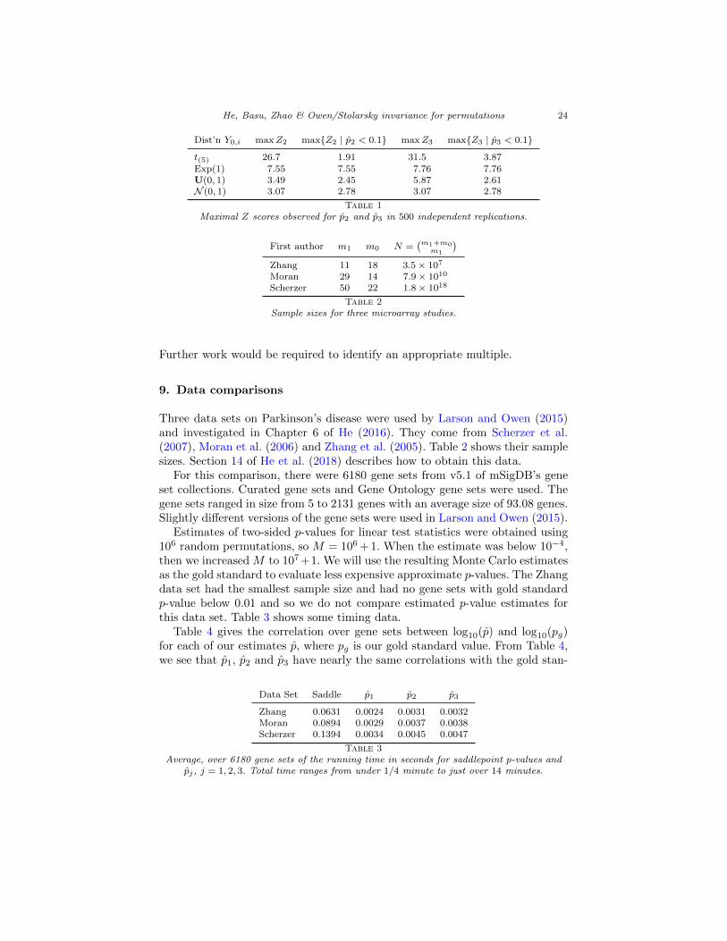
We can also construct Z scores, Z2 = (p − p2)/RMSE2 and a similar Z3. Ifthese take large values, then it means that p is too small and, moreover, thatour computed RMSE does not diagnose it. The largest Z scores we observed arein Table 1. The largest Z values arose for exponential data with p
.= 0.89 and
p2.= 0.78
.= p3. Such large p-values are not very important and so maximal Z
scores are also shown among estimated p-values below 0.1.The Z values are not very extreme. This suggests that it might be feasible to
get a conservative p-value estimate by adding some multiple of RMSE2 to p2.
He, Basu, Zhao & Owen/Stolarsky invariance for permutations 24
Dist’n Y0,i maxZ2 max{Z2 | p2 < 0.1} maxZ3 max{Z3 | p3 < 0.1}
t(5) 26.7 1.91 31.5 3.87Exp(1) 7.55 7.55 7.76 7.76U(0, 1) 3.49 2.45 5.87 2.61N (0, 1) 3.07 2.78 3.07 2.78
Table 1Maximal Z scores observed for p2 and p3 in 500 independent replications.
First author m1 m0 N =(m1+m0
m1
)Zhang 11 18 3.5× 10⁷
Moran 29 14 7.9× 10¹⁰
Scherzer 50 22 1.8× 10¹⁸
Table 2Sample sizes for three microarray studies.
Further work would be required to identify an appropriate multiple.
9. Data comparisons
Three data sets on Parkinson’s disease were used by Larson and Owen (2015)and investigated in Chapter 6 of He (2016). They come from Scherzer et al.(2007), Moran et al. (2006) and Zhang et al. (2005). Table 2 shows their samplesizes. Section 14 of He et al. (2018) describes how to obtain this data.
For this comparison, there were 6180 gene sets from v5.1 of mSigDB’s geneset collections. Curated gene sets and Gene Ontology gene sets were used. Thegene sets ranged in size from 5 to 2131 genes with an average size of 93.08 genes.Slightly different versions of the gene sets were used in Larson and Owen (2015).
Estimates of two-sided p-values for linear test statistics were obtained using106 random permutations, so M = 106 + 1. When the estimate was below 10−4,then we increased M to 107+1. We will use the resulting Monte Carlo estimatesas the gold standard to evaluate less expensive approximate p-values. The Zhangdata set had the smallest sample size and had no gene sets with gold standardp-value below 0.01 and so we do not compare estimated p-value estimates forthis data set. Table 3 shows some timing data.
Table 4 gives the correlation over gene sets between log10(p) and log10(pg)for each of our estimates p, where pg is our gold standard value. From Table 4,we see that p1, p2 and p3 have nearly the same correlations with the gold stan-
Data Set Saddle p1 p2 p3
Zhang 0.0631 0.0024 0.0031 0.0032Moran 0.0894 0.0029 0.0037 0.0038Scherzer 0.1394 0.0034 0.0045 0.0047
Table 3Average, over 6180 gene sets of the running time in seconds for saddlepoint p-values and
pj , j = 1, 2, 3. Total time ranges from under 1/4 minute to just over 14 minutes.

He, Basu, Zhao & Owen/Stolarsky invariance for permutations 25
Data source Corr. # sets p1 p2 p3 psaddle
Moran small Pearson 3594 0.9997 0.9997 0.9997 0.9934Moran small Kendall 3594 0.9857 0.9857 0.9866 0.9397Moran tiny Pearson 253 0.9684 0.9688 0.9787 0.7930Moran tiny Kendall 253 0.8820 0.8820 0.9033 0.6863
Scherzer small Pearson 504 0.9997 0.9997 0.9997 0.9836Scherzer small Kendall 504 0.9871 0.9871 0.9871 0.8965Scherzer tiny Pearson 16 0.9950 0.9950 0.9956 0.8794Scherzer tiny Kendall 16 0.9500 0.9500 0.9500 0.7833
Table 4Pearson and Kendall correlations over gene sets, between four approximations log10(p) andlog10(pg), where pg is an expensive gold standard estimate. Here ‘small’ refers to only the3594 gene sets with pg < 0.05 for Moran (504 for Scherzer), while ‘tiny’ refers to 253 gene
sets with pg < 10−4 (Moran) or 16 gene sets with pg < 10−3 (Scherzer).
dard; indeed they correlate highly with each other. They correlate with thegold standard estimate much more closely than the saddlepoint estimator does.The estimate p3 is frequently most correlated with the gold standard. Thesecorrelations capture the ability of a method to correctly rank the gene sets bysignificance. Figures in Chapter 6 of He (2016) give scatterplots that show theaccuracy of each p for pg. These show the saddlepoint estimator is biased slightlylow and p3 is biased slightly high.
10. Discussion
We have constructed approximations to the permutation p-value using proba-bility and spherical geometry. Many other approximation methods have beenproposed for permutation tests. For instance, Zhou et al. (2009) fit approxi-mations by moments in the Pearson family. Larson and Owen (2015) fit Gaus-sian and beta approximations to linear statistics and gamma approximationsto quadratic statistics for gene set testing problems. Knijnenburg et al. (2009)fit generalized extreme value distributions to the tails of sampled permutationvalues.
Our proposed estimator p2 has a small relative error, as measured by RMSEin the limit as ρ → 1. The well-known saddlepoint estimator also has a smallrelative error of O(1/n) extending to very small p-values. We found it performedwell on our simulated data but not as well on the Parkinson’s disease gene sets.
None of these approximations come with an all inclusive p-value that accountsfor both numerical uncertainty of the estimation and sampling uncertainty be-hind the original data. Monte Carlo sampling of permutations has such a p-value,but it is computationally infeasible to attain very small p-values that way, andso a gap remains.
We have employed reference distributions in an effort to address this gap. Weselect a set Y containing y0 and find the first two moments of p(y, ρ) for y ∼U(Y). If the data y0 were actually sampled from our reference distribution, thenwe could get an all inclusive conservative p-value via the Chebychev inequality.
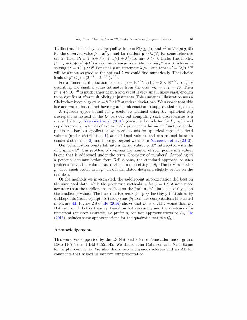
He, Basu, Zhao & Owen/Stolarsky invariance for permutations 26
To illustrate the Chebychev inequality, let µ = E(p(y, ρ)) and σ2 = Var(p(y, ρ))for the observed value ρ = xT
0y0 and for random y ∼ U(Y) for some referenceset Y. Then Pr(p > µ + λσ) 6 1/(1 + λ2) for any λ > 0. Under this model,p∗ = µ+λσ+1/(1+λ2) is a conservative p-value. Minimizing p∗ over λ reduces tosolving 2λ = σ(1+λ2)2. For small p we anticipate λ� 1 and hence λ′ = (2/σ)1/3
will be almost as good as the optimal λ we could find numerically. That choiceleads to p∗ 6 µ+ (21/3 + 2−2/3)σ2/3.
For a numerical illustration, consider µ = 10−30 and σ = 3× 10⁻³⁰, roughlydescribing the small p-value estimates from the case m0 = m1 = 70. Thenp∗ 6 4×10⁻²⁰ is much larger than µ and yet still very small, likely small enoughto be significant after multiplicity adjustments. This numerical illustration uses aChebychev inequality at λ′
.= 8.7×10⁹ standard deviations. We suspect that this
is conservative but do not have rigorous information to support that suspicion.A rigorous upper bound for p could be attained using L∞ spherical cap
discrepancies instead of the L2 version, but computing such discrepancies is amajor challenge. Narcowich et al. (2010) give upper bounds for the L∞ sphericalcap discrepancy, in terms of averages of a great many harmonic functions at thepoints xi. For our application we need bounds for spherical caps of a fixedvolume (under distribution 1) and of fixed volume and constrained location(under distribution 2) and those go beyond what is in Narcowich et al. (2010).
Our permutation points fall into a lattice subset of Rd intersected with theunit sphere Sd. Our problem of counting the number of such points in a subsetis one that is addressed under the term ‘Geometry of numbers’. According toa personal communication from Neil Sloane, the standard approach to suchproblems is via the volume ratio, which in our setting is p1. The new estimatorp2 does much better than p1 on our simulated data and slightly better on thereal data.
Of the methods we investigated, the saddlepoint approximation did best onthe simulated data, while the geometric methods pj for j = 1, 2, 3 were moreaccurate than the saddlepoint method on the Parkinson’s data, especially so onthe smallest p-values. The best relative error |p− p|/p for tiny p is attained bysaddlepoints (from asymptotic theory) and p2 from the computations illustratedin Figure 4d. Figure 2.8 of He (2016) shows that p3 is slightly worse than p2.Both are much better than p1. Based on both accuracy and the existence of anumerical accuracy estimate, we prefer p2 for fast approximations to LG. He(2016) includes some approximations for the quadratic statistic QG.
Acknowledgements
This work was supported by the US National Science Foundation under grantsDMS-1407397 and DMS-1521145. We thank John Robinson and Neil Sloanefor helpful comments. We also thank two anonymous referees and an AE forcomments that helped us improve our presentation.

He, Basu, Zhao & Owen/Stolarsky invariance for permutations 27
References
Ackermann, M. and Strimmer, K. (2009). A general modular framework forgene set enrichment analysis. BMC Bioinformatics, 10:1–20.
Barnard, G. A. (1963). Discussion of the spectral analysis of point processes(by M. S. Bartlett). Journal of the Royal Statistical Society, Series B, 25:294.
Bilyk, D., Dai, F., and Matzke, R. (2016). Stolarsky principle and energy opti-mization on the sphere. Technical report, arXiv:1611.04420.
Blanchet, J. and Glynn, P. (2008). Efficient rare-event simulation for the maxi-mum of heavy-tailed random walks. The Annals of Applied Probability, pages1351–1378.
Brauchart, J. and Dick, J. (2013). A simple proof of Stolarsky’s invarianceprinciple. Proceedings of the American Mathematical Society, 141(6):2085–2096.
Fadista, J., Manning, A. K., Florez, J. C., and Groop, L. (2016). The (in) famousGWAS p-value threshold revisited and updated for low-frequency variants.European Journal of Human Genetics, 24(8):1202–1205.
He, H. Y. (2016). Efficient Permutation-Based P-Value Estimation for GeneSet Tests. PhD thesis, Stanford University.
He, H. Y., Basu, K., Zhao, Q., and Owen, A. B. (2018). Supplement to: Permu-tation p-value approximation via generalized Stolarsky invariance. Technicalreport, Stanford University.
Jiang, Z. and Gentleman, R. (2007). Extensions to gene set enrichment. Bioin-formatics, 23(3):306–313.
Knijnenburg, T. A., Wessels, L. F. A., Reinders, M. J. T., and Shmulevich,I. (2009). Fewer permutations, more accurate p-values. Bioinformatics,25(12):i161–i168.
Larson, J. L. and Owen, A. B. (2015). Moment based gene set tests. BMCBioinformatics, 16(1):132.
Lee, Y. and Kim, W. C. (2014). Concise formulas for the surface area of theintersection of two hyperspherical caps. Technical report, Korea AdvancedInstitute of Science and Technology.
Lehmann, E. L. and Romano, J. P. (2005). Testing Statistical Hypotheses.Springer, New York, 3rd edition.
Mardia, K. V. and Jupp, P. E. (2000). Directional Statistics. John Wiley &Sons Ltd., Chichester, UK.
Moran, L. B., Duke, D. C., Deprez, M., Dexter, D. T., Pearce, R. K. B., andGraeber, M. B. (2006). Whole genome expression profiling of the medial andlateral substantia nigra in Parkinson’s disease. Neurogenetics, 7(1):1–11.
Narcowich, F. J., Sun, X., Ward, J. D., and Wu, Z. (2010). Leveque typeinequalities and discrepancy estimates for minimal energy configurations onspheres. Journal of Approximation Theory, 162(6):1256–1278.
Niederreiter, H. (1992). Random Number Generation and Quasi-Monte CarloMethods. SIAM, Philadelphia, PA.
R Core Team (2015). R: A Language and Environment for Statistical Comput-ing. R Foundation for Statistical Computing, Vienna, Austria.
He, Basu, Zhao & Owen/Stolarsky invariance for permutations 28
Reid, N. (1988). Saddlepoint methods and statistical inference. Statistical Sci-ence, pages 213–227.
Robinson, J. (1982). Saddlepoint approximations for permutation tests andconfidence intervals. Journal of the Royal Statistical Society, Series B, pages91–101.
Scherzer, C. R., Eklund, A. C., Morse, L. J., Liao, Z., Locascio, J. J., Fefer,D., Schwarzschild, M. A., Schlossmacher, M. G., Hauser, M. A., Vance, J. M.,Sudarsky, L. R., Standaert, D. G., Growdon, J. H., Jensen, R. V., and Gullans,S. R. (2007). Molecular markers of early Parkinson’s disease based on geneexpression in blood. Proc Natl Acad Sci, 104(3):955–60.
Stolarsky, K. B. (1973). Sums of distances between points on a sphere. II.Proceedings of the American Mathematical Society, 41(2):575–582.
Tian, L., Greenberg, S. A., Kong, S. W., Altschuler, J., Kohane, I. S., andPark, P. J. (2005). Discovering statistically significant pathways in expressionprofiling studies. PNAS, 102(38):13544–13549.
Zhang, Y., James, M., Middleton, F. A., and Davis, R. L. (2005). Transcrip-tional analysis of multiple brain regions in Parkinson’s disease supports theinvolvement of specific protein processing, energy metabolism, and signalingpathways, and suggests novel disease mechanisms. American J Med Genet BNeuropsychiatry Genet, 137B(1):5–16.
Zhou, C., Wang, H. J., and Wang, Y. M. (2009). Efficient moments-basedpermutation tests. In Advances in Neural Information Processing Systems,pages 2277–2285.