SCA2010-A073 1/12

PERMEABILITY MEASUREMENT ON SMALL ROCK SAMPLES

R. Lenormand(1), F. Bauget(1), Gabriel Ringot(2)

(1)Cydarex, (2)ECEM

This paper was prepared for presentation at the International Symposium of the Society of Core Analysts held in Halifax, Nova Scotia, Canada, 4-7 October, 2010

ABSTRACT The paper describes several methods for measuring permeabilities on small rock samples with size from 0.5 to 2 cm. In the first method, a small rock sample (below 1 cm3) is first embedded in a resin and a 2 to 5 mm thick disc is cut, polished and placed in a core holder under a press. The permeability is then derived from a gas flowing through the rock. This method can be used in a very large range of permeabilities, from nanoD to several Darcy. The second method is based on a pulse decay of a viscous liquid (Darcylog method) or a gas surrounding a small chunk of rock placed in a container under pressure (volume around 1 cm3). For both gas and liquid, the pressure is quickly decreased by releasing a spring attached to a piston. For all the methods, numerical calculations were developed taking account of the Klinkenberg effect, with automatic history matching. The main result is the possibility to measure gas permeabilities from less than 1 nanoD to several Darcy. In the range of the nanoD, both simulations and experiments show that the stabilization time needs near 1 hour, even for sample thickness of a few mm. The domains of utilization of the various methods are finally displayed on a schematic diagram. INTRODUCTION There is an increasing demand for petrophysical measurements on samples of size around or below the centimeter. In most of cases, these small samples are used when regular cylindrical plugs are not available: fractured or highly laminated cores, side wall cores or drill cuttings [1]. Recently, some companies are also able to recover “micro-cores” of centimeter size during drilling [2], [3]. These small samples have the advantage of faster cleaning (molecular diffusion or multiphase displacements scale as the square of the size) and also faster measurements for low permeability. The main drawback is the lack of representativity for the "large scale" permeability. The measurements give a "matrix" permeability, vugs and fractures being less represented. However, this is useful information since the oil is trapped in this matrix. Using our expertise on drill cuttings [4], [5] we have tested several techniques to measure permeabilities on small rock samples: - Miniplugs: when small cylinders are available, generally used for microscanner [6].

SCA2010-A073 2/12

- Resin Discs: the piece of rock is embedded in resin and a slice of several mm is cut, following a technique already used for cuttings [7].

- Open Surface: without embedding, the entire rock surface is exposed to a pulse of pressure in a cell. Depending on the range of permeability, either a liquid or a gas is used:

o for "reservoir" permeabilities, a viscous liquid is used in the Darcylog method developed by IFP for cuttings,

o for low permeabilities, a gas pressure pulse is used, like in the original method developed by Luffel [8], [9] using a piston following a method published by IFP [10].

In a first part we will recall the main problems that are linked to these measurements. PHYSICAL BACKGROUND For measurements, we use both steady-state and unsteady-state methods (see API [11] or Jannot et al. [12]). The samples used in this study have a very large range of permeabilities leading to high and very low flow rates. Non-Darcy flows are involved, as well as thermal effects that are often underestimated in this kind of experiments (and misinterpreted as inertial or Klinkenberg effects):

Inertial effects They appear for high flow rates of gas, when the Reynolds number (Re) becomes of the order of unity [13], [14]. In the interpretation, we always calculate the Re to decide if this effect must be taken into account.

Klinkenberg effect With gas flowing through a porous medium, two extreme cases can be distinguished:

1. Poiseuille's flow: the collisions between molecules lead to the notion of viscosity and the Darcy’s approach is valid.

2. Knudsen's flow [15]: the characteristic pore size is negligible in comparison with the mean free path of the molecules. There are no collisions between molecules but only between solid walls and molecules.

The Klinkenberg effect corresponds to an intermediate case where the fluid is assumed continuous with a given viscosity and slip conditions are added to take account of the collision with the solid wall. Experimentally, this leads to a relation between the permeability at high pressure Kl (also called "liquid" permeability), the gas permeability Kg and the absolute pressure P:

1g lbK KP

⎛ ⎞= +⎜ ⎟⎝ ⎠

(1)

Important remark: This local relation, valid on any section along the sample, shows that the gas permeability depends on the position through the pressure. It can be integrated along the sample for a permanent flow, taking into account the compressibility of a gas following Boyle's law. It can be easily shown that for a linear, isothermal and permanent flow, the macroscopic flow can be described by an "average" gas permeability <Kg> assumed uniform such as:

SCA2010-A073 3/12

0

10

20

30

40

50

0 0.2 0.4 0.6 0.8 11/<P> (1/bar)

Kg

(nan

oD) Pulse-decay

Steady-state

KL = 1.5 nDb = 32 bar

0

10

20

30

40

50

0 0.2 0.4 0.6 0.8 11/<P> (1/bar)

Kg

(nan

oD) Pulse-decay

Steady-state

KL = 1.5 nDb = 32 bar

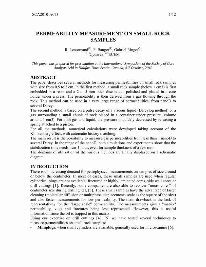
Figure 1 – Numerical calculation of gas permeability Kg as function of average pressure for a pulse-decay experiment. The straight line is the standard Klinkenberg correlation used in the simulation

1g lbK KP

⎛< >= +⎜⎞⎟< >⎝ ⎠

(2)

where <P>=(Pin+Pout)/2. That justifies the standard method for the determination of b and Kl: the experiment is interpreted as a gas flow with a uniform permeability <Kg> which is plotted as fraction of 1/<P>. However, the analytical integration is no longer possible for a pulse decay experiment then, if interpreted with a uniform <Kg>, there is no longer a linear relationship with the average pressure. Figure 1 shows the result of a numerical simulation for a pulse-decay experiment interpreted with average parameters (eq. 2). That may explain why transient experiments seem to overestimate the permeabilities as observed by Carles [10] and also Rushing [16].

Adiabatic expansion or compression Gas temperature decreases (or increases) when the gas is quickly expanded (or compressed) in an empty volume such as the dead volume at the entrance of the core during a pulse decay experiment. The variation of temperature is function of the ratio of pressures and is around 60°C for a pressure (absolute) ratio of two.

Joule-Thomson expansion Joule–Thompson is a thermal effect related to the slow expansion of a gas through a porous medium and can be positive or negative depending on the nature of the gas (see the recent SCA paper by Maloney and Briceno [17]). The cooling is proportional to the difference of pressure, with a coefficient equal to 0.23 °K/bar for air. This cooling is compensated by heat transfer with the surrounding set up and the resulting temperature depends on the flow rate. For a mixture of around 50% of N2 and He the coefficients of opposite signs compensate and the mixture present no Joule-Thompson effect [18]. NUMERICAL SIMULATIONS The interpretations were performed using the commercial software CYDAR. For the "resin discs" experiments the model is in one dimension. For the "open surface", several geometries are used, cylindrical, spherical, flat discs, infinite cylinders, etc. Klinkenberg and Forchheimer corrections can be used. The numerical scheme is implicit and the system is solved using a Newton-Raphson algorithm. The initial pressure condition can be non-uniform, in order to describe a transient flow starting after a steady-state. Parameters such as permeability, Klinkenberg coefficient or inertial parameters can be optimized using a nonlinear least-squares minimization algorithm. The cost function is calculated on inlet, outlet, or deference of pressures, depending on the measured parameter.

SCA2010-A073 4/12

MINIPLUGS

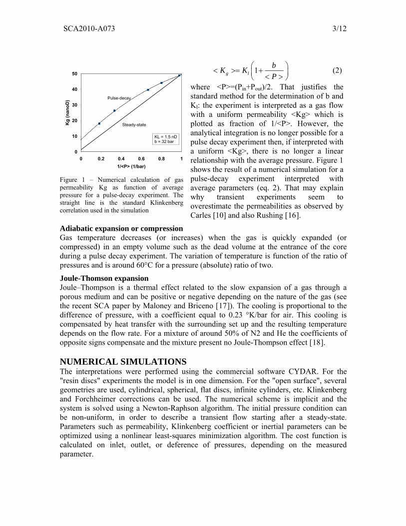
Figure 2 - example of miniplug with the

silicone tube

P1 - Fontainebleau Sandstone

time s

3.02.52.01.51.00.50.0

Pres

sure

mba

r

100

80

60

40

20

0

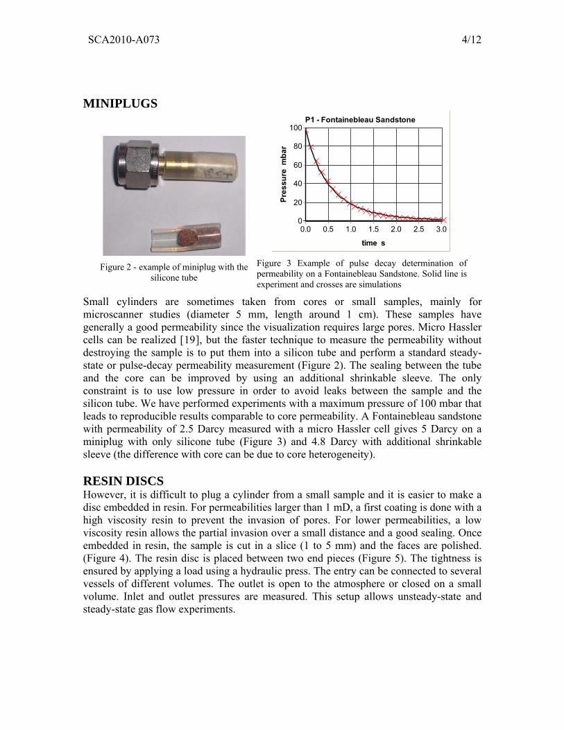
Figure 3 Example of pulse decay determination of permeability on a Fontainebleau Sandstone. Solid line is experiment and crosses are simulations

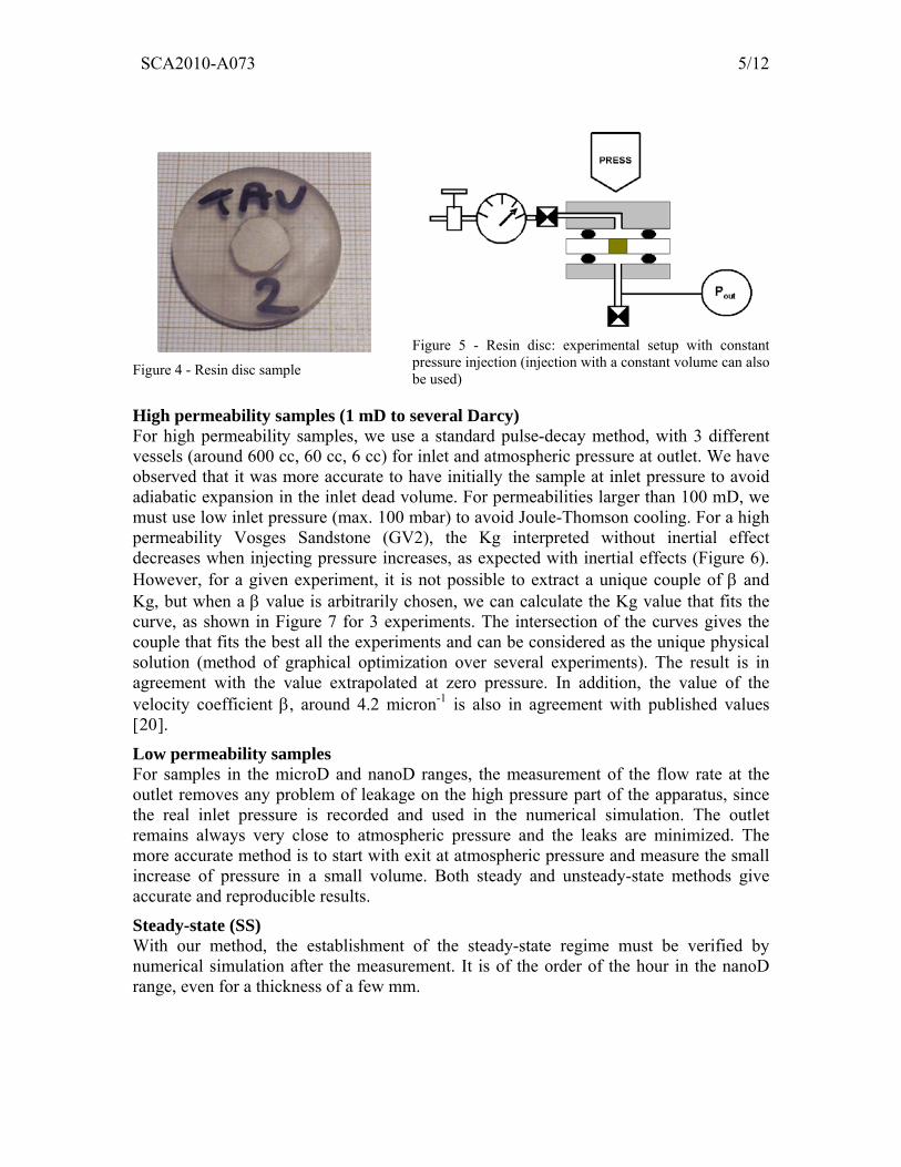
Small cylinders are sometimes taken from cores or small samples, mainly for microscanner studies (diameter 5 mm, length around 1 cm). These samples have generally a good permeability since the visualization requires large pores. Micro Hassler cells can be realized [19], but the faster technique to measure the permeability without destroying the sample is to put them into a silicon tube and perform a standard steady-state or pulse-decay permeability measurement (Figure 2). The sealing between the tube and the core can be improved by using an additional shrinkable sleeve. The only constraint is to use low pressure in order to avoid leaks between the sample and the silicon tube. We have performed experiments with a maximum pressure of 100 mbar that leads to reproducible results comparable to core permeability. A Fontainebleau sandstone with permeability of 2.5 Darcy measured with a micro Hassler cell gives 5 Darcy on a miniplug with only silicone tube (Figure 3) and 4.8 Darcy with additional shrinkable sleeve (the difference with core can be due to core heterogeneity). RESIN DISCS However, it is difficult to plug a cylinder from a small sample and it is easier to make a disc embedded in resin. For permeabilities larger than 1 mD, a first coating is done with a high viscosity resin to prevent the invasion of pores. For lower permeabilities, a low viscosity resin allows the partial invasion over a small distance and a good sealing. Once embedded in resin, the sample is cut in a slice (1 to 5 mm) and the faces are polished. (Figure 4). The resin disc is placed between two end pieces (Figure 5). The tightness is ensured by applying a load using a hydraulic press. The entry can be connected to several vessels of different volumes. The outlet is open to the atmosphere or closed on a small volume. Inlet and outlet pressures are measured. This setup allows unsteady-state and steady-state gas flow experiments.

SCA2010-A073 5/12

Figure 4 - Resin disc sample

Figure 5 - Resin disc: experimental setup with constant pressure injection (injection with a constant volume can also be used)

High permeability samples (1 mD to several Darcy) For high permeability samples, we use a standard pulse-decay method, with 3 different vessels (around 600 cc, 60 cc, 6 cc) for inlet and atmospheric pressure at outlet. We have observed that it was more accurate to have initially the sample at inlet pressure to avoid adiabatic expansion in the inlet dead volume. For permeabilities larger than 100 mD, we must use low inlet pressure (max. 100 mbar) to avoid Joule-Thomson cooling. For a high permeability Vosges Sandstone (GV2), the Kg interpreted without inertial effect decreases when injecting pressure increases, as expected with inertial effects (Figure 6). However, for a given experiment, it is not possible to extract a unique couple of β and Kg, but when a β value is arbitrarily chosen, we can calculate the Kg value that fits the curve, as shown in Figure 7 for 3 experiments. The intersection of the curves gives the couple that fits the best all the experiments and can be considered as the unique physical solution (method of graphical optimization over several experiments). The result is in agreement with the value extrapolated at zero pressure. In addition, the value of the velocity coefficient β, around 4.2 micron-1 is also in agreement with published values [20].

Low permeability samples For samples in the microD and nanoD ranges, the measurement of the flow rate at the outlet removes any problem of leakage on the high pressure part of the apparatus, since the real inlet pressure is recorded and used in the numerical simulation. The outlet remains always very close to atmospheric pressure and the leaks are minimized. The more accurate method is to start with exit at atmospheric pressure and measure the small increase of pressure in a small volume. Both steady and unsteady-state methods give accurate and reproducible results.

Steady-state (SS) With our method, the establishment of the steady-state regime must be verified by numerical simulation after the measurement. It is of the order of the hour in the nanoD range, even for a thickness of a few mm.

SCA2010-A073 6/12

0

1

2

3

4

5

0 0.05 0.1 0.15pressure (bar)

perm

eabi

lity

(Dar

cy)

GV20

1

2

3

4

5

0 0.05 0.1 0.15pressure (bar)

perm

eabi

lity

(Dar

cy)

GV2

Figure 6 – Sample GV2: permeability without inertial effect as function of injection pressure. The Kg extrapolated at zero pressure is 4.5 Darcy

2

3

4

5

6

0 2 4 6β (1/micron)

Kg

(Dar

cy)

114 mbar14 mbar67 mbar

GV2

2

3

4

5

6

0 2 4 6β (1/micron)

Kg

(Dar

cy)

114 mbar14 mbar67 mbar

GV2

Figure 7 – Sample GV2: interpretation with inertial effects with the best Kg for various values of β. The intersection of the curves gives the couple β, Kg that is the optimum for the different experiments

The gas permeability is derived from pressure and flow rate assuming Boyle's law for compressibility. Results on several samples verify the standard linear Klinkenberg relationship both in the nanoD (Figure 8) and microD ranges (Figure 9) at high pressure. However, below 100 mbar the behavior is no longer linear, as already described in several publications [21]. Figure 10 shows the example of GOS sample with the last point obtained using vacuum.

0

100

200

300

0.0 0.5 1.0

1/<P> (1/bar)

Kg

(nan

oD) AT1

GOS

0

100

200

300

0.0 0.5 1.0

1/<P> (1/bar)

Kg

(nan

oD) AT1

GOS

Figure 8 – Linear Klinkenberg corrections for AT1 and GOS samples from steady-state measurements

0

20

40

60

80

0.0 0.5 1.0

1/<P> (1/bar)

Kg

(mic

roD

)

LAV

MOL

TAV

0

20

40

60

80

0.0 0.5 1.0

1/<P> (1/bar)

Kg

(mic

roD

)

LAV

MOL

TAV

Figure 9 - Linear Klinkenberg corrections for LAV, MOL and TAV samples from steady-state measurements

Unsteady-state (USS) The USS method presents the advantage to allow (at least in theory) the simultaneous determination of both Kl and b on a single experiment. The sample is initially at atmospheric pressure and the outlet small volume is closed. The inlet pressure is slowly increased to minimize any temperature change due to adiabatic compression. The output and input pressures are then recorded. The outlet pressure shows a delay before starting to increase, due to the accumulation of gas inside the sample (Figure 11).

SCA2010-A073 7/12

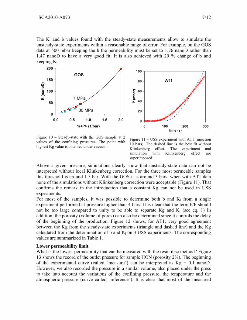
The Kl and b values found with the steady-state measurements allow to simulate the unsteady-state experiments within a reasonable range of error. For example, on the GOS data at 500 mbar keeping the b the permeability must be set to 1.76 nanoD rather than 1.47 nanoD to have a very good fit. It is also achieved with 20 % change of b and keeping Kl.

0

50

100

150

200

0.0 0.5 1.0 1.5 2.01/<P> (1/bar)

K (n

anoD

)

7 MPa

30 MPa

GOS

0

50

100

150

200

0.0 0.5 1.0 1.5 2.01/<P> (1/bar)

K (n

anoD

)

7 MPa

30 MPa0

50

100

150

200

0.0 0.5 1.0 1.5 2.01/<P> (1/bar)

K (n

anoD

)

7 MPa

30 MPa

GOS

Figure 10 – Steady-state with the GOS sample at 2 values of the confining pressures. The point with highest Kg value is obtained under vacuum.

0

20

40

60

80

100

0 100 200 300time (s)

P (m

bar)

AT1

0

20

40

60

80

100

0 100 200 300time (s)

P (m

bar)

AT1

Figure 11 – USS experiment with AT1 (injection 10 bars). The dashed line is the best fit without Klinkenberg effect. The experiment and simulation with Klinkenberg effect are superimposed

Above a given pressure, simulations clearly show that unsteady-state data can not be interpreted without local Klinkenberg correction. For the three most permeable samples this threshold is around 1.5 bar. With the GOS it is around 3 bars, when with AT1 data none of the simulations without Klinkenberg correction were acceptable (Figure 11). That confirms the remark in the introduction that a constant Kg can not be used in USS experiments. For most of the samples, it was possible to determine both b and Kl from a single experiment performed at pressure higher than 4 bars. It is clear that the term b/P should not be too large compared to unity to be able to separate Kg and Kl (see eq. 1) In addition, the porosity (volume of pores) can also be determined since it controls the delay of the beginning of the production. Figure 12 shows, for AT1, very good agreement between the Kg from the steady-state experiments (triangle and dashed line) and the Kg calculated from the determination of b and Kl on 3 USS experiments. The corresponding values are summarized in Table 1.

Lower permeability limit What is the lowest permeability that can be measured with the resin disc method? Figure 13 shows the record of the outlet pressure for sample HON (porosity 2%). The beginning of the experimental curve (called "measure") can be interpreted as Kg = 0.1 nanoD. However, we also recorded the pressure in a similar volume, also placed under the press to take into account the variations of the confining pressure, the temperature and the atmospheric pressure (curve called "reference"). It is clear that most of the measured

SCA2010-A073 8/12

pressure follows the reference. The difference between reference and measure presents a small trend but is not considered as significant. The limit of the equipment is considered around 0.1 nanoD, corresponding to the straight line on the figure. We recall that atmospheric pressure can vary by several mbar during one hour and that a temperature change of 1°C corresponds to 3 mbar.

0

50

100

150

0 0.2 0.41/P (1/bar)

Kg

(nan

oD)

AT1

0

50

100

150

0 0.2 0.41/P (1/bar)

Kg

(nan

oD)

AT1

Figure 12 – AT1 sample. The triangles and dashed line are from steady-state, the other lines are the Klinkenberg local lines from unsteady-states

Table 1 – AT1: Liquid permeability Kl and Klinkenberg coefficient from SS and USS experiments

porosity b Kl

SS - 262 8.8 USS 4.3 bar 0.112 228 1.25

USS 6.7 bar 0.112 92 3.08

USS 10 bar 0.114 103 2.9

measure

reference

difference

0.1 nD

HON measure

reference

difference

0.1 nD

measure

reference

difference

0.1 nD

HON

Figure 13- Sample HON showing the comparison between the measured and reference pressures. The permeability is below the threshold of the equipment estimated at 0.1 nanoD (straight line)

0

0.2

0.4

0.6

0.8

1

1.2

0.0 0.2 0.4 0.6 0.81/<P> (1/bar)

Kg

stea

dy (m

icro

D)

14 MPa ↓

40 MPa ↑

28 MPa ↑

7 MPa ↑

0

0.2

0.4

0.6

0.8

1

1.2

0.0 0.2 0.4 0.6 0.81/<P> (1/bar)

Kg

stea

dy (m

icro

D)

14 MPa ↓

40 MPa ↑

28 MPa ↑

7 MPa ↑

Figure 14 – Sample SB: effect of the stress applied on the disc. Pressure applied on the disc is increased (↑) at 7, 28, 40 MPa and then decreased (↓) at 14 MPa

Effect of stress The set up allows to apply a stress on the disc. For most of the experiments, we have applied a low force, just enough for sealing (70 MPa). It was not the purpose of the study, but we have also run some experiments with increasing and decreasing the stress on sample SB (argilite). As expected, the permeability decreases when stress increases, with some hysteresis when stress is reduced. A study will be performed to show how this stress can be compared to a confining pressure on a core.

SCA2010-A073 9/12

OPEN SURFACE WITH LIQUID This technique was developed by IFP for drill cuttings under the name of Darcylog [22]. The principle is to achieve an effective flow of a viscous liquid inside the cuttings by compression of the residual gas that they contain. The size of the grains is between 1 and 5 mm and the total volume of rock is around 5 cc. This method enables measurement of permeabilities corresponding to reservoir rocks in the range 0.05 to 100 mDarcy, depending on the porosity and the size of the cuttings. OPEN SURFACE WITH GAS (PDOS)

8.75

8.8

8.85

8.9

8.95

0 5 10 15 20time (s)

pres

sure

Abs

(mba

r)

MOL

8.75

8.8

8.85

8.9

8.95

0 5 10 15 20time (s)

pres

sure

Abs

(mba

r)

MOL

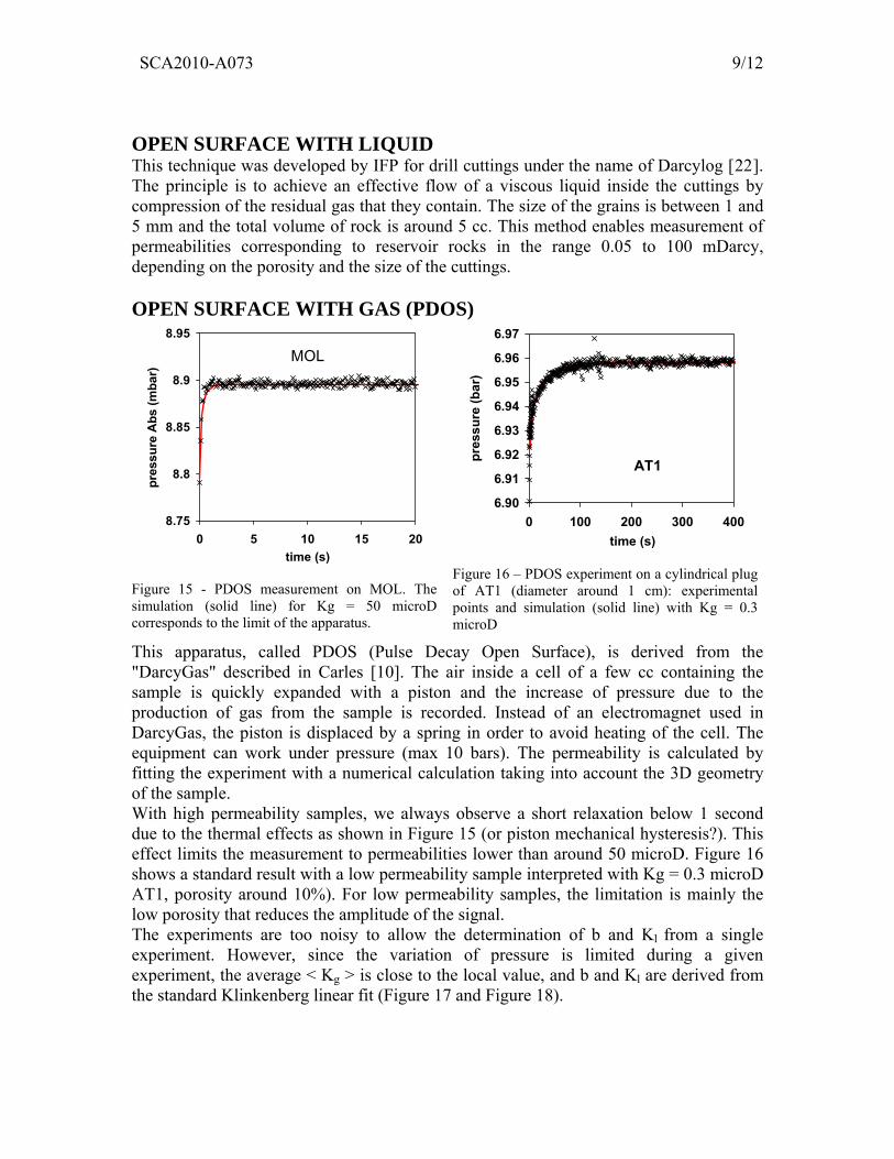
Figure 15 - PDOS measurement on MOL. The simulation (solid line) for Kg = 50 microD corresponds to the limit of the apparatus.

6.90

6.91

6.92

6.93

6.94

6.95

6.96

6.97

0 100 200 300 400time (s)

pres

sure

(bar

)AT1

6.90

6.91

6.92

6.93

6.94

6.95

6.96

6.97

0 100 200 300 400time (s)

pres

sure

(bar

)AT1

Figure 16 – PDOS experiment on a cylindrical plug of AT1 (diameter around 1 cm): experimental points and simulation (solid line) with Kg = 0.3 microD

This apparatus, called PDOS (Pulse Decay Open Surface), is derived from the "DarcyGas" described in Carles [10]. The air inside a cell of a few cc containing the sample is quickly expanded with a piston and the increase of pressure due to the production of gas from the sample is recorded. Instead of an electromagnet used in DarcyGas, the piston is displaced by a spring in order to avoid heating of the cell. The equipment can work under pressure (max 10 bars). The permeability is calculated by fitting the experiment with a numerical calculation taking into account the 3D geometry of the sample. With high permeability samples, we always observe a short relaxation below 1 second due to the thermal effects as shown in Figure 15 (or piston mechanical hysteresis?). This effect limits the measurement to permeabilities lower than around 50 microD. Figure 16 shows a standard result with a low permeability sample interpreted with Kg = 0.3 microD AT1, porosity around 10%). For low permeability samples, the limitation is mainly the low porosity that reduces the amplitude of the signal. The experiments are too noisy to allow the determination of b and Kl from a single experiment. However, since the variation of pressure is limited during a given experiment, the average < Kg > is close to the local value, and b and Kl are derived from the standard Klinkenberg linear fit (Figure 17 and Figure 18).

SCA2010-A073 10/12

DISCUSSION The comparison of the different methods is quite difficult due to the lack of reference samples for low permeability and the heterogeneity of the samples at different scales. We will continue the comparisons, but so far we have the following conclusions:

0

200

400

600

800

1000

0 0.2 0.4 0.61/P (1/bar)

Kg

(nan

oD)

PDOS

Disc

AT1

0

200

400

600

800

1000

0 0.2 0.4 0.61/P (1/bar)

Kg

(nan

oD)

PDOS

Disc

AT1

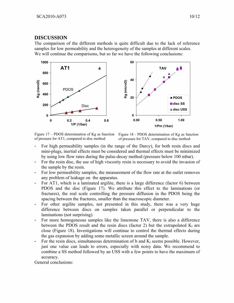
Figure 17 – PDOS determination of Kg as function of pressure for AT1, compared to disc method

0

20

40

60

0.00 0.50 1.00

1/Pm (1/bar)K

g (m

icro

D)

PDOS

disc SS

disc USS

TAV

0

20

40

60

0.00 0.50 1.00

1/Pm (1/bar)K

g (m

icro

D)

PDOS

disc SS

disc USS

TAV

Figure 18 - PDOS determination of Kg as function of pressure for TAV, compared to disc method

- For high permeability samples (in the range of the Darcy), for both resin discs and mini-plugs, inertial effects must be considered and thermal effects must be minimized by using low flow rates during the pulse-decay method (pressure below 100 mbar).

- For the resin disc, the use of high viscosity resin is necessary to avoid the invasion of the sample by the resin.

- For low permeability samples, the measurement of the flow rate at the outlet removes any problem of leakage on the apparatus.

- For AT1, which is a laminated argilite, there is a large difference (factor 6) between PDOS and the disc (Figure 17). We attribute this effect to the laminations (or fractures), the real scale controlling the pressure diffusion in the PDOS being the spacing between the fractures, smaller than the macroscopic diameter.

- For other argilite samples, not presented in this study, there was a very huge difference between discs on samples taken parallel or perpendicular to the laminations (not surprising).

- For more homogeneous samples like the limestone TAV, there is also a difference between the PDOS result and the resin discs (factor 2) but the extrapolated Kl are close (Figure 18). Investigations will continue to control the thermal effects during the gas expansion by adding some metallic screen around the sample.

- For the resin discs, simultaneous determination of b and Kl seems possible. However, just one value can leads to errors, especially with noisy data. We recommend to combine a SS method followed by an USS with a few points to have the maximum of accuracy.

General conclusions:

SCA2010-A073 11/12

- The importance of the thermal effects can be prevented by using slow changes of pressures when possible.

- The linear "Klinkenberg" law seems quite robust, even at very low permeabilities (except at very low pressure). However, this is a "local" law and its integration to a similar "macroscopic" law is only valid for a steady state flow.

- All the interpretations require specific numerical calculation, taking into account the local Klinkenberg and inertial laws, various boundary conditions (like a pressure ramp) and various initial conditions (USS following a SS).

Figure 19 shows the domains of utilization of the methods described in this paper:

nanoD microDK

milliD Darcy

1 mm

5 mm

1 cm

Sample size

Resin disc

Darcylog

PDOS

nanoD microDK

milliD Darcy

1 mm

5 mm

1 cm

Sample size

nanoD microDK

milliD Darcy

1 mm

5 mm

1 cm

Sample size

Resin disc

Darcylog

PDOS

Figure 19 – Schematic diagram of the domains of application of the various techniques

- the resin disc needs a sample of size 5mm to be able to cut a final slice of 1-2 mm. The minimum permeability is around 0.1 nanoD. There is no constraint on porosity.

- the Darcylog method is limited to small grains (below 5mm) to allow the spontaneous imbibition with a viscous fluid, but larger sample can be crushed. The lower limit is around 50 microD due to fast dissolution of air trapped in the small pores, under the action of high capillary pressure.

- the PDOS requires big samples with low permeabilities.

ACKNOWLEDGEMENTS We thank IFP for providing some of the samples used in this study. REFERENCES

1 Siddiqui S., Grader A.S., Touati M., Loermans A.M., Funk, J.J, " Techniques for extracting reliable density and porosity data from cuttings", SPE 96918 presented at ATCE,2005.

2 Desmette S., Deschamps B., Birch R., "Drilling hard and abrasive rock efficiently, or generating quality cuttings? You no longer have to choose…", SPE 116554, 2008.

3 Deschamps B., Desmette S., Delwiche R., Birch R., Azhar J., Naoegel M., Essel P., "Drilling to the Extreme: the Micro-Coring Bit Concept", SPE 115187, 2008.

4 Egermann, P., Doerler, N., Fleury, M., Behot, J. Deflandre, F.and Lenormand, R., "Petrophysical measurements from drill cuttings: an added value for the reservoir characterization processes", SPE 88684, published in SPE Reservoir Evaluation and Engineering, August, 303-307, 2006.

5 Lenormand R., Fonta O., "Advances in Measuring Porosity and Permeability from Drill Cuttings", SPE 111286, 2007.

SCA2010-A073 12/12

6 Knackstedt, M.A., C.H. Arns, A. Limaye, C.H. Arns, A. Limaye, A. Sakellariou,

T.J. Senden, A.P. Sheppard, R.M. Sok, W.V. Pinczewski, and G.F. Bunn: "Digital core laboratory: Reservoir-core properties derived from 3D images," Journal of Petroleum Technology, 56, 66-68, 2004.

7 Santarelli, F. J., A. F. Marsala, M. Brignoli et al.: “Formation evaluation from logging on cuttings”, SPEREE, 238-244. 1998.

8 Luffel, D. L.,"Devonian shale matrix permeability successfully measured on cores and drill cuttings", Gas Shales Technology Review, 8, No 2, 46-55, 1993.

9 Luffel D.L., Hopkins C.W., and Shettler, P.D., "Matrix Permeability Measurements of Gas Productive Shales", SPE 26633, 1993;

10 Carles P. , Egermann P., Lenormand R. , Lombard J.M., " low permeability measurements using steady state and transient methods, SCA A32, 2007.

11 API, "Recommended Practices for Core Analysis", Recommended Practice 40, second Edition, February 1998.

12 Jannot Y., Lasseux D., Vizé G., Hamon G., "A detailed analysis of permeability and Klinkenberg coefficient estimation from unsteady-state pulse-decay or draw-down experiments", SCA08, 2007.

13 Ma H., Ruth D., "The microscopic analysis of high Forchheimer number flow in porous media", Transport in Porous Media, vol 13, 139-160, 1993.

14 Fourar M., Radilla G., Lenormand R. Moyne C., "On the non-linear behavior of a laminar single-phase flow through two and three-dimensional porous media", Advances in Water resources, Vol. 27, 669-677, 2004,

15 Scott, D.S. and Dullien F.A.L.: “Diffusion of Ideal Gases in Capillaries and Porous Solids" A.I.Ch.E. Journal, V.8, p.113-117, 1962.

16 Rushing J.A., Newsham K.E., Lasswell P.M., Cox J.C., Blasingame T., "Klinkenberg-Corrected Permeability Measurements in Tight Gas Sands: Steady-State Versus Unsteady-State Techniques", SPE 89867, 2004.

17 Maloney D., Briceno M., "Experimental investigation of cooling effects resulting from injecting high pressure liquid or supercritical CO2 into a low pressure resevoir", SCA40, 2008.

18 Mage D., Katz D., " Enthalpy determinations on the helium-nitrogen system", A.I.Ch.E. Journal, vol. 12, n° 1, 1966.

19 Youssef S. Bauer D.; Bekri S.; Rosenberg E.; Vizika O., " Towards a better understanding of multiphase flow in porous media: 3D in-situ fluid distribution imaging at the pore scale", SCA A17, 2009.

20 Firoozabadi A., Katz, D., "An analysis of high-velocity gas flow through porous media,", Journal of Petroleum Technology, 1979.

21 Grove, D. M. & Ford M. G. , "Evidence for permeability minima in low-pressure gas flow through porous media". Nature 182, 999–1000, 1958.

22 Egermann P., Lenormand R., Longeron D., and Zarcone C.: "A Fast and Direct Method of Permeability Measurements on Drill Cuttings", SPE Reservoir Evaluation & Engineering, p. 269-275, 2005.