permanent magnet work at fermilab 1995 to...
TRANSCRIPT

Permanent Magnet Work at
Fermilab
1995 to Present
James T Volk
Applications Physicist II
Fermilab Accelerator Division

Klaus Halbach
1924 to 2000
Halbach made his reputation with his work on
magnetic systems for particle accelerators. He and
Ron Holsinger a Berkley engineer created the
famous POISSON computer codes for magnetic
system design, still in use after 30 years. Halbach
went on to become one of the world’s premier
designers and developers of permanent magnets for
use as insertion devices- wigglers and undulators in
synchrotron light sources and free electron lasers.
He also designed the magnets for the Berkeley
Advanced Light Source storage ring.
Klaus Halbach
2James T Volk Fermilab
Fermilab Contributors
James T Volk Fermilab 3
There were a large number of people at Fermilab that
worked on permanent magnets and the Recycler.
There were many other including;
KJ Bertsche, BC Brown, CN Brown, J DiMarco, WB Fowler,
HD Glass, DJ Harding, V Kashikin, MP May, TH Nicol, J-F
Ostiguy, S Pruss plus many others
Bill Foster and Gerry Jackson
were the first to conceive of the Recyler and push it to a successful conclusion

Layout of Talk
• Fundamental definitions
• Types of permanent magnets
• Temperature compensation
• Radiation damage
• Time dependence
• The 8 GeV transfer line at Fermilab
• The Recycler at Fermilab
• Adjustable Permanent Magnet Quadrupoles for the NLC
• Other permanent magnets
James T Volk Fermilab 4

Sources of Information
• If you Google permanent magnets get 1,560,000 results -some of the better
ones are:
• For theory Ferromagnetism by Richard Bozorth IEEE press
• For a how to guide International Magnetics Association
– http://www.intl-magnetics.org/
• Papers on the Fermilab Recycler can be found in PAC 95, 97, 99, 2000 and 2003
• Dexter Magnetics
– http://www.dextermag.com/
• Ugimag
– http://www.ugimag.com/
• Hitachi
– http://www.hitachimetals.com/product/permanentmagnets/
James T Volk Fermilab 5

Important Definitions
• B residual Br The magnetic induction after saturation in a closed circuit
• Remnant induction Bd The magnetic induction that remains after the removal of an applied
field
• Hd is the value of H corresponding to Bd on the demagnetization curve
• Intrinsic Coercive Force Hci indicates its resistance to demagnetization
• On a hysteresis curve of B vs H the Br is where Hci is 0 and the Hci is where Br is 0
• Load line has a slope equal to - Bd / Hd and is drawn in the 2nd quadrant
• The product of Bd and Hd is the measure of how much energy can be supplied to the circuit
and is measured in Mega Gauss Oersteds (MGO)
• The Curie temperature Tc is the temperature that the material demagnetizes
• Easy axis this is the direction of the field in the material
• A Fermilab Unit is Measured Field / Ideal Field * 104
James T Volk Fermilab 6

Types of Magnetic Material
James T Volk Fermilab 7
Strontium Ferrite
Hard ceramic
Inexpensive
Br 3800 Gauss
Energy density 3.5 MegaGauss Oersteds
Samarium Cobalt
Rare earth
Expensive
Br 9000 to 10,000 gauss
Energy density 26 MegaGauss Oersteds
Neodymium Iron Boron
Rare earth
Expensive
Br 11,000 to 12,000 gauss
Energy Density 35 to 50 MegaGauss Oersteds
Alnico
Metal
Inexpensive
Br 3,000 to 5,000 Gauss
Energy density 7 MegaGauss Oersteds
Load Line for a Simple Dipole
James T Volk Fermilab 8
ℓgℓm
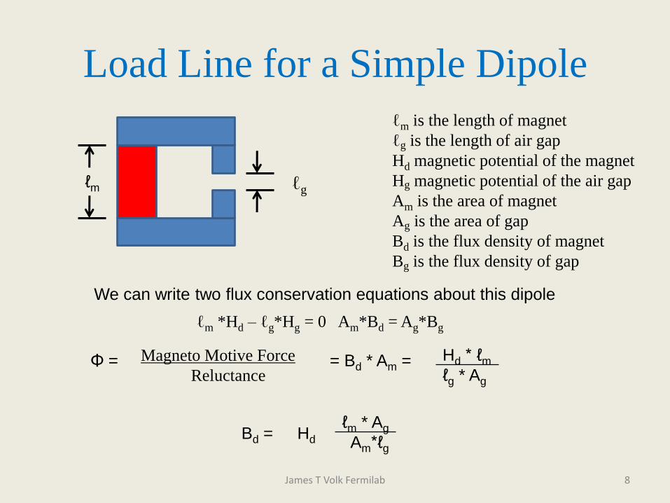
ℓm *Hd – ℓg*Hg = 0 Am*Bd = Ag*Bg
ℓm is the length of magnet
ℓg is the length of air gap
Hd magnetic potential of the magnet
Hg magnetic potential of the air gap
Am is the area of magnet
Ag is the area of gap
Bd is the flux density of magnet
Bg is the flux density of gap
Magneto Motive Force
ReluctanceΦ = = Bd * Am =
We can write two flux conservation equations about this dipole
Hd * ℓm
ℓg * Ag
Bd = ℓm * Ag
Am*ℓgHd

Load Line
James T Volk Fermilab 9
Bd /Hd = ℓm * Ag
Am * ℓgThis is the slope
It is important to stay away from
the knee of the curve.
B in Tesla
H in Kilo Oersteds
Load Line The different curves are
for different grades of
material
Energy Density

Magnet Modeling Software
• There are many different magnet modeling programs available
– ANSYS
– Ansoft MAXWELL
– Vector Fields OPERA and TOSCA
– POISSON and PANDRIA
James T Volk Fermilab 10
•I use POISSON and PANDRIA
–They are simple and free available from Los Alamos code group
– http://laacg1.lanl.gov/laacg/services/download_sf.phtml
–Jim Billen and the Los Alamos code group has made a WINDOWS version
–They do 2 dimensional models very quickly and accurately
–Creates triangular mesh that can be densified in areas of interest
–Allow for different material steel and permanent magnets
–Graphical output helps to visualize program–Can calculate harmonics
-Can be installed and working in less than 1 hour
Free Magnet and a Hallbach Array
of the same size
James T Volk Fermilab 11
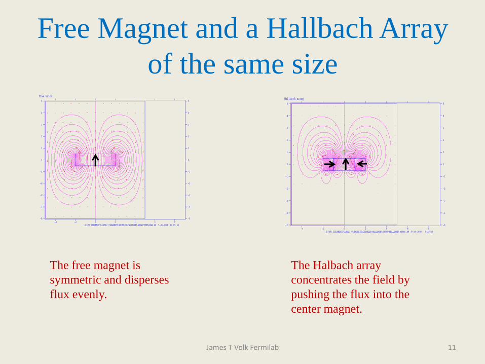
The Halbach array
concentrates the field by
pushing the flux into the
center magnet.
The free magnet is
symmetric and disperses
flux evenly.

Halbach Array
James T Volk Fermilab 12
This is a simple
array of three
magnets.
The black arrows
indicate the
direction of the
easy axis.
The two outside
magnets are
pushing flux
into the center
magnet.

Sample POISSON Input for Halbach Array
James T Volk Fermilab 13
Hallbach array
Original version from the 1987 User's Guide, Chapter 10.5
First pass simple 3 ferrite magnet Halbach array
; Copyright 1998, by the University of California.
; Unauthorized commercial use is prohibited.
® kprob=0, ; Defines a POISSON or PANDIRA problem
conv = 2.54, ; inches
dx = 0.05 ; mesh size
dy = 0.05 ; mesh size
nbslo = 0, ; Dirchelt boundary condtion at bottom
ktype = 1, ; symmetry midplane for this
nterm = 11, ; number of harmonics terms
nptc = 1440, ; number of arc points
rint = 0.4, ; radius to calculate harmonics
angle = 360.0, ; angle to calculate harmonics
mode=0 & ; Materials have variable permeability
&po x= -5.0, y = -5.0 & ;entire universe
&po x= 5.0, y = -5.0 &
&po x= 5.0, y = 5.0 &
&po x= -5.0, y = 5.0 &
&po x= -5.0, y = -5.0 &
® mat=6,mshape=1,mtid=6 & ; RHS magnet
&po x = 1.000, y = -0.500 &
&po x = 2.000, y = -0.500 &
&po x = 2.000, y = 0.500 &
&po x = 1.000, y = 0.500 &
&po x = 1.000, y = -0.500 &
® mat=8,mshape=1,mtid=4 & ;Center magnet
&po x = -1.000, y = -0.500 &
&po x = 1.000, y = -0.500 &
&po x = 1.000, y = 0.500 &
&po x = -1.000, y = 0.500 &
&po x = -1.000, y = -0.500 &
® mat=7,mshape=1,mtid=2 & ; LHS magnet
&po x = -1.000, y = -0.500 &
&po x = -2.000, y = -0.500 &
&po x = -2.000, y = 0.500 &
&po x = -1.000, y = 0.500 &
&po x = -1.000, y = -0.500 &
&mt mtid=2,aeasy= 0,gamper=1,hcept=-3500,bcept=3800. & ; Sr Ferrite
&mt mtid=4,aeasy= 90,gamper=1,hcept=-3500,bcept=3800. & ; Sr Ferrite
&mt mtid=6,aeasy= 180,gamper=1,hcept=-3500,bcept=3800. & ; Sr Ferrite

Halbach Array Dipole
James T Volk Fermilab 14
Two Halbach arrays used to make
a simple dipole.
Note the change in the easy axis
for the side magnets.
The addition of steel on the top
and sides increases the field in
the gap by 32%. Again the
black arrows are the easy axis.

Halbach Array Quadrupole
James T Volk Fermilab 15
This is two Halbach
arrays facing each
other to make a
quadrupole field.
Adding flux returns
increases flux by 21%
Halbach Array Sextupole
James T Volk Fermilab 16
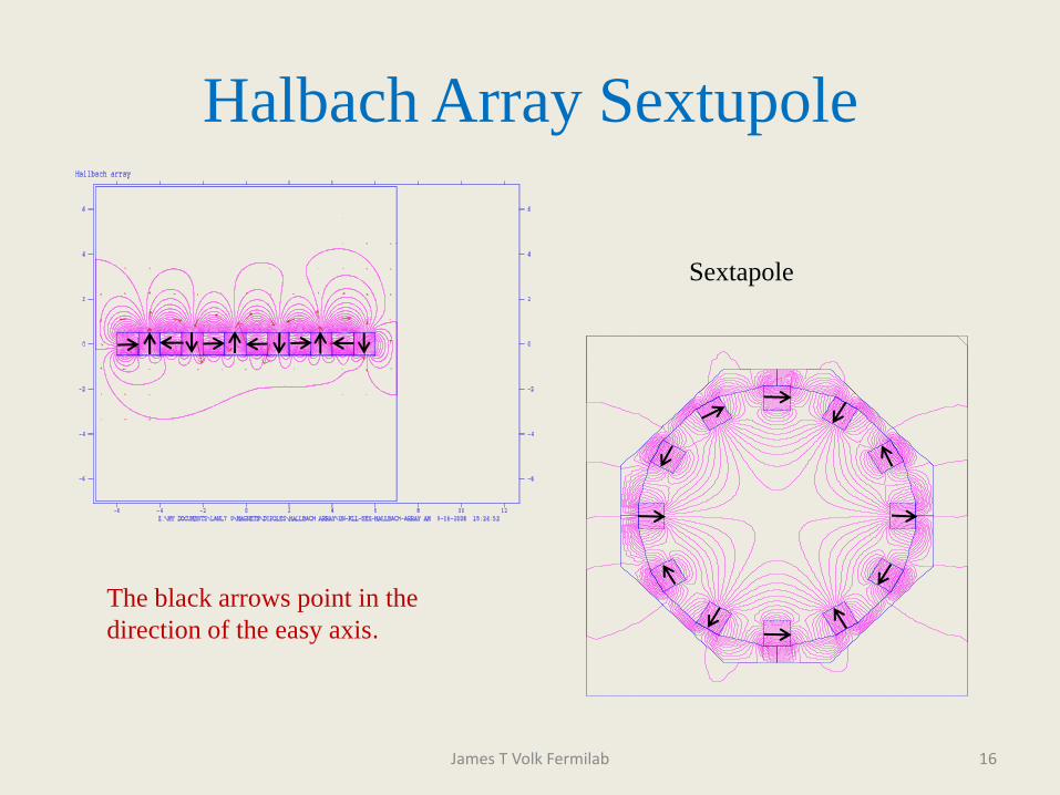
The black arrows point in the
direction of the easy axis.
Sextapole

Temperature Variation
James T Volk Fermilab 17
The magnetic field Br
varies with temperature.
For Sr Ferrite the
variation is 0.18%
per degree C.
For Samarium Cobalt
the variation is 0.11%
per degree C. This is a plot of Temperature vs
gradient strength for a recycler quad.
The field falls off 720 units over a 40
C temperature change.
As the magnets get hotter
the Br decreases.

Temperature Compensation
James T Volk Fermilab 18
The solution is to use steel with
28% Nickel added. The Tc (Curie
temperature) of the steel is 55 C.
The material is placed between the
pole pieces and the flux return.
Ferrite
Compensator steel
As the temperature decreases
the µ of the steel increases and acts like
an iron shunt removing flux from the
gap. As the temperature increase the µ
goes to unity and acts like air allowing
more flux into the gap.
Empirically determine the correct
ratio compensator steel to ferrite.
This varies from batch to batch.

Temperature Compensated Magnet
James T Volk Fermilab 19
This has undergone a 5
degree C temperature
change.
A n un compensated
magnet would change
by 90 units.
This magnet changes
by 0.7 units.

Radiation Damage
James T Volk Fermilab 20
Large amount of literature on radiation damage see
http://www-project.slac.stanford.edu/lc/local/notes/dr/Wiggler/wiggler_rad.html
Many different types of exposures protons, neutrons, gammas
Many different manufactures and materials
No consistent results
All studies are on rare earth magnets

Demagnetization due to Radiation
James T Volk Fermilab 21
Demagnetization of REC
from F. Coninckx et. al.
-120
-100
-80
-60
-40
-20
0
0 5 10 15
dose *1E9 rads
% c
han
ge
Recoma 20
Vacomax 200
Koermax 160
all Sm Cobalt
magnet
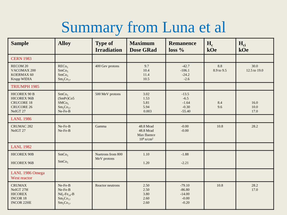
Summary from Luna et al
James T Volk Fermilab 22
Sample Alloy Type of
Irradiation
Maximum
Dose GRad
Remanence
loss %
Hc
kOe
Hci
kOe
CERN 1983
RECOM 20
VACOMAX 200
KOERMAX 60
Krupp WIDIA
RECo5
SmCo5
SmCo5
Sm2Co17
400 Gev protons 9.7
10.4
11.4
10.5
-42.7
-106.1
-24.2
-2.6
8.8
8.9 to 9.5
30.0
12.5 to 19.0
TRIUMPH 1985
HICOREX 90 B
HICOREX 96B
CRUCORE 18
CRUCORE 26
NeIGT 27
SmCo5
(SmPr)Co5
SMCo5
Sm2Co17
Ne-Fe-B
500 MeV protons 3.02
1.53
5.81
5.94
0.003
-13.5
-6.5
-1.64
-0.30
-55.40
8.4
9.6
16.0
10.0
17.0
LANL 1986
CRUMAC 282
NeIGT 27
Ne-Fe-B
Ne-Fe-B
Gamma 48.8 Mrad
48.8 Mrad
Max fluence
108 n/cm2
-0.00
-0.00
10.8 28.2
LANL 1982
HICOREX 90B
HICOREX 96B
SmCo5
SmCo5
Nuetrons from 800
MeV protons
1.10
1.20
-1.88
-2.21
LANL 1986 Omega
West reactor
CRUMAX
NeIGT 27H
HICOREX
INCOR 18
INCOR 22HE
Ne-Fe-B
Ne-Fe-B
Nd2-Fe14-B
Sm2Co17
Sm2Co17
Reactor neutrons 2.50
2.50
3.80
2.60
2.60
-79.10
-86.80
-14.00
-0.00
-0.20
10.8 28.2
17.0
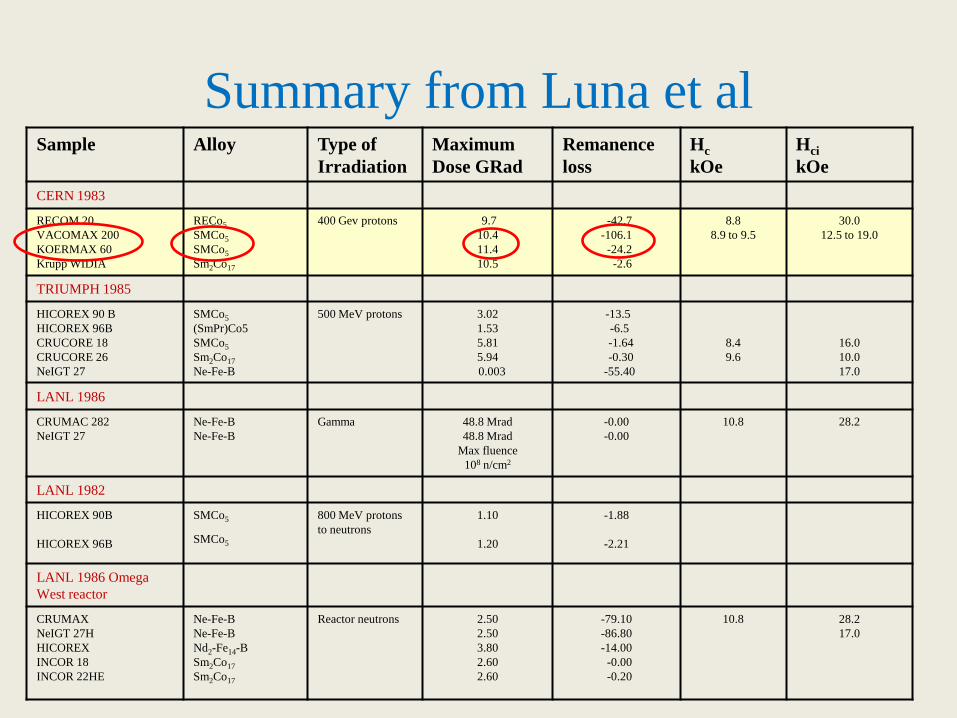
Summary from Luna et al
James T Volk Fermilab 23
Sample Alloy Type of
Irradiation
Maximum
Dose GRad
Remanence
loss
Hc
kOe
Hci
kOe
CERN 1983
RECOM 20
VACOMAX 200
KOERMAX 60
Krupp WIDIA
RECo5
SMCo5
SMCo5
Sm2Co17
400 Gev protons 9.7
10.4
11.4
10.5
-42.7
-106.1
-24.2
-2.6
8.8
8.9 to 9.5
30.0
12.5 to 19.0
TRIUMPH 1985
HICOREX 90 B
HICOREX 96B
CRUCORE 18
CRUCORE 26
NeIGT 27
SMCo5
(SmPr)Co5
SMCo5
Sm2Co17
Ne-Fe-B
500 MeV protons 3.02
1.53
5.81
5.94
0.003
-13.5
-6.5
-1.64
-0.30
-55.40
8.4
9.6
16.0
10.0
17.0
LANL 1986
CRUMAC 282
NeIGT 27
Ne-Fe-B
Ne-Fe-B
Gamma 48.8 Mrad
48.8 Mrad
Max fluence
108 n/cm2
-0.00
-0.00
10.8 28.2
LANL 1982
HICOREX 90B
HICOREX 96B
SMCo5
SMCo5
800 MeV protons
to neutrons
1.10
1.20
-1.88
-2.21
LANL 1986 Omega
West reactor
CRUMAX
NeIGT 27H
HICOREX
INCOR 18
INCOR 22HE
Ne-Fe-B
Ne-Fe-B
Nd2-Fe14-B
Sm2Co17
Sm2Co17
Reactor neutrons 2.50
2.50
3.80
2.60
2.60
-79.10
-86.80
-14.00
-0.00
-0.20
10.8 28.2
17.0

Kähkönen et al. Jyväskylä Finland
Journal Phys Cond Mat 4 (1992)1007
Local heating of domains by knock atoms
Solve Laplace’s Equation
∂T/∂t = 2 T
Use a Green’s function to get
T = To + (Tc - To)(2 R2/3d2e-1)
Gives the heat needed to heat a radius R above the Curie temperature
The energy of a knock on atom is
Ekin = 3/2 kB (T1 - To)
An atom of material when hit will vibrate, it can flip direction If there is a
demagnetizing field present this will help to push it over. There is always some
demagnetizing filed present. It all depends on how the material was processed and
how big the grains are.
24James T Volk Fermilab

Radiation DamageUn-magnetized material Magnetized material arrows indicate direction of
field in each grain. Not all domains line up in each
grain In Rare earth magnets domain wall can move
in a grain
25James T Volk Fermilab
Arrows indicate direction of field in each grain.
Note a domain is 1015 atoms 0.1 micron or less
Grains are larger 1 micron or so

Test Quad Magnets
James T Volk Fermilab 26
Test quads with a gap of 2 mm
wide by 3 mm high able to fit into
Rabbit hole in McCellan Reactor
in Sacramento California.
Could vary load line by changing gap.
Irradiated different grades of
materials from different
manufacturers at the same time
and same flux.

From S Anderson et alNeutron irradiation at the McCellan reactor
James T Volk Fermilab 27
Alloy Manufacturer Mx
Gauss
dMx/dD
Gauss/Gray
SmCo HS36EH Hitachi 35 0.00
SmCo HS46AH Hitachi 128 -4.65
Ne-Fe-B N34Z1 Shin Etsu 266 -0.11
Ne-Fe-B N50M1 Shin Etsu 17 -2.28
What we found by looking at radioactive half lives
was many different doping elements
Rare Earth Elements such as Tb, Pm, Pr, Dy all
in different quantities for different manufactures
This work was stopped when the decision was made to
use superconducting RF

Practical Radiation Damage
• Strontium Ferrite is good to 109 Grays
• Rare Earths are harder to characterize
– Different manufactures add different materials
– It is important to understand what material is in the
magnets
– It is also important to test the magnets to ensure
that the material is what you expect
James T Volk Fermilab 28
Time Dependence
James T Volk Fermilab 29
In 1960 Konenberg and Bohlmann published in Journal of Applied
Physics Long Term Stability of Alnico and Barium Ferrite Magnets
ΔM = aTlog(t/t0)
Where t is time and T is absolute temperature
Theory developed by Louis Neel in 1950 and Street and Wooley in 1949
External shocks, temperature change can cause domains to flip thereby
decreasing the field.

Time Dependence of Fields
James T Volk Fermilab 30
This is a plot of Brel for the first
production gradient magnet vs. time.
From 1998 to 2002 the field has
decayed 0.2%. The decay is
logarithmic with time.
This is not enough to cause
problems with the recycler.

More Time dependence
James T Volk Fermilab 31
The same magnet premeasured
again in 2007 and 2008.
There has been no change in the RF in the recycler indicating no change
in the orbit and therefore no change in the field of the magnets

Over View of Fermilab Site
James T Volk Fermilab 32
Tevatron
Main Injector
And
Recycler
8 GeV Booster
8 Gev
Transfer line

8 Gev Transfer Line
Booster to Main Injector
James T Volk Fermilab 33
First proof of principle
that permanent magnets
work.
Beam transmitted on
third pulse.
No “beam line physicist”
assigned to the beam line.
45 Dipoles
65 Gradient magnets
9 Quadrupoles

Double Double Dipoles
James T Volk Fermilab 34
Pandria model of Double
Double dipole
Poles
Strontium Ferrite magnets
Temperature compensator
material
Position of side bricks
can change the sextupole
moment of the magnet

The Recycler
James T Volk Fermilab 35
Gerry Jackson and Bill Foster
In the Main Injector tunnel.
The Recycler is an 8.9 Gev/c
Anti proton storage ring in the
Main Injector tunnel 3.6 km
Circumference.
There are 488 permanent
Magnets in the ring.
362 Dipoles
109 Quadrupoles
8 Mirror magnets
5 Lambertson
4 Sextapoles

Design Parameters
• The lattice for the Recycler is the same as the Main Injector
• The aperture is 50.8 mm (2 inches) high and 88.9 mm (3.5 inches) wide
• ΔB/B = 1 x 10⁻⁴ or 1 unit over the 88.9 mm
• Hybrid design uses Strontium Ferrite magnets and steel poles tips
• Strontium Ferrite is cheaper than Alnico and Samarium Cobalt
• Sr Ferrite is readily available and is easily magnetized
• Gradient magnets were built to eliminate 82% of the separate Quadrupoles
• The poles were precision machined to give the proper gradient
• The flux returns were all bar stock with lower machining tolerance
James T Volk Fermilab 36
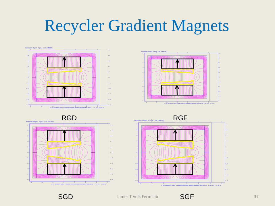
Recycler Gradient Magnets
James T Volk Fermilab 37
RGD RGF
SGD SGF

Recycler Parameters
James T Volk Fermilab 38
Type Total Pole
width
Pole
height
At center
Pole
length
B field Quadrupole Sextapole
units mm mm m Tesla units units
RGF 152 50.8 4.496 0.1375 619.7 8.7
RGD 152 50.8 4.496 0.1375 -598.1 -15.1
SGF 152 50.8 3.099 0.1330 1276.0 0.0
SGD 152 50.8 3.099 0.1330 -1303.1 0.0

Assembly
• Characterize batches of Strontium Ferrite magnets
– Test one box from skid to determine if weak or strong
• Magnetize Strontium Ferrite magnets
– Used old beam line dipole to provide the field built a transport system with PLU to drive
magnets in and out and ramp the dipole
• Devise stacking plan
– Changed the amount of Ferrite used in the magnets based on strong or weak magnets
• Place magnets on flux returns
– All magnets held in place mechanically not by epoxy
• Build on assembly table
– Needed for safe assembly of magnets
James T Volk Fermilab 39

The magnet factory
James T Volk Fermilab 40
Magnetizer
Test stand
Assembly
areaStorage

Assembly of a Gradient magnet
James T Volk Fermilab 41
Bottom plate
magnets and
compensator
Side plates
Ready to install
Pole assembly
On magnets
Top plate with
magnets
lower into
place

Assembly of Gradient
James T Volk Fermilab 42
Technicians
Cranking in
Side plates
Finished
Magnet
With traveler
Side plates
Ready to install

Field Measurements
James T Volk Fermilab 43
RGF 005 on test stand
at Magnet Test Facility
A Morgan coil was used to
measure field strength and
harmonics through 12 pole

Measure and Adjust Magnets
• Measure with a flip coil to check temperature compensation– Each magnet was frozen over night
– B field measured at 0 C and 22 C
– Compensation calculated
– Strips of compensator steel were added or subtracted
• Measured with Morgan coil to Adjust B field– Add or subtract magnetic material to achieve proper B field
– used pieces as small as ½” by ½” by 6”
• Tune harmonics– Use Morgan coil to measure harmonics through 12 pole
– Calculate shape of end shims to correct higher harmonics
– Bill Foster wrote a program that took data and generate machine code for wire EDM cut shims
directly
• Measured longitudinal field– Used hall probe on track to measure longitudinal field
James T Volk Fermilab 44

Brel and Normal Quad
James T Volk Fermilab 45
Histogram of
B measured/B ideal x 104
Specified 10 units
Held -6 + 8 units
Histogram of
Quad gradient
measured/ ideal x 104
Specified 619 2 units
Held 619 -1 +2 units

Higher Harmonics
James T Volk Fermilab 46
Normal Octopole
Specified 0 ± 1 units
Held 0 ± 0.5 units
Decapole
Specified 0 ± 1
Held 0 ± 0.5
Skew Sextapole
Specified 0 ± 1 units
Held 0 ± 1 units
Normal Sextapole
Specified 8 ± 1 units
Held 8 ± 1 units

Longitudinal field
James T Volk Fermilab 47
Even number of compensator
strips between each magnet.
Varied number of compensator
strips between each magnet
More strips close to center less at
the ends.

Recycler Quadrupoles
James T Volk Fermilab 48
PANDRIA model of the
Recycler quadrupole
Poles
Magnets arrows show
easy axis
Washers to tune harmonics
Smaller washers were used on
the pole faces to kill the
decapole

Recycler Quads
James T Volk Fermilab 49
End view showing poles
Flux returns open
showing magnets

Tuning the Quads
• In each corner there was a tube 25.4 mm in diameter
• Steel washers were inserted on a SS threaded rod to adjust the gradient,
sextupole and octopole.
• A program was written using the Morgan coil data to determine the correct
number of washers to add
• The process converged in 3 to 5 attempts
• Small screws and washers were added to the pole face to eliminate the 10
pole
James T Volk Fermilab 50

Lambertson MagnetsYou need to get the beam in and out of the Recycler
James T Volk Fermilab 51
Poles 101 mm
wide 152 mm high
Strontium Ferrite
Used position of
side bricks to adjust
sextapole
Compensator
1700 Gauss in field
region
5 Gauss in field free
region

Mirror MagnetsSix of these were made for the injection and extaction
James T Volk Fermilab 52
Pole note the small
pieces were to reduce
sextupole
Strontium Ferrite
Gap is 50.8 mm by
152 mm
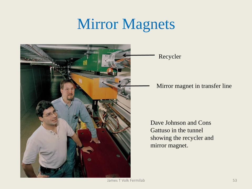
Mirror Magnets
James T Volk Fermilab 53
Dave Johnson and Cons
Gattuso in the tunnel
showing the recycler and
mirror magnet.
Recycler
Mirror magnet in transfer line

Sextupole
James T Volk Fermilab 54
There was a need to cancel the
sextupole moments of 4 recycler
gradient magnets. To do this 4
permanent magnet sextupoles
were built.
These were Halbach array style
magnets with the easy axis
alternating around a ring.
The gradients were between
300 and 400 Kilo-Gauss/m2
In the spaces between the magnets
washers were placed to tune the
harmonics

Construction of Sextupoles
James T Volk Fermilab 55
These magnets had to clamp
around the beam pipe could
not break vacuum. They were
built in two sections that
bolted together
There were Aluminum spacers
between each brick. The holes
held steel rods and washers to
allow for strength adjustments.

Measurements
James T Volk Fermilab 56
Sextupole on the test stand at
MTF.
Hall probe scan of sextupole

Problems with the Recycler
• Heater tape– Stainless steel tape was added to the outside of the beam pipe for bake out
– The µ of the tape changed as the tape work hardened
– This introduced a sextupole moment that was un accounted for
– The tape had to be removed and new tape installed
– Should have tested field with beam pipe installed
• Vacuum– Vacuum took a long time to get to 10-11 Torr range necessary for storage ring
• Instrumentation– Not enough BPM and loss monitors at the beginning to determine orbits correctly
James T Volk Fermilab 57

Mini Boone Beam Line
James T Volk Fermilab 58
This is an 8 GeV transfer line from
the booster to the Mini Boone
target. PM quads were used with
EM bends and trims

Adjustable Permanent Magnets
Quadrupoles• Developed for the Next Linear Collider
• Quadrupoles were needed between RF cavities for
focusing
• Also to be used for Beam Based Alignment (BBA)
• Aperture 12.7 mm
• Gradient on the order of 100 Tesla per meter
• Vary field by 20% for BBA
• Maintain center stability of field to within
1 micro meter
James T Volk Fermilab 59
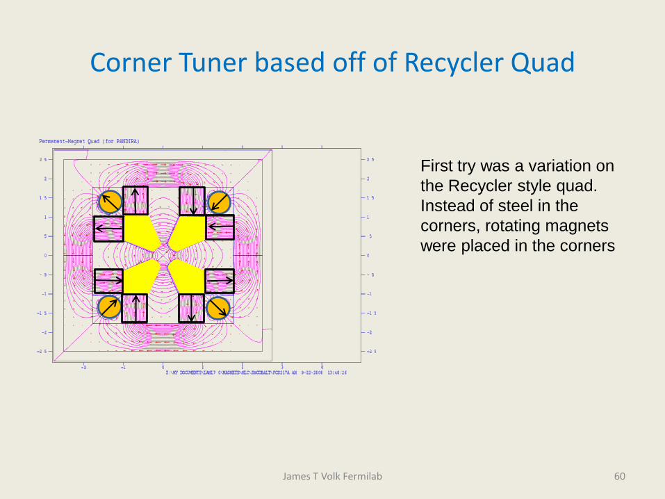
Corner Tuner based off of Recycler Quad
James T Volk Fermilab 60
First try was a variation on
the Recycler style quad.
Instead of steel in the
corners, rotating magnets
were placed in the corners

Corner Tuner based off of Recycler Quad
James T Volk Fermilab 61
First try was a variation on
the Recycler style quad.
Instead of steel in the
corners, rotating magnets
were placed in the corners

Center Stability of Corner Tuner
James T Volk Fermilab 62
Large variation of center
with angle of tuning rod
magnet was capable of
20% gradient change.

Wedge Quadrupole
Pole tips
Wedge magnets
Pole magnets
Tuning rods shown in max
field position
Flux returns
63James T Volk Fermilab

Wedge Quadrupole
Pole tips
Wedge magnets
Pole magnets
Tuning rods shown in max
field position
Flux returns
64James T Volk Fermilab

Wedge Quad Assembly and Test
James T Volk Fermilab 65
Side view of magnet showing tuning rod
Quad setup for stretched wire
measurements at MTF

Measuring Wedge Quad at SLAC
James T Volk Fermilab 66
End of Wedge quad
showing the rod turning
mechanism
Wedge quad on
rotating coils test
stand at SLAC

Center Stability of Wedge Quad
James T Volk Fermilab 67
Data taken at SLAC with
rotating coil
X center varies by 2
micro meters for 20%
change in gradient
Y center varies by 4
micro meters for a 20%
change in gradient
Magnets in rods not
totally balanced

Counter Rotating Quads
James T Volk Fermilab 68
Use fixed permanent
magnet quad and two
smaller rotating quads to
adjust the gradient

Counter Rotating Quadrupoles
James T Volk Fermilab 69
-0.005
-0.004
-0.003
-0.002
-0.001
0
0.001
0.002
0.003
-295
2
-317
0
-337
9
-354
6
-365
9
-355
5
-339
1
-318
6
-295
2
Integrated field gradient, T/m*cm
Xo
ffse
t, Y
off
set,
mm
Xoffset
Yoffset
Vladimir Kashikhin of Fermilab
developed a set of counter rotating
quadrupoles. The two inner quads
rotated on a stand relative to the outer
quads to vary the field.
The center stability was better
than 5 micro meters over the 20%
change in fields

Rotating Shunt Quadrupole
James T Volk Fermilab 70
Vladimir Kashikhin of Fermilab
developed a rotating shunt quad.
The permanent magnet material is in
red and the steel shunts are blue
The center stability less than 1 micron
See Magnet Technologies 17 for paper

Moving Magnetic Material to Change the Gradient
James T Volk Fermilab 71
Steve Gottschalk of STI Optronics
Seattle Washington developed an adjustable
quadrupole based on moving the magnetic material.
See PAC 2005 for paper
They were able to balance the different fields in
the magnet material by placement of the magnets.
The magnetic center stability is better than 0.5
micrometers over a 20% change

Center Line Shift
James T Volk Fermilab 72
Multiple passes varying strength
by 30% total shift less than 0.5
micro meters
Variation in strength for tuners
before and after adjustment of
position

Halbach Ring Quad
James T Volk Fermilab 73
Another type of adjustable quad,
the outer ring of magnets rotates to
change the field.
This was designed but the NLC was
canceled before it was built

Permanent Magnets and CLIC
James T Volk Fermilab 74
PARAMETER SCAN FOR THE CLIC DAMPING RINGSY. Papaphilippou, H.H. Braun, CERN, Geneva, Switzerland M. Korostelev Cockroft Institute, UK
EPAC 2008
Parameter Unit Symbol New value
2005
Old value
2007
beam energy [GeV] Eb 2.424 2.424
circumference [m] C 360 365.2
bunch population [109] N 110 312
bunch spacing [ns] Tsep 0.533 0.5
bunches per train Nb 110 312
number of trains Ntrain 4 1
store time / train [ms] tstore 13.3 20
rms bunch length [mm] σz 1.547 1.53
rms momentum spread [%] σδ 0.126 0.143
final hor. emittance [nm] γεx 550 381
hor. emittance w/o IBS
[nm]
γεx0 134 84
final vert. emittance [nm] γεy 3.3 4.1
coupling [%] κ 0.6 0.13
vertical dispersion
invariant
Hy 0 0.248
no. of arc bends nbend 96 100
arc-dipole field [T] Bbend 0.932 0.932
length of arc dipole [m] lbend 0.545 0.545
arc beam pipe radius [cm] barc 2 2
number of wigglers nw 76 76
wiggler field [T] Bw 1.7 2.5
length of wiggler [m] lw 2.0 2.0
wiggler period [cm] λw 10 5
wiggler half gap [cm] bw 0.6 0.5
mom. compaction [10−4] αc 0.796 0.804
synchrotron tune Qs 0.005 0.004
horizontal betatron tune Qx 69.82 69.84
vertical betatron tune Qy 34.86 33.80
RF frequency [GHz] fRF 1.875 2
energy loss / turn [MeV] U0 2.074 3.857
RF voltage [MV] VRF 2.39 4.115
h/v/l damping time [ms] τx/τy,/τs 2.8/2.8/1.4 1.5/1.5/0.76
revolution time [μs] Trev 1.2 1.2
repetition rate [Hz] frep 150 50

Permanent Magnets and CLIC
James T Volk Fermilab 75
PARAMETER SCAN FOR THE CLIC DAMPING RINGSY. Papaphilippou, H.H. Braun, CERN, Geneva, Switzerland M. Korostelev Cockroft Institute, UK
EPAC 2008
Parameter Unit Symbol New value
2005
Old value
2007
beam energy [GeV] Eb 2.424 2.424
circumference [m] C 360 365.2
bunch population [109] N 110 312
bunch spacing [ns] Tsep 0.533 0.5
bunches per train Nb 110 312
number of trains Ntrain 4 1
store time / train [ms] tstore 13.3 20
rms bunch length [mm] σz 1.547 1.53
rms momentum spread [%] σδ 0.126 0.143
final hor. emittance [nm] γεx 550 381
hor. emittance w/o IBS
[nm]
γεx0 134 84
final vert. emittance [nm] γεy 3.3 4.1
coupling [%] κ 0.6 0.13
vertical dispersion
invariant
Hy 0 0.248
no. of arc bends nbend 96 100
arc-dipole field [T] Bbend 0.932 0.932
length of arc dipole [m] lbend 0.545 0.545
arc beam pipe radius [cm] barc 2 2
number of wigglers nw 76 76
wiggler field [T] Bw 1.7 2.5
length of wiggler [m] lw 2.0 2.0
wiggler period [cm] λw 10 5
wiggler half gap [cm] bw 0.6 0.5
mom. compaction [10−4] αc 0.796 0.804
synchrotron tune Qs 0.005 0.004
horizontal betatron tune Qx 69.82 69.84
vertical betatron tune Qy 34.86 33.80
RF frequency [GHz] fRF 1.875 2
energy loss / turn [MeV] U0 2.074 3.857
RF voltage [MV] VRF 2.39 4.115
h/v/l damping time [ms] τx/τy,/τs 2.8/2.8/1.4 1.5/1.5/0.76
revolution time [μs] Trev 1.2 1.2
repetition rate [Hz] frep 150 50
0.932 Tesla bend field
2 cm pipe radius

23 mm Gap C Magnet
James T Volk Fermilab 76
23 mm gap
1.08 Tesla 13% higher
35 units of sextapole
20 units of decapole
These can be fixed with
pole shaping and end
shims
Poles
Magnet material samarium
Cobalt
Flux returns

From CLIC Nano Stablization pageThomas Zickler
Quadrupole Magnet
Nominal Gradient 200.1 T/m
Nominal integrated Gradient 370.0 T/m
Aperture radius 5.0 mm
Iron Length 1844.0 mm
Effective length 1849.0 mm
Total magnet weight 393.3 kG
Total magnet width 192.0 mm
Total magnet height 192.0 mm

From CLIC Nano Stablization pageThomas Zickler
Qaudrupole Magnet
Nominal Gradient 200.1 T/m
Nominal integrated Gradient 370.0 T/m
Aperture radius 5.0 mm
Iron Length 1844.0 mm
Effective length 1849.0 mm
Total magnet weight 393.3 kG
Total magnet width 192.0 mm
Total magnet height 192.0 mm

CLIC Quadrupole
James T Volk Fermilab 79
Nominal Gradient 200.1 Telsa/meter
Aperture radius 5 mm
Variation on Wedge quad
developed for NLC
208 Tesla/m gradient
Magnet material Ne-Fe-B magnets
Poles with 6.25 mm aperture radius
201.1 mm outside dimension

An Adjustable Quad
James T Volk Fermilab 80
Same as before
12.5 mm gap
Ne-Fe-B magnets
200 T/m tuners forward
180 T/m tuners reversed

Conclusions
• Permanent magnets are the solution for fixed energy beam lines and storage
rings
– Permanent magnets are stable in both time and temperature
– Permanent magnets are radiation hard
– For any fixed energy beam line or storage ring permanent magnets are the first choice;
the use of electromagnets must be justified!
– No power supplies or LCW -- this means no vibrations very important for storage and
damping rings
• Adjustable permanent quads can be made that are equal to if not better than
electro magnets
– Several different styles of adjustable quads were designed and built for the NLC
– Several met the spatial stability specifications
– One exceeded the spatial stability specifications
James T Volk Fermilab 81

Thank you
Questions?
James T Volk Fermilab 82