Periodic Relative Motion Near a

Keplerian Elliptic Orbit with

Nonlinear Differential Gravity∗

Prasenjit Sengupta†, Rajnish Sharma‡, and Srinivas R. Vadali§

Abstract

This paper presents a perturbation approach for determining relative motion initial condi-

tions for periodic motion in the vicinity of a Keplerian elliptic orbit of arbitrary eccentricity,

as well as an analytical solution for the relative orbit that accounts for quadratic nonlin-

earities in the differential gravitational acceleration. The analytical solution is obtained in

the phase space of the rotating coordinate system, centered at the reference satellite, and

is developed in terms of a small parameter relating relative orbit size, and semi-major axis

and eccentricity of the reference orbit. The results derived are applicable for arbitrary epoch

of the reference satellite. Relative orbits generated using the methodology of this paper

remain bounded over much longer periods in comparison to the results obtained using other

approximations found in the literature, since the semi-major axes of the satellites are shown

to be matched to the second order in the small parameter. The derived expressions thus

serve as excellent guesses for initiating a numerical procedure for matching the semi-major

axes of the two satellites. Several examples support the claims in this paper.

Introduction

Formation flying of spacecraft is an area of recent interest wherein the study of the

dynamics and control of relative motion is a key element. The applications of such formations

are varied, including terrestrial observation, communication, and stellar interferometry. Most

often, periodic or bounded relative orbits are desired for long-term formation maintenance,

during the periods when maneuvers are not called for. A set of benchmark problems for

spacecraft formation flying missions has been proposed by Carpenter et al.,1 that include

∗Presented as Paper AAS 06-162 at the 16th AAS/AIAA Spaceflight Mechanics Conference, Tampa, FL,January 2006.

†Ph.D. Candidate, Department of Aerospace Engineering, Texas A&M University, College Station,TX 77843-3141, prasenjit@tamu.edu, Student Member, AIAA.

‡Ph.D. Candidate, Department of Aerospace Engineering, Texas A&M University, College Station,TX 77843-3141, aeroraj@tamu.edu, Student Member, AIAA.

§Stewart & Stevenson-I Professor, Department of Aerospace Engineering, Texas A&M University, CollegeStation, TX 77843-3141, svadali@aero.tamu.edu, Associate Fellow, AIAA.

1 of 35

reference low Earth orbit (LEO) and highly elliptical orbit (HEO) missions. An example of

the latter is the Magnetosphere Multiscale Mission (MMS),2 where the apogee and perigee

are of the order of 12-30Re and 1.2Re, respectively (with Re denoting the radius of the

Earth), yielding eccentricities of the order of 0.8 and higher. The theoretical development

in this paper primarily concentrate on cases where the reference orbit has high eccentricity,

while treating LEO missions as a special case.

The most common model describing relative motion near a Keplerian orbit is given by the

Hill-Clohessy-Wiltshire (HCW) equations.3 This model assumes a circular reference orbit

and linearized differential gravity model, based on the two-body problem. Conditions for

bounded motion, designated as HCW initial conditions, can be easily derived for this model

and they have found wide applicability for formation flight. Though the relative motion

between two spacecraft in Keplerian orbits is always bounded, for the purpose of formation

flight, the term “bounded”, as in this paper, refers to 1:1 resonance where the periods of all

spacecraft are the same. The applicability of the HCW conditions is limited when any of

the underlying assumptions are violated, viz. eccentric reference orbit, nonlinear differential

gravity, aspherical Earth, and other perturbations. Since these factors accurately represent

the realities of any mission, modifications to the model must be made to account for, and

negate if possible, these effects. Previous work, limiting attention only to the two-body

problem, may be categorized into those that deal with 1) nonlinear differential gravity, 2)

noncircular reference orbit, and 3) the combination of nonlinearity and noncircular orbits.

References 4–6 treated second-order nonlinearities as perturbations to the HCW equations

and found approximate solutions to the system. Reference 7 also included the solution

to the third-order perturbed equation, with periodicity conditions enforced on the linear

equation. The eccentricity problem has been treated by using either time or true anomaly as

the independent variable. The linear problem for eccentric reference orbits was introduced

by Tschauner and Hempel.8 de Vries9 obtained analytical expressions for relative motion

using the Tschauner-Hempel (TH) equations, accurate to first order in eccentricity. Kolemen

and Kasdin10 also obtained a closed-form solution to periodic relative motion by treating

eccentricity as a perturbation to a Hamiltonian formulation of the linearized HCW equations.

The TH equations admit solutions in the form of special integrals, which have been derived in

Refs. 11–13. These solutions have been used to obtain state transition matrices for relative

motion near an orbit of arbitrary eccentricity14,15 using true anomaly as the independent

variable, assuming a linearized differential gravity field. State transition matrices for relative

motion using time as the independent variable have also been developed by Melton16 and

Broucke.17 Reference 16 used a series expansion for radial distance and true anomaly, in

terms of time. However, for moderate eccentricities, the convergence of such series requires

2 of 35

the inclusion of many higher-order terms. Inalhan et al.,18 utilizing Carter’s work in Ref. 13,

developed the conditions under which the TH equations admit periodic solutions.

Literature on establishing initial conditions for formations amply shows the importance

of addressing the effects of eccentricity as well as nonlinearity. To this end, Anthony and

Sasaki19 obtained approximate solutions to the HCW equations by including quadratic non-

linearities and first-order eccentricity effects. Vaddi et al.20 studied the combined problem

of eccentricity and nonlinearity and obtained periodicity conditions in the presence of these

effects. However, these conditions lose validity even for intermediate eccentricities, primarily

because of the higher-order coupling between eccentricity and nonlinearity. Recent work by

Gurfil21 poses the bounded-motion problem in terms of the energy-matching condition. Since

the velocity appears in a quadratic fashion in this equation, velocity corrections to the full,

nonlinear problem can be obtained in an analytical manner, without assumptions on relative

orbit size. However, the more general problem of period-matching is reduced to the solution

of a sixth-order algebraic equation in any of the states, assuming the other five states are

known. This approach requires a numerical procedure to obtain a solution, starting with an

initial guess. The sixth-order polynomial has multiple roots, some of which have no physical

significance. Euler and Schulman22 first presented the TH equations perturbed by nonlinear

differential gravity with no assumptions on eccentricity. However, they claimed that these

equations could not be solved analytically.

Relative motion can also be characterized in a linear setting, by the use of differential

orbital elements.23–28 Due to the nonlinear mapping between local frame Cartesian coordi-

nates and orbital elements, errors in the Cartesian frame are translated into very small errors

in the orbital angles. References 23–25 approached the problem by linearizing the direction

cosine matrix of the orientation of the Deputy with respect to the Chief. Reference 26 used

true anomaly as the independent variable to obtain analytical expressions for relative motion

near high-eccentricity orbits. The same objective was achieved by Sabol et al.,27 but in a

time-explicit manner. In this case, a Fourier-Bessel expansion of the true anomaly in terms

of the mean anomaly was used. However, for eccentricities of 0.7, terms up to the tenth order

in eccentricity are required in the series. In Ref. 28, a methodology has been proposed where

Kepler’s equation29 is solved for the Deputy, but is not required for the Chief, if the Chief’s

true anomaly is used as the independent variable. While Refs. 26–28 provide accurate results

for highly eccentric reference orbits, only Ref. 23–25 allow characterizing such orbital ele-

ment differences in terms of the constants of the HCW solutions, viz. relative orbit size and

phase. The basic zero-secular drift condition is satisfied by setting the semi-major axis of the

Deputy and Chief to be the same. The characterization of relative orbit geometry is achieved

by relating the rest of the orbital element differences to its shape, size, and the initial phase

3 of 35

angle. Alfriend et al.30 also introduced nonlinearities in the orbital element approach by

using quadratic differential orbital elements in the geometric description of formation flight.

Though much work has been done on the problem of formation flight using orbital ele-

ments, in many ways, the use of relative motion equations in the local (rotating) Cartesian

frame is preferred over orbital element differences. It is easier to obtain local ranging data

directly, than to have the position and velocity of either satellite reported to a terrestrial

station and translated into orbital elements. This also allows the use of decentralized con-

trol algorithms for the control of formations. Furthermore, the geometry specification in

the orbital element approach followed in Refs. 23–25 assumes truncation of the eccentricity

expansion to first order. For moderate or high eccentricities, this may lead to relative orbit

geometry that is different from what is desired.

The work in this paper studies the perturbed TH equations by treating second-order

nonlinearities. In effect, the problem posed in Ref. 22 is solved. These results are valid

for arbitrary eccentricities and implicitly account for eccentricity-nonlinearity effects. The

exact analytical solution, while complicated in appearance at first, leads to an elegant form

of expressions for relative motion. Furthermore, the terms that lead to secular growth in

the perturbed equations are easily identified as those that also lead to secular growth in

the unperturbed equation, as observed in Ref. 13. Consequently, collecting these terms and

negating their effects leads to a valid condition for periodic orbits. It should be noted that

this paper assumes a central gravity field without the effect of perturbations such as drag

and J2. A description of the relative motion problem in the presence of these perturbations

may be found in Ref. 31.

Problem Description

Reference Frames

Consider an Earth-centerd inertial (ECI) frame, denoted by N , with orthonormal basis

BN = {ix iy iz}. The vectors ix and iy lie in the equatorial plane, with ix coinciding

with the line of the equinoxes, and iz passes through the North Pole. The analysis uses

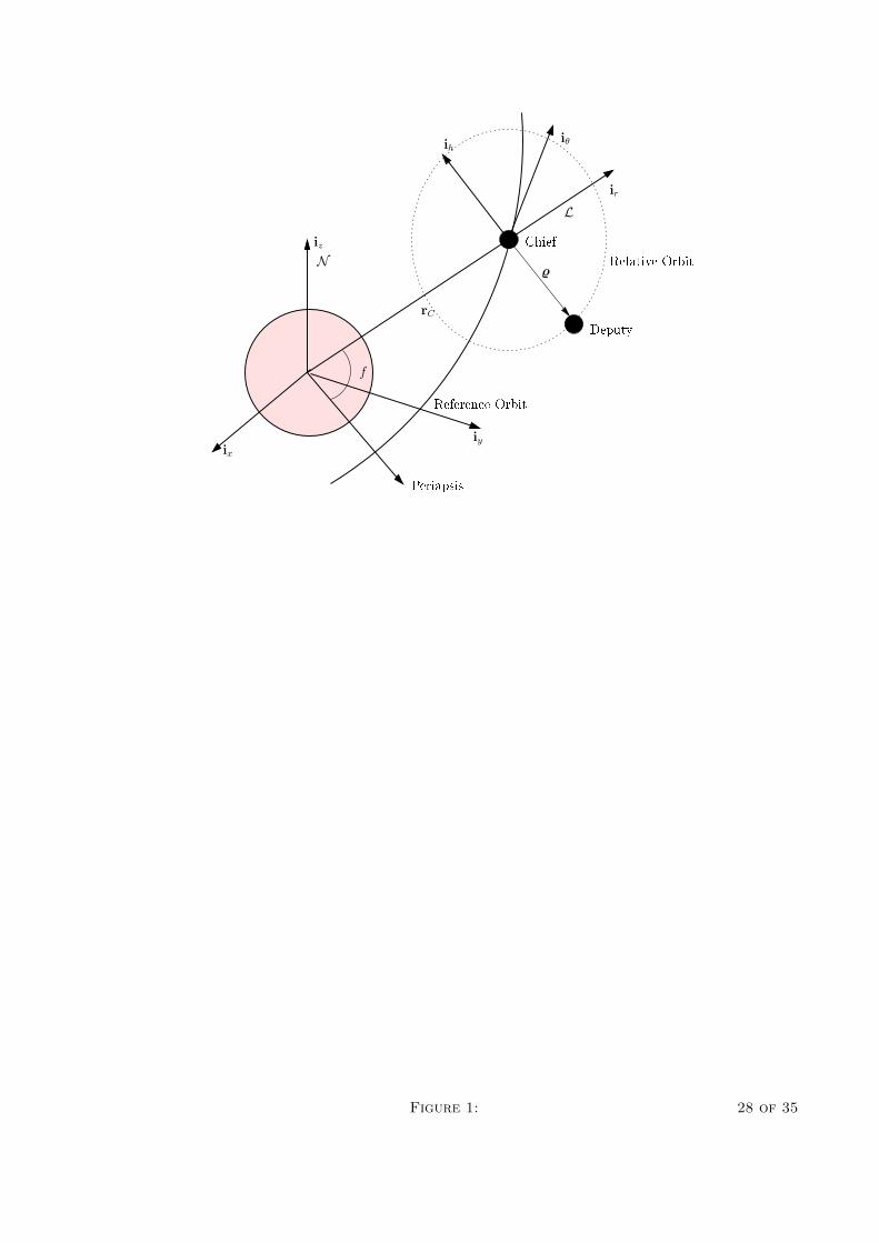
a Local-Vertical-Local-Horizontal (LVLH) frame, as shown in Fig. 1 and denoted by L,

that is attached to the target satellite (also called Leader or Chief). This frame has basis

BL = {ir iθ ih}, with ir lying along the radius vector from the Earth’s center to the

satellite, ih coinciding with the normal vector to the plane defined by the position and

velocity vectors of the satellite, and iθ = ih × ir. In this frame, the position of the Chief is

denoted by rC = rir, where r is the radial distance, and the position of the chaser satellite

(also known as the Follower or Deputy) is denoted by rD = rC + % where % = ξir + ηiθ + ζih

is the position of the Deputy relative to the Chief.

4 of 35

Equations of Motion

The equations of motion may be derived using a Lagrangian formulation, which requires

the gravitational potential of the Deputy:

V = − µ

|rD| = −µ

r

(1 +

%2

r2+ 2

ξ

r

)− 12

(1)

Observing that ξ/r = (ξ/%) · (%/r), the parenthesised term in the above equation is then the

generating function for Legendre polynomials with argument −ξ/%. Consequently,

V = −µ

r

∞∑

k=0

(−1)k(%

r

)k

Pk(ξ/%) = −µ

r

[1− ξ

r+

1

2

(2ξ2 − η2 − ζ2)

r2

]+ V (2)

V = −µ

r

∞∑

k=3

(−1)k(%

r

)k

Pk(ξ/%) (3)

where Pk is the kth Legendre polynomial. Consequently, the equations of motion are:

ξ − 2θη −(θ2 + 2

µ

r3

)ξ − θη = −∂V

∂ξ(4a)

η + 2θξ −(θ2 − µ

r3

)η + θξ = −∂V

∂η(4b)

ζ +µ

r3ζ = −∂V

∂ζ(4c)

where θ is the argument of latitude given by θ = ω + f , with ω denoting the argument

of periapsis and f , the true anomaly. Also useful are the equations for the radius and the

argument of latitude:29

r = θ2r − µ

r2(5a)

θ = −2r

rθ (5b)

Higher-order Legendre polynomials in the perturbing potential can be generated from lower-

order ones, by using the recursive relation (k + 1)Pk+1(z) = (2k + 1)zPk(z) − kPk−1(z),

with P0(z) = 1 and P1(z) = z. The perturbing gravitational acceleration ∂V /∂% =

{∂V /∂ξ ∂V /∂η ∂V /∂ζ}T contributes higher-order nonlinearities to the system, and if

ignored, allows the treatment of Eq. (4) as a tenth-order linear system (additional equa-

tions are contributed by Keplerian motion). This can be converted to a sixth-order linear

system with periodic coefficients, if the independent variable is changed from t to f . Use

5 of 35

is made of the formulae f = h/r2 where the angular momentum h =√

µa(1− e2) and

r = a(1− e2)/(1 + e cos f), with semi-major axis a and eccentricity e. Consequently,

( ˙ ) = f( ′ ) = n(1 + e cos f)2( ′ ) (6a)

(¨) = f 2( ′′ ) + f( ′ )

= n2(1 + e cos f)3[(1 + e cos f)( ′′ )− 2e sin f( ′ )

](6b)

where ( ′ ) denotes the derivative with respect to f , n = n/(1− e2)3/2, and n =√

(µ/a3) is

the mean motion.

To calculate the perturbing differential gravitational acceleration ∂V /∂%, the following

relation is made use of:

d

dzPk(z) =

k

z2 − 1[zPk(z)− Pk−1(z)] (7)

Using %2 = ξ2 + η2 + ζ2, and ∂ξ/∂% = ir, it can be shown that:

∂V

∂%= − µ

r3

∞∑

k=3

(−1)k(%

r

)k−2 k

η2 + ζ2

[%2Pk(ξ/%)i1 + %Pk−1(ξ/%)i2

](8)

where i1 = ηiθ +ζih and i2 = (η2 +ζ2)ir−ξηiθ−ξζih. Upon resolution, the perturbing differ-

ential gravity field can be rewritten as a series involving the following small, dimensionless

parameter:

ε =%0

a(1− e2)(9)

where, %0 is some measure of the relative orbit size. For low eccentricities, this may be

the circular orbit radius as predicted by the HCW solutions. Without loss of generality,

%0 =√

(ξ20 + η2

0 + ζ20 ) ¿ a. The expression for the perturbed gravitational acceleration,

along with Eq. (6) is now used in Eq. (4). Furthermore, the system of equations is divided

by n2(1 + e cos f)4 that appears on both sides of the equation. A nondimensional position

vector ρ = xir+yiθ+zih is introduced. This vector is obtained from % by nondimensionalizing

it with respect to %0, and by the following transformation:8,12

ρ =%

%0

(1 + e cos f) (10)

6 of 35

Consequently,

ρ′ =%′

%0

(1 + e cos f)− %

%0

e sin f (11a)

ρ′′ =%′′

%0

(1 + e cos f)− 2%′

%0

e sin f − %

%0

e cos f (11b)

The complete equations of motion are as follows:

x′′

y′′

z′′

+

0 −2 0

2 0 0

0 0 0

x′

y′

z′

+

−3/(1 + e cos f) 0 0

0 0 0

0 0 1

x

y

z

=∞∑

k=3

εk−2(−1)kk

(1 + e cos f)(y2 + z2)

ρkPk(x/ρ)

0

y

z

+ ρk−1Pk−1(x/ρ)

y2 + z2

−xy

−xz

= ε3

2(1 + e cos f)−1

y2 + z2 − 2x2

2xy

2xz

+O(ε2) (12)

From Eq. (12), it is evident that if the terms of order ε and higher are ignored, then the

equations reduce to the unperturbed Tschauner-Hempel equations. Additionally, if e = 0,

then the HCW equations are obtained. It should be noted that the small parameter ε depends

not only on the size of the relative orbit, but also on the eccentricity of the reference. This

reflects the fact that eccentricity and nonlinearity effects in formation flight are coupled.

Solution Using a Perturbation Approach

A straightforward expansion32 of the following form is considered:

x(f) = x0(f) + εx1(f) + · · ·y(f) = y0(f) + εy1(f) + · · · (13)

z(f) = z0(f) + εz1(f) + · · ·

Lindstedt-Poincare or renormalization techniques are not required since a frequency correc-

tion is not necessary: In a central gravity field, periodic motion between two satellites is only

possible when the two satellites have the same mean motion. Consequently, the frequency

of the relative orbit is the same as that of the orbits of either satellite. It will be shown

that the most general solution for bounded orbits of the TH equations, without perturba-

tions (zeroth-order equations), has the same frequency as the orbital period of each satellite.

7 of 35

Consequently, higher-order corrections to the frequency must necessarily be zero, since the

coefficient corresponding to each correction is an increasing power of the small parameter.

Equation (13) is substituted in Eq. (12), with perturbations up to order ε included.

Collecting terms of the same order, the following two systems are obtained:

x′′0 − 2y′0 −3x0

(1 + e cos f)= 0 (14a)

y′′0 + 2x′0 = 0 (14b)

z′′0 + z0 = 0 (14c)

and,

x′′1 − 2y′1 −3x1

(1 + e cos f)=

3

2

(y20 + z2

0 − 2x20)

(1 + e cos f)(15a)

y′′1 + 2x′1 =3x0y0

(1 + e cos f)(15b)

z′′1 + z1 =3x0z0

(1 + e cos f)(15c)

Solution to the Unperturbed System

The approach followed in this section is for epoch at a general initial value of true anomaly

fi. In a later section, the explicit formulation for fi = 0 (periapsis) and fi = π (apoapsis)

will be presented. This considerably simplifies the expressions obtained.

It can be shown that the solution to the homogeneous zeroth-order system given by

Eqs. (14) is:12,13

x0(f) = c1 cos f (1 + e cos f) + c2 sin f (1 + e cos f)

+c3

[2e sin f (1 + e cos f)H(f)− cos f

(1 + e cos f)

](16a)

y0(f) = −c1 sin f (2 + e cos f) + c2 cos f (2 + e cos f)

+2c3(1 + e cos f)2H(f) + c4 (16b)

z0(f) = c5 cos f + c6 sin f (16c)

x′0(f) = −c1(sin f + e sin 2f) + c2(cos f + e cos 2f)

+c3

[2e(cos f + e cos 2f)H(f) +

(sin f + e sin 2f)

(1 + e cos f)2

](16d)

y′0(f) = −c1(2 cos f + e cos 2f)− c2(2 sin f + e sin 2f)

−2c3

[e(2 sin f + e sin 2f)H(f)− cos f

(1 + e cos f)

](16e)

z′0(f) = −c5 sin f + c6 cos f (16f)

8 of 35

where H(f) is a function evaluated in terms of the eccentric anomaly, E:13

H(f) =

∫cos f

(1 + e cos f)3df

= −(1− e2)−5/2

[3e

2E − (1 + e2) sin E +

e

4sin 2E

](17)

The following equations relate the eccentric and true anomalies:29

cos f =cos E − e

1− e cos E, sin f =

(1− e2)1/2 sin E

1− e cos E

cos E =cos f + e

1 + e cos f, sin E =

(1− e2)1/2 sin f

1 + e cos f

It is shown in Ref. 33 that a first-order periodicity condition can easily be derived by

studying Eqs. (16). Let the initial conditions for the zeroth-order (unperturbed) system

be denoted by the vector x0i= {x0i

y0iz0i

x′0iy′0i

z′0i}T , specified at arbitrary initial true

anomaly fi, and let the vector of integration constants be denoted by c = {c1 · · · c6}T , the

relation x0i= Lc holds. The entries of matrix L, denoted by Ljk, j = 0 . . . 6, k = 0 . . . 6,

are constructed by substituting fi in the right hand side of Eq. (16). From the structure of

Eq. (16) and Eq. (17), it is observed that secular growth is contributed by those terms with

coefficient c3. This is also observed in Ref. 18. Consequently, the generalized condition for

periodicity33 is:

l1x0i+ l2x

′0i

+ l3y′0i

= 0 (18)

where, l1 = L52L41 − L51L42 = e2 + 3e cos fi + 2

l2 = L12L51 − L11L52 = e sin fi(1 + e cos fi)

l3 = L42L11 − L41L12 = (1 + e cos fi)2

This condition is satisfied for infinite combinations of initial conditions, and for resolution,

a constraint is required. One suitable constraint may be to keep the initial states as a given

and calculate the minimum velocity impulse required to obtain a periodic orbit. A similar

approach has been used in Ref. 18, wherein the ∆v for formation insertion is minimized by

posing the problem as a linear program. The problem may also be posed as one where the

2-norm of the impulse, with components ∆x′0 and ∆y′0, is minimized:

min Φ(∆x′0, ∆y′0) =(

∆x′20 + ∆y′20)1/2

subject to : Ψ(∆x′0, ∆y′0) = l1x0i+ l2

(x′0i

+ ∆x′0)

+ l3(y′0i

+ ∆y′0)

= 0 (19)

9 of 35

By minimizing Φ + λΨ, where λ is a Lagrange multiplier, the following unique solution is

obtained:

∆x′0 = − l2l22 + l23

(l1x0i+ l2x

′0i

+ l3y′0i

) (20a)

∆y′0 = − l3l22 + l23

(l1x0i+ l2x

′0i

+ l3y′0i

) (20b)

Irrespective of the manner in which the initial conditions are established, as long as c3 = 0,

the most general periodic solution to the TH equations may be rewritten as:33

xp(f) = ρ1 sin(f + α) (1 + e cos f) (21a)

yp(f) = ρ1 cos(f + α) (2 + e cos f) + ρ2 (21b)

zp(f) = ρ3 sin(f + β) (21c)

where the subscript ‘p’ denotes a periodic relative orbit. The relative orbit parameters ρ1

and ρ3 indicate relative orbit size, ρ2 introduces a bias in along-track motion, and the angles

α and β indicate the phase of the Deputy. These relative orbit parameters may be obtained

from the integration constants, by the following:

ρ1 =(c21 + c2

2

)1/2, ρ2 = c4, ρ3 =

(c25 + c2

6

)1/2(22a)

α = tan−1

(c1

c2

), β = tan−1

(c5

c6

)(22b)

If e = 0, then the solutions are the same as those for the HCW equations. It is now evident

that circular orbits in the fashion of HCW projected circular orbit or general circular orbit,

cannot be obtained if e 6= 0.

Solution to the Perturbed System

Having obtained initial conditions for periodicity in the unperturbed system, its periodic

form is now substituted in Eqs. (15). The solutions to these equations are similar to Eqs. (16),

with additional particular integrals. The equation in z1(f) is considered separately, due to

its tractable nature:

z′′1 + z1 =3xpzp

(1 + e cos f)= 3ρ1ρ3 sin(f + α) sin(f + β) (23)

Solving Eq. (23) yields:

z1(f) = k1 cos f + k2 sin f +1

2ρ1ρ3 [3 cos(α− β) + cos(2f + α + β)] (24)

10 of 35

Since there are no secular growth terms in Eq. (24), an arbitrary choice may be made for the

constants of integration k1 and k2. To remove terms with cos(f) and sin(f), i.e., to ensure

that the mean value of the z amplitude is the same as that predicted by the linear equations,

the following choices for the initial conditions are made:

z1i=

1

2ρ1ρ3 cos(2fi + α + β) +

3

2ρ1ρ3 cos(α− β) (25a)

z′1i= −ρ1ρ3 sin(2fi + α + β) (25b)

As a result,

z1(f) =3

2ρ1ρ3 cos(α− β) +

1

2ρ1ρ3 cos(2f + α + β) (26)

Reference 12 develops the TH equations in the presence of a forcing function. Utilizing

this result, it can be shown that the x1 and y1 solutions are:

x1(f) = b1 cos f (1 + e cos f) + b2 sin f (1 + e cos f) (27a)

+b3

[2e sin f (1 + e cos f)H(f)− cos f

(1 + e cos f)

]+ φ

∫L

φ2df

y1(f) = −b1 sin f (2 + e cos f) + b2 cos f (2 + e cos f) (27b)

+2b3(1 + e cos f)2H(f) + b4 + 3

∫∫xpyp

(1 + e cos f)df

+1

e

[(1 + e cos f)2

∫L

φ2df −

∫L

sin2 fdf

]

where φ = sin f (1 + e cos f), and

L =3

2

∫(y2

p + z2p − 2x2

p) sin f df − 3

e(1 + e cos f)2

∫xpyp

(1 + e cos f)df

+3

e

∫xpyp(1 + e cos f) df

= L0 +5∑

k=1

(Lckcos kf + Lsk

sin kf) (28)

The coefficients, {L0, Lc1 · · ·Lc5 , Ls1 · · ·Ls5} are provided in the appendix. The complete

solution of Eqs. (27) requires the evaluation of the integrals of cos(kf)/φ2, sin(kf)/φ2,

cos(kf)/ sin2 f , and sin(kf)/ sin2 f , k = 1 . . . 5. These integrals can also be evaluated in

terms of H(f) and sinusoidal functions of the true anomaly, and are presented in the ap-

pendix. Though it may appear that the terms in the appendix are not defined for f = nπ, it

should be noted that when multiplied by the appropriate coefficient, the logarithmic terms,

11 of 35

and terms containing f explicitly, cancel each other, and are therefore ignored from further

analysis. Consequently, the analytical solution to the perturbed system can be constructed.

From the appendix and the solution to Eq. (27a), the secular growth terms are identified

as those which contain H(f). It follows that setting the combined coefficient of H(f) to zero

will prevent secular growth to the second order. Collecting the coefficients of H(f) in x1(f)

results in the following condition:

2eb3 + 2eL0 − 2

3(2 + e2)Lc1 +

2

3e(2 + e2)Lc2 − 2(2− e2)Lc3

− 2

3e3(8− 24e2 + 13e4)Lc4 −

2

3e4(32− 80e2 + 50e4 − 5e6)Lc5 = 0 (29)

or b3 = −e

4

(2ρ2

1 cos 2α + ρ23 cos 2β

)− 2ρ1ρ2 cos α− e

4

(ρ2

1 + 2ρ22 + ρ2

3

)

− 1

2e

(2ρ2

1 + 2ρ22 + ρ2

3

)(30)

The seemingly complex integrals involved in the equation actually reduce to fairly simple

expressions. Ignoring the terms containing H(f), since they are rendered absent by the

choice of b3 in Eq. (30), the integrals may be rewritten as the following:

p1(f) = φ

∫L

φ2df =

3∑

k=1

Gk sin kf +1

(1 + e cos f)

4∑

k=0

Hk cos kf (31a)

q1(f) = 3

∫∫xpyp

(1 + e cos f)df =

3∑

k=1

(Ek sin kf + Fk cos kf) (31b)

q2(f) =1

e

[(1 + e cos f)2

∫L

φ2df −

∫L

sin2 fdf

]

= D0 +3∑

k=1

(Ck sin kf + Dk cos kf) (31c)

The coefficients are presented in the appendix.

The initial conditions for the perturbed system, x1i= {x1i

y1ix′1i

y′1i}T , integration

constants b = {b1 · · · b4}T , and initial values of the forcing function, are related by the

following:

x1i= Lb + w (32)

12 of 35

It follows that:

L =

L11 L12 L13 0

L21 L22 L23 1

L41 L42 L43 0

L51 L52 L53 0

(33)

It is shown in Ref. 33 that detL = L13l1 + L43l2 + L53l3 = 1. The initial values of the forcing

functions are given by w = {p1 (q1 + q2) p′1 (−2p1 + q′1)}T evaluated at f = fi.

Initial conditions are required that will lead to the particular value of b3 specified in

Eq. (30). This provides one constraint on the initial conditions. If only a velocity correction

is required, one may choose x1i= y1i

= x′1i= 0. By substituting the b1...3 obtained from

solving Eq. (32) into the last equation for y′1i, the following is obtained:

y′1i=

l1l3

(p1 + L13b3) +l2l3

(p′1 + L43b3) + L53b3 − 2p1 + q′1

= −e(cos fi + e cos 2fi)

(1 + e cos fi)2p1 +

e sin fi

(1 + e cos fi)p′1 + q′1 +

eb3

(1 + e cos fi)2= ∆ (34)

It should be noted that the apparent zero-eccentricity singularity in Eq. (30) is removed by

the e multiplier in Eq. (34). The quantity ∆ specifies the correction to the initial conditions

required to negate secular growth arising from second-order differential gravity. Conse-

quently,

∆x′ = − l2l22 + l23

[l1x(fi) + l2x′(fi) + l3y

′(fi)] (35a)

∆y′ = − l3l22 + l23

[l1x(fi) + l2x′(fi) + l3y

′(fi)] + ε∆ (35b)

To convert this to initial relative position and velocity,(ξi, ηi, ζi, ξi, ηi, ζi

)with time as

the independent variable, the following transformation may be used:

ξi

ηi

ζi

=%0

(1 + e cos fi)

xi

yi

zi

(36a)

ξi

ηi

ζi

= %0n(1 + e cos fi)

x′iy′iz′i

+ %0ne sin fi

xi

yi

zi

(36b)

13 of 35

Time itself can be obtained from the direct solution to Kepler’s equation:

t =1

n(E − e sin E) (37)

Epoch at Periapsis/Apoapsis

The expressions are simplified greatly if it is assumed that fi = 0 or fi = π. At these

values of fi, l2 = 0. The condition for periodicity in the linearized field reduces to:

y′0i= −(2± e)

(1± e)x0i

(38)

where the positive and negative signs denote fi = 0 and fi = π, respectively. These are

obtained in an equivalent fashion in Ref. 18. Since l2 = 0, it is now unnecessary to evaluate

p′1. From the expressions for L0, Lckand Lsk

that are presented in the appendix, it is

observed that:

p1(0) = − 1

(1 + e)

(L0 +

5∑

k=1

Lck

)(39a)

=1

(1 + e)

[1

4ρ3

2 cos 2 β − 1

4ρ1

2(5 e + e2 + 2

)cos 2 α

−ρ1ρ2 (3 + e) cos α +3

2ρ1

2 − 1

4ρ1

2e2 +3

4ρ3

2 +3

2ρ2

2

]

p1(π) =1

(1− e)

(L0 +

5∑

k=1

(−1)kLck

)(39b)

=1

(1− e)

[1

4ρ3

2 cos 2 β − 1

4ρ1

2(−5 e + e2 + 2

)cos 2 α

+ρ1ρ2 (3− e) cos α +3

2ρ1

2 − 1

4ρ1

2e2 +3

4ρ3

2 +3

2ρ2

2

]

By substituting p1, q′1 = E1 + 2E2 + 3E3 and b3 in Eq. (34), the initial condition correction

is:

y′1i=

1

4

(e2 ∓ 2 e− 4) ρ12

1± e− 1

4

(2± e)

(1± e)

(2ρ2

2 + ρ23

)∓ 1

4

eρ32 cos 2 β

1± e

−1

4

ρ12 (3 e2 ± 8 e + 6) cos 2 α

1± e− ρ1ρ2 (2 e± 3) cos α

1± e(40)

Second-Order Analytical Expressions for Relative Motion

Since the the choice of the constants b1, b2, and b4 is arbitrary, they may be chosen to yield

a suitable second-order equation for relative motion. Equation (27b) is now reconsidered.

14 of 35

Upon substituting Eq. (30) in Eq. (27b), it can be shown that:

y1(f) = (−2b1 + C1 + E1) sin f +

(−eb1

2+ C2 + E2

)sin 2f + (C3 + E3) sin 3f

+ (2b2 + D1 + F1) cos f +

(eb2

2+ D2 + F2

)cos 2f + (D3 + F3) cos 3f

+

(eb2

2+ b4 + D0

)(41)

It is observed that C3 = −E3 and D3 = −F3. The values of b1, b2, and b4 can be chosen

such that the coefficients of sin f and cos f , and the constant term are zero. In this event,

b1 =1

2(C1 + E1) (42a)

b2 = −1

2(D1 + F1) (42b)

b4 = −D0 − eb2

2(42c)

Consequently,

y1(f) =

(−eC1

4− eE1

4+ C2 + E2

)sin 2f +

(−eD1

4− eF1

4+ D2 + F2

)cos 2f

= −e2

8ρ2

1 sin 2f +e

4ρ1ρ2 sin(2f + α)− 1

8(2− e2)ρ2

1 sin(2f + 2α)

−1

4ρ2

3 sin(2f + 2β) (43)

Now, Eq. (27a) is considered, after the removal of secular terms. In this case,

x1(f) = b1 cos f (1 + e cos f) + b2 sin f (1 + e cos f) + G1 sin f + G2 sin 2f + G3 sin 3f

+1

(1 + e cos f)[H0 + (H1 − b3) cos f + H2 cos 2f + H3 cos 3f + H4 cos 4f ] (44)

It can be shown that

1

(1 + e cos f)[H0 + (H1 − b3) cos f + H2 cos 2f + H3 cos 3f + H4 cos 4f ]

= N1 cos f + N2 cos 2f + N3 cos 3f (45)

where N1 = −C1/2, N2 = −C2, and N3 = −3C3/2. It follows that:

x1(f) =eb1

2+ (b1 + N1) cos f + (b2 + G1) sin f +

(eb1

2+ N2

)cos 2f

15 of 35

+

(eb2

2+ G2

)sin 2f + N3 cos 3f + G3 cos 3f

= −1

8

[(4− e2

)ρ2

1 + 4ρ22 + 2ρ2

3

]− e

4ρ1ρ2 cos α− e2

8ρ2

1 cos 2α

−3

2ρ1ρ2 cos(f + α)− 3e

8ρ2

1 cos(f + 2α)− e

4ρ1 ρ2 cos (2f + α)

+e2

8ρ1

2 cos 2f − 1

8(4 + e2) ρ1

2 cos (2f + 2α) +1

4ρ3

2 cos (2f + 2β)

−e

8ρ2

1 cos(3f + 2α) (46)

The analytical solution for a relative orbit near a Keplerian orbit, accounting for second-

order terms, is thus given by Eqs. (13), with x0(f), y0(f), and z0(f) given by Eqs. (21), and

x1(f), y1(f), and z1(f) by Eq. (46), Eq. (43), and Eq. (24), respectively.

Periodic Orbits and the Energy-Matching Condition

Two spacecraft in Keplerian elliptic orbits will have periodic relative motion if the total

energy E of each spacecraft (and consequently, the semi-major axis of each spacecraft) is the

same. Denoting the quantities of the Deputy with subscript ‘D’ and those of the Chief with

subscript ‘C’, the vis-viva equation29 for each spacecraft leads to the following condition for

periodic relative motion:

∆E(ξ, η, ζ, ξ, η, ζ) , ED − EC = −(

µ

2aD

− µ

2ac

)=

(v2

D

2− µ

rD

)−

(v2

C

2− µ

rC

)= 0 (47)

Using rD = (r + ξ)ir + ηiθ + ζih, and vD = (r + ξ − θη)ir + (η + θξ + θr)iθ + ζih, and

normalizing these quantities in the same manner as that in the previous sections, Eq. (47)

can be rewritten as:

∆E(ρ,ρ′) =(2 + 3ecf + e2)

(1 + ecf )x + esfx

′ + (1 + ecf )y′

+ε

2(1 + ecf )

[− (1− e2)x2 + (2 + 3ecf + e2)y2 + (1 + ecf + e2s2

f )z2

+(1 + ecf )2(x′2 + y′2 + z′2) + 2esf (1 + ecf )(xx′ + yy′ + zz′)

+2(1 + ecf )2(xy′ − yx′)

]+

∞∑n=2

(−1)nεnρn+1Pn+1

(x

ρ

)= 0 (48)

where cf and sf denote the cosine and sine of f , respectively. If terms of O(ε) and higher are

neglected, then Eq. (48) is exactly the same as Eq. (18). Appending the correction scheme

developed in this paper, to the initial conditions leads to ∆E(ρ,ρ′) = O(ε2). This may be

16 of 35

observed by using Eq. (40), and setting f = 0 in Eq. (48). Consequently,

∆E ≈ µ

2a2∆a ≈ %0a(1− e2)n2ε2 (49a)

∆a =2%3

0

a2(1− e2)4(49b)

The effect of eccentricity on the semi-major axis difference is thus clearly evident.

The formation-keeping problem may be posed by appending ∆E(ρ,ρ′) = 0 as a constraint

to a cost function comprising velocity increments. In Ref. 21 it is shown that instead of

expanding the period-matching condition in terms of Legendre polynomials, the velocity

increments can be solved for the complete nonlinear system analytically. This is possible

because the relative velocity terms appear only up to the second order in Eq. (48).

Drift Measurement

To measure the efficacy of the initial condition corrections developed in this paper, an

index is desired that captures secular drift and periodic motion behavior. Unlike the solutions

to the linear, autonomous HCW equations, circular relative orbits in the general elliptic case

cannot be obtained. Consequently, a new measure of deviation from the nominal solution is

desired, which can be used to compare the results in this paper, with existing results in the

literature. Therefore, the following measure of error is defined:

δ(t) ,[1

t

∫ t

0

[ρ(t)− ρp(t)]2 dt

]1/2

(50)

where ρ =√

(x2 +y2 +z2) and ρp =√

(x2p +y2

p +z2p). The advantage of using this function is

in its behavior in the presence of various forms of error. Phase, frequency or amplitude errors

lead to a constant value of δ(t) as t increases, as can be shown by taking ρp(t) = A sin ωt,

and ρ(t) = (A+ε1) sin [(ω + ε2)t + ε3], where ε1...3 are constant errors. Then it can be shown

that

limt→∞

δ =

[A2 +

1

2ε21 + Aε1

]1/2

(51)

the term A2 arises due to frequency and phase errors, while the rest of the terms arise due

to amplitude errors. Therefore, as long as the function δ is observed to approach a constant

value, the solution ρ(t) is considered bounded. However, a secular drift from the nominal

solution will lead to an increasing δ(t).

17 of 35

Numerical Simulations

Periodicity Condition

The efficacy of the initial condition result derived is demonstrated in this section. All

simulations are performed by integrating the sixth-order ECI system of equations for each

satellite. Furthermore, the periapsis for all examples is kept constant at rp = 7, 100 km, so

that a can be obtained for any given e from the relation a = rp/(1− e). The purpose of this

approach is to ensure that the satellite never approaches too near the surface of the Earth,

for very high eccentricities.

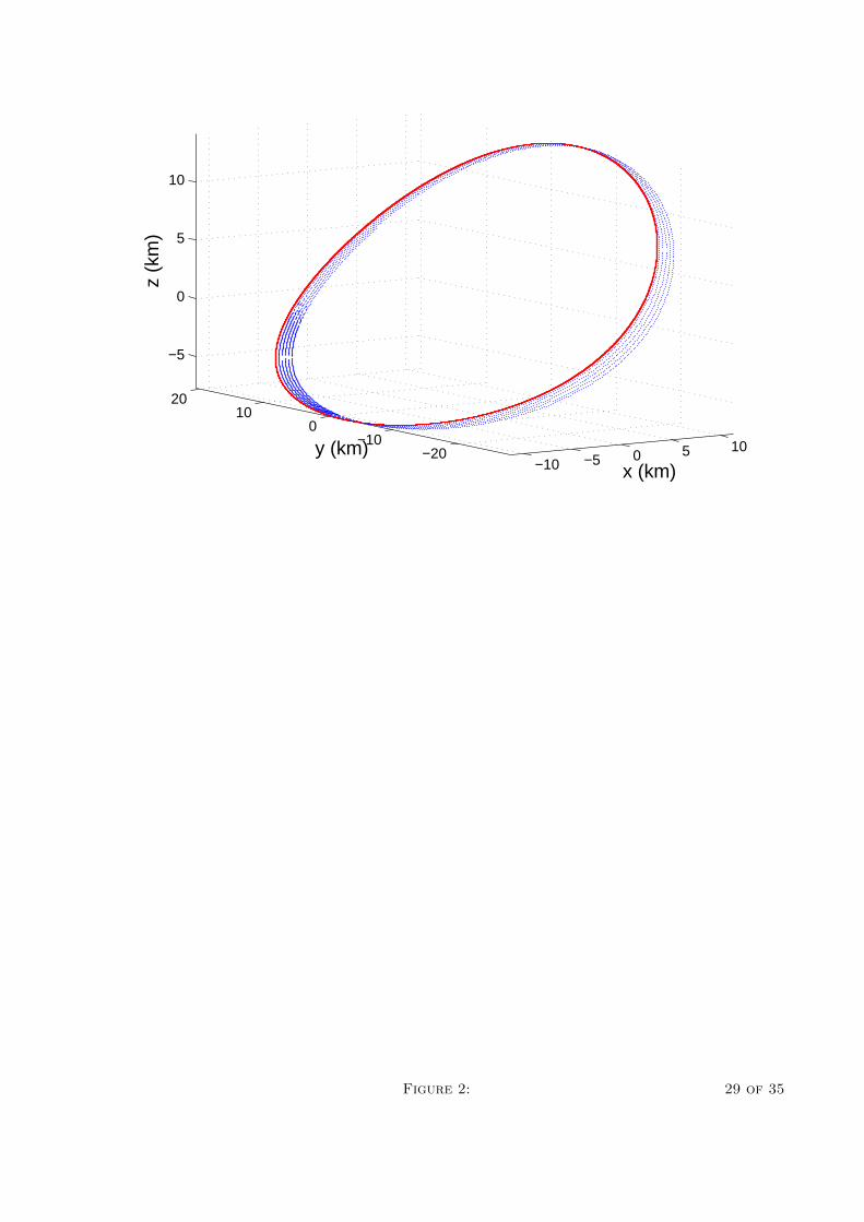
First, the results derived will be used to set up a periodic relative orbit at an arbitrary

epoch. For convenience, nondimensional units are chosen, although the simulations are

based upon dimensional coordinates with time as the independent variable. The initial

true anomaly, orbit size, and eccentricity, are chosen as fi = 105◦, e = 0.3, %0 = 10 km,

respectively. The initial values of the states of the Deputy satellite, denoted by xi, are

chosen from the HCW initial conditions by setting e = 0, ρ1 = ρ3 = 1, ρ2 = 0, and α =

β = 30◦ in Eqs. (21). Therefore, x0i= {0.5 1.732 0.5 0.866 −1 0.866}T (nondimensional).

Equations (20) can be used to obtain their values for a periodic orbit. Upon correction

x′0i= 0.762, y′0i

= −1.331

By using the formulae derived, the correction required to negate secular drift induced by

second-order differential gravity is found to be y′1i= −2.386. The trajectory with and

without this correction is shown in Fig. 2. The broken line indicates the trajectory without

the correction, and considerable drift can be seen after 5 orbits. The solid line indicates that

the corrected trajectory effectively accounts for the second-order differential gravity terms

and remains bounded.

To analyze the extent of efficiency of the correction developed, various cases are drawn

from existing works in the literature. The following cases assume epoch at fi = 0. First,

comparisons are made with the eccentricity/nonlinearity correction from Ref. 20. A reference

orbit with e = 0.05 is chosen with %0 = 10 km. The initial conditions are chosen such that

α = β = 0◦, ρ1 = 2ρ3 = 1, and ρ2 = 0. Figure 3(a) shows the relative orbit using

Hill’s initial conditions (without eccentricity and/or nonlinearity conditions), and using the

correction developed in this paper. The broken line indicates the propagation using the

HCW conditions, for a period of 20 orbits, and it is evident that a large amount of drift

is present. However, by using the corrected initial conditions, the orbit shows negligible

deviation even after 20 orbits. Figure 3(b) shows the percentage drift calculated by using

Eq. (50). It is observed that the uncorrected condition shows about 80% error, which is also

18 of 35

directly observed from Figure 3(a). By using the correction for nonlinearity and eccentricity

developed in Ref. 20, this error is reduced to 10% (correction 1). These errors agree with those

from Ref. 20, for similar initial conditions. By using Eq. (40), this error is approximately

0.2% (correction 2).

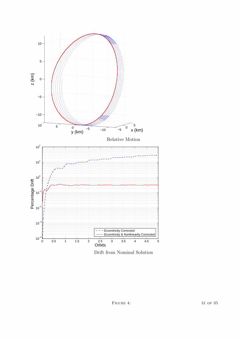
Next, a comparison is made for a reference orbit with moderate eccentricity, where the

result obtained by Ref. 20 fails, but where the zeroth-order eccentricity correction, also

presented by Ref. 18, is expected to be valid. Figure 4(a) shows the relative orbit for e = 0.2

and %0 = 10 km. The Deputy’s orbit is initiated using the periodic equations in Eq. (21),

setting ρ1 = 0.5, ρ2 = 0.1, ρ3 = 1.2, and α = β = 0◦. It is evident that these initial

conditions show secular drift due to nonlinear differential gravity, as indicated by the broken

line. However, by employing the correction derived, the drift is negligible even after 5 orbit

periods, as indicated by the solid line. A study of the drift as shown in Fig. 4(b) shows

that the nonlinearity correction results in an error of approximately 0.3% of the orbit size,

as opposed to the linear condition, which shows approximately 12% drift and continues to

increase.

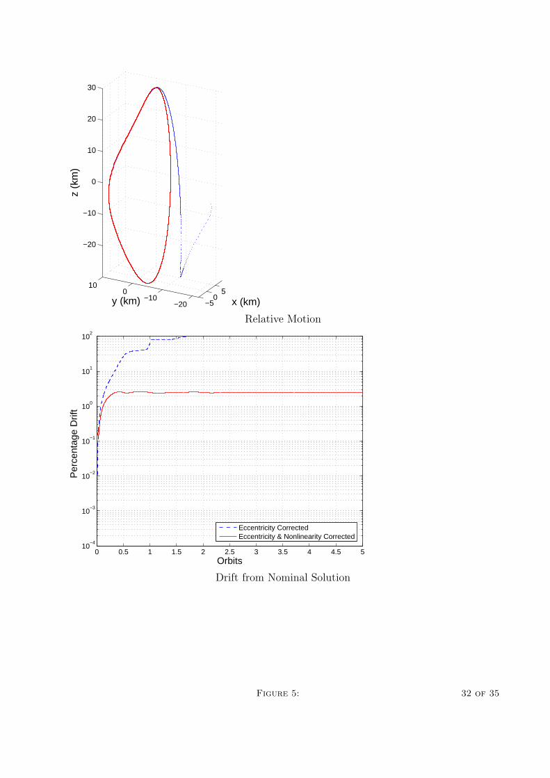
Figure 5(a) shows an orbit with Chief’s eccentricity selected as e = 0.8, all other values

kept the same as in the previous case. In this case it is observed that the initial conditions

that satisfy the linearized periodicity condition do not even lead to bounded motion, and the

relative motion quickly diverges within one orbit period in the presence of nonlinear terms,

as indicated by the broken line. The solid line shows that by using the correction developed

in this paper, periodicity is maintained. As shown in Fig. 5(b), the error after the correction

is approximately 2% of the orbit size. Keeping in mind that the error functions for the

corrected solution, as depicted in Figs. 3(b), 4(b) and 5(b), approach constant values, these

values only indicate the amplitude error as a result of the correction. The orbits themselves

show negligible drift.

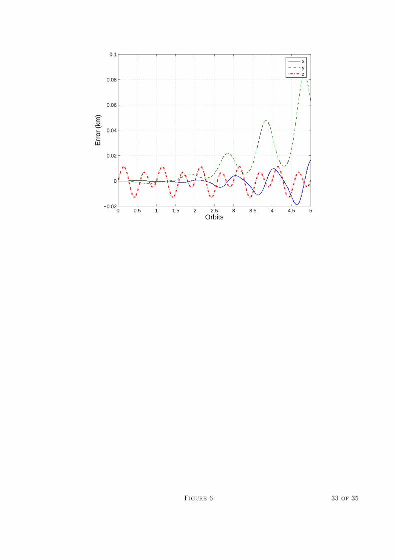
Accuracy of the Analytical Solution

The second-order analytical solution which has been developed in this paper, is tested

against numerical integration in a fully nonlinear differential gravity environment. The

reference orbit has e = 0.4 and a = 12, 000 km. The relative orbit is of dimension %0 =

20 km, and the formation is initiated at fi = 30◦. The parameters for the relative orbit

are: ρ1 = 0.4782, ρ2 = 0.1729, ρ3 = 0.9165, α = −0.5236 and β = −0.5136. The errors

between integrated relative position, and the relative position as predicted by the second-

order analytical equations, is shown in Fig. 6. It is observed that after 5 orbits, the error in

position prediction is within 100m. This is an error of less than 1%. Growth is observed in

the error due to the contribution of terms of third and higher order.

19 of 35

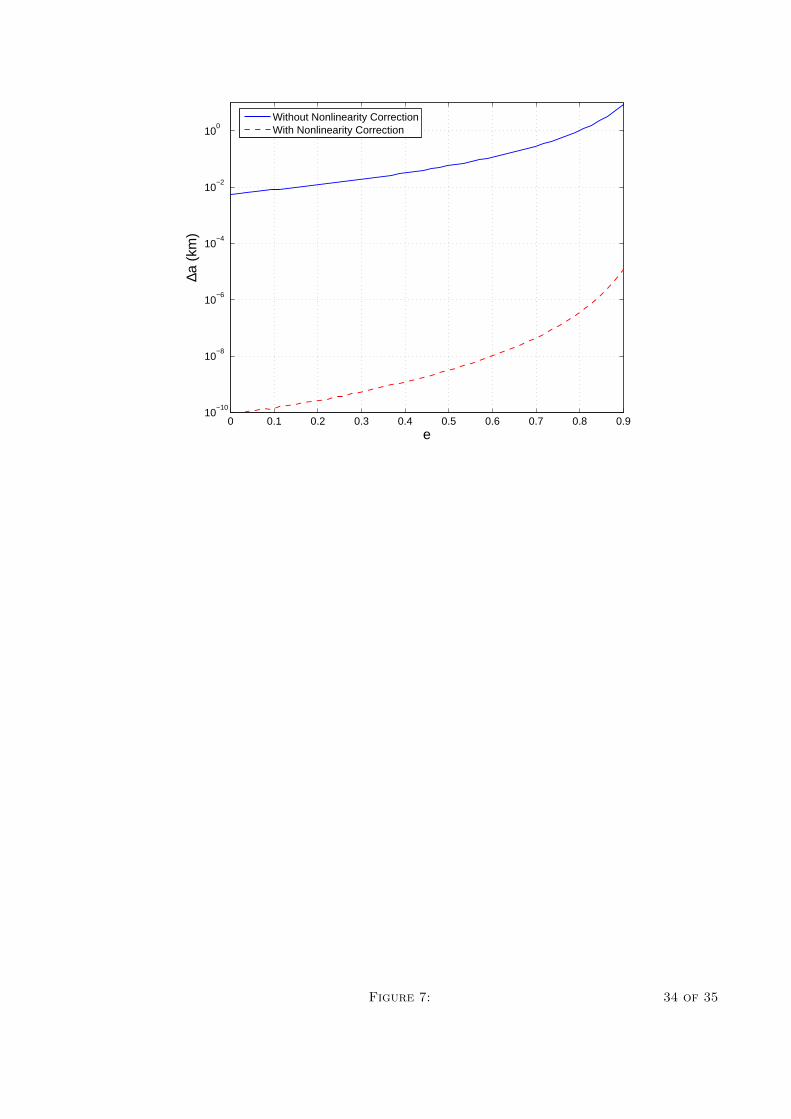
Energy-Matching Criterion

The exact periodicity condition for formation flight is ∆a = 0, or when the time peri-

ods of the Chief and Deputy are equal. However, the periodicity conditions based on the

unperturbed TH equations and the perturbed TH equations, only approximately satisfy the

equation ∆a = 0. The extent to which this condition is satisfied can be measured if the ini-

tial conditions of the Chief’s and Deputy’s states in the local reference frame are converted

to their respective inertial positions and velocities, and then to their respective orbital ele-

ments. A comparison of the uncorrected and nonlinear-corrected initial conditions is shown

in Fig. 7. These results are for a reference orbit with a = 40, 000 km, and %0 = 10 km, with

epoch at fi = 0. It is observed that even if the Chief’s eccentricity is 0.9, the difference

between the Deputy and Chief semi-major axes is of the order of millimeters. Given the

limitations of navigation technology, this is almost exact. In contrast, the uncorrected initial

conditions lead to semi-major axis differences of hundreds of meters even for intermediate

eccentricities, which lead to considerable drift in relative motion.

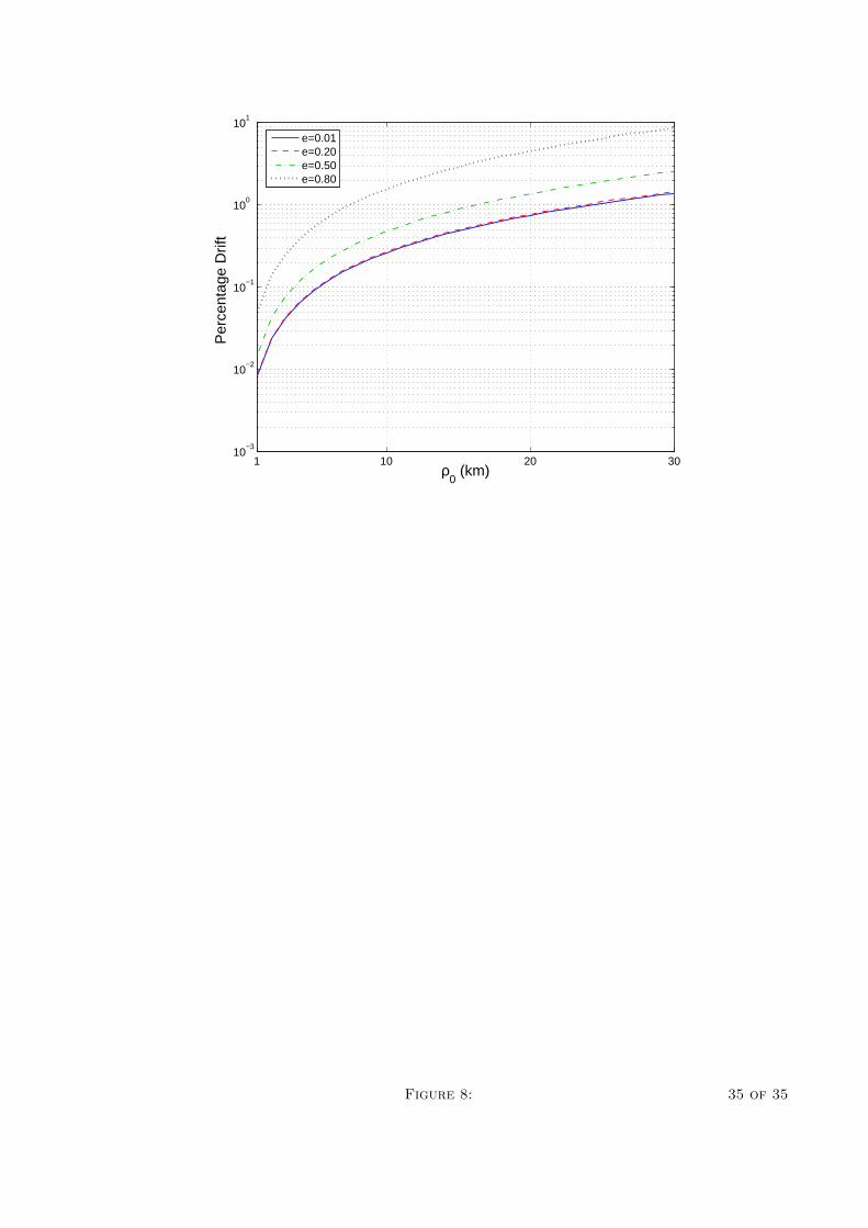
Effect of Eccentricity and Nonlinearity on Boundedness

It is now desired to study the efficacy of the correction under the effect of increasing

%0. This is shown in Fig. 8. These simulations were carried out for 10 time periods of the

reference, for a variety of eccentricity values, as indicated. The figure shows that for %0 up to

30 km, and even with moderate values of eccentricity, the error is less than 1%. However, for

high eccentricities, such as those greater than 0.8, the error is shown to increase markedly.

This is due to the fact that the combined effect of large %0 and large e leads to ε2 and ε

being of the same order, and thus third-order terms in Eq. (12) are no longer negligible in

comparison with the second-order terms.

Conclusions

Phase space initial conditions for periodic relative motion have been developed for an

orbit with arbitrary eccentricity, by treating second-order nonlinear differential gravity terms

as perturbations to the Tschauner-Hempel equations. By identifying only those terms that

contribute to secular growth in relative motion, a condition for ensuring periodic motion is

easily obtained. These initial conditions are shown to work remarkably well under the most

general conditions, including those with very high eccentricities, and can serve as excellent

guesses for initiating a numerical procedure for matching the semi-major axes of the two

satellites by correcting one of the relative motion initial conditions. The removal of secular

growth terms leads to the formulation of analytical, second-order relative motion equations,

that very accurately model relative orbits in terms of its parameters. These expressions can

be used for stationkeeping algorithms and will require less fuel for relative orbit maintenance.

20 of 35

Acknowledgments

The authors wish to thank Kyle T. Alfriend for his help through insightful discussions.

Appendix

Coefficients L0, Lck, Lsk

:

L0 =9e

8ρ2

1 cos 2α + 3ρ1ρ2 cos α

Lc1 = −3

8ρ3

2 cos 2 β − 3

4ρ3

2 +3

4ρ1

2 cos 2 α− 3

2ρ1

2 +3e2

16ρ1

2 +3e

4ρ1ρ2 cos α

−3

2ρ2

2 +e2

4ρ1

2 cos 2 α

Ls1 = − e2

16ρ1

2 sin 2 α +3

8ρ3

2 sin 2 β − 3

4ρ1

2 sin 2 α +3e

4ρ1ρ2 sin α

Lc2 =e

4ρ1

2 cos 2 α, Ls2 = −e

4ρ1

2 sin 2 α

Lc3 =e

4ρ1ρ2 cos α +

1

8ρ3

2 cos 2 β − 1

4ρ1

2 cos 2 α +e2

32ρ1

2 cos 2 α +e2

16ρ1

2

Ls3 = − e2

32ρ1

2 sin 2 α +1

4ρ1

2 sin 2 α− e

4ρ1ρ2 sin α− 1

8ρ3

2 sin 2 β

Lc4 = −e

8ρ1

2 cos 2 α, Ls4 =e

8ρ1

2 sin 2 α

Lc5 = − e2

32ρ1

2 cos 2 α, Ls5 =e2

32ρ1

2 sin 2 α

Evaluating∫

L/ sin2 f df :

∫1

sin2fdf = − cot f

∫sin f

sin2fdf = ln

(1− cos f)

sin f,

∫cos f

sin2fdf = −cosecf

∫sin 2f

sin2fdf = 2 ln sin f,

∫cos 2f

sin2fdf = − cot f − 2f

∫sin 3f

sin2fdf = 4 cos f + 3 ln

(1− cos f)

sin f,

∫cos 3f

sin2fdf = −3 cosecf + 2

cos 2f

sin f∫sin 4f

sin2fdf = 2 cos 2f + 2 + 4 ln sin f,

∫cos 4f

sin2fdf = −2 cot f +

cos 3f

sin f− 4f

∫sin 5f

sin2fdf =

4

3cos 3f + 8 cos f + 5 ln

(1− cos f)

sin f,

∫cos 5f

sin2fdf = −5 cosecf +

2

3

cos 4f

sin f+

10

3

cos 2f

sin f

21 of 35

Evaluating∫

L/φ2 df :

∫1

φ2df = 2eH(f)− 1

φ2

sin 2f

2∫cos f

φ2df = −2

3(2 + e2) H(f) +

1

φ2

[e

6sin 2f − 1

3sin 3f − e

12sin 4f

]

∫cos 2f

φ2df =

2

3e(2 + e2) H(f) +

1

φ2

[−1

esin f − 2

3sin 2f +

1

3esin 3f +

1

12sin 4f

]

∫cos 3f

φ2df = −2(2− e2) H(f) +

1

φ2

[− sin f − e

2sin 2f +

e

4sin 4f

]

∫cos 4f

φ2df = − 2

3e3(8− 24e2 + 13e4) H(f)− 8

e2f +

1

φ2

[4

e3(1 + e2) sin f

+1

6e2(4 + 13e2) sin 2f − 4

3e3(1 + e2) sin 3f − 1

3e2(1 + 4e2) sin 4f

]

∫cos 5f

φ2df = − 2

3e4(−32 + 80e2 − 50e4 + 5e6) H(f) +

32

e3f

+1

φ2

[− 1

e4(16 + 24e2 + e4) sin f − 1

6e3(16 + 96e2 − 5e4) sin 2f

+1

3e4(16 + 24e2 − 5e4) sin 3f +

1

12e3(16 + 96e2 − 5e4) sin 4f + sin 5f

]

(1− e2)2

∫sin f

φ2df =

1

2(1− e)2 ln(1− cos f)− 1

2(1 + e)2 ln(1 + cos f)

+2e ln(1 + e cos f)− e(1− e2)

1 + e cos f

(1− e2)2

∫sin 2f

φ2df = (1− e)2 ln(1− cos f) + (1 + e)2 ln(1 + cos f)

−2(1 + e2) ln(1 + e cos f) +2(1− e2)

1 + e cos f

(1− e2)2

∫sin 3f

φ2df =

3

2(1− e)2 ln(1− cos f)− 3

2(1 + e)2 ln(1 + cos f)

+6e ln(1 + e cos f)− (4− e2)

e

(1− e2)

1 + e cos f

(1− e2)2

∫sin 4f

φ2df = 2(1− e)2 ln(1− cos f) + 2(1 + e)2 ln(1 + cos f)

+4

e2(2− 5e2 + e4) ln(1 + e cos f) +

4(2− e2)

e2

(1− e2)

1 + e cos f

(1− e2)2

∫sin 5f

φ2df =

5

2(1− e)2 ln(1− cos f)− 5

2(1 + e)2 ln(1 + cos f) +

16

e2(1− e2)2 cos f

− 2

e3(16− 32e2 + 11e4) ln(1 + e cos f)− (16− 12e2 + e4)

e3

(1− e2)

1 + e cos f

22 of 35

Coefficients Ck, Dk, Ek, Fk, Gk, Hk:

C1 =e

4ρ2

1 cos 2α + 2ρ1ρ2 cos α +e

2ρ2

1 −1

e

(2ρ2

1 + 2ρ22 + ρ2

3

)

C2 =1

2ρ2

1 cos 2α− 1

4ρ2

3 cos 2β − 1

4

(2ρ2

1 + 2ρ22 + ρ2

3

)

C3 =e

12ρ2

1 cos 2α

D0 = ρ21

(1

4− 1

2e2

)sin 2α +

1

2e2ρ2

3 sin 2β +1

eρ1ρ2 sin α

D1 = ρ21

(e

4− 1

e

)sin 2α +

1

eρ2

3 sin 2β + 2ρ1ρ2 sin α

D2 =1

4ρ2

1 sin 2α

D3 =e

12ρ2

1 sin 2α

E1 = −3e

4ρ2

1 cos 2α− 3ρ1ρ2 cos α, F1 = −3e

4ρ2

1 sin 2α− 3ρ1ρ2 sin α

E2 = −3

4ρ2

1 cos 2α, F2 = −3

4ρ2

1 sin 2α

E3 = − e

12ρ2

1 cos 2α, F3 = − e

12ρ2

1 sin 2α

G1 = D1/2, G2 = D2, G3 = 3D3/2

H0 = − e2

16ρ2

1 cos 2α− e

2ρ1ρ2 cos α +

(1

2− e2

8

)ρ2

1 +1

2ρ2

2 +1

4ρ2

3

H1 = −7e

8ρ2

1 cos 2α− 3ρ1ρ2 cos α− e

8ρ2

3 cos 2β − e

8

(2ρ2

1 + 2ρ22 + ρ2

3

)

H2 = −1

8(4 + e2)ρ2

1 cos 2α− e

2ρ1ρ2 cos α +

1

4ρ2

3 cos 2β +

(1− e2

8

)ρ2

1 + ρ22 +

1

2ρ2

3

H3 = −3e

8ρ2

1 cos 2α +e

8ρ2

3 cos 2β +e

8

(2ρ2

1 + 2ρ22 + ρ2

3

)

H4 = − e2

16ρ2

1 cos 2α

References1Carpenter, J. R., Leitner, J. A., Folta, D. C., and Burns, R. D., “Benchmark Prob-

lems for Spacecraft Formation Flight Missions,” AIAA Guidance, Navigation, and Control

Conference and Exhibit , No. AIAA-2003-5364, AIAA, Austin, TX, August 2003.

2Curtis, S. A., “The Magnetosphere Multiscale Mission... Resolving Fundamental Pro-

cesses in Space Plasmas,” Tech. Rep. NASA TM-2000-209883, NASA Science and Technology

Definition Team for the MMS Mission, 1999.

3Clohessy, W. H. and Wiltshire, R. S., “Terminal Guidance System for Satellite Ren-

23 of 35

dezvous,” Journal of Aerospace Sciences , Vol. 27, September 1960, pp. 653–658, 674.

4Knollman, G. C. and Pyron, B. O., “Relative Trajectories of Objects Ejected from a

Near Satellite,” AIAA Journal , Vol. 1, No. 2, February 1963, pp. 424–429.

5London, H. S., “Second Approximation to the Solution of Rendezvous Equations,”

AIAA Journal , Vol. 1, No. 7, July 1963, pp. 1691–1693.

6Karlgaard, C. D. and Lutze, F. H., “Second-Order Relative Motion Equations,” Journal

of Guidance, Control, and Dynamics , Vol. 26, No. 1, January-February 2003, pp. 41–49.

7Richardson, D. L. and Mitchell, J. W., “A Third-Order Analytical Solution for Relative

Motion with a Circular Reference Orbit,” The Journal of the Astronautical Sciences , Vol. 51,

No. 1, January-March 2003, pp. 1–12.

8Tschauner, J. and Hempel, P., “Rendezvous zu einemin Elliptischer Bahn umlaufenden

Ziel,” Acta Astronautica, Vol. 11, No. 2, 1965, pp. 104–109.

9de Vries, J. P., “Elliptic Elements in Terms of Small Increments of Position and Velocity

Components,” AIAA Journal , Vol. 1, No. 11, November 1963, pp. 2626–2629.

10Kolemen, E. and Kasdin, N. J., “Relative Spacecraft Motion: A Hamiltonian Ap-

proach to Eccentricity Perturbations,” Advances in the Astronautical Sciences , Vol. 119(3),

Paper AAS 04-294 of the AAS/AIAA Spaceflight Mechanics Meeting, Maui, HI, February

2004, pp. 3075–3086.

11Lawden, D. F., Optimal Trajectories for Space Navigation, Butterworths, London, UK,

1967, pp. 79–95.

12Carter, T. E. and Humi, M., “Fuel-Optimal Rendezvous Near a Point in General

Keplerian Orbit,” Journal of Guidance, Control, and Dynamics , Vol. 10, No. 6, November-

December 1987, pp. 567–573.

13Carter, T. E., “New Form for the Optimal Rendezvous Equations Near a Keplerian

Orbit,” Journal of Guidance, Control, and Dynamics , Vol. 13, No. 1, January-February

1990, pp. 183–186.

14Wolfsberger, W., Weiß, J., and Rangnitt, D., “Strategies and Schemes for Rendezvous

on Geostationary Transfer Orbit,” Acta Astronautica, Vol. 10, No. 8, August 1983, pp. 527–

538.

15Yamanaka, K. and Ankersen, F., “New State Transition Matrix for Relative Motion on

an Arbitrary Elliptical Orbit,” Journal of Guidance, Control, and Dynamics , Vol. 25, No. 1,

January-February 2002, pp. 60–66.

16Melton, R. G., “Time Explicit Representation of Relative Motion Between Elliptical

Orbits,” Journal of Guidance, Control and Dynamics , Vol. 23, No. 4, July-August 2000,

pp. 604–610.

24 of 35

17Broucke, R. A., “Solution of the Elliptic Rendezvous Problem with the Time as Inde-

pendent Variable,” Journal of Guidance, Control, and Dynamics , Vol. 26, No. 4, July-August

2003, pp. 615–621.

18Inalhan, G., Tillerson, M., and How, J. P., “Relative Dynamics and Control of Space-

craft Formations in Eccentric Orbits,” Journal of Guidance, Control, and Dynamics , Vol. 25,

No. 1, January-February 2002, pp. 48–59.

19Anthony, M. L. and Sasaki, F. T., “Rendezvous Problem for Nearly Circular Orbits,”

AIAA Journal , Vol. 3, No. 9, September 1965, pp. 1666–1673.

20Vaddi, S. S., Vadali, S. R., and Alfriend, K. T., “Formation Flying: Accommodating

Nonlinearity and Eccentricity Perturbations,” Journal of Guidance, Control, and Dynamics ,

Vol. 26, No. 2, March-April 2003, pp. 214–223.

21Gurfil, P., “Relative Motion Between Elliptic Orbits: Generalized Boundedness Condi-

tions and Optimal Formationkeeping,” Journal of Guidance, Control, and Dynamics , Vol. 28,

No. 4, July-August 2005, pp. 761–767.

22Euler, E. A. and Schulman, Y., “Second-Order Solution to the Elliptic Rendezvous

Problem,” AIAA Journal , Vol. 5, No. 5, May 1967, pp. 1033–1035.

23Alfriend, K. T., Schaub, H., and Gim, D.-W., “Gravitational Perturbations, Non-

linearity and Circular Orbit Assumption Effects on Formation Flying Control Strategies,”

Advances in the Astronautical Sciences , Vol. 104, Paper AAS 00-012 of the AAS Guidance

and Control Conference, Breckenridge, CO, February 2000, pp. 139–158.

24Vadali, S. R., Vaddi, S. S., and Alfriend, K. T., “A New Concept for Controlling

Formation Flying Satellite Constellations,” Advances in the Astronautical Sciences , Vol.

108(2), Paper AAS 01-218 of the AAS/AIAA Spaceflight Mechanics Meeting, Santa Barbara,

CA, February 2001, pp. 1631–1648.

25Schaub, H., “Relative Orbit Geometry Through Classical Orbit Element Differences,”

Journal of Guidance, Control, and Dynamics , Vol. 27, No. 5, September-October 2004,

pp. 839–848.

26Garrison, J. L., Gardner, T. G., and Axelrad, P., “Relative Motion in Highly Ellipti-

cal Orbits,” Advances in the Astronautical Sciences , Vol. 89(2), Paper AAS 95-194 of the

AAS/AIAA Spaceflight Mechanics Meeting, Albuquerque, NM, February 1995, pp. 1359–

1376.

27Sabol, C., McLaughlin, C. A., and Luu, K. K., “Meet the Cluster Orbits with Per-

turbations of Keplerian Elements (COWPOKE) Equations,” Advances in the Astronautical

Sciences , Vol. 114(3), Paper AAS 03-138 of the AAS/AIAA Spaceflight Mechanics Meeting,

Ponce, Puerto Rico, February 2003, pp. 573–594.

25 of 35

28Sengupta, P., Vadali, S. R., and Alfriend, K. T., “Modeling and Control of Satellite

Formations in High Eccentricity Orbits,” The Journal of the Astronautical Sciences , Vol. 52,

No. 1-2, January-June 2004, pp. 149–168.

29Battin, R. H., An Introduction to the Mathematics and Methods of Astrodynamics ,

American Institute of Aeronautics and Astronautics, Inc., Reston, VA, revised ed., 1999,

pp. 110–116, 158–164.

30Alfriend, K. T., Yan, H., and Vadali, S. R., “Nonlinear Considerations in Satellite

Formation Flying,” 2002 AIAA/AAS Astrodynamics Specialist Conference, No. AIAA-2002-

4741, Monterey, CA, August 2002.

31Kechichian, J. A., “Motion in General Elliptic Orbit with Respect to a Dragging and

Precessing Coordinate Frame,” The Journal of the Astronautical Sciences , Vol. 46, No. 1,

January-March 1998, pp. 25–46.

32Nayfeh, A. H., Perturbation Methods , Wiley, Hoboken, NJ, 1973, pp. 23–55.

33Sengupta, P. and Vadali, S. R., “Formation Design and Geometry for Keplerian Ellip-

tic Orbits with Arbitrary Eccentricity,” Paper AAS 06-161 of the AAS/AIAA Spaceflight

Mechanics Meeting, Tampa, FL, January 2006.

26 of 35

List of Figure Captions

Figure 1: Frames of Reference

Figure 2: Corrected and Uncorrected Relative Orbit, e = 0.3, fi = 105◦

Figure 3: Relative Motion with Corrected and Uncorrected Initial Conditions,e = 0.05, fi = 0

a): Relative Motion

b): Drift from Nominal Solution

Figure 4: Relative Motion with Corrected and Uncorrected Initial Conditions,e = 0.2, fi = 0

a): Relative Motion

b): Drift from Nominal Solution

Figure 5: Relative Motion with Corrected and Uncorrected Initial Conditions,e = 0.8, fi = 0

a): Relative Motion

b): Drift from Nominal Solution

Figure 6: Accuracy of the Analytical Solution

Figure 7: Periodicity Condition Satisfaction using Corrected and UncorrectedInitial Conditions

Figure 8: Effect of Nonlinearity and Eccentricity on Errors

27 of 35

f

Periapsis

ir

ihiθ

rC

Referen e Orbit

L

N

ChiefDeputyRelative Orbit

iyix

iz

Figure 1: 28 of 35

−10 −5 0 5 10−20−10

010

20

−5

0

5

10

x (km)y (km)

z (k

m)

Figure 2: 29 of 35

−15 −10 −5 0 5 10

−10

−8

−6

−4

−2

0

2

4

6

8

10

y (km)

z (k

m)

Relative Motion

0 2 4 6 8 10 12 14 16 18 2010

−4

10−3

10−2

10−1

100

101

102

Orbits

Per

cent

age

Drif

t

UncorrectedCorrection 1Correction 2

Drift from Nominal Solution

Figure 3: 30 of 35

−50

5−10−50510

−10

−5

0

5

10

x (km)y (km)

z (k

m)

Relative Motion

0 0.5 1 1.5 2 2.5 3 3.5 4 4.5 510

−4

10−3

10−2

10−1

100

101

102

Orbits

Per

cent

age

Drif

t

Eccentricity CorrectedEccentricity & Nonlinearity Corrected

Drift from Nominal Solution

Figure 4: 31 of 35

−50

5

−20−10

010

−20

−10

0

10

20

30

x (km)y (km)

z (k

m)

Relative Motion

0 0.5 1 1.5 2 2.5 3 3.5 4 4.5 510

−4

10−3

10−2

10−1

100

101

102

Orbits

Per

cent

age

Drif

t

Eccentricity CorrectedEccentricity & Nonlinearity Corrected

Drift from Nominal Solution

Figure 5: 32 of 35

0 0.5 1 1.5 2 2.5 3 3.5 4 4.5 5−0.02

0

0.02

0.04

0.06

0.08

0.1

Orbits

Err

or (

km)

xyz

Figure 6: 33 of 35

0 0.1 0.2 0.3 0.4 0.5 0.6 0.7 0.8 0.910

−10

10−8

10−6

10−4

10−2

100

e

∆a (

km)

Without Nonlinearity CorrectionWith Nonlinearity Correction

Figure 7: 34 of 35

1 10 20 3010

−3

10−2

10−1

100

101

ρ0 (km)

Per

cent

age

Drif

t

e=0.01e=0.20e=0.50e=0.80

Figure 8: 35 of 35