periodic - pearson

CHAPTER TWO

Periodic sampling, the process of representing a continuous signal with a se-quence of discrete data values, pervades the field of digital signal processing.In practice, sampling is performed by applying a continuous signal to an ana-log-to-digital (A/D) converter whose output is a series of digital values. Be-cause sampling theory plays an important role in determining the accuracyand feasibility of any digital signal processing scheme, we need a solid appre-ciation for the often misunderstood effects of periodic sampling. With regardto sampling, the primary concern is just how fast a given continuous signalmust be sampled in order to preserve its information content. We can samplea continuous signal at any sample rate we wish, and we’ll get a series of dis-crete values—but the question is, how well do these values represent the orig-inal signal? Let’s learn the answer to that question and, in doing so, explorethe various sampling techniques used in digital signal processing.

2.1 ALIASING: SIGNAL AMBIGUITY IN THE FREQUENCY DOMAIN

There is a frequency-domain ambiguity associated with discrete-time signalsamples that does not exist in the continuous signal world, and we can appre-ciate the effects of this uncertainty by understanding the sampled nature ofdiscrete data. By way of example, suppose you were given the following se-quence of values,

x(0) = 0x(1) = 0.866x(2) = 0.866x(3) = 0

21

PeriodicSampling 0

0

. . .

. . . . . .

. . .

5725ch02.qxd_cc 2/11/04 8:08 AM Page 21

x(4) = –0.866x(5) = –0.866x(6) = 0 ,

and were told that they represent instantaneous values of a time-domainsinewave taken at periodic intervals. Next, you were asked to draw thatsinewave. You’d start by plotting the sequence of values shown by the dots inFigure 2–1(a). Next, you’d be likely to draw the sinewave, illustrated by thesolid line in Figure 2–1(b), that passes through the points representing theoriginal sequence.

Another person, however, might draw the sinewave shown by theshaded line in Figure 2–1(b). We see that the original sequence of valuescould, with equal validity, represent sampled values of both sinewaves. Thekey issue is that, if the data sequence represented periodic samples of asinewave, we cannot unambiguously determine the frequency of thesinewave from those sample values alone.

Reviewing the mathematical origin of this frequency ambiguity enablesus not only to deal with it, but to use it to our advantage. Let’s derive an ex-pression for this frequency-domain ambiguity and, then, look at a few specificexamples. Consider the continuous time-domain sinusoidal signal defined as

22 Periodic Sampling

Figure 2–1 Frequency ambiguity: (a) discrete-time sequence of values; (b) twodifferent sinewaves that pass through the points of the discrete se-quence.

(a)

(b)

Time

Time

0.866

–0.866

0

5725ch02.qxd_cc 2/11/04 8:08 AM 2

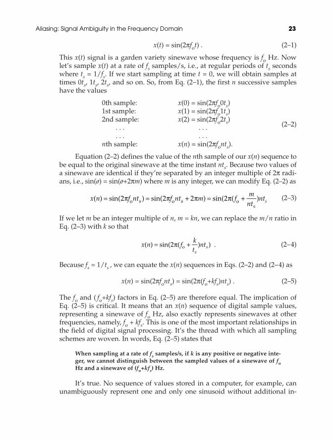
x(t) = sin(2πfot) . (2–1)

This x(t) signal is a garden variety sinewave whose frequency is fo Hz. Nowlet’s sample x(t) at a rate of fs samples/s, i.e., at regular periods of ts secondswhere ts = 1/fs. If we start sampling at time t = 0, we will obtain samples attimes 0ts, 1ts, 2ts, and so on. So, from Eq. (2–1), the first n successive sampleshave the values

0th sample: x(0) = sin(2πfo0ts)1st sample: x(1) = sin(2πfo1ts)2nd sample: x(2) = sin(2πfo2ts) (2–2). . . . . .

. . . . . .nth sample: x(n) = sin(2πfonts).

Equation (2–2) defines the value of the nth sample of our x(n) sequence tobe equal to the original sinewave at the time instant nts. Because two values ofa sinewave are identical if they’re separated by an integer multiple of 2π radi-ans, i.e., sin(ø) = sin(ø+2πm) where m is any integer, we can modify Eq. (2–2) as

(2–3)

If we let m be an integer multiple of n, m = kn, we can replace the m/n ratio inEq. (2–3) with k so that

(2–4)

Because fs = 1/ts , we can equate the x(n) sequences in Eqs. (2–2) and (2–4) as

x(n) = sin(2πfonts) = sin(2π(fo+kfs)nts) . (2–5)

The fo and ( fo+kfs) factors in Eq. (2–5) are therefore equal. The implication ofEq. (2–5) is critical. It means that an x(n) sequence of digital sample values,representing a sinewave of fo Hz, also exactly represents sinewaves at otherfrequencies, namely, fo + kfs. This is one of the most important relationships inthe field of digital signal processing. It’s the thread with which all samplingschemes are woven. In words, Eq. (2–5) states that

When sampling at a rate of fs samples/s, if k is any positive or negative inte-ger, we cannot distinguish between the sampled values of a sinewave of foHz and a sinewave of (fo+kfs) Hz.

It’s true. No sequence of values stored in a computer, for example, canunambiguously represent one and only one sinusoid without additional in-

x n fkt

nts

s( ) sin( ( ) ) .= π +2 o

x n f nt f nt m fm

ntnts s

ss( ) sin( ) sin( ) sin( ( )= π = π + π = π +2 2 2 2o o o

Aliasing: Signal Ambiguity in the Frequency Domain 23

5725ch02.qxd_cc 2/11/04 8:08 AM Page 23

formation. This fact applies equally to A/D-converter output samples as wellas signal samples generated by computer software routines. The sampled na-ture of any sequence of discrete values makes that sequence also represent aninfinite number of different sinusoids.

Equation (2–5) influences all digital signal processing schemes. It’s thereason that, although we’ve only shown it for sinewaves, we’ll see in Chap-ter 3 that the spectrum of any discrete series of sampled values contains peri-odic replications of the original continuous spectrum. The period betweenthese replicated spectra in the frequency domain will always be fs, and thespectral replications repeat all the way from DC to daylight in both directionsof the frequency spectrum. That’s because k in Eq. (2–5) can be any positive ornegative integer. (In Chapters 5 and 6, we’ll learn that Eq. (2–5) is the reasonthat all digital filter frequency responses are periodic in the frequency domainand is crucial to analyzing and designing a popular type of digital filterknown as the infinite impulse response filter.)

To illustrate the effects of Eq. (2–5), let’s build on Figure 2–1 and con-sider the sampling of a 7-kHz sinewave at a sample rate of 6 kHz. A new sam-ple is determined every 1/6000 seconds, or once every 167 microseconds, andtheir values are shown as the dots in Figure 2–2(a).

Notice that the sample values would not change at all if, instead, wewere sampling a 1-kHz sinewave. In this example fo = 7 kHz, fs = 6 kHz, andk = –1 in Eq. (2–5), such that fo+kfs = [7+(–1⋅6)] = 1 kHz. Our problem is that noprocessing scheme can determine if the sequence of sampled values, whoseamplitudes are represented by the dots, came from a 7-kHz or a 1-kHz sinu-soid. If these amplitude values are applied to a digital process that detects en-ergy at 1 kHz, the detector output would indicate energy at 1 kHz. But weknow that there is no 1-kHz tone there—our input is a spectrally pure 7-kHztone. Equation (2–5) is causing a sinusoid, whose name is 7 kHz, to go by thealias of 1 kHz. Asking someone to determine which sinewave frequency ac-counts for the sample values in Figure 2–2(a) is like asking them “When I addtwo numbers I get a sum of four. What are the two numbers?” The answer isthat there is an infinite number of number pairs that can add up to four.

Figure 2–2(b) shows another example of frequency ambiguity, that we’llcall aliasing, where a 4-kHz sinewave could be mistaken for a –2-kHzsinewave. In Figure 2–2(b), fo = 4 kHz, fs = 6 kHz, and k = –1 in Eq. (2–5), sothat fo+kfs = [4+(–1 ⋅ 6)] = –2 kHz. Again, if we examine a sequence of numbersrepresenting the dots in Figure 2–2(b), we could not determine if the sampledsinewave was a 4-kHz tone or a –2-kHz tone. (Although the concept of nega-tive frequencies might seem a bit strange, it provides a beautifully consistentmethodology for predicting the spectral effects of sampling. Chapter 8 dis-cusses negative frequencies and how they relate to real and complex signals.)

Now, if we restrict our spectral band of interest to the frequency range of±fs/2 Hz, the previous two examples take on a special significance. The fre-


5725ch02.qxd_cc 2/11/04 8:08 AM Page 24

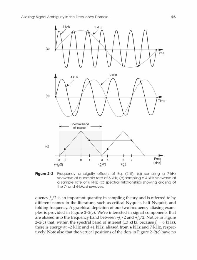
quency fs/2 is an important quantity in sampling theory and is referred to bydifferent names in the literature, such as critical Nyquist, half Nyquist, andfolding frequency. A graphical depiction of our two frequency aliasing exam-ples is provided in Figure 2–2(c). We’re interested in signal components thatare aliased into the frequency band between –fs/2 and +fs/2. Notice in Figure2–2(c) that, within the spectral band of interest (±3 kHz, because fs = 6 kHz),there is energy at –2 kHz and +1 kHz, aliased from 4 kHz and 7 kHz, respec-tively. Note also that the vertical positions of the dots in Figure 2–2(c) have no

Aliasing: Signal Ambiguity in the Frequency Domain 25

Figure 2–2 Frequency ambiguity effects of Eq. (2–5): (a) sampling a 7-kHzsinewave at a sample rate of 6 kHz; (b) sampling a 4-kHz sinewave ata sample rate of 6 kHz; (c) spectral relationships showing aliasing ofthe 7- and 4-kHz sinewaves.

sss

(a)

(b)

(c)

Time

7 kHz 1 kHz

–2 kHz4 kHz

Time

–3 –2 0 1 3 4 6 7 Freq(kHz)

Spectral bandof interest

(f ) (f /2)(–f /2)

5725ch02.qxd_cc 2/11/04 8:08 AM Page 25

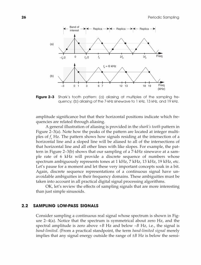
amplitude significance but that their horizontal positions indicate which fre-quencies are related through aliasing.

A general illustration of aliasing is provided in the shark’s tooth pattern inFigure 2–3(a). Note how the peaks of the pattern are located at integer multi-ples of fs Hz. The pattern shows how signals residing at the intersection of ahorizontal line and a sloped line will be aliased to all of the intersections ofthat horizontal line and all other lines with like slopes. For example, the pat-tern in Figure 2–3(b) shows that our sampling of a 7-kHz sinewave at a sam-ple rate of 6 kHz will provide a discrete sequence of numbers whosespectrum ambiguously represents tones at 1 kHz, 7 kHz, 13 kHz, 19 kHz, etc.Let’s pause for a moment and let these very important concepts soak in a bit.Again, discrete sequence representations of a continuous signal have un-avoidable ambiguities in their frequency domains. These ambiguities must betaken into account in all practical digital signal processing algorithms.

OK, let’s review the effects of sampling signals that are more interestingthan just simple sinusoids.

2.2 SAMPLING LOW-PASS SIGNALS

Consider sampling a continuous real signal whose spectrum is shown in Fig-ure 2–4(a). Notice that the spectrum is symmetrical about zero Hz, and thespectral amplitude is zero above +B Hz and below –B Hz, i.e., the signal isband-limited. (From a practical standpoint, the term band-limited signal merelyimplies that any signal energy outside the range of ±B Hz is below the sensi-


Figure 2–3 Shark’s tooth pattern: (a) aliasing at multiples of the sampling fre-quency; (b) aliasing of the 7-kHz sinewave to 1 kHz, 13 kHz, and 19 kHz.

2f 3ff

f = 6 kHz

f /2–f /2

(a)

0

Band ofinterest

(b)

–3 180

Freq

6

s

3 Freq(kHz)

121 7 13 19

s ss s

Replica Replica Replica

s

5725ch02.qxd_cc 2/11/04 8:08 AM Page 26

tivity of our system.) Given that the signal is sampled at a rate of fs samples/s,we can see the spectral replication effects of sampling in Figure 2–4(b), show-ing the original spectrum in addition to an infinite number of replications,whose period of replication is fs Hz. (Although we stated in Section 1.1 thatfrequency-domain representations of discrete-time sequences are themselvesdiscrete, the replicated spectra in Figure 2–4(b) are shown as continuous lines,instead of discrete dots, merely to keep the figure from looking too cluttered.We’ll cover the full implications of discrete frequency spectra in Chapter 3.)

Let’s step back a moment and understand Figure 2–4 for all it’s worth.Figure 2–4(a) is the spectrum of a continuous signal, a signal that can onlyexist in one of two forms. Either it’s a continuous signal that can be sampled,through A/D conversion, or it is merely an abstract concept such as a mathe-matical expression for a signal. It cannot be represented in a digital machine inits current band-limited form. Once the signal is represented by a sequence ofdiscrete sample values, its spectrum takes the replicated form of Figure 2–4(b).

Sampling Low-Pass Signals 27

Figure 2–4 Spectral replications: (a) original continuous signal spectrum; (b)spectral replications of the sampled signal when fs/2 > B; (c) fre-quency overlap and aliasing when the sampling rate is too low be-cause fs/2 < B.

(b)

Freq

. . .. . .

(c)

Freq–2fs

B

f =1.5B

–B

0–fsss f /2s–f /2

2fs

2fs

AliasingAliasing

(a)

Freq0 B–B

0–fs fss f /2s–f /2

B/2–B/2

–2fs

Continuous spectrum

Discrete spectrum

B

. . . . . .

5725ch02.qxd_cc 2/11/04 8:08 AM Page 27

The replicated spectra are not just figments of the mathematics; theyexist and have a profound effect on subsequent digital signal processing.† Thereplications may appear harmless, and it’s natural to ask, “Why care aboutspectral replications? We’re only interested in the frequency band within±fs/2.” Well, if we perform a frequency translation operation or induce achange in sampling rate through decimation or interpolation, the spectralreplications will shift up or down right in the middle of the frequency rangeof interest ±fs/2 and could cause problems[1]. Let’s see how we can controlthe locations of those spectral replications.

In practical A/D conversion schemes, fs is always greater than 2B to sep-arate spectral replications at the folding frequencies of ±fs/2. This very impor-tant relationship of fs ≥ 2B is known as the Nyquist criterion. To illustrate whythe term folding frequency is used, let’s lower our sampling frequency tofs = 1.5B Hz. The spectral result of this undersampling is illustrated in Figure2–4(c). The spectral replications are now overlapping the original basebandspectrum centered about zero Hz. Limiting our attention to the band ±fs/2Hz, we see two very interesting effects. First, the lower edge and upper edgeof the spectral replications centered at +fs and –fs now lie in our band of inter-est. This situation is equivalent to the original spectrum folding to the left at+fs/2 and folding to the right at –fs/2. Portions of the spectral replicationsnow combine with the original spectrum, and the result is aliasing errors. Thediscrete sampled values associated with the spectrum of Figure 2–4(c) nolonger truly represent the original input signal. The spectral information inthe bands of –B to –B/2 and B/2 to B Hz has been corrupted. We show theamplitude of the aliased regions in Figure 2–4(c) as dashed lines because wedon’t really know what the amplitudes will be if aliasing occurs.

The second effect illustrated by Figure 2–4(c) is that the entire spec-tral content of the original continuous signal is now residing in the bandof interest between –fs/2 and +fs/2. This key property was true in Figure2–4(b) and will always be true, regardless of the original signal or thesample rate. This effect is particularly important when we’re digitizing(A/D converting) continuous signals. It warns us that any signal energylocated above +B Hz and below –B Hz in the original continuous spec-trum of Figure 2–4(a) will always end up in the band of interest aftersampling, regardless of the sample rate. For this reason, continuous (ana-log) low-pass filters are necessary in practice.

We illustrate this notion by showing a continuous signal of bandwidth Baccompanied by noise energy in Figure 2–5(a). Sampling this composite con-tinuous signal at a rate that’s greater than 2B prevents replications of the sig-


† Toward the end of Section 5.9, as an example of using the convolution theorem, another de-rivation of periodic sampling’s replicated spectra will be presented.

5725ch02.qxd_cc 2/11/04 8:08 AM Page 28

nal of interest from overlapping each other, but all of the noise energy stillends up in the range between –fs/2 and +fs/2 of our discrete spectrum shownin Figure 2–5(b). This problem is solved in practice by using an analog low-pass anti-aliasing filter prior to A/D conversion to attenuate any unwantedsignal energy above +B and below –B Hz as shown in Figure 2–6. An examplelow-pass filter response shape is shown as the dotted line superimposed onthe original continuous signal spectrum in Figure 2–6. Notice how the outputspectrum of the low-pass filter has been band-limited, and spectral aliasing isavoided at the output of the A/D converter.

This completes the discussion of simple low-pass sampling. Now let’sgo on to a more advanced sampling topic that’s proven so useful in practice.

Sampling Low-Pass Signals 29

Figure 2–5 Spectral replications: (a) original continuous signal plus noise spec-trum; (b) discrete spectrum with noise contaminating the signal of in-terest.

Freq0–fs fss f /2s–f /2

0 B–-B

Noise

Freq

Noise

(a)

(b)

Signal ofinterest

Figure 2–6 Low-pass analog filtering prior to sampling at a rate of fs Hz.

A/DConverter

Analog Low-PassFilter (cutoff

frequency = B Hz)

0 B–B

Noise

Originalcontinuous

signal

Filteredcontinuous signal

Discretesamples

Freq

. . .. . .

0–fs fss f /2s–f /2 2fsFreq

0 B–B Freq

Noise

5725ch02.qxd_cc 2/11/04 8:08 AM Page 29

2.3 SAMPLING BANDPASS SIGNALS

Although satisfying the majority of sampling requirements, the sampling oflow-pass signals, as in Figure 2–6, is not the only sampling scheme used inpractice. We can use a technique known as bandpass sampling to sample a con-tinuous bandpass signal that is centered about some frequency other thanzero Hz. When a continuous input signal’s bandwidth and center frequencypermit us to do so, bandpass sampling not only reduces the speed require-ment of A/D converters below that necessary with traditional low-pass sam-pling; it also reduces the amount of digital memory necessary to capture agiven time interval of a continuous signal.

By way of example, consider sampling the band-limited signal shown inFigure 2–7(a) centered at fc = 20 MHz, with a bandwidth B = 5 MHz. We usethe term bandpass sampling for the process of sampling continuous signalswhose center frequencies have been translated up from zero Hz. What we’recalling bandpass sampling goes by various other names in the literature, suchas IF sampling, harmonic sampling[2], sub-Nyquist sampling, and under-sampling[3]. In bandpass sampling, we’re more concerned with a signal’sbandwidth than its highest frequency component. Note that the negative fre-quency portion of the signal, centered at –fc, is the mirror image of the positivefrequency portion—as it must be for real signals. Our bandpass signal’s high-est frequency component is 22.5 MHz. Conforming to the Nyquist criterion(sampling at twice the highest frequency content of the signal) implies that thesampling frequency must be a minimum of 45 MHz. Consider the effect if thesample rate is 17.5 MHz shown in Figure 2–7(b). Note that the original spectralcomponents remain located at ±fc, and spectral replications are located exactly


Figure 2–7 Bandpass signal sampling: (a) original continuous signal spectrum; (b)sampled signal spectrum replications when sample rate is 17.5 MHz.

0 fc–fc

0 f =c

20 MHz

(a)

(b)

Freq

B =5 MHz

Freq

f = f – B/2 = 17.5 MHzs c

2.5 MHz–2.5 MHz

Bandpass signalspectrum(continuous)

s

s

s

s

–fc

Bandpass signalspectrum (discrete)

f

f

f

f

5725ch02.qxd_cc 2/11/04 8:08 AM Page 30

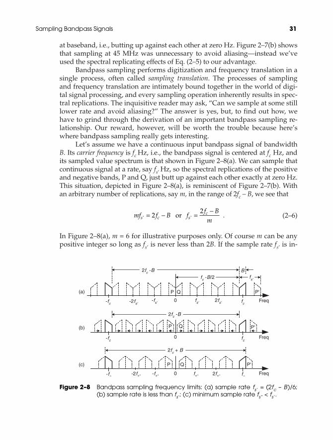
at baseband, i.e., butting up against each other at zero Hz. Figure 2–7(b) showsthat sampling at 45 MHz was unnecessary to avoid aliasing—instead we’veused the spectral replicating effects of Eq. (2–5) to our advantage.

Bandpass sampling performs digitization and frequency translation in asingle process, often called sampling translation. The processes of samplingand frequency translation are intimately bound together in the world of digi-tal signal processing, and every sampling operation inherently results in spec-tral replications. The inquisitive reader may ask, “Can we sample at some stilllower rate and avoid aliasing?” The answer is yes, but, to find out how, wehave to grind through the derivation of an important bandpass sampling re-lationship. Our reward, however, will be worth the trouble because here’swhere bandpass sampling really gets interesting.

Let’s assume we have a continuous input bandpass signal of bandwidthB. Its carrier frequency is fc Hz, i.e., the bandpass signal is centered at fc Hz, andits sampled value spectrum is that shown in Figure 2–8(a). We can sample thatcontinuous signal at a rate, say fs’ Hz, so the spectral replications of the positiveand negative bands, P and Q, just butt up against each other exactly at zero Hz.This situation, depicted in Figure 2–8(a), is reminiscent of Figure 2–7(b). Withan arbitrary number of replications, say m, in the range of 2fc – B, we see that

(2–6)

In Figure 2–8(a), m = 6 for illustrative purposes only. Of course m can be anypositive integer so long as fs’ is never less than 2B. If the sample rate fs’ is in-

mf f B ff Bms c sc

' ' or .= − =−

22

Sampling Bandpass Signals 31

Figure 2–8 Bandpass sampling frequency limits: (a) sample rate fs ’ = (2fc – B )/6;(b) sample rate is less than fs’; (c) minimum sample rate fs” < fs ’.

B

P Q P'

P Q P'

P Q P'

fc -B/22fc -B

fs'

2fc -B

2fc + B

0

0

0

fs' 2fs'-fs' fc-2fs'-fc

fc-fc

fc-fc fs'' 2fs''-fs''-2fs''

(c)

(a)

(b)

Freq

Freq

Freq

5725ch02.qxd_cc 2/11/04 8:08 AM Page 31

creased, the original spectra (bold) do not shift, but all the replications willshift. At zero Hz, the P band will shift to the right, and the Q band will shift tothe left. These replications will overlap and aliasing occurs. Thus, from Eq.(2–6), for an arbitrary m, there is a frequency that the sample rate must not ex-ceed, or

(2–7)

If we reduce the sample rate below the fs’ value shown in Figure 2–8(a), thespacing between replications will decrease in the direction of the arrows inFigure 2–8(b). Again, the original spectra do not shift when the sample rate ischanged. At some new sample rate fs”, where fs’’ < fs’, the replication P’ willjust butt up against the positive original spectrum centered at fc as shown inFigure 2–8(c). In this condition, we know that

(2–8)

Should fs” be decreased in value, P’ will shift further down in frequency andstart to overlap with the positive original spectrum at fc and aliasing occurs.Therefore, from Eq. (2–8) and for m+1, there is a frequency that the samplerate must always exceed, or

(2–9)

We can now combine Eqs. (2–7) and (2–9) to say that fs may be chosen any-where in the range between fs” and fs’ to avoid aliasing, or

(2–10)

where m is an arbitrary, positive integer ensuring that fs ≥ 2B. (For this type ofperiodic sampling of real signals, known as real or first-order sampling, theNyquist criterion fs ≥ 2B must still be satisfied.)

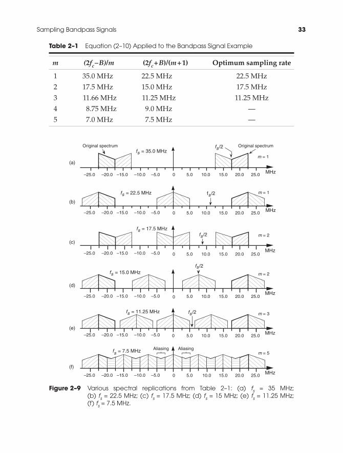
To appreciate the important relationships in Eq. (2–10), let’s return toour bandpass signal example, where Eq. (2–10) enables the generation ofTable 2–1. This table tells us that our sample rate can be anywhere in therange of 22.5 to 35 MHz, anywhere in the range of 15 to 17.5 MHz, or any-where in the range of 11.25 to 11.66 MHz. Any sample rate below 11.25 MHzis unacceptable because it will not satisfy Eq. (2–10) as well as fs ≥ 2B. Thespectra resulting from several of the sampling rates from Table 2–1 are shownin Figure 2–9 for our bandpass signal example. Notice in Figure 2–9(f) thatwhen fs equals 7.5 MHz (m = 5), we have aliasing problems because neither

2 21

f Bm

ff B

mc

sc−

≥ ≥++

,

ff B

msc

" ≥++

21

.

( )m f f B ff B

ms c sc+ = + =

++

1 22

1" " or .

ff Bm

f Bm

fsc c

s' ' or .≤− −

≥2 2


5725ch02.qxd_cc 2/11/04 8:08 AM Page 32


Table 2–1 Equation (2–10) Applied to the Bandpass Signal Example

m (2fc–B)/m (2fc+B)/(m+1) Optimum sampling rate

1 35.0 MHz 22.5 MHz 22.5 MHz

2 17.5 MHz 15.0 MHz 17.5 MHz

3 11.66 MHz 11.25 MHz 11.25 MHz

4 8.75 MHz 9.0 MHz —

5 7.0 MHz 7.5 MHz —

Figure 2–9 Various spectral replications from Table 2–1: (a) fs = 35 MHz; (b) fs = 22.5 MHz; (c) fs = 17.5 MHz; (d) fs = 15 MHz; (e) fs = 11.25 MHz; (f) fs = 7.5 MHz.

(b)

MHz0 5.0 10.0 15.0 20.0 25.0

sf = 22.5 MHz

(f)

0 5.0 10.0 15.0 20.0 25.0 MHz

AliasingAliasingsf = 7.5 MHz

(a)

sf = 35.0 MHz

MHz0 5.0 10.0 15.0 20.0 25.0

f /2s

(c)

MHz0 5.0 10.0 15.0 20.0 25.0

sf = 17.5 MHz

(d)

MHz0 5.0 10.0 15.0 20.0 25.0

sf = 15.0 MHz

(e)MHz0 5.0 10.0 15.0 20.0 25.0

sf = 11.25 MHz

f /2s

f /2s

f /2s

f /2s

Original spectrumOriginal spectrum

m = 1

m = 1

m = 2

m = 2

m = 3

m = 5

–5.0–10.0–15.0–20.0–25.0

–5.0–10.0–15.0–20.0–25.0

–5.0–10.0–15.0–20.0–25.0

–5.0–10.0–15.0–20.0–25.0

–5.0–10.0–15.0–20.0–25.0

–5.0–10.0–15.0–20.0–25.0

5725ch02.qxd_cc 2/11/04 8:08 AM Page 33


the greater than relationships in Eq. (2–10) nor fs ≥ 2B have been satisfied. Them = 4 condition is also unacceptable because fs ≥ 2B is not satisfied. The lastcolumn in Table 2–1 gives the optimum sampling frequency for each accept-able m value. Optimum sampling frequency is defined here as that frequencywhere spectral replications do not butt up against each other except at zeroHz. For example, in the m = 1 range of permissible sampling frequencies, it ismuch easier to perform subsequent digital filtering or other processing on thesignal samples whose spectrum is that of Figure 2–9(b), as opposed to thespectrum in Figure 2–9(a).

The reader may wonder, “Is the optimum sample rate always equal tothe minimum permissible value for fs using Eq. (2–10)?” The answer dependson the specific application—perhaps there are certain system constraints thatmust be considered. For example, in digital telephony, to simplify the follow-on processing, sample frequencies are chosen to be integer multiples of8 kHz[4]. Another application-specific factor in choosing the optimum fs is theshape of analog anti-aliasing filters[5]. Often, in practice, high-performanceA/D converters have their hardware components fine-tuned during manufac-ture to ensure maximum linearity at high frequencies (>5 MHz). Their use atlower frequencies is not recommended.

An interesting way of illustrating the nature of Eq. (2–10) is to plot theminimum sampling rate, (2fc+B)/(m+1), for various values of m, as a functionof R defined as

(2–11)

If we normalize the minimum sample rate from Eq. (2–10) by dividing it bythe bandwidth B, we get a curve whose axes are normalized to the bandwidthshown as the solid curve in Figure 2–10. This figure shows us the minimumnormalized sample rate as a function of the normalized highest frequencycomponent in the bandpass signal. Notice that, regardless of the value of R,the minimum sampling rate need never exceed 4B and approaches 2B as thecarrier frequency increases. Surprisingly, the minimum acceptable samplingfrequency actually decreases as the bandpass signal’s carrier frequency in-creases. We can interpret Figure 2–10 by reconsidering our bandpass signalexample from Figure 2–7 where R = 22.5/5 = 4.5. This R value is indicated bythe dashed line in Figure 2–10 showing that m = 3 and fs/B is 2.25. With B = 5MHz, then, the minimum fs = 11.25 MHz in agreement with Table 2–1. Theleftmost line in Figure 2–10 shows the low-pass sampling case, where thesample rate fs must be twice the signal’s highest frequency component. So thenormalized sample rate fs/B is twice the highest frequency component over Bor 2R.

Rf B

Bc= =

+highest signal frequency componentbandwidth

/ .

2

5725ch02.qxd_cc 2/11/04 8:08 AM Page 34

Figure 2–10 has been prominent in the literature, but its normal presen-tation enables the reader to jump to the false conclusion that any sample rateabove the minimum shown in the figure will be an acceptable samplerate[6–12]. There’s a clever way to avoid any misunderstanding[13]. If weplot the acceptable ranges of bandpass sample frequencies from Eq. (2–10) asa function of R we get the depiction shown in Figure 2–11. As we saw fromEq. (2–10), Table 2–1, and Figure 2–9, acceptable bandpass sample rates are aseries of frequency ranges separated by unacceptable ranges of sample ratefrequencies, that is, an acceptable bandpass sample frequency must be abovethe minimum shown in Figure 2–10, but cannot be just any frequency abovethat minimum. The shaded region in Figure 2–11 shows those normalizedbandpass sample rates that will lead to spectral aliasing. Sample rates withinthe white regions of Figure 2–11 are acceptable. So, for bandpass sampling,we want our sample rate to be in the white wedged areas associated withsome value of m from Eq. (2–10). Let’s understand the significance of Figure2–11 by again using our previous bandpass signal example from Figure 2–7.

Figure 2–12 shows our bandpass signal example R value (highest fre-quency component/bandwidth) of 4.5 as the dashed vertical line. Becausethat line intersects just three white wedged areas, we see that there are onlythree frequency regions of acceptable sample rates, and this agrees with ourresults from Table 2–1. The intersection of the R = 4.5 line and the borders ofthe white wedged areas are those sample rate frequencies listed in Table 2–1.So Figure 2–11 gives a depiction of bandpass sampling restrictions muchmore realistic than that given in Figure 2–10.

Although Figures 2–11 and 2–12 indicate that we can use a sample ratethat lies on the boundary between a white and shaded area, these sample


Figure 2–10 Minimum bandpass sampling rate from Eq. (2–10).

1 2 3 4 5 6 7 8 9 10

4.0

3.5

3.0

2.5

2.0

1.5

f /s BMinimum

RRatio: highest frequency component/bandwidth

m =

1

m

= 2

m = 4m = 5

m = 6m = 7

m = 8

This line corresponds tothe low-pass sampling case,that is, f = 2(f + B/2)s c

m = 3

4.5

2.25

5725ch02.qxd_cc 2/11/04 8:08 AM Page 35

Figure 2–11 Regions of acceptable bandpass sampling rates from Eq. (2–10),normalized to the sample rate over the signal bandwidth (fs/B ).

0

2

4

6

8

10

12

14

2 3 4 5 6 7 8 9 101

Sampling rate (f /B)s

R

m = 1

m = 2

m = 3

2f – Bm

c

2f + Bc

m + 1

Ratio: highest frequency component/bandwidth

f =s

f =s

Shaded region isthe forbidden zone

Figure 2–12 Acceptable sample rates for the bandpass signal example (B = 5MHz) with a value of R = 4.5.

0

2

4

6

8

2 3 4 51 R


f

Bs

= 7, so f = 35 MHzs

f

Bs

= 4.5, so f = 22.5 MHzs

f

Bs

= 3, so f = 15 MHzs

f

Bs

= 2.25, so f = 11.25 MHzs

f

Bs

s

f

Bs

5

3

7


4.5

s

Bandpass signalexample: R = 4.5

= 3.5, so f = 17.5 MHz

= 2.33, so f = 11.66 MHz

36

5725ch02.qxd_cc 2/11/04 8:08 AM Page 36

rates should be avoided in practice. Nonideal analog bandpass filters, samplerate clock generator instabilities, and slight imperfections in available A/Dconverters make this ideal case impossible to achieve exactly. It’s prudent tokeep fs somewhat separated from the boundaries. Consider the bandpasssampling scenario shown in Figure 2–13. With a typical (nonideal) analogbandpass filter, whose frequency response is indicated by the dashed line, it’sprudent to consider the filter’s bandwidth not as B, but as Bgb in our equa-tions. That is, we create a guard band on either side of our filter so that therecan be a small amount of aliasing in the discrete spectrum without distortingour desired signal, as shown at the bottom of Figure 2–13.

We can relate this idea of using guard bands to Figure 2–11 by lookingmore closely at one of the white wedges. As shown in Figure 2–14, we’d liketo set our sample rate as far down toward the vertex of the white area as wecan—lower in the wedge means a lower sampling rate. However, the closerwe operate to the boundary of a shaded area, the more narrow the guardband must be, requiring a sharper analog bandpass filter, as well as thetighter the tolerance we must impose on the stability and accuracy of ourA/D clock generator. (Remember, operating on the boundary between awhite and shaded area in Figure 2–11 causes spectral replications to butt upagainst each other.) So, to be safe, we operate at some intermediate point


Figure 2–13 Bandpass sampling with aliasing occurring only in the filter guardbands.

A/DConverter

BandpassFilter

Digitalsamples

Freq

. . .

0

. . .

fss

Aliasing

0 Freqgb

0

Noise

Freq

Noise

B Filter response

Guard band

gb

Originalcontinuous

signalFiltered

continuous signal

Aliasing

fcfc

fc

f

B

B

5725ch02.qxd_cc 2/11/04 8:08 AM Page 37

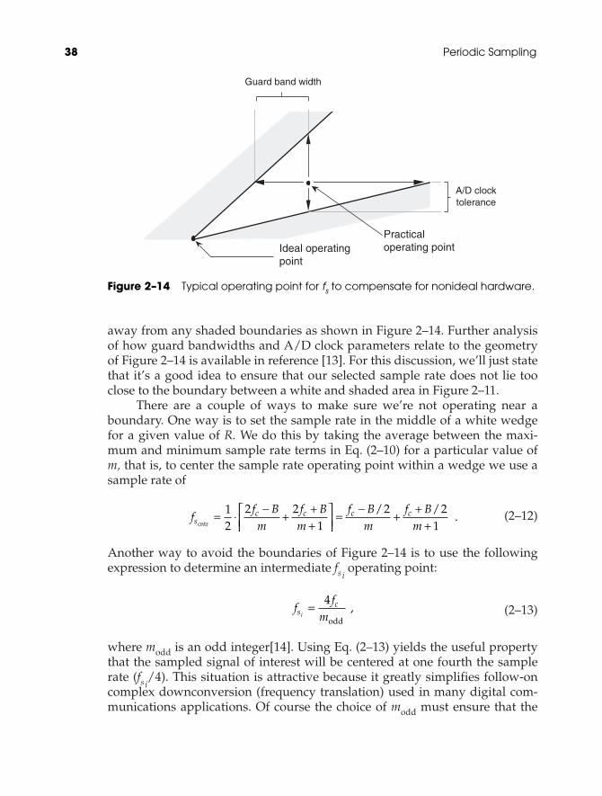
away from any shaded boundaries as shown in Figure 2–14. Further analysisof how guard bandwidths and A/D clock parameters relate to the geometryof Figure 2–14 is available in reference [13]. For this discussion, we’ll just statethat it’s a good idea to ensure that our selected sample rate does not lie tooclose to the boundary between a white and shaded area in Figure 2–11.

There are a couple of ways to make sure we’re not operating near aboundary. One way is to set the sample rate in the middle of a white wedgefor a given value of R. We do this by taking the average between the maxi-mum and minimum sample rate terms in Eq. (2–10) for a particular value ofm, that is, to center the sample rate operating point within a wedge we use asample rate of

(2–12)

Another way to avoid the boundaries of Figure 2–14 is to use the followingexpression to determine an intermediate fsi

operating point:

(2–13)

where modd is an odd integer[14]. Using Eq. (2–13) yields the useful propertythat the sampled signal of interest will be centered at one fourth the samplerate (fsi

/4). This situation is attractive because it greatly simplifies follow-oncomplex downconversion (frequency translation) used in many digital com-munications applications. Of course the choice of modd must ensure that the

ff

msc

i=

4

odd ,

ff Bm

f Bm

f Bm

f Bms

c c c ccntr

= ⋅−

+++

=−

++

+12

2 21

2 21

/ / .


Figure 2–14 Typical operating point for fs to compensate for nonideal hardware.

Guard band width

Practicaloperating pointIdeal operating

point

A/D clocktolerance

5725ch02.qxd_cc 2/11/04 8:08 AM Page 38

Nyquist restriction of fsi> 2B be satisfied. We show the results of Eqs. (2–12)

and (2–13) for our bandpass signal example in Figure 2–15.

2.4 SPECTRAL INVERSION IN BANDPASS SAMPLING

Some of the permissible fs values from Eq. (2–10) will, although avoidingaliasing problems, provide a sampled baseband spectrum (located near zeroHz) that is inverted from the original positive and negative spectral shapes,that is, the positive baseband will have the inverted shape of the negative halffrom the original spectrum. This spectral inversion happens whenever m, inEq. (2–10), is an odd integer, as illustrated in Figures 2–9(b) and 2–9(e). Whenthe original positive spectral bandpass components are symmetrical aboutthe fc frequency, spectral inversion presents no problem and any nonaliasingvalue for fs from Eq. (2–10) may be chosen. However, if spectral inversion issomething to be avoided, for example, when single sideband signals arebeing processed, the minimum applicable sample rate to avoid spectral inver-sion is defined by Eq. (2–10) with the restriction that m is the largest even inte-

Spectral Inversion in Bandpass Sampling 39

Figure 2–15 Intermediate fsi and fscntr operating points, from Eqs. (2–12) and(2–13), to avoid operating at the shaded boundaries for the band-pass signal example. B = 5 MHz and R = 4.5.

f = 28.75 MHz

f = 16.25 MHz

f = 11.46 MHz

cntr

0

2

4

6

8

2 3 4 51 R


Bandpass signalexample: R = 4.5

s

5

3

7


4.5

f = 26.66 MHzs

f = 16.0 MHzs

cntrs

cntrs

f = 11.43 MHzsi

i

i

5725ch02.qxd_cc 2/11/04 8:08 AM Page 39

ger such that fs ≥ 2B is satisfied. Using our definition of optimum samplingrate, the expression that provides the optimum noninverting sampling ratesand avoids spectral replications butting up against each other, except at zeroHz, is

(2–14)

where meven = 2, 4, 6, etc. For our bandpass signal example, Eq. (2–14) andm = 2 provide an optimum noninverting sample rate of fso = 17.5 MHz, asshown in Figure 2–9(c). In this case, notice that the spectrum translated towardzero Hz has the same orientation as the original spectrum centered at 20 MHz.

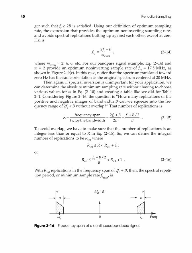
Then again, if spectral inversion is unimportant for your application, wecan determine the absolute minimum sampling rate without having to choosevarious values for m in Eq. (2–10) and creating a table like we did for Table2–1. Considering Figure 2–16, the question is “How many replications of thepositive and negative images of bandwidth B can we squeeze into the fre-quency range of 2fc + B without overlap?” That number of replications is

(2–15)

To avoid overlap, we have to make sure that the number of replications is aninteger less than or equal to R in Eq. (2–15). So, we can define the integralnumber of replications to be Rint where

Rint ≤ R < Rint + 1 ,

or

(2–16)

With Rint replications in the frequency span of 2fc + B, then, the spectral repeti-tion period, or minimum sample rate fsmin

, is

Rf B

BRint int

/ .≤

+< +c 2

1

Rf B

Bf B

Bc c= =

+=

+frequency spantwice the bandwidth

22

2/ .

ff B

msc

o=

−2

even ,


Figure 2–16 Frequency span of a continuous bandpass signal.

2f + Bc

0 fc Freq

B

–fc

B

5725ch02.qxd_cc 2/11/04 8:08 AM Page 40

(2–17)

In our bandpass signal example, finding fsminfirst requires the appropri-

ate value for Rint in Eq. (2–16) as

so Rint = 4. Then, from Eq. (2–17), fsmin= (40+5)/4 = 11.25 MHz, which is the

sample rate illustrated in Figures 2–9(e) and 2–12. So, we can use Eq. (2–17)and avoid using various values for m in Eq. (2–10) and having to create atable like Table 2–1. (Be careful though. Eq. (2–17) places our sampling rate atthe boundary between a white and shaded area of Figure 2–12, and we haveto consider the guard band strategy discussed above.) To recap the bandpasssignal example, sampling at 11.25 MHz, from Eq. (2–17), avoids aliasing andinverts the spectrum, while sampling at 17.5 MHz, from Eq. (2–14), avoidsaliasing with no spectral inversion.

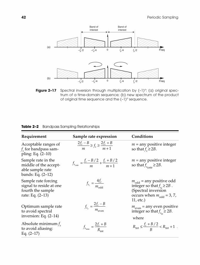
Now here’s some good news. With a little additional digital processing,we can sample at 11.25 MHz, with its spectral inversion and easily reinvertthe spectrum back to its original orientation. The discrete spectrum of anydigital signal can be inverted by multiplying the signal’s discrete-time sam-ples by a sequence of alternating plus ones and minus ones (1, –1, 1, –1, etc.),indicated in the literature by the succinct expression (–1)n. This scheme allowsbandpass sampling at the lower rate of Eq. (2–17) while correcting for spectralinversion, thus avoiding the necessity of using the higher sample rates fromEq. (2–14). Although multiplying time samples by (–1)n is explored in detail inSection 13.1, all we need to remember at this point is the simple rule that mul-tiplication of real signal samples by (–1)n is equivalent to multiplying by a co-sine whose frequency is fs/2. In the frequency domain, this multiplicationflips the positive frequency band of interest, from zero to +fs/2 Hz, about fs/4Hz, and flips the negative frequency band of interest, from –fs/2 to zero Hz,about –fs/4 Hz as shown in Figure 2–17. The (–1)n sequence is not only usedfor inverting the spectra of bandpass sampled sequences; it can be used to in-vert the spectra of low-pass sampled signals. Be aware, however, that, in thelow-pass sampling case, any DC (zero Hz) component in the original continu-ous signal will be translated to both +fs/2 and –fs/2 after multiplication by(–1)n. In the literature of DSP, occasionally you’ll see the (–1)n sequence repre-sented by the equivalent expressions cos(πn) and ejπn.

We conclude this topic by consolidating in Table 2–2 what we need toknow about bandpass sampling.

R Rint int.

,≤ < +22 55

1

ff BRsc

minint

.=+2

Spectral Inversion in Bandpass Sampling 41

5725ch02.qxd_cc 2/11/04 8:08 AM Page 41


Figure 2–17 Spectral inversion through multiplication by (–1)n: (a) original spec-trum of a time-domain sequence; (b) new spectrum of the productof original time sequence and the (–1)n sequence.

(a)

(b)

s f /4s–f /4 0 Freqs f /2s–f /2

s f /4s–f /4 0 Freqs f /2s–f /2

Band ofinterest

Band ofinterest

Table 2–2 Bandpass Sampling Relationships

Requirement Sample rate expression Conditions

Acceptable ranges of m = any positive integer fs for bandpass sam- so that fs ≥ 2B. pling: Eq. (2–10)

Sample rate in the m = any positive integer middle of the accept- so that fscntr

≥ 2B. able sample rate bands: Eq. (2–12)

Sample rate forcing modd = any positive odd signal to reside at one integer so that fsi

≥ 2B . fourth the sample (Spectral inversion rate: Eq. (2–13) occurs when modd = 3, 7,

11, etc.)

Optimum sample rate meven = any even positive to avoid spectral integer so that fso

≥ 2B.inversion: Eq. (2–14)

Absolute minimum fsto avoid aliasing:Eq. (2–17)

where

Rf B

BRc

int int/

.≤+

< +2

1ff BRsc

min=

+2

int

ff B

msc

o=

−2

even

ff

msc

i=

4

odd

ff B

mf B

msc c

cntr=

−+

++

/ /2 21

2 21

f Bm

ff B

mc

sc−

≥ ≥++

5725ch02.qxd_cc 2/11/04 8:08 AM Page 42

REFERENCES

[1] Crochiere, R.E. and Rabiner, L.R. “Optimum FIR Digital Implementations for Decimation,Interpolation, and Narrow-band Filtering,” IEEE Trans. on Acoust. Speech, and Signal Proc.,Vol. ASSP-23, No. 5, October 1975.

[2] Steyskal, H. “Digital Beamforming Antennas,” Microwave Journal, January 1987.

[3] Hill, G. “The Benefits of Undersampling,” Electronic Design, July 11, 1994.

[4] Yam, E., and Redman, M. “Development of a 60-channel FDM-TDM Transmultiplexer,” COMSAT Technical Review, Vol. 13, No. 1, Spring 1983.

[5] Floyd, P., and Taylor, J. “Dual-Channel Space Quadrature-Interferometer System,” Mi-crowave System Designer’s Handbook, Fifth Edition, Microwave Systems News, 1987.

[6] Lyons, R. G. “How Fast Must You Sample,” Test and Measurement World, November 1988.

[7] Stremler, F. Introduction to Communication Systems, Chapter 3, Second Edition, AddisonWesley Publishing Co., Reading, Massachusetts, p. 125.

[8] Webb, R. C. “IF Signal Sampling Improves Receiver Detection Accuracy,” Microwaves &RF, March 1989.

[9] Haykin, S. Communications Systems, Chapter 7, John Wiley and Sons, New York, 1983,p. 376.

[10] Feldman, C. B., and Bennett, W. R. “Bandwidth and Transmission Performance,” Bell SystemTech. Journal, Vol. 28, 1989, p. 490.

[11] Panter, P. F. Modulation Noise, and Spectral Analysis, McGraw-Hill, New York, 1965, p. 527.

[12] Shanmugam, K. S. Digital and Analogue Communications Systems, John Wiley and Sons,New York, 1979, p. 378.

[13] Vaughan, R., Scott, N. and White, D. “The Theory of Bandpass Sampling,” IEEE Trans. onSignal Processing, Vol. 39, No. 9, September 1991, pp. 1973–1984.

[14] Xenakis B., and Evans, A. “Vehicle Locator Uses Spread Spectrum Technology,” RF De-sign, October 1992.

References 43

5725ch02.qxd_cc 2/11/04 8:08 AM Page 43

periodic - pearson

Documents