period changes of ar lacertae between 1900 and 1989aa.springer.de/papers/7326002/2300698.pdf ·...

Astron. Astrophys. 326, 698–708 (1997) ASTRONOMYAND

ASTROPHYSICS

Period changes of AR Lacertae between 1900 and 1989L. Jetsu1, I. Pagano2, D. Moss3, M. Rodono2,4, A.F. Lanza2, and I. Tuominen5

1 NORDITA, Blegdamsvej 17, DK-2100 Copenhagen, Denmark2 Osservatorio Astrofisico di Catania, Citta Universitaria, I-95125, Catania, Italy3 Mathematics Department, The University, Manchester M13 9PL, UK4 Istituto di Astronomia, Universita degli Studi, Viale A. Doria, 6, I-95125 Catania, Italy5 Department of Geosciences and Astronomy, University of Oulu, P.O. Box 333, FIN-90571 Oulu, Finland

Received 6 June 1996 / Accepted 29 April 1997

Abstract. The epochs of the primary and secondary minima ofAR Lac between 1900 and 1989 are analysed with two non-parametric methods of searching for periodicity in a weightedtime point series. An analytical model for transforming theO−C data of eclipsing binaries into the period domain is pre-sented and is applied to AR Lac. The abrupt period changesof AR Lac reported in several previous studies are most prob-ably a consequence of an oversimplified interpretation of theO−C data, since these changes are as likely to be continuous,and even the possibility of a 36y cycle in the period cannot bedefinitely ruled out.

Key words: stars: AR Lacertae – binaries: eclipsing – methods:analytical; statistical

1. Introduction

The following physical parameters are listed for the eclips-ing RS CVn star AR Lac (HR8448, HD210334) in the cata-logue of chromospherically active binaries by Strassmeier etal. (1993): G2iv/K0iv, double–line spectrum with strong CaiiH&K emission from both components, variable Hα emissionand Porb = 1.d983222 ≈ Pphot. The variability of AR Lac wasfirst detected by Leavitt in 1907 (Pickering 1907). A continu-ous light curve is difficult to obtain, because the orbital periodis very close to two days, and hence over two decades elapsed,before Jacchia (1929) found AR Lac to be an eclipsing binary.Since then numerous photometric studies have been made (e.g.see our Table 1) and the geometric, photometric and orbital el-ements of this binary system have been thoroughly examined(e.g. Chambliss 1976, Park 1984, Lee et al. 1986). Hall (1976)published the definition of the RS CVn class of binaries and clas-sified AR Lac as one member of this class. An important detailto remember is his remark that another long period RS CVn

Send offprint requests to: L. Jetsu ([email protected])

star HK Lac (HD 209813, see Blanco & Catalano 1970) wasunfortunately used as a photometric comparison of AR Lac byWood (1946) and Kron (1947), which means that some epochsof the earlier photometric minima may not be very reliable.

Numerous studies of the orbital period variations of ARLac have been made (e.g. Wood 1946, Cester 1967, Chambliss1976, Lee et al. 1986). For example, Kim (1991: his Table 2) de-tected Porb changes between 1.d9831674 and 1.d9832601 (i.e.about 0.d00009). The possible physical phenomena responsi-ble for the period changes of AR Lac have been discussed byHall & Kreiner (1980), and later by, e.g., Panchatsarem & Ab-hyankar (1982) and Kim (1991). The proposed models includemechanisms causing apparent (e.g. photometric starspot distur-bances, light time effect) or real (e.g. rocket effect, mass transferor loss) Porb changes, to mention a few. Most of these modelswere examined with the classical step–technique by Kim (1991),who argued that the correct model to explain the apparentlyabrupt Pobr changes of AR Lac has not yet been found. A moregeneral discussion of the different physical processes that mayexplain the short– and long–term period changes of eclipsingbinaries can be found, e.g., in Hall (1990). A model where theorbital period modulations of eclipsing binaries are connectedto magnetic activity, was quite recently proposed by Applegate(1992), and different types of observational data seem to sup-port several predictions of this model (e.g. Hall 1990, Hall 1991,Rodono et al. 1995). Other recently developed models are massloss (e.g. Verbunt & Hut 1983, van’t Veer & Maceroni 1988,1989, Maceroni & van’t Veer 1991) or mass transfer (Tout &Hall 1991) driven by stellar winds. None of the above modelshas been tested for AR Lac. Our paper presents a method fordetermining the period variations of eclipsing binaries from theepochs of the primary and secondary minima, and this is appliedto the currently available data for AR Lac.

2. Observations

The epochs of the primary and secondary minima of AR Lac inTable 1 were collected from numerous sources. The earliest

L. Jetsu et al.: Period changes of AR Lacertae between 1900 and 1989 699

Table 1. The epochs of the primary and secondary minima of AR Lac [HJD–2400000]: the references are [1]Dugan & Wright (1939), [2]Jacchia(1930), [3]Loreta (1930), [4]Schneller & Plaut (1932), [5]Parenago (1930), [6]Parenago (1938), [7]Rugemer (1931), [8]Zverev (1936), [9]Himpel(1936), [10]Wood (1946), [11]Gainullin (1943), [12]Ahnert (1949), [13]Svechnikov (1955), [14]Wroblewski (1956), [15]Makarov et al. (1957),[16]Karetnikov (1959), [17]Aleksandrovich (1959), [18]Karetnikov (1961), [19]Karle (1962), [20]B.A.N. observers, [21]Oburka (1964), [22]Ahnert(1965), [23]Oburka (1965), [24]Hall (1968), [25]Pohl & Kizilirmak (1966), [26]Ahnert (1966), [27]Kizilirmak & Pohl (1968) [28]Cester (1967),[29]Karle et al. (1977), [30]Pohl & Kizilirmak (1970), [31]Oburka & Silhan (1970), [32]Nha & Kang (1982), [33]Battistini et al. (1973), [34]Pickup(1972), [35]Peter (1972), [36]Kizilirmak & Pohl (1974), [37]Chambliss (1974), [38]Isles (1973), [39]Isles (1975), [40]Pokorny (1974), [41]Scarfe &Barlow (1978), [42]Srivastava (1981), [43]Kurutac et al. (1981), [44]Ertan et al. (1982), [45]Pohl et al. (1982), [46]Park (1984), [47]Caton (1983),[48]Evren et al. (1983), [49]Kim (1991), [50]Pagano (1990), [51]Nezry (1988), [52]Martignoni (1995) and [53]Panov (1987). The notations for differentsystems (v, f, p, pv and e) are explained in the text (Sect. 2). The epochs of the secondary minima are denoted by •

15300.0590[1v] 29404.8470[10e] 38670.4815[22v,23v] 41274.4170[34v] 42319.5750[39v] 44550.6417[46e] 46349.3690[51v]

17005.6490[1v] 29535.7390[10e] 38672.4435[22v,23v] 41506.4430[35v] 42634.8850[29e] 44809.4452[44e,45e]• 46351.3620[51v]

18889.7290[1v] 29692.4110[11f ] 38680.3820[22v] 41513.3920[36e]• 42715.2081[42e]

• 44817.3817[45e]• 46397.9601[49e]

•20991.9730[1v] 32889.3360[12v] 38975.8796[24e] 41592.7219[37e]

• 42716.1968[42e] 44818.3702[45e] 46726.1722[49e]

22995.0380[1v] 34646.4700[13v] 38996.7067[24e]• 41593.7124[37e] 42717.1861[42e]

• 44823.3279[44e]• 46728.1583[49e]

25196.4440[1v] 34888.4290[14v] 39019.5255[25v] 41604.6224[37e]• 43084.0812[32e]

• 44898.6836[47e]• 46738.0734[49e]

25555.4280[2f ] 34890.4060[14v] 39027.4425[20v,26f ] 41635.3860[38v] 43420.2290[32e] 44977.0223[46e] 46742.0394[49e]

25573.2780[3v] 34902.3230[14v] 39029.4260[20v,26f ] 41637.3440[38v] 43427.1700[32e]• 45163.4375[48e] 46745.0181[49e]

•25712.0860[4f ] 36080.3340[15v] 39259.4913[26f,27v] 41639.3505[38v] 43428.1606[32e] 45164.4375[48e]

• 46752.9532[49e]•

25801.3280[5v] 36082.3220[15v] 39376.4926[28e] 41911.0170[39v] 43739.5194[43e] 45165.4189[48e] 47042.5320[52v]•

25803.3200[6v] 36084.3030[15v] 39383.4386[28e]• 41920.9480[39v] 43740.5104[43e]

• 45166.4098[48e]• 47045.5290[52v]

26146.4050[7p] 36766.5250[16v] 39386.4040[26v] 41922.9270[39v] 43745.4701[43e] 45296.3065[48e] 47053.3907[50e,53e]

26489.5260[7p] 36774.4740[16v] 39691.8224[29e] 41936.8022[37e] 43747.4535[43e] 45333.9946[49e] 47054.3796[50e]•

26592.6510[7f ] 36778.4460[16v] 39695.7941[29e] 41938.7874[37e] 43750.4274[43e]• 45337.9580[49e] 47055.3720[53e]

26604.5480[8v] 36784.4175[16v,17v] 39699.7590[29e] 41962.6030[40v] 43751.4182[43e] 45612.6224[50e]• 47056.3610[53e]

•26622.3950[7v] 37137.4410[18v] 39701.7410[29e] 41968.5640[40v] 43752.4108[43e]

• 45674.1062[49e]• 47494.6518[50e]

•26624.3780[7f ] 37569.7977[19e] 39876.2680[30e] 41972.5360[40v] 43755.3858[43e] 45680.0533[49e]

• 47495.6385[50e]

26626.3610[7v] 37623.3320[20v] 40046.8186[29e] 41974.5170[40v] 44113.3584[43e]• 45683.0263[49e] 47733.6202[50e]

26842.5420[4v] 37958.4740[20v] 40443.4710[31v] 42285.8406[29e] 44114.3380[43e] 45691.9558[49e]•

26991.2860[9pv] 38315.4520[21v] 40546.5834[32e] 42287.8274[29e,41e] 44449.4985[44e,45e] 46032.0635[49e]

29178.7610[10e] 38321.3930[21v] 40932.3168[32e,33e]• 42288.8215[29e,41e]

• 44451.4809[44e,45e] 46041.9815[49e]

29186.6930[10e] 38323.3910[20v,21v] 41268.4610[34v] 42289.8120[29e] 44458.4232[44e,45e]• 46344.4039[50e]

•29188.6750[10e] 38333.3450[20v] 41270.4350[34v] 42292.7872[29e]

• 44549.6484[46e]• 46345.4280[51v]

observations were compiled from Hall & Kreiner (1980), andtheir values with zero weights have been omitted. Some modi-fications have been made, the most important being that whenseveral values were available for the same minimum, the valuesin Table 1 are then mean epochs. The original references forthe data denoted by Hall & Kreiner (1980) as “B.B.S.A.G ob-servers” are given, but the first of these values has been omitted(i.e. HJD2440933.330), because it is not listed in the BBSAGBulletin. Although we did not find the original references forthe data referred to as “B.A.N. observers” in Hall & Kreiner(1980), these data have been included in Table 1. The more re-cent observations in Table 1 were compiled from Kim (1991),who revised the epochs of some previously published minima,as well as discarding some values by Srivastava (1981) and Nha& Kang (1982). However, the data by Ishchenko (1963) wereomitted, because Hall & Kreiner (1980) gave zero weights tothese data. The new epochs in Table 1 are from Panov (1987),Nezry (1988), Pagano (1990) and Martignoni (1995).

The data in Table 1 have been obtained with different tech-niques, and we use the notations by Hall & Kreiner (1980):visual estimates (“v”), a series of photographic exposures (“f”),mid-time of exposures on which the object appeared faint (“p”),

a series of measurements with a visual polarizing photometer orsimilar device (“pv”) and, finally, photoelectric measurements(“e”). Because the accuracy of the data is not the same in allsystems and most of the references do not contain an error esti-mate, Hall & Kreiner (1980) gave the weight w = 3 for the “e”data, while observations in all “other” systems were given theweight w = 1. Therefore, the measurements performed in “v”,“f”, “p” and “pv” are also referred to as “other” systems in thispaper. For reasons to be discussed later (see Table 3), our errorestimates are σe =0.d004 and σother =0.d011.

3. The ephemeris of AR Lac

The standard technique to determine the ephemerides of eclips-ing binaries is to make linear or quadratic least squares fits to theO−C data. This procedure has been applied for AR Lac, e.g.,by Chambliss (1976) and Hall & Kreiner (1980). Even higherorder polynomials have been used in deriving the O−C data ofsome eclipsing binaries. For example, Wood & Forbes (1963)derived ephemerides based on third order polynomials. In thispaper the ephemeris of AR Lac is determined with two non-parametric methods of searching for periodicity in a weightedtime point series, presented by Jetsu & Pelt (1996: hereafter Pa-

700 L. Jetsu et al.: Period changes of AR Lacertae between 1900 and 1989

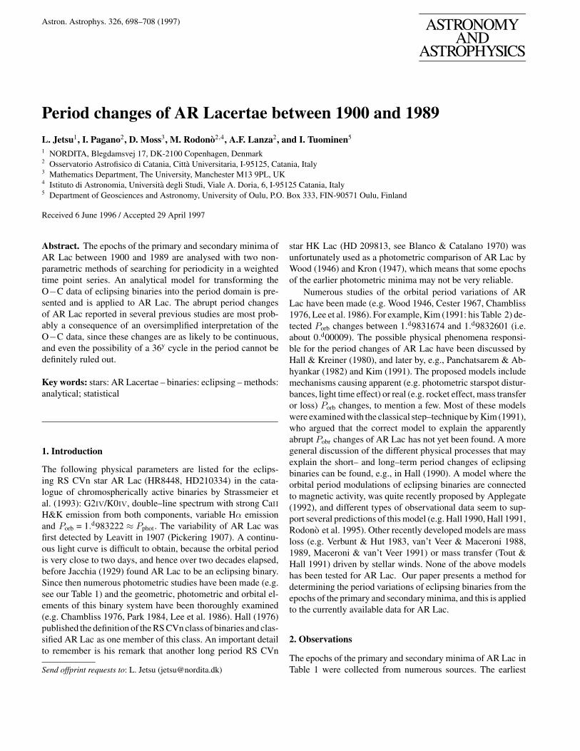
Fig. 1. a The O−C variations of AR Lac with the ephemeris (1): primary minima (“e”≡ closed squares, “other” ≡ open squares), secondaryminima (“e”≡ closed circles, “other” ≡ open circles). The (O−C)(T, P0) curves (Eq. 3: Ci(P0) from Table 2) for K =8 (dotted line) and K =9(continuous line) and their 1σ error limits (Eq. 5). The assigned errors in “e” (±0.d004≈±0.0020 in phase) and “other” (±0.d011≈±0.0055in phase) are shown separately in the lower right corner. b The total range of 1σ error limits of (O−C)(T, P0). c The O−C distribution in binsof 0.02 for the “e” (dark) and “other” data (white)

per i), which were already applied in Jetsu (1996) and Jetsu etal. (1997). Our Appendix summarizes the necessary informationof the WK– and WSD–methods, as well as the determinationof the following two ephemerides

HJD2415298.321(±.003)+1.983208(±.000006)EWK (1)

HJD2415298.646(±.005)+1.983184(±.000007)EWSD. (2)

The O−C variations for (1) and (2) are shown in Figs. 1a and 2a,where 0.5 has been subtracted from the O−C values of the sec-ondary minima to shift them to the level of the primary minima.Note that the unit of the O−C data is phases (i.e. not days), be-cause these phases represent circular data (see Appendix) andthus the modelling presented below is formulated for phases.

4. The model

The determination of an ephemeris for an eclipsing binary doesnot represent an analysis of Porb changes, but only yields theperiod P0 that minimizes the O−C residuals with respect to a

linear or higher order least squares fit for the whole data (e.g.Hall & Kreiner 1980 for AR Lac). The classical technique tostudy Porb changes (i.e. the “step–technique”), is to determinelinear least squares fits for parts of the O−C data, and the previ-ous studies of AR Lac contain examples of this approach (e.g.Chambliss 1976, Kim 1991). Another technique is to obtainhigher order polynomial least squares fits for the whole or partsof the O−C data (Kalimeris et al. 1994ab, 1995), and this type ofa technique is hereafter referred to as “continuous–technique”.

One alternative continuous–technique for modelling of theperiod changes from the epochs of the primary and secondaryminima of eclipsing binaries is presented in this section, and theresults for AR Lac are discussed. The possible physical inter-pretations of these results are presented separately in Sect. 5.2.Although a thorough comparison between our method and thatby Kalimeris et al. (1994ab, 1995) is not presented, we wishto emphasize the following two main differences. Firstly, theO−C data are analysed in phase domain, while Kalimeris etal. formulated their method in the time domain. Secondly, the


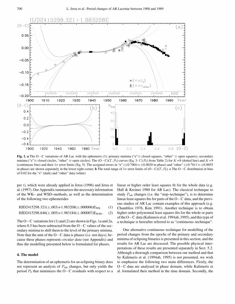
Fig. 2. The same as Fig. 1, using the ephemeris (2)

period changes are solved directly from the free parameters ofthe model (i.e. Ci of Eq. 3). As for the main similarities, the so-lution forPorb changes is independent of the value ofP0 appliedin deriving the O−C data for both methods (see Kalimeris etal. 1994b: Appendix I, and Eq. 7 in our paper). Furthermore,when the whole O−C data could not be adequately modelledwith one polynomial fit, Kalimeris et al. (1994ab) correctly em-phasized the uncertainties connected with the modelling of thedata in parts. In such cases, they ascertained the continuity of theO−C modelling by spline interpolation. Except for SZ Piscium(Kalimeris et al. 1995), the orbital period changes of no otherRS CVn system have been studied earlier with a continuous–technique.

4.1. The O−C variations

Before modelling of the O−C data of AR Lac with higher or-der polynomials (i.e. Eq. 3 below), we briefly discuss how thestep–technique could be applied to these data. For example, vi-sual inspection might suggest that the variations in Fig. 1a couldbe adequately presented by five or six linear fits, which wouldmore or less resemble the step–technique applied by Kim (1991:his Fig. 1). On the other hand, perhaps four or five linear fits

might suffice for rough modelling of Fig. 2a. The interpretationswould then be that the period has been decreasing from the be-ginning of 1960 (Fig. 1a), or increasing from the beginning ofthe century to 1980 (Fig. 2a). One might even claim that Fig. 1amay indicate periodicity in the O−C variations. But the mainproblem with these interpretations is that abrupt and discontin-uous period changes seem to occur at the epochs where the linesfitted to the O−C data intersect. Furthermore, there is plenty offreedom in choosing the intervals for fitting. Unfortunately, theresults of the step–technique also depend on the chosen P0 toderive the O−C values.

In reality, the function for modelling the O−C data is un-known. Furthermore, the shape of this function depends on P0.The models for the O−C data shown in Figs. 1a and b and 2aand b are

(O−C)(T, P0) =K∑

i=0

Ci(P0)T i, (3)

where K = 8 or 9. The standard least squares fit method wasapplied to solve the best values for the free parameters C0(P0),..., CK(P0). The time scale is T = (t − t′′)/Tscale, where t′′ =HJD2431516.8396 is the mid point of the time interval of the


data and time is transformed into centuries by Tscale = 36525(i.e. −1 < T < 1), which simplifies the computation of thefree parameters for higher order models. The values C0(P0), ...,CK(P0) for the curves in Fig. 1a and b are given in Table 2.A simple connection exists between the models (Eq. 3) for thedata in Figs. 1a and b, and 2a and b, because the transformationbetween them is

(O−C)(T, P1)−(O−C)(T, P2) =P2 − P1

P1P2T+

P1T2 − P2T1

P1P2, (4)

where T1 and P1, and T2 and P2 are the zero points and periodsof the ephemerides (1) and (2), respectively. The model givesdifferent values only for C0(P0) and C1(P0), while values ofC2(P0), ..., CK(P0) are the same for P0 =P1 and P2. The coef-ficients on the right side of Eq. 4 determine the differences inC0(P0) and C1(P0). Although the O−C variations in Figs. 1aand 2a do not appear similar, Eq. 4 shows that the model doesnot strongly depend on the choice of P0.

Why should the model of Eq. 3 be better than some morearbitrary model? What is the reason for choosing K = 8 or 9in Figs. 1a and b, and 2a and b? The answer to the first ques-tion is that whatever the form of the unknown function suitablefor modelling the O−C data, it can be expanded in a Taylorseries, unless it or its derivatives are discontinuous. The coeffi-cients of Eq. 3 can be interpreted as coefficients of the Taylorexpansion of this unknown function. In conclusion, this is allthe information that can be extracted from the O−C data withan unknown model. The O−C variations of AR Lac may in-deed be discontinuous, but the observations in “e” system cer-tainly do not suggest this (Figs. 1a and 2a: closed symbols). Itrather seems that the accuracy of the data in “other” systems isrelatively low. While the continuity of the O−C curve of ARLac can not be proved beyond doubt, we will continue by as-suming that this is the case. Some physical considerations arealso mentioned in connection with Eqs. 6 and 7. The 1σ errorlimits for (O−C)(T, P0) in this model (Eq. 3) are

σO−C(T, P0) =

√√√√ K∑i=0

(T iσCi )2, (5)

where σCi are the 1σ errors of the free parameters Ci(P0). Be-cause only a Taylor expansion of the unknown model is avail-able, these error estimates diverge strongly at both ends of thetime interval of the data, as shown in Figs. 1b and 2b.

The question of choosing the order (K) in Eq. 3 can besettled by setting all weights to unity and modelling Eq. 3 todifferent orders. The mean residuals given in Table 3 stop de-creasing at K = 9 for both the “e” and the “other” data. Thesemean residuals with weights of unity should satisfy an approx-imation 〈σe〉 ≈ 〈εe〉 = 0.d004 and 〈σother〉 ≈ 〈εother〉 = 0.d011(see, e.g., Press et al. 1986) and thus they were chosen as errorestimates for the data in Table 1. Inspection of Table 3 also re-veals that it is unnecessary to model the data in higher orders(i.e. K>9), because the mean residuals will not decrease. Theweighted modelling for K = 9 with the above error estimates

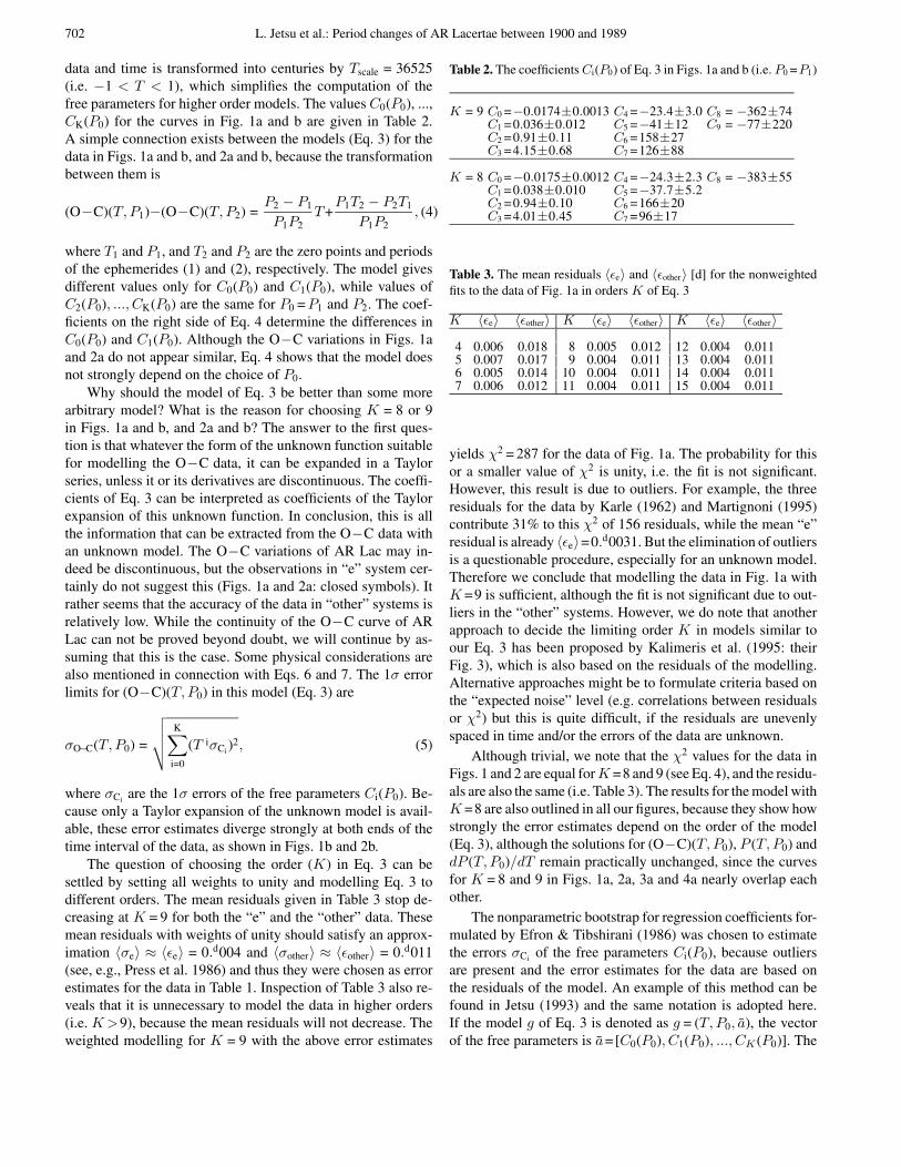
Table 2. The coefficientsCi(P0) of Eq. 3 in Figs. 1a and b (i.e. P0 =P1)

K = 9 C0 =−0.0174±0.0013 C4 =−23.4±3.0 C8 = −362±74C1 =0.036±0.012 C5 =−41±12 C9 = −77±220C2 =0.91±0.11 C6 =158±27C3 =4.15±0.68 C7 =126±88

K = 8 C0 =−0.0175±0.0012 C4 =−24.3±2.3 C8 = −383±55C1 =0.038±0.010 C5 =−37.7±5.2C2 =0.94±0.10 C6 =166±20C3 =4.01±0.45 C7 =96±17

Table 3. The mean residuals 〈εe〉 and 〈εother〉 [d] for the nonweightedfits to the data of Fig. 1a in orders K of Eq. 3

K 〈εe〉〈εother〉 K 〈εe〉〈εother〉 K 〈εe〉〈εother〉4 0.006 0.018 8 0.005 0.012 12 0.004 0.0115 0.007 0.017 9 0.004 0.011 13 0.004 0.0116 0.005 0.014 10 0.004 0.011 14 0.004 0.0117 0.006 0.012 11 0.004 0.011 15 0.004 0.011

yields χ2 = 287 for the data of Fig. 1a. The probability for thisor a smaller value of χ2 is unity, i.e. the fit is not significant.However, this result is due to outliers. For example, the threeresiduals for the data by Karle (1962) and Martignoni (1995)contribute 31% to this χ2 of 156 residuals, while the mean “e”residual is already 〈εe〉=0.d0031. But the elimination of outliersis a questionable procedure, especially for an unknown model.Therefore we conclude that modelling the data in Fig. 1a withK =9 is sufficient, although the fit is not significant due to out-liers in the “other” systems. However, we do note that anotherapproach to decide the limiting order K in models similar toour Eq. 3 has been proposed by Kalimeris et al. (1995: theirFig. 3), which is also based on the residuals of the modelling.Alternative approaches might be to formulate criteria based onthe “expected noise” level (e.g. correlations between residualsor χ2) but this is quite difficult, if the residuals are unevenlyspaced in time and/or the errors of the data are unknown.

Although trivial, we note that the χ2 values for the data inFigs. 1 and 2 are equal forK =8 and 9 (see Eq. 4), and the residu-als are also the same (i.e. Table 3). The results for the model withK =8 are also outlined in all our figures, because they show howstrongly the error estimates depend on the order of the model(Eq. 3), although the solutions for (O−C)(T, P0), P (T, P0) anddP (T, P0)/dT remain practically unchanged, since the curvesfor K = 8 and 9 in Figs. 1a, 2a, 3a and 4a nearly overlap eachother.

The nonparametric bootstrap for regression coefficients for-mulated by Efron & Tibshirani (1986) was chosen to estimatethe errors σCi of the free parameters Ci(P0), because outliersare present and the error estimates for the data are based onthe residuals of the model. An example of this method can befound in Jetsu (1993) and the same notation is adopted here.If the model g of Eq. 3 is denoted as g = (T, P0, a), the vectorof the free parameters is a=[C0(P0), C1(P0), ..., CK(P0)]. The


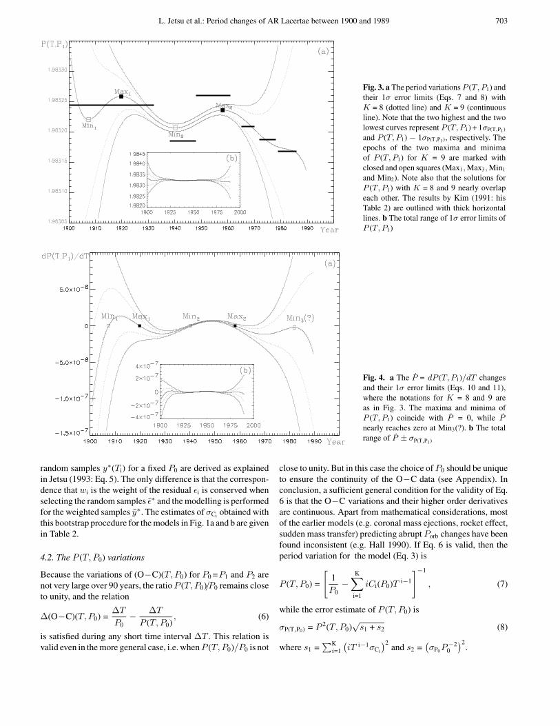
Fig. 3. a The period variations P (T, P1) andtheir 1σ error limits (Eqs. 7 and 8) withK = 8 (dotted line) and K = 9 (continuousline). Note that the two highest and the twolowest curves represent P (T, P1) + 1σP(T,P1)

and P (T, P1) − 1σP(T,P1), respectively. Theepochs of the two maxima and minimaof P (T, P1) for K = 9 are marked withclosed and open squares (Max1,Max3,Min1

and Min2). Note also that the solutions forP (T, P1) with K = 8 and 9 nearly overlapeach other. The results by Kim (1991: hisTable 2) are outlined with thick horizontallines. b The total range of 1σ error limits ofP (T, P1)

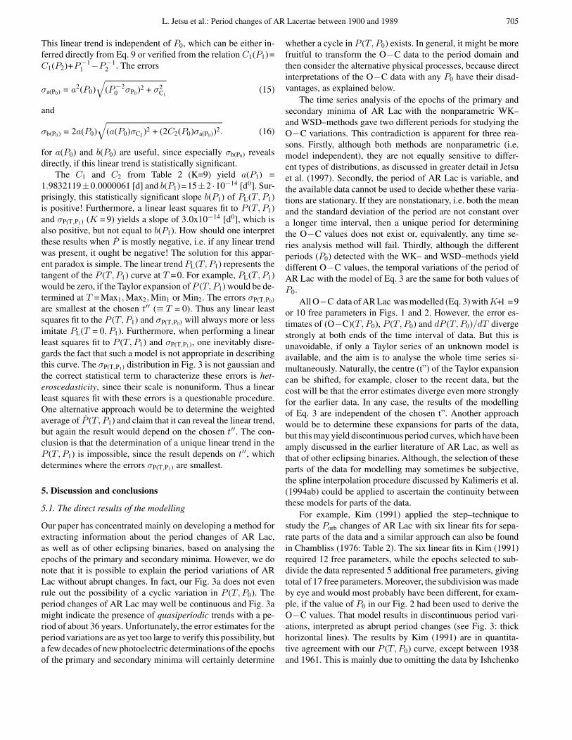
Fig. 4. a The P = dP (T, P1)/dT changesand their 1σ error limits (Eqs. 10 and 11),where the notations for K = 8 and 9 areas in Fig. 3. The maxima and minima ofP (T, P1) coincide with P = 0, while Pnearly reaches zero at Min3(?). b The totalrange of P ± σP(T,P1)

random samples y∗(Ti) for a fixed P0 are derived as explainedin Jetsu (1993: Eq. 5). The only difference is that the correspon-dence that wi is the weight of the residual εi is conserved whenselecting the random samples ε∗ and the modelling is performedfor the weighted samples y∗. The estimates of σCi obtained withthis bootstrap procedure for the models in Fig. 1a and b are givenin Table 2.

4.2. The P (T, P0) variations

Because the variations of (O−C)(T, P0) for P0 =P1 and P2 arenot very large over 90 years, the ratioP (T, P0)/P0 remains closeto unity, and the relation

∆(O−C)(T, P0) =∆T

P0− ∆T

P (T, P0), (6)

is satisfied during any short time interval ∆T . This relation isvalid even in the more general case, i.e. whenP (T, P0)/P0 is not

close to unity. But in this case the choice ofP0 should be uniqueto ensure the continuity of the O−C data (see Appendix). Inconclusion, a sufficient general condition for the validity of Eq.6 is that the O−C variations and their higher order derivativesare continuous. Apart from mathematical considerations, mostof the earlier models (e.g. coronal mass ejections, rocket effect,sudden mass transfer) predicting abrupt Porb changes have beenfound inconsistent (e.g. Hall 1990). If Eq. 6 is valid, then theperiod variation for the model (Eq. 3) is

P (T, P0) =

[1P0

−K∑

i=1

iCi(P0)T i−1

]−1

, (7)

while the error estimate of P (T, P0) is

σP(T,P0) = P 2(T, P0)√s1 + s2 (8)

where s1 =∑K

i=1

(iT i−1σCi

)2and s2 =

(σP0P

−20

)2.


The transformation of Eq. 4 shows that the difference betweenthe coefficients C1(P1) and C1(P2) for the model of Eq. 3 isP−1

1 −P−12 . Because all other coefficients C2(P0), ..., CK(P0)

are equal for both periods, it is quite easy to show that

P (T, P1) = P (T, P2). (9)

In conclusion, the results for the period variations are the samefor the O−C data of Figs. 1 and 2.

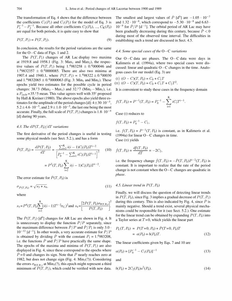
The P (T, P1) changes of AR Lac display two maximaat 1919.8 and 1958.1 (Fig. 3: Max1 and Max2), the respec-tive values of P (T, P1) being 1.d983258 ± 0.d000046 and1.d9832357 ± 0.d0000085. There are also two minima at1907.4 and 1940.1, where P (T, P1) = 1.d98322± 0.d00030and 1.d9832065± 0.d0000063 (Fig. 3: Min1 and Min2). Theseepochs yield two estimates for the possible cycle in periodchanges: 38.y3 (Max2−Max1) and 32.y7 (Min2−Min1), i.e.a Pcycle =35.y5 mean. This value agrees well with 35y proposedby Hall & Kreiner (1980). The above epochs also yield three es-timates for the amplitude of the period changes [d]: 4±30·10−5,5.2±4.6 ·10−5, and 2.9±1.0 ·10−5, the last one being the mostaccurate. Finally, the full scale ofP (T, P1) changes is 1.8 ·10−4

[d] during 90 years.

4.3. The dP (T, P0)/dT variations

The first derivative of the period changes is useful in testingsome physical models (see Sect. 5.2.), and has a form

P (T, P0) =dP (T, P0)

dT=

∑Ki=2 i(i− 1)Ci(P0)T i−2[

P−10 −∑K

i=1 iCi(P0)T i−1]2 (10)

= P 2(T, P0)K∑

i=2

i(i− 1)Ci(P0)T i−2.

The error estimate for P (T, P0) is

σP (T,P0) =√s3 + s4, (11)

where

s3 =P 4(T, P0)K∑

i=2

(i(i−1)T i−2σCi )2and s4 =

[2P (T, P0)σP(T,P0)

P (T, P0)

]2.

The P (T, P1) [d0] changes for AR Lac are shown in Fig. 4. Itis unnecessary to display the function P /P separately, sincethe maximum difference between P /P and P /P1 is only 3.0 ·10−12 [d−1]. In other words, a very accurate estimate for P /Pis obtained by dividing P with the constant P1 = 1.d983208,i.e. the functions P and P /P have practically the same shape.The epochs of the maxima and minima of P (T, P1) are alsodisplayed in Fig. 4, since these correspond to the epochs whereP = 0 and changes its sign. Note that P nearly reaches zero at1982, but does not change sign (Fig. 4: Min3(?)). Consideringthe errors σP(T,P1) at Min3(?), this epoch might represent a thirdminimum of P (T, P1), which could be verified with new data.

The smallest and largest values of P [d0] are −1.05 · 10−7

and 1.32 · 10−8, which correspond to −5.30 · 10−8 and 6.63 ·10−9 for P /P [d−1]. The orbital period of AR Lac may havebeen gradually decreasing during this century, because P < 0during most of the observed time interval. The difficulties inestablishing such a trend are discussed in Sect. 4.5.

4.4. Some special cases of the O−C variations

Our O−C data are phases. The O−C data were days inKalimeris et al. (1994a), where two special cases were dis-cussed: linear and quadratic O−C changes in the time. Analo-gous cases for our model (Eq. 3) are

(i) (O − C)(T, P0) = C0 + C1T(ii) (O − C)(T, P0) = C0 + C1T + C2T

2.

It is convenient to study these cases in the frequency domain

f (T, P0) = P−1(T, P0) = P−10 −

K∑i=1

iCiTi−1.

Case (i) reduces to

f (T, P0) = P−10 − C1,

i.e. f (T, P0) = P−1(T, P0) is constant, as in Kalimeris et al.(1994a) for linear O−C changes in time.Case (ii) yields

f (T, P0) =df (T, P0)

dT= −2C2,

i.e. the frequency change f (T, P0) = −P (T, P0)P−2(T, P0) isconstant. It is important to realize that the rate of the periodchange is not constant when the O−C changes are quadratic inphase.

4.5. Linear trend in P (T, P0)

Finally, we will discuss the question of detecting linear trendsin P (T, P0), since Fig. 3 implies a gradual decrease of P (T, P1)during this century. This is also indicated by Fig. 4, since P ismainly negative. Should a trend exist, several physical mecha-nisms could be responsible for it (see Sect. 5.2.). One estimatefor the linear trend can be obtained by expanding P (T, P0) intoa Taylor series at T =0, which yields the linear part

PL(T, P0) = P (T =0, P0) + P (T =0, P0)T

= a(P0) + b(P0)T. (12)

The linear coefficients given by Eqs. 7 and 10 are

a(P0) = [P−10 − C1(P0)]−1 (13)

and

b(P0) = 2C2(P0)a2(P0). (14)


This linear trend is independent of P0, which can be either in-ferred directly from Eq. 9 or verified from the relation C1(P1)=C1(P2)+P−1

1 −P−12 . The errors

σa(P0) = a2(P0)√

(P−20 σP0 )2 + σ2

C1(15)

and

σb(P0) = 2a(P0)√

(a(P0)σC2 )2 + (2C2(P0)σa(P0))2. (16)

for a(P0) and b(P0) are useful, since especially σb(P0) revealsdirectly, if this linear trend is statistically significant.

The C1 and C2 from Table 2 (K=9) yield a(P1) =1.9832119±0.0000061 [d] and b(P1)=15±2 ·10−14 [d0]. Sur-prisingly, this statistically significant slope b(P1) of PL(T, P1)is positive! Furthermore, a linear least squares fit to P (T, P1)and σP(T,P1) (K = 9) yields a slope of 3.0x10−14 [d0], which isalso positive, but not equal to b(P1). How should one interpretthese results when P is mostly negative, i.e. if any linear trendwas present, it ought be negative! The solution for this appar-ent paradox is simple. The linear trend PL(T, P1) represents thetangent of the P (T, P1) curve at T =0. For example, PL(T, P1)would be zero, if the Taylor expansion ofP (T, P1) would be de-termined at T = Max1,Max2,Min1 or Min2. The errors σP(T,P0)

are smallest at the chosen t′′ (≡ T = 0). Thus any linear leastsquares fit to the P (T, P1) and σP(T,P0) will always more or lessimitate PL(T = 0, P1). Furthermore, when performing a linearleast squares fit to P (T, P1) and σP(T,P1), one inevitably disre-gards the fact that such a model is not appropriate in describingthis curve. The σP(T,P1) distribution in Fig. 3 is not gaussian andthe correct statistical term to characterize these errors is het-eroscedasticity, since their scale is nonuniform. Thus a linearleast squares fit with these errors is a questionable procedure.One alternative approach would be to determine the weightedaverage of P (T, P1) and claim that it can reveal the linear trend,but again the result would depend on the chosen t′′. The con-clusion is that the determination of a unique linear trend in theP (T, P1) is impossible, since the result depends on t′′, whichdetermines where the errors σP(T,P1) are smallest.

5. Discussion and conclusions

5.1. The direct results of the modelling

Our paper has concentrated mainly on developing a method forextracting information about the period changes of AR Lac,as well as of other eclipsing binaries, based on analysing theepochs of the primary and secondary minima. However, we donote that it is possible to explain the period variations of ARLac without abrupt changes. In fact, our Fig. 3a does not evenrule out the possibility of a cyclic variation in P (T, P0). Theperiod changes of AR Lac may well be continuous and Fig. 3amight indicate the presence of quasiperiodic trends with a pe-riod of about 36 years. Unfortunately, the error estimates for theperiod variations are as yet too large to verify this possibility, buta few decades of new photoelectric determinations of the epochsof the primary and secondary minima will certainly determine

whether a cycle in P (T, P0) exists. In general, it might be morefruitful to transform the O−C data to the period domain andthen consider the alternative physical processes, because directinterpretations of the O−C data with any P0 have their disad-vantages, as explained below.

The time series analysis of the epochs of the primary andsecondary minima of AR Lac with the nonparametric WK–and WSD–methods gave two different periods for studying theO−C variations. This contradiction is apparent for three rea-sons. Firstly, although both methods are nonparametric (i.e.model independent), they are not equally sensitive to differ-ent types of distributions, as discussed in greater detail in Jetsuet al. (1997). Secondly, the period of AR Lac is variable, andthe available data cannot be used to decide whether these varia-tions are stationary. If they are nonstationary, i.e. both the meanand the standard deviation of the period are not constant overa longer time interval, then a unique period for determiningthe O−C values does not exist or, equivalently, any time se-ries analysis method will fail. Thirdly, although the differentperiods (P0) detected with the WK– and WSD–methods yielddifferent O−C values, the temporal variations of the period ofAR Lac with the model of Eq. 3 are the same for both values ofP0.

All O−C data of AR Lac was modelled (Eq. 3) withK+1 =9or 10 free parameters in Figs. 1 and 2. However, the error es-timates of (O−C)(T, P0), P (T, P0) and dP (T, P0)/dT divergestrongly at both ends of the time interval of data. But this isunavoidable, if only a Taylor series of an unknown model isavailable, and the aim is to analyse the whole time series si-multaneously. Naturally, the centre (t”) of the Taylor expansioncan be shifted, for example, closer to the recent data, but thecost will be that the error estimates diverge even more stronglyfor the earlier data. In any case, the results of the modellingof Eq. 3 are independent of the chosen t”. Another approachwould be to determine these expansions for parts of the data,but this may yield discontinuous period curves, which have beenamply discussed in the earlier literature of AR Lac, as well asthat of other eclipsing binaries. Although, the selection of theseparts of the data for modelling may sometimes be subjective,the spline interpolation procedure discussed by Kalimeris et al.(1994ab) could be applied to ascertain the continuity betweenthese models for parts of the data.

For example, Kim (1991) applied the step–technique tostudy the Porb changes of AR Lac with six linear fits for sepa-rate parts of the data and a similar approach can also be foundin Chambliss (1976: Table 2). The six linear fits in Kim (1991)required 12 free parameters, while the epochs selected to sub-divide the data represented 5 additional free parameters, givingtotal of 17 free parameters. Moreover, the subdivision was madeby eye and would most probably have been different, for exam-ple, if the value of P0 in our Fig. 2 had been used to derive theO−C values. That model results in discontinuous period vari-ations, interpreted as abrupt period changes (see Fig. 3: thickhorizontal lines). The results by Kim (1991) are in quantita-tive agreement with our P (T, P0) curve, except between 1938and 1961. This is mainly due to omitting the data by Ishchenko


(1963) from our Table 1, while these data were analysed by Kim(1991). As already mentioned earlier, Hall & Kreiner (1980)gave zero weights to these data. Had we included the data byIshchenko (1963), then the other data with zero weights in Hall& Kreiner (1980) should have also been included, but this wouldhave only introduced more outliers to the modelling. Note thatthis problem of outliers was discussed in Sect. 4.1., in connec-tion with the data of Karle (1962) and Martignoni (1995).

There are at least two approaches that could reduce the un-certainties in the determination of the period variation. If themodel remains unknown, new data will eventually reveal moredetails of the period variation of AR Lac, and there are certainlyeclipsing binaries where the model of Eq. 3 will not require somany orders (K) and/or the quality of the data is better. Hall &Kreiner (1980) note that AR Lac has one of the most “baffling”O−C curves among eclipsing binaries, which in terms of ourmodel means a high value of K in Eq. 3. For example, mod-elling the O−C variations of RT And or SV Cam would mostprobably succeed with K< 9 in Eq. 3 and give more accurateestimates of the period changes (see Hall & Kreiner 1980: Figs.1 and 5). Another possibility is that a known model with less freeparameters than in ours is developed, that is, some parameterscan be fixed on physical or other grounds. The partial derivativesof this hypothetical model with respect to the free parametersshould not have a similar time dependence as in our model (Eq.3), e.g. trigonometric functions might be utilized. In any case,the method outlined in this paper ought to motivate observersto obtain new epochs of the minima of eclipsing binaries.

The most important conclusions of this study are:1. The period variations P (T, P0) of AR Lac can be mod-

elled (Eq. 3) with a continuous curve, and the resultsare independent of the period P0 used to derive theO−C values.

2. A decrease or increase of O−C values should not be in-terpreted as a decrease or increase of the period, respec-tively. These changes of O−C depend on the chosenP0, while the real period changes depend on the deriva-tive of the O−C curve, and are independent of P0. Forexample, the O−C values will always decrease whenP (T, P0)<P0, regardless of whether P (T, P0) itself isdecreasing or increasing.

3. Different types of regularities, as for example periodicvariations of the O−C values, are meaningless, becausethe period is not constant. These apparent regularities de-pend solely on the chosenP0, which can not be uniquelydetermined. Moreover, the period changes may be non-stationary, i.e. the long–term mean and variance maynot be constant. Even periodic changes of the orbital pe-riod do not necessarily show as periodic changes in theO−C data. For example, let us assume thatT1 is the timeinterval for the period to increase from the minimum(Pmin) to the maximum (Pmax), and the correspondingtime interval for the decrease back to Pmin is T2. If theperiod changes are not symmetric, e.g. T1 /= T2, thenthe O−C data do not necessarily show this cycle (i.e.

T1 +T2), although the O−C values were derived withthe mean period (Pmax +Pmin)/2.

4. Linear fits to parts of the data (i.e. the step–technique)are oversimplifications which give misleading results forthe period variation. Moreover, because the whole dataset is not analysed simultaneously, discontinuous periodchanges will result.

5.2. The physical interpretation

Hall & Kreiner (1980) reviewed several physical phenom-ena that might explain the period variations of AR Lac: thirdbody, magnetically driven anisotropic mass ejection, effectsof starspots, apsidal motion, etc. More recently, Kim (1991)suggested a new alternative, a beat phenomenon, where sev-eral periodicities due to different physical mechanisms inter-act to produce the observed aperiodic and seemingly irregularO−C variations. He also summarized the reasons for rejectingmost of the previously proposed models for explaining the pe-riod changes. However, since the analysis by Kim (1991) wasbased on the step–technique, it concentrated on explaining theapparently abrupt Porb changes.

The study of SZ Psc (HD 219113) by Kalimeris et al. (1995)is the only earlier case, where a RS CVn system has been stud-ied with a continuous–technique. They concluded that the Ap-plegate (1992) mechanism might be mainly responsible for theshort–termPorb changes of SZ Psc, while the stellar wind drivenmass transfer (Tout & Hall 1991) could induce a weaker long–term decrease ofPorb. Our interpretation for the results obtainedin Sect. 4 is limited those physical mechanisms that might ex-plain the apparently periodic and continuous Porb changes ofAR Lac. These include apsidal motion, third body and the Ap-plegate mechanism connected to magnetic activity. The mech-anisms related to stellar wind driven mass transfer or loss arealso mentioned, since these might cause a trend in P (T, P0).

Apsidal motion is proportional to the eccentricity of the or-bit (e.g. Hall 1990), and hence it can not cause the 35 year cyclein Porb of AR Lac with e ≈ 0.0 (Strassmeier et al. 1993). Onthe other hand, the Applegate (1992) model can not be testedfor AR Lac, because both binary components are about equallymagnetically active (e.g. Walter et al. 1983, Neff et al. 1989).This model relies on the assumption that one of the binary com-ponents is more active, while the other one can be treated as apoint mass.

Could a third body induce this 35y cycle? Strassmeier et al.(1993) gave M1≈M2 = 1.3M� and i= 87◦, where the massesfor the G2 iv and K0 iv components are lower limits. The mostaccurate value obtained for the half of the total amplitude ofthe P (T, P1) variations is ∆P = 1.46 · 10−5 [d] (Sect. 4.2.),the cycle length being T =35.5 [y]. The relations by Kalimeriset al. (1995: their Eqs. 7 and 8) give a mass function f (m) =3 · 10−6M� and M3 =0.03M� for the hypothetical third body.The semimajor axis for the M3 orbit is a3 = 0.16 [a.u.], i.e. anangular separation 0.′′002 at the distance of 47 Pc. Thus a3 isof the same order as a1≈a2 = 0.021 [a.u] (Strassmeier 1993).In conclusion, the existence of such M3, being about 30 times


more massive than Jupiter (0.001M�), can not be verified norrejected with modern observational techniques. Our estimate is25 times smaller thanM3≈0.75M� by Hall & Kreiner (1980).

The models of mass loss or transfer driven by stellar windsdo not predict periodic Porb changes, but a decreasing trend inPorb. But as shown in Sect. 4.5., a detection of such a trend wouldnot be unique. Finally, Tout & Hall (1992) noted that U Cepheiis perhaps the only binary system, where such a trend has beenestablished.

Acknowledgements. L.J., I.T. and D.M. received support from the ECHuman Capital and Mobility (Networks) project “Late type stars: ac-tivity, magnetism, turbulence” No. ERBCHRXCT940483. We alsowish to thank the referee A. Kalimeris for valuable comments on themanuscript.

Appendix A

The reasons for selecting nonparametric methods to determineP0 in the ephemerides (1) and (2) are discussed first. Then thetechnical details of the determination of the parameters P0 andt0 of the ephemerides. Nonparametric methods have not beenapplied earlier to study the Porb changes of eclipsing binaries.We showed in Sect. 4. that the P (T, P0) changes are indepen-dent of the chosen P0. Why then apply nonparametric methods,instead of simply adopting an existing ephemeris?

The standard technique to determine the ephemerides foreclipsing binaries is to obtain linear or quadratic least squaresfits to the O−C data (e.g. Chambliss (1976) and Hall & Kreiner(1980) for AR Lac). First, a preliminary P0 can be chosen toderive the O−C data (e.g. P0 for part of the data), and thenthe final ephemeris is searched with a linear or quadratic leastsquares fit. Yet, the O−C changes of eclipsing binaries can notalways be convincingly modelled with linear or quadratic leastsquares fits, and this problem certainly arises with AR Lac. Oneexample of how P0 uncertainties may mislead P (T, P0) studiesis discussed below.

If the time distribution of the data contains long gaps, it maybe impossible to ascertain whether E or E±1 orbital periodshave elapsed during these gaps, i.e. the O−C continuity is notunique. If P (T, P0)/P0 is not sufficiently close to unity (Eq. 6),an arbitrary epoch after a long gap may represent, e.g., E−0.9,E+0.1 orE+1.1. This problem is more serious, if the light curveshapes at the primary and secondary eclipse are similar, i.e. thisepoch may represent a primary or secondary minimum. Linearor quadratic least squares fits to determine P0 are insufficient insuch cases. In conclusion, the standard ephemeris determinationmay sometimes yield unreal O−C discontinuities that misleadthe studies of Porb changes.

Nonparametric (i.e. model independent) methods are anideal choice to determine P0 for the following reasons: (1) Amodel (e.g. a polynomial) is unnecessary. (2) The detected P0

minimizes the dispersion of O−C, or equivalently maximizescontinuity of O−C assumed in Eq. 6. (3) The primary andsecondary minima are analysed simultaneously, if the chosenmethod is sensitive to multimodal distributions (see Figs. 1cand 2c), as is the case for both methods discussed below (4) No

a priori information of whether an arbitrary epoch representsa primary or secondary minimum is needed. (5) The errors ofthe data are utilized in the period analysis. (6) If abrupt Porb

changes do occur in eclipsing binaries, then these methods candetect them. Periodicity detection does succeed even if bothphase shifts and period changes occur in the data (Jetsu 1996).(7) The significance of the detected periodicity, and t0 and P0

error estimates are obtained.The applied weighted nonparametric methods are: the WK–

method (weighted Kuiper (1960) test: Sect. 3.3. in Paper i) andthe WSD–method (weighted Swanepoel & De Beer (1990) test:Sects. 2.2.–2.3. in Paper i). These methods analyse circular data,i.e. a random sample of single measurements representing di-rections in a plane or phases at different time values folded witha fixed period. The data in Table 1 are circular when folded withany arbitrary period, and are typical of a case where the modelis unknown.

The number of analysed time points (ti) with errors σi

(0.d004 or 0.d011) isn=156. The ratio of the weights (wi = σ−2i )

between “e” and “other” systems is ∼ 7.6, which is more thantwice as large as that of Hall & Kreiner (1980). The means of allavailable values for any particular minimum were derived, be-cause all values for the same minimum would be close in phaseto any tested period, which might mislead the period analysis.The results for the WK– and WSD–methods using trial periodsbetween 1.d96 and 2.d00 were given in the ephemerides (1) and(2). Both periods are extremely significant, because the solu-tions for the critical levels of Eqs. 19 and 30 in Paper i exceedthe available computing capacity, i.e. they are below 10−200!No other significant periodicities are present within the aboveperiod interval, since all other periods revealed by the peri-odograms are spurious values resulting from the data spacingof 365d (see Jetsu 1996: Eq. 6).

The error estimates for the periods (P0) of the ephemerides(1) and (2) were determined with the bootstrap approach ex-plained in Sect. 4 of Paper i. However, the method for deter-mining the zero point (t0) for these ephemerides is formulatedhere for the first time. The notation is the same as in Paper i.The original data are denoted by the vectors t and w, and a largenumber (q1) of random samples are drawn from these originaldata vectors, and are denoted as t∗1 , ..., t

∗q1

and w∗1 , ..., w

∗q1

. Thisrandom selection procedure is the same as explained in Paper i,i.e. the connection that wi is the weight of ti is preserved inevery random sample. Each random sample (k=1,...,q1) yieldsthe following estimate for the mean of the O−C values for aconstant P0 and a fixed zero point (t′)

φk =

[n∑

i=1

w∗i

(FRAC

[(t∗i − t′)P−1

0

]− a)] [ n∑

i=1

w∗i

]−1

, (17)

where the notation FRAC means that the integer part of (t∗i −t′)P−1

0 is removed, while a = 0.0 and 0.5 for the primary andsecondary minima, respectively. The final result for the zeropoint of the ephemeris is

t0 = t′ + P0(〈φk〉 ± σφk ), (18)


where 〈φk〉 and σφk are the average and the standard deviationof the q1 estimates of φk.

References

Ahnert P. 1949, Astr. Nachr. 277, 187Ahnert P. 1965, Mitt. Veranderl. Sterne, Sonneberg 2, 170Ahnert P. 1966, Mitt. Veranderl. Sterne, Sonneberg 4, 137Aleksandrovich Y. R. 1959, Astron. Circ. U.S.S.R. 205, 19Applegate J.H. 1992, ApJ 385, 621Battistini P., Bonifazi A., Guarnieri A. 1973, IBVS 817Blanco C., Catalano S. 1970, A&A 4, 482Caton D.B. 1983, IBVS 2303Cester B. 1967, Mem. Soc. Astron. Ital. 38, 707Chambliss C.R. 1974, IBVS 883Chambliss C.R. 1976, PASP 88, 762Dugan R.S., Wright F.W. 1939, Princeton Univ. Obs. Contr. No. 19Efron B., Tibshirani R. 1986, Statistical Science 1, 54Ertan A.Y., Tumer O., Tunca Z., et al. 1982, Ap&SS 87, 255Evren S., Ibanoglu C., Tumer O., Tunca Z., Ertan A.Y. 1983,

Ap&SS 95, 401Gainullin A.Sh. 1943, Bull. Engelhardt Obs. 22, 3Hall D.S. 1968, IBVS 281Hall D.S. 1976, in Multiple Periodic Variable Stars, ed. W.S. Fitch,

I.A.U. Coll. 29, Reidel, Dordrecht, p. 287Hall D.S. 1990, in Active Close Binaries, ed. C. Ibanoglu, NATO ASI

series C–Vol. 319, Kluwer, Dordrecht, p. 95Hall D.S. 1991, ApJ 380, L85Hall D.S., Kreiner J.M. 1980, Acta Astron. 30, 387Himpel K. 1936, Astr. Nachr. 261, 233Ishchenko I.M. 1963, Trudy Tashkent Astr. Obs. ser. II, 9, 28Isles J.E. 1973, J. Br. Astron. Ass. 83, 452Isles J.E. 1975, J. Br. Astron. Ass. 85, 443Jacchia L. 1929, Gaz. Astron. 16, No. 184Jacchia L. 1930, Astr. Nachr. 237, 249Jetsu L. 1993, A&A 276, 345Jetsu L. 1996, A&A 314, 153Jetsu L., Pelt J. 1996, A&AS 118, 587 (Paper i)Jetsu L., Pohjolainen S., Pelt J., Tuominen I. 1997, A&A 318, 293Kalimeris A., Rovithis–Livaniou H., Rovithis P. 1994a, A&A 282, 775Kalimeris A., Rovithis–Livaniou H., Rovithis P., et al. 1994b,

A&A 291, 765Kalimeris A., Mitrou C.K., Doyle J.G., Antonopoulou E., Rovithis–

Livaniou H. 1995, A&A 293, 371Karetnikov V.G. 1959, Astron. Circ. U.S.S.R. 207, 16Karetnikov V.G. 1961, Perem. Zvezdy 13, 420Karle J.H. 1962, PASP 74, 244Karle J.H., Vaucher Ch., Gaston B., Sherman E. 1977, Acta Astron.

27, 93Kim C.-H. 1991, AJ 102, 1784Kizilirmak A., Pohl E. 1968, Astr. Nachr. 291, 111Kizilirmak A., Pohl E. 1974, IBVS 937Kron G.E. 1947, PASP 59, 261Kuiper N.H. 1960, Proc. Koningkl. Nederl. Akad. Van Wettenschap-

pen, Series A, 63, 38Kurutac M., Ibanoglu C., Tunca Z., et al. 1981, Ap&SS 77, 325Lee E.–H., Chen K.–Y., Nha I.–S. 1986, AJ 91, 1438Loreta E. 1930, Gaz. Astron. 17, 7Maceroni C., van’t Veer F. 1991, A&A 246, 91Makarov V., Mandel O., Panaioti A. 1957, Astron. Circ. U.S.S.R. 187,

16

Martignoni M. 1995, BBSAG Bull. 109Neff J.E., Walter F.M., Rodono M., Linsky J.L. 1989 A&A 215, 79Nezry E. 1988, BBSAG Bull. 89Nha I.–S., Kang Y.–W. 1982, PASP 94, 496Oburka O. 1964, Bull. Astr. Inst. Czech. 15, 250Oburka O. 1965, Bull. Astr. Inst. Czech. 16, 212Oburka O., Silhan J. 1970, Contr. Obs. and Planetarium Brno, No 9,

27 pp.Pagano I. 1990, Degree Thesis, Univ. of CataniaPanchatsarem T., Abhyankar K.D. 1982, in Binary and Multiple Stars

as Tracers of Stellar Evolution, eds. Z. Kopal and J. Rahe, Reidel,Dordrecht, p. 47

Panov K.P. 1987, private communicationParenago P. 1930, Astr. Nachr. 238, 209Parenago P. 1938, Publ. Sternberg 12, 35Park H.S. 1984, J. Astron. Space Sci. 1, 67Peter H. 1972, BBSAG Bull. 4Pickering E.C. 1907, Harvard Coll. Obs. Circ. 130, 4Pickup D.A. 1972, BBSAG Bull. 2Pohl E., Kizilirmak A. 1966, Astr. Nachr. 289, 191Pohl E., Kizilirmak A. 1970, IBVS 456Pohl E., Evren S., Tumer O., Sezer C. 1982, IBVS 2189Pokorny Z. 1974, Contr. Obs. and Planetarium Brno, No 17, 15 pp.Press W.H., Flannery B.P., Teukolsky S.A., Vetterling W.T. 1986, Nu-

merical Recipes, Cambridge University Press, New YorkRodono M., Lanza A. F., Catalano S. 1995, A&A 301, 75Rugemer H. 1931, Astr. Nachr. 245, 39Scarfe C.D., Barlow D.J. 1978, IBVS 1379Schneller H., Plaut L. 1932, Astr. Nachr. 245, 387Srivastava R.K. 1981, Ap&SS 78, 123Strassmeier K.G., Hall D.S., Fekel F.C., Scheck M. 1993, A&AS 100,

173Svechnikov M.A. 1955, Perem. Zvezdy 10, 262Swanepoel J.W.H, De Beer C.F. 1990, ApJ 350, 754Tout C.A., Hall D.S. 1991, MNRAS 253, 9van’t Veer F., Maceroni C. 1988, A&A 199, 183van’t Veer F., Maceroni C. 1989, A&A 220, 128Verbunt F., Hut P. 1983, A&A 127, 161Walter F.M., Gibson D.M., Basri G.S. 1983, ApJ 267, 665Wood D.B., Forbes J.E. 1963, AJ 68, 257Wood F.B. 1946, Princeton Univ. Obs. Contr. No. 21Wroblewski A. 1956, Acta Astron. 6, 146Zverev M. 1936, Publ. Sternberg 8, 43

This article was processed by the author using Springer-Verlag LaTEXA&A style file L-AA version 3.

period changes of ar lacertae between 1900 and 1989aa.springer.de/papers/7326002/2300698.pdf ·...

Documents