performances of data mining techniques in forecasting

Abstract: Forecasting the stock market is a challenging task because of its stochastic and complex nature. Various statistical models and data mining techniques have been developed in the recent years and applied to stock market forecasting. A review of the relevant literature shows that only a very few studies have applied high frequency data to forecast the stock market and among these studies, only one or two have applied data mining techniques. There are no studies on forecasting high frequency data of stock index using multivariate adaptive regression splines. In this paper we study the applicability of the following four data mining techniques: backpropagation neural network (BPNN), support vector regression (SVR), multivariate adaptive regression splines (MARS) and Markov chain incorporated into fuzzy stochastic (MF), for one-step-ahead forecast of S&P CNX Nifty index of India and Nasdaq composite index of USA with every sixtieth minute data. The results of the study shows that SVR is better than the others for forecasting high frequency data of both indices with an accuracy of 99.7 %.

Keywords: Data mining, Markov chain into fuzzy stochastic, multivariate adaptive regression splines, neural network, support vector regression.

INTRODUCTION

A series of data that represents specific activities of an entity that occur at periodic intervals of time is termed a time series and is used in the fields such as medicine (Friston et al., 1994), finance (Demyanyk & Hasan, 2010) and engineering (Weerasinghe et al., 2010) for prediction and decision making activities. Some real-life examples of time series analysis include weather forecasting, estimation of power consumption and prediction of earthquakes etc.

RESEARCH ARTICLE

J.Natn.Sci.Foundation Sri Lanka 2014 42 (2): 177–191

DOI: http://dx.doi.org/10.4038/jnsfsr.v42i2.6989

Performances of data mining techniques in forecasting stock

index – evidence from India and US

B. Senthil Arasu*, M. Jeevananthan, N. Thamaraiselvan and B. Janarthanan

Department of Management Studies, National Institute of Technology, Tiruchirapalli – 620015, Tamil Nadu, India.

Revised: 13 November 2013; Accepted: 27 November 2013

*Corresponding author ([email protected], [email protected])

Stock market is an important area where time series analysis is applicable. Analysts, traders and investors are constantly required to predict the stock values at a future time (t + 1). Traditionally, analysts have used fundamental and technical analyzes to forecast the stock values but there is now an increasing trend to apply data mining techniques (Fu, 2011). Forecasting stock market is challenging because of its noisy, nonlinear and volatile nature that is driven by macro and micro factors such as organizational policies, political events, economic conditions and exchange rates (Kimoto et al., 1990; Fu, 2011).

This study compares various forecasting techniques that can be used in mature and emerging markets that experience high levels of fluctuations. The fluctuations are typically a result of high-risk trading by retail investors who predict the market using interrelated attributes such as the relative strength index (RSI), moving average (MA), exponential moving average (EMA) and William’s %R, %K, %D.

This study also provides useful insights into successful forecasting of the next-hour-value of the index using data mining techniques with one dependent variable (close price) and an independent variable (1 time lag of close price). High frequency data from S&P CNX Nifty Index (Nifty) and Nasdaq composite index (NCI) are used to test and compare the performances of back propagation neural network (BPNN), support vector regression (SVR), multivariate adaptive regression splines (MARS) (Friedman, 1991) and Markov chain into fuzzy stochastic (MF) model (Wang et al., 2010). This study will provide traders and analysts with a reference model to avoid blind and irrational prediction.

178 B. Senthil Arasu et al.

June 2014 Journal of the National Science Foundation of Sri Lanka 42(2)

In economics and financial studies, the random walk hypothesis by Malkiel and Fama (1970) and the efficient market hypothesis by Fama (1991) are very popular. These two hypotheses state that the stock market evolves randomly and no investor can earn excess returns by predicting or timing the market. There are, however, views that oppose the above hypotheses, where the financial market is believed to be predictable to an extent (Wang & Zhu, 2010). Thus there have been many studies on the development of models based on intelligent soft computing techniques for predicting the market (Sureshkumar & Elango, 2012). Recent years have witnessed the application of data mining techniques for forecasting the stock index. Some relevent and useful studies on the forecast of stock market using BPNN, SVR, MARS and MF are described below.

Back propagation neural network

Since the 1990s, ANN is a popular soft computing technique that has been used extensively in forecasting financial time series. There has been growing interest in applying neural network modelling to financial engineering in the recent years, because of its interesting learning abilities (Thenmozhi, 2006). In the recent time, Kara et al. (2011) proved the success in applying BPNN to modelling and forecasting financial time series. In particular, neural networks are increasingly used to model the stock market because of their nonlinear nature (Kimoto et al., 1990; Schierholt & Dagli, 1996). Modular neural network has been used in the past to predict the TOPIX index (Kimoto et al., 1990). These studies have accurately predicted the market and thus promised good profit in simulation on trading stocks. In another study (Chiang et al., 1996), BPNN was compared with linear regression and other non-linear regression models to predict 101 US funds, and BPNN was shown to better predict mutual funds than the others.

Yet in another study, change point analysis was integrated with BPNN (Oh & Han, 2000) to predict treasury bills and treasury bonds. The integrated model was compared to BPNN and the former was found to have a better prediction capability than BPNN alone. Safer (2003) compared the ability of BPNN and MARS in predicting abnormal returns of the index by using the insider stock trading data and found that the BPNN performed better than MARS. Linear regression, logistic regression, BPNN, support vector classification (SVC) and principal component analysis (PCA) with all four classifiers were applied by Son et al. (2012) to forecast the trend of KOSPI 200 high frequency data, which had shown that BPNN performed better than the other compared techniques when a dimension reduction was

applied. Kumar and Thenmozhi (2012) studied the prediction performance of BPNN, ARIMA-EGARCH and ARIMA-EGARCH-BPNN in Nifty and S&P 500 returns and showed that BPNN outperformed the other two hybrid models by providing lower MAPE. Apart from forecasting financial time series data, ANN has also been applied in rainfall prediction (Rathnayake et al., 2011), speech recognition (Dahl et al., 2012) and biology (Boorman et al., 2011) etc., with promising results in each case.

Although there are various ANN models that have been studied for various applications, it appears that the back propagation neural network (BPNN) is the most popular and extensively used technique in forecasting. This study used BPNN as one of the techniques to forecast the intraday data of stock markets.

Support vector regression

Although ANN has provided good forecasting results, it has some limitations such as over-fitting and dependence on the operators to control the parameters. As a result of these weaknesses researchers have developed many models to improve the ANN model. In 1995, Vapnik developed the support vector machine (SVM) model for classification, which is widely acceptable and it overcomes the limitations of ANN. Many researchers have found that the SVM is superior to BPNN making it a particularly attractive data mining technique in forecasting studies. SVM is further divided into SV classification (SVC) and SV regression (SVR).

SVR has been found to outperform BPNN in terms of NMSE, MAE, DS and WDS in forecasting future contracts (Tay & Cao, 2001). Kim (2003) compared SVC with BPNN and case based reasoning using 12 technical indicators to forecast the Kospi index and found that SVC outperformed the other models, proving the applicability of SVMs in forecasting financial time series. A hybrid model of ARIMA-SVR was developed and compared with ARIMA and SVR in forecasting daily closing prices of 10 stocks in NYSE (Pai & Lin, 2005). The authors found that the hybrid model minimizes the forecasting errors considerably. In another study, the USD/GBP exchange rates were successfully forecasted by employing the SVM model using daily data (Cao et al., 2005), thus exhibiting promise in financial time series modelling applications. Sai et al. (2007) developed a model that integrated rough set and SVC (RS-SVM) to investigate the trend of H & S 300 index. This model was compared with RW, ARIMA, BPNN and SVC models. The error and computational time for the integrated model were much less than those of the other models.

Performances of DMT in forecasting stock index 179

Journal of the National Science Foundation of Sri Lanka 42(2) June 2014

Kumar and Thenmozhi (2007) predicted S&P CNX Nifty based on SVR, BPNN, random forest regression (RF) and linear ARIMA model and found that SVR outperformed the other models in forecasting the index. Fu and Cheng (2011) applied SVR in forecasting financial returns of the Shanghai Composite Index for the data comprised 358 observations. The SVR model was compared with BPNN and ARIMA and it was found that SVR (4.12 %) outperformed BPNN (4.98 %) and ARIMA (5.64) with lowest MAPE. SVM has also been applied in other fields such as inventory level prediction (Faccio et al., 2010), defect modelling (Chatterjee & Majumdar, 2011) and spectroscopy (Balabin & Lomakina, 2011) etc., with promising results. At present, SVR is widely used in forecasting time series data.

With the help of earlier literature, it was understood that SVR is a successful technique in solving forecasting problems in financial time series. Thus, this technique was implemented in this paper to successfully forecast intraday data of stock markets.

Multivariate adaptive regression splines

Multivariate adaptive regression splines (MARS), introduced by Friedman (1991) has been steadily attracting researchers in the field because of its propensity to model nonlinear relationships between the attributes (Abraham et al., 2001; Lu et al., 2012). It has been applied in many fields of engineering, but only within the last decade a few researchers have compared MARS with the other well-known techniques for forecasting financial time series data. Lu et al. (2009) compared the performances of MARS, BPNN, SVR and linear regression in forecasting daily close price of the Shanghai B share market index. This study showed that MARS was found to outperform the other models with the lowest error and highest accuracy. Kao et al. (2013) built an integrated model called Wavelet-MARS-SVR and compared it with Wavelet-MARS, Wavelet–SVR, ARIMA, SVR and ANFIS models for the prediction of stock index of two mature and emerging markets and the proposed model showed better performance than the other models in predicting the indices. Fazel Zarandi et al. (2013) analyzed the performance of MARS with least square estimates (LSE), SVR (all kernels) and ANFIS in Friedman artificial dataset and Sugeno stock prices dataset, Tehran stock exchange dataset and Ozone level datasets. The study found that MARS was more accurate than the other techniques in predicting all datasets. More recently, MARS has been gaining popularity among researchers in other fields such as bankruptcy (De Andrés et al.,

2011), credit risk (Lee & Chen, 2005), rainfall prediction (Abraham et al., 2001), disease risk research (Yao et al., 2013), team behaviour prediction (Abreu et al., 2013), energy expenditure (Butte et al., 2010) tourism demand (Lin et al., 2011) etc.

MARS models are easier to interpret than the other techniques, because in the final model the original variables can be directly identified and the interactions between the variables are known. MARS is useful to build flexible models without the disadvantages of the other ‘black-box’ methods. Thus, MARS was used in this paper to successfully forecast intraday data of stock markets.

Fuzzy logic and Markov chain

Fuzzy logic and Markov chain concepts have been extensively applied in forecasting stock markets (Lee & Shin, 2009; Zhang & Zhang, 2009; José Luis Aznarte et al., 2012). Lai et al. (2009) developed a hybrid model by integrating fuzzy decision tree and genetic algorithm (GAFDT) and found that it was better than the respective individual models in the prediction of stocks of Epistar Corp, Silicon Integrated System Corp and UMC Corp of TSEC index. AR, STAR, NCSTAR and LEL-TSK techniques have also been used to predict the DJIA index of 23 companies (José Luis Aznarte et al., 2012). Among these, the LEL-TSK technique was found to have the best accuracy in prediction. Wei et al. (2011) used an ANFIS to forecast the TAIEX and found it to be better than the other techniques.

In another study, hidden Markov model (HMM) was found to be a good predictor of the trend of SCI and Shenzhen -Sinopec shares (Zhang & Zhang, 2009). HMM was also developed with EM algorithm and compared with RNN to predict the S&P 500 index (Zhang, 2004). This model was found to successfully predict the index in both bull and bear markets. Fuzzy stochastic and grey prediction models were developed to predict the next-hour-value of Taiwan stock exchange (Wang, 2003). The index was successfully predicted with a very little deviation when the fuzzy stochastic technique was applied. A hybrid model combining the hidden Markov-fuzzy stochastic was developed by Wang et al. (2010) to forecast the Taiwan stock exchange and was found to perform better in 298 of 330 trials in predicting the per-hour data than the fuzzy stochastic technique.

It is observed that most studies have hitherto focused on the use of daily close of stocks and indices for forecasting with some individual and hybrid techniques,



and using advanced techniques beyond the understanding of traders and investors. The major gaps in stock market predictive studies are identified based on the previous literature and listed as follows: (a) few studies have applied high frequency data to forecast stock index; (b) even among the studies that have used the high frequency data for prediction, data mining techniques have rarely been applied; (c) there have been no studies on application of MARS in forecasting the intraday price of stock indices; (d) many studies have applied support vector classification (SVC) rather than support vector regression (SVR) to forecast stock indices and (e) a very few researchers have used the lag value of the dependent attribute as an independent attribute to forecast the stock index. These specific issues are addressed in this research paper.

FORECASTING TECHNIQUES


The principle of neural network is derived from the human nervous system where every neuron receives signals from the outside or from an adjacent neuron, and processes it through an activation function to produce outputs that are then transmitted to the other neurons. The strength of the input depends on the weight of the neurons; the higher the weight of the neuron, the stronger is the input and betters the connection between neurons, and vice versa. A detailed description about this technique can be found in Chen et al. (2006), Han et al. (2012) and Kara et al. (2011).

Epsilon - support vector regression

The support vector machine introduced by Vapnik in 1995 (2000) can be used for either classification or regression. It minimizes the upper bound of the generalization error by applying the structural risk minimization (SRM) principle. This overview is to understand the concept of SVM.

SVR is formulated as

Y = wφ(x)+b, ...(1)

where φ(x) is a feature, which is mapped nonlinearly from the input space x. Kernel functions play a major role in classification or regression through SVM. In most cases SVM s give good results when the radial basis function (RBF) kernel is used. To know the detailed description about this technique, please refer Smola and Scholkopf (2004).

Multivariate adaptive regression splines (MARS)

MARS is a multivariate nonlinear and non-parametric regression procedure developed by Friedman (1991). It is an extension of linear models that can model the non-linearity and interactions between the variables without the need for human intervention. MARS can also rapidly find the attributes to be used and the end points of the intervals. It can allow any degree of interaction to provide a model that fits best with the data. Markov chain into fuzzy stochastic

Wang (2003) proposed a fuzzy stochastic model to forecast the stock market by considering the situations in the stock market as random process:

X(n + 1) = X(n)er ...(2)

where r = n=1

n=J μ(tn+1) – μ(tn)/J and n = 1,2,…J Є N; where N refers to natural numbers, μ(tn) is a membership function μ(tn) = (x/y)2, where x is the observed value of a specific hour tn on a day and y is the highest value at the specific hour of the day tn. In this study, the parameter r of the fuzzy stochastic prediction model in equation (2) is adjusted by the Markov chain concept.

Markov chain is a progression, which consists of a finite number of states and some known probabilities pij, where pij represents the probability of moving from one state j to another state i. The probabilities pij are called transition probability. The process can remain in the state it is in, and this occurs with probability pii, which is known as state probability. A random process (Xn, n ≥ 0) on state space S is said to be a Markov chain if i and j belong to S.

As the dataset of Nifty and NCI are grouped by the hour, the random variable Xn represents the stock index value at the nth hour in this study. Xn = 1, represents the stock index is in the rising trend; Xn = 2, represents the opposite trend i.e., stock index falling, where n = 1,2,….,N. ai(n) in equation (3) and (4) represents the probability (i = 1,2) of the state in situation i at the nth hour, like ai(n) = P(Xn = i). pij states the probability (i,j = 1,2) of the transmit of the first state from a certain hour in situation i and to the next hour in situation j, like pij = P(X(n + 1) = j│ Xn = i). Thus X(n + 1) depends only on Xn and pij . The following is obtained according to the concerned probability formula

a1 (n + 1) = a1(n)p11+ a2 (n)p21 ...(3)

a2 (n + 1) = a1(n)p12+ a2 (n)p22 ...(4)



Here rij is used to represent the change rate (i = 1,2 and j = 1,2) from a specific hour’s state in situation i to the to the next hour in situation j, as rij = = n=1

n=k μ(tn+1) – μ(tn)/k, where μ(tn) is defined as (x/y)2, where x is the index value of a specific hour tn on a day and y is the highest value of the index at the specific hour of the same day. The r parameter of the prediction model is obtained using equation (3) and (4)

...(5)

� � � � ��

METHODS AND MATERIALS

This section describes the experiments performed and the comparative performances of the four techniques namely, BPNN, SVR, MARS and MF to predict the one-step-ahead forecast of Nifty and NCI indices. NCI is a leading index in NASDAQ stock market, which is followed in the USA as a sign of performance of stocks in technology and growth companies. Nifty is a benchmark index of the Indian stock market and it covers 22 sectors of the Indian economy. The one-minute high frequency data of the indices were collected between January 2, 2012 and September 28, 2012 on all full trading sessions and from this dataset, every sixtieth minute was taken for analysis. The missing observations were filled with the mean value of the respective hour. The trading time for Nifty index was between 9:15 a.m. to 3:30 p.m. and that for NCI was 9:30 a.m. to 4:00 p.m. In this study we considered the time and data for full day trading sessions on weekdays between 9 a.m. to 4 p.m. for both the indices to simplify the data processing.

To see the performances of the used techniques in the sample period, this study divided the dataset for examining the out-of sample performance of BPNN, SVR, MARS and MF. The datasets used in this analysis were divided into training (80 %) to build the model and testing (20 %) to estimate the model. Every sixtieth minute data taken for this analysis were normalised based on the min-max normalisation reported by Han et al. (2012). The experiments were performed using the dataset with min-max normalized variables, viz., normalised close price of an index as the dependent attribute and normalized lag close price of an index as an independent attribute for BPNN, SVR and MARS. For the MF model, the denormalized close price of the index was used. The collected data were taken from Google Finance.

The forecasting techniques were analyzed based on the statistical measures such as the mean absolute error (MAE), mean absolute percentage error (MAPE), mean square error (MSE), root means square error (RMSE)

Table 1: A portion of model selection results of

BPNN model – Nifty

No. of nodes in

hidden layer

Learning

rate

Testing

MAPE

2 0.35 1.7465

0.325 1.6941

0.3 1.6407

0.275 1.6027

0.25 1.5674

3 0.35 1.5409

0.325 1.5077

0.3 1.4566

0.275 1.4704

0.25 1.4655

4 0.35 1.5407

0.325 1.5071

0.3 1.4573

0.275 1.4744

0.25 1.4706

Table 2: A portion of model selection results of

BPNN model – NCI

No. of nodes in

hidden layer

Learning

rate

Testing

MAPE

3 0.15 1.2556

0.125 1.2272

0.1 1.2097

0.075 1.2013

0.05 1.1884

0.025 1.1929

4 0.15 1.1702

0.125 1.1512

0.1 1.1472

0.075 1.2001

0.05 1.1946

0.025 1.1984

5 0.15 1.1945

0.125 1.1804

0.1 1.1697

0.075 1.1512

0.05 1.1311

0.025 1.1555



Theil’s U – statistics and forecasting efficiency (%). The formulae for these statistical performance measures are given below.

MSE = ��

��

"###

RMSE = ��

"###

MAE = ��

��

"###$

MAPE = ��

"###

Theil U Statistics = �� ! � �"###$ %&��' �� (�%��' �� ) %��' *�� +,

,,-�

Forecasting Efficiency = [100 - (Theil U Statistic x 100)]

where en is the difference between actual an and predicted yn and n is number of observations. MAE, MAPE, MSE and RMSE are called as “measures of fit”. These values help to measure the deviations between the actual and forecasted values. The Theil’s U statistics is a measure of the efficiency of the model to predict the data. Smaller the values of these parameters, closer are the predicted values to actual values. The MAPE was used to select the best model in the particular techniques. Tables 13 and 14 shows the performances of all the techniques used based on the denormalized test data values of the actual and predicted results.

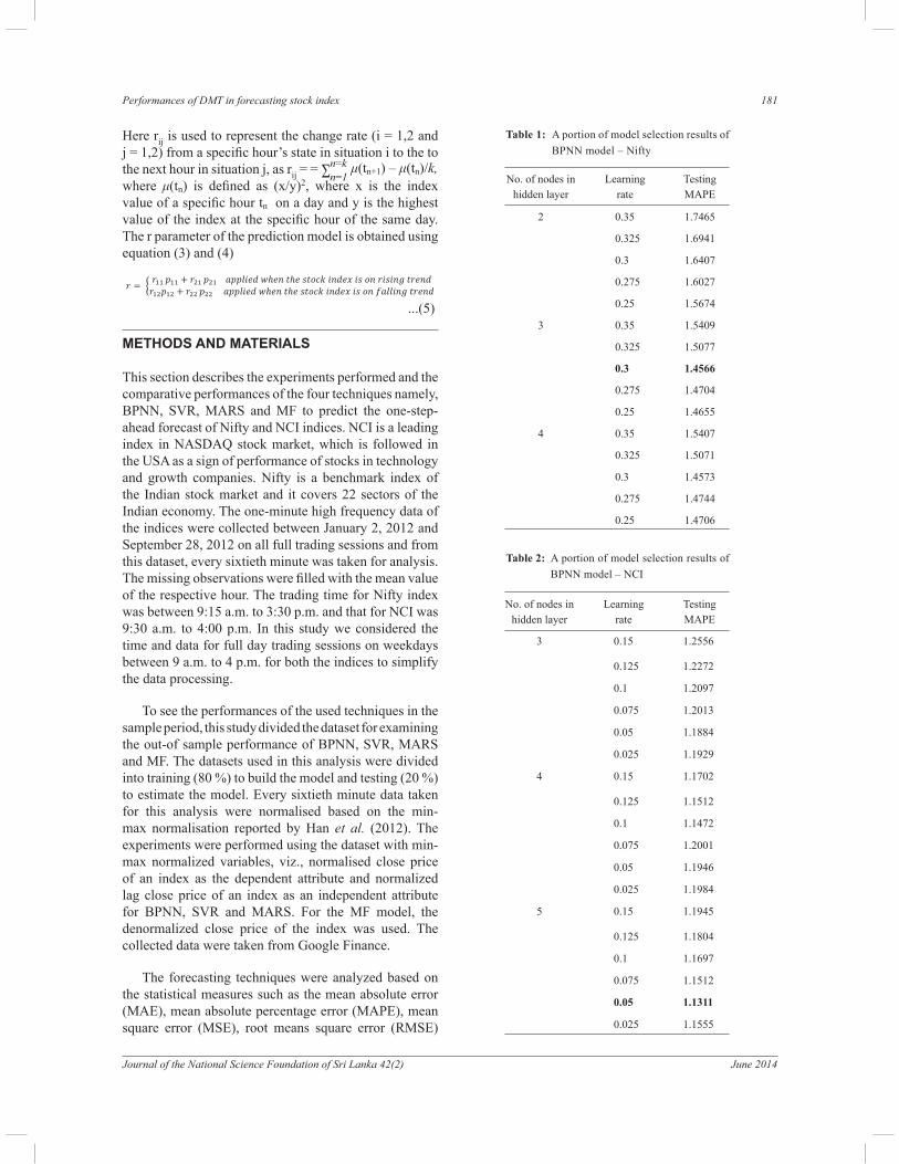
In the representation of BPNN model, the architecture was formed with a single input node in the input layer, three nodes in the hidden layer and a single node in the output layer. The input node consisted of the normalized lagged close price of Nifty or NCI index’s sixtieth minute data as it is the forecasting attribute, and the output node was the the normalized close price as it is the forecasted attribute. The trained BPNN architecture of this study was 1-X-1. This represents the neural network with 1 neuron in the input layer (normalized lagged close price), X neurons in the hidden layer and 1 neuron in the output layer (normalized close price), since one-step ahead prediction is made in this study. Since there are no rules to determine the number of nodes in the hidden layer (Han et al., 2012), the nodes in the hidden

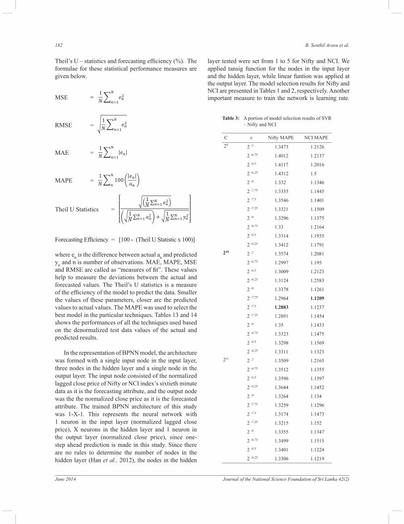
layer tested were set from 1 to 5 for Nifty and NCI. We applied tansig function for the nodes in the input layer and the hidden layer, while linear funtion was applied at the output layer. The model selection results for Nifty and NCI are presented in Tables 1 and 2, respectively. Another important measure to train the network is learning rate.

Table 3: A portion of model selection results of SVR – Nifty and NCI

C ε Nifty MAPE NCI MAPE

29 2 -7 1.3473 1.2126

2 -6.75 1.4012 1.2137

2 -6.5 1.4117 1.2016

2 -6.25 1.4312 1.5

2 -8 1.332 1.1346

2 -7.75 1.3335 1.1445

2 -7.5 1.3546 1.1401

2 -7.25 1.3321 1.1509

2 -9 1.3296 1.1375

2 -8.75 1.33 1.2164

2 -8.5 1.3314 1.1935

2 -8.25 1.3412 1.1791

2102 -7 1.3574 1.2081

2 -6.75 1.2997 1.195

2 -6.5 1.3009 1.2123

2 -6.25 1.3124 1.2583

2 -8 1.3378 1.1261

2 -7.75 1.2964 1.1209

2 -7.5 1.2883 1.1237

2 -7.25 1.2891 1.1454

2 -9 1.35 1.1433

2 -8.75 1.3323 1.1475

2 -8.5 1.3298 1.1569

2 -8.25 1.3311 1.1323

211 2 -7 1.3509 1.2165

2 -6.75 1.3512 1.1355

2 -6.5 1.3596 1.1397

2 -6.25 1.3644 1.1452

2 -8 1.3264 1.134

2 -7.75 1.3259 1.1296

2 -7.5 1.3174 1.1473

2 -7.25 1.3215 1.152

2 -9 1.3355 1.1347

2 -8.75 1.3499 1.1515

2 -8.5 1.3401 1.1224

2 -8.25 1.3306 1.1219



The learning rates with 0.001 to 0.5 were tested in the training process. The number of epochs tested in this study were 10000, 10250, 10500, 10750,...., 25000. To obtain the best parameter in BPNN, the learning rate and the momentum were fine tuned. The BPNN topology with

the minimum testing MAPE was considered as the best.

As the second step, SVR was used to resolve the forecasting problems of BPNN, as it has been proven to be better than BPNN in stock market forecasting. The best SVR model can result only with the selection of best parameters. Hence the RBF kernel was chosen to train the SVR model for this study. Here also fine tuning

was performed to identify the best parameter C and ε for

SVR model with the minimum testing error. The authors have chosen C from 21 to 212 and ε from 2-12 to 212 to identify the best model. Portions of the best out of the combinations are presented in Table 3 for both indices.

Thirdly, the basis functions (BF) were used in the MARS model to forecast the effects of one time lag close of the index on close price of the index. In order to build

the best MARS model, a penalty factor from 1 to 5 was chosen for both time horizons of the indices. The model with the least MAPE from test data was considered as the best model.

For the BPNN and SVR, Weka 3.7.7, developed by Hall et al. (2009) was operated to develop the models. Statistica 10, provided by Statsoft was used in building the MARS models and to develop the MF model Ms Excel 2007 was employed. All the modelling tasks were implemented on an HP Compaq PC with Intel (R) Core (TM) 2 Duo E8400 @ 3.00 GHz CPU processor. The detailed forecasting results of indices using the above mentioned modelling techniques are described in the following section.

RESULTS AND DISCUSSION


Tables 1 and 2 show the testing results of BPNN topology with the combination of different nodes and

Index Variable Basis function

NiftyLag close

BF1 = max(0, Normalized lag close Nifty - 0.243)

BF2 = max(0, 0.243 - Normalized lag close Nifty)

Prediction equation Normalized 60 minute Nifty = 0.243 + 0.993*BF1 -0.977 * BF2

NCILag close

BF1 = max(0, 0.823 - Normalized lag close NCI)

BF2 = max(0, Normalized lag close NCI - 0.803)

BF3 = max(0, Normalized lag close NCI - 0.857)

Prediction equation Normalized 60 minute NCI = 0.8215 - 0.993*BF1 + 0.487 * BF2 + 0.815 * BF3

Table 4: Basis function and prediction equation of MARS – Nifty and NCI

Date TimeClose price µ index

Nifty NCI Nifty NCI

3/1/2012 09:00 4684.65 2657.87 0.968306 0.995941

3/1/2012 10:00 4716.45 2659.56 0.981497 0.997208

3/1/2012 11:00 4719.1 2663.28 0.9826 1

3/1/2012 12:00 4725.55 2653.66 0.985288 0.992789

3/1/2012 13:00 4738.9 2645.94 0.990863 0.987021

3/1/2012 14:00 4728.4 2649.98 0.986477 0.990037

3/1/2012 15:00 4754.05 2655.94 0.997208 0.994496

3/1/2012 16:00 4760.7 2648.72 1 0.989096

Table 5: A portion of stock index data with µ Index – Nifty and NCI



learning rates for Nifty and NCI. From Table 1, it is seen that the minimum MAPE 1.4566 was obtained when 3 nodes were used in the hidden layer. This implies that the Nifty’s every sixtieth minute close price was successfully forecasted by 1-3-1 network topology with a learning rate 0.3 and this network took 15000 iterations to train to produce the lowest MAPE. Hence it is the best network topology in forecasting every sixtieth minute close price of the Nifty index.

From Table 2, it can be observed that the network with 5 nodes in the hidden layer produces the minimum MAPE of 1.1311 for NCI. Furthermore, it is understood that the network with 1-5-1 network topology produces the lowest error with 0.05 as the learning rate and 17500 epochs and hence 1-5-1 network topology is considered as the best in forecasting the NCI index. The forecasting performances of the BPNN topology of each index was analyzed and presented in Table 13 with MSE, RMSE,

MAE, MAPE, Theil U statistic and forecasting efficiency

(%) by denormalizing the normalized predicted data.

Support vector regression

Totally 1152 different SVR models each in Nifty and NCI resulted from the combination of 12 C parameter and 96 ε parameter. A portion of the model selection results is

presented in Table 3 (Nifty and NCI). As observed in Table 3, the combination of C = 210 and ε = 2-7.5 produced the minimum MAPE 1.2883 and was considered the best SVR model for forecasting the Nifty index. From Table 3, it is observed that the minimum MAPE 1.1209 was obtained through the combination of C = 210 and ε = 2-7.75 for forecasting NCI’s every sixtieth minute close price. From this analysis, it is understood that SVR performs better than BPNN in both indices by providing the lowest MAPE. Increasing the C and decreasing the ε parameter

values provided the best results for the indices. The MSE,

Date IndexTime

9:00 10:00 11:00 12:00 13:00 14:00 15:00 16:00

3/1/2012

Nifty 4684.65 4716.45 4719.1 4725.55 4738.9 4728.4 4754.05 4760.7

NCI 2657.87 2659.56 2663.28 2653.66 2645.94 2649.98 2655.94 2648.72

4/1/2012

Nifty 4764.8 4751.45 4756.25 4745.3 4743.05 4779.85 4748.35 4742.15

NCI 2641.66 2635.9 2635.12 2642.64 2649.04 2649.3 2651.19 2648.36

5/1/2012

Nifty 4749.35 4770.85 4767.6 4771.7 4776.85 4761.85 4739.15 4748.7

NCI 2642.19 2636.5 2640.42 2652.55 2662.5 2670.18 2664.43 2669.86

6/1/2012

Nifty 4734 4714 4691.15 4702.05 4703.6 4718.6 4744.95 4760.45

NCI 2669.73 2660.14 2670.09 2678.92 2675.04 2678.87 2678.02 2674.22

Table 6: A portion of stock index data – Nifty and NCI

Date IndexTime

9:00 10:00 11:00 12:00 13:00 14:00 15:00 16:00

3/1/2012 Nifty 1 1 1 1 1 0 1 1

NCI 0 1 1 0 0 1 1 0

4/1/2012 Nifty 1 0 1 0 0 1 0 0

NCI 0 0 0 1 1 1 1 0

5/1/2012 Nifty 1 1 0 1 1 0 0 1

NCI 0 0 1 1 1 1 0 1

6/1/2012 Nifty 0 0 0 1 1 1 1 1

NCI 0 0 1 1 0 1 0 0

Table 7: A portion of stock index rising and falling – Nifty and NCI



RMSE, MAE, MAPE, Theil U statistic and forecasting efficiency (%) of the SVR model of each index are shown

in Table 13 by the denormalized predicted ouput.

Multivariate adaptive regression splines

Here only one variable was considered as the forecasting parameter, and so this variable was automatically selected. In order to explain the MARS prediction model, the first

built Nifty’s MARS model was used as an illustrative example. For example, if the value of normalized lag close Nifty for BF1 = max (0, normalized lag close

Nifty - 0.243) in Table 4 is 0.3, then the BF1 = 0.057 and the model predicts that the normalized close of Nifty is increased by 0.0566 (i.e., 0.993*max (0, 0.3 - 0.243). The obtained basis function and the attribute selection result for Nifty and NCI are presented in Table 4. The out of sample predicted results of the MARS model produced a GCV error of 0.000306 and 0.000310 for Nifty and NCI, respectively. From the results in Table 4, the lowest MAPE obtained for Nifty and NCI, were 1.33062 and 1.523801, respectively. The penalty parameter used to obtain these lowest MAPE was 2 for both indices.

Time

Nifty NCI

p11 p21 p12 p22 p11 p21 p12 p22

9:00 − 10:00 5.5 3.25 5.5 4.25 5.375 4.5 4.75 4

10:00 − 11:00 4.5 4.875 4.25 4.875 5.625 4.625 4.25 4.125

11:00 − 12:00 3.875 4.75 5.5 4.375 5.75 4.75 4.5 3.625

12:00 − 13:00 4.125 4.75 4.5 5.125 6.125 4.125 4.375 4

13:00 − 14:00 4 5.5 4.875 4.125 5.5 4.875 4.75 3.5

14:00 − 15:00 4.625 5.5 4.875 3.5 5.625 3.75 4.75 4.5

15:00 − 16:00 5.5 3.875 4.625 4.5 5 4.625 4.375 4.625

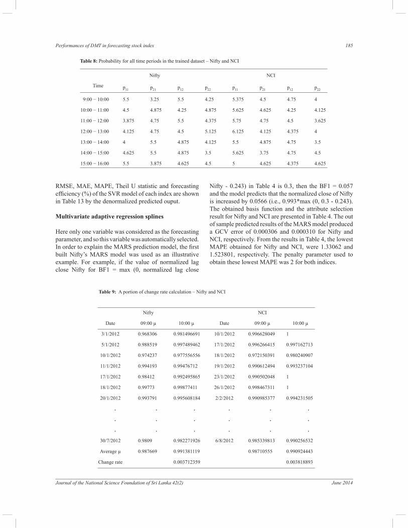
Table 8: Probability for all time periods in the trained dataset – Nifty and NCI

Nifty NCI

Date 09:00 µ 10:00 µ Date 09:00 µ 10:00 µ

3/1/2012 0.968306 0.981496691 10/1/2012 0.996628049 1

5/1/2012 0.988519 0.997489462 17/1/2012 0.996266415 0.997162713

10/1/2012 0.974237 0.977556556 18/1/2012 0.972150391 0.980240907

11/1/2012 0.994193 0.99476712 19/1/2012 0.990612494 0.993237104

17/1/2012 0.98412 0.992495865 23/1/2012 0.990502048 1

18/1/2012 0.99773 0.99877411 26/1/2012 0.998467311 1

20/1/2012 0.993791 0.995608184 2/2/2012 0.990985377 0.994231505

. . . . . .

. . . . . .

. . . . . .

30/7/2012 0.9809 0.982271926 6/8/2012 0.985339813 0.990256532

Average µ 0.987669 0.991381119 0.98710555 0.990924443

Change rate 0.003712359 0.003818893

Table 9: A portion of change rate calculation – Nifty and NCI



Thus, it was found that SVR produced the lowest MAPE compared to the other models. Although MARS model was able of identify the important independent attribute, its forecasting ability for the normalized variables was not as good as those of BPNN and SVR as seen from Tables 1 to 3. In this study the forecasting ability of the models built using these techniques was compared for which the normalized predicted output were denormalized and are presented in Tables 13, and the robustness evaluation on these techniques were analyzed and presented in Table 14.

Markov chain into fuzzy stochastic

Nifty and NCI datasets were used to provide a detailed analysis on the predictive capability of MF. From Table 5, it is observed that the time period considered for this study is reformatted from 9.00 a.m. to 04.00 p.m.

Rising and falling stock index probabilities

The probabilities p11, p12, p21, and p22 in equation (3) and (4) were computed for the rising and falling stock indices from the datasets. To know the value of the index in the next period, we used the mentioned dataset, for example in Table 5 to produce Table 6 for further analysis.

Table 7 indicates the rising and falling measures of the stock index. “0” indicates that the value of the index is falling or equal to the previous state (falling). “1” indicates that the value of the index is rising or equal when compared to the previous state (rising). Now to compute the probabilities p11, p12, p21, and p22 over the training data we use [times of occurrences of (1,1)/ total number of entries] to find p11; [times of occurrences of (0,1)/ total number of entries] to find p12; [times of occurrences of (1,0)/ total number of entries]

Table 10: Stock index change rate for all time periods – Nifty and NCI

Time

Nifty change rate r NCI change rate r

r11 r21 r12 r22 r11 r21 r12 r22

9:00 − 10:00 0.00371 0.00467 - 0.00473 - 0.00485 0.00382 0.00527 - 0.0054 - 0.005

10:00 − 11:00 0.00420 0.00486 - 0.00348 - 0.00324 0.00522 0.00645 - 0.0055 - 0.0063

11:00 − 12:00 0.00306 0.00392 - 0.00511 - 0.0052 0.00335 0.00504 - 0.0052 - 0.0049

12:00 − 13:00 0.00469 0.00448 - 0.00362 - 0.00457 0.00249 0.00361 - 0.0023 - 0.0031

13:00 − 14:00 0.00548 0.00518 - 0.00437 - 0.00659 0.00347 0.00307 - 0.0032 - 0.0035

14:00 − 15:00 0.00550 0.0054 - 0.00642 - 0.00797 0.00253 0.00328 - 0.0029 - 0.0042

15:00 − 16:00 0.00464 0.00522 - 0.00212 - 0.00535 0.00424 0.004543 - 0.0029 - 0.0047

Table 11: Parameter r for the time period 9:00 to 16:00 – Nifty and NCI

Nifty NCI

TimeRising

parameter r

Falling

parameter r

Rising

parameter r

Falling

parameter r

09:00 − 10:00 0.035605 - 0.04662 0.044237 - 0.04551

10:00 − 11:00 0.042577 - 0.03062 0.059392 - 0.04949

11:00 − 12:00 0.030578 - 0.05084 0.043204 - 0.04095

12:00 − 13:00 0.040647 - 0.03971 0.030142 - 0.02246

13:00 − 14:00 0.050364 - 0.04849 0.034056 - 0.02762

14:00 − 15:00 0.055152 - 0.05918 0.026534 - 0.03267

15:00 − 16:00 0.045818 - 0.03387 0.042241 - 0.03442



to find p21 and to find p22 [times of occurrences of (0,0)/ total number of entries]. For example, in Table 7, from timing 9.00 to 10.00, the number of occurrences of (1,1) in Nifty index is 2 and the total number of entries are 8, so p11 is 2/8 = 0.25. In a similar way we can obtain the value for p12, p21 and p22, which is shown in Table 8 for both indices.

Rising and falling change rate

The stock index change rates were calculated for r11, r12, r21, and r22 in equation (5), which are presented in Table 10. For example, in Table 9, a portion of change rate r11 for the time period 9.00 to 10.00 for Nifty index was computed.

Here, we have to calculate the average µ index for the period 9.00 to 10.00 and the change rate by finding

the difference between the average µ index 0.991381119

(10.00) and the average µ index 0.987669 (9.00), and its difference 0.003712359.

Parameter computing and obtaining the predicted

value

Parameter r = r11p11 + r21p21 was used to calculate the rising parameter when the stock value increased, and parameter r = r12p12 + r22p22 was used as a falling parameter for falling stock index values. The computed r parameter values for both indices obtained by combining Table 8 and 10 are presented in Table 11.

The next period index value can be predicted by using the prediction function X(n+1) = X(n)e

r (e represents 2.71828182845904) . For example, to predict the Nifty’s next period value, we have to take the stock index at 9:00, 9:01 and the parameter r. The reformatted stock index at 9:00 (5269.75) and 9:01 (5269.25) on August 6,

Date TimeNifty NCI

Actual Predicted Actual Predicted

7/8/2012 10:00 5309.55 5052.569 3008.58 3140.07

7/8/2012 11:00 5314.8 5540.495 3014.59 2863.301

7/8/2012 12:00 5319.9 5051.338 3024.36 2893.628

7/8/2012 13:00 5327.5 5540.595 3025.29 3116.908

7/8/2012 14:00 5337.3 5602.685 3023.73 2942.865

7/8/2012 15:00 5342.4 5639.931 3021.01 3105.034

7/8/2012 16:00 5331.2 5164.473 3015.86 2918.792

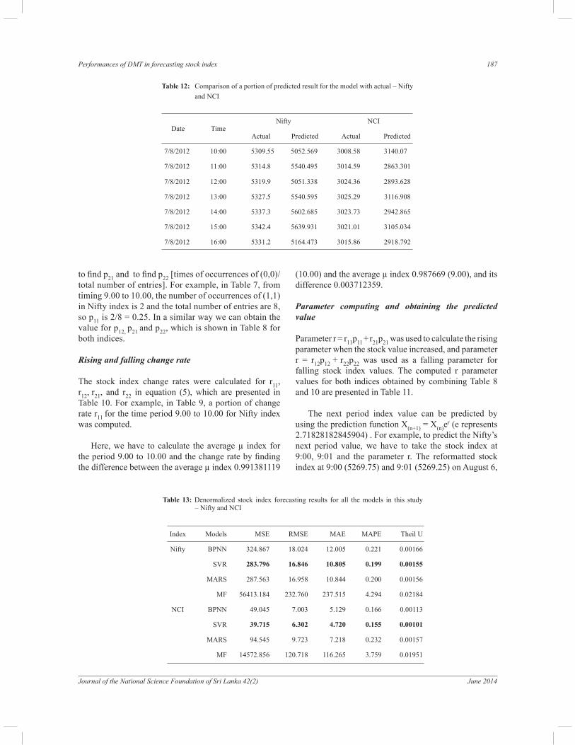
Table 12: Comparison of a portion of predicted result for the model with actual – Nifty

and NCI

Index Models MSE RMSE MAE MAPE Theil U

Nifty BPNN 324.867 18.024 12.005 0.221 0.00166

SVR 283.796 16.846 10.805 0.199 0.00155

MARS 287.563 16.958 10.844 0.200 0.00156

MF 56413.184 232.760 237.515 4.294 0.02184

NCI BPNN 49.045 7.003 5.129 0.166 0.00113

SVR 39.715 6.302 4.720 0.155 0.00101

MARS 94.545 9.723 7.218 0.232 0.00157

MF 14572.856 120.718 116.265 3.759 0.01951

Table 13: Denormalized stock index forecasting results for all the models in this study – Nifty and NCI



Rel

ativ

e ra

tio

Mod

els

Nif

tyN

CI

MS

ER

MS

EM

AE

MA

PE

TH

EIL

UM

SE

RM

SE

MA

EM

AP

ET

heil

U

60 %

BP

NN

301.

228

17.3

5611

.613

0.21

90.

0016

382

.171

9.06

56.

315

0.21

20.

0015

1

SV

R292.1

27

17.0

92

11.3

33

0.2

14

0.0

0161

79.1

71

8.8

98

6.0

00

0.1

95

0.0

0141

MA

RS

293.

208

17.1

2311

.346

0.21

40.

0016

111

3.26

510

.643

7.56

40.

252

0.00

177

MF

3640

6.43

519

0.80

518

7.33

13.

530

0.01

793

7043

.778

83.9

2780

.393

2.68

10.

0139

6

70 %

BP

NN

294.

291

17.1

5511

.521

0.21

50.

0016

074

.214

8.61

55.

944

0.19

70.

0014

2

SV

R274.6

15

16.5

72

11.0

36

0.2

06

0.0

0155

71.1

68

8.4

36

5.7

44

0.1

92

0.0

0140

MA

RS

277.

444

16.6

5711

.071

0.20

70.

0015

611

4.08

110

.681

7.73

90.

254

0.00

176

MF

4533

3.50

621

2.91

720

8.54

33.

901

0.01

986

1092

7.41

610

4.53

410

0.32

93.

305

0.01

718

80 %

BP

NN

324.

867

18.0

2412

.005

0.22

10.

0016

649

.045

7.00

35.

129

0.16

60.

0011

3

SV

R283.7

96

16.8

46

10.8

05

0.1

99

0.0

0155

39.7

15

6.3

02

4.7

20

0.1

55

0.0

0101

MA

RS

287.

563

16.9

5810

.844

0.20

00.

0015

694

.545

9.72

37.

218

0.23

20.

0015

7

MF

5641

3.18

423

2.76

023

7.51

54.

294

0.02

184

1457

2.85

612

0.71

811

6.26

53.

759

0.01

951

90 %

BP

NN

390.

805

19.7

6912

.532

0.22

80.

0018

058

.322

7.63

75.

448

0.17

40.

0012

2

SV

R365.4

1119.1

16

11.7

53

0.2

06

0.0

0170

54.8

65

7.4

07

5.3

78

0.1

69

0.0

011

3

MA

RS

564.

295

23.7

5516

.207

0.29

20.

0021

767

.125

8.19

36.

050

0.19

30.

0013

1

MF

6886

0.31

925

7.24

526

2.41

24.

685

0.02

386

1788

7.97

912

8.84

813

3.74

64.

108

0.02

132

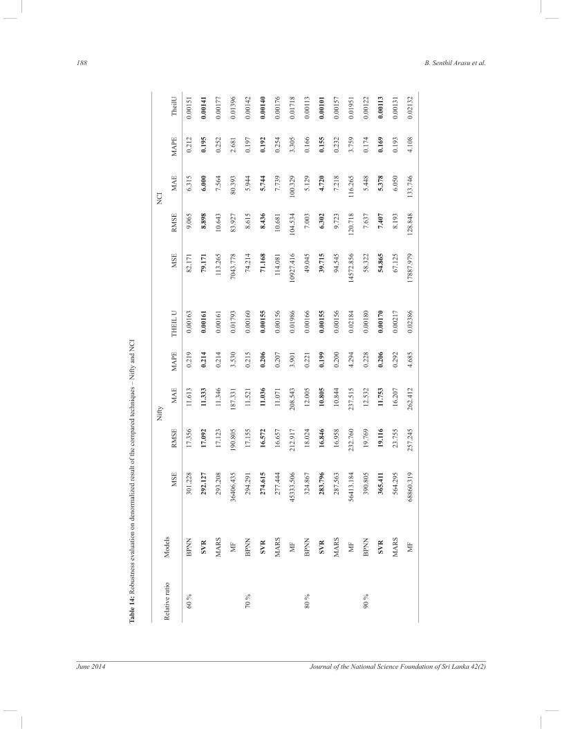
Tab

le 1

4:

Rob

ustn

ess

eval

uati

on o

n de

norm

aliz

ed r

esul

t of

the

com

pare

d te

chni

ques

– N

ifty

and

NC

I



2012, shows that the index is on the falling side and the corresponding falling parameter during 9:00 to 10:00 is -0.04662. Substituting the parameter and the index value at 9:00 in the prediction function 5269.75e-0.04662 gives the predicted value of 5029.71 for the next time period 10.00. Likewise the next hour’s values can be predicted for both indices. A part of the predictions thus made is shown in Table 12.

The performance of MF technique with other compared techniques is presented in Table 13.

Comparative result

Table 13 summarizes the forecasting performances of Nifty and NCI using BPNN, SVR, MARS and MF for the denormalized predicted data. To evaluate the forecasting performance of the best model, MSE, RMSE, MAE, MAPE, Theil U statistic and forecasting efficiency (%)

were used. It can be seen that BPNN, SVR and MARS has a 99.9 % efficiency in forecasting the indices. It is

observed from Table 13 that the forecasting efficiency

of SVR model is 99.99845 % and 99.99899 % in Nifty and NCI, respectively, which was better than the other techniques. From Table 13, we can also observe that MARS outperformed BPNN and MF with lower errors in MSE (287.563), RMSE (16.958), MAE (10.844), MAPE (0.2 %), Theil U statistic (0.00156) and forecasting efficiency (99.99844 %) in forecasting every

sixtieth minute of Nifty. There were smaller deviations between the actual and predicted values when the SVR model was used. Thus the SVR model provided better forecasting results than BPNN, MARS and MF in Nifty and NCI indices.

Robustness evaluation

To evaluate the robustness of the SVR model, the performances of BPNN, MARS and MF models were tested using different ratios of training and testing sample sizes. The experiments were based on the relative ratio of the observations of the training dataset size to the complete dataset size. In this robustness evaluation, we considered four relative ratios: 60 %, 70 %, 80 % and 90 %. Table 14, summarizes the forecasting performaces of the analyzed indices by four techniques in terms of MSE, RMSE, MAE, MAPE and Theil U statistic. The SVR models outperformed the other models in all four different ratios in terms of the five different performance

measures. Thus, the SVR undeniably provides better forecasting results than the other techniques in both Nifty and NCI indices. Based on the discussions and findings

reported in this empirical study, we can say that SVR

model is most suited for forecasting the next period value of the index with higher accuracy when using a single forecasting variable.

CONCLUSION

Earlier studies have examined and compared various sets of data mining techniques in time series forecasting, mostly in the area of ANN, SVC and a series of hybrid models. A sixty-minute dataset from Nifty and NCI indices were used in this study to evaluate the performances of BPNN, SVR, MARS and MF techniques. The use of minute data was found to increase the frequency and fluctuations among the data. MSE, RMSE, MAE,

MAPE, Theil U statistic and forecasting efficiency

(%) were used as performance measures to check the forecasting capability of the techniques. The results shows that an accurate prediction can be made for Nifty and NCI without the use of extensive market related data or macroeconomic variables. SVR models were found to provide better forecasting results than MARS, BPNN and MF in forecasting Nifty and NCI indices. SVR was found to outperform the other techniques in considering the single-time lag close in the input. Also the robustness evaluation for the employed techniques proves that SVR outperforms the other techniques in all the datasets. This study has also justified the recent emergence of

MARS as a better prediction technique for intraday trade than BPNN in Nifty index. It has contributed to the knowledge by evaluating the MARS technique in time series forecasting.

Forecasting stock market is important for fund managers, policymakers, investors, borrowers and traders. This study offers investors and analysts a comparitive study of popular models and recommends the model to use for successful forecasting of stock index.

REFERENCES

1. Abraham A., Steinberg D. & Philip N.S. (2001). Rainfall forecasting using soft computing models and multivariate adaptive regression splines. IEEE SMC Transactions,

Special Issue on Fusion of Soft Computing and Hard

Computing in Industrial Applications 1: 1 − 6.

2. Abreu P.H., Silva D.C., Mendes-Moreira J., Reis L.P. & Garganta J. (2013). Using multivariate adaptive regression splines in the construction of simulated soccer team’s behavior models. International Journal of Computational

Intelligence Systems 6(5): 893 − 910.

3. Balabin R.M. & Lomakina E.I. (2011). Support vector machine regression (SVR/LS-SVM)—an alternative



to neural networks (ANN) for analytical chemistry?

Comparison of nonlinear methods on near infrared (NIR) spectroscopy data. Analyst 136(8): 1703 − 1712.

4. Boorman E.D., Behrens T.E. & Rushworth M.F. (2011). Counterfactual choice and learning in a neural network centered on human lateral frontopolar cortex. PLoS

Biology 9(6): e1001093. DOI: http://dx.doi.org/10.1371/journal.pbio.1001093 5. Butte N.F., Wong W.W., Adolph A.L., Puyau M.R., Vohra

F.A. & Zakeri I.F. (2010). Validation of cross-sectional time series and multivariate adaptive regression splines models for the prediction of energy expenditure in children and adolescents using doubly labeled water. The Journal

of Nutrition 140(8): 1516 − 1523.

6. Cao D.Z., Pang S.L. & Bai Y.H. (2005). Forecasting exchange rate using support vector machines. Proceedings

of IEEE 4th International Conference on Machine Learning

and Cybernetics (ICMLC), volume 6, Guangzhou, China, 18 – 21 August, pp. 3448 − 3452.

7. Chatterjee M. & Majumdar S.K. (2011). Relevance vector machine-based defect modelling and optimisation–an application. International Journal of Operational

Research 12(1): 56 − 78.

8. Chen W.H., Shih J.Y. & Wu S. (2006). Comparison of support-vector machines and back propagation neural networks in forecasting the six major Asian stock markets. International Journal of Electronic Finance 1(1): 49 − 67.

9. Chiang W.C., Urban T.L. & Baldridge G.W. (1996). A neural network approach to mutual fund net asset value forecasting. Omega 24(2): 205 − 215.

10. Dahl G.E., Yu D., Deng L. & Acero A. (2012). Context-dependent pre-trained deep neural networks for large-vocabulary speech recognition. IEEE Transactions on

Audio, Speech, and Language Processing 20(1): 30 − 42.

11. De Andrés J., Lorca P., Cos Juez F.J. & Sánchez-Lasheras F. (2011). Bankruptcy forecasting: a hybrid approach using fuzzy c-means clustering and multivariate adaptive regression splines (MARS). Expert Systems with

Applications 38(3): 1866 − 1875.

12. Demyanyk Y. & Hasan I. (2010). Financial crises and bank failures: a review of prediction methods. Omega 38(5): 315 − 324.

13. Faccio M., Persona A., Pham H. & Regattieri A. (2010). Modelling the spare parts stock levels and its applications in industrial systems. International Journal of Operational

Research 9(1): 39 − 64.

14. Fama E.F. (1991). Efficient capital markets:II. The Journal

of Finance 46(5): 1575 − 1617.

15. Fazel Zarandi M.H., Zarinbal M., Ghanbari N. & Turksen I.B. (2013). A new fuzzy functions model tuned by hybridizing imperialist competitive algorithm and simulated annealing application: stock price prediction. Information Sciences 222: 213 − 228.

16. Friedman J.H. (1991). Multivariate adaptive regression splines. The Annals of Statistics 19(1): 1 − 67.

17. Friston K.J., Jezzard P. & Tuner R. (1994). Analysis of functional MRI time series. Human Brain Mapping 1(2): 153 − 171.

18. Fu T.C. (2011). A review on time series data mining. Engineering Applications of Artificial Intelligence 24(1): 164 − 181.

19. Fu Y. & Cheng Y. (2011). Application of an integrated support vector regression method in prediction of financial

returns. International Journal of Information Engineering

and Electronic Business 3(3): 37 − 43.

20. Hall M., Frank E., Holmes G., Pfahringer B., Reutemann P. & Witten I.H. (2009). The WEKA data mining software: an update. ACM SIGKDD Explorations Newsletter 11(1): 10 − 18.

21. Han J., Kamber M. & Pei J. (2012). Data mining: concepts and techniques, 3rd editon. Elsevier Publishers, San Francisco, USA.

22. José Luis Aznarte M., Alcalá-Fdez J., Arauzo-Azofra A. & Benítez J.M. (2012). Financial time series forecasting with a bio-inspired fuzzy model. Expert Systems with

Applications 39(16): 12302 − 12309.

23. Kao L., Chiu C., Lu C. & Chang C. (2013). A hybrid approach by integrating wavelet-based feature extraction with MARS and SVR for stock index forecasting. Decision

Support Systems 54(3): 1228 − 1244.

24. Kara Y., Acar Boyacioglu M. & Baykan Ö.K. (2011). Predicting direction of stock price index movement using artificial neural networks and support vector machines:

the sample of the Istanbul stock exchange. Expert systems

with Applications 38(5): 5311 − 5319.

25. Kim K.J. (2003). Financial time series forecasting using support vector machines. Neurocomputing 55(1): 307 −

319.26. Kimoto T., Asakawa K., Yoda M. & Takeoka M.

(1990). Stock market prediction system with modular neural networks. Proceedings of the International Joint

Conference on Neural Networks, volume 1, San Diego, USA, 17 – 21 June, pp. 1 − 6.

27. Kumar M. & Thenmozhi M. (2007). Support vector machines approach to predict the S&P CNX NIFTY index returns. 10th Capital Markets Conference, Indian

Institute of Capital Markets. Available at http://ssrn.com/

abstract=962833, Accessed 28 July 2013. DOI: http://dx.doi.org/10.2139/ssrn.962833. 28. Kumar M. & Thenmozhi M. (2012). A hybrid ARIMA–

EGARCH and artificial neural network model in

stock market forecasting: evidence for India and the USA. International Journal of Business and Emerging

Markets 4(2): 160 − 178.

29. Lai R.K., Fan C.Y., Huang W.H. & Chang P.C. (2009). Evolving and clustering fuzzy decision tree for financial

time series data forecasting. Expert Systems with

Applications 36(2): 3761 − 3773.

30. Lee J. & Shin M. (2009). Stock Forecasting using Hidden Markov Processes. cs229 Project

DOI: http://cs229.stanford.adu/proj2009/ShinLee.pdf. 31. Lee T.S. & Chen I.F. (2005). A two-stage hybrid credit

scoring model using artificial neural networks and

multivariate adaptive regression splines. Expert Systems

with Applications 28(4): 743 − 752.

32. Lin C.J., Chen H.F. & Lee T.S. (2011). Forecasting tourism demand using time series, artificial neural networks and



multivariate adaptive regression splines: evidence from Taiwan. International Journal of Business Administration 2(2): 14 − 24.

33. Lu C.J., Chang C.H., Chen C.Y., Chiu C.C. & Lee T.S. (2009). Stock index prediction: a comparison of MARS, BPN and SVR in an emerging market, Proceedings of the

IEEE International Conference on Industrial Engineering

and Engineering Management (ICIEEM), Hong Kong, 8 – 11 December, pp. 2343 − 2347.

34. Lu C.J., Lee T.S. & Lian C.M. (2012). Sales forecasting for computer wholesalers: a comparison of multivariate adaptive regression splines and artificial neural

networks. Decision Support Systems 54(1): 584 − 596.

35. Malkiel B.G. & Fama E.F. (1970). Efficient capital

markets: a review of theory and empirical work. The

Journal of Finance 25(2): 383 − 417.

36. Oh K.J. & Han I. (2000). Using change-point detection to support artificial neural networks for interest rates

forecasting. Expert Systems with Applications 19(2): 105 − 115.

37. Pai P.F. & Lin C.S. (2005). A hybrid ARIMA and support vector machines model in stock price forecasting. Omega 33(6): 497 – 505.

DOI: http://dx.doi.org/10.1016/j.omega.2004.07.024 38. Rathnayake V.S., Premaratne H.L. & Sonnadara D.U.J.

(2011). Performance of neural networks in forecasting short range occurrence of rainfall. Journal of the National

Science Foundation of Sri Lanka 39(3): 251 − 260.

39. Safer A.M. (2003). A comparison of two data mining techniques to predict abnormal stock market returns. Intelligent Data Analysis 7(1): 3 − 13.

40. Sai Y., Yuan Z. & Gao K. (2007). Mining stock market tendency by RS-based support vector machines. Proceedings of the IEEE International Conference

on Granular Computing (ICGC), Silicon Valley, USA, 2 – 4 November, pp. 659.

41. Schierholt K. & Dagli C.H. (1996). Stock market prediction using different neural network classification

architectures. Proceedings of the IEEE/IAFE Conference

on Computational Intelligence for Financial Engineering

(CIFEr), volume 1, Crowne Plaza Manlhattan, New York City, 24 – 26 March, pp. 72 − 78.

42. Smola A.J. & Schölkopf B. (2004). A tutorial on support vector regression. Statistics and Computing 14(3): 199 − 222.

43. Son Y., Noh D.J. & Lee J. (2012). Forecasting trends of high-frequency KOSPI200 index data using learning classifiers. Expert Systems with Applications 39(14): 11607 − 11615.

44. Sureshkumar K.K. & Elango N.M. (2012). Performance analysis of stock price prediction using artificial neural

network. Global Journal of Computer Science and

Technology 12(1): 18 − 25.

45. Tay F.E. & Cao L. (2001). Application of support vector machines in financial time series forecasting. Omega 29(4): 309 − 317.

46. Thenmozhi M. (2006). Forecasting stock index returns using neural networks. Delhi Business Review 7: 59 − 69.

47. Vapnik V. (2000). The Nature of Statistical Learning

Theory, 2nd edition, Springer, New York, USA. DOI: http://dx.doi.org/10.1007/978-1-4757-3264-148. Wang Y.F. (2003). On-demand forecasting of stock

prices using a real-time predictor. IEEE Transactions on Knowledge and Data Engineering 15(4): 1033 − 1037.

49. Wang L. & Zhu J. (2010). Financial market forecasting using a two-step kernel learning method for the support vector regression. Annals of Operations Research 174(1): 103 − 120.

50. Wang Y.F., Cheng S. & Hsu M.H. (2010). Incorporating the Markov chain concept into fuzzy stochastic prediction of stock indexes. Applied Soft Computing 10(2): 613 − 617.

51. Weerasinghe H.D.P., Premaratne H.L. & Sonnadara D.U.J. (2010). Performance of neural networks in forecasting daily precipitation using multiple sources. Journal of

the National Science Foundation of Sri Lanka 38(3): 163 − 170.

52. Wei L.Y., Chen T.L. & Ho T.H. (2011). A hybrid model based on adaptive-network-based fuzzy inference system to forecast Taiwan stock market. Expert Systems with

Applications 38(11): 13625 − 13631.

53. Yao D., Yang J. & Zhan X. (2013). A novel method for disease prediction: hybrid of random forest and multivariate adaptive regression splines. Journal of Computers 08(1): 170 − 177.

54. Zhang D. & Zhang X. (2009). Study on forecasting the stock market trend based on stochastic analysis method. International Journal of Business and

Management 4(6): 163 − 170.

55. Zhang Y. (2004). Prediction of financial time series

with hidden Markov models, M.Sc. thesis, Simon Fraser University, Canada.

56. http://www.google.com/finance/getprices?q=NIFTY&x=

NSE&i=60&p=30d&f=d,o,h,l,c (Nifty - 14 days Backfill

data will be available. Last accessed Aug 20, 2013, 10.30 p.m.).

57. http://www.google.com/finance/getprices?q=.IXIC&x=I

NDEXNASDAQ&i=60&p=30d&f=d,o,h,l,c. (NCI - 14 days Backfill data will be available. Last accessed Aug 20,

2013, 10.30 p.m.).

performances of data mining techniques in forecasting

Documents