performanceevaluationofparametricmodelsinthehindcastingof...

.. -...----- ...- -------------------------------

Indian Journal of Marine SciencesVol. 43(6), June 2014, pp. 899-914

Performance evaluation of parametric models in the hindcasting ofwave parameters along the south coast of Black Sea

Adem Akpinar ':", Mehmet Ozger 2, Serkan Bekiroglu' & Murat Ihsan Komurcu 4

I Uludag University, Civil Engineering Department, 16059 Bursa, Turkey

2 Istanbul University, Civil Engineering Department, 34469 Istanbul, Turkey

3Yildiz Technical University, Civil Engineering Department, 34469 Istonbul, Turkey

4 Karadeniz Technical University, Civil Engineering Department, 61080 Trabzon, Turkey

.[E-mail:[email protected];[email protected]]

Received 11 December 2012; revised 14 January 2013

In the present study, the performances of four parametric models in the wave hindcast were evaluated by comparingwith wave measurements at two locations on the Black Sea, Wilson, SPM, JONSWAP, and CEM methods were used tohindcast significant wave height (H,) and mean wave period (TJ Wind data required to perform wind-wave hindcasts isgathered by the Turkish State Meteorological Service (TSMS) and the European Centre for Medium-Range WeatherForecast (ECMWF), Wave data set measured at deep water location for Hopa and Sinop buoy stations within the NATOTU-WAVES project was used to validate wind-wave hindcasts. A set of new formulations for wind-wave hindcast wasproposed for the Black Sea. Sensitivity analyses were performed for both parametric methods and newly proposed equations,Finally, it is concluded that the CEM method compared to other methods generally produces more accurate results for thehindcasts of wave parameters in both stations, It is observed that parametric methods do not have the sufficiently accurateresults in the Black Sea, Proposed formulations cannot produce results at desired level to represent all southern coasts ofthe Black Sea in comparison to existing parametric methods,

[Keywords: Wave hindcasting, Significant wave height, Wave period, Wave statistics, Parametric methods, Black Sea]

Introduction

Wind waves playa significant role in a variety ofocean and coastal activities including design of coastalstructures, sediment transport, coastal erosion, andpollution transport'. They attack shore protectionstructures, reshape beaches, affect marine structures,and are hence important for commercial, military, andrecreational activities' .. Numerical models solve theenergy balance equation throughout grid points overthe water, where active wave generation is takingplace. These models require abundant bathymetric,meteorological, and oceanographic data. In someregions, these data are not available and numericalmodelling is both difficult and expensive'. Moreover,for first estimates in many cases, the use of thesemodels is not economically justified+ 5.

Several empirical methods such as PM (Piersonand Moskowitz"), Wilson (Wilson7), 5MB(Bretschneider"), JON SWAP (Hasselmann et aI9),

Donelan (Donelan"), SPM (US Army"), and CEM(US Army") have been developed and proposed forthe different seas in the wave hindcast or forecasting.These methods have been often used for variousengineering purposes especially in Turkey and, untiltoday, their performances have been evaluated bysome researchers!'. Bishop" researchedperformances of three manual wave hindcast modelsat two deep-water locations in Lake Ontario. Heexamined only fetch-limited, pseudo-steady-stateevents and found that the accuracy of the Donelanmodel was slightly superior to that of the 5MB andJONSWAP methods. Bishop et al'? compared with

905-9209905-920905-920

Indian Journal of Geo-Marine Sciences

900 INDIAN J MAR SCI VOL 43 (6), JUNE 2014

and Sinop stations in the Black Sea. Finally,development of an appropriate parametric method forthe Black Sea was tried and for this process somescenarios were investigated. The proposed modeldecreased scatter index, but the correlation coefficientwas not enhanced.

Materials and Methods

Study area and the used data

In this study, wave hindcasts were performed fortwo wave measurement stations (Hopa and Sinopbuoys) in the Black Sea. The Black Sea has a laterally-prolonged scale of about 1175 km in the east-westdirection between 28º E and 41.5º E. Its width is about600 km in the north-south direction between 41ºNand 46ºN. This inland sea has an area of 436400kilometer squares (not including the Sea of Azov), amaximum depth of about 2588 m, and a volume of547000 km3 17 Fig. 1 shows the map of the study areaand the locations of the buoy (wave measurementstation) and meteorological stations.

measured wave data and with four wave predictionformulas including SPM, SMB, JONSWAP, andDonelan methods. Their results indicated that SPMmodel tends to overpredict wave height and periodand, statistically, is the poorest predictor of the fourmethods tested. Kazeminezhad et al13 also examinedthe accurate of the CEM method in Lake Ontario forfetch limited condition while Moeini and Etemad-Shahidi16 studied performance of the SPM method inLake Erie. They concluded that the SPM and CEMmethods over-predicted significant wave height whileSPM method under-estimated peak spectral period.Etemad-Shahidi et al5 investigated performances ofthree parametric methods (CEM, SMB, and Wilsonmodels) for predicting the wave height in Ontario andErie lakes. They found that the parametric methodswere more accurate in the fetch limited condition thanin the duration limited condition. The comparison oftheir models also showed that the accuracy of theSMB method was very close to that of the Wilsonmethod while the SMB method was far more accuratethan the CEM method. As can be seen from theliterature, different methods or formulas have beenavailable in different seas or lakes.

The aim of the study is to evaluate the capabilitiesof four different parametric wave models, which havebeen proposed in different coastal and maritimestandards, to reproduce the wave data collected bywave buoys at two positions along the southern coastof the Black Sea. For this purpose, Wilson,JONSWAP, SPM, and CEM methods were appliedto predict wave parameters. In the application of thesemethods, some sensitivity analyses were performedand accuracy of the developed models was determinedand discussed by using buoy measurements at Hopa

Table 1–The characteristics of the buoy and meteorological stations

Station Latitude Longitude

Sinop TSMS station 42o 01' 60" N 35o 09' 60" E

Hopa TSMS station 41o 24' 24" N 41o 25' 58" E

Sinop buoy station and Sinop ECMWF grid point 42o 07' 24" N 35o 05' 12" E

Hopa buoy station and Hopa ECMWF grid point 41o 25' 24" N 41o 23' 00" E

Fig. 1 Location of Study Areas

906

901ADEM et al: PERFORMANCE EVALUATION OF PARAMETRIC MODELS

The wind data required to perform wind-wavehindcasts in this study was obtained from TurkishState Meteorological Services (TSMS) and EuropeanCentre for Medium-Range Weather Forecast(ECMWF). Two coastal wind measurement stationsoperated by TSMS which are the closest stations toHopa and Sinop buoys were selected as a wind datasource. Average of the recorded wind data of theclosest four ECMWF grid points to Hopa and Sinopbuoys was used for wave hindcasting. Thecharacteristics of the buoy and the wind recordingstations are given in Table 1. Both wind data sourceshave advantages and disadvantages. While the TSMSdata have 1 hour time resolution, the ECMWF windfields have a resolution of 6 hours. In other words,while there are 24 pieces of data in 1 day record ofthe TSMS, the data set of the ECMWF has 4 data ina day. However, TSMS data base does not have thespatial resolution. It provides temporal data at several

points along the southern coastline of the Black Sea.On the other hand, the ECMWF data set has spatialresolution of 0.25o and 0.25o in both latitude andlongitude. The used wind data consist of hourlymeasured wind speed and direction for the TSMS,while they are u and v wind components for theECMWF. Joint probability distributions of wind speedand direction for four wind recording stations (fortwo different wind sources at two locations) are givenin Figs. 2 and 3.

The buoy wave data (significant wave height andmean wave period) collected in Hopa and Sinoplocations within the NATO TU-WAVES project whichwas carried out with financial support provided bythe Science for Stability Programme (Phase III) ofNATO was used to validate the wave hindcasts. Whilethe period of the used wind and wave data collectedfor Sinop buoy and meteorological stations includes1994 (November and December months), 1995(November and December months), and 1996 (fromJanuary to June) years, the record period for Hopastations includes whole year of 1995. Water depthsin the buoys are about 100 m and the Hopa buoy isdeployed 4600 m far away from the coast while theSinop buoy was approximately 11600 m off-shore.Statistical summaries of wave and wind data for allstations are presented in Table 2. This table showsthat the observed waves at both buoy stations were

Fig. 2—Spatial variability in DOC and fluorescence indicesin the Sundarban mangroves.

Fig. 3—Spectral characteristics of four fluorophorecomponents identified by the PARAFAC modeling.

907


deep water waves because maximum measured peakperiods at the Hopa and Sinop buoys were 7.404 sand 8.885 s, and thus, the minimum ratio of the waterdepth to the wave length at both stations were 1.17and 0.81, respectively. Moreover, it is understood thatthe average wind and wave directions for Sinop buoyare from the north northwest (NNW) and westnorthwest (WNW) directions, respectively. Besides,it is seen that waves at Hopa buoy often track fromthe west northwest (WNW) direction while windsblow mostly from the southeast (SE) and eastsoutheast (ESE) direction. Joint probabilities(significant wave height & mean wave direction, meanwave period & mean wave direction, significant waveheight & mean wave period) of both buoy locationsare shown in Figures 4, 5, and 6, respectively. Thesejoint probabilities plots for Hopa station represent thedata of whole months of 1995 but they correspondfrom the data of first six months of 1996 and last twomonths of 1994 in Sinop station. Therefore, while

Table 2–Statistics of the recorded wind and wave data during the time period in buoys, ECMWF grid points, andTSMS stations considered in this study

Station Number Parameter Maximum Minimum Averageof data

Sinop buoy 1010 Mean wave direction (derece) 359.957 0.000 204.300

5156 Significant wave height (m) 4.786 0.034 0.601

Mean wave period (s) 8.885 1.889 3.784

Hopa buoy 3552 Mean wave direction (derece) 360.000 0.000 267.842

Significant wave height (m) 4.342 0.068 0.917

Mean wave period (s) 7.404 1.940 3.957

Sinop ECMWF grid 1218 Wind speed (m/s) 12.142 0.230 4.075

point Wind direction (derece) 359.714 0.581 198.962

Sinop TSMS station 1467 Wind speed (m/s) 15.400 1.000 3.944

Wind direction (derece) 360.000 22.500 222.715

Hopa ECMWF grid point 1462 Wind speed (m/s) 8.306 0.050 2.355


Hopa TSMS station 8562 Wind speed (m/s) 11.200 0.000 2.196


908


the joint probability plots for Hopa station representthe characteristics of its wind and wave climate theycan not probably symbolize fully the characteristicsof wind and wave climate of Sinop buoy station.

Hindcasting of wind generated waves

Since the measurement of wind waves is difficultand expensive, most of the time available observationsare very short. Along the Turkish coasts, instrumentalrecording of wave data is not yet systematicallycarried out. There exist only a few wavemeasurements activities in recent years which arerelated to some projects. Wave parameters within theNATO TU-WAVES project which is sponsored byscience for peace unit of NATO were recorded at fewlocations. These measurements are insufficient to betaken into account in the planning phase of a project.Therefore, wave parameters required in planning areestimated from long term wind records18.

Often wind records taken from observations(ships, coastal, offshore structures, buoys, etc.) do notcoincide with the standard 10 m reference level. Theymust be converted to the 10 m reference level topredict the waves. An equation is given to adjust windspeed measured at elevation z to a 10 m height that isappropriate for use in wave hindcast equations. Theelevation adjustment equation is given as 12:

If the data is measured over land it is requiredthat the wind speed (U

land) at 10-m elevation over land

must be converted into the wind speed (Uwater

) at10 m elevation over water. For this purpose, a formulagiven by Hsu [19] is used as:

...(1)

...(2)

Many coastal engineering studies use waveinformation based on the following assumptions:steady wind speed, steady wind direction (thus,constant fetch), and duration of wind long enough toprovide fetch-limited, as opposed to duration-limited,waves14. So, in the hindcast of wave parameters, therequired variables can be determined as wind speed,fetch length, and wind duration20.

Fetch length

Wind fetch length was defined as the unobstructeddistance that wind can travel over water in a constantdirection. In the areas having the coastal irregularitiessuch as inlet, gulf, and embayment, different methodswere described in the literature to take into accountthe effect of the neighboring coasts to fetch length.The most frequently used method is the effectivefetch. The concept of effective fetch assumes that:waves are generated over a 45o range either side ofthe wind direction and energy transfer from wind towaves is proportional to the cosine of the anglebetween the wind and wave directions, and wavegrowth is proportional to fetch length. Hence,

(3)

where Feff

is the effective fetch and is the lengthto be used in the all parametric methods. F

i and Li

i are

fetch lengths and angles measured at 7.5o interval 21, 22.

Wind duration

To determine the duration of winds, definition ofconstant wind was used12. In this way, wind durationat ith hourly data point was considered to be equal tonumber of preceding consecutive and acceptablehours which satisfies following:

iU - U < 2.5 m/s ...(4)

1/7

10 z10

U = Uz

( )0.6water nd

7laU = 3.0 U

2i i

effi

F Cos áF =

Cosá∑

∑

909


oiD - D <15 ...(5)

where and are the average of precedingconsecutive and acceptable hourly wind speed anddirection, respectively. U

i and D

i are the wind speed

and direction at ith hourly data point13.

Parametric wave hindcast methods

The SPM Method

In this method, significant wave height (Hs) and

peak period (Tp) which is the period at the peak of

the wave energy density spectrum are associated withthe wind speed, duration, and fetch length.

( ) ( )s p AH , T f U , F, t= ... (6)

where UA is the wind stress factor (m/s) which is

defined as:

1.23A 10U = 0.71U ... (7)

In the fetch limited case, for the hindcast of wavesfrom wind, SPM method [11] suggested a parametricmodel expressed as:

0.5

s2 2A A

g H g F= 0.0016

U U

... (8)

1/3p

2A A

g T g F= 0.286

U U

... (9)

2/3

min2

A A

g t g F= 68.80

U U

... (10)

where tmin

is minimum wind duration (s) and F isfetch length (m) which was computed as the effectivefetch length in this study. If the wind duration isshorter than the minimum necessary duration to obtainfully developed waves for a certain fetch, the durationlimited case is valid. US Army11 suggests to makeuse of the formulae for the fetch limited case. Itproceeds as: replace t

min by t in Equation 10 and

calculate the equivalent fetch length. Then, calculateH

s and T

p from Equations 8 and 9 where fetch is the

equivalent fetch length23,24 . The relationship between

peak period and mean wave period which is the onlyspectral period that has an equal in the time domainmean period T

z, in the narrow band approximation

equal to Tm02

, is expressed in the following equationfor peak enhancement factor (γ) = 3.321

z pT 0.7775 T≅ ... (11)

The Wilson Method

In this method, the minimum duration for the fullgrowth at a given fetch length is approximatelycalculated by7:

0.73 -0.46min 10t =1.0 F U ...(12)

where U is the wind speed at 10 m above the seasurface (m/s), t

min is in h, and F is in km which was

computed as the effective fetch length in this study.In the fetch limited condition, the significant waveheight (H

s) and period (T

s) are expressed as:

(13)

(14)

If the wind blowing duration is less than tmin

, theassumptions for fetch limited condition become invalid. For this case, equivalent fetch which differsfrom the effective fetch must be calculated. It proceedsas: replace t

min by t in Equation 12 and calculate the

equivalent fetch length. The wave height and periodcan then be estimated by substituting equivalent fetchin the Equations 13 and 145,22.

The significant wave period (Ts) is sometimes

multiplied by a constant to estimate peak period (Tp).

Goda [25] suggested using a value of 1.0515.

s pT 1.05 T≅ ...(15)

The CEM Method

-20.5

s 210

210 g F

HU

=0.30 1- 1+0.004g U

-51/3

1021

s0

U gFT =8.61 1- 1+0.008

g U

910


The minimum wind duration for accomplishing fetchlimited condition is expressed as:

where tmin

is the minimum wind duration (s) and F isfetch length (m) which was computed as the effectivefetch length in this study. In the fetch limited case, thehindcast equations for non dimensional wave height andperiod are:

... (16)

...(17)

...(18)

where is the friction velocity (m/s) estimated as:

...(19)

where is the drag coefficient which is defined as[12]:

...(20)

In duration limited conditions, equivalent fetchlength is calculated as:

...(21)

In this equation, t is the wind duration (s). The equivalentfetch length estimated from this equation must then besubstituted into Equations 17 and 18 to obtain estimates ofwave height and period in duration limited case5,12.

The JONSWAP Spectrum Method

The JONSWAP method predicts parametrically theintegral wave parameters. These parameters are then usedto define the spectrum, using the JONSWAP shape. Thisspectrum is frequently used to describe waves in agrowing phase. The form of the spectrum is defined in

terms of the peak frequency rather than the windspeed as 9

...(22)

where

...(23)

...(24)

...(25)

fp and U are the frequency of spectral peak

and wind speed at 10 m above mean water level.The alpha sets the level of the high frequency tailand the gamma and sigma variables represent thepeak enhancement of the spectral peak of the windsea and the narrowness of this peak, respectively.The mean value of gamma during the JONSWAPexperiment was observed to be 3.3. Significantwave height and zero-crossing wave period aredefined for fetch-limited case as follows:

...(26)

...(27)

and for duration-limited case,

...(28)

...(29)

where Hs, T

z, F, and t are in m, s, km, and h,

respectively. Fetch-limited formulations areappropriate if the following equation is satisfied.

...(30)

Otherwise, equations for duration-limited caseare used 20,26.

1.5-3

2**

g F g t= 5.23 x 10

UU

( )D 10C = 0.001 1.1+ 0.035 U

0.67

min 0.34 0.3310

Ft = 77.23

U g

1/3

2* *

pg T g F= 0.651

U U

( )0.5* 10 DU = U C

( ) ( )2 2 2p p

-4exp - f - f / 2ó f2 -4 -5

p

5 fE f = á g (2ð) f exp -

4 f

γ

( ) 0.2220.076 g F U−−α =

( ) 0.332

p

3.5 g g F Uf

U

−−

=

0.07

0.09

< = ≥

p

p

f fó

f f

0.5

-2s2 2* *

g H g F= 4.13 x 10

U U

1/2sH = 0.0163F U

3/10 2/5zT = 0.439 F U

5/7 9/7sH = 0.0146 t U

3/7 4/7zT = 0.419 t U

0.7 0.4t >1.167 F / U

911


Application of the parametric methods to theBlack Sea

Four different parametric methods mentionedabove sections were applied to the Black Sea usingthe ECMWF and TSMS wind data. Eight differentmodel combinations for two wave parameters(significant wave height and mean wave period) inboth stations (Hopa and Sinop stations) wereseparately constituted (Tables 3 and 4). Waveparameters (H

s and T

z) were estimated using wind

data and parametric models, which were consideredfor Hopa and Sinop stations. For this process, windspeed and direction at 10 m elevation over the sealevel in Hopa and Sinop stations were firstlydetermined for the TSMS wind data source by usingEquations 1 and 2. Also, resultant wind velocity anddirection in both stations for the ECMWF data setwere calculated from wind components. The fetchlengths for all wind directions recorded at the stations

in the ECMWF and TSMS data bases weredetermined as the effective fetch from Equation 3.Wind durations which are equal to number ofconsecutive hours were obtained from wind recordsas stated in section 3.2. Corresponding wind speedsand fetch lengths are also determined by taking theirmean values over this duration (see Bishop 14 andÖzger and sen20). Finally, wave hindcasts wereperformed from the time series of both data sourcesfor two stations, and then, wave parameters werehindcasted by using two wind sources at Hopa andSinop stations.

Buoy data used in this study has not regulartemporal resolution and there are gaps in the records.On the other hand, wave hindcasts are performed fromwind records with a certain temporal resolution. So,occurrence times of the hindcast data do not coincidewith that of buoy data. In order to determine thestatistical error indices, hindcast data must be

Table 3—Error statistics of parametric methods in the hindcasts of wave parameters for Hopa station

Data sources - The number of Bias SI RMSE MAE R R2

Hindcast method concurrent data parameter

Significant wave height (Hs, m)

TSMS – JONSWAP 1083 -0.500 1.212 0.782 0.516 0.295 0.087

TSMS – CEM (12 months) -0.525 1.240 0.801 0.535 0.279 0.078

TSMS – SPM -0.473 1.177 0.760 0.503 0.322 0.104

TSMS – Wilson -0.489 1.180 0.762 0.501 0.389 0.151

ECMWF –JONSWAP 690 -0.401 1.188 0.640 0.424 0.322 0.104

ECMWF – CEM (12 months) -0.421 1.212 0.653 0.435 0.322 0.104

ECMWF – SPM -0.395 1.178 0.634 0.424 0.334 0.112

ECMWF - Wilson -0.451 1.246 0.670 0.454 0.399 0.159

Mean wave period (Tz, s)

TSMS – JONSWAP 1083 -2.486 0.735 2.847 2.533 0.014 0.000

TSMS – CEM (12 months) -3.000 0.832 3.223 3.000 0.021 0.000

TSMS – SPM -2.513 0.733 2.840 2.538 0.033 0.001

TSMS – Wilson -2.866 0.798 3.092 2.866 0.079 0.006

ECMWF –JONSWAP 690 -2.115 0.708 2.650 2.332 0.114 0.013

ECMWF – CEM (12 months) -2.755 0.803 3.007 2.760 0.120 0.014

ECMWF – SPM -2.308 0.721 2.701 2.388 0.124 0.015

ECMWF - Wilson -2.940 0.839 3.144 2.940 0.163 0.026

912


simultaneous with the buoy data. Therefore, buoy dataand hindcasts are coupled.

For quantitative evaluation of the models,simultaneous buoy data and hindcasts were comparedwith each other. The error statistics of significant waveheight and mean wave period predicted by parametricmethods for Hopa and Sinop stations are presentedin Tables 3 and 4. The scatter index (SI), biasparameter, root mean square error (RMSE), meanabsolute error (MAE), correlation coefficient (R), anddetermination coefficient (R2) were used to evaluatethe degree of accuracy of the results. These statisticalparameters were calculated as follows:

...(31)

...(32)

...(33)

...(34)

...(35)

where Oi is the observed value, O is the mean

value of the observed data, Pi is the predicted value,

Table 4—Error statistics of parametric methods in the hindcasts of wave parameters for Sinop station

Data sources - The number of Bias SI RMSE MAE R R2

Hindcast method concurrent data parameter

Significant wave height (Hs, m)

TSMS – JONSWAP 461(10 months) -0.491 0.903 0.991 0.704 0.285 0.081

TSMS – CEM -0.550 0.937 1.023 0.742 0.272 0.074

TSMS – SPM -0.263 0.962 1.056 0.718 0.317 0.100

TSMS – Wilson -0.479 0.837 0.919 0.645 0.370 0.137

ECMWF – JONSWAP 426(10 months) -0.496 1.054 0.956 0.580 0.304 0.092

ECMWF – CEM -0.552 1.072 0.973 0.605 0.335 0.112

ECMWF – SPM -0.409 1.048 0.951 0.575 0.293 0.086

ECMWF - Wilson -0.625 1.125 1.021 0.650 0.308 0.095

Mean wave period (Tz, s)

TSMS – JONSWAP 461(10 months) -0.842 0.562 2.289 1.881 0.111 0.012

TSMS – CEM -2.202 0.626 2.549 2.307 0.106 0.011

TSMS – SPM -1.055 0.505 2.055 1.760 0.133 0.018

TSMS – Wilson -2.006 0.568 2.313 2.068 0.193 0.037

ECMWF – JONSWAP 426(10 months) -0.769 0.534 2.085 1.721 0.070 0.005

ECMWF – CEM -2.112 0.618 2.409 2.157 0.085 0.007

ECMWF – SPM -1.135 0.516 2.014 1.643 0.079 0.006

ECMWF - Wilson -2.406 0.673 2.626 2.411 0.078 0.006

( )N

i ii 1

1bias = P - O

N=∑

N

ii = 1

RMSESI =

1O

N∑

( )N 2

i ii =1

1RMSE = P-O

N∑

N

i ii = 1

1MAE = P - O

N∑

( )( )( )( ) ( )

N

i ii 1

N N2 2

i ii 1 i 1

P - P O - OR =

P - P O - O

=

= =

∑

∑ ∑

913


P is the mean value of the predicted data, and N isthe number of data.

The performances of eight model combinationsin the estimations of significant wave height and meanwave period can be seen in Tables 3 and 4. Althoughthe results show that Wilson method is more accuratethan other parametric methods and accuracy of themodels is not in the desired level because R2 and SIvalues of the hindcasts are much lower than 0.5 value.The possible reasons may be the measurement errors,unsuitability of parametric methods for the Black Sea,and the errors in determining the wind blowingduration. Besides, the source of the errors may alsobe the wind speed itself. Considering the buoylocations, the dominant wind direction, and theresolution of the atmospheric model, it is seen thatwinds blowing from land are strongly affected by landeffects.

Since the parametric methods did not producedsatisfactory results, it is decided to perform analysesfor various values of the most appropriate criticalangle of wind direction change which plays a limitingrole in the determination of wind blowing duration.In the next section, a sensitivity analysis was carriedout to determine the most appropriate value for theangle of direction change.

Sensitivity analysis for determination of the windduration

In wave hindcast methods, there are two criteriathat control the procedure in the determining the windblowing duration. The first one is the amount ofchange in the wind direction. It is assumed that thestorm continues if the change in wind direction is lessthan a presumed value such as 15o, 30o, 45o, 90o etc.otherwise storms ends and a new storm starts. Thetime between the start and end of the storm is acceptedas the wind duration. The second one is the amountof change in wind speed. If the change in wind speedis less than a given value (such as 2.5 m/s) then thismeans that storm continues 27. When the wind recordsare examined (Figure 7), it is seen that while thechange in wind speed is very low, the change in wind

direction is significant. In other words, it is sensitivein determining of wind blowing duration. Therefore,it was decided to use wind direction as a selectionrule in determining of wind duration. The mostappropriate angle of wind direction change wassearched for Hopa and Sinop stations, and for bothwind data sources by comparing the measured andhindcasted data obtained by considering differentangles of wind direction change.

In this study, to determine the wind duration, eightdifferent values 15o, 30o, 45o, 60o, 75o, 90o, 105o, and120o as the value of the critical wind direction changeangle were investigated. Wind durations weredetermined separately for all angles of directionchange from the time series of the ECMWF andTSMS data recorded at Hopa and Sinop stations.Afterwards, corresponding wind speeds and directionsand fetch lengths are also determined by taking theirmean values over these durations. The JONSWAPmethod that is the most widely used parametric wavehindcast method was selected to make estimations ofwave characteristics. Wave hindcasts were performed

914


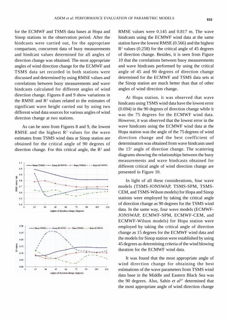
for the ECMWF and TSMS data bases at Hopa andSinop stations in the observation period. After thehindcasts were carried out, for the appropriatecomparison, concurrent data of buoy measurementsand hindcast values determined for all angles ofdirection change was obtained. The most appropriateangles of wind direction change for the ECMWF andTSMS data set recorded in both stations werediscussed and determined by using RMSE values andcorrelations between buoy measurements and wavehindcasts calculated for different angles of winddirection change. Figures 8 and 9 show variations inthe RMSE and R2 values related to the estimates ofsignificant wave height carried out by using twodifferent wind data sources for various angles of winddirection change at two stations.

As can be seen from Figures 8 and 9, the lowestRMSE and the highest R2 values for the waveestimates from TSMS wind data at Sinop station areobtained for the critical angle of 90 degrees ofdirection change. For this critical angle, the R2 and

RMSE values were 0.145 and 0.817 m. The wavehindcasts using the ECMWF wind data at the samestation have the lowest RMSE (0.566) and the highestR2 values (0.258) for the critical angle of 45 degreesof direction change. Besides, it is seen from Figure10 that the correlations between buoy measurementsand wave hindcasts performed by using the criticalangle of 45 and 90 degrees of direction changedetermined for the ECMWF and TSMS data sets atthe Sinop station are much better than that of otherangles of wind direction change.

At Hopa station, it was observed that wavehindcasts using TSMS wind data have the lowest error(0.694) in the 90 degrees of direction change while itwas the 75 degrees for the ECMWF wind data.However, it was observed that the lowest error in thewave hindcasts using the ECMWF wind data at theHopa station was the angle of the 75 degrees of winddirection change and the best coefficient ofdetermination was obtained from wave hindcasts usedthe 15o angle of direction change. The scatteringdiagrams showing the relationships between the buoymeasurements and wave hindcasts obtained fordifferent critical angle of wind direction change arepresented in Figure 10.

In light of all these considerations, four wavemodels (TSMS-JONSWAP, TSMS-SPM, TSMS-CEM, and TSMS-Wilson models) for Hopa and Sinopstations were employed by taking the critical angleof direction change as 90 degrees for the TSMS winddata. In the same way, four wave models (ECMWF-JONSWAP, ECMWF-SPM, ECMWF-CEM, andECMWF-Wilson models) for Hopa station wereemployed by taking the critical angle of directionchange as 15 degrees for the ECMWF wind data andthe models for Sinop station were established by using45 degrees as determining criteria of the wind blowingduration for the ECMWF wind data.

It was found that the most appropriate angle ofwind direction change for obtaining the bestestimations of the wave parameters from TSMS winddata base in the Middle and Eastern Black Sea wasthe 90 degrees. Also, Sahin et al27 determined thatthe most appropriate angle of wind direction change

915


to obtain the best wave hindcast results from theTSMS data in the Western Black Sea was the 90degrees28.

Results and Discussions

Performance evaluation of parametric methods in theBlack Sea

The critical angle for wind direction change wasdetermined for each station using sensitivity analysisin the implementation of parametric methods. Byconsidering this critical angles wave hindcasts werecarried out using ECMWF and TSMS wind data atHopa and Sinop stations. Predicted and observedwave parameters were compared to each other. Tables5 and 6 present the error statistics for concurrenthindcasts and buoy measurements at Hopa and Sinopstations. As can be seen from these tables, the modelsusing the ECMWF wind source have lower RMSEvalues and correlation coefficients than the modelsusing the TSMS wind data for hindcasts of significantwave height at Hopa station. In contrast to this, inhindcasts of mean wave period for the same station,it was observed that the models using the ECMWFwind source have higher RMSE values and correlationcoefficients than the models using the TSMS winddata. At Sinop station, it is seen that RMSE values ofthe models using the ECMWF wind source are lowerthan that of the models using the TSMS wind datafor both wave parameters. But, while correlationcoefficients of the models using the ECMWF windsource are higher than that of the models using theTSMS wind data for significant wave height, it islower for mean wave period. Also, it is understoodthat the SPM method using the ECMWF wind datahas better results (RMSE=0.634 m and R=0.334) forhindcasts of significant wave height whileperformance of the CEM method using the TSMSwind data is better (RMSE=2.038 s and R=0.047) thanthat of the other methods for mean wave period atHopa station. Also, It is observed for Sinop stationthat the CEM method using the ECMWF wind datahas better results (RMSE=0.533 m and R=0.563 forH

s and RMSE=1.478 s and R=0.048 for T

z) for

hindcasts of both wave parameters. Besides, it canbe say that error and correlation values of all models

are close to each other. Therefore, time series ofhindcasts of H

s and T

z from parametric methods were

also discussed. A comparison of time series ofhindcasts of H

s and T

z from parametric methods with

buoy data for two stations is also illustrated in Figures11 and 12. As can be seen from this figures, theJonswap and Wilson methods has low hindcasts ofwave parameters while the SPM method has generallyhindcasts close to buoy data. Also, it is observed fromthese figures that the CEM method compared to othermethods mostly produces more accurate results in thehindcasts of wave parameters for both wind sourcesin both stations. Storms in time series of waveparameters measured in buoy stations were observedin the model estimations. In addition to, the results ofthe models using the ECMWF wind source at Hopastation are significantly low. However, at Sinopstation, this situation is not seen. This may be due toorography effects. .

Proposed models for the Black Sea

Performance evaluations of the classical wavehindcast methods for the Black Sea show thatparametric wave hindcast models are not in the desiredlevel of accuracy (because R values of the hindcastsare lower than 0.7 value) for the study area. The bestwave hindcast method developed has very low R2

values (max. R2=0.195 for Hs and 0.026 for T

z at Hopa

station and 0.331 for Hs and 0.040 for T

z at Sinop

station) and higher errors (min. RMSE=0.634 m forH

s and 2.038 s for T

z at Hopa station and 0.533 m for

Hs and 1.478 s for T

z at Sinop station) as can be seen

from Tables 5 and 6. Therefore, in this part of thestudy, new models which can represent the waveconditions in the southern coasts of the Black Seawith higher correlation coefficient and lower errorcompared to the classical wave hindcast methods wereproposed to predict the wave parameters. For thispurpose, different combinations were studied asfollows:

Ø The constants found in the equations of theclassical methods were re-determined by usingmeasured data for Hopa and Sinop stations. Forinstance, the JONSWAP method was consideredas follows for fetch- and duration-limited cases:

916


Table 5—Error statistics of concurrent data of hindcasted wave parameters with the buoy measurementsat Hopa station

Data source – Critical angle of Significant wave height Mean wave periodHindcast method direction change (H

s, m) (T

z, s)

(degrees)

RMSE value R RMSE value R

TSMS – JONSWAP 90 0.694 0.327 2.511 0.033

TSMS – CEM 0.744 0.419 2.038 0.047

TSMS – SPM 0.880 0.439 2.504 0.027

TSMS – Wilson 0.684 0.442 2.824 0.078

ECMWF – JONSWAP 15 0.640 0.322 2.650 0.114

ECMWF – CEM 0.653 0.322 3.007 0.120

ECMWF – SPM 0.634 0.334 2.701 0.124

ECMWF - Wilson 0.670 0.399 3.144 0.163

Table 6—Error statistics of concurrent data of hindcasted wave parameters with the buoy measurements at Sinop station

Data source – Critical angle of Significant wave height Mean wave period Hindcast method direction change (H

s, m) (T

z, s)

(degrees) RMSE value R RMSE value R

TSMS – JONSWAP 90 0.817 0.380 2.457 0.091

TSMS – CEM 1.040 0.500 1.624 0.175

TSMS – SPM 1.382 0.466 2.550 0.202

TSMS – Wilson 0.756 0.425 2.593 0.123

ECMWF – JONSWAP 45 0.566 0.508 2.144 0.016

ECMWF – CEM 0.533 0.563 1.478 0.048

ECMWF – SPM 0.589 0.576 1.778 0.066

ECMWF - Wilson 0.655 0.552 2.500 0.053

where a, b, c, d, e, and f constants were optimizedbased on the measured data of both stations. Theconstants of above equations were re-determined byusing the ECMWF wind source at Hopa station. But,correlation coefficient of the developed model wasnot enhanced by comparison the existing Jonswapequations. The developed model had R=0.30 butcorrelation coefficient of Jonswap method was 0.32.Besides, the performance of the developed model forthe fetch and duration limited cases was investigated.

Correlation coefficients for fetch and duration limitedcases were 0.11 and 0.30, respectively. From this, itwas understood that the developed model has greaterrors for fetch limited condition compared to durationlimited case. This may be due to 45o range used forthe concept of effective fetch. Then, the performanceof the developed model was discussed for other windsource (TSMS) and other station (Sinop). It was foundthat the developed model has worse performance thanthe Jonswap method for both cases.

917


Ø The constants of the equation used for tmin

calculation in the JONSWAP method were alsodetermined by assigning different values todevelop equations having lower errors and highercorrelation coefficients for both stations.However, no improvement was achieved.

From the results of above two steps, it is shownthat more the proposed models can not produce moreaccurate wave hindcasts than existing methods.

Ø Since the results from first two steps are not atdesired level. Different functions such as weibull,fourier, gauss, polynomial, sinus, exponential,and power type functions were fitted using linearand nonlinear least squares techniques. Thegenerated equations were applied to the otherstation to obtain a general equation being validfor both stations. It is seen that the fitted modelshave better performances compared toparametric wave hindcast models at the stationwhich its data is used for calibration. However,same model gives worse results at other station.

Ø Curve fitting was also performed by usingdifferent x and y variables (for example y = H/Uand x = t for duration-limited condition and y =H and x = F/U for fetch-limited condition). Theresults can not be improved so much. Similarresults were obtained with abovementionedregression models.

Ø The scenarios mentioned above steps wererepeated for the dataset covering the all data oftwo stations. However, no improvement wasachieved.

Ø Finally, average and standard deviation of datawere calculated for each station. Curve fittingwas performed by using the remaining data inthe band created by adding and subtractingstandard deviation from the average value. Thepurpose of this pre-processing is to createsmoother curves. Results of equations generatedin this way have not been achieved efficiently torepresent all southern coasts of the Black Sea bycomparison the existing parametric methods.

It is concluded that while the proposed modeldecreased scatter index, but the correlation coefficientwas not enhanced. These results show that applicationof such simplified methods or parametric models doesnot improve model performance along the southcoasts of the Black Sea. Third-generation wavemodels like SWAN model29 are systematically usedworld-wide both for research and engineeringapplications with extremely accurate results. On theother hand, it is well recognized that third generationswave models perform extremely well provided thewind fields are accurate enough. Therefore,academicians and engineers interested in the studyarea should tend to implementation of these modelsrather than application of simplified methods foractivities in this area.

Conclusions

In this study, the accuracy of the parametric wavehindcast methods such as Wilson, SPM, JONSWAP,and CEM models was investigated by using twodifferent wind sources at two locations in the BlackSea. Totally 32 different parametric wave models weretried for both significant wave height and mean waveperiod hindcast. Results reveal that Wilson methodis the most accurate model compared to otherparametric methods for the initial analysis. It is alsoseen that parametric wave models are not at thedesired level of accuracy for wave parametershindcast.. In the light of determined critical angles ofwind direction change for each station and windsource, it is found that the CEM method compared toother methods generally produces more accurateresults in the hindcasts of wave parameters in bothstations. Hindcasts of significant wave height arebetter than that of mean wave period in terms ofcorrelation coefficients. The newly proposed modeldecreased scatter index, but the correlation coefficientwas not enhanced and the desired level of accuracywas not obtained. CEM method can be used inextremely simple practical applications. It issuggested to academicians and engineers working inthe field of interest of this study that they should tendto implementation of developed numerical models(e.g. third generation wave models – SWAN) rather

918


than application of parametric methods for importantcoastal engineering design activities in this area.

Acknowledgements

Authors would like to thank the ECMWF forproviding its wind forcing data and the TSMS forproviding its wind data and for its helps in recruitingthe necessary permissions for obtaining data from theECMWF. Authors acknowledge Prof. Dr. ErdalÖzhan of the Middle East Technical University,Ankara, Turkey, who was the Director of the NATOTU-WAVES, for providing the buoy data, and theNATO Science for Stability Program for supportingthe NATO TU-WAVES project. This study is aproduct of the PhD thesis of Adem Akpinar.

References

1 Moeini, M.H., Etemad-Shahidi, A., Application of twonumerical models for wave hindcasting in Lake Erie,Applied Ocean Research, 29 (2007) 137-145.

2 Kazeminezhad, M.H., Etemad-Shahidi, A., Mousavi, S.J.,Evaluation of neuro fuzzy and numerical wave predictionmodels in Lake Ontario, Journal of Coastal Research,Special Issue, 50 (2007) 317-321.

3 Browne, M., Castelle, B., Strauss, D., Tomlinson, R.,Blumenstein, M., Lane, C., Near-shore swell estimationfrom a global wind-wave model: spectral process, linear,and artificial neural network models. Coastal Engineering,54 (2007) 445-460.

4 Goda, Y., Revisiting Wilson’s formulas for simplified wind-wave prediction. Journal of Waterway, Port, Coastal andOcean Engineering, ASCE, 129 (2003) 93-95.

5 Etemad-Shahidi, A., Kazeminezhad, M.H., Mousavi, S.J.,On the prediction of wave parameters using simplifiedmethods, Journal of Coastal Research, Special Issue, 56(2009) 505-509.

6 Pierson, W.J., Moskowitz, L., A proposed spectral formfor fully developed seas based on the similarity theory ofS.A. Kitaigorodskii. Journal of Geophysical Research, 69(1964) 5181–5191.

7 Wilson, B.W., Numerical prediction of ocean waves in theNorth Atlantic for December, 1959, Ocean Dynamics, 18(1965) 114-130.

8 Bretschneider, C.L., Wave forecasting relations for wavegeneration. Look Lab, Hawaii, 1 (3), 1970.

9 Hasselmann, K., Barnett, T.P., Bouws, E., Carlson, H.,Cartwright, D.E., Enke, K., Ewing, J.A., Gienapp, H.,Hasselmann, D.E., Kruseman, P., Meerburg, A., Mller, P.,Olbers, D.J., Richter, K., Sell, W., Walden, H.,

Measurements of wind-wave growth and swell decayduring the joint North Sea wave project (JONSWAP).Ergnzungsheftzur Deutschen Hydrographischen ZeitschriftReihe, Deutsches Hydrographisches Institute, Hamburg,Germany, 1973.

10 Donelan, M.A., Similarity theory applied to the forecastingof wave heights, periods and directions, paper presentedat the Canadian Coastal Conference (Canada), pp. 47-61,1980.

11 U.S. Army, Shore Protection Manual, U.S. Army EngineerWaterways Experiment Station, U.S. Government PrintingOffice, Fourth Edition – No. 20402, Washington (DC),USA, 1984.

12 U.S. Army, Coastal Engineering Manual, Chapter II-2,Meteorology and Wave Climate, U.S. Army EngineerWaterways Experiment Station, U.S. Government PrintingOffice, No. EM 1110-2-1100, Washington (DC), USA,2003.

13 Kazeminezhad, M.H., Etemad-Shahidi, A., Mousavi, S.J.,Application of fuzzy inference system in the prediction ofwave parameters, Ocean Engineering, 32 (2005) 1709-1725.

14 Bishop, C.T., Comparison of manual wave predictionmodels. Journal of Waterway, Port, Coastal and OceanEngineering, ASCE, 109 (1983) 1-17.

15 Bishop, C.T., Donelan, M.A., Kahma, K.K., Shoreprotection manual’s wave prediction reviewed. CoastalEngineering, 17 (1992) 25-48.

16 Moeini, M.H., Etemad-Shahidi, A., Evaluation of SWANnumerical model & SPM method for wave hindcasting,paper presented at the 7th International Conference oncoasts, ports and marine structures (Tehran, Iran), pp. 416-422, 2006.

17 Akpinar, A., Kömürcü, M.I., Özger, M., Kankal, M., Theapplication of SWAN for wave simulation in Black Sea,paper presented at the 7th National Coastal EngineeringConference (Trabzon, Turkey), pp. 269-280, 2011 (inTurkish).

18 Ergin, A., Coastal Engineering, Ankara, Turkey: METUPress, No. 9789944344821, 392p, 2009.

19 Hsu, S.A., On the correction of land-based windmeasurements for oceanographic applications, paperpresented at the 17th International Conference on CoastalEngineering -ASCE (Sydney, Australia), pp. 708-724,1980.

20 Özger, M., Sen, Z., Triple diagram method for theprediction of wave height and period. Technical Notes.Ocean Engineering, 34 (2007) 1060-1068.

21 Reeve, D., Chadwick, A., Fleming C., Coastal Engineering:Processes, theory, and design practice. Spon Press, Taylorand Francis Group, London and New York, 2004.

919


22 Yüksel, Y., Çevik, E.Ö., Coastal Engineering. Istanbul,Turkey: Beta Publishing Inc., Marine Engineering Series–No. 1, 732p, 2009 (in Turkish).

23 Ozeren, Y., Wren, D.G., Predicting wind-driven waves insmall reservoirs, Technical Note, Trans. ASABE, 52 (2009)1213-1221.

24 Liu, Z., Frigaard, P., Generation and analysis of randomwaves, Laboratoriet for Hydraulik og Havnebygning,Instituttet for Vand, Jord og Miljoteknik, AalborgUniversitet, Denmark, 2001.

25 Goda, Y., Random seas and design of maritime structures.University of Tokyo Press, 323p, 1985.

26 Özger, M., Wave energy prediction and stochastic

modeling. Ph.D. Thesis, Istanbul Technical University,Istanbul, Turkey, 2007 (in Turkish).

27 Sahin, C., Aydogan, B., Çevik, E., Yüksel Y., Parametricwave modeling with wave data of south-west Black Sea,paper presented at the VI. National Coastal EngineeringConference (Izmir, Turkey), pp. 249-256, 2007 (inTurkish).

28 Akpinar, A., Wave modeling and wave energy potentialdetermination in the Black Sea. Ph.D. Thesis, KaradenizTechnical University, Trabzon, Turkey, 2012 (in Turkish).

29 Booij, N., Holthuijsen, L.H., Ris, R.C., A third-generationwave model for coastal regions. 1. Model description andvalidation, Journal of Geophysical Research, 104 (1999)

7649-7666.

920

performanceevaluationofparametricmodelsinthehindcastingof...

Documents