performance pay and the autocovariance structure of

Performance Pay and the Autocovariance Structure of

Earnings and Hours�

Thomas Lemieux, UBC

W. Bentley MacLeod, Columbia

Daniel Parent, McGill

2nd October 2012

Abstract

Using data from the Panel Study of Income Dynamics, we study how the aucovari-

ance structure of wages and earnings di¤ers under di¤erent contractual arrangements.

We divide jobs on the basis of whether they pay for performance, and whether they are

covered by collective bargaining agreements. While cross-sectional wage inequality is

larger in performance-pay than non-performance-pay jobs, precisely the opposite hap-

pens in the case of annual earnings. This suggests that hours of work respond more

to demand shocks when wages are in�exible (in non-performance-pay jobs) than when

they are �exible because of performance-pay schemes. This result only holds, however,

for purely cross-sectional measures of inequality. Since the variation in hours is mostly

transitory, from a long-run perspective inequality remains larger in performance-pay

than non-performance-pay jobs.

�The authors would like to thank John Haltiwanger, Lawrence Katz, Till von Wachter, and Michael Wood-

ford for useful discussions, and the Social Sciences and Humanities Research Council of Canada (SSHRC)

for research support.

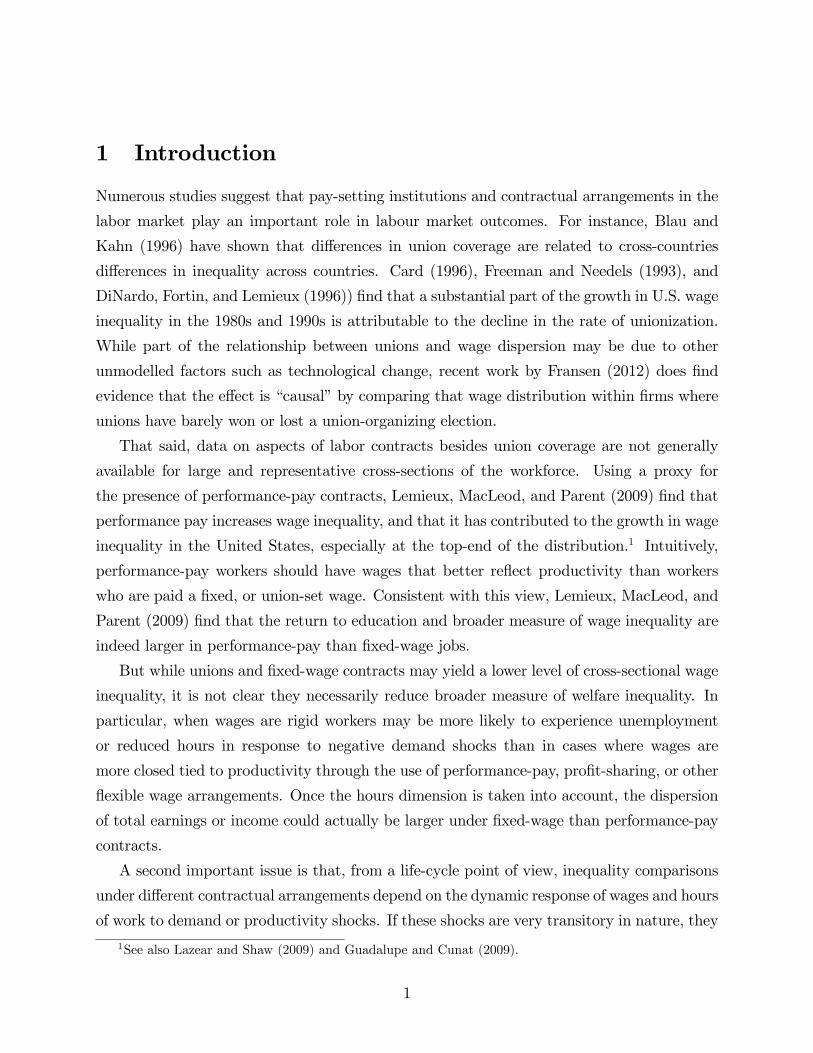
1 Introduction

Numerous studies suggest that pay-setting institutions and contractual arrangements in the

labor market play an important role in labour market outcomes. For instance, Blau and

Kahn (1996) have shown that di¤erences in union coverage are related to cross-countries

di¤erences in inequality across countries. Card (1996), Freeman and Needels (1993), and

DiNardo, Fortin, and Lemieux (1996)) �nd that a substantial part of the growth in U.S. wage

inequality in the 1980s and 1990s is attributable to the decline in the rate of unionization.

While part of the relationship between unions and wage dispersion may be due to other

unmodelled factors such as technological change, recent work by Fransen (2012) does �nd

evidence that the e¤ect is �causal�by comparing that wage distribution within �rms where

unions have barely won or lost a union-organizing election.

That said, data on aspects of labor contracts besides union coverage are not generally

available for large and representative cross-sections of the workforce. Using a proxy for

the presence of performance-pay contracts, Lemieux, MacLeod, and Parent (2009) �nd that

performance pay increases wage inequality, and that it has contributed to the growth in wage

inequality in the United States, especially at the top-end of the distribution.1 Intuitively,

performance-pay workers should have wages that better re�ect productivity than workers

who are paid a �xed, or union-set wage. Consistent with this view, Lemieux, MacLeod, and

Parent (2009) �nd that the return to education and broader measure of wage inequality are

indeed larger in performance-pay than �xed-wage jobs.

But while unions and �xed-wage contracts may yield a lower level of cross-sectional wage

inequality, it is not clear they necessarily reduce broader measure of welfare inequality. In

particular, when wages are rigid workers may be more likely to experience unemployment

or reduced hours in response to negative demand shocks than in cases where wages are

more closed tied to productivity through the use of performance-pay, pro�t-sharing, or other

�exible wage arrangements. Once the hours dimension is taken into account, the dispersion

of total earnings or income could actually be larger under �xed-wage than performance-pay

contracts.

A second important issue is that, from a life-cycle point of view, inequality comparisons

under di¤erent contractual arrangements depend on the dynamic response of wages and hours

of work to demand or productivity shocks. If these shocks are very transitory in nature, they

1See also Lazear and Shaw (2009) and Guadalupe and Cunat (2009).

1

only yield short-term variability in earnings that has little impact on welfare over the whole

life cycle. In such a setting, one has to look at the whole autocovariance structure of earnings

and hours to assess the full impact of contractual arrangements on welfare.

In this paper, we use data from the Panel Study of Income Dynamics (PSID) to look

at how dimensions of contractual arrangements �performance-pay and, to a smaller ex-

tent, unionization�a¤ect the whole autocovariance structure of earnings and hours. A �rst

important �nding is that the cross-sectional variance of annual earnings is smaller under

performance-pay contracts, which is the opposite of what Lemieux, MacLeod, and Parent

(2009) found in the case of hourly wages. We interpret this as evidence that �xed-wage

contracts result in involuntary unemployment, thereby increasing the dispersion in annual

earnings among workers.

We then turn to a full analysis of the autocovariance structure of hourly wages and annual

earnings. Descriptive evidence indicates that while the variance of annual earnings is large

in �xed-wage than performance-pay jobs, this is all due to a higher transitory dispersion in

earnings that lasts for no more than a few years. Estimates based on an error-components

model con�rm this descriptive evidence. We �nd that the variance of the permanent com-

ponent of either hourly wages of annual earnings is larger in performance-pay than �xed-wage

jobs because skills are more rewarded in the former type of jobs. By contrast, the variance

of the transitory component of annual earnings is larger in �xed-wage jobs. This is consist-

ent with transitory demand or productivity shocks generating a large variability in hours

of work in �xed-wage jobs. These results are robust to a variety of speci�cations allowing

for time-varying factor loadings and worker-�rm match components. We also �nd a similar

pattern of results when comparing union and non-union jobs.

The rest of the paper proceeds as follows. In Section 2, we propose a simple model

where contracts are used to protect speci�c investments. Because of asymmetric information,

employers can either o¤er a �xed-wage contract, which potentially generates involuntary

unemployment, or pay a �xed monitoring cost and o¤er a performance-pay contract instead.

We discuss how wages and hours respond to various shocks under these two contractual

arrangements, and derive the implications of the model on the covariance structure of hours

wage wages.

In Section 3 we present the error-component model we use to parametrize the autocov-

ariance structure of hours and wages, and test the predictions of the model under di¤erent

2

contractual arrangements. In Section 4 we discuss how we measure contract form using the

PSID data, and present some descriptive evidence on wages, earnings, and hours of work for

performance-pay and �xed-wage jobs. The main estimation results are presented in Section

5, and we conclude in Section 6.

2 Theory

Before discussing how we expect the distribution of earnings and wages and their autocov-

ariance structure to di¤er under various contractual arrangements, it is important to explain

why we expect these contractual arrangements to arise in the �rst place. In the �rst part of

this section, we present a simple explanation based on the need for contractual arrangements

in the presence of relationship speci�c investment. This simple model also has straightfor-

ward predictions on how wages and hours are expected to respond to demand or productivity

shocks. We then discuss a more general case with heterogenous workers to get a full set of

implications for the whole distribution of earnings and wages, as well as their autocovariance

structure.

2.1 Speci�c investments, asymmetric information, and monitoring

costs

This part of the paper relies heavily on Lemieux, MacLeod, and Parent (2012). We build

a very simple labor contracting model using three ingredients. The �rst is the existence of

relationship speci�c investment that both Becker (1962) and Mincer (1962) emphasized as

central to the wage setting process. The second ingredient is contract law for which the

protection of speci�c investments, or what legal scholars call the �reliance interest� (see

Fuller and Perdue (1936)). In particular, if a worker makes an investment, such as moving

to take up a job or acquiring some job-speci�c skills, an employer cannot after the fact

unilaterally reduce wages. Legal doctrines, such as good faith and fair dealing, explicitly

limit the scope of �rms to reduce wages.2 When employment contracts cannot be enforced,

and �rms can unilaterally lower wages, this leads to what Goldberg (1977) calls �holdup�,

which can result in an ine¢ ciently low level of reliance by both the worker and the �rm.

2In Rigby v Ferodo [1988] ICR 29, [1987] IRLR 516 the U.K. courts ruled that employers could not

unilaterally lower wages.

3

The �nal ingredient is asymmetric information. Hart and Moore (1988) have shown that

when there is symmetric information, and contracts are incomplete, then rational parties

would always renegotiate ine¢ cient agreements, leading to e¢ cient employment ex post,

which in turn leads to ine¢ cient investment ex ante. MacLeod and Malcomson (1993)

apply these ideas to the employment contract and show that the optimal contract entails

�xed wages that are renegotiated in the face of better market alternatives for the worker or the

�rm. Contracts can be designed to achieve e¢ ciency in a wide variety of cases, including the

case of cooperative investment - one party�s investment a¤ecting both parties�payo¤. Such

a model, like implicit contract theory, cannot by itself explain ine¢ cient unemployment.

(Hart (1988) explicitly makes the point that asymmetric information is central to a theory

of unemployment). Following Hall and Lazear (1984), we suppose that there is asymmetric

information, which makes it impossible for �rms to e¢ ciently modify wages ex post. Here,

we combine asymmetric information regarding worker productivity with relationship-speci�c

investments to produce a simple model where wages are set in advance, and employment is

lower than the �rst best.3

When the measurement of worker productivity is possible, ine¢ cient unemployment

linked to �xed wages can be eliminated by introducing bonus pay. Our key identifying

assumption is that monitoring costs vary across �rms.4 This allows us to compare empir-

ically performance-pay and �xed-wage jobs, holding worker quality �xed. In this case, the

model predicts that bonus-pay workers are more likely to be employed than workers on �xed-

wage jobs. Furthermore, demand shocks should have a larger impact on wages and a smaller

impact on employment for bonus-pay workers.

More formally, consider a two-period model that illustrates the consequences of speci�c

investment, enforceable wage contracts and asymmetric information, the details of which are

found in the model appendix. The timing of choices is as follows:

1. In period 1 the worker can accept a wage o¤er w1 from �rm A or B and then make

a speci�c investment k1 - in order to avoid hold-up the �rms agrees not to lower the

wage in period 2. Firm A pays a monitoring cost c to produce a publicly observable

3This is consistent with Card (1986) who �nds that wages are rigid in the short run.4Brown (1992) found that the assumption that there is a common �xed cost of monitoring is inconsistent

with the evidence, while MacLeod and Parent (1999) show that bonus pay is wide spread in the labor market,

with its incidence varying with job characteristics.

4

signal s 2 f0; 1g that is positively correlated with �rm productivity. Firm A agrees to

pay a bonus b if s = 1.

2. If the worker rejects both o¤ers, then she waits until the �rms realize their productiv-

ities and make new wage o¤ers based upon these realized productivities. She can take

up either o¤er at cost k2 > k1.

3. If she accepts the o¤er from say A, then in period 2 �rm B can o¤er a new wage w2

based on its productivity that she can choose to accept at a cost k2.

4. Before production begins, �rms can choose to layo¤ workers. Since �rm productivity

is private information, workers will refuse to renegotiate wages down in the event the

�rm has low productivity. Such behavior is a necessary ingredient of any wage contract

consummated in period 1.

Suppose that ex ante the worker is better matched at A. This model illustrates in the

most simple form the trade-o¤ between early investment into �rm A, against the option

value of delaying investment if it turns out that either �rm B or exit from the labor market

is ex post optimal. Notice that asymmetric information is a key ingredient here. If worker

productivity is information that is private to the �rm, then workers would never agree to

wage cuts because the �rm may simply be misrepresenting its costs. Wages can only respond

to credible signals, such as a wage o¤er from another �rm.5

The model generates a number of empirical implications -discussed in the appendix-

on how contract form matters for wages and employment. Most importantly, we expect

employment to be higher and less responsive to demand shocks in performance-pay jobs

since �xed-wage workers get laid o¤whenever productivity falls below w1. The presence of a

bonus makes the wage rate (inclusive of bonus) more sensitive to demand shocks than under

�xed wages, and hence the worker faces a lower probability of layo¤ under performance pay.

2.2 Heterogenous workers

Now consider what happens when workers are heterogenous, and both �rms and workers

only have imperfect information about workers�productive ability. Lemieux, MacLeod, and

5See Carmichael and MacLeod (2003) for a discussion of the credibility of such behavior when contracts

are not legally enforceable.

5

Parent (2009) have looked at this issue in a simple model where information is imperfect

but symmetric, and where performance pay also provides an incentive for workers to provide

e¤ort. While generalizing this model to the dynamic case with speci�c investments and

asymmetric information about demand shocks is beyond the scope of this paper, we believe

that most of the predictions derived by Lemieux, MacLeod, and Parent (2009) would still

hold here.

In the presence of imperfect information, �xed-wage contracts will be based on the expec-

ted productivity of the worker given the information available at the time the worker is hired.

In principle, the worker and the employer could learn about the productivity of the worker

with the passage of time, as in a standard Jovanovic learning model. In the absence of an

explicit measurement technology, however, learning about workers�productivity is expected

to happen at a much slower rate than in performance-pay jobs. For the sake of simplicity, we

ignore these dynamic considerations here and simply assume that �xed-wage contract pay

a wage equal to the expected value of output at the time the worker is hired. Likewise, the

base wage in a performance-pay contract would also depend on expected productivity, but

the bonus part of the contract would depend on actual productivity that is (imperfectly)

captured by the signal s.

The important implication of this assumption is that wages will be more dispersed in

performance-pay than �xed-wage jobs. For a given information set available at the time the

worker is hired, more productive workers will get a positive productivity signal more often

than less productive workers. As a result, they will be more likely to receive a bonus, which

will increase wage (inclusive of bonus) dispersion among workers with similar characteristics.

Intuitively, wages are more dispersed among performance-pay workers because they are more

closely tied to productivity than in �xed-wage jobs.

2.3 Wage setting equations

Consider the (log) wage of worker i at time t under a performance-pay contract:

wpit = ap + xitb

p + cpuit + dp�i + "

pit; (1)

where xit represents standard observable characteristics such as potential experience, edu-

cation, occupation, �i is the unobservable ability component; uit is a productivity (or other

6

demand-side) shock; "pit is an idiosyncratic error term. Similarly, the wage under a �xed-wage

contracts (i.e. on a �non-performance-pay jobs�) is given by

wnit = an + xitb

n + cnuit + dn�i + "

nit: (2)

When wages are completely �xed in advance, we expect the shock uit to have no e¤ect on

wages at all, and cn to be equal to zero. By contrast, under performance pay at least part

of the shock should be passed on to wages, so that cn > 0. As we discuss in the data section,

however, we only have imperfect measures of whether workers are on performance-pay or

�xed-wage contracts. Therefore, we don�t generally expect to �nd that cn = 0 in the data.

That said, if the way we divide performance-pay and �xed-wage jobs is informative we should

still expect to �nd cp > cn. In light of our discussion of the case of heterogenous workers, we

also expect that the factor loading on both observable characteristics and unobserved ability

to be larger in performance-pay and �xed-wage jobs, i.e. bp > bn and dp > dn.

Now at consider the case of annual earnings for performance-pay

ypit = apy + xitb

py + c

pyuit + d

py�i + �

pit; (3)

and �xed-wage workers:

ynit = any + xitb

ny + c

nyuit + d

ny�i + �

nit: (4)

As we discussed above, a shock uit should have a larger impact on annual hours of work

under �xed-wage contracts since none of the adjustment to, say, a negative shock is absorbed

in terms of lower wages. Depending on how large the hours adjustment is relative to the

wage adjustment, cny may either be larger or smaller than cpy. By contrast, we still expect the

factor loadings on xit and �i to be larger in performance-pay than �xed-wage jobs (bpy > bny

and dpy > dny ). The intuition is that, if anything, paying a higher wage to higher ability

workers should make them work more hours if the labor supply elasticity is positive.

Note that since we are working in logs, annual hours in performance-pay and �xed wage

jobs are given by hpit = ypit � w

pit and h

nit = y

nit � wnit. As a matter of convenience, we prefer

working with wages and earnings, but the exact same results would be obtained working

with wages and hours instead.

7

2.4 Unions

At this stage, we simply view unionization as an additional indicator of the type of contract

involved. While the above model draws a sharp contrast between performance-pay and

�xed-wage contracts, we will see below that there are some di¢ culties in measuring these

two concepts empirically. For simplicity, we expect that unionization gets us even closer

to a �xed-wage setting, since collective bargaining agreements indeed tend to pre-specify

wages over the duration of the contract (2-3 years, often more in recent years). Interestingly,

however, some union contracts allow for a limited amount of pay-for-performance, which

generates more �exibility in response to labor market shocks.

In practice, we divide contracts into up to four categories based on union and performance-

pay status. We expect union contracts without performance pay to exhibit the least wage

�exibility and the largest hours response, and non-union contracts with performance pay to

be the most �exible.

3 Empirical Model for the Autocovariance Structure

of Wages and Earnings

The c and d parameters (factor loadings) in equations (1), (2), (3), and (4) determine

how demand shocks uit and unobserved ability �i map into wages and earnings. Since we

expect demand shocks to be transitory while unobserved ability is a permanent component

of the error term, the factor loadings have important implications for the nature of wage

and earnings inequality. A larger d factor loading increases the permanent component of

inequality, while a larger c factor loading increases transitory inequality.

Starting with Mo¢ tt and Gottschalk (1994), there is a large literature that seeks to

examine whether the large increase in U.S. wage inequality is driven by the transitory or

permanent component of inequality. Knowing which of the two components accounts for the

bulk of the growth inequality has important implications in terms of welfare.

Our focus is slightly di¤erent here since we are not primarily interested in understanding

why inequality has increased over the last few decades. Our main focus is instead in estim-

ating the impact of contract form on the transitory and permanent components of wage and

earnings inequality. That said, our analysis has some indirect implications for this debate

8

since contract form has been changing over time with the decline of unionization and the

growth of performance-pay contracts (Lemieux, MacLeod, and Parent (2009), Bloom and

Van Reenen (2011), and Dube and Freeman (2011)).

We explore these issues formally by estimating parametric models for the autocovariance

structure of wages and earnings. As is common in this literature (e.g. Abowd and Card

(1989)), we �rst �residualize�wages and earnings by running regressions on a rich set of

covariates such as experience, education, etc.6 Note that we are focusing our analysis on the

�residual� or �within-group� component of inequality, as opposed to the more systematic

�between-group�component. Lemieux, MacLeod, and Parent (2009) show that performance-

pay also tends to increase between-group inequality (higher return to education) and, thus,

the permanent component of inequality. We don�t look at this inequality component here

since we are more interested in the impact of idiosyncratic demand/productivity shocks that

a¤ect the within- as opposed to the between-group component of wages and earnings.

Following Lemieux, MacLeod, and Parent (2009), we also consider a possible job-match

component �ij in the wage and earnings equation. In their model, the variance of the job-

match component is expected to be lower in performance-pay than other jobs. The idea is

that when workers are paid for performance, the particular job they have should not matter

as much as their own productive ability. Our main focus here is simply to control for that

variance component to make sure it does not confound the estimates of the variance of

unobserved heterogeneity (V ar(�i)) and demand shocks (V ar(uit)).

Consider the residual wage for performance-pay jobs, ewpijt:ewpijt = cpuit + dp�i + �pij + "pit; (5)

and for non-performance-pay jobs, ewnijt, is:ewnijt = cnuit + dn�i + �nij + "nit; (6)

where the subscript j refers to the job (i.e. the employer-employee or job-match). The

corresponding equations in the case of earnings are:

eypijt = cpyuit + dpy�i + �pij + �pit; (7)

6As we explain in the data section, because of data limitations we only estimate our models for men. The

covariates used to residualize the wage and earnings data are polynomials (cubic) in potential experience and

tenure, years of completed schooling, and dummies for occupation, industry, race, marital status, collective

bargaining, and calendar year.

9

and eynijt = cnyuit + dny�i + �nij + �nit; (8)

We estimate the model under the simplifying assumption that the idiosyncratic error

terms "pit and "nit are uncorrelated over time. These error terms could either re�ect meas-

urement error, or purely transitory shocks. A simple approach for distinguishing the de-

mand/productivity shocks uit from the idiosyncratic errors is to assume some (limited) per-

sistence in uit. For instance, we consider the AR(1) model:

uit = �uit�1 + !it; (9)

where !it is uncorrelated over time.

In some speci�cations, following the existing literature (e.g. Baker and Solon (2003)) we

also allow the factor loadings d and the variance of the idiosyncratic errors to vary over time.

This helps capture changes in returns to (unobserved) skills and related factors that have

been linked to the secular growth in wage and earnings inequality.

Following Parent (2002), we estimate the variance components by �tting regression mod-

els to all the cross-products of residuals for the same individual.7 This procedure is similar to

the equally-weighted minimum distance approach of Abowd and Card (1989), but provides

an easy way of dealing with an unbalanced sample like ours.

To see how the variance components models are identi�ed, consider the expected value of

the di¤erent cross-products of the wage residuals in the case where the factor loadings (the

d�s) do not change over time. For individuals on performance-pay jobs, the expected value

of the squared residuals is

E( ewpijt � ewpijt) = (cp)2 var(uit) + (dp)2 � var(�i) + var(�pij) + var("pijt):The expected value of cross-products for two observations (at time t and time s) on the

same job j is

E( ewpijt � ewpijs) = �t�s (cp)2 var(uit) + (dp)2 � var(�i) + var(�pij);and the expected value of cross-products for two observations on di¤erent jobs j and k is

E( ewpijt � ewpijs) = �t�s (cp)2 var(uit) + (dp)2 � var(�i)7See Parent (1999) for a related analysis with the NLSY comparing piece-rate/commission workers and

those receiving bonuses to salaried and hourly paid workers.

10

In this simple example, we can estimate the four variance components (cp)2 var(uit),

(dp)2var(�i), var(�pij) and var("

pijt) as well as the AR(1) parameter � by �tting the model

using non-linear least squares. The same procedure can then be used to estimate the corres-

ponding parameters for �xed-wage workers, and for the annual earnings models.

If the variance of uit and �i were the same for performance-pay and �xed-wage workers, it

would be straightforward to estimate all the c and d loading factors subject to a normalization

such as cp = dp = 1. With cp = 1 we can identify var(uit) from the wage model for

performance-pay workers. The other loading factors (cn; cpy; cpy) can then be estimated as the

ratio of the squared root of the variances.

The variance of uit and �i being the same for performance-pay and �xed-wage workers is

a strong assumption, however. Unless workers are randomly selected into performance-pay

jobs, we expect the variance of unobserved ability, var(�i), to be di¤erent for the two types

of jobs. We deal with the problem empirically by restricting the estimation to �switchers�

who are observed on both types of jobs. This ensures that var(�i) is the same on the two

types of jobs, and that di¤erence in these variances is due to the loading factors as opposed

to unobserved heterogeneity.

It is harder to deal with potential di¤erences in the variance of shocks, var(uit), in the

two types of jobs since the choice of contract form may also depend on that parameter. In

light of this, di¤erences in the variance of shocks in the two types of jobs has to be interpreted

with caution. That said, under the weaker assumption that wages and earnings for a given

worker are subject to the same shock uit, we can still identify the ratio of factor loadings

cpy=cp and cny=c

n as the square root of the estimated variances. For instance, if most of the

shocks in performance-pay jobs are absorbed in terms of lower (or higher) wages and hours

are relatively una¤ected, we will have cpy=cp � 1. By contrast, if hours are the main margin

of adjustment in �xed-wage jobs, we should �nd that cny=cn >> 1 since shocks will generate

large variance in annual earnings (factor loading cny ), and little variance in hourly wages

(factor loading cn).

4 Data and motivating evidence

Our analysis is conducted using data from the PSID. The main advantage of the PSID is that

it provides a representative sample of the workforce for a relatively long time period. One

11

disadvantage of the PSID is that our constructed measures of performance pay are relatively

crude for reasons discussed below.

4.1 The Panel Study of Income Dynamics (1976-1998)

The PSID sample we use consists of male heads of households aged 18 to 65 with average

hourly earnings between $1.50 and $100.00 (in 1979 dollars) for the years 1976-1998, where

the hourly wage rate is obtained by dividing total labor earnings from all jobs by total

hours of work, both reported retrospectively for the previous calendar year.8,9 Given our

focus on performance pay, this wage measure based on total yearly earnings, inclusive of

performance pay, is preferable to �point-in-time� wage measures that would likely miss

infrequent payments (e.g. bonuses) of performance pay.

Individuals who are self-employed are excluded from the analysis since our measure of

performance pay based on receiving bonuses, commissions, or piece-rates is de�ned for em-

ployed workers only.10 We also exclude workers from the public sector. This leaves us with a

total sample of 27,899 observations for 3,131 workers. Note that we only keep observations

where individuals have worked a positive number of hours during the year, and record pos-

itive earnings. While this sample exhibit a large amount of variation in annual hours due to

spells of unemployment, etc., we exclude the cases where people don�t work at all during the

year since wages are not observed in that case. In some speci�cations we also focus on a more

8In the PSID, data on hours worked during year t, as well as on total labor earnings, bo-

nuses/commissions/overtime income, and overtime hours, are asked in interview year t+1. Thus we actually

use data covering interview years 1976-1999. Annual earnings were top coded at $99,999 until 1982 (and not

top coded since then), but only a handful of individuals were at the top code. We trim very high values of

wages (above $100.00 in 1979 dollars) but do not otherwise adjust for top coding.9Our focus on male heads of households stems from the fact that only heads are asked about their

income derived from bonuses, commissions, or overtime. In the PSID, males are designated as the head in

all husband-wife pairs. The same is true if the female has a boyfriend with whom she has been living for

at least a year, even if the female is the person with the most �nancial responsibility in the family unit.

Consequently, the sample of female heads is relatively small. Using the same sample selection criteria as

the ones we use for males would leave us with 1,367 females for a total of 8,185 observations. Perhaps more

importantly, issues of representativeness would arise as those female heads are disproportionately nonwhite

(24.4 percent) and are much less likely to be married (9.2 percent).10Self-employed workers can be viewed as being, by de�nition, paid for performance regardless of the

mode of payment (earnings, dividends, etc.) they use to remunerate themselves.

12

�stable�subsample of workers who are employed at the time of the interview. The sample

size drops to 26,146 observations, meaning that in 1753 cases we have workers unemployed

at the interview who, nonetheless, still end up working a positive number of hours during

the year. All of the estimates reported in the paper are weighted using the PSID sample

weights.

Identifying Performance Pay We construct a performance-pay indicator variable by

looking at whether part of a worker�s total compensation includes a variable pay component

(bonus, commission, or piece-rate). For interview years 1976-1992, we are able to determine

whether a worker received a bonus or a commission over the previous calendar year through

the use of multiple questions. First, workers are asked the amount of money they received

from working overtime, from commissions, or from bonuses paid by the employer.11 Second,

we sometimes know only whether or not workers worked overtime, and if they are working

overtime in a given year, not the amount of pay they received for overtime. Thus, we

classify workers as not having had a variable pay component if they worked overtime. Third,

workers not paid exclusively by the hour, or not exclusively by a salary, are asked how they

are paid: they can report being paid commissions, piece-rates, etc., as well as a combination

of salaried/hourly pay along with piece-rates or commissions.12 Through this combination

of questions, we are thus able to identify all non-overtime workers who received performance

pay in bonus, commission, or piece-rate form.

Starting with interview year 1993, there are separate questions about the amounts earned

in bonuses, commissions, tips, and overtime for the previous calendar year. Thus, there is

no need to back out an estimate of bonuses from an aggregate amount since the question is

asked directly. For the sake of comparability with the pre-1993 years, we nevertheless classify

11Note that the question refers speci�cally to any amounts earned from bonuses, overtime, or commissions

in addition to wages and salaries earned.12In many survey years workers are not asked if their compensation package involves a mixture of

salary/hourly pay and a variable component. All they are asked is how they are paid if not by the hour or

with a salary. Although there is no way to directly verify it, this likely results in understating the incidence

of any form of variable pay because workers are not allowed to answer that they are paid, say, a salary, and

then report a commission: they have to choose. Our assertion that this response likely understates the extent

of variable pay is motivated in part by the fact that workers in the NLSY are not restricted in describing

the way they are paid. We �nd that workers in the NLSY are more likely to report having part of their

compensation package contain a performance-pay component.

13

as receiving no performance pay all workers who report any overtime work. In this way we

are able to determine whether a worker�s total compensation included a performance-pay

component for each year of the survey. One obvious drawback is that it is likely that the

performance-pay component we construct will be noisy for hourly workers, though not for

salaried workers who are not eligible for overtime payments. However, due to our treatment

of overtime workers, we conservatively lean on the side of misclassifying workers as receiving

no performance pay even when they do.13

De�ning Performance-pay Jobs We de�ne performance-pay jobs as employment rela-

tionships in which part of the worker�s total compensation includes a variable pay component

(bonus, a commission, piece-rate) at least once during the course of the relationship.14 Since

we use actual payments of bonuses, commissions or piece rates to identify performance-

pay jobs, we are likely to misclassify performance-pay jobs as non-performance-pay jobs if

some employment relationships are either terminated before performance pay is received,

or partly unobserved for being out of our sample range. This source of measurement error

is problematic because of an �end-point�problem in the PSID data. Given our de�nition

of performance-pay jobs, we may mechanically understate the fraction of workers in such

jobs at the beginning of our sample period because most employment relationships observed

in 1976 started before 1976, and we do not observe whether or not performance pay was

received prior to 1976. Similarly, jobs that started toward the end of the sample period

may be performance-pay jobs but are classi�ed otherwise because they have not lasted long

enough for performance pay to be observed.

The problem is that, conditional on job duration, we tend to observe a given job match

fewer times at the two ends of our sample period than in the middle of the sample. Consider,

for example, the case of a job that lasts for �ve years. For jobs that last from 1985 to 1989,

13In an earlier version of the paper, we re-did the analysis for 1992 to 1998 using the �ner measure of

performance pay that allows us to identify the performance-pay status of overtime workers. Doing so had

little impact on the results. It only increased the fraction of workers on performance-pay jobs (for 1992-98)

by one percentage point, and regression coe¢ cients were essentially unchanged.14We use �jobs�, �employment relationship�, and �job match�interchangeably. Although the PSID does

have information on tenure in the position in most of the survey years spanning the sample period, we do not

use it. As is well known, simply determining employer tenure in the PSID can be problematic (see Brown

and Light (1992)). As a result, what we call a �job match�could be called an �employer match� instead.

We generally use the word �job�for the sake of simplicity.

14

all �ve observations on this job match are captured in our PSID sample. For jobs that last

from 1973 to 1977, however, only two of the �ve years of the job match are observed, which

mechanically reduces the probability of classifying the job as one with performance pay.

Because of this end-point problem, we get an unbalanced distribution of the number of

times job matches are observed at di¤erent points of the sample period. One simple solution

to the problem is to �rebalance�the sample using regression or other methods. In practice,

we adjust measures of the incidence of performance pay over time by estimating a linear

probability model in which dummies for calendar years and for the number of times the

job-match is observed are included as regressors (estimating a logit gave almost identical

results). We then compute an adjusted measure of the incidence of performance pay by

holding the distribution of the number of times the job-match is observed to its average

value for the years 1982 to 1990, which are relatively una¤ected by the end-point problem.

The end-point problem could also a¤ect the estimates of the e¤ect of performance pay

on both wage, hours, and earnings because the sample of non-performance-pay jobs is be-

ing contaminated by observations from performance-pay jobs for which performance-based

payments are never observed. Lemieux, MacLeod, and Parent (2009) have investigated this

issue in detail and concluded that, if anything, this measurement problem biases downward

the estimated e¤ect of performance pay. For the sake of clarity and simplicity, the wage

samples we work with in the next sections are unadjusted for these measurement issues.

4.2 Descriptive Statistics from the PSID

Table 1 compares the mean characteristics of workers on performance-pay and non-performance-

pay jobs, respectively. First, notice that 36 percent of the 27,899 observations are in

performance-pay jobs. Workers on performance-pay jobs tend to earn more and have higher

levels of education than workers on non-performance-pay jobs. Note that the hourly wage

rate includes both regular wage and salary earnings and performance pay in the case of

workers on performance-pay jobs. Annual hours worked and employer tenure also tend to

be higher for workers on performance-pay than non-performance-pay jobs.

The unionization rate (percent covered by a collective bargaining agreement) is much

lower among performance-pay workers. This suggests that, as expected, the pay structure

in union �rms corresponds more closely to the �xed-wage contracts discussed in Section

2. Another important di¤erence is that there is a much higher fraction of workers paid

15

by the hour in non-performance-pay than performance-pay jobs. Conversely, workers on

performance-pay jobs are more likely to be salaried workers than those on non-performance-

pay jobs.

An important point illustrated at the bottom of the table is that, of the 3131 workers, 1318

are observed on a performance-pay job, and 2715 are observed on a non-performance-pay

job. So 902 workers (1318+2715-3131) are �switchers�observed on both types of jobs. As

discussed above, we present estimates of the variance components models for this subsample

to control for potential di¤erences in the unobserved ability of workers on the two types of

jobs.

Figure 1 shows the incidence of performance pay over the 1976-98 sample period. Note

that we correct for the end-point problem using the procedure described above. Figure 1

shows that the overall incidence of performance-pay jobs has increased from about 35 percent

in the late 1970s to around 45 percent in the 1990s. The �gure also shows the simpler measure

based on the fraction of workers actually reporting performance pay in a given year. This

alternative measure clearly understates the incidence of performance-pay jobs since workers

on performance-pay jobs will not necessarily receive a performance payment (like a bonus)

in each year on the job. One advantage of this simple measure, however, is that it is not

a¤ected by the end-point problem and provides additional evidence of the robustness of the

underlying trends in performance pay. Indeed, even this crude measure of performance pay

clearly increases over time, especially in the 1980s.

Figure 1 also shows the fraction of workers covered by a collective bargaining agreement.

Interestingly, the decline in unionization and the growth in performance pay are both con-

centrated in the same period (the 1980s). Figure 2 presents kernel density estimates of the

distribution of annual hours for performance-pay and non-performance-pay jobs. The �gure

shows that annual hours have a higher mean and median, and are less evenly distributed

among performance-pay than non-performance-pay jobs.

Note that performance pay represents a relatively modest share of total earnings (Fig-

ure 3). However, this does not mean that performance pay has a limited impact on total

compensation since we expect the straight wage component to be more sensitive to work-

ers�characteristics on performance-pay than non-performance-pay jobs. In order to pay for

performance, the employer must evaluate the worker, which then a¤ects the straight wage

through promotions and job assignment. Hence, even though performance pay is a relatively

16

small fraction of compensation for most workers, the fact that it exists is a signal of more

careful monitoring.

4.3 Local unemployment rate as a measure of shocks

Before turning to the main empirical analysis based on the estimation of variance compon-

ents models, we provide some motivating evidence using an observable measure of shocks.

Following Lemieux, MacLeod, and Parent (2012), we use the local unemployment rate as

a measure of shocks. A simple implication of the model in Section 2 is that the local un-

employment rate should have a larger impact on wages in performance-pay than �xed-wage

jobs, while the opposite should happen in the case of hours. It is not clear, however, how

the impact on the two types of jobs should compare in the case of earnings. As discussed in

Section 2, this depends on the elasticity of labor supply.

The results are reported in Tables 2 and 3. All models include a large set of covariates

that are not reported in the table: polynomials (cubic) in potential experience and tenure,

years of completed schooling, and dummies for occupation, industry, race, marital status,

collective bargaining, and calendar year. Standard errors are clustered at the county-year

level.

In all regression models we show three sets of models for two di¤erent sample of workers.

We start with simple OLS estimates, then move to models with worker-speci�c �xed e¤ects

that capture unobserved ability �i, and then report models with a full set of job match e¤ects.

Estimates with job-match e¤ects are particularly credible as they solely rely on di¤erential

variation in the local unemployment rate, after controlling for year e¤ects and job-match

e¤ects to identify the di¤erential responsiveness to unemployment shocks in the di¤erent

types of jobs.

The two sample of workers used are based on whether or not the worker is unemployed

at the time of the interview. In our PSID sample, we only keep workers with at least some

positive earnings and hours of work in the previous calendar year. These workers may or

may not be working at the time of the interview. We �rst report results for the more �stable�

sample of workers employed at the time of the interview in Table 2 (columns 1-3), and then

for the broader sample that also includes workers unemployed at the time of the interview

(columns 4-6).

Panel A of Table 2 shows that, as expected, the unemployment rate has a negative

17

and signi�cant e¤ect of wages in performance-pay jobs, but no signi�cant e¤ect on non-

performance-pay jobs. The estimated coe¢ cient for performance-pay jobs varies across spe-

ci�cation but is generally close to -0.01, suggesting that a one percentage point increase in

the unemployment rate is associated with a one percent decline in the hourly wage.

Panel B of Table 2 shows that precisely the opposite happens in the case of hours of work.

The unemployment rate has a negative and signi�cant impact on hours of work for workers

not paid for performance, but an insigni�cant impact for performance-pay workers. The

latter e¤ect is consistent with a fairly inelastic labor supply elasticity for performance-pay

workers. By contrast, since wages fail to adjust for non-performance-pay jobs, employers

have little choice but to cut back on hours and employment in the presence of adverse

productivity shocks.

The results for hours are in levels. They are not directly comparable to those for wages

(in logs). Since average yearly hours is about 2000, the -10 estimate reported in Panel B

corresponds to a 0.5 percent decline in hours. This is fairly similar in terms of magnitude

to the estimated e¤ect on the wages of performance-pay workers (Panel A of Table 2). It

suggests that the total e¤ect of the unemployment rate on earnings (wages time hours)

should be roughly comparable for performance-pay and non-performance-pay jobs. The

only di¤erence is that the adjustment happens along the wage margin for performance-pay

workers, but along the hours margins for non-performance workers.

This conjecture is con�rmed in Panel C of Table 2, which shows the estimated e¤ect of

the local unemployment rate on the log of annual earnings. In our preferred speci�cation

with job-match �xed e¤ects, the e¤ect of the unemployment rate on annual earnings is equal

to about -.008 for both performance-pay and non-performance pay jobs. This means that a

one percentage point increase in the local unemployment rate reduces earnings by close to

one percent in both sectors. The di¤erence is that hourly wages account for essentially all

the earnings adjustment in performance-pay jobs, while hours account for the bulk of the

adjustment in non-performance-pay jobs.

Table 3 presents similar estimates except that we now divide jobs both in terms of

performance-pay and union status. As discussed in Section 2, we expect wages to be most

responsive to shocks in performance-pay jobs that are not unionized, and least responsive to

shocks in unionized non-performance-pay jobs. We also expect the exact opposite to happen

for hours of work. The two other types of contractual arrangements (union/performance-pay

18

and non-union/non-performance pay) should fall somewhere in between these two extreme

cases.

Looking once again at our preferred speci�cation (column 3), we see that the results are

consistent with these expectations. Panel A of Table 3 shows that the unemployment rate

has the largest impact on non-union performance-pay jobs (-0.0076) and the smallest (and

not statistically signi�cant) impact on union non-performance-pay workers (-0.0001). By

contrast, exactly the opposite happens in the case of hours of work (Panel B). As a result,

the overall impact on annual earnings is more or less similar for all four types of contractual

arrangements (Panel C).

One potential concern with these results is that some of the di¤erential responsiveness

to shocks under di¤erential contractual arrangements is due to composition e¤ects. For

example, performance-pay workers tend to be more concentrated in occupations such as

managers and professionals (see Lemieux, MacLeod, and Parent (2009)) that may be less

sensitive to the business cycle than blue collar occupations. One simple way of checking for

this is to rebalance the performance-pay and non-performance pay samples so that they have

the same distribution of observed characteristics. We did so using a reweighting procedure

and this did not substantially changed the results.

5 Main Results

Before turning to the estimation of the variance components model, we show the raw autoco-

variance matrices for wages and earnings in performance-pay and non-performance-pay jobs

in Appendix Table 1 (employed workers at the time of the interview) and 3 (all workers).

A number of interesting patterns can be observed in the raw data. First, cross-sectional

inequality as measured by the variances (zero order covariances on the diagonal) tends to

increase over time, re�ecting the well-known secular growth in inequality. Second, while the

variance of wages is generally larger in performance-pay than non-performance-pay jobs, the

variance increases much more in non-performance-pay jobs when we move to the broader

measure of inequality based on annual earnings. Third, the autocovariances decline slower

when we move o¤ the diagonal for performance-pay than non-performance-pay jobs. This

is particularly striking in the case of earnings and suggests that the larger variance in non-

performance-pay jobs is due to transitory variability in hours.

19

These patterns are easier to see in Figures 4-5 that plot the evolution of the di¤erent

variances over time, and in Appendix Table 2 (and 4) that shows the average values of the

autocovariances. Comparing columns 1 and 2 of Appendix Table 2, it is clear that going

from wages to annual earnings has little impact on the autocovariances in performance-pay

jobs. By contrast, there is a large di¤erence between the autocovariances of wages and

earnings in non-performance-pay jobs (columns 3 and 4). This is consistent with our �nding

in Tables 2-3 that there is much more variation in hours in response to shocks in non-

performance-pay jobs. The di¤erence also diminishes quickly as we increase the order of the

autocovariances, suggesting that most of the variation in hours is transitory. As a result, the

autocovariance in earnings in performance-pay jobs is larger than in non-performance-pay

jobs for all autocovariances except the zero order autocovariance (the variance).

The estimates of the variance components models are reported in Tables 4-8 for various

samples and speci�cations. At this stage we only report estimates from simple models where

shocks uit are assumed to be purely transitory (� = 0). In that context, we cannot separately

estimate the variance of the uit and "it terms (or �it for earnings), and just report the sum

of the two variances in the tables. This corresponds to a conventional variance components

model with a pure transitory and a pure permanent variance component, though we also

include a job-match component in some speci�cations. Preliminary estimates indicate that

estimates of � for the various speci�cations are tightly clustered around 0.8. While allowing

for � 6= 0 greatly improves the �t of the model, it does not change the qualitative conclusionspresented below on the e¤ect of shocks on wages and earnings under the di¤erent types of

contracts.

In all the tables, we �rst report estimates from a simple model where the factor loadings

dpt and dnt are assumed to be �xed over time, and the job-match component is set to zero. We

then add the job-match component in a second speci�cation, and free up the factor loadings

(return to unobserved ability) and the variance of "pijt and "nijt to re�ect the well-known

growth in inequality over time.

In all �ve tables, we �rst report (Panel A) results estimated over the whole sample. As we

discussed earlier, one potential pitfall of using the whole sample is that some individuals are

only observed on performance-pay jobs, while others are only observed on non-performance-

pay jobs. To control for these composition e¤ects, we report in Panel B the results for the

subsample of �switchers�who are observed on both performance-pay and non-performance-

20

pay jobs.

Table 4 shows the results of the wage decomposition for the subsample of more �stable�

workers in employed at the time of the survey (this table is the same as Table 5 in Lemieux,

MacLeod, and Parent (2009)). Consistent with the pattern observed in the empirical auto-

covariances (Appendix Tables 1 and 2), the results con�rm that the permanent component

of wages (variance of �i) is substantially larger in performance-pay than non-performance-

pay jobs. The rest of the tables (Table 5-8) report the results for the broader measure of

inequality based on annual earnings.

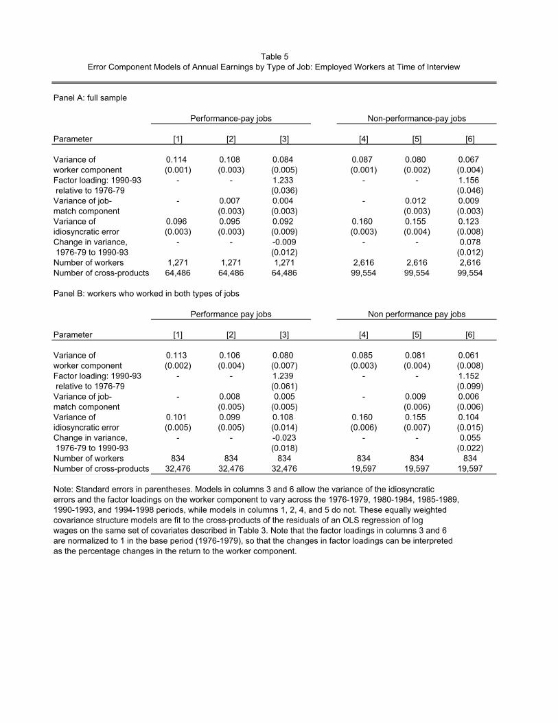
For performance-pay jobs, the variance decomposition of earnings reported in Table 5 is

fairly similar to the decomposition for wages in Table 4. The only noticeable di¤erence is that

the transitory variance (variance of uit and "pijt) is slightly larger than in the wage models.

By contrast, the transitory variance is almost twice as large for earnings than wages in non-

performance-pay jobs, while the permanent variance is only slightly larger. This is consistent

with the pattern of results documented in the raw data reported in Appendix Tables 1 and

2. The transitory variance becomes even larger when workers unemployed at the time of

the interview are also included in the sample in Table 6. Even in that case, however, the

variance linked to the permanent wage component �i remains larger in performance-pay than

non-performance-pay jobs.

Finally, we report in Table 7 and 8 separate results for the four types of contractual

arrangements based on union and performance-pay status. For the sake of simplicity, we focus

our discussion on the simplest models reports in columns 1 and 4. Consistent with the large

literature on unions and wage inequality, both the transitory and permanent components

of inequality tend to be lower in union than non-union jobs (see, e.g., Lemieux (1998)).

Other than this, the results are fairly consistent with those reported in Table 5 and 6. The

permanent component is larger in performance-pay jobs, while the transitory component is

larger in non-performance-pay jobs. This con�rms that the results in Tables 5 and 6 truly

re�ect the role of performance-pay jobs, and not the fact that performance-pay jobs are less

likely to be unionized, and vice versa.

5.1 Implications for welfare inequality

Looking at earnings instead of just hourly wages �rst suggests that inequality is actually smal-

ler in performance-pay than non-performance-pay jobs, contrary to what Lemieux, MacLeod,

21

and Parent (2009) found for hourly wages only. This result only holds, however, for purely

cross-sectional measures of inequality. Since the variation in hours is mostly transitory,

from a welfare point of view inequality likely remains larger in performance-pay than non-

performance-pay jobs. The fact that hours of work are quite volatile and respond more to

shocks in non-performance-pay jobs has a substantial impact on earnings in the short run,

but little impact on long-run measures of both the level and the inequality of earnings.

6 Conclusion

In this paper, we use data from the Panel Study of Income Dynamics to study how the

aucovariance structure of wages and earnings di¤er under di¤erent contractual arrangements.

We divide jobs on the basis of whether they pay for performance, and whether they are

covered by collective bargaining agreements. Using the county unemployment rate as a

proxy for local labor market shocks, we �nd that wages and hours of work respond very

di¤erently to shocks depending on contractual arrangements. Wages are most �exible under

non-union performance-pay contracts, and least �exible under non-performance-pay union

contracts. Precisely the opposite happens in the case of hours of work that are the least

sensitive to shocks under non-union performance-pay contracts, and the most sensitive under

union non-performance-pay contracts.

We then perform a full-�edge variance components analysis. Looking at earnings instead

of just hourly wages suggests that inequality is actually smaller in performance-pay than non-

performance-pay jobs. This result only holds, however, for purely cross-sectional measures

of inequality. Since the variation in hours is mostly transitory, from a welfare point of view

inequality likely remains larger in performance-pay than non-performance-pay jobs. The fact

that hours of work are quite volatile and respond more to shocks in non-performance-pay

jobs has a substantial impact on earnings in the short run, but little impact on long-run

measures of both the level and the inequality of earnings.

References

Abowd, J. M. and D. Card (1989, March). On the covariance structure of earnings and

hours changes. Econometrica 57 (2), 447�480.

22

Baker, M. and G. Solon (2003, April). Earnings dynamics and inequality among canadian

men, 1976-1992: Evidence from longitudinal income tax records. Journal of Labor

Economics 21 (2), 267�88.

Becker, G. (1962, October). Investment in human capital: A theoretical analysis. Journal

of Political Economy 70, 9�49.

Blau, F. D. and L. M. Kahn (1996, August). International di¤erences in male wage inequal-

ity: Institutions versus market forces. Journal of Political Economy 104 (4), 791�836.

Bloom, N. and J. Van Reenen (2011). Human resource management and productivity.

In O. Ashenfelter and D. Card (Eds.), Handbook of Labor Economics, Vol. 4B, pp.

1697�1769. Amsterdam: Elsevier North Holland.

Brown, C. (1992). Wage levels and method of pay. Rand Journal of Economics 23 (3),

366�375.

Brown, J. N. and A. Light (1992). Interpreting panel data on job tenure. Journal of Labor

Economics 10 (2), 219�257.

Card, D. (1986, December). E¢ cient contracts with costly adjustment: Short-run employ-

ment determination for airline mechanics. American Economic Review 76 (5), 1045�

1071.

Card, D. (1996). The e¤ect of unions on the structure of wages: A longitudinal analysis.

Econometrica 64, 957�979.

Carmichael, L. and W. B. MacLeod (2003). Caring about sunk costs: A behavioral solu-

tion to holdup problems with small stakes. Journal of Law, Economics, and Organiz-

ation 19 (1), 106�18.

DiNardo, J., N. Fortin, and T. Lemieux (1996, September). Labor market institutions and

the distribution of wages, 1973-1992: A semiparametric approach. Econometrica 64 (5),

1001�1044.

Dube, A. and R. B. Freeman (2011). Complementarity of shared compensation and

decision-making systems: Evidence from the american labor market. In D. L. Kruse,

R. B. Freeman, and J. R. Blasi (Eds.), Shared Capitalism at Work: Employee Owner-

ship, Pro�t and Gain Sharing, and Broad-based Stock Options, pp. 176�99. Chicago:

University of Chicago Press.

23

Fransen, B. (2012, January). Why unions still matter: The e¤ects of unionization on the

distribution of employee earnings. Working paper, Massachusetts Institute of Techno-

logy.

Freeman, R. B. and K. Needels (1993). Skill di¤erentials in canada in an era of rising

labor market inequality. In D. Card and R. B. Freeman (Eds.), Small Di¤erences that

Matter: Labor Markets and Income Maintenance in Canada and the United States.

Chicago, IL: University of Chicago Press.

Fuller, L. L. and W. Perdue (1936, nov). The reliance interest in contract damages: 1.

The Yale Law Journal 46 (1), 52�96.

Goldberg, V. P. (1977). Competitive bidding and the production of precontract informa-

tion. Bell Journal of Economics 8 (1), 250�61.

Guadalupe, M. and V. Cunat (2009, July). Globalization and the provision of incentives

inside the �rm. Journal of Labor Economics 27 (2), 179�212.

Hall, R. E. and E. P. Lazear (1984, April). The excess sensitivity of layo¤s and quits to

demand. Journal of Labor Economics 2 (2), 233�257.

Hart, O. D. (1988, January). Optimal labour contracts under asymmetric information:

An introduction. Review of Economic Studies 50 (1), 3�35.

Hart, O. D. and J. Moore (1988, July). Incomplete contracts and renegotiation,. Econo-

metrica, 56 (4), 755�785.

Lazear, E. P. and K. L. Shaw (2009). Wage structure, raises and mobility: An introduction

to international comparisons of the structure of wages within and across �rms. In E. P.

Lazear and K. L. Shaw (Eds.), The Structure of Wages: An International Comparison,

pp. 1�57. Chicago, IL: University of Chicago Press.

Lemieux, T. (1998). Estimating the e¤ects of unions on wage inequality in a panel data

model with comparative advantage and nonrandom selection. Journal of Labor Eco-

nomics 16 (2), 261�291.

Lemieux, T., W. B. MacLeod, and D. Parent (2009, February). Performance pay and wage

inequality. Quarterly Journal of Economics 124 (1), 1�49.

Lemieux, T., W. B. MacLeod, and D. Parent (2012, May). Contract form, wage �exibility,

and employment. American Economic Review 102 (3), 526�31.

24

MacLeod, W. and D. Parent (1999). Job characteristics and the form of compensation. In

S. W. Polachek (Ed.), Research in Labor Economics, Volume 18, pp. 177�242. Stam-

ford, Connecticut: JAI Press INC.

MacLeod, W. B. and J. M. Malcomson (1993, September). Investments, holdup, and the

form of market contracts. American Economic Review 83 (4), 811�837.

Mincer, J. (1962). On-the-job training: Cost, returns and some implications. Journal of

Political Economy 70 (5), 50�79.

Mo¢ tt, R. and P. Gottschalk (1994). The growth of earnings instability in the u.s. labor

market. Brookings Papers on Economic Activity 25 (2), 217�272.

Parent, D. (1999, October). Methods of pay and earnings: A longitudinal analysis. Indus-

trial and Labor Relations Review 53 (1).

Parent, D. (2002, July). Matching, human capital, and the covariance structure of earnings.

Labour Economics 9 (3), 375�404.

25

.1.2

.3.4

.5Fr

actio

n of

Sam

ple

76 78 80 82 84 86 88 90 92 94 96 98Year

Performance Pay Received in Current Year Performance Pay Jobs

Covered by Collective Bargaining Agreement

PSID 19761998Figure 1. Performance Pay Job Incidence

29

0.0

005

.001

.001

5

0 1000 2000 3000 4000Annual Hours Worked

Other Jobs

Performance Pay Jobs

PSID 19761998Figure 2. Distribution of Hours Worked

30

0.0

5.1

.15

Frac

tion

0 .05 .1 .15 .2 .25 .3 .35 .4 .45 .5 .55 .6 .65 .7 .75 .8 .85 .9 .95 1share

Vertical Line Indicates Median Share (4.4%)PSID 19761998

Figure 3. Share of Performance Pay in Total Earnings

31

.5.5

5.6

.65

.7.7

5.8

.85

.9S

td D

evia

tion L

og E

arn

ings

76 78 80 82 84 86 88 90 92 94 96 98Year

All Jobs Performance Pay Jobs

Other Jobs

3−year Moving Average

Panel A: Sample Includes Only Employed WorkersFigure 4. Total Log Earnings Inequality

.5.5

5.6

.65

.7.7

5.8

.85

.9S

td D

evia

tion L

og E

arn

ings

76 78 80 82 84 86 88 90 92 94 96 98Year


Other Jobs


Panel B: Sample Includes Employed and Unemployed Workers

32

500

550

600

650

700

Std

Devia

tion in H

ours

Work

ed

76 78 80 82 84 86 88 90 92 94 96 98Year


Other Jobs


Panel A: Sample Includes Only Employed WorkersFigure 5. Inequality in Annual Hours Worked

500

550

600

650

700

Std

Devia

tion in H

ours

Work

ed

76 78 80 82 84 86 88 90 92 94 96 98Year


Other Jobs


Panel B: Sample Includes Employed and Unemployed Workers

33

Non Performance Performance PayPay Jobs Jobs

Average Hourly Earnings ($79) 8.24 10.81

Education 12.49 13.37

Potential Experience 19.57 19.54

Employer Tenure 7.22 9.20

Married 0.71 0.77

Unionized 0.27 0.15

Non White 0.14 0.09

Paid by the Hour 0.63 0.31

Paid a Salary 0.30 0.50

Fraction Unemployed at Interview 0.073 0.018

Annual Hours Worked 2061.6 2272.1

# workers (Tot:3131) 2715 1318

# Job Matches (Tot: 8689) 6819 1870

# Observations (Tot: 27899) 17934 9965

Notes: The sample consists of male household heads aged 18-65 working in private sector, wage and salary jobs. All figures in the table represent sample means.Education, potential experience, and employer tenure are measured in years.Potential experience is defined as age minus education minus 6. Performance-payjobs are employment relationships in which part of the worker's total compensationincludes a variable pay component (bonus, commission, piece rate). Any worker who reports overtime pay is considered to be in a non-performance-pay job. Workersare considered unionized if they are covered by a collective bargaining agreement.Temporarily laid off workers are included among the unemployed. Forunemployed workers at the time of the interview, the type of job they haverefers to the last job they had.

Table 1. Summary Statistics: Panel Study of Income Dynamics 1976-1998

Panel A: Log Hourly Earnings

Sample:

[1] [2] [3] [4] [5] [6]Fixed-Effects Fixed-Effects Fixed-Effects Fixed-Effects

Variable OLS Within Worker Within Employer OLS Within Worker Within Employer

Unemployment Rate in County -0.0030 -0.0066 -0.0021 -0.0027 -0.0075 -0.0023X Non Performance Pay Job (0.0016) (0.0016) (0.0016) (0.0016) (0.0016) (0.0016)

Unemp. Rate in County X -0.0113 -0.0148 -0.0072 -0.0097 -0.0153 -0.0082Performance Pay Job (0.0022) (0.0020) (0.0021) (0.0022) (0.0020) (0.0021)

P-Value of Test of Equality 0.0009 0.0010 0.0490 0.0050 0.0022 0.0246

Unemployed at Interview - - - -0.1110 -0.0400 -0.0447(0.0194) (0.0165) (0.0255)


Unemp. Rate in County X -0.11 1.68 1.22 0.47 1.43 1.41Performance Pay Job (2.30) (2.77) (3.15) (2.27) (2.79) (2.58)



Number of Observations 26146 26146 26146 27899 27899 27899

Table 2. The Effect of Local Labor Market Conditions: PSID, 1976-1998

Employed Individuals All Employed and Unemployed Individuals

Panel B: Annual Hours Worked

Panel C: Log Annual Earnings

Sample:




Unemp. Rate in County X -0.0116 -0.0125 -0.0078 -0.0096 -0.0163 -0.0085Performance Pay Job (0.0023) (0.0018) (0.0017) (0.0023) (0.0021) (0.0021)




Notes. Estimates come from unrestricted regressions in which all covariates are interacted with the performancepay job dummy. Other covariates include polynomials (cubic) in potential experience and tenure, years of completed schooling, and dummies for occupation, industry, race, marital status, collective bargaining, calendar year, and having part of current year's earnings based on performance pay. Standard errors are clustered at the county X year level.

Table 2. The Effect of Local Labor Market Conditions: PSID, 1976-1998 (continuation)


Panel A: Log Hourly Earnings

Sample:



U. Rate X Unionized Workers 0.0162 0.0052 -0.0001 0.0175 0.0047 -0.0001X Non Performance Pay Job (0.0017) (0.0018) (0.0019) (0.0017) (0.0019) (0.0019)

U. Rate X Non-Unionized Workers -0.0124 -0.0122 -0.0036 -0.0117 -0.0128 -0.0036X Non Performance Pay Job (0.0018) (0.0017) (0.0017) (0.0018) (0.0017) (0.0017)

U. Rate X Unionized Workers 0.0095 -0.0101 -0.0040 0.0100 -0.0115 -0.0060X Performance Pay Job (0.0033) (0.0033) (0.0033) (0.0031) (0.0035) (0.0035)

U. Rate X Non-Unionized Workers -0.0145 -0.0154 -0.0076 -0.0138 -0.0160 -0.0084X Performance Pay Job (0.0026) (0.0022) (0.0024) (0.0025) (0.0022) (0.0023)

Panel B: Annual Hours Worked

U. Rate X Unionized Workers -13.32 -14.63 -13.90 -14.71 -15.48 -13.31X Non Performance Pay Job (2.13) (2.77) (6.96) (2.12) (2.73) (3.05)


U. Rate X Unionized Workers 3.19 -2.64 2.77 5.65 0.19 1.64X Performance Pay Job (5.47) (6.79) (6.96) (4.97) (6.11) (6.31)

U. Rate X Non-Unionized Workers -0.14 1.96 1.27 0.05 1.97 0.78X Performance Pay Job (2.51) (2.91) (3.26) (2.54) (2.98) (3.28)


Table 3. The Effect of Local Labor Market Conditions: PSID, 1976-1998; All Sectors


Panel C: Log Annual Earnings

Sample:



U. Rate X Unionized Workers 0.0094 -0.0021 -0.0070 0.0104 -0.0016 -0.0055X Non Performance Pay Job (0.0038) (0.0020) (0.0019) (0.0020) (0.0024) (0.0022)


U. Rate X Unionized Workers 0.0106 -0.0124 -0.0065 0.0125 -0.0131 -0.0060X Performance Pay Job (0.0038) (0.0038) (0.0031) (0.0036) (0.0040) (0.0034)

U. Rate X Non-Unionized Workers -0.0149 -0.0171 -0.0077 -0.0138 -0.0170 -0.0090X Performance Pay Job (0.0020) (0.0023) (0.0021) (0.0027) (0.0024) (0.0022)


Notes. Estimates come from unrestricted regressions in which all covariates are interacted with the performancepay job dummy. Other covariates include polynomials (cubic) in potential experience and tenure, years of completed schooling, and dummies for occupation, industry, race, marital status, collective bargaining, calendar year, and having part of current year's earnings based on performance pay. Standard errors are clustered at the county X year level.

Table 3. The Effect of Local Labor Market Conditions: PSID, 1976-1998; All Sectors (continuation)


Panel A: full sample

Parameter [1] [2] [3] [4] [5] [6]

Variance of 0.102 0.102 0.082 0.068 0.057 0.047worker component (0.003) (0.003) (0.004) (0.001) (0.001) (0.002)Factor loading: 1990-93 - - 1.202 - - 1.173 relative to 1976-79 (0.033) (0.034)Variance of job- - 0.004 0.004 - 0.018 0.017match component (0.003) (0.003) (0.002) (0.002)Variance of 0.083 0.082 0.096 0.098 0.091 0.093idiosyncratic error (0.003) (0.003) (0.008) (0.002) (0.002) (0.004)Change in variance, - - -0.011 - - 0.024 1976-79 to 1990-93 (0.011) (0.006)Number of workers 1,271 1,271 1,271 2,616 2,616 2,616Number of cross-products 64,486 64,486 64,486 99,554 99,554 99,554

Panel B: workers who worked in both types of jobs

Parameter [1] [2] [3] [4] [5] [6]

Variance of 0.104 0.102 0.067 0.065 0.053 0.036worker component (0.002) (0.004) (0.006) (0.002) (0.002) (0.004)Factor loading: 1990-93 - - 1.312 - - 1.309 relative to 1976-79 (0.061) (0.105)Variance of job- - 0.002 0.000 - 0.026 0.023match component (0.004) 0.004 (0.004) (0.004)Variance of 0.085 0.085 0.114 0.108 0.094 0.082idiosyncratic error (0.004) (0.004) (0.012) (0.004) (0.004) (0.009)Change in variance, - - -0.027 - - 0.035 1976-79 to 1990-93 (0.015) (0.013)Number of workers 834 834 834 834 834 834Number of cross-products 32,476 32,476 32,476 52,073 52,073 52,073

Note: Standard errors in parentheses. Models in columns 3 and 6 allow the variance of the idiosyncraticerrors and the factor loadings on the worker component to vary across the 1976-1979, 1980-1984, 1985-1989,1990-1993, and 1994-1998 periods, while models in columns 1, 2, 4, and 5 do not. These equally weightedcovariance structure models are fit to the cross-products of the residuals of an OLS regression of logwages on the same set of covariates described in Table 3. Note that the factor loadings in columns 3 and 6are normalized to 1 in the base period (1976-1979), so that the changes in factor loadings can be interpretedas the percentage changes in the return to the worker component.

Performance pay jobs Non performance pay jobs

Table 4Error Component Models of Hourly Wages by Type of Job: Employed Workers at Time of Interview

Performance-pay jobs Non-performance-pay jobs


Parameter [1] [2] [3] [4] [5] [6]



Parameter [1] [2] [3] [4] [5] [6]

Variance of 0.113 0.106 0.080 0.085 0.081 0.061worker component (0.002) (0.004) (0.007) (0.003) (0.004) (0.008)Factor loading: 1990-93 - - 1.239 - - 1.152 relative to 1976-79 (0.061) (0.099)Variance of job- - 0.008 0.005 - 0.009 0.006match component (0.005) (0.005) (0.006) (0.006)Variance of 0.101 0.099 0.108 0.160 0.155 0.104idiosyncratic error (0.005) (0.005) (0.014) (0.006) (0.007) (0.015)Change in variance, - - -0.023 - - 0.055 1976-79 to 1990-93 (0.018) (0.022)Number of workers 834 834 834 834 834 834Number of cross-products 32,476 32,476 32,476 19,597 19,597 19,597



Table 5Error Component Models of Annual Earnings by Type of Job: Employed Workers at Time of Interview



Parameter [1] [2] [3] [4] [5] [6]



Parameter [1] [2] [3] [4] [5] [6]

Variance of 0.111 0.105 0.081 0.098 0.100 0.049worker component (0.002) (0.004) (0.007) (0.004) (0.005) (0.010)Factor loading: 1990-93 - - 1.225 - - 1.409 relative to 1976-79 (0.060) (0.164)Variance of job- - 0.007 0.004 - -0.005 -0.009match component (0.005) (0.005) (0.009) (0.009)Variance of 0.114 0.113 0.114 0.239 0.242 0.185idiosyncratic error (0.005) (0.005) (0.014) (0.009) (0.011) (0.022)Change in variance, - - -0.013 - - 0.083 1976-79 to 1990-93 (0.018) (0.032)Number of workers 903 903 903 903 903 903Number of cross-products 34,484 34,484 34,484 24,606 24,606 24,606



Table 6Error Component Models of Annual Earnings by Type of Job: Employed and Unemployed Workers at Time of Interview


Panel A: Unionized Workers

Parameter [1] [2] [3] [4] [5] [6]


Panel B: Non Unionized Workers

Parameter [1] [2] [3] [4] [5] [6]

Variance of 0.120 0.119 0.086 0.096 0.087 0.076worker component (0.001) (0.003) (0.005) (0.002) (0.003) (0.006)Factor loading: 1990-93 - - 1.288 - - 1.138 relative to 1976-79 (0.042) (0.058)Variance of job- - 0.002 -0.003 - 0.014 0.012match component (0.004) (0.004) (0.004) (0.004)Variance of 0.099 0.099 0.102 0.171 0.165 0.119idiosyncratic error (0.004) (0.004) (0.011) (0.005) (0.005) (0.011)Change in variance, - - -0.021 - - 0.097 1976-79 to 1990-93 (0.014) (0.016)Number of workers 1,116 1,116 1,116 2,213 2,213 2,213Number of cross-products 52,654 52,654 52,654 64,321 64,321 64,321



Table 7Error Component Models of Annual Earnings by Type of Job: Employed Workers at Time of Interview


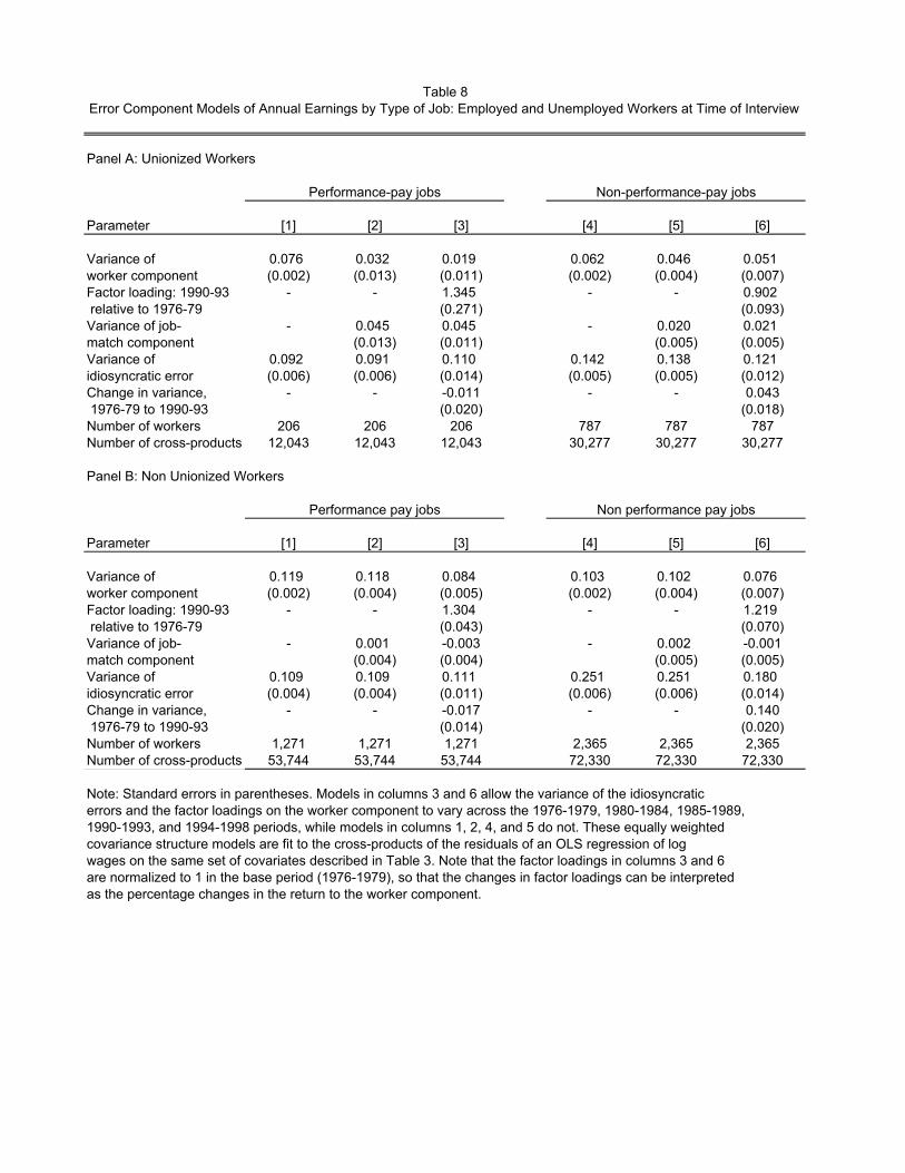
Panel A: Unionized Workers

Parameter [1] [2] [3] [4] [5] [6]


Panel B: Non Unionized Workers

Parameter [1] [2] [3] [4] [5] [6]

Variance of 0.119 0.118 0.084 0.103 0.102 0.076worker component (0.002) (0.004) (0.005) (0.002) (0.004) (0.007)Factor loading: 1990-93 - - 1.304 - - 1.219 relative to 1976-79 (0.043) (0.070)Variance of job- - 0.001 -0.003 - 0.002 -0.001match component (0.004) (0.004) (0.005) (0.005)Variance of 0.109 0.109 0.111 0.251 0.251 0.180idiosyncratic error (0.004) (0.004) (0.011) (0.006) (0.006) (0.014)Change in variance, - - -0.017 - - 0.140 1976-79 to 1990-93 (0.014) (0.020)Number of workers 1,271 1,271 1,271 2,365 2,365 2,365Number of cross-products 53,744 53,744 53,744 72,330 72,330 72,330



Table 8Error Component Models of Annual Earnings by Type of Job: Employed and Unemployed Workers at Time of Interview


Appendix Table 1

Empirical Covariance Matrix Residuals: Workers Employed at Interview Only

Panel A: Performance Pay Jobs

Log Hourly Earnings

Year1976 1977 1978 1979 1980 1981 1982 1983 1984 1985 1986 1987 1988 1989 1990 1991 1992 1993 1994 1995 1996 1998

1976 0.1981977 0.144 0.1771978 0.132 0.119 0.1791979 0.113 0.096 0.101 0.1761980 0.103 0.097 0.096 0.116 0.1631981 0.094 0.087 0.104 0.099 0.116 0.1711982 0.076 0.090 0.089 0.093 0.099 0.102 0.1731983 0.109 0.097 0.111 0.097 0.100 0.109 0.110 0.1631984 0.100 0.099 0.094 0.089 0.092 0.107 0.109 0.116 0.1841985 0.092 0.087 0.074 0.078 0.092 0.098 0.088 0.103 0.117 0.1811986 0.097 0.089 0.101 0.086 0.098 0.109 0.091 0.124 0.121 0.138 0.2111987 0.095 0.092 0.083 0.074 0.089 0.100 0.091 0.106 0.104 0.122 0.142 0.1831988 0.086 0.076 0.089 0.074 0.091 0.111 0.076 0.117 0.101 0.124 0.148 0.137 0.1901989 0.078 0.078 0.085 0.073 0.086 0.105 0.080 0.110 0.094 0.114 0.136 0.127 0.143 0.1771990 0.093 0.087 0.089 0.081 0.085 0.105 0.082 0.113 0.098 0.115 0.129 0.130 0.131 0.125 0.1761991 0.095 0.099 0.107 0.082 0.090 0.116 0.087 0.122 0.105 0.116 0.136 0.131 0.142 0.135 0.142 0.2111992 0.112 0.075 0.113 0.075 0.086 0.099 0.079 0.095 0.089 0.105 0.128 0.123 0.134 0.128 0.118 0.124 0.2511993 0.102 0.072 0.086 0.093 0.099 0.100 0.077 0.104 0.107 0.101 0.125 0.115 0.130 0.119 0.120 0.133 0.129 0.1931994 0.093 0.088 0.083 0.084 0.099 0.099 0.092 0.095 0.094 0.100 0.118 0.105 0.111 0.097 0.110 0.112 0.111 0.116 0.1881995 0.089 0.086 0.075 0.070 0.075 0.070 0.084 0.072 0.089 0.089 0.119 0.104 0.111 0.104 0.107 0.110 0.107 0.129 0.118 0.1961996 0.087 0.072 0.072 0.059 0.085 0.099 0.086 0.082 0.100 0.104 0.128 0.123 0.126 0.124 0.123 0.123 0.106 0.128 0.128 0.133 0.2271998 0.051 0.061 0.065 0.081 0.089 0.081 0.057 0.068 0.084 0.087 0.102 0.097 0.130 0.109 0.125 0.111 0.100 0.132 0.132 0.123 0.132 0.238

Log Annual Earnings

Year1976 1977 1978 1979 1980 1981 1982 1983 1984 1985 1986 1987 1988 1989 1990 1991 1992 1993 1994 1995 1996 1998

1976 0.2121977 0.133 0.1611978 0.116 0.117 0.1601979 0.116 0.104 0.110 0.1931980 0.097 0.095 0.091 0.133 0.1971981 0.094 0.089 0.100 0.107 0.129 0.1921982 0.091 0.099 0.087 0.102 0.114 0.128 0.2181983 0.109 0.108 0.109 0.104 0.107 0.108 0.120 0.2031984 0.109 0.110 0.099 0.105 0.106 0.117 0.128 0.136 0.2121985 0.090 0.101 0.080 0.094 0.105 0.104 0.104 0.117 0.136 0.1881986 0.092 0.110 0.095 0.096 0.113 0.119 0.103 0.138 0.142 0.161 0.2681987 0.090 0.108 0.084 0.086 0.092 0.108 0.099 0.111 0.115 0.129 0.156 0.2111988 0.093 0.092 0.096 0.089 0.098 0.118 0.097 0.116 0.112 0.133 0.156 0.144 0.2071989 0.092 0.090 0.086 0.105 0.108 0.118 0.091 0.113 0.103 0.126 0.150 0.135 0.147 0.2321990 0.091 0.092 0.090 0.097 0.093 0.107 0.087 0.113 0.105 0.115 0.129 0.136 0.143 0.146 0.2011991 0.099 0.106 0.103 0.102 0.091 0.115 0.089 0.118 0.112 0.120 0.139 0.140 0.146 0.149 0.162 0.2361992 0.105 0.083 0.089 0.089 0.094 0.105 0.080 0.100 0.095 0.106 0.138 0.130 0.153 0.134 0.131 0.149 0.2151993 0.112 0.093 0.073 0.087 0.085 0.094 0.072 0.094 0.101 0.101 0.122 0.119 0.139 0.131 0.136 0.135 0.145 0.2041994 0.097 0.086 0.082 0.088 0.103 0.105 0.099 0.099 0.100 0.106 0.117 0.109 0.130 0.101 0.121 0.118 0.124 0.137 0.2131995 0.082 0.069 0.063 0.067 0.061 0.072 0.083 0.084 0.082 0.081 0.105 0.087 0.110 0.106 0.110 0.119 0.105 0.133 0.130 0.2131996 0.088 0.083 0.075 0.056 0.083 0.111 0.102 0.107 0.099 0.107 0.127 0.124 0.145 0.154 0.132 0.129 0.117 0.137 0.131 0.143 0.2311998 0.053 0.058 0.063 0.067 0.075 0.079 0.055 0.072 0.058 0.084 0.098 0.088 0.120 0.110 0.120 0.106 0.101 0.139 0.137 0.127 0.150 0.234

42

Panel B: Non Performance Pay Jobs

Log Hourly Earnings

Year1976 1977 1978 1979 1980 1981 1982 1983 1984 1985 1986 1987 1988 1989 1990 1991 1992 1993 1994 1995 1996 1998

1976 0.1541977 0.093 0.1251978 0.080 0.083 0.1661979 0.071 0.074 0.096 0.1621980 0.073 0.074 0.092 0.094 0.1461981 0.072 0.068 0.084 0.083 0.095 0.1561982 0.060 0.069 0.076 0.076 0.088 0.097 0.1641983 0.055 0.058 0.065 0.062 0.076 0.078 0.089 0.1371984 0.058 0.056 0.061 0.060 0.071 0.077 0.080 0.076 0.1561985 0.047 0.047 0.058 0.063 0.080 0.082 0.085 0.071 0.083 0.1611986 0.050 0.050 0.047 0.054 0.061 0.072 0.073 0.074 0.078 0.097 0.1461987 0.053 0.047 0.049 0.052 0.068 0.065 0.069 0.060 0.064 0.092 0.080 0.1531988 0.045 0.051 0.044 0.035 0.060 0.059 0.070 0.068 0.072 0.088 0.087 0.088 0.1671989 0.042 0.038 0.043 0.034 0.051 0.053 0.054 0.056 0.061 0.080 0.069 0.079 0.099 0.1431990 0.050 0.046 0.047 0.046 0.048 0.056 0.063 0.070 0.073 0.079 0.078 0.081 0.100 0.108 0.1621991 0.046 0.037 0.035 0.037 0.045 0.053 0.062 0.065 0.064 0.073 0.072 0.067 0.090 0.090 0.100 0.1541992 0.041 0.027 0.023 0.021 0.037 0.053 0.048 0.068 0.049 0.059 0.065 0.061 0.077 0.082 0.086 0.082 0.2211993 0.041 0.042 0.035 0.040 0.041 0.055 0.059 0.087 0.059 0.071 0.072 0.067 0.083 0.075 0.091 0.097 0.074 0.2411994 0.030 0.033 0.027 0.026 0.037 0.049 0.044 0.068 0.041 0.068 0.062 0.060 0.069 0.070 0.069 0.074 0.075 0.090 0.1991995 0.043 0.028 0.024 0.024 0.045 0.039 0.028 0.049 0.043 0.051 0.052 0.052 0.059 0.067 0.069 0.074 0.064 0.081 0.091 0.1731996 0.031 0.025 0.014 0.025 0.041 0.049 0.046 0.061 0.045 0.056 0.066 0.059 0.057 0.051 0.058 0.078 0.078 0.078 0.078 0.095 0.1921998 0.054 0.026 0.023 0.018 0.033 0.045 0.019 0.055 0.049 0.055 0.060 0.063 0.072 0.065 0.064 0.094 0.076 0.098 0.092 0.090 0.102 0.205

Log Annual Earnings

Year1976 1977 1978 1979 1980 1981 1982 1983 1984 1985 1986 1987 1988 1989 1990 1991 1992 1993 1994 1995 1996 1998

1976 0.1981977 0.114 0.1931978 0.085 0.109 0.1951979 0.093 0.115 0.120 0.2151980 0.089 0.110 0.122 0.127 0.2281981 0.084 0.103 0.103 0.113 0.131 0.2281982 0.071 0.084 0.085 0.094 0.117 0.124 0.2421983 0.070 0.083 0.079 0.089 0.100 0.104 0.112 0.2431984 0.063 0.074 0.069 0.081 0.093 0.092 0.097 0.108 0.2281985 0.066 0.067 0.064 0.082 0.095 0.096 0.097 0.098 0.107 0.2571986 0.071 0.066 0.055 0.076 0.079 0.082 0.096 0.100 0.102 0.127 0.2361987 0.086 0.086 0.070 0.080 0.088 0.093 0.093 0.091 0.107 0.122 0.120 0.2641988 0.062 0.069 0.048 0.066 0.067 0.070 0.076 0.097 0.089 0.094 0.103 0.122 0.2471989 0.054 0.066 0.066 0.051 0.063 0.057 0.073 0.067 0.076 0.094 0.108 0.131 0.114 0.2661990 0.046 0.064 0.062 0.053 0.066 0.069 0.084 0.100 0.093 0.098 0.109 0.117 0.126 0.183 0.3841991 0.047 0.058 0.040 0.049 0.061 0.059 0.088 0.083 0.071 0.088 0.093 0.096 0.106 0.101 0.128 0.2271992 0.028 0.041 0.024 0.044 0.066 0.063 0.064 0.078 0.062 0.075 0.089 0.095 0.097 0.093 0.116 0.119 0.2761993 0.046 0.060 0.045 0.055 0.074 0.067 0.063 0.084 0.069 0.077 0.084 0.094 0.079 0.088 0.113 0.108 0.117 0.3101994 0.028 0.026 0.012 0.034 0.057 0.056 0.054 0.071 0.051 0.093 0.082 0.093 0.075 0.079 0.088 0.092 0.115 0.130 0.3041995 0.038 0.043 0.040 0.040 0.065 0.050 0.064 0.054 0.063 0.072 0.062 0.071 0.067 0.064 0.090 0.086 0.072 0.098 0.122 0.2431996 0.032 0.036 0.041 0.046 0.045 0.063 0.073 0.059 0.049 0.067 0.081 0.073 0.063 0.056 0.070 0.085 0.086 0.086 0.096 0.113 0.2341998 0.055 0.033 0.024 0.034 0.027 0.043 0.048 0.079 0.087 0.058 0.062 0.057 0.065 0.060 0.077 0.087 0.098 0.099 0.082 0.086 0.103 0.232

43

Order of [1] [2] [3] [4]autocov: Wage Earnings Wage Earnings

0 0.191 0.209 0.167 0.2481 0.124 0.138 0.091 0.1222 0.119 0.127 0.085 0.1093 0.115 0.122 0.078 0.0984 0.108 0.116 0.074 0.0925 0.109 0.115 0.072 0.0886 0.102 0.111 0.066 0.0807 0.103 0.109 0.062 0.0778 0.101 0.105 0.057 0.0699 0.098 0.102 0.055 0.07110 0.095 0.098 0.053 0.06611 0.090 0.092 0.053 0.06512 0.089 0.094 0.046 0.05913 0.089 0.093 0.042 0.05714 0.092 0.089 0.040 0.05615 0.083 0.084 0.040 0.05316 0.080 0.081 0.032 0.03917 0.081 0.079 0.034 0.04018 0.085 0.079 0.026 0.03519 0.081 0.077 0.028 0.03620 0.076 0.076 0.027 0.02822 0.051 0.053 0.054 0.055

Appendix Table 2: Autocovariances in Wages and Earnings(workers employed or unemployed at the time of the interview)

Performance-pay Non-Performance-Pay

Empirical Covariance Matrix of Residuals: Workers Employed or Unemployed at Interview

Panel A: Performance Pay Jobs

Log Hourly Earnings

Year1976 1977 1978 1979 1980 1981 1982 1983 1984 1985 1986 1987 1988 1989 1990 1991 1992 1993 1994 1995 1996 1998

1976 0.1961977 0.143 0.1741978 0.137 0.120 0.1861979 0.113 0.096 0.102 0.1921980 0.105 0.096 0.103 0.114 0.1671981 0.096 0.085 0.106 0.099 0.111 0.1681982 0.078 0.089 0.089 0.093 0.097 0.103 0.1771983 0.110 0.095 0.112 0.096 0.099 0.110 0.110 0.1631984 0.101 0.100 0.095 0.088 0.091 0.106 0.108 0.112 0.1821985 0.088 0.080 0.069 0.080 0.088 0.098 0.088 0.099 0.114 0.1801986 0.096 0.088 0.102 0.085 0.099 0.108 0.094 0.125 0.124 0.136 0.2151987 0.094 0.087 0.082 0.071 0.084 0.095 0.088 0.103 0.104 0.121 0.142 0.1901988 0.087 0.076 0.090 0.074 0.089 0.106 0.075 0.113 0.101 0.122 0.146 0.137 0.1911989 0.077 0.076 0.084 0.072 0.084 0.101 0.078 0.106 0.093 0.112 0.134 0.127 0.141 0.1761990 0.091 0.083 0.088 0.078 0.083 0.101 0.081 0.111 0.096 0.112 0.126 0.131 0.131 0.126 0.1811991 0.091 0.095 0.104 0.081 0.090 0.111 0.083 0.117 0.104 0.115 0.137 0.129 0.139 0.134 0.140 0.2131992 0.107 0.069 0.110 0.072 0.084 0.095 0.079 0.093 0.086 0.103 0.126 0.123 0.134 0.127 0.116 0.124 0.2521993 0.098 0.067 0.084 0.088 0.096 0.095 0.073 0.100 0.104 0.099 0.126 0.118 0.128 0.119 0.118 0.134 0.126 0.1911994 0.084 0.079 0.078 0.080 0.092 0.091 0.083 0.090 0.088 0.101 0.117 0.108 0.110 0.096 0.105 0.108 0.106 0.112 0.1941995 0.087 0.076 0.074 0.068 0.073 0.069 0.081 0.071 0.088 0.088 0.118 0.106 0.110 0.103 0.108 0.111 0.106 0.126 0.116 0.1941996 0.085 0.069 0.071 0.056 0.083 0.096 0.083 0.080 0.099 0.104 0.130 0.124 0.125 0.123 0.128 0.127 0.113 0.129 0.125 0.132 0.2291998 0.050 0.057 0.065 0.077 0.087 0.082 0.060 0.068 0.083 0.087 0.103 0.101 0.127 0.110 0.125 0.109 0.102 0.131 0.129 0.123 0.131 0.237

Log Annual Earnings

Year1976 1977 1978 1979 1980 1981 1982 1983 1984 1985 1986 1987 1988 1989 1990 1991 1992 1993 1994 1995 1996 1998

1976 0.2171977 0.139 0.1731978 0.118 0.119 0.1721979 0.115 0.104 0.110 0.1991980 0.097 0.096 0.096 0.133 0.2041981 0.098 0.097 0.109 0.109 0.126 0.2091982 0.092 0.105 0.090 0.102 0.114 0.141 0.2361983 0.110 0.111 0.111 0.105 0.109 0.121 0.124 0.2441984 0.108 0.110 0.105 0.103 0.106 0.119 0.130 0.135 0.2121985 0.087 0.097 0.076 0.092 0.101 0.101 0.104 0.115 0.133 0.1981986 0.092 0.108 0.097 0.085 0.113 0.119 0.105 0.138 0.144 0.161 0.2821987 0.091 0.110 0.084 0.085 0.088 0.110 0.103 0.111 0.117 0.130 0.154 0.2231988 0.095 0.092 0.094 0.082 0.096 0.109 0.097 0.116 0.112 0.126 0.151 0.141 0.2181989 0.091 0.091 0.084 0.103 0.103 0.109 0.091 0.110 0.103 0.127 0.148 0.136 0.146 0.2331990 0.087 0.090 0.087 0.092 0.089 0.107 0.090 0.115 0.102 0.112 0.126 0.139 0.142 0.146 0.2091991 0.096 0.102 0.098 0.096 0.097 0.119 0.091 0.118 0.109 0.120 0.139 0.138 0.144 0.153 0.158 0.2611992 0.103 0.083 0.088 0.087 0.093 0.103 0.082 0.104 0.096 0.110 0.136 0.129 0.153 0.136 0.130 0.149 0.2171993 0.108 0.087 0.075 0.086 0.081 0.088 0.068 0.092 0.098 0.100 0.120 0.125 0.138 0.135 0.139 0.138 0.144 0.2151994 0.088 0.081 0.078 0.085 0.094 0.103 0.094 0.098 0.094 0.107 0.116 0.113 0.128 0.103 0.121 0.115 0.121 0.135 0.2291995 0.079 0.070 0.062 0.064 0.059 0.075 0.091 0.086 0.079 0.080 0.103 0.087 0.107 0.104 0.112 0.118 0.103 0.133 0.128 0.2111996 0.085 0.080 0.073 0.053 0.080 0.104 0.100 0.107 0.098 0.104 0.126 0.121 0.138 0.150 0.135 0.129 0.121 0.135 0.129 0.141 0.2301998 0.050 0.054 0.061 0.064 0.073 0.079 0.057 0.072 0.057 0.083 0.099 0.089 0.117 0.107 0.120 0.111 0.103 0.136 0.135 0.127 0.149 0.235

Appendix Table 3

Panel B: Non Performance Pay Jobs

Log Hourly Earnings

Year1976 1977 1978 1979 1980 1981 1982 1983 1984 1985 1986 1987 1988 1989 1990 1991 1992 1993 1994 1995 1996 1998

1976 0.1631977 0.093 0.1301978 0.080 0.078 0.1721979 0.069 0.072 0.099 0.1651980 0.073 0.070 0.087 0.092 0.1631981 0.067 0.063 0.072 0.072 0.100 0.1711982 0.059 0.065 0.074 0.071 0.089 0.101 0.1781983 0.053 0.057 0.067 0.066 0.075 0.079 0.089 0.1491984 0.054 0.054 0.062 0.063 0.069 0.083 0.082 0.078 0.1691985 0.048 0.046 0.065 0.067 0.073 0.079 0.091 0.075 0.087 0.1771986 0.049 0.050 0.048 0.058 0.060 0.075 0.078 0.072 0.076 0.100 0.1681987 0.051 0.045 0.053 0.055 0.067 0.068 0.072 0.065 0.066 0.087 0.080 0.1631988 0.043 0.046 0.045 0.035 0.049 0.055 0.072 0.067 0.069 0.087 0.085 0.085 0.1761989 0.044 0.038 0.042 0.033 0.048 0.046 0.053 0.056 0.058 0.074 0.071 0.075 0.097 0.1531990 0.041 0.046 0.048 0.043 0.043 0.053 0.070 0.070 0.071 0.084 0.073 0.077 0.093 0.105 0.1691991 0.040 0.032 0.032 0.035 0.041 0.048 0.063 0.063 0.062 0.070 0.067 0.067 0.088 0.089 0.095 0.1621992 0.036 0.032 0.014 0.034 0.040 0.048 0.058 0.069 0.052 0.057 0.055 0.059 0.070 0.068 0.082 0.072 0.2551993 0.038 0.043 0.029 0.044 0.048 0.046 0.061 0.089 0.064 0.076 0.069 0.071 0.081 0.075 0.087 0.102 0.076 0.2601994 0.029 0.029 0.025 0.030 0.045 0.044 0.047 0.070 0.045 0.070 0.071 0.066 0.067 0.068 0.071 0.073 0.075 0.095 0.2071995 0.040 0.021 0.022 0.022 0.037 0.028 0.027 0.051 0.042 0.047 0.050 0.051 0.055 0.066 0.062 0.066 0.058 0.081 0.088 0.1741996 0.025 0.021 0.013 0.026 0.044 0.044 0.047 0.063 0.054 0.056 0.067 0.062 0.056 0.052 0.056 0.077 0.076 0.086 0.076 0.095 0.2021998 0.052 0.023 0.018 0.020 0.046 0.048 0.018 0.062 0.047 0.053 0.057 0.065 0.071 0.063 0.061 0.089 0.071 0.105 0.089 0.088 0.101 0.209

Log Annual Earnings

Year1976 1977 1978 1979 1980 1981 1982 1983 1984 1985 1986 1987 1988 1989 1990 1991 1992 1993 1994 1995 1996 1998

1976 0.2311977 0.128 0.2381978 0.086 0.109 0.2341979 0.093 0.113 0.130 0.2591980 0.081 0.100 0.129 0.139 0.2751981 0.085 0.093 0.096 0.105 0.136 0.3451982 0.077 0.082 0.085 0.087 0.111 0.174 0.3531983 0.064 0.074 0.085 0.081 0.108 0.105 0.147 0.3351984 0.053 0.078 0.082 0.079 0.111 0.120 0.137 0.124 0.3761985 0.076 0.077 0.091 0.085 0.093 0.104 0.128 0.110 0.135 0.3491986 0.065 0.068 0.064 0.077 0.080 0.117 0.105 0.091 0.123 0.156 0.3301987 0.084 0.109 0.072 0.092 0.082 0.109 0.113 0.080 0.108 0.152 0.146 0.3831988 0.059 0.073 0.046 0.066 0.063 0.082 0.108 0.092 0.098 0.089 0.113 0.137 0.3411989 0.056 0.074 0.047 0.052 0.055 0.098 0.096 0.065 0.084 0.091 0.101 0.135 0.130 0.3001990 0.053 0.070 0.044 0.050 0.093 0.137 0.145 0.096 0.150 0.099 0.113 0.136 0.140 0.210 0.4501991 0.051 0.063 0.045 0.044 0.079 0.079 0.090 0.079 0.081 0.103 0.096 0.093 0.123 0.114 0.138 0.3191992 0.027 0.085 0.029 0.053 0.061 0.044 0.066 0.076 0.097 0.063 0.093 0.095 0.077 0.083 0.136 0.112 0.4251993 0.037 0.051 0.039 0.043 0.067 0.064 0.055 0.074 0.077 0.088 0.089 0.096 0.086 0.086 0.109 0.107 0.112 0.3671994 0.016 0.068 0.015 0.034 0.037 0.046 0.058 0.064 0.065 0.102 0.103 0.113 0.078 0.074 0.100 0.115 0.115 0.121 0.3441995 0.028 0.039 0.042 0.034 0.042 0.028 0.070 0.067 0.076 0.093 0.059 0.067 0.067 0.059 0.078 0.072 0.069 0.091 0.122 0.2531996 0.016 0.060 0.040 0.056 0.052 0.070 0.060 0.058 0.052 0.085 0.077 0.070 0.062 0.068 0.073 0.079 0.087 0.099 0.092 0.111 0.2541998 0.028 0.047 0.031 0.043 0.056 0.038 0.045 0.078 0.090 0.065 0.068 0.066 0.070 0.059 0.086 0.084 0.099 0.103 0.079 0.083 0.103 0.234

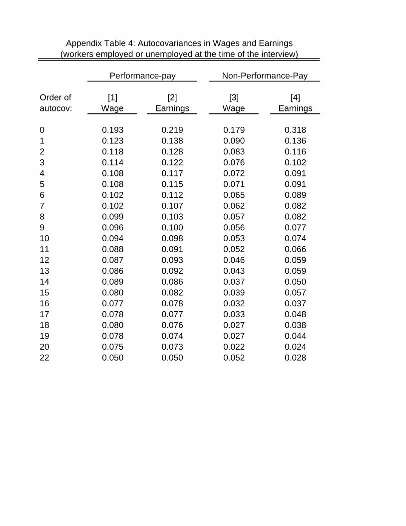
Order of [1] [2] [3] [4]autocov: Wage Earnings Wage Earnings

0 0.193 0.219 0.179 0.3181 0.123 0.138 0.090 0.1362 0.118 0.128 0.083 0.1163 0.114 0.122 0.076 0.1024 0.108 0.117 0.072 0.0915 0.108 0.115 0.071 0.0916 0.102 0.112 0.065 0.0897 0.102 0.107 0.062 0.0828 0.099 0.103 0.057 0.0829 0.096 0.100 0.056 0.07710 0.094 0.098 0.053 0.07411 0.088 0.091 0.052 0.06612 0.087 0.093 0.046 0.05913 0.086 0.092 0.043 0.05914 0.089 0.086 0.037 0.05015 0.080 0.082 0.039 0.05716 0.077 0.078 0.032 0.03717 0.078 0.077 0.033 0.04818 0.080 0.076 0.027 0.03819 0.078 0.074 0.027 0.04420 0.075 0.073 0.022 0.02422 0.050 0.050 0.052 0.028

Appendix Table 4: Autocovariances in Wages and Earnings(workers employed or unemployed at the time of the interview)

Performance-pay Non-Performance-Pay

performance pay and the autocovariance structure of

Documents