performance of emerging technologies for measuring solid

Performance of Emerging Technologies for Measuring Solid and LiquidPrecipitation in Cold Climate as Compared to the Traditional Manual Gauges

FAISAL S. BOUDALA

Cloud Physics and Severe Weather Research Section, Environment and Climate Change Canada, Toronto,

Ontario, Canada

GEORGE A. ISAAC

Weather Impacts Consulting Inc., Barrie, Ontario, Canada

PETER FILMAN

Department of National Defence, Government of Canada, Cold Lake, Alberta, Canada

ROBERT CRAWFORD AND DAVID HUDAK

Cloud Physics and Severe Weather Research Section, Environment and Climate Change Canada,

Toronto, Ontario, Canada

MARTHA ANDERSON

Department of National Defence, Government of Canada, Ottawa, Ontario, Canada

(Manuscript received 26 April 2016, in final form 7 September 2016)

ABSTRACT

Precipitation amount, type, and snow depth (Ds) have been analyzed using data collected during the 4WingCold

LakeResearch Project in northeasternAlberta, Canada. The instruments used include theVaisala present weather

detector PWD22 and present weather sensor (FS)11P, the OTT Pluvio2 automatic catchment-type gauge, the

manual standard Canadian Nipher (CN) and Type B rain gauges, and a snow ruler. Both the PWD22 and FS11P

performed well at detecting snow, rain, and drizzle events as compared to the human observer. The sensors

predicted a higher frequency of ice pellet cases than the human observer. Segregation of precipitation phase using

temperature alone appeared unrealistic at near-freezing temperatures. All the sensors agreed well at measuring

liquid precipitation, but the Pluvio2 gauge with a single Alter shield underestimated the snowfall amount by 40%,

mostly due to wind effects. After correcting the CN gauge catch efficiency (CE) due to wind effects, the CE of the

Pluvio2 relative to theCNgaugewas founddependent onwind speed (ws).Using these data, a new transfer function

(TF) for the Pluvio2 as a function ofws has been developed. The newTFwas used to correct the Pluvio2 gauge, and

the corrected data agreed well with the PWD22measurements. Using theDs and corrected CN data, snow density

ratios (ry) were derived, varying from 4.2 to 35 with a mean value of 12.2. The mean value derived in this study is

higher than the 10:1 ratio usually assumed for converting Ds to snow water equivalent in Canada. On average ryincreases with increasing temperature and the 10:1 ratio appears to be more appropriate for warmer temperatures.

1. Introduction

Precipitation plays a critical role on our planet by

modulating the hydrological cycle and by influencing daily

human activities, including air and ground transportation.

Validation of climate and numerical weather prediction

models, and radar and satellite remote sensing algorithms,

require accurate precipitationmeasurements. Precipitation

amount is normally measured using a weighing gauge,

which is an open container on the ground that collects

precipitating hydrometeors, including raindrops, snow and

Publisher’s Note:This article was revised on 3March 2017 in order

to correct the affiliations of the last three authors.

Corresponding author e-mail: Dr. Faisal Boudala, faisal.boudala@

canada.ca

JANUARY 2017 BOUDALA ET AL . 167

DOI: 10.1175/JTECH-D-16-0088.1

� 2017 American Meteorological Society

mailto:[email protected]

mailto:[email protected]

hail particles, etc. However, accurately measuring the

precipitation is usuallymore complex, particularly for snow

because of many factors, including losses from wind, wet-

ting, and evaporation (Sevruk and Klemm 1989; Goodison

et al. 1998; Rasmussen et al. 2012; Yang et al. 2005) and

potential enhancement due to blowing snow (Yang et al.

1999). Recent studies also indicate that snow gauge catch

efficiency depends on snow type and density (Thériaultet al. 2015, 2012; Colli et al. 2015, 2016a,b). This is partic-

ularly challenging in the cold northern latitudes, where the

snowfall intensities are relatively low. The manual gauges

that are deployed in the Canadian precipitation networks

include the Type B and Canadian Nipher (Mekis and

Vincent 2011; Metcalfe and Goodison 1993). These

gauges are normally referred to as standard rain gauges.

Automatic gauges, such as Geonor and Pluvio, are cur-

rently being considered for the networks.

One way to reduce the wind-induced loss is by using

some kind of wind shield, by placing a given gauge inside

some bushes, or using specially designed shields, including

the double-fenced structure with a Tretyakov manual

gauge suggested by the World Meteorological Organiza-

tion (WMO), which is normally referred to as Double

Fence IntercomparisonReference (DFIR) (Goodison et al.

1998). There is no absolute reference standard for snow

measurement. The DFIR is usually considered the sec-

ondary standard with the bush-surrounded gauge being the

primary standard (Goodison et al. 1998;Yang 2014). Part of

the reason why the bush gauge is considered to be the

primary standard is because it showed higher catch effi-

ciency as compared to the gauge placed inside the DFIR

(Goodison et al. 1998).Amore recent studybyYang (2014)

showed that the DFIR underestimated solid precipitation

by 5% as compared to the bush gauge. During the WMO

Solid PrecipitationMeasurement Intercomparison (SPMI),

the Canadian Nipher gauge outperformed many other

partially shielded or unshielded gauges when compared

against a Russian Tretyakov manual gauge as the DFIR

(Goodison et al. 1998). One of the outcomes of the WMO

SPMI was the development of correction factors for un-

shielded and partially shielded gauges that are normally

referred to as transfer functions (Goodison et al. 1998).

These transfer functions were developed based on daily

manual snow measurements, and so there are some un-

certainties with their use at shorter time scales due to the

strong variability normally seen during precipitation and

associated weather conditions. These automatic gauges are

currently being used with various wind shield configura-

tions, including the double-fenced structure suggested by

the WMO, but their accuracy under various atmospheric

conditions are not well known (Rasmussen et al. 2012;

Theriault et al. 2015), particularly for the light solid pre-

cipitation that normally occurs in cold climates. There are

also noncatchment-type optical instruments that employ a

forward light scattering method, and hot plates and dis-

trometers that measure hydrometer size and fall velocity

distributions to estimate the precipitation intensities

(Rasmussen et al. 2011; Boudala et al. 2014a,b; Brandes

et al. 2007). These emerging technologies usually are more

sensitive and measure precipitation intensity at higher

temporal resolution down to minutes. Some of these in-

struments do not suffer from the wind-induced and other

losses mentioned earlier and hence are suitable for mea-

suring particularly light precipitation. However, these in-

struments are relatively new and their response under

various atmospheric conditions is not well known.

This study aims to address some of the issues associated

with both catchment- and noncatchment-type gauges, in-

cluding testing their performance under a cold climate,

providing suitable guidance to improve the accuracy of the

catchment-type gauges, and characterize snow density

under various weather conditions. For this purpose, pre-

cipitation and type, and snow depth data were collected

and analyzed as part of the 4Wing Cold Lake Research

Project (4WCLRP). Various instruments were used, in-

cluding the Vaisala present weather sensors PWD22 and

FS11P, the OTT Pluvio2 gauge, the Canadian Nipher and

Type Bmanual gauges, and a snow ruler to measure snow

depth. The 4WCLRP was initiated by the Cloud Physics

and Severe Weather Research Section of Environment

and Climate Change Canada (ECCC) with the co-

operation of theDepartment ofNationalDefence (DND).

The data used in this study were collected during the pe-

riod between September 2014 andAugust 2015. The paper

is organized as follows: The observation site and in-

strumentation are discussed in section 2, the precipitation

amount and type data analysis and results are given in

section 3, the snow density is discussed in section 4, and the

summary and conclusions are given in section 5.

2. Observation sites and instrumentation

The study area, the Cold Lake Regional Airport

(CYOD), is located in northeastern Alberta, Canada

(at 541m MSL; 54823059.800N, 11081706.200W). The geo-

graphical locations of CYOD (Fig. 1a) and the surround-

ing areas, and inside COYD where the instruments were

located (Figs. 1a,b) are shown. In Fig. 1b, in addition to the

ECCC observation site used in this study, there is a col-

located permanent meteorological observation site used

by the DND. The region is generally characterized by a

humid continental climate with warm summers and cold

winters as indicated in Fig. 2, which shows monthly aver-

aged temperature (Fig. 2a), relative humidity (Fig. 2b), and

the frequency distributions for temperature and humidity

(Figs. 2c,d, respectively) based on hourly observations

168 JOURNAL OF ATMOSPHER IC AND OCEAN IC TECHNOLOGY VOLUME 34

taken during the 2014–15 period. The monthly mean

temperature varies from 2128C in January to 188C in

July. Theminimum temperature in winter reached near

2358C, the warmest temperature is close to 278C in

summer, and the most frequent temperature is close to

08C (Fig. 2c). The monthly averaged humidity varied

from 85% in winter (December) to near 55% in sum-

mer (May). The humidity may reach as low as 15% in

April and May, but within a given month the humidity

may reach 100%, and the most frequent humidity is

90% (Fig. 2d). As indicated in Fig. 1a, there are a

number of local conditions that can potentially affect the

local weather and produce precipitation. To the west and

northwest of the airport, there are four small lakes (Marie,

Ethel, Crane, and Hilda) and to the northeast there are

two large lakes (Cold and Primrose) known to produce

precipitation and other weather phenomena when the

flow is from a northeasterly direction. The west and

southwest sides of the airport are surrounded by the

Beaver River valley with an east–west orientation,

FIG. 1. Google map showing (a) Cold Lake and surrounding areas and (b) two instrument sites. In (b) the site

marked as ECC is where the ECCC instruments were located, and the site marked as DND is where the DND

permanent observing site is located.


which is also known to produce various weather con-

ditions at the airport.

The list of the deployed instruments along with the

measured microphysical and meteorological parame-

ters, measurement principles, and associated uncer-

tainties are given in Table 1. The instrument setup at the

ECCC site is given in the top panel of Fig. 3, and the

instruments installed at the DND site are given in

Figs. 3a,b. The DND observation site is located ap-

proximately 948m from the ECCC site. The descrip-

tions and measurement principles of the instruments

installed at the ECCC and DND sites are given below.

The Vaisala PWD22 and FS11P present weather

sensors measure precipitation, precipitation type, and

visibility. The operating principles of these two Vaisala

sensors are similar with some minor differences (Table

1). These probes have two arms facing each other, one

equipped with a near-infrared transmitter and the other

with a receiver. The two arms are arranged in a way that

the infrared light can reach the receiver only if it is

forward scattered at a given angle (458 for PWD22 and

428 for FS11P) by particles between the arms. Signal

processing software analyzes the voltage output from

the receiver, along with the current temperature, to

determine the type and intensity of precipitation. The

reported precipitation types include the WMO synoptic

(SYNOP) and METAR codes, as well as the National

Weather Service (NWS) code. Each instrument also

has a heated capacitive surface that provides a liquid

water equivalent measurement. The FS11P is also

equipped with a background light detection sensor.

The OTT Pluvio2 precipitation gauge used here has a

precipitation-collecting container with a collecting area

of 200 cm2 and a capacity of up to 1500mm. The weight

of the precipitation collected in the container is mea-

sured every 6 s by an electronic weighing cell at a reso-

lution of 0.01mm. The measured precipitation intensity

and amount are reported everyminute. TheOTTPluvio2

uses a special filter algorithm to correct the 6-s pre-

cipitation weights for wind effects. Additionally, the

gauge is fitted with a single Alter shield, as shown in

Fig. 3a, to minimize the wind effect during snow (see

Table 1 for more information). The OTT Pluvio2, ver-

sion 200, is also supplied with an orifice rim heating

system. This reliably keeps the orifice ring rim free of

snow and ice during low-temperature operations.

The Vaisala weather transmitter (WXT) 520 mea-

sures temperature, relative humidity, and wind speed

and direction. The wind sensor has an array of equally

spaced ultrasonic transducers on a horizontal plane.

The wind speed and direction are determined by

measuring the time it takes the ultrasound to travel

from one transducer to the other. The instrument uses

separate sensors for measuring temperature and rela-

tive humidity. The accuracy and resolution of these

measurements are given in Table 1.

The manual gauges used for measuring the total

precipitation and rain amounts are the Type B and

Canadian Nipher gauges shown in Fig. 3b. The Type B

and Nipher gauges are the standard instruments for

rain and snow observations, respectively, in Canada

(Mekis and Vincent 2011; Metcalfe and Goodison

1993). The snow amount in its water equivalent form

is determined using the Canadian Nipher gauge. The

falling snow is collected and melted and then measured

bypouring it into a graduated cylinder. The rainfall amount

FIG. 2. Climatology of Cold Lake based on 2 years of hourly reported data.


TABLE1.ThedescriptionoftheinstrumentsinstalledatCYOD

andrelatedinform

ation.

InstrumentName

Model

Sensortype

Parameter

measured

Range

Resolution

Accuracy

Data

recorded

Capacitance

RH

0%

to100%

0.47

60.8%

at238C

10s

Vaisalaweather

transm

itter

WXT520

Ultrasonic

transducers

Windspeed

0–60m

s21

0.1m

s21

60.3m

s21(0–35m

s21)

1min

5%

(36–60m

s21)

Ultrasonic

transducers

Wind

direction

0–360

18

638

1min

Capacitiveceramic

THERMOCAP

T2528–608C

0.18C

60.38C

1min

Capacitivethin-film

HUMIC

AP

RH

0%

–100%

0.1%

63%

(0%–90%)

1min

65%

(90%–100%

)

Vaisalapresent

weatherdetector

PW

D22

Forw

ard

scattered(458)

lightdetector(photo

diode),

lightsourcenear-IR

875nm

Visibility

10–20

000m

610%,10–10

000m

1min

615%,10–20km

Precipitation

intensity

and

type

—0.01mm

h21

—1min

Vaisalapresent

weathersensor

FS11P

Forw

ard

scattered(428)

lightdetector(photo

diode)

Lightsourcenear-IR

875nm

Visibility

5–75m

610%,5–10m

1min

620%,10–75km

Precipitation

intensity

andtype

—0.01mm

h21

—1min

OTTPluvio

gauge

Pluvio2,version200;

1500-mm

capacity

Stainless

steelload

cell-w

eighingsystem

Precipitation

amount

0.20–500mm

0.01mm

60.1mm

1min


ismeasured using theTypeB rain gauge. Inside theTypeB

gauge, there is a graduated cylinder that holds up to 25mm

of rain. Rainfall of more than 25mm can be made by

measuring the overflow of the cylinder into the surround-

ing container. The manually measured data were collected

every 6 h and segregated as solid, mixed, and liquid

phases. More details about how the precipitation phase

was segregated are given in section 3. As well the

depths of snow accumulated over aWeaver snow board

were measured by taking the average of 10 snow ruler

measurements in an undisturbed area around the me-

teorological compound.

3. Data analysis and results

a. Frequency distribution of precipitation type basedon 1-min data

Figure 4 shows the frequency distribution of pre-

cipitation type (PT) reported by the PWD22 and FS11P

present weather sensors based on 1-min data between

September 2014 and August 2015. The weather symbols

shown in Fig. 4 and Table 2 are C, S, SP, IP, SG, IC, R,

ZR, ZL, P, RLS, L, and RL represent clear, snow, snow

pellets, ice pellets, snow grains, ice crystals, rain, freez-

ing rain, freezing drizzle, unknown, mixed, drizzle, and

FIG. 3. (top) The ECCC instrument setup at CYOD. (a) The Type B and (b) the Canadian

Nipher manual gauges at the DND site.


rain and drizzle, respectively.When no precipitation was

reported (;88% of the time) or the clear case, the

PWD22 agreed well with the FS11P. Based on the

PWD22 and FS11P sensors, the frequency of pre-

cipitation events during the entire measurement period

was quite low, only 12%. Most of the reported pre-

cipitation types were snow with a frequency of 8% and

followed by rain 3%. There were only a few cases of L

and IP reported (see Fig. 4).

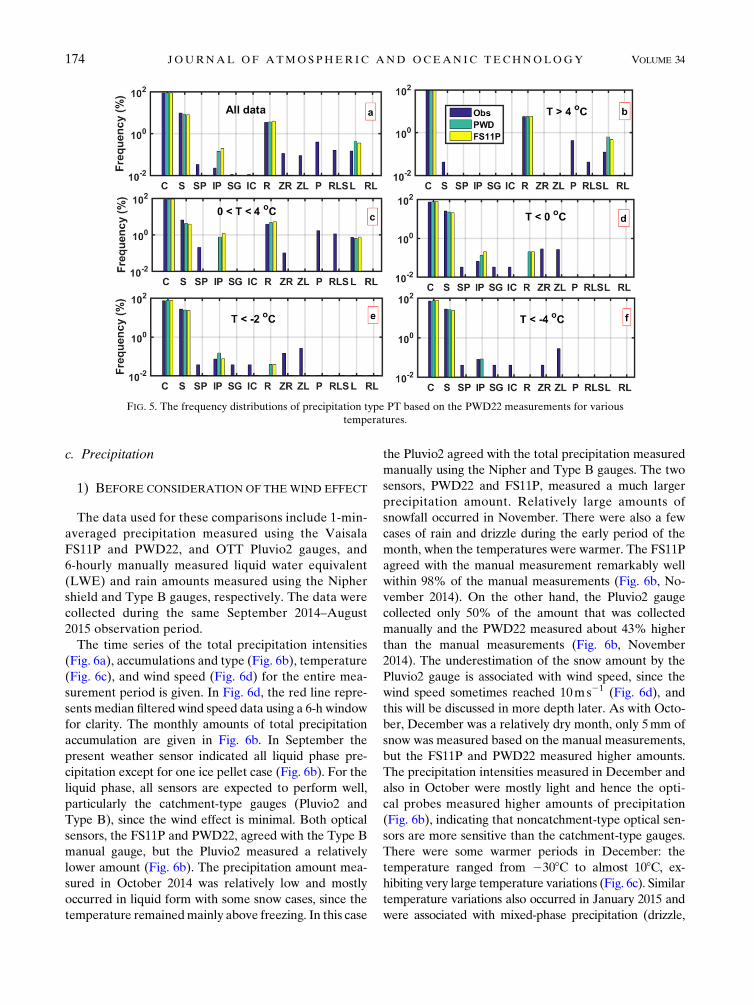
b. Frequency distribution of precipitation typecompared with human observer

For this comparison hourly data collected during the

same period mentioned in section 3a were used. From

the present weather sensors, hourly precipitation type

reports were extracted by using the nearest to human

observer time via an interpolation method. It is cus-

tomary to segregate precipitation phases using temper-

ature; for example, Rasmussen et al. (2011) assumed

precipitation phase as solid for (T , 08C), liquid for

(T. 48C), andmixed for other temperatures. To test such

assumptions, the hourly precipitation type frequency

data were also segregated based on these temperature

intervals as shown in Fig. 5. When all the temperatures

were included, the observer reported no precipitation

with a frequency of 86%, which was very close to the

frequency of ;88% that was reported by both the

PWD22 and FS11P, which is similar to the 1-min data.

The human observer reported a frequency of 9.8% for

snow events and 3.5% for rain events as compared to

;8% and 4% for snow and rain events, respectively,

reported by both the PWD22 and FS11P sensors. This

shows that the observer reported only ;1% more snow

cases, indicating excellent agreement with the sensors.

According to the observer, a relatively small frequency

of drizzle cases (0.15%) occurred during the observation

period, and the optical sensors reported more drizzle

cases (;0.4%). Both optical sensors, the PWD22 and

FS11P probes, reported significantly more ice pel-

lets events with frequencies of 0.14% and 0.2%, re-

spectively, as compared to the value reported by the

human observer, which was 0.024%. According to the

observer, there were a small number of solid pre-

cipitation cases associated with IC and SG that were not

seen by the probes (see Fig. 5). The observer reported

some freezing rain, freezing drizzle, and mixed-phase

cases, but the sensors are not capable of reporting these

events. When the data were segregated for T. 48C, theoccurrence of no-precipitation events increased from

86% to 94%, and the rain events also increased as ex-

pected, but based on the observer, snow and mixed-

phase events were not totally eliminated under this

condition. Similarly, when the temperatures were below

freezing, although the proportion of snow events in-

creased as compared to the unsegregated data (by a

factor of 2.5 based on the observer), there were still a

few reported cases of rain, freezing precipitation, and

mixed-phase events. When the temperatures were be-

tween 08 and 48C, based on the human observer the

proportion of the mixed-phase events increased from

0.2% to 1.13%, which was quite significant, but the rain

events were also increased by more than a factor of 1.6

as compared to the unsegregated data. Based on the

human observation, it was only when T,228C that all

the rain and drizzle cases were eliminated, but the

liquid phase in the form of freezing rain and freezing

drizzle was still reported (see Fig. 5). The sensors

appeared to be reporting the ZL and ZR cases as

rain. Therefore, based on this study, identification

of precipitation type based on temperature alone

could be misleading, particularly for near-freezing

temperatures.

FIG. 4. The frequency distribution of precipitation type PT re-

ported by the PWD22 and FS11P present weather sensors reported

based on 1-min data between September 2014 and August 2015.

TABLE 2. The precipitation amounts measured for solid, liquid, and mixed events.

Instruments Solid LWE (mm) Liquid (mm) Mixed (mm) Total (mm)

Pluvio2 54.5 244.95 20.8 320.3

PWD22 120.9 303.1 27.3 451.3

FS11P 92.8 318.8 30.9 442.5

Manual 90.8 249.6 24.7 365.2


c. Precipitation

1) BEFORE CONSIDERATION OF THE WIND EFFECT

The data used for these comparisons include 1-min-

averaged precipitation measured using the Vaisala

FS11P and PWD22, and OTT Pluvio2 gauges, and

6-hourly manually measured liquid water equivalent

(LWE) and rain amounts measured using the Nipher

shield and Type B gauges, respectively. The data were

collected during the same September 2014–August

2015 observation period.

The time series of the total precipitation intensities

(Fig. 6a), accumulations and type (Fig. 6b), temperature

(Fig. 6c), and wind speed (Fig. 6d) for the entire mea-

surement period is given. In Fig. 6d, the red line repre-

sents median filtered wind speed data using a 6-h window

for clarity. The monthly amounts of total precipitation

accumulation are given in Fig. 6b. In September the

present weather sensor indicated all liquid phase pre-

cipitation except for one ice pellet case (Fig. 6b). For the

liquid phase, all sensors are expected to perform well,

particularly the catchment-type gauges (Pluvio2 and

Type B), since the wind effect is minimal. Both optical

sensors, the FS11P and PWD22, agreed with the Type B

manual gauge, but the Pluvio2 measured a relatively

lower amount (Fig. 6b). The precipitation amount mea-

sured in October 2014 was relatively low and mostly

occurred in liquid form with some snow cases, since the

temperature remainedmainly above freezing. In this case

the Pluvio2 agreed with the total precipitation measured

manually using the Nipher and Type B gauges. The two

sensors, PWD22 and FS11P, measured a much larger

precipitation amount. Relatively large amounts of

snowfall occurred in November. There were also a few

cases of rain and drizzle during the early period of the

month, when the temperatures were warmer. The FS11P

agreed with the manual measurement remarkably well

within 98% of the manual measurements (Fig. 6b, No-

vember 2014). On the other hand, the Pluvio2 gauge

collected only 50% of the amount that was collected

manually and the PWD22 measured about 43% higher

than the manual measurements (Fig. 6b, November

2014). The underestimation of the snow amount by the

Pluvio2 gauge is associated with wind speed, since the

wind speed sometimes reached 10ms21 (Fig. 6d), and

this will be discussed in more depth later. As with Octo-

ber, December was a relatively dry month, only 5mm of

snow was measured based on the manual measurements,

but the FS11P and PWD22 measured higher amounts.

The precipitation intensities measured in December and

also in October were mostly light and hence the opti-

cal probes measured higher amounts of precipitation

(Fig. 6b), indicating that noncatchment-type optical sen-

sors are more sensitive than the catchment-type gauges.

There were some warmer periods in December: the

temperature ranged from 2308C to almost 108C, ex-

hibiting very large temperature variations (Fig. 6c). Similar

temperature variations also occurred in January 2015 and

were associated with mixed-phase precipitation (drizzle,

FIG. 5. The frequency distributions of precipitation type PT based on the PWD22 measurements for various

temperatures.


rain, ice pellets, and snow). Under this mixed-phase con-

dition, the total amounts of precipitation measured in

January were 15, 19, 26, and 26mm using the Pluvio2

gauge, manual method, and PWD2 and FS11P optical

probes, respectively, indicating that the Pluvio2 gauge un-

derestimated the precipitation relative to the other probes

(Fig. 6b, January 2015). The temperature in February

mostly remained below freezing and hence the pre-

cipitation type measured was mainly snow and ice pellets.

In this case the snowfall amount measured using the

PWD22 sensor (37mm) was closer to the manual mea-

surement (30mm) compared to the relatively smaller

amounts measured with the FS11P sensor (23mm) and

Pluvio2 gauge (19mm). In March 2015, the temperature

varied from2358 to 168Cand receivedmixedprecipitation,

although not very significant, and the measured values

rangedonly fromapproximately 8 to 10mm, indicating that

all the instruments showed similar performance. In April

the temperature varied from 2158 to 258C and the

precipitation phase was mixed, and relatively significant

total precipitation amounts of 64, 57, 40, and 38mm were

measured by the FS11P, PWD22, Pluvio2, and manual

gauges, respectively. In this case the Pluvio2 and manual

gauges agreed reasonably well. In May and June, the pre-

cipitation phase wasmainly rain except for a few snow and

ice pellet cases that occurred during the early part of May.

For both months the Pluvio2 and manual gauges agreed

reasonably well, indicating that when rain dominates, the

two probes measure similar amounts of precipitation.

In July and August 2015, the Pluvio2 and Type B both

measured 34mm of rain in August, and 72 and 76mm,

respectively, in July, indicating good agreement. The

optical probes, PWD22 and FS11P, both measured rel-

atively higher rain amounts of 86 and 41mm for July and

August, respectively. The ratios of the total precipitation

relative to the manual measurements were 1.21, 1.24, and

0.87 for the FS11P, PWD22, and Pluvio2, respectively,

indicating that the FS11P and PWD22 overestimate

FIG. 6. (a) The time series of the total precipitation intensities, (b) accumulations and type, (c) temperature, and

(d) ws for the entire measurement period. In (d), the red line represents the median filtered wind speed data using

a 6-h window. (bottom) Monthly precipitation amount measured using all the instruments.


precipitation by 21% and 24%, respectively, and the

Pluvio2 underestimates the amount by 13% as compared

to the manually measured value. The underestimation of

the Pluvio2 could be partly attributed to wind-induced

loss during snowfall (Rasmussen et al. 2012 and references

therein). Since the optical probes are not expected to be

significantly affected by wind, the overestimation of the

precipitation amount by these probes could be attributed

to the fact that they are more sensitive than the manual

gauges. Validity of these possibilities will be explored in

the next section.

2) DETERMINATION OF PRECIPITATION TYPE FOR

6-HOURLY PRECIPITATION DATA

To assess the effect of wind on the collection efficiency

of the gauges, it is necessary to use 6-hourly precipitation

amounts measured using the manual gauges and the

present weather sensors because manual measurements

are available only on a 6-hourly time scale. Since the

sensor-based available observed precipitation type data

have a 1-min time resolution, and there is an hourly time

resolution for the human observer, it is challenging to

identify a 6-hourly precipitation type using these datasets.

As discussed earlier, for relatively warmer near-freezing

temperatures, it is particularly difficult to segregate the

precipitation phase. However, the manual 6-hourly

precipitation data are already segregated as solid,

liquid, and mixed. This was normally done by a hu-

man observer using the hourly weather observations,

6-hourly snow depth, and total precipitation gauge

(Nipher shield gauge) measurements. For all snow

cases, the snowfall amount is determined by using the

Canadian Nipher gauge as described in section 2. For

mixed-phase cases, the amount of rain is estimated by

subtracting the liquid water equivalent estimate based

on themeasured snow depth assuming a 10:1 snowwater

ratio from the total precipitation measured using the

Canadian Nipher. Thus, in mixed-phase cases, there is

some uncertainty associated with the 10:1 snow density

assumption. Figure 7 shows the fraction of LWE pre-

cipitation amount plotted against the observed mean

temperature based on 6-hourly data. In themixed-phase

cases, the solid fraction approximately linearly in-

creased from 0.3 to 0.9 with decreasing temperature

from about 48 to 248C, but there were also all solid and

all liquid cases within this temperature interval. In this

study, the precipitation phase is segregated based on

solid fraction as shown in Fig. 7.

3) SENSITIVITY

Figure 8 shows the frequency distributions of 1-min-

averaged precipitation intensities for solid precipitation

(Fig. 8a), and the associated frequency distributions for

temperature (Fig. 8b) and wind (Fig. 8c), and the dis-

tribution of liquid phase intensities (Fig. 8d), and the

associated temperature and wind distributions are given

in Figs. 8e and 8f, respectively. The snow and rain cases

were identified based on 1-min PWD22 data. The Pluvio2

gauge reported more no-precipitation events (94%) as

compared to the optical probes (;70%) in solid phase,

and 78% in liquid phase as compared to 41% in rain cases

for the optical probes, indicating the Pluvio2 gauge

missed some precipitation events. The number of light

snow and rain-rate (,1mmh21) cases were much lower

for the Pluvio2 thanmeasured by the PWD22 and FS11P,

but the number of cases that the Pluvio2 measured in-

creased for higher precipitation intensities (.2mmh21).

In fact, the Pluvio2 gauge appears to report more pre-

cipitation cases for rates higher than 2mmh21 for snow.

This could have some compensating effect in the total

amount. The temperature distribution during snow var-

ied from about 08 to2308Cwith amaximumnear2108C,and during the liquid phase the temperature varied

from 258 to 208C with a maximum near 158C. The wind

speed distributions were identical during both snow and

liquid phase cases, varying from near 0 to 11ms21. For

comparison, the sensitivity of these instruments during

snowand rainwere also investigatedusing 10-min-averaged

data. In this case the precipitation phase was identified

based on the 10-min-averaged temperature (snow for

T,248C and rain forT. 48C) and the results are given

in Fig. 9. The figure shows the fraction of the snowfall-

rate (Fig. 9a) and rain-rate (Fig. 9b) contribution to the

perspective total snow and rain amount, respectively. As

depicted in the figure, for 10-min-averaged data, the light

snowfall rate (,’0.4mmh21) contributes a relatively

small fraction to the total amount for the Pluvio2 (’20%)

as compared to almost 40%–50% for the optical FS11P

and PWD22 probes (Fig. 9a). For 10-min-averaged data,

FIG. 7. The observed fraction of LWEprecipitation amount plotted

against the observed mean temperature.


the sensitivity of Pluvio2 for rain is relatively comparable

to the optical probes (Fig. 9b).

4) THE EFFECT OF WIND AND CORRECTIONS

Figure 10 shows the 6-hourly precipitation amounts

measured using the PWD22, FS11P, and Pluvio2 plotted

against the manual measurements for solid precipitation

(Figs. 10a–c) and liquid precipitation (Figs. 10d–f). For

the liquid phase precipitation, all instruments agreed

quite well with a correlation coefficient (R) close to 0.96.

For the solid phase precipitation, however, the correla-

tion coefficient varied from 0.62 for the FS11P to 0.88 for

FIG. 9. The fractional contribution of the observed precipitation rate to the total amount for (a) solid phase and

(b) liquid phase.

FIG. 8. (a) The frequency distributions of precipitation intensities for solid, and the associated frequency dis-

tributions for (b) temperature and (c) wind; (d) the distribution of liquid phase intensities; and the associated

(e) temperature and (f) wind distributions.


the Pluvio2, indicating that the Pluvio2 was correlated

with the manual gauge better than the optical gauges.

However, as depicted in Figs. 10a–c, there is significant

scatter for the solid phase case, particularly for the

Pluvio2 gaugewhen LWE rates, 1mmh21. This scatter

is mainly due to the wind effect and also the type of snow

(Thériault et al. 2015, 2012; Colli et al. 2015, 2016a,b).The precipitation amounts measured by each in-

strument and for each phase are given in Table 2.

Generally, themeasured liquid phase precipitation amounts

were larger than the solid phase andmixed-phase amounts.

Overall, the instrumentsmeasured similar amounts in liquid

precipitation as compared to the solid phase case, particu-

larly the Pluvio2 gauge. The collection efficiencies of the

instruments as compared to the manual gauges are given in

Table 3. The collection efficiency of the Pluvio2 gauge was

0.98 for the liquid phase and 0.84 for themixed-phase cases,

indicating relatively good agreement with the manual

measurements. During the solid precipitation events, the

Pluvio2 gauge underestimated the precipitation by 40%,

which is quite significant and suggests the effect of wind.

ThePWD22 sensor overestimated the amount as compared

to themanualmeasurements by33%during solidphase and

21% during liquid precipitation events. The FS11P probe

FIG. 10. The 6-hourly precipitation amounts measured using the PWD22, FS11P, and Pluvio2 plotted against the manual measurements

for (a)–(c) solid precipitation and (d)–(f) liquid precipitation.

TABLE 3. The collection efficiency of the instruments as compared

to the manual gauges before correction for wind speed.

Precipitation phase Pluvio2 PWD22 FS11P

Snow 0.6 1.33 1.02

Rain 0.98 1.21 1.3

Mixed 0.84 1.11 1.25


agreed with the manual measurements in the solid phase

but overestimated the amount by about 30% in the liquid

phase. The measurement differences that were observed

between these instruments during liquid precipitation

events could be partly associated with the difference in the

sensitivity of the instrument, but generally such small dif-

ferences are expected and hence it can be assumed that the

instruments agreed well within measurement uncertainty.

However, the undercatch by the Pluvio2 gauge in snow is

significant and this is investigated in the following section.

To consider the effect of wind in the catch efficiency

of the single Alter Pluvio2 gauge (CEPluvio2), it is first

necessary to investigate the collection efficiency of the

Nipher shield gauge (CENipher). It should be noted that

theCanadianNipher gauge that was used tomeasure the

solid phase (LWE) amount could also be affected by

wind in addition to wetting and evaporation losses

(Goodison et al. 1998; Yang et al. 2005). Here only the

effect of wind is considered. Figure 11 shows the transfer

function CENipher [wind speed (ws)] given in Goodison

et al. 1998. This function was derived based on the daily

observed wind and snow accumulation data, and hence

it should be noted that this transfer function has some

unquantified uncertainty. Using this transfer function,

the LWE amount measured using the Nipher shield

gauge was corrected as

LWEcorNipher 5

LWENipher

CENipher

. (1)

Figure 12 shows the collection efficiency of the Pluvio2

gauge with a single Alter shield (SA) relative to the

corrected manually obtained data [given in Eq. (1)]

plotted against the observed mean wind speed (Fig. 12a),

and the number of data points averaged for every wind

speed bin width of 0.6ms21 (Fig. 12b). The best-fit curve

of the mean data, which is the collection efficiency of the

Pluvio2 gauge, is given as

CEPluvio2

5 12 1:517e24:597/ws, (2)

where the wind speed is given in meters per second. The

correlation coefficient of the fit and the root-mean-

square error were 0.9 and 0.13mm, respectively. Based

on the transfer function given in Fig. 12, the SA Pluvio2

gauge caught approximately 85% of the true snowfall

amount at 2m s21 as compared to about 40% at 5ms21,

FIG. 11. Transfer functionCENipher proposedbyGoodisonet al. (1998)

is plotted as function of the observed wind speed during snow.

FIG. 12. The collection efficiency of the Pluvio2 data relative to the corrected data [given in Eq. (1)] plotted against

(a) the observed mean wind speed and (b) the number of data points averaged for each wind speed interval.


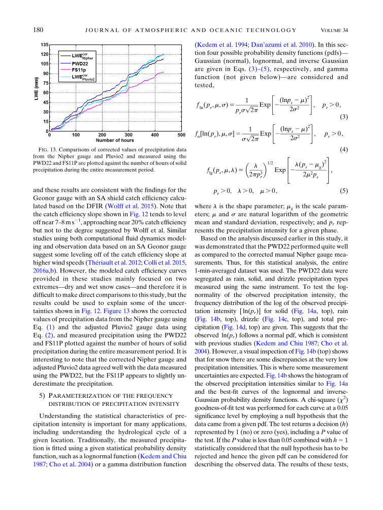
and these results are consistent with the findings for the

Geonor gauge with an SA shield catch efficiency calcu-

lated based on the DFIR (Wolff et al. 2015). Note that

the catch efficiency slope shown in Fig. 12 tends to level

off near 7–8ms21, approaching near 20%catch efficiency

but not to the degree suggested by Wolff et al. Similar

studies using both computational fluid dynamics model-

ing and observation data based on an SA Geonor gauge

suggest some leveling off of the catch efficiency slope at

higher wind speeds (Thériault et al. 2012; Colli et al. 2015,2016a,b). However, the modeled catch efficiency curves

provided in these studies mainly focused on two

extremes—dry and wet snow cases—and therefore it is

difficult tomake direct comparisons to this study, but the

results could be used to explain some of the uncer-

tainties shown in Fig. 12. Figure 13 shows the corrected

values of precipitation data from the Nipher gauge using

Eq. (1) and the adjusted Pluvio2 gauge data using

Eq. (2), and measured precipitation using the PWD22

and FS11P plotted against the number of hours of solid

precipitation during the entire measurement period. It is

interesting to note that the corrected Nipher gauge and

adjusted Pluvio2 data agreedwell with the datameasured

using the PWD22, but the FS11P appears to slightly un-

derestimate the precipitation.

5) PARAMETERIZATION OF THE FREQUENCY

DISTRIBUTION OF PRECIPITATION INTENSITY

Understanding the statistical characteristics of pre-

cipitation intensity is important for many applications,

including understanding the hydrological cycle of a

given location. Traditionally, the measured precipita-

tion is fitted using a given statistical probability density

function, such as a lognormal function (Kedem and Chiu

1987; Cho et al. 2004) or a gamma distribution function

(Kedem et al. 1994; Dan’azumi et al. 2010). In this sec-

tion four possible probability density functions (pdfs)—

Gaussian (normal), lognormal, and inverse Gaussian

are given in Eqs. (3)–(5), respectively, and gamma

function (not given below)—are considered and

tested,

fln(p

r,m,s)5

1

prs

ffiffiffiffiffiffi2p

p Exp

"2(lnp

r2m)2

2s2

#, p

r. 0,

(3)

fn[ln(p

r),m,s]5

1

sffiffiffiffiffiffi2p

p Exp

"2(lnp

r2m)2

2s2

#, p

r. 0,

(4)

flg(p

r,m,l)5

�l

2pp3r

�1/2

Exp

2642l(p

r2m

g)2

2m2pr

375,

pr. 0, l. 0, m. 0, (5)

where l is the shape parameter; mg is the scale param-

eters; m and s are natural logarithm of the geometric

mean and standard deviation, respectively; and pr rep-

resents the precipitation intensity for a given phase.

Based on the analysis discussed earlier in this study, it

was demonstrated that the PWD22 performed quite well

as compared to the corrected manual Nipher gauge mea-

surements. Thus, for this statistical analysis, the entire

1-min-averaged dataset was used. The PWD22 data were

segregated as rain, solid, and drizzle precipitation types

measured using the same instrument. To test the log-

normality of the observed precipitation intensity, the

frequency distribution of the log of the observed precipi-

tation intensity [ ln(pr)] for solid (Fig. 14a, top), rain

(Fig. 14b, top), drizzle (Fig. 14c, top), and total pre-

cipitation (Fig. 14d, top) are given. This suggests that the

observed ln(pr) follows a normal pdf, which is consistent

with previous studies (Kedem and Chiu 1987; Cho et al.

2004). However, a visual inspection of Fig. 14b (top) shows

that for snow there are some discrepancies at the very low

precipitation intensities. This is where some measurement

uncertainties are expected. Fig. 14b shows the histogramof

the observed precipitation intensities similar to Fig. 14a

and the best-fit curves of the lognormal and inverse-

Gaussian probability density functions. A chi-square (x2)

goodness-of-fit test was performed for each curve at a 0.05

significance level by employing a null hypothesis that the

data came from a given pdf. The test returns a decision (h)

represented by 1 (no) or zero (yes), including a P value of

the test. If theP value is less than 0.05 combined with h5 1

statistically considered that the null hypothesis has to be

rejected and hence the given pdf can be considered for

describing the observed data. The results of these tests,

FIG. 13. Comparisons of corrected values of precipitation data

from the Nipher gauge and Pluvio2 and measured using the

PWD22 and FS11P are plotted against the number of hours of solid

precipitation during the entire measurement period.


FIG. 14. (top) The frequency distribution of the natural log of the observed precipitation rate values for (a) rain,

(b) snow or solid, (c) drizzle, and (d) total precipitation. The black line represents the best-fit curve for a normal

distribution. (bottom) As in (top), but for the frequency distribution of precipitation rate values. The LogN and

InvG are the best-fit curves for lognormal and inverse Gaussian, respectively.


and the associated statistical parameters and values of

the coefficients, including arithmetic mean and variance

(V) of the distributions, are given in Table 4. As given in

the table, the null hypothesis was rejected for every pdf

considered and the calculated P values are much lower

than 0.05 except for the lognormal drizzle distribution.

This indicates that the considered distributions fit the

observed data. The gamma distribution function was

also tested, but the x2 null hypothesis statistical tests

indicated that the function is not suited for fitting the

solid phase precipitation (not shown in the table).

Generally, the rain distribution has higher mean and

variance values for all considered distributions, sug-

gesting more extreme events as compared to snow,

drizzle, and the combined case.

4. Snow density

As mentioned earlier, snow depth (Ds) was measured

four times daily using a snow ruler by taking the average

of 10 consecutive measurements. The snow density can

be calculated using Ds and the corrected Nipher gauge

measurements, assuming that LWEcorNipher as the snow

water equivalent (SWE). Following Rasmussen et al.

(2012), SWE is defined as the liquid equivalent of the

snow accumulation on the ground and snow depth (cm)

is a measurement of the total depth of the accumulation.

The liquid water equivalent (LWE) rate is the mass accu-

mulation rate of solid precipitation normally measured

using precipitation gauges (mmh21). Using these two

measurements, the snow-to-liquid ratio can be calcu-

lated as

ry5

10Ds

SWE, (6)

where Ds is given in centimeters and SWE is given in

millimeters. The snow density rs (g cm23) can be

given as

rs5

rw

ry

, (7)

where rw is the density of water, which is assumed to be

1 g cm23. Using the entire 6-hourly dataset mentioned

earlier, rs and ry were calculated. In this data analysis,

all the mixed-phase cases were eliminated from the data

to avoid the 10:1 snow density assumption mentioned

earlier. Figure 15 shows LWEcorNipher plotted against Ds

(Fig. 15a), and rs and ry plotted against the mean tem-

perature (Figs. 15b,c, respectively). The snow depth

varied from 0.2 to 8.4 cm, and the snow water equivalent

values varied from 0.2 to 9.93mm. As indicated in

Fig. 15a, LWEcorNipher is increasing with increasing Ds

following the best-fit nonlinear equation, defined as

LWEcorNipher 5 0:034D2

s 1 0:9Ds, r2 5 0:91, (8)

suggesting that the snow density is increasing with snow

depth. This is consistent with the findings using a much

more complex modeling approach (Sturn et al. 2010)

and large dataset analysis (Jonas et al. 2009). The snow

density ry varied from 4.2 to 35 with amean value of 12.2

or 0.082 g cm23. The mean value calculated in this study

is higher than the 10:1 ratio usually assumed for con-

verting Ds to snow water equivalent in Canada (Potter

1965; see Roebber et al. 2003 for discussions). Using 30

years of NWS Cooperative Summary of the Day data,

Baxter et al. (2005) found that themean of ry for most of

the contiguous United State to be close 13, which is very

close to the value found in this study.Onaverage, based on

the temperature-binned data as indicated by black circles,

ry is increasing with increasing temperature (Fig. 15c),

written as

ry5 0:0053T2

mean 2 0:275Tmean

1 9:92, r2 5 0:7 (9)

and hence the 10:1 ratio on average appears to be more

appropriate for warmer temperatures (T . 258C). A

TABLE 4. The best-fit coefficients for normal, lognormal, and inverse-Gaussian pdfs.

Distribution name pr phase m or mg s or l Mean V h P value

Lognormal—f ln(pr , m, s) Rain 20.829 1.551 1.453 21.26 1 2.2 3 1024

Snow 21.914 1.308 0.347 0.54 1 1.8 3 10227

Drizzle 21.633 0.859 0.282 0.09 1 0.124

Total 21.591 1.455 0.587 2.52 1 1.4 3 10225

Normal—fn[ln(pr), m, s] Rain 20.829 1.551 0.437 22.23 1 2.3 3 10248

Snow 21.914 1.308 0.148 13.68 1 0

Drizzle 21.633 0.859 0.195 5.57 1 1.4 3 10215

Total 21.591 1.455 0.204 18.36 1 1.5 3 102112

Inverse Gaussian—flg(pr , mg, l) Rain 1.311 0.166 1.311 13.57 1 1.0 3 1028

Snow 0.330 0.091 0.330 0.395 1 3 3 10236

Drizzle 0.276 0.248 0.276 0.055 1 0.01

Total 0.639 0.099 0.639 2.636 1 8.0 3 10281


recent study conducted by Boudala et al. (2014b) in a

relatively wetter and warmer climate in Vancouver,

British Columbia, Canada, showed that the mean value

of ry for wet snow was close to 10:1, which is on average

lower than the mean ry value determined in this study

but closer to the value determined for warmer temper-

atures as would be expected.

5. Summary and conclusions

In this paper precipitation amount and type, and snow

depth data collected during the 4Wing Cold Lake Re-

search Project covering the period from September 2014

to August 2015 using various instruments, including the

Vaisala PWD22 and FS11P sensors, the OTT Pluvio2

gauge, the Canadian Nipher and Type Bmanual gauges,

and a snow rule measuring depth, have been analyzed.

The analysis indicated that most (80% of the total) of

the measured snow intensities, by LWE, were relatively

low (,1.5mmh21; Fig. 9). During snow events the ob-

served temperature varied from 2358 to 48C and the

wind speed reached 12ms21 with amean value of 4ms21

and a standard deviation of 2ms21. Based on the 1-min-

averaged data collected using the optical PWD22 and

FS11P sensors, the precipitation events during the entire

measurement period represented only 12% of the total

time. Most of the reported precipitation types were snow

with a frequency of 8% followed by rain at 3% of the

time. There were only a few cases of drizzle and ice pellet

events. The precipitation types reported by the present

weather sensors were also compared with the hourly

human observation data for various temperature in-

tervals. When all the temperatures were included, the

observer reported no precipitation with a frequency of

86%,which was very close to the frequency of;88% that

was reported by both the PWD22 and FS11P. The human

observer reported snow and rain 10%and 4%of the time,

respectively, as compared to approximately 8% and 4%

measured by both PWD22 andFS11P sensors. This shows

that the observer reported only ;1% more snow cases,

indicating excellent agreement with the sensors. Ac-

cording to the observer, drizzle cases occurred 0.15% of

the time during the observation period, which was very

close to the value from the sensors (;0.4%). Both the

PWD22 andFS11P probes reported significantlymore ice

pellets events with frequencies of 0.14% and 0.2%, re-

spectively, as compared to the value reported by the

human observer, which was 0.024% of the time.

The amounts of 6-hourly precipitation measured us-

ing the Pluvio2 gauge with a single Alter shield, Cana-

dianNipher and Type B gauges, and theVaisala PWD22

and FS11P sensors were also compared. The comparisons

revealed that the collection efficiencies of the Pluvio2

gauge as compared to the manual measurements were

0.98 and 0.83 for liquid and mixed-phase cases, re-

spectively, indicating relatively good agreement with the

manual observations. For the solid phase, however, the

Pluvio2 gauge significantly undercaught with a ratio of

only 0.57, possibly due to wind effects. The Vaisala

PWD22 overestimated the amount as compared to the

manual measurements by 33% and 21% during solid

and liquid precipitation events, respectively. The FS11P

probe agreed with the manual measurements during

snow, but it overestimated the amount by about 30%

during rain. After correcting for the effect of wind dur-

ing snow for both the Canadian Nipher and the Pluvio2

FIG. 15. (a) Liquid wqater equivalent LWEcorNipher plotted againstDs, and (b) ry and (c) rs plotted against the mean temperature. The open

circles in (b) and (c) represents the temperature-binned data.


gauge, the data agreed remarkably well with the PWD22

measurements, but the FS11P measurement was still

slightly lower. Thus, these findings have demonstrated

the usefulness of emerging technologies, such as the

PWD22 and FS11P probes, showing that they can be

used for measuring snowfall in cold climates, where the

snowfall intensity tends to be relatively low.

After demonstrating the good performance of the

PWD22, the 1-min-averaged precipitation intensity fre-

quency distributions were obtained using this probe, in-

cluding the solid and liquid phases. Several probability

density functions, including gamma, normal, lognormal,

and inverse Gaussian, were used to fit the observed fre-

quency distributions. The goodness of the fits were tested

using null hypothesis chi-square statistics, and based on

these tests it was found that the observed precipitation

intensities can be described by lognormal and inverse-

Gaussian distributions.

Using the snow depth and corrected Nipher gauge

data, snow densities were derived. The snow density or

snow-to-liquid ratio varied from 4.2 to 35 with a mean

value of 12.2 or 0.082 g cm23, which suggests that the

mean value derived in this study is higher than the

10:1 ratio usually assumed for converting snow depth

to snow water equivalent in Canada. On average, the

snow density depends on temperature, increasing

with increasing temperature, and the 10:1 ratio ap-

pears to be more appropriate for relatively warmer

temperatures.

Acknowledgments. This work was partially funded by

the Department of National Defence (DND) and the

Canadian National Search and Rescue New Initiative

Fund (SAR-NIF) under the SAR Project (SN201532).

We like to thank Mike Harwood and Robert Reed for

helping with the installation of the instruments at Cold

Lake. The authors also would like to extend their thanks

to Ramond Dooley, Amy Slade-Campbell, and Gordon

Lee of DND for providing the hourly precipitation data,

and also Randy Blackwell for helping during the in-

strument installation process.

REFERENCES

Baxter, M. A., C. E. Graves, and J. T. Moore, 2005: A climatology

of snow-to-liquid ratio for the contiguous United States.Wea.

Forecasting, 20, 729–744, doi:10.1175/WAF856.1.

Boudala, F. S., G. A. Isaac, R. Rasmussen, S. G. Cober, andB. Scott,

2014a: Comparisons of snowfall measurements in complex

terrain made during the 2010 Winter Olympics in Vancouver.

Pure Appl. Geophys., 171, 113, doi:10.1007/s00024-012-0610-5.

——, R. Rasmussen, G. A. Isaac, and B. Scott, 2014b: Performance

of hot plate for measuring solid precipitation in complex terrain

during the 2010 Vancouver Winter Olympics. J. Atmos. Oce-

anic Technol., 31, 437–446, doi:10.1175/JTECH-D-12-00247.1.

Brandes, E. A., K. Ikeda, G. Zhang, M. Schönhuber, and R. M.

Rasmussen, 2007: A statistical and physical description of hy-

drometeor distributions in Colorado snowstorms using a video

disdrometer. J. Appl.Meteor. Climatol., 46, 634–650, doi:10.1175/

JAM2489.1.

Cho, H.-K., K. P. Bowan, and G. R. North, 2004: A comparison

of gamma and lognormal distributions for characterizing

satellite rain rates from the Tropical Rainfall Measuring

Mission. J. Appl. Meteor., 43, 1586–1597, doi:10.1175/

JAM2165.1.

Colli, M., R. Rasmussen, J. M. Thériault, L. Lanza, C. Baker, andJ. Kochendorfer, 2015: An improved trajectory model to eval-

uate the collection performance of snow gauges. J. Appl. Me-

teor. Climatol., 54, 1826–1836, doi:10.1175/JAMC-D-15-0035.1.

——, L. Lanza, R. Rasmussen, and J. M. Thériault, 2016a: Thecollection efficiency of shielded and unshielded precipitation

gauges. Part I: CFD airflow modeling. J. Hydrometeor., 17,

231–243, doi:10.1175/JHM-D-15-0010.1.

——, ——, ——, and ——, 2016b: The collection efficiency of

shielded and unshielded precipitation gauges. Part II: Mod-

eling particle trajectories. J. Hydrometeor., 17, 245–254,

doi:10.1175/JHM-D-15-0011.1.

Dan’azumi, S., S. Shamsudin, and A. Aris, 2010: Modeling the

distribution of rainfall intensity using hourly data. Amer.

J. Environ. Sci., 6, 238–243, doi:10.3844/ajessp.2010.238.243.

Goodison, B. E., P. Y. T. Louie, and D. Yang, 1998: WMO Solid

Precipitation Measurement Intercomparison. Final Rep.,

World Meteorological Organization Instruments and Ob-

serving Methods Rep. 67, WMO/TD-872, 211 pp.

Jonas, J., C. Marty, and J. Magnusson, 2009: Estimating the snow

water equivalent from snow depth measurements in the Swiss

Alps. J. Hydrol., 378, 161–167, doi:10.1016/j.jhydrol.2009.09.021.

Kedem,B., andL. S.Chiu, 1987:On the lognormality of rain rate.Proc.

Natl. Acad. Sci. USA, 84, 901–905, doi:10.1073/pnas.84.4.901.

——, H. Pavlopoulos, X. Guan, and D. A. Short, 1994: Probability

distributionmodel for rain rate. J. Appl.Meteor., 33, 1486–1493,

doi:10.1175/1520-0450(1994)033,1486:APDMFR.2.0.CO;2.

Mekis, É., and L. A. Vincent, 2011: An overview of the second

generation adjusted daily precipitation dataset for trend

analysis in Canada. Atmos.–Ocean, 49, 163–177, doi:10.1080/

07055900.2011.583910.

Metcalfe, J. R., and B. E. Goodison, 1993: Correction of Canadian

winter precipitation data. Preprints, Eighth Symp. on Meteo-

rological Observations and Instrumentation, Anaheim, CA,

Amer. Meteor. Soc., 338–343.

Potter, J. G., 1965:Water content of freshly fallen snow. CIR-4232,

TEC-569, Meteorology Branch, Dept. of Transport, Toronto,

ON, Canada, 12 pp. [Available from National Snow and Ice

Data Center User Services, University of Colorado, Campus

Box 449, Boulder, CO 80309-0449.]

Rasmussen, R.M., J. Hallett, R. Purcell, S. D. Landolt, and J. Cole,

2011: The hotplate precipitation gauge. J. Atmos. Oceanic

Technol., 28, 148–164, doi:10.1175/2010JTECHA1375.1.

——, and Coauthors, 2012: How well are we measuring snow: The

NOAA/FAA/NCARwinter precipitation test bed.Bull. Amer.

Meteor. Soc., 93, 811–829, doi:10.1175/BAMS-D-11-00052.1.

Roebber, P. J., S. Bruening, D. M. Schultz, and J. V. Cortinas Jr.,

2003: Improving snowfall forecasting by diagnosing snow

density. Wea. Forecasting, 18, 264–287, doi:10.1175/

1520-0434(2003)018,0264:ISFBDS.2.0.CO;2.

Sevruk, B., and S. Klemm, 1989: Catalogue of national standard

precipitation gauges. Tech. Rep. WMO, Instruments and

ObservingMethods, Rep. 39,WMO,Geneva, Switzerland, 50 pp.


http://dx.doi.org/10.1175/WAF856.1

http://dx.doi.org/10.1007/s00024-012-0610-5

http://dx.doi.org/10.1175/JTECH-D-12-00247.1

http://dx.doi.org/10.1175/JAM2489.1




http://dx.doi.org/10.1175/JAMC-D-15-0035.1

http://dx.doi.org/10.1175/JHM-D-15-0010.1

http://dx.doi.org/10.1175/JHM-D-15-0011.1

http://dx.doi.org/10.3844/ajessp.2010.238.243

http://dx.doi.org/10.1016/j.jhydrol.2009.09.021

http://dx.doi.org/10.1073/pnas.84.4.901

http://dx.doi.org/10.1175/1520-0450(1994)033<1486:APDMFR>2.0.CO;2

http://dx.doi.org/10.1080/07055900.2011.583910

http://dx.doi.org/10.1080/07055900.2011.583910

http://dx.doi.org/10.1175/2010JTECHA1375.1

http://dx.doi.org/10.1175/BAMS-D-11-00052.1

http://dx.doi.org/10.1175/1520-0434(2003)018<0264:ISFBDS>2.0.CO;2

http://dx.doi.org/10.1175/1520-0434(2003)018<0264:ISFBDS>2.0.CO;2

[Available online at https://www.wmo.int/pages/prog/www/

IMOP/publications/IOM-39.pdf.]

Sturn, M., B. Taras, G. E. Liston, C. Derksen, T. Jonas, and J. Lea,

2010: Estimating snow water equivalent using snow depth

data and climate classes. J. Hydrometeor., 11, 1380–1394,

doi:10.1175/2010JHM1202.1.

Thériault, J., R. Rasmussen, K. Ikeda, and S. Landolt, 2012: De-

pendence of snow gauge collection efficiency on snowflake

characteristics. J. Appl. Meteor. Climatol., 51, 745–762, doi:10.1175/

JAMC-D-11-0116.1.

——, ——, E. Petro, J.-Y. Trépannier, M. Colli, and L. G. Lanza,

2015: Impact of wind direction, wind speed, and particle

characteristics on the collection efficiency of the Double

Fence Intercomparison Reference. J. Appl. Meteor. Climatol.,

54, 1918–1930, doi:10.1175/JAMC-D-15-0034.1.

Wolff, M., K. Isaksen, A. Petersen-Øverleir, K. Ødemark,

T. Reitan, and R. Bækkan, 2015: Derivation of a new contin-

uous adjustment function for correcting wind-induced loss of

solid precipitation: Results of a Norwegian field study.Hydrol.

Earth Syst. Sci., 19, 951–967, doi:10.5194/hess-19-951-2015.

Yang, D., 2014: Double Fence Intercomparison Reference (DFIR)

vs. Bush Gauge for ‘‘true’’ snowfall measurement. J. Hydrol.,

509, 94–100, doi:10.1016/j.jhydrol.2013.08.052.——, S. Ishida, B. E. Goodison, and T. Gunther, 1999: Bias cor-

rection of daily precipitation measurements for Greenland.

J. Geophys. Res., 104, 6171–6181, doi:10.1029/1998JD200110.

——, D. Kane, Z. Zhang, D. Legates, and B. Goodison, 2005: Bias

corrections of long-term (1973–2004) daily precipitation data

over the northern regions. Geophys. Res. Lett., 32, L19501,

doi:10.1029/2005GL024057.


https://www.wmo.int/pages/prog/www/IMOP/publications/IOM-39.pdf

https://www.wmo.int/pages/prog/www/IMOP/publications/IOM-39.pdf

http://dx.doi.org/10.1175/2010JHM1202.1




http://dx.doi.org/10.5194/hess-19-951-2015

http://dx.doi.org/10.1016/j.jhydrol.2013.08.052

http://dx.doi.org/10.1029/1998JD200110

http://dx.doi.org/10.1029/2005GL024057

performance of emerging technologies for measuring solid

Documents