performance monitoring in communication networks

PERFORMANCE MONITORING IN COMMUNICATION NETWORKS

Doctoral thesis

Thomas Lindh

Laboratory for Communication Networks IMIT, Department of Microelectronics and Information Technology

KTH, Royal Institute of Technology

Stockholm 2004

Performance Monitoring in Communication Networks A dissertation submitted to the Royal Institute of Technology (KTH) for the degree of Doctor of Philosophy © 2004 Thomas Lindh Royal Institute of Technology (KTH) Department of Microelectronics and Information Technology Laboratory for Communication Networks Electrum 229, SE-16440 Sweden TRITA-IMIT-LCN AVH 04:02 ISSN 1651-4106 ISRN KTH/IMIT/LCN/AVH-04/02--SE Printed in 150 copies by Universitetsservice US AB, Stockholm 2004

1

ABSTRACT Performance monitoring in communication networks, which is the main topic

of this thesis, is an essential part of performance and network management. The applications cover a number of different areas such as daily operations and main-tenance, usage information for billing purposes, customer reports, traffic control, planning, and dimensioning.

The main purpose of the thesis is to develop a single method for measurement of the most significant network performance parameters in IP networks. It is a continuation from a previous licentiate thesis that focused on performance moni-toring in cell-based networks.

The development of a measurement method that combines active and passive approaches using monitoring blocks is the main contribution of this work. A traffic flow performance meter based on these principles has been implemented as an extension to the open source flow meter NeTraMet and tested. The resolu-tion and precision of the results are determined by the size of the monitoring block, which is the method’s main parameter. Relevant statistical issues regard-ing packet losses and delays are analysed. Finally, the measurement method is discussed in the context of applications, as well as network and service manage-ment systems in general.

3

PREFACE The topic of this doctoral thesis is performance management, especially meas-

urement and monitoring aspects. It is a continuation and extension of a previous licentiate thesis that covered performance monitoring in cell-based networks. The thesis focuses on methods and models for performance monitoring in IP networks.

The licentiate thesis was completed at the Department of Industrial Control Systems, Royal Institute of Technology (KTH). Thereafter my affiliation has been the Department of Microelectronics and Information Technology in the Laboratory for Communication Networks at KTH, where Professor Gunnar Karlsson has been my supervisor. Telia Engineering (later Telia Prosoft, Ki Con-sulting, and today a part of TietoEnator) and KTH Syd have supported the re-search project financially and in many other ways. The cooperation with Nevil Brownlee (University of Auckland, New Zealand, and CAIDA, San Diego, US) has been important for the progress of the work. A number of students at KTH Syd in Haninge have also made valuable contributions to the implementation and testing of the measurement method. The thesis is mainly based on the papers described in the section List of Publications.

February 2004 Thomas Lindh

5

ACKNOWLEDGEMENTS First, I like to thank Professor Gunnar Karlsson at the Laboratory for Commu-

nication Networks (LCN) at KTH/IMIT who has been my supervisor during the doctoral studies. Without the support and constructive ideas from Gunnar, this dissertation work would not have been possible. I also like to thank Johan Schu-bert who was my supervisor during the licentiate studies at Industrial Control Systems (KTH/IMIT). The discussions with Johan were of invaluable help dur-ing the work with the licentiate thesis.

The implementation of the measurement method in NeTraMet (developed by Nevil Brownlee at the University of Auckland, New Zealand, and CAIDA, San Diego, US) was an important step forward. Many thanks Nevil for your help and cooperation, especially for writing the code that implements the method based on monitoring packets in NeTraMet.

I want to thank Professor Gerald Maguire and Professor Rolf Stadler at LCN for their constructive comments.

I am grateful to Ibrahim Orhan at KTH Syd for his interest and valuable sup-port with the laboratory tests. A number of student thesis projects at KTH have contributed to the work. I specially like to mention Per Nordén, Daniel Lind-qvist, Leif Larsson, Björn Olander, Ola Söderholm, Shelton Videau, Helene Jonsson, Yeliz Erdogan, and Erik Olsson.

I also thank Professor Jorma Jormakka at the Helsinki University of Technol-ogy for sharing his experiences from the European project QUASIMODO, and Henk Uijterwaal and Mark Santcroos at RIPE for providing traffic data.

The research studies have been carried out in parallel with my teaching at the College of Applied Engineering in Haninge. I like to thank the former head of KTH in Haninge Lars Källander whose efforts made this project possible. Inge Jovik, head of KTH Syd today, has continued this support.

The operator Telia has sponsored the main part of my studies and research pro-jects. I am grateful to Östen Mäkitaalo at Telia Research who started this coop-eration. Several divisions at Telia and many helpful persons have supported my work. I specially would like to mention Birger Wörkvist, Harry Vourela, Arne Lindgren and Patrick Wilkinson at former Telia Prosoft, Alexander Latour-Henner at Telia, Nils Björkman at Telia Research, and Johan Eriksson, Anders Martin and Mats Rihed at Skanova (today TeliaSonera).

7

TABLE OF CONTENTS ABSTRACT ............................................................................................................ 1 PREFACE ............................................................................................................... 3 ACKNOWLEDGEMENTS.......................................................................................... 5 PURPOSE AND CONTRIBUTION ............................................................................ 11 OUTLINE OF THE THESIS ..................................................................................... 13 CHAPTER I: INTRODUCTION ................................................................................................... 15

1. Communication Networks....................................................................... 15 2. Management of Communication Networks............................................. 16 3. Performance Management of Communication Networks........................ 18

CHAPTER II: PERFORMANCE MONITORING IN DATAGRAM NETWORKS ................................... 21

1. Applications and Objectives.................................................................... 21 2. International Standardisation................................................................... 21 3. Monitoring of Service Level Agreements ............................................... 23 4. Prerequisites ............................................................................................ 23 5. Measurement Methods ............................................................................ 24 6. Monitoring at the Network Level ............................................................ 25 7. End-to-End Monitoring of Communication Services.............................. 28 8. Directly Related Work ............................................................................ 28

CHAPTER III: A TRAFFIC FLOW PERFORMANCE METER ........................................................... 31

1. Purpose and Design................................................................................. 31 2. An Embedded Monitoring System .......................................................... 33 3. A Stand-Alone Traffic Flow Performance Meter .................................... 56 4. Applications ............................................................................................ 64 5. System Aspects of the Method ................................................................ 66 6. Statistical Aspects of the Method ............................................................ 69 7. Evaluation of the Method ........................................................................ 80

CHAPTER IV: PERFORMANCE MONITORING IN VIRTUAL CIRCUIT NETWORKS.......................... 83 CHAPTER V: SUMMARY AND FUTURE WORK .......................................................................... 87 LIST OF PUBLICATIONS ....................................................................................... 91 REFERENCES ....................................................................................................... 93 APPENDIX A:......................................................................................................101 Results from Laboratory Tests of a Performance Flow Meter Using NeTraMet APPENDIX B:......................................................................................................115 Statistical Properties of Measurement and Simulation Data Used in the Thesis

8

APPENDIX C.......................................................................................................123 Examples of Descriptive Statistics for Packet Losses APPENDIX D:......................................................................................................133 Results from Simulations of Markov Models of Loss Periods and Loss-Free Periods Appendix E: ......................................................................................................139 Comparison of Measurement Results for Periodic and Random Sampling APPENDIX F: ......................................................................................................143 Sampling Methods - Test Results and Uncertainty Estimates APPENDIX G:......................................................................................................149 Performance Management in Switched ATM Networks, IS&N 1998 (Fifth International Conference on Intelligence in Services and Networks), Antwerpen, May 1998. APPENDIX H:......................................................................................................161 Methods and Models for In-Service Monitoring and Estimation of Cell Losses in ATM Networks, ICT 1998 (International Conference on Telecommunications), Porto Carras, Greece, June 1998.

11

PURPOSE AND CONTRIBUTION The main purpose of the thesis is to develop a single method for measurement

of the most significant network performance parameters in IP networks. It is a continuation from a previous licentiate thesis that focused on performance moni-toring in cell-based networks.

The approach is to use: ♦ an in-service technique that is meant to reflect the behaviour of ac-

tual user traffic and not merely test traffic, ♦ a direct method that does not rely on the accuracy of certain traffic

models, and ♦ a suitable combination of active and passive measurement tech-

niques.

The measurement method has the following goals. ♦ To use a single procedure to measure and estimate the main per-

formance parameters in IP networks: packet losses, packet delays, packet delay variations, and throughput.

♦ To obtain measures, and estimates, of these parameters with high resolution and not merely long-term averages for the entire meas-urement period.

The method is designed as a combination of traffic flow meters and dedicated monitoring packets to obtain these goals. It introduces a parameter and a specifi-cation that determine the accuracy and resolution of the results. The size of a monitoring block determines the precision and resolution of the delay estimates, and the resolution of the loss and throughput metrics. The block size can be ex-pressed in terms of time-periods or number of packets or bytes. The packet filter specification controls the granularity of the traffic flows that are being moni-tored. The performance data produced by the method can provide operators and customers with continuous performance reports, and can also support traffic and network control functions such as connection admission control and traffic engi-neering.

The main contribution is the development of a method based on monitoring blocks. A traffic flow performance meter has been implemented as a part of the open source flow meter NeTraMet and tested. The results are analysed with respect to the size of the monitoring block, which is the main parameter. Rele-vant statistical issues regarding packet losses and delays have been analysed. Finally, the measurement method is also discussed in the context of applications, and network and service management systems in general.

13

OUTLINE OF THE THESIS The thesis is organised as follows. Chapter I consists of a general background

that places performance measurements in a broader context. Some aspects of telecommunications management, especially performance monitoring, are sum-marised. Chapter I closes the loop back to the initial work on network manage-ment, published in the licentiate thesis.

Chapter II is a survey of related work in performance measurement in IP net-works. It can be read as a state of the art survey of this field.

Chapter III contains the main contribution of the thesis. A framework for a measurement method based on monitoring blocks that combines active and pas-sive approaches is outlined. Simulations based on traffic data and different im-plementations of the method are presented. The main result is a traffic flow per-formance meter implemented as a part of NeTraMet. Applications and monitor-ing system aspects of this method are also considered. Finally, statistical issues related to packet losses and packet delays are analysed. Appendices A to F are related to this chapter.

Chapter IV contains some aspects of performance monitoring in connection oriented packet networks, especially ATM networks. This work was a part of the licentiate thesis. Appendices G and H consist of two papers that summarise the main contributions in this area.

A summary, ideas for future work and a list of publications conclude the the-sis, in Chapter V.

15

CHAPTER I

INTRODUCTION

This introductory chapter gives a brief background to the results in perform-

ance measurement and monitoring presented in the following chapters of the thesis. Some of the general trends in network management are considered. Per-formance management is discussed in the context of a top-down approach that comprises the interaction between management and control functions in the network and service domains.

1. Communication Networks The need for measurement of performance parameters to support operations,

management, and planning of communication networks has increased in recent years. One reason is that the Internet protocol (IP) seems to becoming the domi-nant networking protocol for providing information services in fixed and mobile networks, either to replace or complement the traditional telecommunication services. Several new service architectures have been proposed in order to extend the traditional best-effort service. IP networks are no longer limited to transfer-ring pure data. Today the expectations rather seem to be that IP will be the com-mon carrier for multiservice communications. Besides the original goals of ro-bustness, simplicity and optimal network utilisation, IP networks are also meant to provide high-speed services with strict performance requirements.

The great variety of communication services has added complexity to the in-formation infrastructure. Databases and other distributed computer systems have become an integral part of today’s communication networks. Not merely net-work performance but also the end-to-end behaviour of communication services has become increasingly important for network operators and service providers.

These new conditions and objectives have raised a number of open issues and challenges for researchers, engineers, and operators. An important part of the solutions to the problems is to develop effective methods for performance meas-urement and monitoring to be used in operation and management of communica-tion networks.

16

2. Management of Communication Networks A consequence of the dominant role of TCP/IP is that the simple network

management protocol (SNMP) today has a major impact on how monitoring and control of networks and services are performed [1]. The simplicity of SNMP is the main reason for its success, but probably also its weakest point. A decade ago, the telecommunication operators and vendors favoured a more powerful, but also more complex model for network management. It was mainly based on the OSI recommendations for network and systems management. This architecture from ITU-T for telecommunications management network (TMN) has not been as successful and widely implemented as SNMP [2]. However, many of the shortcomings in Internet network management that still remain to be solved, such as information modelling, were addressed in the TMN framework. Some of the work today on more powerful information models, e.g. the common information model (CIM) can to some extent be seen as an attempt to modernise and further develop some of concepts and ideas in TMN [3].

The rapid development in data communications and networking during the last decade has led to major changes in network management. Some trends in this area are summarised below [4]. ♦ Service management focuses on the delivered communication ser-

vices and not merely on the network aspects. ♦ Distributed systems in telecommunication networks call for meth-

ods and models for management in a distributed environment. New software solutions such as mobile agents and new network para-digms such as active networking have been studied for manage-ment purposes.

♦ Web-based management using HTTP and more powerful informa-tion models (CIM) are promoted by e.g. the Distributed Manage-ment Task Force (DMTF) [3].

♦ Policy-based management has been an active research field often targeted at configuration management.

♦ Integration between network management and systems manage-ment has become a necessity since information systems are integral parts of today’s networks.

♦ Management solutions based on the business processes in order to structure, and possibly automate management functions, are vital for operators.

♦ Open and standardised interfaces between network elements and management systems and between different management systems are still important implementation issues.

Telecommunications management covers a wide area. To find a precise defini-tion that delimits its scope is not easy. Figure 1 illustrates how the concepts are used in this thesis. First, a separation is made between the network and service

17

domains, and secondly between management and control. This idea was further developed in [4].

The time scale for actions and responses in network management is often in the order of seconds, minutes, and even longer periods. Real-time control nor-mally works at shorter time-scales. Another difference is that management sys-tems interact with and are controlled by human operators. Real-time control systems typically interact (slowly) with management systems, e.g. for configura-tion and parameter tuning.

The borderline between management and control is not obvious, especially in modern telecommunication systems. Whether real-time control and management should be separated or integrated, and to what extent, has been debated for a long time. Contributions can be found in [5], [6], [7] and [8]. The interaction between the management plane and the control plane for performance management in switched ATM networks is discussed in Chapter IV and Appendix G. In general, the solution is to find an appropriate balance between integration and separation of management functions and control functions.

Servicemanagement

Serv i ce domain

Ne t work domain

Serv i ce co n trol

Networkmanagement

Network control

Figure 1: Relations between management and control in the network and service do-mains.

The relation between the network domain and the service domain has become increasingly important due to the fast introduction of new services and overlay service networks. Management from the service-level is typically concerned with end-to-end services and applications, service level agreements, customer con-tacts, and interfaces to customer-based management systems or other service providers. The management activities are carried out in close interaction with the service control functions (resource and connectivity management, session control and service signalling systems, etc.). It also encompasses the operation and main-tenance of resources in the service domain such as servers, and databases. More-over, the service management system is forced to interact with corresponding functions in the network domain. As in the previous case, the key issue is to achieve a proper balance between management and control functions. Contribu-tions to this field can be found in e.g. [9] and [10].

A final general observation is that the management architectures and the actual telecommunication processes often seem to evolve rather separately. A manage-ment system needs on the one hand to be robust against at least moderate

18

changes in the telecommunication process. On the other hand, it is decisive to adopt an integrated approach to the management functions and the managed network or service processes. One striking example is the ambitious and com-prehensive TMN model that failed to adapt to the rapid development and de-ployment of IP networks.

The top-down approach to management and control functions depicted in Fig-ure 1, introduced in [4], has been applied to performance management and moni-toring in this thesis.

3. Performance Management of Communication Networks

3.1. The Scope Performance management, which is one of the classical areas in network man-

agement, is composed of three major elements: monitoring, analysis, and con-trol. In general terms, the goal of performance management is to ensure that the network operates efficiently and to maintain the quality of service (QoS) in a cost-effective manner. These activities are based on a model consisting of a set of performance objectives. Since the interpretation of these concepts tends to vary a great deal, some of the definitions used by ITU-T are given below.

Quality of service (QoS) is defined as the “collective effect of service perform-ances which determine the degree of satisfaction of a user of the service” [113]. The quality-of-service parameters are focused on the user-perceivable effects and should be described in network independent terms understandable by both the user and the service provider. The definition of QoS parameters should be based on events and states observable at the service access-points.

Network performance has been defined as “the ability of a network or a net-work portion to provide functions related to communications between users” [113]. Network performance is measured in terms, which are meaningful to the network provider and are used for the purpose of system design, configuration, operation and maintenance, and defined independently of terminal performance and user actions [114]. QoS is essentially an end-to-end concept of performance between users while network performance parameters relate to conditions within or at the boundary of a network. Thus, the mapping between network parameters and quality of service is not a simple one-to-one relationship. The QoS parame-ters should be network independent and understandable by the customer. Ac-cording to [115] “an essential difference between QoS and network performance (NP) is that QoS is user oriented while NP is network provider (or technically) oriented”.

Grade of service (GoS) is a related term also defined by ITU as: “A number of traffic engineering variables used to provide a measure of adequacy of a group of resources under specified condition; these grade of service variables may be the probability of loss, dial tone delay etc.” [116]. Grade of service can be measured at service access points or within networks. Accordingly, GoS can be identical to

19

network performance or quality of service variables. However, GoS variables can also be characterised by parameters that are not measurable. Thus, there is no general correspondence between GoS and network performance [85].

According to recommendation M.3400 (within the TMN architecture) from ITU-T, performance monitoring involves continuous collection of data concern-ing the performance of network elements. This process is closely related to fault management (alarm surveillance). While acute fault conditions and failure events will be detected by alarm surveillance, performance monitoring is designed to indicate low rate and intermittent error conditions over a time interval. The pur-pose is to measure the overall quality in order to detect performance degradation. M.3400 and Q.822 from ITU-T contain generic functions (request for data, start and stop collection, and report), traffic status monitoring functions (service availability, status of control, congestion, etc.) and traffic performance monitor-ing functions (assessment of the current performance of the network and the traffic being carried).

Performance control involves generic functions (request, set and test perform-ance attributes and thresholds, etc.), traffic control functions (apply, modify, remove manual and automatic control), and traffic administrative functions (es-tablish, change, remove measurement schedule, etc.). This process is closely related to configuration management and traffic control functions.

3.2. New Challenges Performance management generally comprises monitoring, analysis, and con-

trol functions. The rapid and ongoing changes in telecommunications mentioned in the previous sections brought new challenges, especially to performance man-agement.

♦ Multiservice networks and introduction of new service architec-tures that provide different service classes often based on statistical guarantee requirements are emerging.

♦ Measurements and estimates are needed in order to monitor and verify service level agreements (or specifications) between opera-tors and customers, and to support traffic control functions, such as admission control and traffic engineering.

♦ The development of new services and service overlay platforms call for performance monitoring and control above the network level, often for end-to-end connections between clients and servers.

♦ Traffic flows (defined as a unique combination of source and desti-nation addresses on the network and transport levels, and transport protocols) is an essential entity for traffic control of end-to-end per-formance.

♦ There is a need for an integrated approach to measurement, moni-toring, and traffic control functions.

The remaining parts of this thesis focus on performance measurements and monitoring of packet networks.

21

CHAPTER II

PERFORMANCE MONITORING IN DATAGRAM NETWORKS

This chapter contains a survey of performance measurement methods for IP

networks and related work that has been useful for the thesis.

1. Applications and Objectives There are a number of reasons for operators of IP networks to measure and

verify the actual level of performance in their networks. Besides traditional areas such as daily operations, usage information for billing purposes, customer re-ports, planning, and dimensioning, the ambitions of operators to offer services with different quality assurances to customers underline this need even more. This thesis is based on the conviction that measurement and monitoring func-tions have to be determined by an operator’s policy and objectives for perform-ance management and adjusted to the type of services that are offered

2. International Standardisation Since measurement in IP networks is a relatively new and growing area there

is a need for international standards. The most important contributors to this process are the IP performance metric (IPPM) working group in the Internet Engineering Task Force (IETF) and ITU-T working group on performance of networks and services (T1A1.3). IPPM has issued the following requests for comments (RFCs).

♦ Framework for IP performance metrics (RFC 2330). ♦ IPPM Metrics for measuring connectivity (RFC 2678). ♦ A one-way delay metric for IP performance metrics (RFC 2679). ♦ A one-way packet loss metric for IP performance metrics (RFC

2680). ♦ A round-trip delay metric for IP performance metrics (RFC 2681).

22

♦ A framework for defining empirical bulk transfer capacity metrics (RFC 3148).

♦ One-way loss pattern sample metrics (RFC 3357). ♦ IP packet delay variation metric for IP performance metrics (RFC

3393). ♦ Network performance measurement with periodic streams (RFC

3432).

ITU-T has published the recommendation “Internet protocol data communica-tion service - IP packet transfer and availability performance parameters” (Y.1540) [11]. Recommendation Y.1541, “Network performance objectives for IP-based services” [124], specifies performance values for the parameters in Y.1540.

In summary, ITU-T and IETF have specified the following categories of net-work performance parameters. ♦ IP packet loss ratio is defined as the number of lost packets divided

by the number of sent packets. This metric does not tell anything regarding the distribution of losses over the measurement period, such as the distance between lost packets. A possible measure would be the mean length of loss-free periods and loss periods re-spectively. Similar metrics have been used in bit error statistics, e.g. error-free seconds. Loss patterns are discussed in RFC 3357 [40].

♦ IP packet transfer delay is the one-way transfer delay between sender and receiver. Two-way delay (round trip time) does not re-quire clock synchronisation and is therefore easier to measure. Tra-ditionally an analysis is based on two-way delay with the assump-tion that the delay is symmetric.

♦ The packet delay variation is especially relevant for real-time ser-vices. It is defined as the difference between one-way delays in pairs of packets in RFC 3393 [41]. ITU-T defines an end-to-end two-point IP packet delay variation (vk ) for a packet k, as the dif-ference between the packet delay (xk ), and a reference packet delay (d1,2), vk = xk – d1,2. The reference delay (d1,2) is the transfer delay experienced by the first packet sent between the measurement points. As an alternative, the average delay can be used.

♦ IP packet error ratio is the ratio of the number of errored packets to the total number of transmitted packets.

Besides these quality-of-service metrics, the utilised capacity often is a rele-vant parameter to measure. Recommendation Y.1541 mentions metrics for suc-cessfully transmitted packets and bytes as an issue for further study [124]. IETF has defined a bulk transport capacity as a measure of a network’s ability to trans-fer significant quantities of data with a single congestion-aware transport connec-tion (e.g., TCP) [125].

23

IETF has also adopted a number of related RFCs especially for traffic flow measurements. The RTFM (real-time traffic flow measurement) working group has issued these RFCs.

♦ RTFM: applicability statement (RFC 2721). ♦ Traffic flow measurement: architecture (RFC 2722). ♦ Traffic flow measurement: meter MIB (RFC 2723). ♦ SRL: a language for describing traffic flows and specifying actions

for flow groups (RFC 2723). ♦ RTFM: new attributes for traffic flow measurement (RFC 2724).

3. Monitoring of Service Level Agreements Performance measurements can be used to monitor service level agreements

between operators and users (customers). Two examples of specifications of service level guarantees are given below. ♦ A service category with guarantees for a low level of packet losses,

e.g. the packet loss ratio < x percentage and the loss-free periods > y seconds (or number of packets) on the average.

♦ A service category with guarantees for a low level of packet delays, e.g. a mean delay < z ms (with specified confidence level and in-terval), a maximum delay below u ms, and a mean delay variation less than v ms.

4. Prerequisites Performance measurement in connectionless networks such as IP is associated

with some special requirements. In connection-oriented networks, every packet or cell belongs to a logical connection with a predetermined path. However, in connectionless networking there is no guarantee that each datagram in a session follows the same path from sender to receiver and arrives in the original order. The source and destination network addresses in the IP header tell merely from which endpoint the packet originates and at which endpoint it will terminate. Given two measurement points, M1 and M2 at the edge of a network, it is not possible to find out solely based on the packet header information if a packet that arrives at M2 has passed through M1. Packet networks based on virtual circuits on the contrary use labels that uniquely identify the path set up for the actual con-nection. However, in some cases such as MPLS (multi-protocol label switching), labels can be shared by several connections (label merging). In these cases, addi-tional information is needed to determine the packet’s path prior to its arrival at M2. Another difference compared to for example cell-based networks is that IP allows variable packet sizes, which has to be accounted for in estimating trans-mission rates as well as the loss ratio.

24

5. Measurement Methods Methods for measuring network performance parameters are usually divided

into two categories: passive methods, such as sniffers and traffic meters, and active methods, where dedicated probe packets are generated. The idea behind passive methods is to capture packets in order to collect and store information from various fields within the packet header. Traditional sniffers, protocol ana-lysers and traffic meters are all based on this principle. Well-known tools such as Tcpdump [12], Ntop [13], NeTraMet [14], Netflow [15] and various RMON probes are based on a passive measurement technique.

Unlike active tools, passive monitors do not add extra traffic load to the net-work. Besides this non-intrusive character, passive methods enable gathering of large amount of detailed information. However, recording and logging of packet traces in high-speed networks often require special arrangements for collection, processing, and storage of large amount of data. Active methods are on the other hand based on injecting probe packets. Some examples of tools based on active methods are RIPE’s test traffic measurement project [43], the active measure-ment project (AMP) from NLANR [16], PingER from SLAC [17] and Surveyor [18]. The service assurance agent (SAA) from Cisco is one of many tools devel-oped by vendors [19].

SNMP is sometimes referred to as a special measurement method. However, it is also a way to organise and structure information (specifically management information) in network elements, and to retrieve information from those MIBs (management information bases). Performance information stored in databases that support the MIB structure is collected by means of either passive or active methods. Many commercial systems and freely available tools, e.g. MRTG (multi router traffic grapher), are configured to poll traffic counters and other performance information stored in a router’s MIB tree. Remote network monitor-ing (RMON), which can be seen as a step towards distributed monitoring, is also structured as a MIB [20]. A manager can obtain traffic information from RMON probes using SNMP.

Performance monitoring methods may also be classified as being either in-service or out-of-service. Out-of-service methods are only applied to test traffic, while the purpose of in-service methods is to monitor the actual user traffic. In-service monitoring may be performed using non-intrusive passive methods or by means of various active methods.

25

6. Monitoring at the Network Level Network performance parameters (packet losses, packet delays and packet er-

rors) can be measured using either an active or a passive technique. The main difference is that in an active approach probe packets are inserted for measure-ment purposes. The accuracy and granularity of the results therefore depend on the probing process. However, if the ratio of probe packets becomes relatively high the measurement result itself will be affected. Emstad and Viken [21] have studied this aspect. Active probing has several advantages. It is often simple to implement and the capacity requirements for are low compared to passive tools, which often need high-speed interfaces. An active approach is often more flexi-ble. Probe packets can be sent to any destination point at any time. A passive technique has to adapt to the current traffic conditions.

The accuracy of active measurements depends not only on the probing (or sampling) process, but also on how the network treats the probe packets. If the measurement packets do not experience the same conditions as the user data traffic, systematic error (bias) is difficult to avoid. If for example ICMP is used for the probe packets or the packet size differ significantly from the data packets it would likely cause systematic errors. Studies indicate that packet loss estimates are less precise than packet delay estimates using an active technique. Heegaard and Viken found that active measurements show poor precision in estimating the loss ratio during periods of congestion [22]. They propose an adaptive algorithm for active probing where the probing intensity is determined by the variance of the delays. The main idea is to send the test packets more frequently when the traffic load increases.

Several active tools for bandwidth measurement based on packet dispersion techniques have been presented. Most such methods rely on sending pairs or trains of probe packets with an inter-packet spacing that is small enough to cause queuing at the bandwidth bottleneck of a network path. The dispersion of long packet trains is inversely proportional to the available bandwidth according to [23]. Dovrolis has shown that this instead corresponds to what he calls the as-ymptotic dispersion rate [24]. The Pathload tool sends streams of K packets of length L at rate R. If R is higher than the available bandwidth A, the one-way delays of successive packets will increase [25]. An iterative algorithm where R is increased if R < A, and decreased if R > A is then applied to find the available bandwidth.

To measure one-way delays the internal clocks of the measurement points have to be synchronised with each other in order, using e.g. the network time protocol (NTP) [26]. Studies show that it often is difficult to achieve sufficient stability and precision in measurements that rely on NTP servers ([27] and [28]). Pásztor and Veitch found that a client synchronised to a NTP server via Ethernet can achieve accuracy around one millisecond and that NTP is strongly affected by changes in network delays. GPS (global positioning system) receivers directly connected to the measurement equipment is an alternative to improve the preci-sion considerably. To use clock pulses from cellular systems (e.g. CDMA) is

26

another possibility. One important error source in delay measurements is the stability and quality of the internal computer clock. A study by Pásztor and Veitch show that PCs with high-precision software clocks work well for round-trip time measurements, which in many cases are sufficient [27].

A passive approach requires direct access to the actual user traffic, and there-fore provides more traffic information than active methods. This means that measurement equipment and storage facilities have to keep up with the rapidly increasing packet rates. Every packet must be captured and matched against the filter specifications, possibly also associated with a timestamp; the header infor-mation must be read or stored in order to update counters, and so on. This proc-ess has to be repeated for each packet at line speed. Since the packet rates in today’s networks are high and increasing, a sampling procedure is often neces-sary.

Passive methods have mostly been used in one-point measurement to study throughput, packet sizes, the protocol distribution, arrival times, and round-trip times (e.g. using TCP header information). Should a passive technique be ap-plied for measuring delays, losses, and throughput between two points in the network, a number of difficulties has to be solved. As for active one-way delay measurements, synchronised clocks are needed, and a timestamp has to be stored for each captured packet at both points. Packets that are selected by the first measurement point have to be detected by the second measurement point. Trajec-tory sampling [29] and IP traceback [30] address this problem, but for different application purposes. In both cases, a hashing function is applied to parts of the packet in order to produce a unique label that identifies the packet. Only the part of the packet that is invariant to changes is possible to use. The probability of label collision is determined by how many bits of the packet that the hash func-tion includes. Trajectory sampling aims at estimating the proportion of traffic flows that follow certain paths from an ingress node to an egress node. Perform-ance metrics such as the loss ratio can also be estimated. One sampling hash function is used for the selection of packets and another hash function for pro-ducing the label that identifies the sampled packet. The purpose of IP traceback is to trace intruders that have succeeded to pass a firewall back to the source. Zseby has studied different sampling algorithms for one-way passive delay measurements using two synchronised systems [31].

Traffic flow information such as data rates, protocols, and packet length distri-butions are collected by means of passive methods. Traffic flow meters can be seen as a special case of such passive tools. A flow is defined as a unique combi-nation of source and destination network addresses at the network and transport level plus the transport protocol. The meter is configured to use packet header information to update traffic counters related to specific attributes for the defined flows. The aim of the IETF working group IPFix (IP flow information export) is to find a common standard to replace the different flow formats, e.g. NetFlow from Cisco and sFlow used by Foundry Networks [32]. The IETF working group PSAMP is a related activity that focuses on sampling aspects in passive meas-urement [33]. Due to the increasing link speed, sampling is often a necessity.

27

The methods and tools discussed previously in this section are direct and not based on a model. Duffield and others have developed a multicast-based infer-ence system of network-internal loss characteristics [34]. It is a maximum likeli-hood estimator based on a binomial stochastic model for packet losses on succes-sive independent links. The inference of losses on internal links in a network is based on losses of multicast probing traffic observed by multicast receivers. The work has been extended to network-internal delay distributions [35].

Lewis and others have presented a measurement-based approach to estimate the bandwidth requirements (referred to as essential bandwidth technology) for given levels of quality-of-service. The method uses an entropy (or rate) function that is estimated from measurements of packet arrival data. The method uses a result from the theory of large deviations, where the loss probability, as a func-tion of the buffer size, decays exponentially. The decay rate is determined by the capacity of the server (the queue length) and the arrival statistics. The core of the essential bandwidth technology is to measure and estimate the arrival entropy function. For given maximum loss probabilities and maximum delays, the corre-sponding available (essential) bandwidth can be determined [36].

The most common method used in large commercial performance monitoring systems (e.g. eHealth from Concord Communications [121], Inc and InfoVista Corp. [122]) is to retrieve management information from the network elements by means of SNMP. The RMON MIB is structured to support passive probes that collect traffic statistics. However, RMON 1 is limited to the link layer but RMON 2 comprises the higher layers including the application protocols. RMON probes are mainly tools for traffic and protocol analysis and are not pri-marily designed for performance measurement of packet losses, delays, and jitter.

Performance degradation in networks is often related to routing issues. A number of tools and systems have been developed to monitor routing paths, routing updates, and convergence times. However, this aspect is not within the scope of this thesis.

28

7. End-to-End Monitoring of Communication Services

Monitoring of traffic between the end-users, such as clients and servers, is of-ten necessary to get a complete picture of the perceived performance. It may also be a requirement for verification of service level specifications between custom-ers and operators. These measurements can be done at the network level, but are often preferably performed at the transport or application layers. This approach also makes it possible to determine how the total end-to-end losses and delays are distributed between the core network, access network and end-stations. Be-side packet losses and retransmissions, the server response time is an important performance parameter in client-server communication. These measurements have to be tailored for the specific service: such as requests from servers that handle domain names, emails, web pages, data files, or directories. A number of active tools act as clients that send probing requests to the actual server to meas-ure response times and other performance parameters. The certainty of the sam-pling results has to be analysed in terms of bias, confidence levels, and statistical errors.

A passive approach with a single measurement point can take advantage of feedback information provided by TCP (acknowledgments) for loss and round-trip time estimates. A passive instrument can also keep track of ongoing connec-tions and store relevant information. For services that use UDP as transport pro-tocol, other solutions are needed. One possibility is to use RTCP, which is a control protocol designed to support the real-time protocol (RTP) [37]. RTCP can be configured to send information from clients to a server regarding losses and the time interval between arrivals. To measure one-way delays and delay variations a two-point arrangement with synchronised clocks is needed. Passive tools must capture packets at line speed and often produce a huge amount of measurement data; hence the requirements on network interfaces and storage capabilities are high. Applying a sampling method is a way to reduce the amount of data and to manage the increasing packet rates.

8. Directly Related Work This thesis addresses the problem of how to obtain high-resolution measures

and estimates of the most significant network performance parameters using a combination of active and passive techniques. The main influence stems from the previous work on performance monitoring in cell-based networks published in the licentiate thesis [4]. Chapter IV and Appendices G and H summarise these results. A previous project at IBM Watson Research Center [38] and some re-sults from the QUASIMODO project [120] have also inspired our study.

31

CHAPTER III

A TRAFFIC FLOW PERFORMANCE METER

This chapter describes the architecture and implementation of a traffic flow

performance meter. It is a synthesis of passive and active methods, especially flow meters and active probing. A general framework for the method and two different implementations are presented.

1. Purpose and Design Performance monitoring systems process data gathered by measurement func-

tions. This information can also be used for network and traffic control purposes. The measurement method presented in this chapter has the following goals and main characteristics.

The purpose is to use a single procedure to measure and estimate the main per-formance parameters in IP networks; packet losses, delays, delay variations, and throughput.

The approach is to apply an in-service technique that reflects the performance of actual user traffic, and to use a direct method that does not depend on a traffic model.

The design objectives are the following. ♦ To take advantage of a flow meter’s ability to tune packet filter pa-

rameters, such as network addresses, protocols, port numbers and service classes, in order to define traffic flows of different granu-larity.

♦ The method introduces a monitoring block as a fundamental con-cept to achieve high resolution and not merely long-term averages for the entire measurement period. The size of the monitoring block, expressed in number of packets or time units, determines the level of resolution and accuracy of the result. This parameter and

32

the filtering capability of the flow meter allow an operator to adjust the measurements to its goals and policy.

♦ To use a combination of traffic meters and dedicated monitoring packets to obtain these goals. The method can be implemented ei-ther as an integral part of existing network nodes (embedded moni-toring) or as stand-alone systems.

♦ The performance data produced by these measurement functions can provide operators and customers with continuous performance reports, and also support traffic and network control functions such as connection admission control and traffic engineering.

1.1. Implementations These general objectives can be realised and interpreted in several ways. We

distinguish between two different models. By embedded monitoring, we mean measurement functions implemented as an integral part of a network node (e.g. routers at the edge of a network). In this case, the monitoring packets are inserted between blocks with a specified number of data packets on average, or between random numbers of packets with a mean value according to a probability distri-bution. These blocks, used for per-packet based monitoring, are implemented by the monitors (routers). The monitoring packets carry information necessary for measuring and estimating losses, delays, delay variations, and throughput. Em-bedded monitoring is presented in Section 2.

By a stand-alone monitoring system, we mean a separate solution that is not an integral part of an ordinary network node. In this case, we have chosen a differ-ent and simplified implementation of the monitoring packets. They do not carry monitoring data, but rather act as triggers or signals for the stand-alone monitor-ing nodes to store performance data. In this approach, time-based monitoring blocks are applied, which means that the system does not have to inject monitor-ing packets after a specified number of user data packets. These trigger packets are sent from the stand-alone monitoring node (or from a separate host) with periodic time intervals or with random time intervals. The stand-alone model is presented in Section 3.

Applications of the methods are discussed in Section 4. The measurement method as a part of a monitoring system is addressed in Section 5. Statistical models for packet loss and delay sampling methods related to the method are covered in Section 6.

33

2. An Embedded Monitoring System

2.1. A Scenario and Application We have chosen a scenario with virtual networks defined between edge nodes

that share a core network as a target application for this study. The goal is to measure and estimate loss, delay and throughput for traffic between edge nodes. A topology for virtual private networks is shown in Figure 2. In this example, the provider edge node PE1 acts as an entry-monitoring node for the outgoing traffic. The receiving nodes act as exit-monitoring nodes for the incoming traffic from PE1. Similar monitoring functions may also be implemented in customer edge nodes (CE) as well as in individual hosts. Virtual private networks can be im-plemented in different ways. In router-based networks, overlay point-to-point connections can be created by means of tunnels implementing for example ge-neric route encapsulation or IPSec [118]. Multi-protocol label switching is meant to provide a more flexible and scalable framework for virtual private networks based on routers or switches [119].

CE

PE3

PE4

PE2

PE1

CECE

CECE

CE

Figure 2: A scenario where the provider edge node PE1 acts as an entry-monitoring node for the outgoing traffic. The receiving edge nodes act as exit-monitoring nodes for the incoming traffic from PE1. CE is a customer edge node.

2.2. Monitoring Packets and Traffic Meters The purpose of embedded monitoring is to measure relevant network perform-

ance parameters based on actual user traffic. Dedicated monitoring packets are inserted between blocks of ordinary data packets as shown in Figure 3. The user packets are identified and the number of packets and bytes are counted by a traffic flow meter function. The sending node generates monitoring packets that convey monitoring information between every N user packets on average. The receiving node detects the monitoring packets, adds information and returns them to the originating node. Specific servers may carry out the processing, storage, and analysis for the entire network. Synchronisation of the clocks in the

34

monitoring nodes, for measuring one-way delay, can be carried out using for example GPS and the network time protocol (NTP). It is possible to obtain the following results using the method. ♦ The number of lost packets between sending and receiving nodes

and the packet loss ratio during the measurement period. ♦ The length of loss-free periods and loss periods expressed in terms

of the number of consecutive monitoring blocks that contain lost packets and the number of monitoring blocks that are loss-free.

♦ Samples of the transfer delay, and delay variations, between send-ing and receiving nodes.

♦ An estimate of the utilised capacity (throughput) between each pair of sending-receiving edge nodes.

Monitoring packet

A monitoring block consisting of N packets

Monitoring packet

Figure 3: Two monitoring packets enclose a monitoring block that consists of N user packets on average.

A possible format of the monitoring packet is illustrated in Figure 4. The ordi-nary IP header of the monitoring packet contains the destination address of the receiving (exit) node, the source address of the sending (entry) node. A sequence number makes it possible to detect lost monitoring packets. The entry node writes the total (cumulative) number of packets and bytes sent and the current time in the respective header fields. The exit node places the total (cumulative) number of packets and bytes received and the current time in the corresponding header fields.

SequenceNumber

NumberOfSentPackets

TimeAtSender

NumberOfReceivedPackets

TimeAtReceiver

Figure 4: Information carried by a monitoring packet. Fields for the number of bytes sent and received, and possible padding are not included in the figure. The padding field can be used to vary the packet length. An ID may be added to identify the data flow being monitored.

Consequently, applying monitoring packets for supervision of performance pa-rameters in IP networks requires that an entry (sending) node can find which of the exit (receiving) nodes the packet will pass through, based solely on the desti-nation IP address in the packet header. Similarly, a receiving node has to deter-mine from which sending node an arriving packet was sent, based on the IP source address.

35

2.3. Functions in Monitoring Nodes An entry-monitoring node must be able to count the number of user data pack-

ets (and bytes) that are sent to each of the receiving exit-monitoring nodes. An entry-monitoring node performs the following monitoring functions.

♦ Traffic metering to count the number of packets and bytes for the specified flows (where a flow is a unique combination of network addresses, port numbers, and protocols).

♦ A monitoring packet is inserted between blocks of user data pack-ets. The block size (measured in number of packets) could either be constant or vary randomly around a mean value. The source ad-dress is set to the address of the entry-monitoring node. Figure 4 shows the payload of the monitoring packet.

♦ The current cumulative number of packets (and bytes) sent and a timestamp is placed in the monitoring packet.

A router, acting as an exit-monitoring node, must be able to count the number of packets and bytes that is received from each of the entry nodes that participate in the monitoring activities. When a monitoring packet sent from an entry node is detected, the following actions are performed.

♦ The current cumulative values of the packet and byte counters, and a timestamp are placed in the respective fields in the monitoring packet.

♦ The monitoring packet is returned to the entry-monitoring node.

A receiving monitoring node has to distinguish between monitoring packets and data packets. Both kinds of packets might contain the same IP source and destination addresses (the tunnel end-points). One solution is to use a unique protocol number in the IP header. Furthermore, the receiving node must be able to separate monitoring packets that belong to the different data flows that are being monitored. For VPN tunnels, it is often sufficient to use the IP source and destination addresses. If not, a separate ID field may be added to the monitoring packet.

36

2.4. Measurement Results Measurement data carried by the monitoring packets may be processed and

stored by the originating entry node, the exit node, or by a dedicated stand-alone server. The difference between NumberOfSentPackets in monitoring packet n and monitoring packet n-1 gives the number of packets sent in an monitoring block and correspondingly for NumberOfReceivedPackets in Figure 3. Thus, the number of lost packets in a monitoring block is the difference between the num-ber of packets sent and received. A sample of the transfer delay between a send-ing and a receiving node is given by the difference between TimeAtReceiver and TimeAtSender in a monitoring packet. Lost monitoring packets are detected through missing sequence numbers.

2.4.1. Packet Loss Today packet loss is normally presented as the long-term ratio between the

number of lost packets and the number of packets transmitted. However, this metric contains no information whatsoever about how the packet losses are dis-persed during the measurement periods. Since losses in packet networks tend to appear in bursts, mainly due to overflow in buffers, there is a need for a metric that also covers these characteristics of the loss process. Some results for cell-based networks are reported in [39]. Metrics for loss patterns are discussed in an RFC from the IP Performance metrics working group [40].

The use of monitoring blocks makes it possible to define additional loss met-rics. Statistics for the length of loss-free periods and loss periods can be ex-pressed in terms of the number of packets or bytes.

2.4.2. Packet Delays and Delay Variations One-way delay is computed as the difference between the TimeAtReceiver and

TimeAtSender in the monitoring packet, if the clocks are synchronised. The delay variation is then defined as the difference between the one-way delays for consecutive packets [41], or the difference between the one-way delay for each packet and the mean delay during the measurement period [42]. Since the time-stamps are samples from every N packet in the stream, the result depends on the sampling rate, which is discussed in Section 6 of this chapter. If round-trip times are preferred instead of one-way delays, the entry-monitoring node must insert a timestamp when the monitoring packet is received from the exit-monitoring node.

2.4.3. Throughput The number of packets and bytes transmitted and received, and timestamps for

every monitoring packet are recorded at the edge nodes. Hence, it is possible to measure the throughput (in bits per second), and how the total outgoing traffic is distributed between the receiving edge nodes. The resolution of the peak rate is determined by the size of the monitoring block.

37

2.5. Results from Simulations Based on Traffic Data The described method has been simulated in Matlab® based on recordings of

traffic data from the RIPE-NCC test traffic boxes. These traffic files contain lists of all packets sent between a particular test box and all other boxes. For each packet the following information is given: the time the packet was sent, an indi-cation if the packet was lost, the one-way delay between the sending and the receiving test boxes, the packet size, and the number of hops. The clocks in the test boxes are synchronised by means of GPS. The RIPE-NCC test traffic meas-urements are explained in [43]. Although the recordings represent low speed test traffic, the simulations show how the monitoring method works and illustrate the possible results. Implementation issues are discussed in Section 2.6 in this chap-ter.

In these simulations, the monitoring packets are sampled from the traces of data packets with a distance (i.e. the monitoring block size) of N packets. The number of packets that are sent, received and possibly lost can be computed per monitoring block. The difference between the monitoring packet’s arrival and sending times gives a sample of the packet delay. If a monitoring packet should be lost, the surrounding monitoring blocks will be concatenated.

The results from simulations based on two different recordings of test traffic are presented in the following subsection. Table 1 shows data from traffic be-tween a test box in Copenhagen and a test box in Stockholm during 10 days in November 2000. The overall packet loss ratio is 0.7% and the mean delay is around 13 milliseconds. Table 2 summarises corresponding data for traffic be-tween test boxes in Stockholm and Helsinki with a higher loss ratio (3.8%), and a mean delay around seven milliseconds. Figure 5 shows delays (in milliseconds) for all packets between Stockholm and Helsinki during the measurement period and correspondingly between Copenhagen and Stockholm in Figure 6.

0 0.2 0.4 0.6 0.8 1 1.2 1.4 1.6 1.8 2 2.2

x 104

0

50

100

150

200

250

Packet sequence number

Pac

ket

dela

y (m

s)

Figure 5: Packet delays for traffic between Stockholm and Helsinki during the measure-ment period.

38

0 0.2 0.4 0.6 0.8 1 1.2 1.4 1.6 1.8 2

x 104

0

10

20

30

40

50

60

70

80

90

100

Pac

ket

dela

y (m

s)

Packet sequency number Figure 6: Packet delays for traffic between Copenhagen and Stockholm during the meas-urement period.

2.5.1. Packet Delays and Delay Variations Table 1 shows the maximum, minimum, mean and percentiles (99.5th percen-

tile and 0.5th percentile) for one-way delays and delay variations. The estimates based on different sizes of the monitoring block (N=50, 100, 500, and 1000) can be compared to the accurate measured values (in column two). The correspond-ing values for the second trace file are summarised in Table 2.

The following examples illustrate some results that the method can provide re-garding packets delays and their variation. All figures in this section refer to the case Table 1.

The relative errors in estimating the average delay stretches between 0.2% and 3.7% for different sizes of the monitoring block. The estimates of the maximum delay correspond to the 99.7th percentile for N=50 and N=100, and the 95th per-centile for N=500 and N=1000. The histogram in Figure 7 illustrates how the delay for all data packets is distributed. Figure 8 shows the corresponding distri-bution measured by monitoring packets with a monitoring block size of N=50 packets on the average.

According to ITU-T, the delay variation is defined as the delay for each packet minus the average delay during the measurement period [42]. Figure 9 shows a histogram of the variation in delay calculated according to this definition based on timestamps from every packet. The corresponding histogram based on moni-toring packets sent after N=50 packets on average can be seen in Figure 10. The estimated maximum delay variation is within the 99.7th percentile for N=50 and N=100, and within the 96th percentile of the accurate values for N=500 and N=1000 for both trace files. Figure 11 and Figure 12 show the delay variation defined as the difference in delays between consecutive packets [41].

These examples indicate that monitoring packets can give fairly good esti-mates of the average delay and its variation. When the block size was allowed to

39

vary randomly around the average value, no significant change in the relative errors was observed.

(unit: ms) Exact values N=50 N=100 N=500 N=1000

Mean delay 12.69 12.79 12.49 12.22 12.67 Maximum delay 90.80 41.03 41.03 32.83 32.83 99.5 percentile 38.44 Minimum delay 5.57 7.56 7.59 7.59 7.68 0.5 percentile 7.57 Std. dev. (delays) 6.37 6.42 6.20 5.88 6.61 Maximum delay variation

78.11 28.23 28.54 20.60 20.16

99.5 percentile 25.74 Minimum delay variation

-7.42 -5.23 -4.91 -4.63 -4.99

0.5 percentile -5.13

Table 1: The exact values for delays and delay variations (col. two) and the estimated values for block sizes N=50, 100, 500 and 1000 packets between Copenhagen and Stock-holm.

(unit: ms) Exact values N=50 N=100 N=500 N=1000

Mean delay 7.34 7.30 7.31 7.23 7.16 Maximum delay 227.04 17.19 17.19 9.03 8.64 99.5 percentile 12.83 Minimum delay 4.13 4.18 4.19 4.33 4.38 0.5 percentile 4.20 Std. dev. (delays) 2.67 1.31 1.35 1.18 1.26 Maximum delay variation

219.70 9.89 9.88 1.81 1.47

99.5 percentile 5.50 Minimum delay variation

-3.21 -3.12 -3.12 -2.89 -2.77

0.5 percentile -3.14

Table 2: The exact values for delays and delay variations (col. two) and the estimated values for block sizes N=50, 100, 500 and 1000 packets for traffic between Stockholm and Helsinki.

40

0 5 10 15 20 25 30 35 40 45

0

0.05

0.1

0.15

0.2

0.25

Packet delay (ms)

Rel

ativ

e fre

quen

cy

Figure 7: Histogram that shows the distribution of the packet delay based on timestamps from all packets during the measurement period.

0 5 10 15 20 25 30 35 40 45

0

0.05

0.1

0.15

0.2

0.25

Rel

ativ

e fre

quen

cy

Packet delay (ms) Figure 8: Histogram that shows the distribution of the packet delay based on timestamps from monitoring packets, N=50.

-10 -5 0 5 10 15 20 25 300

0.05

0.1

0.15

0.2

0.25

Packet delay variation (ms)

Rel

ativ

e fre

quen

cy

Figure 9: Histogram that shows the distribution of the packet delay variation based on timestamps from all packets during the measurement period. Delay variation is computed as the difference between the delay for each packet and the average packet delay.

41

-10 -5 0 5 10 15 20 25 300

0.05

0.1

0.15

0.2

0.25


Rel

ativ

e fre

quen

cy

Figure 10: Histogram that shows the distribution of the packet delay variation based on timestamps from monitoring packet, N=50. Delay variation is computed as the difference between the delay for each packet and the average packet delay.

-50 -40 -30 -20 -10 0 10 20 30 40 500

0.05

0.1

0.15

0.2

0.25

0.3

Rel

ativ

e fre

quen

cy

Packet delay variation (ms) Figure 11: Histogram that shows the distribution of the packet delay based on timestamps from all packets during the measurement period. Delay variation is computed as the dif-ference in packet delays between consecutive packets.

-50 -40 -30 -20 -10 0 10 20 30 40 500

0.05

0.1

0.15

0.2

0.25


Rel

ativ

e fre

quen

cy

Figure 12: Histogram that shows the distribution of the packet delay variation based on timestamps from monitoring packet, N=50. Delay variation is computed as the difference in packet delays between consecutive packets.

42

2.5.2. Packet Losses Unlike delays, packet losses are measured directly and not based on sampling.

If the packet and byte counters are correctly synchronised with the transmission of monitoring packets, the number of lost packets per monitoring block will be registered accurately. The potential errors depend on how well this synchronisa-tion is implemented in the monitoring node.

One advantage of using monitoring packets is that the loss process can be de-scribed with a higher resolution than a long-term average for the entire meas-urement period.

In the remainder of this section, we have illustrated some of the results that can be obtained for packet losses using the method. The example is based on the traffic in Table 1, with a long-term loss ratio of 0.007. For a monitoring block size of N=50 data packets, 334 of the 425 monitoring blocks were loss-free, in 90 blocks one or more data packet had been lost, and one monitoring packet was dropped. The average size of the loss-free period (number of packets in consecu-tive monitoring blocks without losses) was 355 packets. The maximum size was 2200 packets and the minimum size is 50 packets. The average size of the loss period was 100 packets, and 3.3 packets on average were lost in each period (the maximum is 21 packets and minimum is one packet). The histograms in Figure 13 and Figure 14 show the distribution of the length of the loss-free periods and the loss periods respectively.

One can observe that the loss periods become smaller when the size of the monitoring blocks decreases. The reason is that the loss periods are more accu-rately delimited. The loss-free parts of the monitoring blocks decrease and the loss density increases.

A parameter K is often used to define the maximum number of packets that are accepted between two consecutive losses in a loss period. In our case, the choice of N will determine the value of K. If for example N is equal to 50, then K will be 98 (Figure 15). Even though a small N gives a better resolution of loss-free and loss periods, statistics for the loss periods can provide similar information. The histogram in Figure 16 shows the distribution of the number of lost packets in the loss periods, and Figure 17 illustrates how the packet loss ratio is distributed among the loss periods. Limits on the loss ratio and the maximum distance be-tween losses in loss-periods will depend on the requirements from services and applications.

43

0 500 1000 1500 2000 2500

0

0.05

0.1

0.15

0.2

0.25

0.3

0.35

0.4

Rel

ativ

e fre

quen

cy

Length of loss-free periods in number of packets Figure 13: Histogram that shows the distribution of the length of the loss-free periods with N=50

50 100 150 200 250 300 350 400

0

0.1

0.2

0.3

0.4

0.5

0.6

0.7

Rel

ativ

e fre

quen

cy

Length of loss periods in number of packets Figure 14: Histogram that shows the distribution of the length of the loss periods with N=50.

Monitoring block (N packets)

K

….….

Figure 15: The maximum distance (K) between two lost packets (shaded in the figure) is K=2N-2, where N is the number of packets in the monitoring blocks.

44

0 5 10 15 20 25

0

0.05

0.1

0.15

0.2

0.25

0.3

0.35

0.4

0.45

0.5

Rel

ativ

e fre

quen

cy

Number of lost packets in loss periods Figure 16: Histogram that shows the distribution of the number of lost packets in the loss periods with N=50.

0.02 0.025 0.03 0.035 0.04 0.045 0.05 0.0550

0.1

0.2

0.3

0.4

0.5

0.6

0.7

Rel

ativ

e fre

quen

cy

Packet loss ratio in loss periods Figure 17: Histogram that shows the distribution of the packet loss ratio (PLR) in the loss periods with N=50.

45

2.5.3. Throughput Besides the long-term average value of utilised capacity, it is often useful to

obtain the maximum, the minimum, and the variation of the throughput during the measurement period. This information is available since of the number of packets sent and received, and timestamps, are enclosed in each monitoring packet. The histogram in Figure 18 shows the distribution of the average throughput per monitoring block during the measurement period. These calcula-tions are based on information from the monitoring blocks (number of packets received and timestamps).

16 17 18 19 20 21 22

0

0.02

0.04

0.06

0.08

0.1

0.12

0.14

0.16

0.18

0.2

Rel

ativ

e fre

quen

cy

Throughput per monitoring block (bits per second) Figure 18: Histogram that shows the distribution of the average utilised capacity (throughput) per monitoring block.

2.5.4. Conclusions from the Simulations The simulations show that the measurement method based on monitoring

packets provides acceptable estimates of the average delay, delay variation and packet losses. The precision of the packet delay estimates depends on the number of samples (i.e. number of monitoring packets). A reasonable estimate of the mean delay does not require a high density of monitoring packets. Given a data rate of 1 Mb/s and a measurement period of one hour, it suffices to send a moni-toring packet approximately every five second to estimate the average delay (with 99% confidence level, a confidence interval of 0.4, and a standard devia-tion of 2). This corresponds to an average blocks size of around 2700 packets (assuming 250 bytes packet size on average). Whether a large block size can describe the distribution of the losses sufficiently depends on the current loss ratio and the clumping of packet losses. The granularity of the loss-free and loss periods becomes better when the monitoring block size is smaller. To some ex-tent, this can be compensated using the available information about the distribu-tion of the length of these periods, and the number of lost packets in the loss periods.

46

2.6. Implementation Issues

A) Synchronisation between counters and monitoring packet generation An important implementation issue is how to synchronise the transmission and

the reception of monitoring packets with the counters of packets and bytes. In the simulations based on traffic data in Section 2.5 the number of packets in a moni-toring block was a fixed number N. However, this is not required by the method itself and probably not a feasible realisation. An alternative may be to let the block size vary around a mean value depending on the current traffic conditions.

B) The distance between monitoring packets Since the transmission of monitoring packets may compete with the forward-

ing of data packets, the distance between monitoring packets will depend on the current traffic load. An increased block length during periods of heavy traffic can be adjusted to a desired average length when the router is less loaded. A possibil-ity is to let the block size vary randomly around an average long-term value. A side effect is that the probability to coincide with periodic traffic patterns be-comes lower. The size of the monitoring block determines the sampling rate of the delay and delay variation measurements, and the granularity of the packet loss information.

There are occasions when a block size based on the number of packets may not be appropriate, e.g. when the time distance between two packets in a block be-comes relatively long. Therefore, it seems appropriate to introduce a timer that sets an upper limit for the acceptable maximal time duration for a monitoring block. If this limit is passed, the block is terminated and a monitoring packet is generated.

C) Monitoring packets that synchronise local storage of monitoring data Instead of inserting the number of transmitted (received) packets and time-

stamps in the monitoring packet, it is feasible to store these values in the respec-tive monitoring nodes. In this approach, the monitoring packets synchronise and trigger the counters and timestamp functions in the individual monitoring nodes. After the first monitoring packet is sent, the packet and byte counters start work-ing in the entry node, and correspondingly in the exit node when the monitoring packet is received. Each time a monitoring packet is sent or received, these nodes save the current timestamp and counter values. Unlike the approach described previously, there is no need to insert the number of outgoing (incoming) packets and bytes, and timestamps into a monitoring packet. This saves time and it facili-tates the entire procedure of generating monitoring packets. However, the moni-toring data stored in each node have to be collected from the monitoring nodes and further processed.

D) Disordering of packets There is no guarantee that all packets in a stream between two edge nodes will

follow the same path throughout the entire monitoring period. One way of de-

47

tecting changes in the routing is to use a tool that periodically records the path between the edge nodes. Disordering of packets due to re-routing sometimes has the effect that packets that belong to one specific monitoring block when they leave the entry-monitoring node can appear in a different monitoring block when they arrive at the exit-monitoring node. Since the byte and packet counters are cumulative and therefore the total number of losses is known, this can be solved by aggregating several monitoring blocks. However, if a packet sent in block number x is lost, and a packet sent earlier in the neighbouring block (x-1) is de-layed and therefore arrives in block x, it will appear as though the loss occurred in block (x-1). Apparently, one cannot tell which of the two neighbouring blocks the packet loss actually took place in. These re-routing events can be detected and delimited in time by periodically sending probe packets that record the packet trajectory between the measurement points.

E) The dual role of monitoring packets The monitoring packets have a dual role. The frequency of the monitoring

packets determines the accuracy of the delay estimates, and the resolution of the loss and throughput statistics. The effect of different sampling methodologies on these results is further discussed in Section 6 in this chapter (statistical aspects).

However, there are occasions where one would prefer to separate delay and loss measurements. It is for example difficult to capture short-term variations in delays with a large distance between the monitoring packets. If a burst of moni-toring packets with timestamps and sequence numbers are sent periodically dur-ing limited periods, it is however possible to evaluate the delay variation in more detail and synchronisation of the sender and receiver clocks is not required.

F) Extending the method to other cases In the scenario discussed in this section, the end-points of the IP tunnel coin-

cide with the network addresses of the monitoring nodes. Thus, it is straightfor-ward for a monitoring node to determine to (from) which entry (exit) node a packet is sent to (from). This is of course not always the case.

For MPLS-based virtual private networks (RFC 2547) and other virtual net-works where the ingress and egress nodes are not explicitly given in each packet other techniques are necessary. One possibility is to use the routing information given by “BGP next-hop”, which tells the egress node for a packet leaving an ingress node. Information about label-switch paths (LSPs), the counterpart to virtual channel connections in ATM networks, may be used in MPLS networks. Label merging, where several incoming streams share the same outgoing label, is still a remaining unsolved problem.

If the network prefixes of the customer networks connected to the edge nodes are known, a look-up table can be arranged that returns the exit (entry) node given the destination or source address prefix. Yet, another possibility is to trace the routes from the ingress node to the egress node for the most common flows, and dynamically construct a look-up table with the edge nodes and the corre-sponding network addresses connected to them. To design and adapt efficient look-up algorithms for these cases has been considered to be for future study.

48

2.7. A Prototype Implementation Embedded monitoring, as described in the previous section, means that the

monitoring functions constitute an integral part of a router or a switch. The main idea is to implement counters and packet filters that keep track of the number of incoming and outgoing packets, and insert monitoring packets between blocks of N user data packets on average. These functions could for example be realised on the network interface cards of a router.

In this section, we describe a simple prototype realised in PC-based routers. The goal has not been to optimise for performance, rather to demonstrate princi-ples, concepts and feasibility. The test environment in Figure 19 consists of two hosts that send and receive UDP packets, two edge routers and a computer that emulates losses and delays in a core network. PC-based routers running the Linux operating system have been used as edge nodes.

The embedded monitoring functions within the edge routers consist of a packet filter, counting functions; a process that sends (receives) monitoring packets and facilities for storage and processing of monitoring data. Iptables in Linux [44] has been configured as a filter that selects the relevant packets to be monitored.

A corenetwork

Host Exitrouter HostEntry

router

Figure 19: The figure shows the test environment for the prototype implementation. Losses and delays in a core network are emulated using Nistnet.

Netfilter [45] is then used to forward the packets from the kernel to a queue in user space, where the monitoring functions are implemented as a C program. The counters keep track of the cumulative number of sent (received) packets that are accepted by the filter. The monitoring packets are inserted between blocks of N user data packets. These dedicated packets carry timestamps, the number of packets sent and received so far, and a sequence number. Packet losses and de-lays in the core network are emulated using Nistnet [46].

49

2.8. The Monitoring Functions Figure 20 shows a simple flow diagram of the monitoring procedures in an en-

try-monitoring node. The main functions in respective modules are explained below.

1. Packets that match the filter conditions in the entry router, imple-mented in Iptables, are sent from the kernel to a program in user space that handles the monitoring functions.

2. The cumulative values of the packet counter and the byte counter are incremented with respect to the incoming packet.

3. If the packet counter has reached N (the number of packets in the monitoring block), a monitoring packet is generated. A timestamp, the current values of the packet counter, the byte counter and a se-quence number are inserted into the monitoring packet. The data packet and the monitoring packet are returned to the kernel, and forwarded according to the ordinary routing decisions.

No

Yes

Receive packet from the filter (1)

Packet and byte counters (2)

Packet counter = N?

Send a monitoring packet (3)

Figure 20: A flow diagram that shows the structure of the monitoring functions in an entry-monitoring node. The numbers within brackets refer to the comments above.

50

The flow diagram in Figure 21 illustrates the monitoring functions in an exit-monitoring node.

1. Packets that match the filter conditions in the exit router, imple-mented in Iptables, are sent from the kernel to a program in user space that handles the monitoring functions.

2. The cumulative values of the packet counter and the byte counter are incremented according to the incoming packet.

3. If the exit router receives a monitoring packet, a timestamp and the current value of the counters are inserted, and the packet is sent back to the entry router.

Data packet

Monitoring packet

Receive packet from the filter (1)

Packet and byte counters (2)

Data packet or

a monitoring packet?

Update and return the monitoring packet (3)

Figure 21: A flow diagram that shows the monitoring functions in an exit node. The numbers in brackets refer to the comments above.

If the clocks in the entry and exit nodes are synchronised, the one-way delay can be calculated. In this case, the timestamp at the exit node registers the arrival times for the monitoring packets. When the monitoring packet has returned to the entry node, a timestamp is inserted to compute the round-trip time.

The monitoring packets contain the following information fields. ♦ A sequence number of the monitoring packet. ♦ The cumulative number of packets sent from the entry router. ♦ The cumulative number of packets received by the exit router. ♦ The cumulative number of bytes sent by the entry router. ♦ The cumulative number of bytes sent from the exit router. ♦ A timestamp at the entry router. ♦ A timestamp at the exit router.

51

♦ A timestamp at the entry router when the monitoring packet re-turns.

The following performance parameters are measured. ♦ The total number of lost packets and the packet loss ratio during

the measurement period. ♦ The number of lost packets and the loss ratio for each monitoring

block. ♦ The length of the loss-free periods and the loss periods, and also

the number of lost packets and the loss ratio for the loss periods. ♦ The mean length of the packets in each monitoring block. ♦ The round-trip times for the monitoring packets. ♦ The arrival times at the exit-monitoring node for the monitoring

packets. ♦ Throughput (in bits/s and packets/s) for the entire measurement pe-

riod and for each monitoring block.

The packet rate was limited to around 8 Mb/s (4000 packets/s and a mean packet length of 250 bytes) in the current tests. It should be emphasised that the goal has not been to optimise for speed, but rather to demonstrate the basic con-cepts of the method.

52

2.9. Test Results The performance of the implemented method was evaluated for different levels

and distributions of packet losses and delays, and various sizes of the monitoring block. The test results can be summarised as follows.

♦ Packet losses are measured accurately. The number of lost packets detected by the prototype agrees with the number of losses inserted by Nistnet.

♦ Beside the long-term packet loss ratio, the dispersion in time of losses in terms of the length of the loss-free periods and the loss pe-riods can be obtained. The result agreed with the parameters used in the emulator Nistnet.

♦ The accuracy of the round-trip delay measurements depends on the operating system and the accuracy and stability of the system clocks. This has been shown in several other studies [27].

♦ The results using different distances between the monitoring packets (i.e. the length of the monitoring block) agree with what was found in the simulations presented in [47] and the previous section. The block size can be increased while preserving accuracy for the esti-mates of the average delay if the measurement periods (the number of samples) are increased correspondingly.

♦ The throughput has also been measured accurately for the entire measurement period as well as for the individual monitoring blocks.

♦ The performance can be increased considerably by implementing the monitoring functions as a kernel module, i.e. an Iptables target. This would presumably result in throughput limits of the same magnitude as firewalls implemented by means of Iptables. Measurement capa-bilities in commercial routers are often implemented on the interface cards.

♦ The accuracy of the delay measurements can be improved if real-time Linux is used instead of Red hat, and if the time stamping is implemented on the interface cards and not in the kernel or user space [28]. Synchronisation of the clocks in the monitoring nodes, using e.g. GPS, would enable one-way delay measurements.

Figures 22-28 illustrate some examples of measurement results using the pro-totype. The size of the monitoring block is 1000 packets in all cases. Figure 22 shows the distribution of the round-trip times and Figure 23 the round-trip time variation. The jitter has been computed as the difference between consecutive packet delays. The distribution of the throughput can be seen in Figure 24. The maximum throughput is around 310 kb/s and the mean value is 260 kb/s in the example. The histograms in Figure 25 and Figure 26 show the distribution of the length of the loss-free and loss periods respectively. Finally, the number of lost packets and the packet loss ratio in the loss periods are shown in the histograms in Figure 27 and Figure 28.

53

10 10.5 11 11.5 12 12.5 13

0

0.05

0.1

0.15

0.2

0.25

Rel

ativ

e fre

quen

cy

Packet delay (ms) Figure 22: Histogram of the round-trip times with a mean value of 10.6 ms and a maxi-mum of 12.1 ms.

-1 -0.8 -0.6 -0.4 -0.2 0 0.2 0.4 0.6 0.8 1

0

0.05

0.1

0.15

0.2

0.25

0.3

Packet round-trip time variation (ms)

Rel

ativ

e fre

quen

cy

Figure 23: Histogram of the round-trip time variation computed as the difference between consecutive packet delays.

2.2 2.3 2.4 2.5 2.6 2.7 2.8 2.9 3 3.1

x 105

0

0.01

0.02

0.03

0.04

0.05

0.06

0.07

Throughput (bits per second)

Rel

ativ

e fre

quen

cy

Figure 24: Histogram of the throughput in monitoring blocks.

54

0 0.5 1 1.5 2 2.5

x 105

0

0.05

0.1

0.15

0.2

0.25

0.3

0.35

0.4

0.45

0.5

Length of loss-free periods in number of packets

Rel

ativ

e fre

quen

cy

Figure 25: Histogram of the length of the loss-free periods.

0 0.5 1 1.5 2 2.5 3 3.5

x 104

0

0.05

0.1

0.15

0.2

0.25

0.3

0.35

0.4

0.45

Rel

ativ

e fre

quen

cy

Length of loss-free periods in number of packets Figure 26: Histogram of the length of the loss periods.

0 200 400 600 800 1000 1200

0

0.1

0.2

0.3

0.4

0.5

0.6

0.7

Rel

ativ

e fre

quen

cy

Number of lost packet in loss periods Figure 27: Histogram of losses in the loss periods.

55

0 0.01 0.02 0.03 0.04 0.05 0.06 0.07 0.08 0.09 0.1

0

0.1

0.2

0.3

0.4

0.5

0.6

0.7

Packet loss ratio in loss periods

Rel

ativ

e fre

quen

cy

Figure 28: Histogram of the packet loss ratio in the loss periods.

56

3. A Stand-Alone Traffic Flow Performance Meter Unlike the model described in the previous section, a stand-alone performance

meter is not an integrated part of a router. The implementation of the monitoring block is also different and simplified. The monitoring packets do not carry per-formance data and the monitoring block size is defined as a time interval.

Figure 29 shows two monitoring systems, M1 and M2, which consist of passive as well as active components; traffic meters that identify the traffic flows and update counters, and monitoring packets sent periodically or randomly according to a statistical distribution. This packet generator could be implemented in the monitoring nodes or in separate hosts. The traffic meters in M1 and M2 maintain packet filters. If a packet matches the filter conditions, the packet and byte counters for that particular flow are updated. When the traffic meters in M1 and M2 detect a monitoring packet, the intermediate cumulative number of data packets and bytes, an ID of the monitoring packet and a timestamp are stored by the respective system.

M1 M2

Figure 29: Two stand-alone monitoring systems, M1 and M2, which consist of traffic meters, counters and other monitoring functions. The generation of monitoring packet can be implemented in M1 and M2 or in separate hosts.

One could say that a monitoring packet acts as a probe that triggers local stor-age of measurement data in each measurement system. After processing the measurement data recorded by M1 and M2, the performance results can be ob-tained.

57

3.1. Traffic Flow Meters A flow meter records statistics per traffic flow, i.e. a unique combination of

network addresses, transport protocol, and transport addresses. The start time and finish time for flows, and the number of packets and bytes per flow are examples of data that can be obtained. If two flow meters have synchronised clocks, it is also feasible to measure one-way delays for packets that pass the two measure-ment points. These properties can extend the applicability and flexibility of the measurement method based on monitoring packets.

3.2. Implementation in NeTraMet NeTraMet is a well-known and widely used traffic flow meter developed by N.

Brownlee (University of Auckland and CAIDA). A flow is here defined as a set of packets having specified values of their address attributes. To configure Ne-TraMet one writes a configuration file specifying which flows to meter, and which attribute values that are required for each flow. NeTraMet has been modi-fied to maintain a table of measurement groups. Each group may have a list of flows belonging to it. Two new flow attributes have been implemented.

♦ GroupIdent, which is the ID of the measurement group the traffic flow belongs to;

♦ MeasurementData, which indicates that dedicated monitoring packets (belonging to a specific measurement group), are associ-ated with a traffic flow. These packets cause the meter to create measurement data records for each traffic flow in the measure-ment group.

When flow data is read from the NeTraMet meter, it includes all the measure-ment data records produced for a flow since the previous meter reading.

This system is simple to understand and use, and it allows one to collect meas-urement data for any required flow. For example, using a single meter configura-tion file, one could measure the behaviour of flows to several different destina-tions (IP addresses), carrying different protocols (TCP, UDP), and different ap-plication traffic (IP port numbers). The measurement modifications to NeTraMet are included in the NeTraMet distribution, from version 4.5b8.

58

3.3. Test Results The test configuration in Figure 30 consists of two NeTraMet systems, M1 and

M2, synchronised to a NTP timeserver. Packet losses and delays in the core net-work are emulated using Nistnet [46]. User traffic is generated between C1 and C2 and the monitoring packets are sent either between M1 and M2 or between C1 and C2. Except for C1 and C2, all nodes are running Linux Red hat 7.3. The Ne-TraMet systems are configured to count the number of bytes and packets for the user data flows, and to detect monitoring packets associated with those flows.

Corenetwork

C1

M2

C2

M1

NTPserver

Figure 30: The test network configuration.

Each time a monitoring packet is detected a record in the following format is

stored for each flow that belongs to the specific monitoring group defined using the new attributes in the NeTraMet OAM extension:

{Id Ts ToOctets ToPDUs FromOctets FromPDUs}.

♦ Id is the identification of the monitoring packet. In this case, the identification field in the IP header.

♦ Ts is the timestamp when the monitoring packet is transmitted (re-ceived) by the NeTraMet system. In this case, the system clocks were synchronised to an external NTP timeserver.

♦ ToOctets is the current intermediate cumulative value of a byte counter for the traffic flow (flows) associated with the monitoring packet in the direction from source to destination.

♦ ToPDUs is the current intermediate cumulative value of a packet counter for the traffic flow (flows) associated with the monitoring packet in the direction from source to destination.

♦ FromOctets and FromPDUs are the corresponding counter values for the direction destination to source.

To and From are specified by the NeTraMet ruleset; in this case, To means from C1 to C2. The tests were carried out with different characteristics and levels

59

of losses and delays, and with different time intervals between the monitoring packets. Tcpdump [12] is used on hosts M1 and M2 to store a timestamp, the packet ID, and the number of bytes for both the data packets and monitoring packet. These recordings enable a comparison between the actual true values of the parameters and the estimates based on the NeTraMet measurements.

The data traffic consists of UDP packets that are generated with time intervals according to a negative exponential distribution. The packet size is randomly chosen between 64 and 1460 bytes. The monitoring packets are transmitted peri-odically. The ratio, R, between the monitoring packets and the data packets was 1:100, 1:200, 1:400, 1:800, 1:1000, and 1:2000. The data traffic and the monitor-ing packets were subjected to the same loss and delay characteristics. In order to maintain the same loss and delay conditions during each test with different val-ues of R, the recorded data with R=1:100 was re-sampled off-line for R=1:200, 1:400 etc. The measurement periods varied between 5 and 15 minutes in the different tests. Results from the laboratory test are presented in Appendix A.

The rules for NeTraMet are programmed using SRL (simple ruleset language) [48]. The code used in our tests can be found at the end of Appendix A. The flow files delivered by NeMaC (NeTraMet Manager/Collector) [49] at each Ne-TraMet system have been parsed with an awk program. The measurement results were then processed and presented using Matlab®.

3.3.1. One-Way Delays and Delay Variations Figure A.1 (all figures and tables in this section are found in Appendix A) il-

lustrates how the one-way delay varies during the measurement period. Table A.1 summarises the actual and estimated values of the delay and delay variation for different ratio, R, between the number of monitoring packets and user data packets. The relative error in estimating the average delay stretches from 1.8% for R=1:100 up to 13.8% for R=1:2000. The estimates of the maximum delay are of course less accurate, with relative errors from 14.5% (R=1:100) up to 72.5% (R=1:2000). However, the estimates of the average delay for R=1:50 to R=1:1000 are well within the 99th percentile. The relative errors estimating the maximum delay variation are similar to those for the maximum delay. The histo-grams in Figure A.2 and Figure A.3 show the distribution of one-way delays for R=1:100 to R=1:1000 respectively during the measurement period.

However, the maximum delay is not always a useful metric for all applica-tions. One example is a playback (jitter) buffer, where packets delayed above certain limit are considered as lost. In such cases, it can be more appropriate to define a “P % minimum delay window” (P percentage above the minimum de-lay) and compute the fraction of the delays that fall within this window [50].

Figures A.4 and A.5 show histograms of the delay variations based on the monitoring packets for R=1:100 and R=1:1000.

Several different schemes of sending monitoring packets that can be applied. Besides sending the measurement packets periodically, with certain time inter-vals or between certain number of data packets, we have also implemented tech-

60

niques with more randomised block sizes. An algorithm with alternating on-periods (when monitoring packets are sent) and silent off-periods has been tested. Periodic bursts of monitoring packets (e.g. five packets during a one sec-ond long on-period, followed by a four second off-period) were compared to the previous scheme of sending one measurement packet periodically every second. The length of these periods was generated according to the negative exponential distribution. In neither of these schemes were any significant improvement of the relative error found compared to the results in Appendix A. However, the tests have not yet been performed for different degrees of correlation and patterns in traffic. This is also discussed in Section 6.3.4 and Appendix F.

3.3.2. Throughput In Table A.2 the average, maximum and minimum of the throughput per moni-

toring block are presented for different ratio between monitoring packets and user data traffic. The average throughput is approximately the same for all values of R. The throughput increases when the size of the monitoring block decreases, as expected. In this case, the maximum measured throughput increases by a factor 1.6 when the block size is decreased from R=1:2000 to R=1:100. The distribution of the throughput per monitoring block is illustrated in Figure A.6 (R=1:100) and Figure A.7 (R=1:1000). The desired resolution of the estimates will depend on the operators’ requirements.

3.3.3. Loss Periods and Loss-Free Periods In addition to the long-term loss ratio, this version of NeTraMet is capable of

measuring losses in each monitoring block. The resolution of these results is determined by the ratio between the monitoring packets and the data packets. The monitoring block can be aggregated into larger periods with and without losses. A loss-free period is here defined as the number of consecutive monitor-ing blocks without packet losses, and consequently a loss period as the number of consecutive monitoring blocks with one or more lost packets.

Table A.3 and Table A.4 summarise the length of the respective periods ex-pressed in time units or the number of packets (bytes). The actual loss process during the measurement period is illustrated in Figure A.8, and the subsequent Figures A.9 to A.22 illustrate some information that can be obtained.

The distribution of the loss ratio in the monitoring blocks is shown in Figure A.9 (R=1:100) and Figure A.10 (R=1:1000). A more powerful metric can be obtained using the defined loss periods, illustrated in Figures A.11 to A.18, and loss-free periods, in Figures A.19 to A.22. The length of the loss periods (in seconds) during the measurement period is depicted in Figures A.11 and A.12 for R=1:100 and R=1:1000. The length of the periods can be expressed in seconds or in octets. The distribution of the length of the loss periods in seconds and octets are illustrated in the histograms in Figures A.13 to A.16, and for the loss ratio in Figures A.17 to A.18, with different ratio R. The distribution of the length in seconds and octets of the loss-free periods can be seen in Figures A.19 to A.22.

61

The ratio between the loss-free time and the total measurement period is 71% for R=1:100, and 18% for R=1:2000. Hence, the loss period is 29% (R=1:100) and 82% (R=1:2000) of the total time respectively in this case. This ratio be-tween the number of bytes in loss (loss-free) periods and the total number of bytes sent can also be computed.

3.3.4. Evaluation of Test Results The laboratory tests have shown that NeTraMet measures one-way delays,

packet losses and throughput accurately for the entire measurement period and for monitoring blocks of different sizes. The conclusion is that NeTraMet is very well suited for the monitoring purposes described previously. One limitation has been the constraints on the frequency of the monitoring packets, approximately 5 packets/second, due to limitations set by the SNMP implementation. The maxi-mum UDP segment size in NeTraMet and NeMaC is 1500 octets.

The extension of NeTraMet to include a method based on monitoring packets adds performance measurement capabilities to a flow meter (or flow measure-ment capabilities to a performance meter). The tests show that a single measure-ment procedure can provide a wide range of performance metrics results.

One central property of the method is the dual role of the monitoring packets. First, the frequency of the monitoring packets determines the sampling algo-rithm, and therefore the precision of the delays and jitter estimates. Secondly, the monitoring block size sets the limits for the resolution of the loss and throughput measurement results. If the periodic pattern of the monitoring packets undermine the accuracy of the delay measurements, this dual function would have to be reconsidered. However, the tests have so far not rejected using periodic patterns for the monitoring packets. Randomised block sizes are considered in Section 6.3.4 and Appendix F.

62

3.4. Time-Based Monitoring Blocks While the embedded implementation in routers uses per-packet based monitor-

ing blocks, the stand-alone solution relies on time-based blocks. The time dis-tance between the monitoring blocks can be determined on bases of the average throughput, or the peak value of the throughput, for the monitored connection. Table 3 shows the frequency of monitoring packets (column three) and the corre-sponding block size (column two) for some levels of throughput (column one). A mean packet size of 250 octets has been used in the calculations.

Throughput

(Mb/s) Block size (packets)

Monitoring packets/s

1 2500 0.2 10 2500 2 100 2500 20 1000 2500 200 1 1000 0.5 10 1000 5 100 1000 50 1000 1000 500 1 500 1 10 500 10 100 500 100 1000 500 1000

Table 3: The frequency of monitoring packets for some examples of block sizes and throughput.

3.5. Determining the Frequency of the Monitoring Packets If a time-dependent scheme for the generation of monitoring packets is pre-

ferred, the following procedure can be useful. Three different cases are treated; in A) the delay requirement determine the block size; in B) the resolution of the loss statistics; and in C) the resolution of the throughput statistics.

Monitoring packets are initially sent every second during a time-period in or-der to determine the average (or peak) throughput, Bw. A. Determine the distance between the monitoring packets based on the re-

quirements for estimation of the average delay. 1. Compute the required number of samples, n, to obtain the de-

sired confidence level, α, and interval, d. It is given by n=z2s2/(d/2)2, where s is an estimate of the standard deviation and z can be found in statistical tables of the normal distribution (given α).

2. Decide the minimum time-period, T, for which the estimates should be valid.

63

3. D=T/n is the maximum time-interval between the monitoring packets that can be used. The corresponding size of the monitor-ing block expressed in the number of packets is (Bw×T)/(nl), where l is the average packet length.

B. Determine the distance between monitoring packets based on the require-ments for estimation of the loss-free and loss periods. 1. Determine the desired minimum length, L, of the loss (loss-free)

periods in terms of a time-interval. (Alternatively, let K be the maximum number of packets that are accepted between two con-secutive losses in a loss period. K+2 is then the length of the monitoring block, expressed in terms of the number of packets. See Figure 15. The corresponding L can be computed using nl/Bw).

2. If L < D then let the maximum time-distance between monitoring packets be equal to L.

C. Determine the distance between monitoring packets based on the require-ments for estimation of the peak value of the throughput. 1. Determine the desired time-base, M, for the estimation of peak

throughput. 2. If M < D then let the maximum time-distance between monitor-

ing packets be equal to M.

64

4. Applications

4.1. A Flow and Performance Observer The method based on monitoring packets may be seen as a combined flow and

performance observer that uses an active technique to measure delays and jitter, a passive approach to determine packet losses, and a synthesis of those to meas-ure throughput. A general topology with measurement capable edge nodes that surround a core network has been assumed in our study (Figure 2). Two different approaches to applications are feasible. First, when the mapping between the destination (source) address and the corresponding monitoring point is known, and secondly, when this information needs to be retrieved.

The method is directly applicable to the first case where the ingress and egress nodes for the data flows are known, such as IP tunnels in virtual private net-works. The goal is often to measure and estimate losses, delays and throughput between provider edge nodes that surround a core network or between customer edge nodes. If the network addresses behind each edge node are known, the traffic meter filter in each monitoring point can be completely specified. A sim-ple look-up function may be needed if the number of addresses is large.

In the second case, the monitoring points for the data flows are not known in advance. The first step is therefore to find the corresponding monitoring point for the relevant source or destination address. A tool such as traceroute can be used for this purpose. Having retrieved this information, the flow filters and the corre-sponding monitoring packets must be specified dynamically.

Two other applications beside virtual networks are discussed below.

4.2. Monitoring of Traffic between Server and Clients Monitoring of performance parameters and data flows between clients and a

server farm (Figure 31) is a possible application of the measurement method. Assume that clients connected to an edge node retrieve real-time services from the server farm. The measurement points M and Ni collect monitoring data. Packet losses (ratio and distribution), one-way delays and delay variations, and throughput are measured. Besides these performance parameters, it is also feasi-ble to determine how the total traffic leaving the server network is distributed between the respective edge nodes.

One objection to this scenario may be hesitations as to whether it is scalable enough to handle high-speed data rates and high-resolution measurements. Sev-eral variables determine the amount of storage capacity needed in this case, such as the number of monitoring packets per time unit (the size of the monitoring blocks) and the number of traffic flows that are monitored. However, if the num-ber of servers is small, as in this case, the amount of records that has to be stored is mainly determined by the number of edge nodes and the frequency of the monitoring packets.

65

S

N2

N3N1

M

Figure 31: NeTraMet system M monitors flows between the server farm (S) and all the edge nodes (shaded in the figure). N1, N2 and N3 monitor the flows between the servers and the respective edge node. Monitoring packets are sent by the NeTraMet systems or by separate hosts.

Assume that a monitoring packet is sent once a second between each pair of M

and Ni during a busy hour. Each Ni then produces 3600 records, and the Ne-TraMet node at S produces i×3600 records. If the average data rate is 100 Mb/s and the average packet size is 250 bytes, the average size of the monitoring block will be 50000 packets. To obtain a ratio R=1:1000 of the monitoring packets to the user data packets, 50 monitoring packets per second are required. In this case, each Ni has to maintain 180000 records, and correspondingly i times that for measurement node M.

NeTraMet can also be used to detect the finer-detailed sub-flows (e.g., the dif-ferent network destination addresses) that the main flow from the server to an edge node is composed of.

4.3. End-to-End Monitoring End-to-end performance metrics at the application level can also be obtained

using NeTraMet. One example is response times between clients and servers of different kinds (web, email, domain name service, etc.). In related work, Ne-TraMet and other flow meters have been used for this purpose [117]. When the flow meter identifies a client request and the corresponding response from the server, the timestamps for those events are stored. Hereby not merely network performance, but also end-to-end performance can be measured.

A combination of meters placed at the edge nodes and the access network closer to the clients, can be used to determine how the total end-to-end delays and losses are partitioned between different segments of the network.

66

5. System Aspects of the Method This section briefly discusses a possible system environment for the measure-

ment methods.

5.1. A Feedback Approach The NeTraMet performance and flow meters in Figure 32 are components of a

monitoring system. The output produced by the performance meters, N1 and N2, are parsed and analysed. The result is sent as a report to the operator and as input data to the control module. The control functions for the generation of monitor-ing packets uses feedback measurement data, other information (alarms, etc.) and requirements from the operator. The analysis and control components should support several distributed NeTraMet nodes.

Different schemes and policies for measuring traffic flow performance are fea-sible. The simplest case would be to generate monitoring packets with a constant time-interval despite changes in traffic and the network. Another alternative would be to maintain a constant ratio between the monitoring packets and the user data traffic. Other control rules could be specified for performance monitor-ing of certain service classes, e.g. low loss and low delay requirements. In these cases, an adaptation to feedback information from the ongoing measurements is helpful.

Operatorrequirements

Alarms

Reports

N1 N2

Parsing and analysis

NTP

Control

Monitoringpacket

generator

+

Figure 32: A feedback monitoring system based on NeTraMet nodes (N). The monitoring packets are generated based on information from the ongoing measurements, operator requirements and other network events.

67

The overall goal for the system in Figure 32 is to dynamically adapt the trans-mission of monitoring packets to: i) the operator’s requirements and policy; ii) traffic conditions reported by network management systems; and iii) the Ne-TraMet measurement feedback results. Such a system can be used as a tool to continuously learn the loss and delay process in network traffic, to determine the preferred resolution of measurements, and of course to monitor and verify ser-vice level agreements.

Here the discussion is limited to two examples mainly to illustrate the possi-bilities. In the first case, the goal is to keep the share of the monitoring packets of the total user data traffic to a constant level, and in the second case to find the appropriate frequency of monitoring packets with respect to the measurement accuracy.

5.2. Controlling the Ratio between Monitoring Packets and Data Packets

Assume that a number of NeTraMet flow meters are deployed at appropriate points in a network.

1. Let monitoring packets be transmitted rather sparsely between the measurement nodes, e.g. once a minute, during a relatively long pe-riod.

2. Determine, based on these observations, the location of the busy period, the average bit rate, B, and data packet frequency, Pfreq.

3. Let the reference value, R, be the desired ratio of monitoring pack-ets to data user packets.

4. The frequency of the monitoring packets is then given by Mfreq

=R×Pfreq, and correspondingly the time interval between the moni-toring packets by MT = 1/Mfreq. The average packet size during the measurement period is B/Pfreq.

5. Repeat this procedure for the busy period or for subintervals of the busy period.

5.3. Optimising the Size of the Monitoring Blocks An operator may want to keep the measurement results within certain levels of

accuracy expressed in terms of confidence levels and confidence intervals. Since the loss and throughput measurements are more or less exact, this mainly con-cerns the delay estimates, which are based on sampling using monitoring pack-ets. The operator might also want to obtain a certain resolution or granularity for the loss and throughput measurements.

1. Determine the busy period as outlined in the previous section, and obtain a rough estimate of the standard deviation, s, of the packet delays.

2. The number of samples, n, can be determined according to Section

68

3.5. 3. The number of required samples divided by the measurement pe-

riod gives the frequency of monitoring packets to be applied. Hence, the concentration of monitoring packets is R = Pfreq /Mfreq.

Another approach is to use a rather high frequency of monitoring packets, e.g. R=1:100, during a busy period as a reference test sequence. These measurement records can be resampled off-line, with lower values of the parameter R. The frequency of the monitoring packets can thus be adjusted to a preferred level of resolution and accuracy.

69

6. Statistical Aspects of the Method The experiences from measurements using a combination of active and passive

methods have raised a number of interesting statistical issues. This section pre-sents models for description and generation of the loss process in terms of loss periods and loss-free periods, and results regarding sampling methodologies for packet delay estimation.

6.1. Data from Measurements and Simulations The analysis in the remaining sections is based on measurements of actual traf-

fic and simulations using ns-2 [51]. Traffic data from real networks consists of traces from ATM networks carrying IP traffic (packet losses) and from RIPE test traffic boxes (packet losses and delays [43]).

The simulations in ns-2 (packet losses and delays) are based on a model of the measurement method for traffic between clients and a server. The background traffic consists of exponentially distributed on-off streams. The queue lengths in the routers have been varied to obtain different loss and delay characteristics.

Different goodness-of-fit tests have been used to validate whether measure-ment data can be considered to belong to a known probability distribution or not. The data sources and their statistical properties regarding packet losses and de-lays are described in Appendix B.

6.2. Descriptive and Generative Models of Packet Losses The extended version of NeTraMet produces a list of the number of packet

losses per monitoring block, e.g. [1, 04, 2, 1, 010, 1, 10, 2, 015, 1], where 0x is interpreted as x loss-free blocks. The monitoring blocks can be concatenated into loss and loss-free periods: [1, 04, 12, 010, 13, 015, 1]. The number of losses per periods can also be given: [1, 04, 32, 010, 133, 015, 1], where the exponent tells the length of each period expressed in number of blocks. If the block size is known, the loss ratio and the length in bytes can be computed.

Some of the concepts and ideas used in analysis of bit errors in transmission channels published around 1960 can be applied to the analysis of loss-free and loss periods ([52], [53]). The probability of a monitoring block with one or more losses is normally low and periods of losses tend to occur in bursts. Long runs of zeros (loss gaps) typically separate the loss periods. The probability density function of the loss gap (i.e. loss distance or loss-free-period) is defined by P{G=j}=P(0 j-111), and the loss gap distribution by P{G≥j}=∑P(0 j-111). The gap length, G, is here defined as the number of zeros plus one, which means that the length of all gaps equals the sequence length.

A renewal gap process means that the length of successive gaps is uncorre-lated, and the behaviour is uniquely defined by the loss gap probability density function. This can be viewed as a series of trials with outcomes 1 or 0, where the probability of obtaining a block without losses (0) at a certain point is solely a

70

function of the number of zeros that have occurred since the last block with losses (1). When a loss (1) occurs, the process starts all over again [53]. How-ever, data from real measurements may not be accurately modelled as a renewal process, due to correlation between the lengths of successive loss-free periods.

6.2.1. Descriptive Statistics for Packet Losses These definitions can be used to describe the distribution of the loss and loss-

free periods, expressed in terms of P(m, n), the probability of m monitoring blocks with losses in an aggregate of n consecutive monitoring blocks. The rela-tion between the two-dimension distribution P(m, n) and the gap distribution (described in the previous section) for discrete-time renewal processes is treated by Elliott [54] in an approach to combine several P(m, n) distributions to model error channels. When these concepts are adapted to the packet loss process, the following statistics can be obtained. An estimation method similar to Elliott’s [55] has been applied.

♦ P(m, n=N), the probability of m=1, 2, 3, … blocks with losses in an aggregate of N consecutive blocks.

♦ P(m=M, n), the probability of m=M blocks with losses in aggre-gates of n=1, 2, 3,… consecutive blocks.

♦ P(m≤M, n), the probability of m≤M blocks with losses in aggre-gates of n=1, 2, 3, … consecutive blocks, and correspondingly for m>M.

♦ P(d≤D, n), the probability of a loss ratio d ≤D in aggregates of n=1, 2, 3,… consecutive blocks, and correspondingly for d > D.

Examples of these statistics from ns-2 simulations (nsque20 and nsque40) with different loss ratio can be found in Appendix C. These graphs illustrate that the P(m, n) statistics based on the measurement method provide a more detailed and deeper insight into the packet loss process than the usual long-term mean value.

Multi-gap distributions can be estimated in a similar way. Gr is the length of r consecutive loss-free periods and P{Gr=l}=M(r,l) is the probability that r con-secutive loss-free periods have the length l. This may be used to analyse depend-ence in the length of loss and loss-free periods [53].

6.2.2. Generative Models of Packet Losses Discrete-time Markov chains have been used to model errors and error gaps on

digital transmission channels. Gilbert, Elliott, and others presented their first models more then forty years ago. A Gilbert-Elliott model can also be applied to packet loss. The purpose in our case is to model the loss process in terms of loss periods and loss-free periods. These periods are composed of data from monitor-ing blocks provided by the measurement method described previously in this chapter. Figure 33 shows a simple two-state Markov chain. P is the transition probability from the loss-free state G to the loss state B, and q is the transition probability from state B to state G.

71

Gilbert added a parameter h, the probability that the next event in state B is er-ror-free. This can be seen as a three-state model, where the third state produces error-free outputs with probability h in the error-state. Elliott later included a similar parameter k associated with state G, which enabled errors to occur in the error-free state with the probability k [55]. Several other extensions have been suggested [53].

Figure 33: A simplified Gilbert-Elliott model.

Gilbert’s three-state Markov chain is a renewal model based on the assumption

that the length of the error and error-free periods are geometrically distributed. The purpose has been to model the bursty nature of the bit error process using channel models with memory. In this case, it is not possible to derive a sequence of states directly from observations of the events. The Markov chain is hidden. Particularly, it is not possible to distinguish loss-free events (zeros) as originat-ing from state B or from state G. When the complexity of the model increases, the parameter estimation from data also becomes less straightforward and reli-able. A method to estimate p, q, and h (the probability that state B produce loss-free events) has been proposed by Gilbert [52].

The parameter estimations from traffic data presented in the following subsec-tions are limited to the simple Gilbert-Elliott two-state model and an extended model with different levels of loss ratio. Estimation of parameters for hidden Markov models and other extensions are for further study.

A) A simplified Gilbert-Elliott model The simplified two-state model in Figure 33 has been applied to packet loss

data described in Appendix B and Section 6.1 in this chapter. The estimator of the probability p is the inverse of the mean length of the loss-free periods, and q is estimated as the inverse of the mean length of the loss periods. These estimates of p and q from observed data have been used in simulations to validate the model. The difference between the simulation results and the original data sources indicates how well the model performs.

The model produces accurate mean values of the loss and loss-free periods. As the number of simulated events increases, the mean length of these periods will approach the mean length of observed data. This is an inherent property of the model.

1-q1- p

q

p

G B

72

The stationary state probabilities describe the proportion of time (or events) spent in state G and state B. These probabilities will also approach the measured values as the number of simulated events increases. However, the second mo-ment (the variance) and the distribution of the length of the periods will follow the assumed geometric distribution. Possible correlation in the length between consecutive periods is not modelled.

Table D.1 and Table D.2 (in Appendix D) show results from simulations with 106 events. The relative modelling errors for the mean length of the respective periods are below 1%, except when p is extremely small and the number of simulated events not is sufficiently large. The relative errors in the standard de-viation vary from a few percent up to around 70% in the worst case. The loss-free periods in LAN-traffic, video-traffic, and nsque50 have the largest deviations from the actual measured values. As indicated in Appendix B the length of the loss-free periods in these data sources differ significantly from the geometric distribution. The exact values of the standard deviation according to the geomet-ric distribution are also given in Table D.1 and Table D.2.

B) Extended models A number of extensions and refinements of the original models have been pre-

sented [53]. An extended Markov chain can be used to model loss-free periods and loss periods with different loss ratios. Fritchman’s partitioned finite-state model [57] has been adapted for this purpose. State G in Figure 34 represents the loss-free state and the states B1, B2 and B3 represent states with different levels of loss density D, e.g. D1≤0.01, 0.01<D2≤0.05, D3>0.05.

The transition probabilities have been estimated from measurement data as fol-lows. The parameter qx is given by the inverse of the mean the length of the corresponding state Bx. The total transition probability from state G to all loss states is given by the inverse of the mean length of the loss-free period. The number of transitions from G to Bx is counted. The probability p1 is computed as the number of transitions from G to B1 divided by the total number transitions from G to all B states, and correspondingly for p2 and p3.

73

q1

p1

1-q31-q1 B1 G B3

B2

1-q2

p2

p3

1-p1-p2-p3

q2

q3

Figure 34: A four-state Markov model with a loss-free state (G) and three states (B1, B2 and B3) with different levels of loss.

The stationary state probabilities 21 ,, BBG PPP and 3BP are given by the solu-

tion to the matrix equation,

Ppp ⋅= , where [ ]321 ,,,p BBBG PPPP= , and P is the matrix of transition prob-abilities:

−−

−−−−

=

33

22

11

321321

100010001

1

P

qqqq

qqpppppp

As for the simplified model, the average length of the respective states is mod-elled accurately. The proportion of time (or events) spent in each state is also accurately modelled. Table D.3 in Appendix D summarises the simulation results based on the model versus the actual measured values.

C) Results The models and concepts used in analysis of transmission channel errors can

be applied to analysis of the packet loss process. The P(m, n) statistic can be used to describe the kind of results that the measurement method produces. The sim-ple Gilbert-Elliott two-state Markov chain and the extension for different loss ratio, model the first moment accurately. The standard deviation of the length of the loss and loss-free periods are not modelled accurately. Improvement of mod-els and methods for parameter estimation of state and transition probabilities from observations are for further study.

74

6.3. Sampling Issues The packet delay estimates obtained using the measurement method presented

in the thesis rely on samples collected by means of monitoring packets. The sampling scheme determines the potential systematic error (bias) and the preci-sion of the delay and jitter metrics. In addition, the size of the monitoring block also determines the resolution of the packet loss metrics as discussed in the pre-vious section.

6.3.1. Sampling Methodologies Sampling is a well-established area. Experiences from other fields of applica-

tion such as social sciences can often be applied ([58], [59], [60], and [61]). An estimator is unbiased if the average value of the estimate, taken over all possible samples of a given size, n, is equal to the true population value.

With simple random sampling (without replacement), the sample mean is an unbiased estimator of the population mean value, µ. Simple random sampling is also an unbiased estimator of the finite population variance, σ2, defined as

∑ −−

==

N

i

iyN 1

22 )()1(

1 µσ , where N is the total population.

The standard error (the standard deviation divided by the square root of the number of samples) is an indication of the precision of an estimator. The vari-ance of the estimator is given by

nNnN

y2)(

)var( σ⋅

−=) .

The quantity (N-n)/N is a finite population correction factor. Since σ2 often is unknown, it is estimated (unbiased) by the sample variance,

∑ −−

==

n

i

iyn

s1

22 )()1(

1 µ .

For normally distributed samples (y1, y2, …, yn), the confidence intervals can be computed. This also holds for a sequence of independent and identically dis-tributed random variables with finite mean and variance, if n is large. The sample size for estimating the mean value in a population is given by

)/1/1(1

0 Nnn

+= , where

2

22

0 )2/(dzn σ

= , and σ2 can be estimated by the sam-

pling variance, s2. The parameter z determines the confidence level and d is the width of the confidence interval.

Simple random sampling means that each sample from the population is cho-sen at random and has equal probability to be selected.

In stratified random sampling the population is divided into sub-populations (strata) from which samples are chosen randomly. If the stratification is arranged in a way so that the variance within the strata is low, the precision of the estima-tor will increase, or the number of samples can be reduced for a given precision. It is crucial how to choose the stratification variable, the number of strata and

75

allocation of samples per strata. Zseby has studied this for passive measurements [62].

Systematic sampling (often called periodic sampling in networking applica-tions) can be viewed as a special case of cluster sampling, where the sampling units consist of groups or cluster of smaller units. Assume that the population is divided into N groups of k packets. One can arrange k different sampling units each consisting of one sample per group. The first group consists of the first element in each group, the second group of the second element in each group and so on. Systematic sampling is therefore equivalent to selecting one of these groups or units. Systematic sampling can be performed with a random start (choose a random number between one and k) and a constant sampling interval, k, between the successive samples.

An estimator based on systematic sampling is unbiased. It can be shown that the variance of the estimator, which determines the precision, also depends on the potential correlation between samples of data. The variance of the estimator increases when the correlation between samples is positive, which reduces the precision of the estimator. Systematic sampling is more efficient than simple random sampling if, and only if, the variance of the samples is larger than the variance of the entire population. The precision of systematic sampling depends on the property of the population1.

6.3.2. Poisson Sampling The IETF IP Performance Metrics working group (IPPM) recommends Pois-

son (exponential) sampling for active measurement [63]. The reason is that peri-odic sampling might coincide with periodic patterns in the traffic flows and cause biased and less precise results compared to random sampling schemes. An argument often referred in favour of random sampling is the PASTA theorem (Poisson arrivals see time averages), or the random observer property [64]. The theorem says that the states of a system seen from an arrival point of view, or from an outside observer, are the same for Poisson arrivals ([65], [66]). Another argument is that periodic perturbations could drive a network into a state of syn-chronisation. This aspect was analysed for periodic routing messages by Floyd and Jacobson [67].

However, periodic streams of measurement packets are proposed in RFC 3432 [68]. It recommends periodic sampling with random start times and streams of limited duration.

Data from delay and loss measurements have been analysed by Pullin et al. ([69], [70] and [71]). They found no significant difference between periodic and random sampling methodologies in estimating network delays.

In a review of sampling methodologies, Claffy et al. distinguish between event-based sampling (using counters) and timer-based sampling. Focusing on event-based sampling for analysis of the distribution of packet sizes and packet

1 [58] pp.208-210, [61] pp.146-147, and [60] pp.420-423.

76

inter-arrival times, they found no significant differences between simple random sampling, systematic sampling, and stratified random sampling [72].

6.3.3. Discussion Poisson sampling is recommended by IPPM. However, systematic sampling

with random start and sequences of periodic samples of varying duration is still an interesting alternative or complement. To our knowledge, there are no field trials that evaluate periodic and Poisson sampling. It is however not apparent that systematic sampling should be disqualified.

The main problem using systematic sampling is potential correlation between samples, which leads to reduced precision. This can be discovered with fre-quency analysis and by computing the auto-correlation function from data. How-ever, it is not obvious how to detect correlation merely based on samples without knowledge of the entire population. On highly multiplexed links that carry many flows it seems unlikely that systematic sampling would coincide with periodic patterns, especially if random start and limited duration of each sequence is used. Some studies of Internet communication report a low frequency correlation in the round-trip times [73]. Further measurement and analysis is needed to clarify this issue.

The risk to drive a network into a state of synchronisation patterns due to peri-odic messages seems to be exaggerated. Since today’s routers have separate processors for routing decisions and forwarding, this no longer seems to be a major problem (a point made by Professor Gerald Maguire at IMIT/KTH).

6.3.4. Sampling Issues Related to the Method The measurement method discussed in this thesis uses monitoring packets. The

size of the monitoring block, i.e. the distance between the monitoring packets, is a basic parameter with a dual role. It determines the precision of the delay and jitter measurement and the granularity of the loss and throughput metrics. The level of resolution of the loss and loss-free periods as well as the maximum (minimum) throughput is limited by the size of the monitoring block. The block size could be implemented as a time interval or as a number of data packets.

A drawback of using a fixed monitoring block size is that the samples might coincide with periodic traffic patterns. However, the sampling scheme with ran-dom start mentioned in the previous section reduces this risk considerably. It is also possible to vary the block size during the different measurement periods. This is also the case if the measurement method is implemented according to a feedback approach, where the block size is adapted to the measured throughput in order to maintain a constant ratio between the data packets and the monitoring packets [74].

A) Results using periodic and random sampling methods Periodic sampling methods have a number of advantages especially for per-

formance measurements of voice and multimedia applications [68]. It is easier to analyse the performance parameters with respect to time intervals or blocks of

77

packets, and it facilitates digital signal processing of measurement data for time and frequency analysis.

The method based on monitoring packets is not limited to systematic sampling schemes. Measurement results from systematic and random sampling method-ologies are compared in Appendix E. In random sampling, the block size has been generated from a geometric distribution with a mean value of 100 packets. The interval between monitoring packets in periodic sampling was 100 packets. One can observe that in random sampling a majority of the monitoring blocks will have a size below the mean value, which means that random sampling may give a higher resolution of jitter, throughput and loss measures. On the other hand, approximately 15% of the monitoring blocks will be at least 200 packets long or more, which reduces the resolution.

The conclusion from Appendix E is that the method based on monitoring blocks can be implemented with periodic as well as random sampling schemes.

B) Comparison between systematic and random sampling Delay data from the sources RIPE-traffic and nsque20 have been used for pe-

riodic sampling with random start and simple random sampling (geometrically distributed intervals). The motivation for the random start in the systematic sam-pling scheme is to avoid the effect of periodic patterns in measurement data. The results are shown in Appendix F. The estimated auto-covariance functions indi-cate some correlation between delay data from RIPE-traffic, while this does not seem to be the case in nsque20. Since the precision of periodic sampling is more sensitive to correlation, this might influence the performance of periodic sam-pling.

Results of periodic and random sampling from RIPE-traffic are depicted in Table F.1 and Table F.2 (Appendix F). As expected the standard sampling error (the standard deviation divided by the square root of the number of samples) increases when the block size increases (the number of sample decreases). The standard error of the mean value estimate is given in column 4.

Bootstrap sampling has been performed in order to estimate the standard error (the standard deviation of the bootstrap samples) of the mean value, standard deviation and maximum value. One can observe that the standard sampling er-rors of the mean value are relatively low even for few samples, while the errors are large for estimates of the standard deviation and the maximum value. This is also the case for percentiles, commonly used in presentations of measurement results, however, often without uncertainty estimates. Results from a large num-ber of repeated tests with periodic and random sampling are summarised in Table F.3 and Table F.4 (Appendix F).

One conclusion is that periodic sampling with random start gives lower rela-tive errors and better precision than Poisson sampling in almost all cases except for estimates of the maximum value. The correlation in RIPE-traffic delay data does not seem to deteriorate the performance of the periodic estimator. Due to the limited data sources, it is not possible to draw general conclusions from these

78

tests. Although Poisson sampling is the foremost sampling method recom-mended in RFC 2330, periodic sampling deserves to be further analysed.

An interesting issue for further study is to evaluate systematic sampling with random start characterised by sequences of periodic sampling of a limited dura-tion. Each sequence starts at a random time. The time to next sequence of equally spread samples could for example be exponentially distributed. Additive random sampling can be described as a set of sampling points {tk}: tk =tk-1+τk, where τk is a stochastic variable. A parameter r=σ ⁄µ (where σ is the standard deviation and µ the mean value of the stochastic variable τ) can be used to control the random-ness [123]. The case where r is equal to zero corresponds to systematic sampling.

C) Uncertainty in measurements The sampling methods discussed above result in unbiased estimates of the

mean values, with a precision and uncertainty determined by the variance of sample data. It is however also of interest to know the degree of uncertainty in estimating e.g. the 50th percentile (median), 95th percentile, the maximum value or the minimum delay window [75]. Analytic expressions for these estimates are seldom simple. Moreover, with relatively few samples and an unknown or much skewed underlying distribution, fitting to known distributions or approximations using the central limit theorem are not always possible. One example might be that a sequence of samples is divided into shorter periods to obtain a higher reso-lution. If the number of samples becomes relatively few, the central limit theo-rem is no longer valid. In such cases, bootstrap sampling may be useful.

Bootstrap is a non-parametric technique, based on resampling with replace-ment, to determine the uncertainty in estimates from sample data ([56], [76], and [77]). The bootstrap method can be used to estimate the uncertainty of an esti-mate from sample data without prior knowledge of the underlying distribution. Questions that can be answered are e.g. how much one can trust estimates of the median, the upper quartile, the 95th percentile or the maximum value. Some cau-tion is recommended in using bootstrap sampling for extreme values and when the number of samples is relatively small (at least 30 samples as a rule of thumb). Appendix F contains some results from a bootstrap analysis.

79

6.4. Conclusions Experiences from measurements using a method that is based on combination

of active and passive techniques have raised a number of interesting statistical issues. Measurement and simulation data from different sources and with differ-ent statistical properties (presented in Appendix B) have been used in this analy-sis.

Models and concepts in the analysis of transmission channel errors can be ap-plied also to analysis of the packet loss process. The P(m, n) statistic can be used to describe the kind of results that the measurement method produces. The sim-plified Gilbert-Elliott two-state Markov chain and the extension for different loss ratio, model the first moment accurately. The standard deviation of the length of the loss and loss-free periods are not modelled accurately. Improvement of mod-els and methods for parameter estimation of state and transition probabilities from observations are for further study.

The theoretical and empirical achievements in sampling methodology are use-ful to apply to network performance measurements. Poisson sampling is the foremost method recommended by IPPM in RCF 2330 [63]; however, periodic sampling is also suggested in RFC 3432 [68]. Our study shows that systematic sampling is an alternative that should be studied further. An interesting approach is systematic sampling with random start and sequences of periodic sampling of a limited duration. Each sequence starts at a random time. The time to next se-quence of equally spread samples could for example be exponentially distrib-uted.

To present measurement results based on sampling without an estimate of the uncertainty and reliability of the results could be misleading in many cases. Be-sides the ordinary methods for error analysis, the bootstrap resampling technique can be appropriate to use, especially in cases when analytic methods are not available.

80

7. Evaluation of the Method The presented method is a combination of the traditional active and passive

methods in traffic measurements. Consequently, it can benefit from the advan-tages of both techniques, but it also shares some of their shortcomings. The delay measurements rely on a sampling procedure carried out by means of the monitor-ing packets, while packet losses and throughput are measured directly using passive traffic meters. Passive methods often require massive storage and proc-essing capacity, especially for measurements in high-speed networks. However, traffic meters reduce this problem considerably.

7.1. The Main Properties of the Method The method has the following properties. • A single method is used to obtain a set of the main performance pa-

rameters in IP networks: packet losses, packet delays, delay varia-tions, and throughput.

• The monitoring block, which is the main parameter of the method, has a dual role. First, the frequency of the monitoring packets de-termines the sampling algorithm, and therefore the precision of the delays and jitter estimates. Secondly, the monitoring block size sets the limits for the resolution of the loss and throughput measure-ment results. Besides the long-term average loss ratio, the distribu-tion of loss periods and loss-free periods can be obtained. Throughput for the monitored flows can be measured per monitor-ing block. The block size can be used to adjust the measurements to an operator’s requirements regarding accuracy and resolution.

• Time-based or per-packet based monitoring blocks (sampling schemes) can be used. Both periodic and random schemes for send-ing monitoring packets can be used.

• The method can be implemented as an embedded part of a router or as a stand-alone measurement system.

• A traffic flow performance meter has been implemented based on the method. This combination of an active and a passive approach adds performance measurement capabilities to the flow meter’s ability to observe flows of arbitrary granularity.

• A feedback adaptive approach has been outlined for control of the monitoring block size.

The measurement method shares the known limitations of traditional active and passive methods. The flow meter’s performance is constrained by the capac-ity to capture and process packets at high link speed, and the precision of the delay estimates depends on the sampling methodology.

Two different approaches to applications are feasible. First, when the mapping between the destination (source) address and the corresponding monitoring point

81

is known, and secondly, when this information has to be retrieved. The method is directly applicable to the first case where the entry and exit points for the data flows are known, such as IP tunnels in virtual private networks. In the second case, methods to find the corresponding monitoring point for the relevant source or destination address are needed.

7.2. Relation to Other Approaches Several other new measurement models have been published in recent years.

As mentioned in Chapter II.7, passive methods such as trajectory sampling (Duf-field) and IP traceback (Partridge) have been presented. Delays and losses are estimated based on sampling. The paths taken by the sampled packets are also registered. The main difference compared to the method presented in this thesis is the concept of monitoring blocks related to performance metering of traffic flows. The loss estimates are based on sampling and therefore not detailed, and throughput estimates are not obtained.

Systems based on RMON can be used to gather traffic statistics. However, RMON was not designed to measure performance parameters such as packet delays and losses.

Thus, we find that the proposed method offers monitoring capabilities not pro-vided by other approaches presented in the literature.

83

CHAPTER IV

PERFORMANCE MONITORING IN VIRTUAL CIRCUIT NETWORKS

Monitoring and estimation of performance parameters in networks based on

virtual circuits have many similarities, but also essential differences compared to datagram packet networks. Although protocols such as frame relay and ATM no longer have a dominating position, virtual circuit networks still are important. Multi-protocol label switching (MPLS) can be considered as a kind of synthesis between datagram networks and ATM technology.

Results from two case studies on performance monitoring in ATM networks are presented in Appendices G and H. This work was part of the licentiate thesis and it has been presented at international conferences ([80], [81] and [82]).

A general model for performance monitoring based on interaction between management and control, in switched broadband networks is discussed. The model can be extended to overlay service networks and heterogeneous multiser-vice networks. This approach facilitates performance management in a more dynamic and complex environment than merely permanent virtual connections. Dedicated monitoring cells, which are a part of the international standards in this field, constitute a feasible infrastructure for in-service monitoring of the actual user traffic. Furthermore, the model can be extended to more general-purpose management cells.

A special study of the short-term parameters, the length of the loss-free and loss periods, in the cell loss process is presented. A proposed model-based esti-mation of the cell loss process (using an interrupted Poisson process model) is evaluated using monitoring cells applied to real traffic data. The study shows that the model-based approach exhibits quite uncertain results. The reason is mainly that the statistical properties of the loss process do not agree with the prerequi-sites of the applied model. The length of the loss periods and especially the loss-free periods are not in accordance with the geometric distribution as required by the model. Due to these shortcomings, a new measure of the mean size of these

84

periods is suggested, based on monitoring cells and expressed solely in terms of the number of consecutive monitoring cells that these periods comprise.

As an introduction to the papers in Appendices G and H, the ATM network performance parameters are summarised below.

Special OAM cells are standardised by ITU-T [83] for in-service monitoring of ATM networks. These dedicated management cells are defined for information flows on different levels, from the SDH transport network (synchronous digital hierarchy) transport levels (regenerator section level (F1), digital section level (F2) and transmission path level (F3)) up to the ATM layer (virtual path level (F4) and virtual channel level (F5)). Recommendation I.610 specifies functions for fault and performance management of the ATM layer.

Performance parameters generally fall apart into mainly two categories: loss of information (cell losses and errored cells) and delays. The following transfer performance parameters on the ATM layer are defined in I.356 from ITU-T.

♦ Cell Error Ratio (CER) is the ratio of total errored cells to total transmitted cells, i.e. the sum of successfully transferred cells and errored cells.

♦ Cell Loss Ratio (CLR) is the ratio of lost cells to total transmitted cells, i.e. the sum of total transmitted cells and lost cells.

♦ Cell Misinsertion Rate (CMR) is the total number of misinserted cells observed during a specified time interval divided by the time interval duration (or equivalently, the number of misinserted cells per connection second). Misinserted cells and time intervals asso-ciated with cellblocks counted as severely errored cellblocks should be excluded from the population used in calculating cell misinsertion rate.

♦ Severely Errored Cell Block Ratio (SECBR) is the ratio of total se-verely errored cellblocks to total cellblocks. A cellblock is a se-quence of N cells transmitted consecutively on a given connection. A SECBR outcome occurs when more than M errored cells, lost cells, or misinserted cell events are observed at the receiving end. Values for M and N are given in I.356.

♦ Cell Transfer Delay (CTD) is defined as the elapsed time between a cell exit event at a given measurement point and the correspond-ing cell entry event at another measurement point.

♦ Cell Delay Variation (CDV) can be measured in two ways. 1-point cell delay variation is defined based on observations of a sequence of consecutive cell arrivals at a single measurement point with ref-erence to the negotiated cell peak rate (I.371). It includes the vari-ability present at the cell source (customer equipment) and the cu-mulative effect of variability introduced between the cell source and the measurement point. 2-point cell delay variation describes variability in the pattern of cell arrival events at the output of a connection portion (measurement point 2) with reference to the pattern of corresponding events at the input to the portion (meas-

85

urement point 1). It includes only variability introduced within the connection portion.

The above parameters are intended for description of network performance in the user plane. The EURESCOM project P.515 has also identified parameters to characterise the control plane performance ([84], [85]). These are: ♦ connection rejection probability, ♦ add party rejection probability, ♦ connection establishment delay, ♦ party establishment delay, ♦ answer signal delay, ♦ look ahead response delay, ♦ connection release delay, ♦ party release delay, ♦ connection modification rejection delay, and ♦ connection modification delay. These parameters can be assigned values in order to specify the ATM layer

quality of service classes.

87

CHAPTER V

SUMMARY AND FUTURE WORK

Performance monitoring in communication networks, which is the main topic

of this thesis, is an essential part of performance and network management. The applications cover a number of different areas such as daily operations and main-tenance, usage information for billing purposes, customer reports, traffic control, planning and dimensioning.

The main purpose of the thesis is to present a single method for measurement of the most significant network performance parameters in IP networks. It is a continuation of previous results in a licentiate thesis, which focused on perform-ance monitoring in cell-based networks.

The main contribution is the development of a monitoring method based on monitoring blocks that combines active and passive approaches. A traffic flow performance meter has been implemented based on the method as a part of the open source flow meter NeTraMet and tested. This approach adds performance measurement capabilities to a traffic flow meter.

One parameter and a specification are introduced. The size of the monitoring block determines the precision of the delay estimates and the resolution of the packet loss and throughput metrics. The flow meter filter specification deter-mines the granularity of the monitored flows. In addition to long-term average, more detailed information can be obtained, such as the distribution of the length of loss periods and loss-free periods.

A statistical analysis of the results and limitations of the method has been per-formed. A simple model of loss-free periods and loss periods with different loss ratio is presented. The conditions for different sampling methodologies related to the method have been analysed. The measurement method is discussed in the context of applications, and a general network and service monitoring and man-agement system. The thesis also contains a general state of the art survey of the research area.

88

Some results regarding monitoring in cell-based networks from the previous licentiate thesis also included. These experiences are also useful for performance measurements in MPLS networks.

This study has also raised a number of open issues for future work: ♦ To use a network processor for a stand-alone implementation of the

performance meter in commercial networks using time-based as well as per-packet based monitoring blocks.

♦ To extend the method to measure end-to-end performance, and be able to differentiate between the contributions from the network and server nodes.

♦ Devise efficient look-up methods to find monitoring points for traf-fic flows and dynamically change the meter filter specifications.

♦ To improve the models, and the estimation of states and transition probabilities from observations, for description and generation of loss-free and loss periods.

♦ To compare and evaluate simple random sampling (such as Poisson sampling) and systematic sampling with random start.

♦ To close the gap between measurement and traffic control func-tions, such as admission control and resource allocation.

91

LIST OF PUBLICATIONS Below is a list of publications that the thesis is based on. Nevil Brownlee

(University of Auckland, New Zealand) is co-author of one of the papers.

♦ Performance Management in Switched ATM Networks”, Fifth In-ternational Conference on Intelligence in Services and Networks (IS&N 1998), Antwerpen, May 1998.

♦ “Methods and Models for In-Service Monitoring and Estimation of Cell Losses in ATM Networks”, International Conference on Tele-communications (ICT 1998), Porto Carras, Greece, June 1998.

♦ “In-Service Methods for Performance Management in Switched ATM Networks”, Third IEEE Symposium on Computers and Communications (ISCC 1998), Athens, June-July 1998.

♦ “Management of Telecommunication Networks and Services – is-sues in performance management of multiservice networks”, Li-centiate thesis, ICS/KTH, February 1999.

♦ “An Architecture for Embedded Monitoring of QoS Parameters in IP Based Virtual Private Networks”, 15th Nordic Teletraffic Semi-nar (NTS 15), Lund, Sweden, August 2000.

♦ “A Framework for Embedded Monitoring of QoS Parameters in IP-Based Virtual Private Networks”, Passive and Active Measurement workshop (PAM 2001), Amsterdam, April 2001.

♦ “Embedded Monitoring of QoS Parameters in IP-Based Virtual Private Networks”, Integrated Management symposium (IM 2001), Seattle, May 2001.

♦ “A New Approach to Performance Monitoring in IP Networks– combining active and passive methods”, Passive and Active Meas-urement workshop (PAM 2002), Fort Collins (Colorado, USA), March 2002.

♦ “Integrating Active Methods and Flow Meters - an implementation using NeTraMet”, Passive and Active Measurement workshop (PAM 2003), San Diego, April 2003. Co-author: Nevil Brownlee, CAIDA and University of Auckland, New Zealand.

Similar results have also been published and presented at ICT98, RVK02, and ICT02.

93

REFERENCES [1] “Structure of Management Information Version 2 (SMIv2)”, RFC 2578,

April 1999. “Management Information Base (MIB) for the Simple Network Management Protocol (SNMP)”, RFC 3418, December 2002. “Management Information Base for Version 2 of the Simple Network Management Proto-col (SNMPv2)”, RFC1907, January 1996.

[2] “Principles for a Telecommunications management network”, ITU-T Rec-ommendation M.3010, May, 1996.

[3] DMTF homepage (online): http://www.dmtf.org/home. [4] T. Lindh: “Management of Telecommunication Networks and Services –

issues in performance management of multiservice networks”, Licentiate thesis, ICS/KTH, February 1999.

[5] G. Pacifici and R. Stadler: “Integrating resource control and performance management in multimedia networks,” IEEE International Conference on Communications (ICC’95), Seattle, WA, June 1995.

[6] A. Lazar: “Programming Telecommunication Networks”, IEEE Network, Vol.11, No. 5, p. 11, Sept/Oct 1997.

[7] S. Kheradpir, W. Stinson: “Real-time management of telephone operating company network: issues and approaches”, IEEE Journal on Selected Areas in Communications, Vol. 11, No. 9, December 1993.

[8] P. Georgatsos: “Interaction between control & management planes”, AC208 REFORM, 6th ACTS Concertation meeting, Domain 5, Communications Management Clusters, Brussels, Belgium, June 1997.

[9] “Service architecture, version 4.0”, descriptive architecture, TINA-C, p. A1-58, October 1996.

[10] M.C. Chan, J.F. Huard, A. Lazar, K.S. Lim: “On realizing a broadband ker-nel for multimedia networks”, CTR, Columbia University.

[11] “Internet Protocol Data Communication Service–IP Packet Transfer and Availability Performance Parameters”, Recommendation Y.1540, ITU-T, December 2002.

[12] Tcpdump homepage (online): http://www.tcpdump.org/. [13] Ntop homepage (online): http://www.ntop.org/ntop.html. [14] N. Brownlee, C. Mills, G. Ruth: “Traffic Flow Measurement: Architecture”,

Internet RFC 2722, 1999. [15] Netflow white paper - NetFlow Services and Applications (online):

http://www.cisco.com/warp/public/cc/pd/iosw/ioft/neflct/tech/napps_wp.htm [16] T. McGregor, H-W. Braun, J. Brown: “The NLAR Network Analysis Infra-

structure”, IEEE Communications Magazine, Vol. 38, No. 5, May 2000. [17] W. Matthews, L. Cottrell: “The PingER Project: Active Internet Perform-

ance Monitoring”, IEEE Communications Magazine, Vol. 38, No 5, May 2000.

[18] S. Kalidindi, M. Zekauskas: “Surveyor: An Infrastructure for Internet Per-formance Measurements”, Proceedings of INET’99, San Jose, June 1999.

94

[19] Cisco Service Assurance Agent (online): http://www.cisco.com/univercd/cc/td/doc/prouct/software/ios120/120newft/120t/120t5/saaoper.htm.

[20] “Remote Network Monitoring Management Information Base”, RFC 2819, May 2000.

[21] P.J. Emstad, B. Viken: “Accuracy in active measurements of packet loss: a study based on an M/G/1-queue approximation”, Proceedings of the 16th Nordic Teletraffic Seminar, August 21-23, 2002, Espoo, Finland.

[22] . P. Heegaard, B. Viken: “Adaptive active measurements of the performance at bottlenecks in IP-based networks”, Proceedings of the 16th Nordic Tele-traffic Seminar, August 21-23, 2002, Espoo, Finland.

[23] R.L. Carter, M. Crovella: “Measuring Bottleneck Link Speed in Packet-Switched Networks”. Performance Evaluation 27/28(4): 297-318 (1996).

[24] C. Dovrolis, P. Ramanathan, D. Moore: “What do Packet Dispersion Tech-niques measure?”, Proceedings of INFOCOM 2001, Alaska, Jan 2001.

[25] C. Dovrolis, M. Jain: “End-to-End Available Bandwidth: Measurement, Methodology, Dynamics, and Relation to TCP Throughput”, Proceedings of ACM SIGCOMM 2002, Pittsburgh, Pennsylvania, USA, 19-23 August.

[26] D. Mills NTP home page (online): http://www.eecis.udel.edu/~ntp/. [27] A. Pásztor, D. Veitch: “PC Based Precision Timing without GPS”, Proceed-

ings of SIGMETRICS’02, Marina Del Rey, California, USA, June 15-19, 2002.

[28] J. Micheel, S. Donnelly, I. Graham: “Precision timestamping of Network Packets”, Proceedings of ACM SIGCOMM Internet Measurement Work-shop, San Francisco, USA, November 1-2, 2002.

[29] N.G. Duffield, M. Grossglauser: “Trajectory Sampling for Direct Traffic Observation”, Proceedings of ACM SIGCOMM 2000, Stockholm, Sweden, August 28 - September 1, 2000.

[30] A.C. Snoeren, C. Partridge, L.A. Sanchez, C.E. Jones, F. Tschakountio, S.T. Kent, W.T. Strayer: “Hash-Based IP Traceback”, Proceedings of ACM SIGCOMM 2001, San Diego, USA, 27-31 August, 2001.

[31] T. Zseby: “Stratification Strategies for Sampling-Based Non-Intrusive Measurements of One-Way Delay”, Proceedings of Passive and Active Measurement Workshop 2003, La Jolla California, April 6-8 2003.

[32] IPFIX IETF working group home page (online): http://www.ietf.org/html.charters/ipfix-charter.html.

[33] PSAMP IETF working group home page (online): http://www.ietf.org/html.charters/psamp-charter.html.

[34] R. Cacéres, N.G. Duffield, J. Horowitz, D.F. Towsley: “Multicast-Based Inference of Network-Internal Loss Characteristics”, IEEE Transactions on Information Theory, Vol. 45, No. 7, November 1999.

[35] F.L. Presti, N.G. Duffield, J. Horowitz, D.F. Towsley: “Multicast-Based Inference of Network-Internal Delay Distributions”, IEEE/ACM Transac-tions on Networking, Vol. 10, No. 6, December 2002.

95

[36] N.G. Duffield, J.T. Lewis, N. O'Connell, R. Russell, F. Toomey: “Entropy of ATM traffic streams: a tool for estimating quality of service parameters”, IEEE JSAC, 13, 981-990, 1995.

[37] “RTP: A Transport Protocol for Real-Time Applications”, RFC 1889, Janu-ary 1996.

[38] M. Beige, R. Jennings, D. Verma: “Low Overhead Continuous Monitoring of IP Network Performance”, Proceedings of Symposium on Performance Evaluation of Computer and Telecommunication Systems, Proceedings of SPECTS’99, Chicago, July 1999.

[39] T. Lindh: “Methods and Models for In-Service Monitoring and Estimation of Cell Losses in ATM Networks”, Proceedings of ICT 1998 (International Conference on Telecommunications), Porto Carras, Greece, June 1998.

[40] “One-way Loss Pattern Sample Metrics”, RFC 3357, August 2002. [41] “IP Packet Delay Variation Metric for IP Performance Metrics (IPPM)”,

RFC 3393, November 2002. [42] “Internet Protocol Data Communication Service – IP Packet Transfer and

Availability Performance Parameters”, Recommendation Y.1540, ITU-T, February 1999.

[43] F. Georgatsos, F. Gruber, D. Karrenberg, D. Santcroos, A. Susanj, H. Ui-jterwaal, R. Wilhelm: “Providing Active Measurements as a Regular Service for ISP’s”, Proceedings of Passive and Active Measurement Workshop 2001, Amsterdam, 23-24 April, 2001.

[44] Linux 2.4 Packet Filtering HOWTO (online), http://netfilter.filewatcher. org/unreliable-guides/packet-filteringHOWTO/index.html.

[45] The Netfilter Project (online): “Packet Mangling for Linux 2.4”, http://www.netfilter.kernelnotes.org.

[46] Nistnet home page (online): http://www.antd.nist.gov/itg/nistnet/. [47] T. Lindh: “An Architecture for Embedded Monitoring of QoS Parameters in

IP-Based Virtual Private Networks”, Proceedings of Passive and Active Measurement Workshop 2001, Amsterdam, 23-24 April 2001.

[48] SRL: A Language for Describing Traffic Flows and Specifying Actions for Flow Groups”, RFC 2723, 1999.

[49] N. Brownlee: “Reference manual for NeTraMet and NeMaC version 4.3”, 1999.

[50] B. Mandeville, D. Pullin, S. Sargood: “Optimising IP Network Performance through Active Measurement”, Proceedings of FITCE Congress, 2002.

[51] Ns-2 homepage (online): http://www.isi.edu/nsnam/ns/. [52] E.O. Elliott: “Capacity of a Burst-Noise Channel”, the Bell System Techni-

cal Journal, September 1960. [53] L.N. Kanal, A.R.K. Sastry: “Models for Channels with Memory and Their

Applications to Error Control”, Proceeding of the IEEE, Vol. 66. No. 7, July 1978.

[54] E.O. Elliott: “A Model of a Switched Telephone Network for Data Commu-nications”, the Bell System Technical Journal, January 1965.

[55] E.O. Elliott: “Estimates of Error Rates for Codes on Burst-Noise Channels”, the Bell System Technical Journal, September 1963.

96

[56] B. Efron: “Bootstrap Methods: another look at the jackknife”, American Statist. 7, 1979.

[57] B.D Fritchman: “A Binary Channel Characterisation Using Partitioned Markov Chains”, IEEE Transactions on information theory, Vol. IT-13, No. 2, April, 1967.

[58] W.G. Cochran: “Sampling Techniques”, 1977. [59] M.N. Murthy: “Sampling Theory and Methods”, 1967. [60] P.V. Sukhatme: “Sampling Theory of Surveys with Applications”, 1970. [61] S.K. Thompson: “Sampling”, 2002. [62] T. Zseby: “Stratification Strategies for Sampling-Based Non-Intrusive

Measurements of One-Way Delay”, Proceedings of Passive and Active Measurement Workshop 2003, La Jolla California, April 6-8 2003.

[63] “Framework for IP Performance Metrics”, RFC 2330, May 1998. [64] V. Paxson: “Measurements and Analysis of End-to-End Internet Dynamics”,

Ph.D. Thesis, University of California, Berkley, April 1997. [65] R.W. Wolff: “Poisson arrivals see time averages”, Operations Research,

Vol. 30, No. 2, March-April 1982. [66] D. Bertsekas, R. Gallager: “Data Networks”, 1992, p.172. [67] S. Floyd, V. Jacobson: “The Synchronization of Periodic Routing Mes-

sages”, IEEE/ACM Transactions on Networking, April 1994. [68] V. Räisänen, G. Grotefeld, A. Morton: “Network Performance measurement

with periodic streams”, RFC 3432, November 2002. [69] A. Corlett, D. Pullin, S. Sargood: “Statistics of One-Way Internet Packet

Delays”, Nortel networks and CQOS paper, November 2001. [70] D. Pullin, A. Corlett, B. Mandeville: “Statistical Strategies for Packet Loss

Measurements”, CQOS paper, March 2001. [71] D. Pullin, A. Corlett, B. Mandeville: “Statistical Accuracy in Network Qual-

ity-of-Service Measurement”, CQOS paper, November 2000. [72] K.C. Claffy, G.C. Polyzos, H-W. Braun: “Application of Sampling Method-

ologies to Network Traffic Characterization”, Proceeding of ACM SIG-COMM’93, San Francisco, CA, USA, September 1993.

[73] A. Mukherjee: “On the Dynamics and Significance of Low Frequency Com-ponents of Internet Load”, Technical report MS-CIS-92-83/DSL-12, De-cember 1992, University of Pennsylvania.

[74] N. Brownlee, T. Lindh: “Integrating Active Methods and Flow Meters - an implementation using NeTraMet”, Proceedings of Passive and Active Meas-urement Workshop, La Jolla California, April 6-8 2003.

[75] B. Mandeville, D. Pullin, S. Sargood: “Optimising IP Network Performance through Active Measurement”, Proceedings of FITCE Congress, 2002.

[76] G. Englund: “Datorintensiva metoder i matematisk statistik”, Matematiska institutionen, KTH, 2000.

[77] M.R. Chernick: “Bootstrap Methods - a practitioner’s guide”, 1999. [78] R.B. D’Agostino, M.A. Stephens: “Goodness-of-fit techniques”, 1986, p.

105. [79] C.J. Bovy, H.T. Mertodimedjo, G. Hooghiemstra, H. Uijterwaal, P. Van

Mieghem: “Analysis of End-to-End Delay Measurements in Internet”, Pro-

97

ceedings of Passive and Active Measurement Workshop 2002, Fort Collins, US, March 25-26 2002.

[80] T. Lindh: “Performance Management in Switched ATM Networks”, Pro-ceedings of IS&N 1998 (5th International Conference on Intelligence in Ser-vices and Networks), Antwerpen, May 1998.

[81] T. Lindh: “Methods and Models for In-Service Monitoring and Estimation of Cell Losses in ATM Networks”, Proceedings of ICT 1998 (International Conference on Telecommunications), Porto Carras (Greece), June 1998.

[82] “T. Lindh: “In-Service Methods for Performance Management in Switched ATM Networks”, Proceedings of ISCC 1998 (Third IEEE Symposium on Computers and Communications), Athens, June-July 1998.

[83] “B-ISDN operation and maintenance principles and functions”, ITU Rec-ommendation I.610, ITU-T, 1995.

[84] “European switched VC-based ATM network studies”, EURESCOM project P515, Vol. 9 of 11, 1996.

[85] I. Svinnset: “ATM network performance parameters and methodology for deriving their objectives”, Telektronikk, Vol. 93, No. 1, 1997.

[86] A. Paglialunga, L. Ronchette, L. Faglia, S. Minzer: “The control of network resources for complex B-ISDN services”, Proceedings of IFIP TC6 second international conference on broadband communications, Paris, 2-4 March, 1994.

[87] S. Minzer: “A signalling protocol for complex multimedia services”, IEEE Journal on selected areas in communications, Vol. No 9, pp. 1383-1394, De-cember 1991.

[88] T.F. La Porta, M. Veeraraghavan: “An experimental signaling architecture and modular signaling protocols”, Proceedings of XV International Switch-ing Symposium (ISS95), Vol. 2, pp. 244-248, Berlin April 1995.

[89] W. Donnelly: “The Management of VC-based switched ATM networks, Network operations and management symposium”, Proceedings of NOMS’98, pp. 145-154, Kyoto, Japan, April 1996.

[90] P. Georgatsos, D. Griffin: “Management services for performance verifica-tion in broadband multiservice networks,” Proceedings of Third interna-tional conference on intelligence in broadband networks (IS&N’95), Lecture notes in computer science (Springer) pp. 275-289, Greece, October 1995.

[91] M. Sloman (editor): “Network and distributed systems management”, Addi-son-Wesley, 1994.

[92] “Switched management migration, policy-based Intranet services”, Cisco white paper.

[93] “B-ISDN protocol reference model and its application”, ITU Recommenda-tion I.321, ITU-T, 1991.

[94] “UNI 3.1”, Section 3, Traffic control functions, pp. 92-94, ATM Forum, 1994.

[95] S. Sartzetakis, P. Georgatsos, G. Konstantoulakis, G. Pavlou, D.P. Griffin: “Unified fault, resource management and control in ATM-based ICBN”, IM’98, San Diego, 1998.

98

[96] “Service architecture, version 4.0”, descriptive architecture, p. A1-58, TINA-C , October 1996.

[97] A. Lazar: “Programming Telecommunication Networks”, IEEE Network, Vol.11, No. 5, p. 11, Sept/Oct 1997.

[98] “B-ISDN general network aspects”, ITU Recommendation I.311, ITU-T, 1993.

[99] T. Chen, S. Liu: “ATM Switching Systems”, Artech House, 1995. [100] N. Björkman, A. Latour-Henner, U. Hansson: “The cell loss process in

ATM networks and its impact on quality of service”, Proceedings of IEEE 20th conference on local computer networks, Minneapolis, 1995.

[101] H. Murakami, N. Sato, T. Okamoto: “Monitoring method for cell transfer performance in ATM networks”, NTT Review, Vol. 4, No. 4, July 1992.

[102] T. Chen, S. Liu, D. Wang, V. Samalam, M. Procanik, D. Kavouspour: “Monitoring and control of ATM networks using special cells”, IEEE Net-work, Vol. 10, No. 5, pp. 28-38, Sept/Oct 1996.

[103] C. Roppel: “Estimating cell transfer delay in ATM networks using in-service monitoring methods”, pp. 904-908, Proceedings of Globecom, 1995, Singapore.

[104] Young-Il Kim, Jai-Hoon Chung, Chang-Soo Lim, Jai-Yong Lee, Sang-Bae Lee: “A hybrid performance management scheme for OAM functions supporting QoS management in ATM networks”, Proceedings of ICC 1997, Montreal, 8-12 June 1997.

[105] D. Gaiti, G. Pujolle: “Performance management issues in ATM networks: traffic and congestion control”, IEEE/ACM Trans. on networking, Vol. 4, No. 2, April 1996.

[106] A. Kuczura: “The interrupted Poisson process as an overflow process”, The Bell system technical journal, March 1973.

[107] R.O. Onvural. “Asynchronous transfer mode networks, performance is-sues”, Artech House, 1995.

[108] B. Maglaris, D. Anastassiou, P. Sen, G. Karlsson, J.D. Robbins: “Per-formance models of statistical multiplexing in packet video communica-tions”, IEEE Trans. on communications, Vol. 36, No. 7, July 1988.

[109] A. Latour-Henner: “Packet throughput in a loaded ATM network”, semi-nar at Telia, Stockholm, Sweden, 1997.

[110] S. Molnar, I. Cselényi, N. Björkman, C-G. Perntz, M. Boda: “ATM traffic measurements and analysis on a real test bed”, Proceedings of 10th Interna-tional teletraffic congress specialist seminar, Lund, Sweden, September 1996.

[111] H. Zhu, V.S. Frost: “In-service monitoring for cell loss quality of service violations in ATM networks,” IEEE/ACM Trans. on Networking, Vol. 4, No. 2, April 1996.

[112] S. Crosby, I. Leslie, J. Lewis, N. O’Connell, R. Russell, F. Toomey: “By-passing modelling: an investigation of entropy as a traffic descriptor in the Fairisle ATM network”, Proceedings of 12th UK Teletraffic Symp., March 1995.

99

[113] “Terms and definitions related to quality of service and network perform-ance including dependability”, ITU-T Recommendation E.800, 1994.

[114] “General aspects of quality of service and network performance in digital networks including ISDNs”, ITU-T Recommendation I.350, 1993.

[115] “Quality of Service: Measurement Method Selection”, deliverable 1, Vol. 1 of 2, EURESCOM, p. 21, October 1997.

[116] “Terms and definitions of traffic engineering”, ITU-T Recommendation E.600, 1993.

[117] N. Brownlee, I. Ziedins: “Response time distributions for global name servers”, Proceedings of Passive and Active Measurement Workshop 2001, San Diego, USA, April 2003.

[118] “Security Architecture for the Internet Protocol”, RFC 2401, November 1998.

[119] BGP/MPLS VPNs”, RFC 2547, March 1999. [120] “Quality of service methodologies and solutions within the service

framework: Measuring, Managing and Charging QoS”, EURESCOM Pro-ject P906, January 2001.

[121] Concord Communications Inc. homepage (online): http://www.concord. com/.

[122] InfoVista homepage (online): http://www.infovista.com/. [123] I. Bilinskis, A. Mikelsons: “Randomized Signal Processing”, 1992, p.35. [124] “Network performance objectives for IP-based services”, Recommenda-

tion Y.1541, ITU-T, May 2002. [125] “A Framework for Defining Empirical Bulk Transfer Capacity Metrics”,

RFC 3148, July 2001.

101

APPENDIX A

Results from Laboratory Tests of a Performance Flow Meter Implemented in NeTraMet

This Appendix contains results from the tests described in Chapter III.3 using the performance meter implemented in NeTraMet. The SRL code used in the measurements is presented at the end of the Appendix, after Tables A.1 to A.4 and Figures A.1-A.22.

(unit: ms) Exact values R=1:100 R=1:400 R=1:800 R=1:1000 R=1:2000

Mean delay 52.46 53.40 50.56 47.59 47.42 45.24

Relative error -1.8% 3.6% 9.3% 9.6% 13.8%

Max. delay 726.1 621.0 596.0 305.7 294.1 199.4

Relative error 14.5% 17.9% 57.9% 59.5% 72.5%

Min. delay 6.07 11.00 11.68 11.68 11.69 11.69

99th percentile delay

310

Max. delay variation

666.6 561.3 548.8 280.2 266.8 168.0

Relative error 15.8% 19.0% 61.7% 63.4% 77.1%

99th percentile delay var.

260

Table A.1: Delay and delay variations for different values of the parameter R, which is the ratio of the number of monitoring packets to the number of user data packets.

(unit: b/s) R=1:100 R=1:400 R=1:800 R=1:1000 R=1:2000

Mean throughput 6.4·105 6.4·105 6.4·105 6.4·105 6.4·105

Min. throughput 1.7·105 4.3·105 5.4·105 5.4·105 5.6·105

Max. throughput 1.1·106 8.1·105 7.5·105 7.2·105 7.0·105

Table A.2: Throughput for different values of the parameter R, which is the ratio of the number of monitoring packets to the number of user data packets.

102

(units: s, packets) R=1:100 R=1:400 R=1:800 R=1:1000 R=1:2000

Mean time 0.68 4.86 9.03 12.55 28.64

Max time 6.50 31.20 34.34 56.53 59.02

Min time 0.25 0.99 1.99 2.49 4.98

Total time loss periods (% of time)

73.00 29%

126.44 51%

153.51 62%

163.11 66%

200.46 82%

Loss ratio in loss periods 2.27% 1.61% 1.32% 1.31% 0.81%

Mean # pkts in loss periods

9 37 56 73 136

Total # packets in loss periods (% of pkts)

30177 30%

50906 51%

61646 62%

64969 65%

80181 81%

Table A.3: The length of the loss periods for different ratio of monitoring packets to data packets.

(units: s, packets) R=1:100 R=1:400 R=1:800 R=1:1000 R=1:2000

Mean time 1.65 4.57 5.20 6.05 7.47

Max time 18.00 17.98 15.92 14.94 14.94

Min time 0.25 1.00 1.99 2.49 4.98

Total time loss-free periods(% of time)

178.50 71%

123.36 49%

93.53 38%

84.66 34%

44.82 18%

Total # pkts in loss-free periods(% of pkts)

70344 70%

49175 49%

37613 38%

34487 35%

18297 18%

Table A.4: The length of the loss-free periods for different ratio of monitoring packets to data packets.

103

0 100 200 300 400 500 600 700 800 900 1000

0

100

200

300

400

500

600

700Delay s during the m easurem ent period bas ed on m onitoring pack ets

Tim

e (m

illis

econ

ds)

M eas urem ent period (s econds) Figure A.1: One-way delays versus time during the measurement period, which Figures A.2 to A.6 are based on.

0 100 200 300 400 500 600 700

0

0.1

0.2

0.3

0.4

0.5

0.6

0.7His togram of packet delays based on m onitoring packets

Rel

ativ

e fre

quen

cy

Tim e (m illiseconds ) Figure A.2: Histogram of one-way delays based on monitoring packets with R=1:100.

0 50 100 150 200 250 300

0

0.1

0.2

0.3

0.4

0.5

0.6

0.7His togram of pac k et delay s bas ed on m onitoring pac k ets

Rel

ativ

e fre

quen

cy

Tim e (m illis ec onds ) Figure A.3: Histogram of one-way delays based on monitoring packets with R=1:1000.

104

-600 -400 -200 0 200 400 6000

0.1

0.2

0.3

0.4

0.5

0.6

0.7

0.8His togram of delay variations based on m onitoring packets

Rel

ativ

e fre

quen

cy

Tim e (m illiseconds) Figure A.4: Histogram of delay variations based on monitoring packets with R=1:100.

-300 -200 -100 0 100 200 3000

0.1

0.2

0.3

0.4

0.5

0.6

0.7His togram of delay variations based on m onitoring packets

Rel

ativ

e fre

quen

cy

Tim e (m illiseconds)

Figure A.5: Histogram of delay variations based on monitoring packets with R=1:1000

0 2 4 6 8 10 12

x 105

0

0.02

0.04

0.06

0.08

0.1

0.12

0.14

0.16His togram of throughput per m onitoring bloc k

Rel

ativ

e fre

quen

cy

B its per s econd Figure A.6: Histogram of the throughput based on monitoring packets with R=1:100.

105

5.4 5.6 5.8 6 6.2 6.4 6.6 6.8 7 7.2

x 105

0

0.02

0.04

0.06

0.08

0.1

0.12

0.14Histogram of throughput per monitoring block

Rel

ativ

e fre

quen

cy

B its per second Figure A.7: Histogram of the throughput based on monitoring packets with R=1:1000.

0 50 100 150 200 250

0

5

10

15

20

25

30

35

40

45Packet losses during the measurement period

M easurm ent period (seconds)

Pac

ket

loss

es

Figure A.8: Packet losses versus time during the measurement period, which Figures A.9 to A.22 are based on.

0 0.05 0.1 0.15 0.2 0.25

0

0.1

0.2

0.3

0.4

0.5

0.6

0.7

0.8Histogram of the loss ratio per monitoring block

Rel

ativ

e fre

quen

cy

Loss ratio Figure A.9: Histogram of the loss ratio per monitoring block with R=1:100.

106

0 0.05 0.1 0.15 0.2 0.25

0

0.1

0.2

0.3

0.4

0.5

0.6

0.7

0.8

Loss ratio

Rel

ativ

e fre

quen

cy

Histogram of the loss ratio per monitoring block

Figure A.10: Histogram of the loss ratio per monitoring block with R=1:1000.

0 10 20 30 40 50 60 70 80 90 100 110

0

1

2

3

4

5

6

7Length of loss periods

Loss periods

Leng

th o

f los

s pe

riods

(sec

onds

)

Figure A.11: The length of the loss periods versus time during the measurement period with R=1:100.

0 2 4 6 8 10 12 14

0

10

20

30

40

50

60Length of loss periods

Loss periods

Leng

th o

f los

s pe

riods

(se

cond

s)

Figure A.12: The length of the loss periods versus time during the measurement period with R=1:1000.

107

0 1 2 3 4 5 6 7

0

0.1

0.2

0.3

0.4

0.5

0.6

0.7

0.8Histogram of the length of loss periods

Time (seconds)

Rel

ativ

e fre

quen

cy

Figure: A.13: Histogram of the length in seconds of loss periods based on monitoring packets with R=1:100.

0 10 20 30 40 50 60

0

0.05

0.1

0.15

0.2

0.25

0.3

0.35

0.4

0.45

0.5His togram of the length of loss periods

Time (seconds)

Rel

ativ

e fre

quen

cy

Figure A.14: Histogram of the length in seconds of loss periods based on monitoring packets with R=1:1000.

0 0.5 1 1.5 2 2.5

x 106

0

0.1

0.2

0.3

0.4

0.5

0.6


Octets

Rel

ativ

e fre

quen

cy

Figure A.15: Histogram of the length in octets of the loss periods based on monitoring packets with R=1:100.

108

0 2 4 6 8 10 12 14 16 18

x 106

0

0.05

0.1

0.15

0.2

0.25

0.3

0.35

0.4

0.45


Octets

Rel

ativ

e fre

quen

cy

Figure A.16: Histogram of the length in octets of the loss periods based on monitoring packets with R=1:1000.

0 0.02 0.04 0.06 0.08 0.1 0.12 0.14 0.16 0.18 0.2

0

0.05

0.1

0.15

0.2

0.25

0.3

0.35

0.4Histogram of loss ratio in loss periods

Loss ratio

Rel

ativ

e fre

quen

cy

Figure A.17: Histogram of the loss ratio in the loss periods based on monitoring packets with R=1:100.

0 0.005 0.01 0.015 0.02 0.025 0.03 0.035 0.04

0

0.05

0.1

0.15

0.2

0.25

0.3

0.35

0.4

0.45

0.5Histogram of loss ratio in loss periods

Loss ratio

Rel

ativ

e fre

quen

cy

Figure A.18: Histogram of the loss ratio in the loss periods based on monitoring packets with R=1:1000.

109

0 2 4 6 8 10 12 14 16 18

0

0.1

0.2

0.3

0.4

0.5

0.6

0.7

0.8His togram of the length of loss-free periods

Time (seconds)

Rel

ativ

e fre

quen

cy

Figure A.19: Histogram of the length in seconds of the loss-free periods based on moni-toring packets with R=1:100.

2 4 6 8 10 12 14 16

0

0.05

0.1

0.15

0.2

0.25

0.3

0.35Histogram of the length of loss-free periods

Time (seconds)

Rel

ativ

e fre

quen

cy

Figure A.20: Histogram of the length in seconds of the loss-free periods based on moni-toring packets with R=1:1000.

0 1 2 3 4 5 6

x 106

0

0.1

0.2

0.3

0.4

0.5

0.6

0.7

0.8Histogram of the length of loss-free periods

Octets

Rel

ativ

e fre

quen

cy

Figure A.21: Histogram of the length in octets of the loss-free periods based on monitor-ing packets with R=1:100.

110

0.5 1 1.5 2 2.5 3 3.5 4 4.5 5

x 106

0

0.05

0.1

0.15

0.2

0.25

0.3

0.35His togram of the length of loss-free periods

Octets

Rel

ativ

e fre

quen

cy

Figure A.22: Histogram of the length in octets of the loss-free periods based on monitor-ing packets with R=1:1000.

111

Ruleset to test OAM attributes – SRL (simple ruleset language) code

The SRL code below was used in the laboratory test of the NeTraMet version that implements the monitoring method described in Chapter III.3. The term OAM (operation, administration and maintenance) is in this case used for the monitoring packets and blocks. define OAM_SENDER = 40.0.0.4; #OAM sender define OAM_RECEIVER = 30.0.0.1; #OAM receiver define OAM_PROTOCOL = udp; #UDP monitoring packet define DATA_SENDER = 40.0.0.1; #data sender to be monitored define DATA_RECEIVER = 30.0.0.2; #data receiver to be monitored if SourcePeerType == IPv4 save; else ignore; if SourcePeerAddress == OAM_SENDER &&

DestPeerAddress == OAM_RECEIVER && SourceTransType == OAM_PROTOCOL #OAM trigger packet UDP && MatchingStoD == 1 {

# Only trigger on S->D, not D->S as well save SourcePeerAddress = 1.0/8; save OAMdata = 1.0.0!0 & 0.0.0!0; # Save OAM data for all flows # with OAMident 1 count;

} else if SourcePeerAddress == DATA_SENDER &&

DestPeerAddress == DATA_RECEIVER save, { if DestPeerAddress == 224.0/8 save; # Multicast else

save SourceTransType; store OAMident := 1; # All these (fine-detail) flows have OAMident 1 count;

} else if MatchingStoD == 2 { # other flows

save SourcePeerAddress; Save DestPeerAddress; save SourceTransType; save SourceTransAddress; Save DestTransAddress; count;

} set test_oam4; format FlowRuleSet FlowIndex FirstTime

112

” ” OAMident ” ” SourcePeerAddress DestPeerAddress SourceTransType SourceTransAddress DestTransAddress ” {” OAMdata ”}”;

115

APPENDIX B

Statistical Properties of Measurement and Simulation Data Used in the Study

Measurement data used in the thesis have three different origins: traffic be-tween RIPE’s test measurement equipment, IP traffic on ATM links provided by Telia and ns-2 simulations with different loss and delay characteristics.

The RIPE trace file (RIPE-traffic) consists of test traffic between measurement boxes in Stockholm and Copenhagen during 10 days in November 2000. MAT-LAB has been used to process the traces to obtain loss and delay metrics accord-ing to the method based on monitoring packets.

The two trace files provided by Telia consist of a 24-hours recording of IP traf-fic on an ATM link from a local area network (LAN-traffic), and video traffic on an ATM link (video-traffic). MATLAB has been used to obtain the loss metrics in terms of loss periods and loss-free periods.

Measurement results according to the method based on monitoring packets are simulated in ns-2. Traffic between clients and a server across a network has been recorded for different queue sizes in the intermediate routers. The background traffic consists of exponentially distributed streams. The data files with loss and delay measurements from the simulations are referred to as nsque20, nsque30, nsque40 and nsque50 according to the queue sizes.

1. Goodness-of-Fit Test of the Distribution of the Length of Loss-Free and Loss Periods

There are several goodness-of-fit techniques to validate if data belongs to a certain known probability distribution. The chi-square test is designed for dis-crete distributions and a large number of samples, but can also be used as an approximation for continuous data. It is based on the differences between the observed and expected probabilities (pdf). The chi-square test is sensitive to how sample data is partitioned into cells or classes. The Kolmogorov-Smirnov (KS) test is designed for continuous data and rather small number of samples and is based on the differences between the observed and expected cumulative prob-abilities (cdf). The Anderson-Darling (AD) test is a modification of the Kolmo-gorov test that also uses an empirical distribution function. The AD test puts more weight to the upper and lower tails than the KS test. This test is recom-mended in RFC 2330 [63] referring to [78].

The AD goodness-of-fit test has been used to validate whether measurement data of the length of the loss-free periods and the loss periods come from the negative exponential distribution or not. The results using MINITAB is shown in Table B.1. A lower value of the AD statistic means that data is closer to the tested distribution. The critical values above which the null hypothesis fails are 2.29 and 3.88 respectively for the 5% and 1% risk levels [78].

116

Trace file Loss-free periods

(AD statistic) Loss periods (AD statistic)

RIPE-traffic 1.30 3.08

LAN-traffic 457 1.84

video traffic 23.5 79.4

nsque20 8.22 16.8

nsque30 1.83 16.2

nsque40 0.90 10.2

nsque50 2.20 9.86

Table B.1: Test results using Anderson-Darling goodness of fit test for the exponential distribution for the length of the loss and loss-free periods.

However, using DATAPLOT (from NIST), MATLAB and specially developed computer programs for the chi-square test, the Anderson-Darling test and Kol-mogorov-Smirnov test, give somewhat different results. Despite these variances, it is obvious that the length of the loss-free periods in LAN-traffic and video-traffic are not exponentially distributed. A separate test showed that the loss-free periods in LAN-traffic could be accepted to come from a Pareto distribution. The distribution of the loss-free periods in RIPE-traffic and nsque30 and nsque40 seem to be close to the exponential distribution. None of the data sources had loss periods that could be accepted to originate from an exponential distribution.

The following Figures B.1 to B.10 show probability distribution plots in MINI-TAB (explained below) for some of the data sources. The notations in the title of the plots are explained in Table B.2 below.

C1 ns2que30 loss-free periods C2 ns2que50 loss-free periods C3 video-traffic loss-free periods C4 LAN-traffic loss-free periods C5 RIPE-traffic loss-free periods C6 ns2que30 loss periods C7 ns2que50 loss periods C8 video-traffic loss periods C9 LAN-traffic loss periods C10 RIPE-traffic loss periods

Table B.2: This table explains the correspondence between the notations C1-C10 used in Figures B.1 to B.10 and the data sources.

The figures illustrate some of the results presented in Table B.1. Figures B.1 to

B.10 are directly printed from MINITAB. Unlike an empirical cumulative distri-bution function (cdf) the axis in the figures are transformed so that the fitted distribution forms a straight line. The dots represent data samples or aggregates of samples. If the distribution (exponential in this case) fits data, the plotted

117

points will fall close to the line. The y-axis shows probability and the x-axis shows data (the length of loss and loss-free periods in this case).

Data

Pro

bab

ility

100,010,01,00,1

0,999

0,95

0,8

0,5

0,2

0,05

0,02

0,01

Probability plot for ns2que30 (C1)

Exponential

Figure B.1: Exponential probability plot for the loss-free periods in ns2que30.

Data

Pro

bab

ility

100,010,01,00,1

0,999

0,95

0,8

0,5

0,2

0,05

0,02

0,01

Probability plot for nsque50 (C2)Exponential

Figure B.2: Exponential probability plot for the loss-free periods in ns2que50.

118

Data

Pro

bab

ility

10000,01000,0100,010,01,00,1

0,9999

0,950,8

0,5

0,2

0,05

0,02

0,01

0,0001

Probability plot for video-traffic (C3)Exponential

Figure B.3: Exponential probability plot for the loss-free periods in video-traffic.

Data

Pro

bab

ility

100000000100000001000000100000100001000100

0,999

0,95

0,8

0,5

0,2

0,05

0,02

0,01

0,001

Probability Plot for LAN-traffic (C4)

Exponential

Figure B.4: Exponential probability plot for the loss-free periods in LAN-traffic.

Data

Pro

bab

ility

10,01,00,1

0,95

0,8

0,5

0,2

0,05

0,02

0,01

Probability plot for RIPE-traffic (C5)Exponential

Figure B.5: Exponential probability plot for the loss-free periods in RIPE-traffic.

119

Data

Pro

bab

ility

10,001,000,100,01

0,999

0,95

0,8

0,5

0,2

0,05

0,02

0,01


Figure B.6: Exponential probability plot for the loss periods in ns2que30.

Data

Pro

bab

ility

10,001,000,100,01

0,999

0,95

0,8

0,5

0,2

0,05

0,02

0,01


Figure B.7: Exponential probability plot for the loss periods in ns2que50.

Data

Pro

bab

ility

100001000100101

0,9999

0,95

0,8

0,5

0,2

0,05

0,02

0,01

Probability plot for video-traffic (C8)Exponential

Figure B.8: Exponential probability plot for the loss periods in video-traffic.

120

Data

Pro

bab

ility

10000,01000,0100,010,01,00,1

0,999

0,95

0,8

0,5

0,2

0,05

0,02

0,01

0,001

Probability plot for LAN-traffic (C9)Exponential

Figure B.9: Exponential probability plot for the loss periods in LAN-traffic.

Data

Pro

bab

ility

10,001,000,100,01

0,95

0,8

0,5

0,2

0,05

0,02

0,01

Probability plot for RIPE-traffic (C10)Exponential

Figure B.10: Exponential probability plot for the loss periods in RIPE-traffic.

2. Packet Delay Distribution The distribution of packet delays has been found to fit a shifted Gamma distri-

bution in several studies. Pullin et al. have modelled the packet delays as a shifted exponential distribution, which is a special case of the gamma distribu-tion with the parameter α≈1 [69], which agrees with the observations of Mukher-jee [73]. Uijterwaal et al. have analysed RIPE measurements and found that a majority could be classified as a shifted Gamma distribution with a heavy tail [79]. The delay distributions for the measurement data used in this paper are illustrated below. Figure B.11 shows the empirical probability density function for packet delays between RIPE test boxes in Stockholm and Copenhagen. The minimum delay is around 5.2 ms, the mean value is 12.7 ms and the maximum

121

delay is around 90 ms. Figure B.12 shows the packet delay distribution for the ns-2 simulation nsque50. These measurements agree with the reported results.

0 20 40 60 80 100 120 140

0

0.05

0.1

0.15

0.2

0.25H is togram of de lay s

D elay s in m illis ec onds

Rel

ativ

e fre

quen

cy

Figure B.11: Histogram of packet delays from RIPE-traffic data.

0 20 40 60 80 100 120 140

0

0.01

0.02

0.03

0.04

0.05

0.06

0.07

0.08

0.09His togram of delays

Delays in m illiseconds

Rel

ativ

e fre

quen

cy

Figure B.12: Histogram of packet delays from the nsque50 traffic data.

123

APPENDIX C

Examples of Descriptive Statistics for Packet Losses

Data from simulations (in ns-2) have been used to illustrate the P(m, n) statis-tics. Two scenarios with different queue lengths and loss behaviour are shown as examples in the follow graphs. The loss ratio in nsque20 is 0.018 and 0.008 in nsque40. See Chapter III.6.2.1. In Sections 2-4, where the number of blocks on the x-axis is large, lines instead of bar-charts have been used in the graphs.

1. The probability of m blocks that with one or more losses in ag-gregates of n = N consecutive blocks

P(m, n=10) is the probability of finding m=0, 1, 2,..., 10 monitoring blocks with one or more lost packets in an aggregate of 10 consecutive monitoring blocks. Figure C.1 and Figure C.3 show the empirical probability density func-tion for nsque20 and nsque40. The empirical cumulative distribution functions of less than or equal to m blocks with losses in a series of 10 consecutive blocks can be compared in Figure C.2 and Figure C.4. One observation is that the peak value and the mass of the density function typically moves towards larger n (ag-gregates of monitoring blocks) as the loss ratio increases. This is also reflected in the cumulative distribution functions. The bin with m equal to zero gives the probability of n=10 consecutive loss-free blocks.

0 1 2 3 4 5 6 7 8 9 10

0

0.02

0.04

0.06

0.08

0.1

0.12

0.14

0.16

0.18Probability of M monitoring blocks with losses in N=10 consecutive blocks.

Pro

babi

lity

Number of monitoring blocks that contains one or more lost packets Figure C.1: Empirical cumulative distribution function (nsque20).

124

0 1 2 3 4 5 6 7 8 9 10

0

0.1

0.2

0.3

0.4

0.5

0.6

0.7

0.8

0.9

1Probability of at most M blocks with losses in N=10 consecutive blocks.

Number of monitoring blocks M that contains one or more lost packet

Pro

babi

lity

Figure C.2: Empirical cumulative distribution function (nsque20).

0 1 2 3 4 5 6 7 8 9 10

0

0.05

0.1

0.15

0.2

0.25

0.3

0.35

0.4Probability of M monitoring blocks with losses in N=10 consecutive blocks.

Pro

babi

lity

Number of monitoring blocks that contains one or more lost packets Figure C.3: Empirical probability density function for (nsque40).

0 1 2 3 4 5 6 7 8 9 10

0

0.1

0.2

0.3

0.4

0.5

0.6

0.7

0.8

0.9

1Probability of at most M blocks with losses in N=10 consecutive blocks.

Number of monitoring blocks M that contains one or more lost packet

Pro

babi

lity

Figure C.4: Empirical cumulative distribution function for (nsque40).

125

2. The probability of m = M blocks with losses in aggregates of n consecutive blocks

The probability of finding m=0 blocks with losses in aggregates of n consecu-tive monitoring blocks are shown in Figures C.5 to C.8. The probability density functions can be compared in Figure C.5 and Figure C.7 and the cumulative distribution functions in Figure C.6 and Figure C.8.

In this case, with m=0, the probability plots can be used to determine the maximum size of the loss-free periods. The maximum size of the loss-free peri-ods is just above 25 blocks for nsque20 and just above 50 for nsque40, which can be seen from both the density and distribution functions. Typical information that can be found is the probability of a loss-free period having a length below or equal to a certain length can be answered, in these cases, P(n≤10) is 0.92 and 0.60 respectively.

0 5 10 15 20 25 30 35 40 45 500

0.05

0.1

0.15

0.2

0.25Probability of M=0 blocks wi th losses in N c onsecutive monitoring blocks .

Number of c onsecutive monitoring blocks

Pro

babi

lity

Figure C.5: The empirical probability density function for m=0 (nsque20).

0 5 10 15 20 25 30 35 40 45 50

0.2

0.3

0.4

0.5

0.6

0.7

0.8

0.9

1Probability distribution of M=0 blocks with losses in n consecutive blocks.

Number of consecutive monitoring blocks (n)

Pro

babi

lity

Figure C.6: The empirical cumulative distribution function for m=0 (nsque20). The prob-ability of less than or equal to n consecutive monitoring blocks without losses.

126

0 5 10 15 20 25 30 35 40 45 50

0

0.01

0.02

0.03

0.04

0.05

0.06

0.07

0.08

0.09Probability of M=0 blocks with losses in n consecutive monitoring blocks.


Pro

babi

lity


0 5 10 15 20 25 30 35 40 45 50

0

0.1

0.2

0.3

0.4

0.5

0.6

0.7

0.8

0.9


Pro

babi

lity

Number of consecutive monitoring blocks (n) Figure C.8: The empirical cumulative distribution function for m=0 (nsque40). The

probability of less than or equal to n consecutive monitoring blocks without losses. The corresponding results for m=10 are illustrated in Figures C.9 to C.12. The

probability density function for nsque40 and nsque20 are shown in Figure C.9 and Figure C.11, and the cumulative distribution functions in Figure C.10 and Figure C.12. Typically, the peak and centre of gravity of the density function occurs at smaller n (number of consecutive monitoring blocks) when the loss ratio is high, and at larger n when the loss ratio is low.

127

0 20 40 60 80 100 120 140 160

0

0.005

0.01

0.015

0.02

0.025

0.03

0.035

0.04

0.045



Pro

babi

lity


0 20 40 60 80 100 120 140 160

0

0.1

0.2

0.3

0.4

0.5

0.6

0.7

0.8

0.9


Pro

babi

lity

Number of consecutive monitoring blocks (n) Figure C.10: The empirical cumulative distribution function for m=10 (nsque20). The probability of less than or equal to n consecutive monitoring blocks with m=10 blocks with losses.

0 20 40 60 80 100 120 140 160

0

0.002

0.004

0.006

0.008

0.01

0.012

0.014



Pro

babi

lity


128

0 20 40 60 80 100 120 140 160

0

0.1

0.2

0.3

0.4

0.5

0.6

0.7

0.8

0.9


Pro

babi

lity


Figure C.12: The empirical cumulative distribution function for m=10 (nsque40). The probability of less than or equal to n consecutive monitoring blocks with m=10 blocks with losses.

3. The probability of less than m = M blocks with losses in aggregates of n consecutive blocks

The probability of less then m=5 monitoring blocks with losses in aggregates of n consecutive monitoring blocks are illustrated in Figures C.13 to C.16 below. The density function typically decays faster when the loss ratio is higher.

0 10 20 30 40 50 60 70 80 90 100

0

0.02

0.04

0.06

0.08

0.1

0.12Probability of less than M=5 blocks with losses in n consecutive blocks.


Pro

babi

lity

Figure C.13: The empirical probability density function for m<5 (nsque20).

129

0 10 20 30 40 50 60 70 80 90 100

0

0.1

0.2

0.3

0.4

0.5

0.6

0.7

0.8

0.9

1Probability distribution of less than M=5 blocks with losses in n blocks.

Pro

babi

lity

Number of consecutive monitoring blocks (n) Figure C.14: The empirical cumulative distribution function for m<5 (nsque20). The probability of less than or equal to n consecutive monitoring blocks with m<5 blocks with losses.

0 10 20 30 40 50 60 70 80 90 100

0

0.005

0.01

0.015

0.02

0.025

0.03

0.035Probability of less than M =5 blocks with losses in n consecutive blocks .

Num ber of consecutive m onitoring blocks (n)

Pro

babi

lity

Figure C.15: The empirical probability density function for m<5 (nsque40).

0 10 20 30 40 50 60 70 80 90 100

0

0.1

0.2

0.3

0.4

0.5

0.6

0.7

0.8

0.9

1Probability distribution of less than M=5 blocks with losses in n blocks.

Pro

babi

lity

Number of consecutive monitoring blocks (n) Figure C.16: The empirical cumulative distribution function for m<5 (nsque40). The probability of less than or equal to n consecutive monitoring blocks with m<5 blocks with losses.

130

4. The probability of a loss ratio less than D in aggregates of n consecutive blocks

The probability of a loss ratio less then or equal to d=5×10-5 for aggregates of n consecutive monitoring blocks are illustrated in Figures C.17 to C.20 below. In this case, the density function decays faster as the loss ratio becomes higher. In Figure C.17, the probability of finding aggregates of more than 25 monitoring blocks with a loss ratio of at most 5×10-5 is almost non-existing. When the loss ratio is lower (Figure C.19) it is more likely that larger aggregates of blocks have a loss ratio less than or equal to 5×10-5.

0 5 10 15 20 25 30 35 40 45 50

0

0.05

0.1

0.15

0.2

0.25Probability of a loss ratio less than D in n consecutive blocks.


Pro

babi

lity

Figure C.17: The empirical probability density function for d< 0.00005 (nsque20).

0 5 10 15 20 25 30 35 40 45 50

0.2

0.3

0.4

0.5

0.6

0.7

0.8

0.9

1Probability distribution of a loss ratio less than D in n consecutive blocks.


Pro

babi

lity

Figure C.18: The empirical cumulative distribution function for d<0.00005 (nsque20). The probability of less than or equal to n consecutive monitoring blocks with d<0.00005.

131

0 5 10 15 20 25 30 35 40 45 50

0

0.01

0.02

0.03

0.04

0.05

0.06

0.07

0.08

0.09Probability of a loss ratio less than D in n consecutive blocks.


Pro

babi

lity

Figure C.19: The empirical probability density function for d<0.00005 (nsque40).

0 5 10 15 20 25 30 35 40 45 50

0

0.1

0.2

0.3

0.4

0.5

0.6

0.7

0.8

0.9

1Probability distribution of a loss ratio less than D in n consecutive blocks.


Pro

babi

lity

Figure C.20: The empirical cumulative distribution function for d<0.00005 (nsque40). The probability of less than or equal to n consecutive monitoring blocks with d<0.00005.

133

APPENDIX D

Results from Simulations of Markov Models of Loss Periods and Loss-Free Periods

Table D.1 and Table D.2 show the average length and standard deviation of the length of the loss-free periods and the loss periods for the data sources described in Appendix B. The number of simulated events is 106. The exact computed value of the standard deviation based on the geometric distribution is also given in the last columns of the tables.

Data file Mean

(measured) Mean

(model sim.) Std. dev.

(measured) Std. dev.


(geom. model) RIPE-traffic 5.54 5.52 5.44 4.96 5.02

LAN-traffic 4700 4730 16300 4690 4700

video traffic 3.82 3.81 5.02 3.28 3.28

nsque20 4.07 4.06 3.60 3.51 3.54

nsque30 8.27 8.27 7.85 7.78 7.75

nsque40 12.22 12.20 10.74 11.67 11.71

nsque50 20.86 20.78 15.87 20.30 20.35

Table D.1: Results from measurements and model simulations for the length of the loss-free periods.

Data file Mean

(measured) Mean


(measured) Std. dev.

(model sim.)Std. dev.

(geom. model) RIPE-traffic 2.58 2.57 2.56 2.01 2.02

LAN-traffic 2.44 2.47 2.21 1.88 1.88

video traffic 2.97 3.01 2.52 2.43 2.42

nsque20 2.63 2.63 2.10 2.07 2.07

nsque30 2.15 2.15 1.80 1.58 1.57

nsque40 2.34 2.35 2.16 1.76 1.77

nsque50 1.86 1.87 1.33 1.28 1.27

Table D.2: Results from measurements and model simulations for the length of the loss periods.

134

A two-state Markov chain models the average length of the respective periods accurately. However, this is not always the case for the variance and distribution of the lengths, especially the length of the loss-free periods.

Figure D.1 is a histogram of the measured length of the loss-free periods in RIPE-traffic and Figure D.2 the corresponding histogram from the model simula-tions. The measured values were accepted as coming from an exponential distri-bution (Appendix B).

0 5 10 15 20 25 30 35 400

0.1

0.2

0.3

0.4

0.5

0.6

0.7

0.8Histogram om the length of loss-free periods

Rel

ativ

e fre

quen

cy

Length measured in number of monitoring blocks Figure D.1: Histogram of the length of the loss-free periods in RIPE-traffic.

0 5 10 15 20 25 30 35 40

0

0.1

0.2

0.3

0.4

0.5

0.6

0.7

0.8

0.9

1

Length measured in number of monitoring blocks

Rel

ativ

e fre

quen

cy

Histogram of the length of loss-free periods from model simulation

Figure D.2: Histogram of the length of the loss-free periods in model simulations of RIPE-traffic.

The model error of the standard deviation of the length of the loss-free periods

in LAN-traffic is very large (column four and column five in Table D.1). This can also be seen from Figure D.3 and Figure D.4, which show histograms of the length of the loss-free periods from measured data and model simulations respec-

135

tively. The loss-free periods in LAN-traffic were found to have similarities with a Pareto distribution (Appendix B).

0 0.5 1 1.5 2 2.5 3 3.5 4 4.5 5

x 105

0

0.1

0.2

0.3

0.4

0.5

0.6

0.7

0.8

0.9

Rel

ative

freq

uenc

y

Length of loss-free periods in number of m onitoring blocks

Histogram of the length of loss-free periods from measurements.

Figure D.3: Histogram of the length of loss-free periods in LAN-traffic.

0 0.5 1 1.5 2 2.5 3 3.5 4 4.5 5

x 105

0

0.1

0.2

0.3

0.4

0.5

0.6

Rel

ative

freq

uenc

y

Histogram of the length o f los s-free periods from mode l simulations.

Length of loss-free periods in number of mon itoring blocks

Figure D.4: Histogram of the length of loss-free periods in model simulations of LAN-traffic.

A comparison of measured data and model simulations for the extended model in Chapter III Section 6.2.2 can be seen in Table D.3. It shows the average length and standard deviation of the length of the loss-free period (state G in the model) and three loss periods (states B1, B2, and B3 in the model) with different loss ratios (D). The length is measured in number of monitoring blocks. The loss states have the following loss densities: 0<D1≤0.05, 0.05<D2≤0.10 and D3>0.10. Column one in each state gives the average length based on measure-ment data, and column two, the average length from the model simulations. The third column in each state contains the standard deviation computed from meas-urements, and column four, the exact standard deviation for a geometric distribu-

136

tion of the mean value in first column in each state. The number of simulated events was 106. In some cases (especially loss state B3), the number of events in measurement data is quite low which result in uncertain statistics, e.g. the stan-dard deviation in column three. One conclusion is that the first moment (the mean) is modelled accurately. The errors in modelling the second moment (the standard deviation) depend on the properties of the loss process. It is clear that the model do not capture the marked heavy tail in the distribution of the loss-free periods in LAN-traffic.

137

Mod

el

4.22

2.26

2.48

1.15

1.41

4.97

2.45

Dat

a

0.96

2.86

2.20

0.96

0.00

4.95

0.00

Mod

el

4.72

2.81

2.97

1.75

1.83

5.18

2.84

Loss

stat

e B 3

M

ean

S

td.d

ev

Dat

a

4.75

2.82

3.03

1.75

2.00

5.50

3.00

Mod

el

3.06

2.00

3.48

3.21

3.10

2.92

2.32

Dat

a

3.37

2.10

3.00

2.62

3.32

3.16

3.18

Mod

el

3.67

2.52

3.98

3.78

3.67

3.39

2.84

Loss

stat

e B 2

M

ean

S

td.d

ev

Dat

a

3.60

2.56

4.01

3.75

3.64

3.46

2.88

Mod

el

0.00

0.70

1.44

1.62

1.23

1.32

1.09

Dat

a

0.00

0.49

1.67

1.68

1.06

1.42

0.76

Mod

el

1.00

1.37

2.02

2.19

1.85

1.89

1.70

Loss

stat

e B 1

M

ean

S

td.d

ev.

Dat

a

1.00

1.36

2.02

2.20

1.83

1.91

1.70

Mod

el

5.01

2800

3.28

3.48

7.76

11.7

1

20.3

6

Dat

a

5.44

8838

5.02

3.60

7.85

10.7

4

15.8

7

Mod

el

5.55

2988

3.85

4.06

8.32

12.1

0

20.8

3

Loss

-fre

e st

ate

Mea

n

Std

.dev

.

Dat

a

5.54

2800

3.82

4.07

8.27

12.2

2

20.8

6

Sour

ce

RIPE

- tr

affic

LAN

- tr

affic

Vide

o-

traf

fic

nsqu

e20

nsqu

e30

nsqu

e40

nsqu

e50

Table D.3: Mean and standard deviation of the length of the loss-free period and three loss periods with different loss ratios (D). The length is measured in number of monitoring blocks. The loss states have the following loss densities: 0<D1≤0.05, 0.05<D2≤0.10 and D3>0.10.

139

APPENDIX E

Comparison of Measurement Results for Periodic and Random Sampling

Periodic and Poisson sampling has been applied to measurement data (RIPE-traffic). The purpose is to compare the measurement results with respect to levels of resolution and other possible differences. The block size in periodic sampling was 100 packets. In random sampling, the block size was generated from a geo-metric distribution with a mean value of 100 packets. In order to be able to com-pare the result, the number of samples has been kept at approximately the same level in both cases.

Figure E.1 shows the distribution of the block size for random sampling. Fig-ure E.2 contains histograms of the delays for the respective sampling methods. No striking difference can be observed. This also seems to be the case for the loss ratio per monitoring block illustrated in Figure E.3. Smaller block sizes in random sampling tend to have higher loss ratio, as can be seen at the bottom of Figure E.5. The histogram of the throughput (Figure E.4) is more concentrated around the mean value in periodic sampling. The peak value of the throughput is higher using random sampling because a majority of the monitoring blocks is shorter than 100 packets. This can also be seen at the top of Figure E.5, where the smallest block sizes have the largest throughput. Figure E.6 and Figure E.7 show that the differences in distribution of the length of loss and loss-free peri-ods between the two cases are relatively small.

0 100 200 300 400 500 600 700

0

10

20

30

40

50

60

70

80

90

100Histogram of the block s ize using random sampling.

Block size in number of packets

Rel

ativ

e fre

quen

cy

Figure E.1: Histogram of the size of the monitoring blocks in random sampling.

140

5 10 15 20 25 30 35 40 450

20

40

60

80Histogram of delays using random sampling

Num

ber

of e

vent

s

5 10 15 20 25 30 35 40 450

20

40

60

80

Num

ber

of e

vent

s

Delays in milliseconds

Histogram of delays using periodic sampling

Figure E.2: Histogram of delays using random and periodic sampling (RIPE-traffic).

0 0.02 0.04 0.06 0.08 0.1 0.12 0.14 0.160

50

100

150

200Histogram of loss ratio per monitoring block , random sam pling

Num

ber

of e

vent

s

0 0.02 0.04 0.06 0.08 0.1 0.12 0.14 0.160

50

100

150

200His togram of loss ratio per monitoring block , periodic sampling

Num

ber

of e

vent

s

Loss ratio Figure E.3: Histogram of the loss ratio per monitoring block using random and periodic sampling.

10 15 20 250

50

100

150Histogram of throughput per monitoring block, random sampling

Num

ber

of e

vent

s

10 15 20 250

20

40

60

80

Throughput in bits per second

Num

ber

of e

vent

s

Figure E.4: Histogram of throughput using random (above) and periodic (below) sam-pling.

141

0 100 200 300 400 500 600 7000

5

10

15

20

25

Thro

ughp

ut (

b/s)

Throughput versus s ize of the monitoring block

0 100 200 300 400 500 600 7000

0.05

0.1

0.15

0.2

Size of the monitoring block in number of packets

Pac

ket

loss

rat

io

Packet loss ratio versus s ize of the monitoring block

Figure E.5: Throughput versus the size of the monitoring block (above) and packet loss ratio per monitoring block versus the block size (below) for random sampling.

2 4 6 8 10 12 14 16 18 200

5

10

15Histogram of the length of loss-free periods, random sampling

Num

ber

of e

vent

s

0 5 10 15 20 250

5

10

15Histogram of the length of loss-free periods, periodic sampling

Number of monitoring blocks

Num

ber

of e

vent

s

Figure E.6: Histogram of the length of the loss-free periods using random and periodic sampling.

1 2 3 4 5 6 70

5

10

15

20Histogram of the length of loss periods, random sampling

Num

ber

of e

vent

s

1 2 3 4 5 6 7 8 90

5

10

15

20His togram of the length of loss periods , periodic sampling

Num

ber

of e

vent

s

Number of monitoring blocks Figure E.7: Histogram of the length of the loss periods using random and periodic sam-pling.

143

APPENDIX F

Sampling Methods - Test Results and Uncertainty Estimates

Delay data from RIPE-traffic and nsque20 have been used to compare periodic sampling with random start and simple random sampling with geometrically distributed intervals. The estimated auto-covariance function for RIPE-traffic is shown in Figure F.1 and for nsque20 in Figure F.2. The output is normalised so that the covariance at the zeroth lag (in the middle) becomes 1.0.

0 0.5 1 1.5 2 2.5 3 3.5 4 4.5

x 104

-0.2

0

0.2

0.4

0.6

0.8

1

1.2Autocovariance function estimates for packet delays

Figure F.1: Auto-covariance in delay data from RIPE-traffic estimated using xcov in MATLAB. The normalised covariance on the y-axis and the lag on the x-axis (zeroth lag in the middle).

0 500 1000 1500 2000 2500 3000

-0.2

0

0.2

0.4

0.6

0.8

1

1.2Autocovariance function estimates for packet delays

Figure F.2: Auto-covariance in delay data from nsque20 estimated using xcov in MAT-LAB. The normalised covariance on the y-axis and the lag on the x-axis (zeroth lag in the middle).

144

Periodic and Poisson sampling were performed for different block sizes. Table F.1 shows the results for periodic sampling and Table F.2 for Poisson sampling. As expected the standard sampling error increases when the average block size increases (the number of samples decreases). The standard error (the standard deviation divided by the square root of the number of samples) of the mean value is given in column four. Bootstrap sampling has been performed in order to esti-mate the standard error (computed as the standard deviation of the bootstrap samples) of the mean value, the standard deviation and the maximum value. One can observe that the standard sampling error of the mean value is relatively low even for few samples, while the errors are large for estimates of the standard deviation and the maximum value. This is also the case for percentiles. Results from a large number of repeated tests with periodic and random sampling are summarised in Table F.3 and Table F.4.

One conclusion is that periodic sampling with random start gives lower rela-tive errors and better precision than Poisson sampling in almost all cases, except for the maximum value. The correlation in RIPE-traffic delay data (Figure F.1) does not seem to deteriorate the performance of the periodic estimator. Due to the limited data sources, it is however not possible to draw general conclusions from these tests. Block size

Number of

samples

Mean (estimate)

(ms)

Std error

Std error (bootstrp)

Std (estimate)


Maximum (estimate)

(ms)


100 257 13.00 0.41 0.41 6.54 0.43 41.34 2.36 200 112 12.47 0.56 0.55 5.87 0.62 38.96 5.26 350 65 12.66 0.75 0.74 6.03 0.91 38.98 6.96 1000 28 14.39 1.75 1.70 8.23 2.26 42.95 8.94

Table F.1: Examples of results from periodic sampling from RIPE-traffic with different block sizes. The accurate mean delay is 12.69 ms. Block size

Number of

samples

Mean (estimate)

(ms)

Std error


Std (estimate)


Maximum (estimate)

(ms)


100 255 12.53 0.40 0.40 6.42 0.52 42.03 1.69 250 111 12.93 0.66 0.66 6.97 0.72 38.46 1.71 500 64 13.87 0.91 0.91 7.25 0.94 38.75 2.73 1000 27 13.91 1.59 1.82 8.73 2.14 40.52 6.69

Table F.2: Examples of results from random sampling from RIPE-traffic with different block sizes. The accurate mean delay is 12.69 ms.

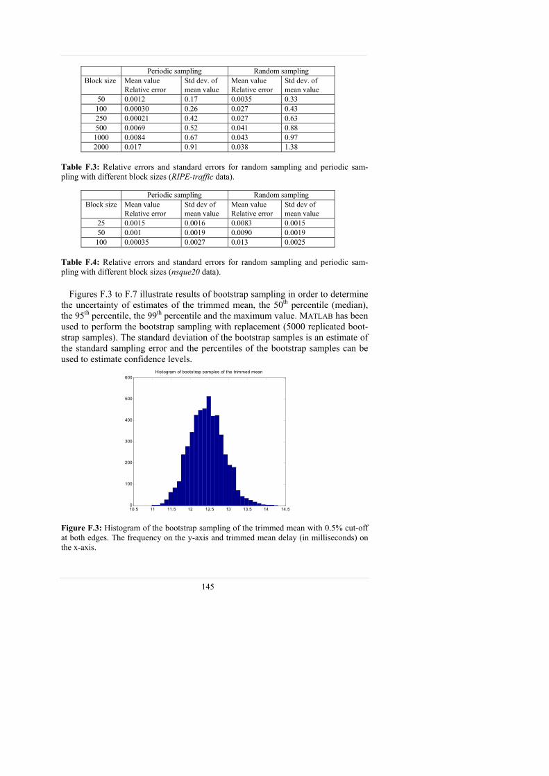
145

Periodic sampling Random sampling Block size Mean value

Relative error Std dev. of mean value

Mean value Relative error

Std dev. of mean value

50 0.0012 0.17 0.0035 0.33 100 0.00030 0.26 0.027 0.43 250 0.00021 0.42 0.027 0.63 500 0.0069 0.52 0.041 0.88 1000 0.0084 0.67 0.043 0.97 2000 0.017 0.91 0.038 1.38

Table F.3: Relative errors and standard errors for random sampling and periodic sam-pling with different block sizes (RIPE-traffic data).

Periodic sampling Random sampling

Block size Mean value Relative error

Std dev of mean value

Mean value Relative error

Std dev of mean value

25 0.0015 0.0016 0.0083 0.0015 50 0.001 0.0019 0.0090 0.0019 100 0.00035 0.0027 0.013 0.0025

Table F.4: Relative errors and standard errors for random sampling and periodic sam-pling with different block sizes (nsque20 data).

Figures F.3 to F.7 illustrate results of bootstrap sampling in order to determine

the uncertainty of estimates of the trimmed mean, the 50th percentile (median), the 95th percentile, the 99th percentile and the maximum value. MATLAB has been used to perform the bootstrap sampling with replacement (5000 replicated boot-strap samples). The standard deviation of the bootstrap samples is an estimate of the standard sampling error and the percentiles of the bootstrap samples can be used to estimate confidence levels.

10.5 11 11.5 12 12.5 13 13.5 14 14.50

100

200

300

400

500

600Histogram of bootstrap samples of the trimmed mean

Figure F.3: Histogram of the bootstrap sampling of the trimmed mean with 0.5% cut-off at both edges. The frequency on the y-axis and trimmed mean delay (in milliseconds) on the x-axis.

146

A histogram of bootstrap sampling of the trimmed mean value with 0.5% cut-off at both edges is shown in Figure F.3. The standard error estimate is 0.45. The mean value is 12.4 ms and the 95th percentile is 13.2 ms.

8.5 9 9.5 10 10.5 110

100

200

300

400

500

600Histogram of bootstrap sampling of the median

Figure F.4: Histogram of the bootstrap sampling of the median. The frequency on the y-axis and the delay median (in milliseconds) on the x-axis.

The mean value of the median bootstrap samples in Figure F.4 is 9.6 and the standard error is 0.35.

20 25 30 35

0

500

1000

1500Histogram of the bootstrap samples for the 95th percentile

Figure F.5: Histogram of the bootstrap sampling of 95th percentile. The frequency on the y-axis and the 95th percentile delay (in milliseconds) on the x-axis.

The histogram of the 95th percentile bootstrap sampling is shown in Figure F.5.

The standard error is 1.4. The 95th percentile of the bootstrap samples is 27.5 ms and the 99th percentile is 31.9 ms.

147

24 26 28 30 32 34 36 38 40 42

0

200

400

600

800

1000

1200

1400

1600

1800Histogram of the bootstrap samples for the 99th percentile

Figure F.6: Histogram of the bootstrap sampling of 99th percentile. The frequency on the y-axis and the 99th percentile delay (in milliseconds) on the x-axis.

The histogram of the 99th percentile bootstrap sampling is shown in Figure F.6. The standard error is 3.1. The 95th percentile of the bootstrap samples is 41.0 ms and the 99th percentile is 41.2 ms.

24 26 28 30 32 34 36 38 40 42

0

500

1000

1500

2000

2500

3000

3500Histogram of bootstrap samples of the maximum

Figure F.7: Histogram of the bootstrap sampling of the maximum value. The frequency on the y-axis and the maximum delay (in milliseconds) on the x-axis.

Figure F.7 shows a histogram of bootstrap sampling of the maximum value. The mean value is 38.6 ms and the standard deviation of the bootstrap samples (i.e. the standard error) is 3.3. It should be noted that the bootstrap technique not always produces reliable results for extreme values.

149

APPENDIX G

Performance Management in Switched ATM Networks

The following paper was presented at IS&N98 (Fifth International Conference on Intelligence in Services and Networks) in Antwerpen, May 1998. Telia Pro-soft (today TietoEnator) sponsored the work.

1. Introduction The current and expected introduction of more refined products in the tele-

communication networks, such as multimedia and other value-added services, means that management of broadband networks faces new challenges. Network operators offering services with specified guarantees for Quality of Service (QoS) accordingly have to monitor and control relevant network performance parameters. However, these management services will be carried out in a more dynamic and complex environment than today. Besides permanent connections, a signalling system that enables end-users to activate services on-demand is required when the number of users, the variety of services and the traffic load grow. In addition, to facilitate the introduction of value-added services in broad-band networks various kinds of architectures for service platforms have been discussed in recent years. Since capabilities to provide services with different levels of guarantees for QoS is a cornerstone in modern telecommunication sys-tems, flexible and effective methods to monitor and control parameters pertinent to network performance are unavoidable.

The purpose of this paper is to discuss these new conditions for management in the network and service domains, focusing on performance management in ATM networks. Besides a background to the issue, a general framework for perform-ance management in switched broadband networks is presented in Section 2, while the topic in the following section is QoS management from the perspective of a service platform. Section 4 is focused on in-service methods for monitoring of network performance parameters, especially cell losses, in the user plane in switched ATM networks. The approach adopted in this paper is believed to fa-cilitate solutions for performance management in a more complex environment than today.

150

2. Performance Management in Switched ATM Networks

Unlike Permanent Virtual Connections (PVCs) in current ATM networks, Switched Virtual Connections (SVCs) are configured dynamically on-demand by the end-users. These mechanisms, emerging in today’s networks, are imple-mented in the user-to-network interface based on standards such as UNI 3.1/4.0 (ATM Forum) and Q.2931 (ITU-T), and between network nodes based on proto-cols such as P-NNI, B-ISUP and B-ICI.

In future signalling systems, separation between call handling and connection handling is considered to increase flexibility, and to facilitate a more efficient distribution of resources within the network (see e.g. Magic [86], Expanse [87] and DPCA [88]). Moreover, the introduction of different service platforms in order to provide value-added services calls for some kind of session control (or “service signalling”) to handle the relation between the service logic and the resources in the connectivity networks used by the platform.

Performance monitoring of dynamically established VC (Virtual Channel) connections are difficult to manage for several reasons. The network manage-ment system may not be aware of when and where the connections are set up, and have no knowledge of the duration of the connections and the route taken throughout the network. These problems were recognised as open issues in a EURESCOM project [84] and were also addressed in a contribution to NOMS’96 [89].

Against this background, a framework for performance management in switched broadband networks, focusing on performance monitoring of the user plane in the ATM layer, is discussed in the following subsections. The main idea is that a close interaction between the call control functions and the management functions provides possibilities to differentiate performance monitoring of switched virtual connections. This has to be based on a policy that defines the aims and objectives for performance monitoring.

2.1 A Policy-Based Performance Management Service An overall performance management service, comprising monitoring, evalua-

tion and control, covers the user plane as well as the control plane (e.g. discussed at IS&N’95 by [90]). This section focuses on objectives for performance moni-toring of the user plane in ATM networks.

One obvious purpose is to support performance analysis of the network as a whole, a specific subnetwork or link. Another goal for performance monitoring is to verify the QoS offered to customers in traffic contracts or Service Level Agreements, which also might require translations of network parameters into QoS parameters. Unlike the traditional telephony network where every call ex-hibits similar performance characteristics, ATM networks enable integration of different service classes, which means that the QoS parameters vary for each individual call or connection. For that reason, operators and their customers have

151

an interest in performance reports that reveal more detailed information than merely general descriptions of the aggregated traffic on the links in the network. Hence, for monitoring purposes, a set of relevant network performance parame-ters, representing mainly loss of information and delays, has to be specified. An operator also has to decide whether end-to-end connections and/or certain seg-ments within the connections are meant to be monitored. Furthermore, the focus might be on all or certain service/traffic categories, or possibly on particular parameters in connections used by specific customers. The measurements needed for this variety of surveillance objectives are preferably carried out using in-service methods applied to the actual user traffic. One example of a measurement function is collection of samples of specified parameters from connections be-longing to specific service classes or from every connection belonging to certain links during a time interval. However, in order to achieve reliable and significant results in a cost-efficient way, a trade-off between continuous measurements and sampling has to be considered. Thus, performance monitoring functions include the pertinent network parameters (and threshold values), the entities (or domains) to be monitored such as links, connections and services, the method for monitor-ing (e.g. in-service methods) and the appropriate statistical methods to be used.

From a network provider’s point of view, it would be advantageous to specify the monitoring functions in terms of different monitoring policies (possibly for different domains), in order to hide implementation details and concentrate on the functional level. As the complexity of distributed, heterogeneous networks and services increases, the idea of policy-based management is becoming even more important for network operators (see e.g. [91] and [92]).

2.2 A General Model for Performance Monitoring in Switched ATM Networks

A general framework for performance management in switched ATM net-works has to include a model for interaction between what is referred to as the management plane and the control plane in the ATM reference model [93]. In-formation that the management system lacks concerning the dynamic behaviour of the connections is hidden in the call control system. These mechanisms (sig-nalling, routing, resource handling etc.) are in possession of the information needed to carry out performance monitoring such as when a session is being set up, the participants in the session and the route in the network. If data from the control plane and management plane is regarded as a common resource, this information base is available for the management functions as well. The question is rather if it is feasible to synchronise these functions from different domains and possibly different time scales, and how it can be implemented.

A general model for interaction between the management plane, consisting of plane and layer management in the switching systems, the network management system and the control plane functions is depicted in Fig. 1. The network man-agement system is responsible for the overall monitoring objectives throughout the network. The plane management functionality in the switching systems co-ordinates all management activities in a node, and handles the communication

152

with the central network management system. Performance monitoring of the ATM layer in the nodes is carried out by Layer Management and can be imple-mented using in-service methods, such as dedicated monitoring cells (further developed in Section 3).

The control system detects a pending service/call through the set-up message that comprises information about the end users, the service class, the QoS pa-rameters etc. Moreover, the control system carries information about the chosen route in the network and the bandwidth allocated for the connections being set up. The layer management system is notified and may, depending on the moni-toring policy, activate monitoring cells (or use other possible techniques) be-tween the endpoints of a connection or for segments along the connection. The collected information is then stored in a management information base super-vised by the network management system. However, this additional functionality provided by the above or similar models increases complexity and processor load in the systems as well.

Network Management System

Call Control Functions(signalling, routing etc.)

Plane & LayerManagement

in theSwitching Systems

Managementof controlfunctions

1. A pending call triggersOAM functions

2. OAM functions areactivated in accordance with

a monitoring policy

Monitoringpolicy and

reports

Fig. 1: Interaction between control functions and management functions. The network management system is responsible for the overall monitoring policy. Ac-tivation of OAM functions in the nodes in accordance with the monitoring policy is triggered by the signalling mechanism in the control plane.

The above reasoning assumes that the assignment of logical channels is not structured with respect to different service categories. In ATM networks, Virtual Path Connections (VPCs) provide convenient means of grouping similar Virtual Channel Connections (VCCs). This possibility often referred to as network re-source management [94], to separate traffic flows according to various service characteristics could facilitate performance monitoring. Co-ordination between performance management functions and network resource management and routing is a way to simplify monitoring of various service classes and groups of connections in the network. On the other hand, monitoring of SVCs requires synchronisation of call control and management functions as demonstrated ear-lier. A comparison between these two different but not excluding approaches is however a subject for a separate paper.

153

2.3 Interaction between the Management Plane and the Control Plane

As discussed in the previous section interaction between management and con-trol is a key issue in management of switched ATM networks. However, this integrated approach is not limited to performance monitoring. The ACTS project REFORM is an example of integration between fault management, resource management and control in ATM based networks. More specifically, the purpose is to integrate load balancing, OAM restoration, dynamic routing, and resource management [95].

Generally, there are obvious advantages in regarding data used by respectively control and management systems as parts of a common information base. As an example, the routing and signalling system P-NNI collects and uses information about faults and performance parameters throughout the network, while at the same time the performance management system collects similar data.

In recent years, architectures for providing services in telecommunication net-works as service platforms built on top of different connectivity networks have attracted considerable interest. In this context, management is often treated as an integrated and dynamic part of the telecommunication service. Configuration, alarm handling and other functional components are in that approach tied to the service through interfaces (e.g. according to a “pick and mix principle” [96]), which underlines the need for interaction between management functions and, in this case, service (session) control functions.

The xbind platform (a broadband kernel for multimedia services from CTR at the Columbia University, New York) has an architecture that integrates man-agement and signalling based on a common information structure [97]. Differ-ences regarding functionality, but also various real-time requirements, are the main reasons for a division of this framework into specific layers (information transport, connection management, resource control, and network management). Each function utilises a common information base, the Binding Interface Base (BIB), shared by the whole system via different interfaces.

3. Service Platforms and Performance Management Specific platforms in the service domain are evolving as tools for service pro-

viders to offer a wide range of value-added services to customers. These overlay service networks are meant to exploit mainly broadband networks for transporta-tion and connectivity, but also to support interworking with other existing tele-communication networks. The ability to deliver services with guarantees for specified levels of QoS is an essential property of a broadband service platform. In order to ensure these quality guarantees, a platform has to provide manage-ment services that enable the operators, and customers, to measure, monitor, analyse, control network performance and QoS, and relate this information to the services.

Since a service platform has an overlay character, performance management on the service level (QoS management) necessarily encompasses interaction with

154

not only the service (call) control functions in the service domain, but also with management and control functions in the connectivity networks (Fig. 2). The management system in the service domain is responsible for monitoring of the QoS goals, expressed as a monitoring policy in high-level service terms. Due to the dynamic nature of the service sessions, the management system is not aware of when a session is established, in which network or between which nodes the connections are set up. However, the service session control system that detects a pending service (call) holds information about the end users, the service class, the QoS parameters, the allocated bandwidth and routes in the connectivity net-work(s) etc. This interaction between control and management functions is of the same nature as discussed in Section 2. In addition, the monitoring policy in the service domain, expressed in terms of QoS, has to be translated into network performance parameters related to the bearer networks. Moreover, it implies a close interaction between management the signalling and routing functions in the connectivity networks. In an ATM network, this can be carried out using dedi-cated monitoring cells, as described in the next section, to measure for example delays and cell losses within connections used by specific service sessions. Ac-cordingly, the management system in the service domain is not only responsible for the overall principles guiding performance monitoring, but also for co-ordination of these functions between the service platform and the bearer net-works, and for storage and analysis of the measurement data.

Although performance parameters on the network level have significant impact on QoS for end-to-end services, a comprehensive QoS management system also has to include monitoring of higher levels such as the ATM adaptation layer, transport protocols and the application level. As the integration between tele-communication and information systems continue, a corresponding approach is necessary for performance management, which means that not only networks and network elements but also databases, servers and other systems have to be included.

Session & resource control in the service domain

Management system inthe service domain

Control functions inthe bearer network domain

Management system inthe bearer network domain

Fig. 2: Interaction between control functions and management functions in the service domain and the connectivity network domain.

155

4. An Infrastructure for In-Service Monitoring of the ATM Layer

A general model for performance management in switched broadband net-works and QoS management from the perspective of a service platform was discussed in the two previous sections. However, management services to achieve these goals are dependent on efficient methods to measure and monitor relevant performance parameters in the connectivity networks. The following section presents in-service methods as a feasible infrastructure for performance monitoring of ATM networks. These dedicated monitoring cells, periodically inserted between user cells, provide a mechanism for measurements that reflect relevant parameters in the actual user traffic.

4.1 In-Service Methods OAM cells, standardised by ITU-T [83], can be regarded as an infrastructure

for in-service monitoring of the ATM layer in the networks. ATM layer man-agement is co-ordinated and supervised by the overall plane management, which is responsible for other functional areas as well (fault, configuration, security and accounting management) in a switching system. Plane management also handles communication with the network management system, for example a TMN sys-tem using SNMP or CMIP over a Q-like interface ([93], [98] and [99]). Besides, in performance management, OAM cells are also defined for fault management.

On the Virtual Path level (the F4 flow) monitoring cells are identified by cer-tain reserved VCI (Virtual Channel Identifier) values, and on the Virtual Channel level (the F5 flow) the Payload Type Identifier (PTI) indicates whether a cell contains user data or OAM information. The F4 and F5 flows and surrounding layers are illustrated in Fig. 3.

AAL

ATM

P.L.

AAL

ATM

P.L.

AAL performance

I.610(OAM-principles)

(G.826)

F6

F5 (VC)F4 (VP)

F1-F3

Fig. 3: OAM performance principles for the ATM layer and surrounding layers.

The main idea is that OAM cells should experience the same conditions as the cells that carry user traffic. These monitoring cells are periodically inserted be-tween blocks of user cells as illustrated in Fig. 4. The length of the block size and the direction (forward monitoring and backward reporting) of the monitoring process are decided in the activation procedure. The format of the monitoring cell is shown in Fig. 5.

156

OAM cell OAM cell

Block of user cells (1024, 512, 256 or 128) Fig. 4: The average size of the monitoring blocks defined by ITU-T (the block size is permitted to vary 50% up or down from these nominal values).

In the forward direction, a Monitoring Cell Sequence Number (MCSN) keeps track of lost OAM cells. The Total User Cell Number (TUCN) is the number of ATM cells transmitted since the last OAM cell. A Block Error Detection Code (BEDC) is calculated over the preceding block and an optional time stamp can be inserted. In the backward reporting section, the Total Received Cell Count (TRCC) is indicated together with the result of the block error check. The moni-toring procedure can be defined between the endpoints (VPCs or VCCs) of the connection or for segments within the connection. Segment mode gives a possi-bility to delimit the source of performance deterioration along a connection.

Backward reportingForward monitoring

Cellheader

MCSN TUCN(CLP 0+1)

BEDC TUCN(CLP 0)

Timestamp

TRCC(CLP 0+1)

BLER TRCC(CLP 0)

Fig. 5: Format of the OAM cell according to I.610 (ITU-T) beginning with the cell header.

Keeping to the recommended format in I.610 the following parameters can be measured:

• Cell Error Ratio (CER); • Severely Errored Cell Block (SECB), which means more than M

errored cells or more than K lost or misinserted cells; • Cell Loss Ratio (CLR), where the case when the number of lost

cells equals the number of misinserted cells is interpreted as if no cell losses existed; and

• Cell Transfer Delay (CTD) and Cell Delay Variation (CDV), which requires some kind of synchronisation between the clocks in the switches.

The following section gives an example of a conceivable use of OAM cells for monitoring short-term parameters in the cell loss process, which has important implications for network performance and QoS.

4.2 Monitoring of the Cell Loss Process Cell losses in ATM networks are caused by several factors such as overflow in

the buffers, cell discards due to policing functions, misinserted cells and trans-mission errors. The cell loss ratio and the distribution of losses in time have an important impact on the quality-of-service for a large range of telecommunica-tion services. The behaviour of transport protocols like TCP (Transmission Con-

157

trol Protocol) are influenced by cell losses causing re-transmissions of packets and impaired performance. A well-known problem in monitoring of cell losses is the exceptionally long monitoring times needed to determine if a certain CLR limit has been reached.

The parameter CLR (Cell Loss Ratio) is a long-term average measure that does not reveal the short-term properties of the cell loss process. Several studies show that cell losses are not uniformly distributed but instead exhibit a bursty behav-iour that could be captured in terms of cell loss-free periods, cell loss periods and CLR for the loss bursts [100]. A cell loss period is defined as a block of cells beginning and ending with lost cells containing less than (or equal to) K con-secutive cells as shown in Fig. 6.

Information about these loss periods and loss-free periods is valuable and often more useful than the overall CLR measure. Murakami et al. have proposed an IPP (Interrupted Poisson Process) model in order to estimate parameters in the cell loss process using measurements provided by OAM cells [101]. A case study [81] based on real data traffic shows obvious deviations between estimated and expected values, especially for the length of the cell loss period. However, it is possible to define a measure that describes these periods in terms of the mean length of respectively the loss-free and the loss period, expressed in number of OAM blocks2. In addition, the cell loss ratio for the loss bursts (the relation be-tween lost cells and totally sent cells in the loss bursts) can also be given.

….

(less than K consecutive cells)

Loss period Loss-free period

Fig. 6: Definition of a cell loss period beginning and ending with lost cells (shaded) and containing less than (or equal to) K consecutive loss-free cells.

4.3 Interaction with Signalling For Permanent Virtual Connections (PVCs), OAM cells can be activated

through a management system when the PVC is configured. However, depending on the monitoring policy these configurations might have to be adjusted. A man-agement system should enable the network operator, or possibly a customer-based management system, to change the rules for activating monitoring cells.

On the other hand, a management system is not aware of when and where Switched Virtual Connections (SVCs) appear in the network. Thus, activation of OAM cells (a layer management function) has to be triggered by the signalling system (a call control function). This could for example be implemented using parameters in the signalling messages. When a call is being set up the decision whether monitoring cells are to be activated or not is made by the layer manage-

2 An OAM block consists of the number of user cells between two consecutive OAM cells.

158

ment system, based on the rules in the monitoring policy deployed in the network by the network management system as demonstrated in Section 2.1.

4.4 General Management Cells Besides these monitoring functions, Chen et al. recommend a broader defini-

tion of management cells carrying for example network state information (e.g. congestion levels, available bandwidth), control information (e.g. routing changes, bandwidth allocation) and administrative information (e.g. resource usage, encryption keys). The proposal can be viewed as an adjunct protocol defined for a special class of control packets similar to Internet Control Message Protocol (ICMP) messages in the Internet Protocol. Furthermore, Chen et al. suggest that intermediate nodes along a connection should have the ability to add information to the OAM cell. This extended function facilitates measurements of CTD/CDV (see Section 4.1) without clock synchronisation and a more detailed analysis of information collected along a connection that comprises several nodes [102]. A model for estimation of CDV and CTD without clock synchroni-sation has been put forward by Roppel exploiting round-trip measurements with OAM cells and a model for estimation of the differences between the clocks [103].

In the same spirit, Young-Il Kim et al. [104] suggest “a hybrid performance management scheme for OAM functions supporting QoS management in ATM networks”. In this proposal, a management system has the capability to switch between the F4 and F5 levels, and between end-to-end and segment monitoring modes in order to detect and analyse performance deterioration. Another model utilising an infrastructure of OAM cells based on intelligent agents for surveil-lance and control of congestion in ATM networks have been presented by Gaiti and Pujolle [105]. As mentioned in Section 4.2, Murakami et al. have used a model based on measurements provided by OAM cells in order to estimate pa-rameters in the cell loss process [101]. The above examples of further develop-ment of OAM cells indicate the need for more general-purpose mechanisms in ATM layer management.

5. Conclusions A general model for performance management, especially performance moni-

toring, in switched ATM networks based on interaction between different levels of management and control functions has been presented. This approach is be-lieved to facilitate solutions for performance management in a more complex environment than today. In this context, some components in a policy-based performance monitoring service, provided by the network management system, has been identified. Moreover, when service overlay platforms are introduced, a similar procedure is needed between the network and the service domains as well. Dedicated OAM cells are a feasible infrastructure for in-service monitoring of the actual user traffic that has potentials to be extended to more general-purpose management cells. As an example, the possibility to derive valuable information about the short-term characteristics of the cell loss process using in-

159

service methods is illustrated in the paper. Since capabilities to provide services with different levels of guarantees for QoS is a cornerstone in modern telecom-munication systems, flexible and effective methods to monitor and control pa-rameters pertinent to network performance are unavoidable.

161

APPENDIX H

Methods and Models for In-Service Monitoring and Estimation of Cell Losses in ATM Networks

The following paper was presented at ICT98 (International Conference on Telecommunications) in Porto Carras, Greece, in June 1998. Telia Prosoft (today TietoEnator) sponsored the work.

1. Introduction The current and expected introduction of more refined products in the tele-

communication networks, such as multimedia and other value-added services, means that management of broadband networks faces new challenges. The need for Quality of Service (QoS) guarantees is a growing trend amongst public broadband network operators as well in the Internet community. Unlike tradi-tional telecommunication networks today’s broadband technology integrates a wide range of services, each with possibly different QoS obligations. However, since ATM technology is based on packet mode in order to increase efficiency, the network performance characteristics are not deterministic, uniform or static with respect to services, connections and different time-periods. Performance parameters in fast packet networks, such as information losses and delays, are clearly decisive for the final QoS experienced by the end-users. Accordingly, performance management (comprising monitoring, analysis and control) requires more differentiated methods than prevalent in the traditional networks. In ATM networks monitoring of relevant parameters in the actual user traffic can be per-formed via dedicated OAM cells

Cell losses are one of the main sources of performance deterioration in ATM networks. The purpose of this paper is to examine possibilities to monitor and estimate the short-term behaviour of the cell loss process exploiting in-service methods, as a complement to the more general and often less informative long-term Cell Loss Ratio (CLR). In previous research, different models for estima-tion of these short-term parameters in the cell loss process, mostly supported by simulations, have been suggested. The approach in this paper is to examine one of these models using representative real traffic data (provided by Telia), and based on the results in this case study evaluate the potentials of in-service moni-toring methods for estimation of the cell loss process.

In the remainder of Section 1 the concept of OAM cells is presented, followed by a review of subsequent developments in this field. In Section 2 models for estimation of parameters, such as the mean size of the cell loss periods and loss-free periods are analysed and tested against real traffic data. A new, alternative measure of these parameters expressed in terms of OAM blocks is considered in

162

Section 3. An alternative technique is also mentioned, followed by a summary in Section 4.

1.1 In-Service Monitoring Using OAM Cells OAM cells, standardised by ITU-T [83], can be regarded as an infrastructure

for in-service monitoring of the ATM layer in the networks. Besides perform-ance management, OAM cells are also defined for fault management. On the Virtual Path level (the F4 flow) monitoring cells are identified by certain re-served VCI (Virtual Channel Identifier) values, and on the Virtual Channel level (the F5 flow) the Payload Type Identifier (PTI) indicates whether a cell contains user data or OAM information.

The main idea is that OAM cells should experience the same conditions as the cells that carry user traffic. These monitoring cells are periodically inserted be-tween blocks of user cells as illustrated in Fig. 1.

OAMll

OAMll

Block of user cells (1024, 512, 256 or 128)

Fig. 1: The average size of the monitoring blocks defined by ITU-T (the block size is permitted to vary 50% up or down from these nominal values).

The length of the block size and the direction (forward monitoring and back-ward reporting) of the monitoring process are decided in the activation proce-dure. The format of the monitoring cell is shown in Fig. 2.

In the forward direction, a Monitoring Cell Sequence Number (MCSN) keeps track of lost OAM cells. The Total User Cell Number (TUCN) is the number of ATM cells transmitted since the last OAM cell. A Block Error Detection Code (BEDC) is calculated over the preceding block and an optional time stamp can be inserted. In the backward reporting section, the Total Received Cell Count (TRCC) is indicated together with the result of the block error check.

unused TRCC0

BLER TRCC0+1

Reserved EDC….

Backward reporting

Cellheader 0010 Function

type MCSN TUCN0+1

BEDC TUCN0

Timestamp

...

Forward monitoring

Fig. 2: The format of the OAM cell used for performance monitoring, starting with the cell-header at the left.

The monitoring procedure can be defined between the endpoints of the connec-tion (VPC or VCC) or for segments within the connection. Segment mode gives a possibility to delimit the source of performance deterioration along a connec-

163

tion. According to the recommendation I.610 the following parameters can be measured:

• Cell Error Ratio (CER); • Severely Errored Cell Blocks (SECB), which means more than M

errored cells or more than K lost or misinserted cells; • Cell Loss Ratio (CLR), where the case when the number of lost

cells equals the number of misinserted cells is interpreted as if no cell losses existed; and

• Cell Transfer Delay (CTD) and Cell Delay Variation (CDV). This requires some kind of synchronisation between the clocks in the switches.

1.2 General-Purpose Management Cells Besides these monitoring functions, Chen et al. recommend a broader defini-

tion of management cells carrying for example network state information (e.g. congestion levels, available bandwidth), control information (e.g. routing changes, bandwidth allocation) and administrative information (e.g. resource usage, encryption keys). The proposal can be viewed as an adjunct protocol defined for a special class of control packets similar to Internet Control Message Protocol (ICMP) messages in the Internet Protocol. Furthermore, Chen et al. suggest that intermediate nodes along a connection should have the ability to add information to the OAM cell. This extended function facilitates measurements of CTD/CDV without clock synchronisation and a more detailed analysis of infor-mation collected along a connection that comprises several nodes [102]. A model for estimation of CDV and CTD without clock synchronisation has been put forward by Roppel exploiting round-trip measurements with OAM cells and a model for estimation of the differences between the clocks [103].

In the same spirit, Young-Il Kim et al. [104] suggest a “hybrid performance management scheme for OAM functions supporting OoS management in ATM networks”. In this proposal, a management system has the capability to switch between the F4 and F5 levels, and between end-to-end and segment monitoring modes in order to detect, delimit and analyse performance deterioration. Another model, which also uses OAM cells as an infrastructure, based on intelligent agents for surveillance and congestion control in ATM networks has been pre-sented by Gaiti and Pujolle [105]. The above examples of further development of OAM cells indicate the need for more general-purpose mechanisms in ATM layer management. The next section focuses on measurement and estimation of the cell loss process, which is one of the dominating sources behind performance deterioration in ATM networks.

2. Estimation of Short-Term Parameters in the Cell Loss Process

Cell losses in ATM networks are mainly caused by overflow in buffers but also by cell discards due to policing functions, misinserted cells and transmission

164

errors. The impact of cell losses on the QoS is considerable for a large range of telecommunication services. For example the behaviour of transport protocols such as TCP are influenced by cell losses causing re-transmissions of packets and impaired performance.

For a cell loss ratio of 10-8 and an average bit rate of 1.5 Mb/s, the mean inter-val between consecutive cell losses is almost eight hours, and around three sec-onds for a 135 Mb/s connection and CLR=10-6. However, several studies show that cell losses are not uniformly distributed but instead exhibit a bursty behav-iour that could be captured in terms of cell loss-free periods, cell loss periods and CLR for the loss bursts [100]. The parameter CLR is a long-term average meas-ure that does not reveal the short-term properties of the cell loss process. A cell loss period is defined as a block of cells beginning and ending with lost cells containing less than (or equal to) K consecutive cells, as shown in Fig. 3.

….

(less than K consecutive cells)

Loss period Loss-free period

Fig. 3: Definition of a cell loss period beginning and ending with lost cells (shaded) and containing less than (or equal to) K consecutive loss-free cells.

The interrupted Poisson process (IPP), which is used in several studies to model the bursty nature of the cell loss process, was originally presented by Kuczura (1973) to describe overflow traffic in the telephony network [106]. This model or the discrete counterpart IBP (interrupted Bernoulli process), can be seen as a special case of a Markov modulated Poisson process primarily utilised to model traffic sources (see e.g. [107] and [108]).

The IPP model represents a Poisson process that is turned on for an exponen-tially distributed period of time (active or busy period) and turned off for another exponentially distributed period of time (silent period). In this case, the active periods correspond to cell loss bursts, and the silent periods correspond to loss-free periods. The inter-arrival distances between losses within the cell loss peri-ods are also assumed to be exponentially distributed. For the IBP model, which is a discrete version of IPP, these periods are geometrically distributed. Let 1/α and 1/β denote the average duration of the active (loss) period and the silent (loss-free) period and let λ denote the loss-generating rate during a loss period. The probability distributions are then given by:

Pr{X≤t}=1-e-αt ; Pr{Y≤t}=1-e-βt ; Pr{Z≤t}=1-e-λt.

2.1 Monitoring and Measurement Scenarios Two possible cases of performance monitoring scenarios are illustrated in the

measurements presented below. The first measurement (performed on Telia’s commercial ATM network) represents a case where a permanent virtual connec-tion (PVC) is configured for typical LAN traffic, and utilises the remaining ca-

165

pacity on a link that carries CBR (Constant Bit Rate) traffic. LAN traffic be-tween two routers has been recorded during 24 hours as shown in Fig. 4 [109].

+

Router Router

CBR traffic

Analysis tools Fig. 4: LAN traffic measurement. The buffer with CBR traffic is given priority in the multiplexing process.

Before entering the buffer (size=630 cells) sequence numbers and time stamps are assigned to the cells. The average rate of the user traffic is 1.6 Mb/s and the peak rate is 9 Mb/s during the 24-hour period. This traffic is multiplexed together with CBR traffic (from a generator) that could be chosen arbitrary in order to achieve a desired level of cell loss ratio. The CBR traffic, that passes a separate buffer, is given priority which in this loaded case results in a cell loss ratio in the order of 5×10-5 for the recorded data traffic (and an equivalent bandwidth of 23400 cps). If the cell losses were uniformly distributed the time interval be-tween two consecutive losses would be approximately 0.9 seconds. However, the fact that cell losses appear in bursts is not evident from the overall CLR measure.

While the first case represents typical LAN traffic, the second measurement that was performed on Stockholm Gigabit Network concerns video traffic [110]. Cell losses from VBR video traffic (cell B coded Sun video) and CBR back-ground traffic that use a common buffer were recorded during half an hour. In both measurements, instruments developed in the RACE project PARASOL were used.

2.2 The Cell Loss Measurements The short-term parameters of the cell loss process from the measurement data

were analysed using MATLAB® and MATEMATICA®. The statistical properties of the size of the cell loss periods, the cell loss-free periods and the distances be-tween losses in the loss period were studied for K=32, 64, 128, 256, 512 and 1024 cells (in accordance with the definition illustrated in Fig. 4). In Fig. 5-8 the histograms of these periods (for K=32) from the 24 hours measurement of data traffic are shown. The distribution of the length of the loss period (Fig. 5) exhib-its a general shape that resembles the exponential distribution, while the histo-grams of the loss-free period (Fig. 6-7) seem more akin to the H2 distribution. The loss-free periods contain rare events of great magnitude (1.2×108 cells) while the main part of the loss-free periods are substantially lower (75% of the loss-free periods are shorter then 1600 cells). The ratio between the mean length of

166

the loss-free period and the mean length of the loss period is around 10000:1 for K=32 cells and 4300:1 for K=1024 cells. Fig.8 shows that in approximately 95% of the all cases the distance between losses in a loss burst is one or two cells.

A comparison between the exponential distribution and statistical data for these periods shows that the duration of the loss period is accepted as an expo-nential probability distribution according to the χ2

0.05 test for K=32, 64, 128, and 256 cells, and rejected on the 5% level for K=512 and K=1024. When K in-creases, the number of loss periods is reduced and the distribution loses more and more of its exponential nature. The hypothesis that the loss-free period and the distance between losses in the loss period behave according to an exponential probability distribution was rejected on a 5% risk level according to the χ2 test for all values of K. The loss-free period is probably approximated better by the H2 distribution. In the second measurement of cell losses (from traffic consisting of video sessions and CBR background traffic), the histograms of the loss-free and the loss periods exhibit properties that resemble the exponential distribution in both cases.

0 100 200 300 400 500 600 700 800 900 1000

0

0.02

0.04

0.06

0.08

0.1

0.12

0.14

0.16

0.18Distribution of the loss period

Number of cells in a loss period

Rel

ative

freq

uenc

ies

Fig. 5: Histogram of the length of the loss period, K=32. The mean value is 121 cells and the standard deviation, σ=125.

167

0 2 4 6 8 10 12

x 107

0

0.1

0.2

0.3

0.4

0.5

0.6

0.7

0.8

0.9

1Distribution of the loss-free period

Rel

ative

freq

uenc

ies

Number of cells in a loss-free period Fig. 6: Histogram of the length of the loss-free period, K=32. The mean value is 1.2×106 cells and the standard deviation, σ=8.6×106.

0 200 400 600 800 1000 1200 1400 1600

0

0.01

0.02

0.03

0.04

0.05

0.06

0.07

0.08Distribution of the length of the loss-free period

Rel

ative

freq

uenc

es

Number of cells in a loss-free period

Fig. 7: The first part of the distribution of the length of the loss-free periods in Fig. 6. (75% of the events). As seen in Fig. 6 the tail stretches up to 1.2×108.

0 5 10 15 20 25 30 35

0

0.1

0.2

0.3

0.4

0.5

0.6

0.7

0.8

Number of cells between losses in a loss period

Rel

ative

freq

uenc

ies

Distribution of the loss-free periods in a loss period

Fig. 8: Histogram of the inter-arrival distances between losses in the loss period, K=32. The mean value is 1.7 cells and the standard deviation, σ=2.6.

168

However, none of the loss or the loss-free periods was accepted as an exponen-tial distribution on the 5% risk level in the χ2 tests. Compared to the former case with LAN traffic the ratio between the lengths of the loss-free periods and the loss periods are substantially lower, 20:1 for K=32 cells and 2:1 for K=1024 cells.

2.3 Estimation of Short-Term Parameters in the Cell Loss Process Using OAM Cells

A prerequisite for the statistics presented above is access to special test meas-urement equipment, something that is not feasible for extensive performance management of entire networks. As demonstrated in Section 1.1 an infrastructure of dedicated OAM cells is a possible method for monitoring of ATM networks. Amongst others, Murakami et al. have presented a method for estimation of the short-term parameters in the cell loss process that uses OAM cells. Simulations of multiplexed voice and data transmissions ([101], [104]) support this method, based on the interrupted Poisson process. In our study, the above method has been applied to the cell loss measurements presented in Sections 2.1-2.2. The question is how well the short-term parameters in the cell loss process can be estimated by means of monitoring cells and a model-based approach.

In [101], a relationship between the probability of a single cell loss OAM block3 and the mean length of the cell loss period is presented. The prerequisite is still that the cell loss process acts according to an interrupted Poisson (or Ber-noulli) process (with alternating exponentially/geometrically distributed loss periods and loss-free periods). Given certain input data from the measurements (the number of lost cells, sent cells, loss bursts and also the number of OAM blocks that contain exactly one loss burst), the mean duration of the loss period and of the loss-free period as well as CLR for the loss bursts can de estimated. The result from the estimation of the short-term parameters in the cell loss proc-ess originating from the LAN traffic measurement is summarised in Table 1.

The estimation of the mean length of the loss period is quite uncertain with relative errors ranging from 1% up to 55% compared to the actual measured values. Since the mean length of the loss-free period is considerably longer, the relative errors become small. In the second measurement (video and CBR traffic) the relative errors concerning the duration of the loss period range from below 1% to 18%, and from below 1% to 5% for the loss-free periods.

3 i.e. the ratio between the events when a loss burst is completely enclosed between two consecutive OAM cells (an OAM block) and all loss bursts. The largest number of consecutive cells between lost cells (K) in a loss burst in this model is equal to the length of the OAM block.

169

OAM BLOCK (CELLS)

LOSS PERIOD (CELLS)

LOSS-FREE PERIOD (CELLS)

CLR WITHIN CELL LOSS PERIODS

1024 1300/839 (55%)

3.55×106/3.64×106 (2%)

0.17/0.26 (35%)

512 435/423 (3%)

2.60×106/2.65×106 (2%)

0.37/0.38 (3%)

256 285/293 (3%)

2.18×106/2.21×106 (1%)

0.47/0.46 (2%)

250/203 (23%)

1.76×106/1.80×106 (2%)

0.44/0.54 (19%)

Table 1: The mean length of the cell loss period and the loss-free period, and CLR for the loss period. The format is “estimated/measured” values with the relative error in brackets.

However, a prerequisite for the model is that the number of loss periods is measured accurately. The results shown in Table 1 are obtained from the true (measured) number of loss periods. In fact, it is not feasible to measure exactly the number of loss bursts via monitoring cells. The reason is that OAM cells are not aware of where in the monitoring block the lost cells were located. Consider the following event: a loss period ends in the beginning of one OAM block and (K or more cells ahead) a new loss period begins in the next OAM block. Al-though two different loss periods actually have occurred, only one loss period will be detected and registered. Hence, the method will underestimate the actual number of loss bursts4, which results in additional errors. Using these values measured by OAM cells, in the estimation of the mean length of the loss-free period will result in relative errors that range from 10% to 35%.

3. Evaluation and Results There are mainly two different obstacles in estimating the short-terms parame-

ters in the cell loss process. First, the statistical behaviour of the cell loss process in the studied material is not always in accordance with the exponential distribu-tion, which is required by the applied model. Especially this seems to be the case for the length of the loss-free period in the LAN measurement, but also regarding the length of the loss period when K is large. These deviations from the model assumptions probably explain the relatively high errors in estimating the mean length of the cell loss period. If the loss-free periods are considerably longer than the loss periods, the relative errors concerning the loss-free periods become rather small. Hence, if the ratio between the lengths of these periods is high, the model seems to produce reasonable estimations of the mean size of the loss-free period, even though the statistical prerequisites are not fulfilled. It seems, how-ever, that the cell loss process in the LAN traffic case is too complex for the IPP model to handle with stable and accurate results.

4 In this study the estimated number of loss bursts, using OAM cells, is 16% (in mean) beneath the measured value.

170

The second obstacle concerns the limitations in feeding the model with correct input data. Although OAM cells are suitable for monitoring of the user traffic in many respects, they are however not able to count the actual number of cell loss periods (which is necessary input data for the model). Although it might be pos-sible to improve the method and to obtain a better approximation of the number of loss bursts, the fundamental shortages remain. For that reason, it seems appro-priate to consider alternative ways to approach the problem as well.

3.1 A New Measure Based on OAM Blocks A new measure of the relevant parameters in the cell loss process using OAM

cells as an infrastructure for measurements can be defined in terms of the size of the monitoring block (the number of user cells between two consecutive OAM cells). The length of the cell loss period can be expressed as the number of con-secutive OAM blocks that contain lost cells. In the same manner, the length of the loss-free period can be expressed in terms of the number of consecutive OAM blocks without any lost cells in the payload. The cell loss ratio for the loss bursts (CLRB) is accordingly defined as the ratio between lost cells and totally sent cells in those OAM blocks that constitute the loss period. In a way this measure is similar to SES and SECB regarding bit errors5. The number of con-secutive OAM blocks for each period can be measured directly and the estima-tion procedure is no longer needed. The mean length of the loss-free period in the LAN traffic case is 4741 OAM blocks (σ=16158) and the number of loss periods is 60 during the 24-hour monitoring period (with OAM blocks of 1024 cells). The mean length of the loss period is 2.5 OAM blocks (σ=2.1) and CLRB=0.12 (CLR=5×10-5). Additional valuable information about the distribu-tion of these parameters can be obtained from Fig. 9-11 for further statistical analysis. This new proposed measure differs from the former definition of a loss period (in Section 2) in some respects.

1 2 3 4 5 6 7 8 9

0

0.05

0.1

0.15

0.2

0.25

0.3

0.35

0.4

0.45

Rel

ative

freq

uenc

ies

Number of OAM blocks in loss periods

Distribution of the duration of loss periods

Fig. 9: Histogram of the length of the cell loss period expressed in number of OAM blocks (1024 cells). The mean value is 2.5 OAM blocks.

5 SES is Severely Errored Seconds and SECB is Severely Errored Cell Blocks.

171

0 2 4 6 8 10 12

x 104

0

0.1

0.2

0.3

0.4

0.5

0.6

0.7

0.8Distribution of the duration of loss-free period

Number of OAM blocks in the loss-free period

Rel

ative

freq

uenc

ies

Fig. 10: Histogram of the distribution of the length of the loss-free period expressed in number of OAM blocks (1024 cells). The mean value is 4741 OAM blocks.

0 100 200 300 400 500 600

0

0.01

0.02

0.03

0.04

0.05

0.06

0.07

0.08

0.09

0.1Distribution of the number of lost cells in OAM blocks

Rel

ative

freq

uenc

ies

Number of lost cells in OAM blocks in cell loss periods Fig. 11: Histogram of the number of lost cells in OAM blocks (1024 cells) in cell loss periods. The mean value is 121 cells.

As previously explained it is not possible to trace the positions in the OAM block that the lost cells occupied, which explains why a number of relatively small loss-free periods are not detected. Since the lost cells are not uniformly distributed over the entire OAM block, the actual size of a loss period is often shorter than the OAM block (Fig. 11). Altogether, this means that the proposed method will underestimate the number of periods (loss periods as well as loss-free periods) and overestimate the mean size of both periods compared to the former definition of a loss period in Section 2. However, these differences decrease if the size of the OAM block is shorter.

Considering the demonstrated shortages of the model-based estimation of short-term parameters of the cell loss process this proposal to express those periods in terms of the number of consecutive OAM blocks seems robust and useful. In future work it is feasible to improve further the measure through

172

statistical analysis of the distributions exemplified in Fig. 9-11, but also in examining alternative techniques.

3.2 Other Techniques A well known problem in monitoring cell losses under normal conditions in

the network (not as loaded as the cases in this study) is the exceptionally long measurement times often needed to determine whether a certain limit of the cell loss ratio has been reached or not. One method to overcome the problem, discussed in several papers, is to monitor the arrival process. This approach utilises the linear relationship between the buffer size and the logarithm of the CLR. The method is valid for markovian sources and also for more general conditions ([111] and [112]). Small virtual buffers are used to detect CLR in the order of say 10-2-10-3 and these results can then be extrapolated to the ac-tual size of the physical buffer, which considerably shortens the monitoring times. Since buffer management techniques, such as per VC-queuing, are emerging for ATM switches this method for CLR monitoring might be ex-tended to handle separate connections as well as aggregated traffic.

4. Conclusions The need for Quality of Service (QoS) guarantees is a growing trend

amongst public broadband network operators as well in the Internet commu-nity. One of the main sources of performance deterioration in ATM networks is cell loss. The bursty nature of the cell loss process, illustrated in the paper by statistics from measurements of data and video traffic, is not clear from the overall CLR measure. This contribution has focused on in-service methods and statistical models for monitoring and estimation of these short-term parameters in the cell loss process. The study shows that estimation, based on an IPP model, of the length of the loss-free and loss periods using OAM cells exhibit quite uncertain results. There are mainly two reasons. First, the inability of OAM cells to measure necessary parameters (such as the exact number of loss bursts), and secondly the deviation of the cell loss process in the studied traffic data from the required exponential distribution of the length of the loss-free and the loss periods. Considering these shortcomings, a new measure of the mean size of these periods, based on monitoring cells and expressed solely in terms of the number of consecutive OAM cells that these periods comprise, is suggested.

performance monitoring in communication networks

Documents