performance modelling of an open volumetric receiver csp

Performance Modelling of an Open Volumetric Receiver CSP Plant Incorporating Rock Bed

Thermal Storage

by Jean-François Philippe Pitot de la

Beaujardiére

Dissertation presented for the degree of Doctor of Philosophy in the Faculty of Engineering at Stellenbosch University

Supervisor: Prof TW von Backström Co-supervisor: Prof HCR Reuter

April 2019

ii

General Declaration

By submitting this thesis electronically, I declare that the entirety of the work contained therein is my own, original work, that I am the sole author thereof (save to the extent explicitly otherwise stated), that reproduction and publication thereof by Stellenbosch University will not infringe any third party rights and that I have not previously in its entirety or in part submitted it for obtaining any qualification.

This dissertation includes three original papers published in peer-reviewed journals or books and one unpublished publication. The development and writing of the papers (published and unpublished) were the principal responsibility of myself and, for each of the cases where this is not the case, a declaration is included in the dissertation indicating the nature and extent of the contributions of co-authors.

Signature of candidate:

Date: April 2019

Copyright © 2019 Stellenbosch University

All rights reserved

Stellenbosch University https://scholar.sun.ac.za

iii

Plagiarism Declaration

1. Plagiaat is die oorneem en gebruik van die idees, materiaal en anderintellektuele eiendom van ander persone asof dit jou eie werk is.Plagiarism is the use of ideas, material and other intellectual property ofanother’s work and to present is as my own.

2. Ek erken dat die pleeg van plagiaat 'n strafbare oortreding is aangesien dit‘n vorm van diefstal is.I agree that plagiarism is a punishable offence because it constitutes theft.

3. Ek verstaan ook dat direkte vertalings plagiaat is.I also understand that direct translations are plagiarism.

4. Dienooreenkomstig is alle aanhalings en bydraes vanuit enige bron(ingesluit die internet) volledig verwys (erken). Ek erken dat diewoordelikse aanhaal van teks sonder aanhalingstekens (selfs al word diebron volledig erken) plagiaat is.Accordingly all quotations and contributions from any source whatsoever(including the internet) have been cited fully. I understand that thereproduction of text without quotation marks (even when the source iscited) is plagiarism.

5. Ek verklaar dat die werk in hierdie skryfstuk vervat, behalwe waar andersaangedui, my eie oorspronklike werk is en dat ek dit nie vantevore in diegeheel of gedeeltelik ingehandig het vir bepunting in hierdiemodule/werkstuk of ‘n ander module/werkstuk nie.I declare that the work contained in this assignment, except otherwisestated, is my original work and that I have not previously (in its entirety orin part) submitted it for grading in this module/assignment or anothermodule/assignment.

JFP Pitot de la Beaujardiére

Voorletters en van / Initials and

surname

April 2019

Datum / Date


iv

Publication Declarations

Publication 1

Declaration by the candidate: With regard to the journal article presented in Chapter 2, the nature and scope of my contribution were as follows:

Nature of contribution Extent of contribution (%) Development of research content, manuscript writing

80

The following co-authors have contributed to Chapter 2:

Name e-mail address Nature of Contribution

Extent of contribution (%)

HCR Reuter [email protected] Research oversight, technical guidance and manuscript editing

20


Date: April 2019

Declaration by co-authors: The undersigned hereby confirm that

1. the declaration above accurately reflects the nature and extent of thecontributions of the candidate and the co-authors to Chapter 2,

2. no other authors contributed to Chapter 2 besides those specified above, and3. potential conflicts of interest have been revealed to all interested parties and

that the necessary arrangements have been made to use the material inChapter 2 of this dissertation.

Signature Institutional Affiliation Date Declaration with signature in possession of candidate and supervisor

Stellenbosch University April 2019


v

Publication 2

Declaration by the candidate: With regard to the journal article presented in Chapter 3, the nature and scope of my contribution were as follows:

Nature of contribution Extent of contribution (%) Development of research content, manuscript writing

70

The following co-authors have contributed to Chapter 3:

Name e-mail address Nature of Contribution

Extent of contribution (%)

HCR Reuter [email protected] Research oversight, technical guidance and manuscript editing

10 SA Klein [email protected] 10 DT Reindl [email protected] 10


Date: April 2019

Declaration by co-authors: The undersigned hereby confirm that

1. the declaration above accurately reflects the nature and extent of thecontributions of the candidate and the co-authors to Chapter 3,

2. no other authors contributed to Chapter 3 besides those specified above, and3. potential conflicts of interest have been revealed to all interested parties and

that the necessary arrangements have been made to use the material inChapter 3 of this dissertation.



Declaration with signature in possession of candidate and supervisor

University of Wisconsin-Madison

April 2019


University of Wisconsin-Madison

April 2019


vi

Publication 3 Declaration by the candidate: With regard to the journal article presented in Chapter 4, the nature and scope of my contribution were as follows: Nature of contribution Extent of contribution (%) Development of research content, manuscript writing

80

The following co-authors have contributed to Chapter 4: Name e-mail address Nature of

Contribution Extent of contribution (%)

HCR Reuter [email protected] Research oversight, technical guidance, manuscript editing

10 TW von Backström

[email protected] 10

Signature of candidate: Date: April 2019 Declaration by co-authors: The undersigned hereby confirm that

1. the declaration above accurately reflects the nature and extent of the contributions of the candidate and the co-authors to Chapter 4,

2. no other authors contributed to Chapter 4 besides those specified above, and 3. potential conflicts of interest have been revealed to all interested parties and

that the necessary arrangements have been made to use the material in Chapter 4 of this dissertation.






vii

Abstract

Open volumetric receiver (OVR) concentrating solar power (CSP) plant technology utilises air as a heat transfer fluid, which enables higher peak power cycle temperatures in comparison to conventional heat transfer fluids. This creates the potential for improvements in solar-electric conversion efficiency and reduced electricity generation costs. Despite the promise of the technology, it still faces appreciable technical challenges that have inhibited its commercial adoption.

R&D activities have enabled progress in overcoming these challenges. However, a deeper understanding of plant behaviour is required to improve the competitiveness of the technology. In this regard, computational performance modelling at a system and plant level has served as a powerful tool for the exploration of new concepts and the evaluation of improved plant arrangements. Yet little attention has been paid to performance optimisation, and there is still a fairly limited understanding of plant performance characteristics.

The objective of this work is to develop a comprehensive plant modelling capability to enable further investigation of key aspects of OVR CSP plant operational behaviour. Of particular interest is the investigation of component inter-dependencies and the sensitivity of plant performance to variations in design parameters at a system and plant level.

Firstly, a comprehensive review of performance modelling studies associated with OVR CSP plant technology is presented, detailing recent developments in the simulation of open volumetric receivers, packed bed thermal energy storage systems and OVR CSP plants. The review establishes the state-of-the-art in modelling methodologies, evaluates the extent to which system and plant performance have been investigated, and identifies aspects of plant design and behaviour that require further attention.

A design-point model of a 100 MWe OVR CSP plant is then developed and applied to parametrically study the sensitivity of plant performance to heat recovery steam generator (HRSG) configuration and design parameters. The study provides novel insight into the thermodynamic interaction that exists between OVR and HRSG, and identifies the HRSG characteristics that permit the best utilisation of solar energy.

The effectiveness of the local thermal equilibrium (LTE) assumption in the long-term performance modelling of rock bed thermal energy storage systems is then evaluated. A one-dimensional LTE performance model is formulated and validated, and applied to simulate the annual performance of a CSP rock bed. Predictions are compared to those associated with an analogous two-phase model to establish, for


viii

the first time, the applicability of the LTE assumption for the conditions typically associated with air-rock CSP packed beds. Finally, a detailed OVR CSP plant model with off-design fidelity is developed and applied to parametrically study the long-term performance of a 100 MWe plant, incorporating rock bed thermal energy storage and operating in a peaking role. In this manner, the annual performance of a plant of this configuration is predicted for the first time. Furthermore, the relationships between plant solar-electric efficiency, energy yield, heliostat field size and thermal energy storage capacity are detailed.


ix

Opsomming Oop volumetriese ontvanger (OVO) konsentrasie sonkrag (KSK-) aanlegtegnologie gebruik lug as ŉ warmteoordragsvloeistof, wat hoër kragopwekkingskringloop-temperature moontlik maak in vergelyking met konvensionele warmteoordrags-vloeistowwe. Dit skep die potensiaal vir verbeteringe in son-elektriese omsettingsdoeltreffendheid en verlaagde elektrisiteitsopwekkingskoste. Ondanks die belofte wat die tegnologie inhou, kom dit steeds voor aanmerklike tegniese uitdagings te staan wat die kommersiële implementering daarvan belemmer. Aktiwiteite in navorsing en ontwikkeling het vordering ten opsigte van oorkoming van hierdie uitdagings moontlik gemaak. ŉ Meer diepgaande begrip van aanleggedrag is egter nodig om die mededingendheid van die tegnologie te verbeter. In hierdie opsig het rekenaarverrigtingmodellering op stelsel- en aanlegvlak as ŉ sterk instrument gedien vir die verkenning van nuwe konsepte en die evaluering van verbeterde aanlegopstellings. Tog word min aandag gegee aan die optimalisering van verrigting, en is daar steeds redelik beperkte begrip van aanlegverrigtingeienskappe. Die doelstelling van hierdie studie was om ŉ omvattende aanlegmodelleringvermoë te ontwikkel om verdere ondersoek van sleutelaspekte van OVO KSK-aanlegbedryfsgedrag moontlik te maak. Die ondersoek van komponente se onderlinge afhanklikheid en die sensitiwiteit van aanlegverrigting vir verskille in ontwerpparameters op stelsel- en aanlegvlak was van besondere belang. Eerstens word ŉ omvattende oorsig van verrigtingmodelleringstudies verbonde aan OVO KSK-aanlegtegnologie aangebied, waarin onlangse ontwikkelinge in die simulasie van OVO’s, gepakte bed termiese energiebergingstelsels en OVO KSK-aanlegte in besonderhede bespreek word. In die oorsig is die ultramoderne modelleringsmetodologieë bepaal, die mate waarin stelsel- en aanlegverrigting ondersoek is, geëvalueer, en aspekte van aanlegontwerp en -gedrag wat verdere aandag verg, geïdentifiseer. ŉ Ontwerppuntmodel van ŉ 100 MWe OVO KSK-aanleg is ontwikkel en toegepas om die sensitiwiteit van aanlegverrigting vir die konfigurasie en ontwerpparameters van warmteherwinningstoomgenerators (WHSG’s) parametries te bestudeer. Die studie bied nuwe insigte in die termodinamiese interaksie tussen OVO’s en WHSG’s en identifiseer die WHSG-eienskappe wat die beste benutting van sonenergie moontlik maak. Die doeltreffendheid van die aanname van plaaslike termiese ewewig (PTE) in die langtermynverrigtingsmodellering van rotsbed- termiese energiebergingstelsels is daarna geëvalueer. ŉ Eendimensionele PTE-verrigtingsmodel is geformuleer en bekragtig, en toegepas om die jaarlikse verrigting van ŉ KSK-rotsbed te simuleer.


x

Voorspellings is vergelyk met dié wat met ŉ analoë tweefase-model geassosieer word om vir die eerste keer die toepaslikheid van die PTE-aanname vir die toestande wat tipies met die lug-rots-KSK-stapellae geassosieer word, te bevestig. Laastens is ŉ gedetailleerde OVO KSK-aanlegmodel met buiteontwerp-getrouheid ontwikkel en toegepas om die langtermynverrigting van ŉ 100 MWe-aanleg parametries te bestudeer, insluitende rotslaag- termiese energieberging en met verrigting in ŉ piekrol. Sodoende is die jaarlikse verrigting van ŉ aanleg met hierdie konfigurasie vir die eerste keer voorspel. Voorts word die verhoudings tussen aanleg-sonelektriese doeltreffendheid, energieopbrengs en veelvuldige en termiese sonenergie-bergingskapasiteit uitvoerig uiteengesit.


xi

To my darling Bobby, Max and Emma. There are no words.


xii

Acknowledgements Above all else, I am most grateful to the Lord for providing me with the ability, strength and endurance to have run this race. May the fruits of my labour, however small they may be, honour and glorify His name. To Professor Hanno Reuter1, thank you for your belief in me, even when the chips were down. Thank you also for your deep technical insight and the clarity you brought to my thinking. And thank you for your support and patience – over eight long years of working together under trying conditions, they made all the difference. To Professor Theo von Backström, thank you agreeing to take me on so late in the game. Your cheer and words of encouragement in the closing days made such a difference. Your insight and pragmatism were also sincerely valued. To Professors Sandy Klein and Doug Reindl, I will always cherish the time I was able to spend with you both at UW-M. Thank you for your interest in the project and for your highly-valued guidance. To the Fulbright Program and its South African team, thank you for providing me with the opportunity of a lifetime – it was transformative and left me a better person. To Paul Gauché, Kenny Allen, Lukas Heller, Matti Lubkol and other members of STERG, thank you for your interest in and support of my work. Kenny, I am especially grateful to you for the data you so freely offered. To Mike and Juliass, thank you for your encouragement-on-tap, and for taking up the slack on so many occasions. Glen, thank you for your considerable support, and for being ever willing to accommodate my needs. I would also like to acknowledge the funding I received from the University of KwaZulu-Natal’s Competitive Research Grant in support of my work. To Mom, thank you for your continuous encouragement and prayers – they were so helpful, and so appreciated. Dad, thank you for all of your support and advice, and for coming to the rescue so many times. Fatimah and Michelle, thank you being just the sisters I needed. And to my precious Max and little Emma, thanks for letting dad work on all those weekends. I can’t wait to make the lost time up to you, and to give your mom a well-earned break. Finally, to my beloved Bobby: the long, long night has finally ended. Your indomitable patience and unwavering support have been awe-inspiring, and your boundless love, humbling. I will forever be grateful to you for the countless sacrifices you made to make all of this possible. As a blessing to my life, you are beyond measure. 1 It is important for me to note that Professor Reuter served as the supervisor of this project from 2010 until 2016. He took on the role of co-supervisor once he returned to industry thereafter.


xiii

Table of Contents General Declaration ............................................................................................... ii Plagiarism Declaration ......................................................................................... iii Publications Declaration ...................................................................................... iv Abstract ................................................................................................................. vii Opsomming ............................................................................................................ ix Acknowledgements .............................................................................................. xii Nomenclature ...................................................................................................... xvi List of Figures ....................................................................................................... xx List of Tables ...................................................................................................... xxv

1 Introduction ................................................................................................................ 1

1.1 Background .................................................................................................. 1 1.2 Problem Statement ....................................................................................... 4 1.3 Research Objectives ..................................................................................... 5 1.4 Motivation .................................................................................................... 5 1.5 Thesis Presentation ...................................................................................... 6

2 A Review of Performance Modelling Studies Associated with Open Volumetric Receiver CSP Plant Technology ...................................................... 8

2.1 Abstract ........................................................................................................ 8 2.2 Introduction .................................................................................................. 8 2.3 Receiver System Modelling ....................................................................... 12

2.3.1 Conventional Receiver Systems ....................................................... 13 2.3.2 Hybrid Receiver Systems ................................................................. 15 2.3.3 Absorber Modules ............................................................................ 16

2.4 Thermal Energy Storage System Modelling .............................................. 17 2.4.1 Sensible Heat Packed Bed Systems .................................................. 18 2.4.2 Sensible/Latent Heat Packed Bed Systems ...................................... 22

2.5 Plant Modelling .......................................................................................... 22 2.5.1 Established Plants ............................................................................. 23 2.5.2 Proposed Plants ................................................................................ 24


xiv

2.5.3 Conceptual Plants ............................................................................. 25 2.6 Summary and Outlook ............................................................................... 30

3 Impact of HRSG Characteristics on Open Volumetric Receiver CSP Plant Performance ............................................................................................................. 34

3.1 Abstract ...................................................................................................... 34 3.2 Introduction ................................................................................................ 34 3.3 Methodology .............................................................................................. 38

3.3.1 Plant and Simulation Details ............................................................ 38 3.3.2 Subsystem and Component Model Details ....................................... 39 3.3.3 Model Validation .............................................................................. 45

3.4 Results and Discussion ............................................................................. 46 3.4.1 Impact of Receiver Outlet Temperature ........................................... 46 3.4.2 Impact of Air Return Strategy .......................................................... 54 3.4.3 Impact of Air Return Ratio ............................................................... 56 3.4.4 Impact of Pinch Point Temperature Difference ................................ 57 3.4.5 Impact of Deaerator Outlet Temperature.......................................... 58 3.4.6 Impact of HTF Duct Velocity ........................................................... 59

3.5 Conclusion ................................................................................................. 60

4 Applicability of the Local Thermal Equilibrium Assumption in the Performance Modelling of CSP Plant Rock Bed Thermal Energy Storage Systems ...................................................................................................................... 62

4.1 Abstract ...................................................................................................... 62 4.2 Introduction ................................................................................................ 62 4.3 Model Formulation .................................................................................... 66

4.3.1 One-Dimensional Energy Balances .................................................. 66 4.3.2 Heat Transfer Correlations ............................................................... 70 4.3.3 Pressure Drop Correlation ................................................................ 70 4.3.4 Numerical Solution ........................................................................... 71

4.4 Simulation Details ...................................................................................... 74 4.4.1 General Plant Characteristics and Operating Strategy ..................... 74 4.4.2 Nominal Bed Parameters .................................................................. 75 4.4.3 Thermophysical Property Modelling ................................................ 76

4.5 Results and Discussion .............................................................................. 77 4.5.1 Discretisation Sensitivity .................................................................. 77 4.5.2 Model Validation .............................................................................. 82 4.5.3 Annual Performance Simulations ..................................................... 85

4.6 Summary and Conclusion .......................................................................... 99


xv

5 Performance Characterisation of a Peaking Open Volumetric Receiver CSP Plant Incorporating Rock Bed Thermal Storage ................................ 101

5.1 Abstract .................................................................................................... 101 5.2 Introduction .............................................................................................. 101 5.3 Modelling Methodology .......................................................................... 104

5.3.1 Plant Operating Strategy ................................................................. 104 5.3.2 General Modelling Strategy............................................................ 104 5.3.3 System Models ............................................................................... 106 5.3.4 Thermophysical Property Modelling .............................................. 123

5.4 Simulation Details .................................................................................... 123 5.4.1 Simulation Strategy ........................................................................ 123 5.4.2 Definition of Performance Metrics ................................................. 125

5.5 Results and Discussion ............................................................................ 126 5.5.1 Plant Design Simulations ............................................................... 126 5.5.2 Annual Performance Simulations ................................................... 131

5.6 Summary and Conclusion ........................................................................ 143

6 Closure .................................................................................................................... 146

6.1 Original Objectives .................................................................................. 146 6.2 Contributions ........................................................................................... 146 6.3 Recommendations for Future Work ........................................................ 151

References ........................................................................................................... 152 Appendix A: Chapter 2 Supporting Material ................................................. A.1 Appendix B: Chapter 3 Supporting Material ................................................. B.1 Appendix C: Chapter 5 Supporting Material ................................................. C.1


xvi

Nomenclature Roman Symbols 𝑎𝑎 Particle surface area per unit volume 𝐴𝐴 Air node; cross-sectional area; surface area 𝐵𝐵𝐵𝐵 Biot number 𝑐𝑐 Coefficient; specific heat capacity 𝐷𝐷 Diameter 𝐷𝐷𝐷𝐷𝐷𝐷 Direct normal irradiance 𝐸𝐸𝐸𝐸𝐸𝐸 Energy fulfilment factor 𝑓𝑓 Friction factor; factor 𝐸𝐸𝑎𝑎 Heat transfer correlation factor 𝐸𝐸12 Inter-particle view factor 𝐺𝐺 Air mass flux ℎ Heat transfer coefficient; specific enthalpy 𝐻𝐻 Height 𝐷𝐷 Insolation 𝑘𝑘 Thermal conductivity, loss coefficient 𝑘𝑘1 Permeability coefficient 𝑘𝑘2 Inertial coefficienct 𝐾𝐾1 Heat transfer correlation factor 𝐿𝐿 Length 𝑚𝑚 Arbitrary node/segment; mass ��𝑚 Mass flow rate 𝑛𝑛 Number; node count 𝐷𝐷𝑁𝑁𝑁𝑁 Number of transfer units 𝐷𝐷𝑁𝑁 Nusselt number 𝑝𝑝 Pressure 𝑃𝑃𝑃𝑃 Prandtl number 𝑄𝑄 Volume flow rate ��𝑄 Radiation; heat transfer rate 𝑅𝑅 Ratio 𝑅𝑅𝑅𝑅 Reynolds number 𝑠𝑠 Specific entropy 𝑡𝑡 Time; thickness 𝑁𝑁 Temperature 𝑁𝑁� Mean temperature 𝑁𝑁𝐸𝐸𝐸𝐸 Time fulfilment factor 𝑁𝑁 Overall heat transfer coefficient 𝑣𝑣 Velocity; specific volume ��𝑉 Volume flow rate 𝑤𝑤 Specific work


xvii

𝑊𝑊 Water/steam node ��𝑊 Power 𝑥𝑥 Fraction 𝑧𝑧 Axial coordinate Greek Symbols 𝑎𝑎 Particle surface area per unit volume Δ Difference 𝜀𝜀 Radiative emissivity 𝜖𝜖 Rock bed void fraction 𝜂𝜂 Efficiency 𝛾𝛾 Time step size fraction 𝜇𝜇 Dynamic viscosity 𝜌𝜌 Heliostat mirror reflectivity; density 𝜙𝜙 Radiation flux 𝜎𝜎 Stefan-Boltzmann constant, 5.67×10-8 W/(m2 K4) 𝜏𝜏 Thermal time constant Subscripts and Superscripts 0 Idle; dead state 𝑎𝑎 Air, apparent 𝑎𝑎𝑎𝑎𝑠𝑠 Absorber 𝑎𝑎𝑐𝑐𝑐𝑐 Air-cooled condenser 𝑎𝑎𝑐𝑐𝑐𝑐𝑁𝑁 Air-cooled condenser unit 𝑎𝑎𝑎𝑎𝑛𝑛 Air distribution network 𝑎𝑎𝐵𝐵𝑃𝑃 Air 𝑎𝑎𝑚𝑚𝑎𝑎 Ambient 𝑎𝑎𝑛𝑛𝑛𝑛 Annual 𝑎𝑎𝑝𝑝 Apparent; approach point 𝑎𝑎𝑃𝑃 Air return 𝑎𝑎 Rock bed 𝑎𝑎𝑅𝑅𝑛𝑛 Bend 𝑎𝑎𝑏𝑏𝑏𝑏 Blower; blowing 𝑎𝑎𝑁𝑁𝑏𝑏𝑏𝑏 Buoyancy 𝑐𝑐 Cross-sectional 𝑐𝑐𝑏𝑏𝑛𝑛 Conduction 𝑎𝑎𝑎𝑎𝑏𝑏 Day 𝑎𝑎𝐵𝐵𝑠𝑠 Discharge 𝑎𝑎𝑛𝑛 Direct normal 𝑎𝑎𝑝𝑝 Design point 𝑎𝑎𝑃𝑃𝑏𝑏 Dry 𝑎𝑎𝑁𝑁𝑐𝑐 Duct 𝑅𝑅 Electrical


xviii

𝑅𝑅𝑓𝑓𝑓𝑓 Effective 𝑅𝑅𝑣𝑣𝑎𝑎 Evaporator 𝑓𝑓 Fluid 𝑓𝑓𝑎𝑎𝑛𝑛 Fan 𝑔𝑔 Gravitational constant 𝑔𝑔𝑅𝑅𝑛𝑛 Generator ℎ𝑓𝑓 Heliostat field ℎ𝑝𝑝𝑡𝑡 High pressure turbine ℎ𝑃𝑃𝑠𝑠𝑔𝑔 Heat recovery steam generator 𝐵𝐵 Inlet 𝐵𝐵𝑛𝑛𝑐𝑐 Incident 𝐵𝐵𝑠𝑠 Isentropic 𝐵𝐵𝑛𝑛𝑠𝑠 Insulation 𝐵𝐵𝑛𝑛𝑡𝑡 Intercepted 𝑏𝑏 Load 𝑏𝑏𝑚𝑚 Log mean 𝑏𝑏𝑏𝑏𝑐𝑐 Local 𝑏𝑏𝑏𝑏𝑤𝑤 Minimum 𝑏𝑏𝑝𝑝𝑝𝑝 Low pressure pump 𝑏𝑏𝑝𝑝𝑡𝑡 Low pressure turbine 𝑚𝑚 Mean; rock bed node/segment 𝑚𝑚𝑅𝑅𝑎𝑎𝑛𝑛 Mean 𝑚𝑚𝑏𝑏𝑡𝑡 Motor 𝑛𝑛 Final downstream node 𝑛𝑛𝑅𝑅𝑡𝑡 Net 𝑏𝑏 Outlet 𝑏𝑏𝑣𝑣𝑃𝑃 Open volumetric receiver 𝑝𝑝 Constant pressure; particle 𝑝𝑝𝑝𝑝 Pinch point 𝑝𝑝𝑁𝑁𝑚𝑚 Pump 𝑃𝑃 Rock 𝑃𝑃𝑎𝑎𝑎𝑎 Radiation 𝑃𝑃𝑅𝑅𝑐𝑐 Receiver 𝑃𝑃𝑅𝑅𝑓𝑓 Reference parameter 𝑃𝑃𝑅𝑅ℎ Reheater 𝑃𝑃𝑅𝑅𝑡𝑡 Return 𝑠𝑠 Superficial; steam; solid 𝑠𝑠 − 𝑅𝑅 Solar electric 𝑠𝑠𝑁𝑁𝑝𝑝 Supply 𝑡𝑡 Turbine; simulation hour 𝑡𝑡ℎ Thermal 𝑡𝑡𝑏𝑏𝑡𝑡 Total 𝑡𝑡𝑏𝑏𝑤𝑤 Tower 𝑣𝑣 Volumetric 𝑣𝑣𝑓𝑓𝑎𝑎 Variable frequency drive


xix

𝑤𝑤 Water 𝑤𝑤𝑎𝑎𝑏𝑏𝑏𝑏 Wall 𝑤𝑤𝑅𝑅𝑡𝑡 Wet steam 𝑤𝑤𝐵𝐵𝑛𝑛 Wind 𝜏𝜏 Time constant Abbreviations ADN Air Distribution Network AR Air Return CFD Computational Fluid Dynamics CSP Concentrating Solar Power DNI Direct Normal Irradiance DP Dual Pressure HF Heliostat Field HP High pressure HRSG Heat Recovery Steam Generator HTF Heat Transfer Fluid IP Intermediate pressure IRENA International Renewable Energy Agency LP Low pressure LTE Local Thermal Equilibrium LTNE Local Thermal Non-Equilibrium NAR Non-Air Return NRMSD Normalised Root-Mean-Squared Deviation NTU Number of Transfer Units OVR Open Volumetric Receiver PB Power Block RE Renewable Energy RH Reheating SP Single Pressure STJ Solar Tower Jülich TES Thermal Energy Storage TMY3 Typical Meteorological Year 3 TP Triple Pressure VFD Variable Frequency Drive


xx

List of Figures

Figure 1.1. Simplified schematic of an OVR CSP plant... ................................. 3 Figure 2.1. Qualitative variation of air and absorber temperatures through the

thickness of an OVR absorber. ....................................................... 10 Figure 2.2. Typical modular format of open volumetric receivers [39].. ......... 13 Figure 2.3. Operational schematic of the dual receiver concept [52]. .............. 16 Figure 2.4. The conical 6.5MWhth packed bed TES system studied by

Zanganeh et al. [75]: a) system schematic, b) physical installation. ........................................................................................................ 20

Figure 2.5. The sensible/latent heat packed bed TES system proposed by Zanganeh et al. [88]. ....................................................................... 22

Figure 2.6. Schematic illustrating the gas turbine hybridisation of an OVR plant [97]. ....................................................................................... 25

Figure 2.7. The duct burner hybridisation scheme considered by Coelho et al. [23]. ................................................................................................ 28

Figure 2.8. General schematic of the SUNDISC cycle [113], with the OVR designated as “LPRS”. ................................................................... 30

Figure 3.1. The two HTF distribution strategies considered. ........................... 39 Figure 3.2. Design-point heliostat field efficiency and receiver tower height as

functions of design-point receiver heat transfer rate fitted to data from Avila-Marin and Tellez Sufrategui [127]. ............................. 41

Figure 3.3. Receiver thermal efficiency as a function of specific intercepted radiation fitted to SolAir experimental data from Téllez [42]. ...... 42

Figure 3.4. Influence of solar-electric efficiency over a range of varying receiver outlet temperature for all air return configurations. ......... 46

Figure 3.5. Temperature-entropy diagram for the SP&RH air return configuration at peak performance. ................................................ 48

Figure 3.6. HRSG temperature-cumulative heat transfer rate diagram for the SP&RH air return configuration at peak performance. .................. 48

Figure 3.7. Temperature-entropy diagram for the DP&RH air return configuration at peak performance. ................................................ 49

Figure 3.8. HRSG temperature-cumulative heat transfer rate diagram for the DP&RH air return configuration at peak performance. ................. 49

Figure 3.9. Temperature-entropy diagram for the TP&RH air return configuration at peak performance. ................................................ 50

Figure 3.10. HRSG temperature-cumulative heat transfer rate diagram for the TP&RH air return configuration at peak performance................... 50

Figure 3.11. Receiver air mass flow rate vs. receiver outlet temperature for all air return configurations. ................................................................ 52


xxi

Figure 3.12. Blower power fraction vs. receiver outlet temperature for all air return configurations. ..................................................................... 53

Figure 3.13. Total heat transfer coefficient – area product vs. receiver outlet temperature for all air return configurations. ................................. 53

Figure 3.14. Comparison of solar-electric efficiencies for all plant configurations at maximum receiver outlet temperature................ 54

Figure 3.15. Comparison of receiver air mass flow rates for all plant configurations at maximum receiver outlet temperature................ 55

Figure 3.16. Comparison of blower power fractions for all plant configurations at maximum receiver outlet temperature. ....................................... 55

Figure 3.17. Comparison of total heat transfer coefficient – area products for all plant configurations at maximum receiver outlet temperature....... 56

Figure 3.18. Solar-electric efficiency vs. air return ratio for all reheated air return plant configurations at maximum receiver outlet temperature. .................................................................................... 57

Figure 3.19. Solar-electric efficiency and total heat transfer coefficient – area product vs. pinch-point temperature difference for all reheated air return plant configurations at maximum receiver outlet temperature. .................................................................................... 57

Figure 3.20. Solar-electric efficiency vs. deaerator outlet temperature for all reheated air return plant configurations at maximum receiver outlet temperature. .................................................................................... 58

Figure 3.21. Solar-electric efficiency and supply and return duct diameters vs. duct velocity for all reheated air return plant configurations at maximum receiver outlet temperature............................................ 59

Figure 4.1. Normalised fluid and solid thermoclines in a typical packed bed.. 63 Figure 4.2. Representation of bed spatial discretisation. .................................. 71 Figure 4.3. Bed control logic. ........................................................................... 75 Figure 4.4. LTNE model: Comparison of numerical and analytical fluid

temperature profiles for varying node counts and at t = 3600 s. .... 77 Figure 4.5. LTNE model: Comparison of numerical and analytical solid

temperature profiles for varying node counts and at t = 3600 s. .... 78 Figure 4.6. LTE model: Comparison of numerical and analytical bed

temperature profiles for varying node counts and at t = 3600 s. .... 78 Figure 4.7. Spatial convergence of LTNE and LTE numerical solutions with

respect to associated analytical solutions, in terms of normalised root-mean-squared deviations. ....................................................... 79

Figure 4.8. Temporal convergence of LTNE and LTE numerical solutions with respect to associated analytical solutions, in terms of normalised root-mean-squared deviations. ....................................................... 80

Figure 4.9. Manifestation of solution instability in the 20 node LTE model as particle diameter is decreased (Gf = 0.02 kg/(m2s), t = 3600 s). .... 81

Figure 4.10. Variation of critical particle diameter with LTE model node count (Gf = 0.02 kg/(m2s), t = 3600 s). .................................................... 81


xxii

Figure 4.11. Measured and predicted temperature histories during bed charging at bed locations of 0.178 m, 0.688 m and 1.244 m in the downward flow direction. ................................................................................ 82

Figure 4.12. Measured and predicted temperature histories during bed discharging at bed locations of 0.245 m, 0.801 m and 1.311 m in the upward flow direction. ............................................................. 83

Figure 4.13. Comparison of thermoclines predicted by the present and reference bed idle models at 24 h and 48 h after idle commencement. ......... 84

Figure 4.14. Comparison of bed fluid temperature and pressure drop predictions made by the LTNE and LTE models (with thermal loss tuning) to that of Zanganeh et al. [27]. ........................................................... 85

Figure 4.15. Deviation in annual blowing work predictions as a function of node count and time step size for the LTNE and LTE models. .............. 88

Figure 4.16. Deviation in annual exergy yield predictions as a function of node count and time step size for the LTNE and LTE models. .............. 88

Figure 4.17. Deviation in annual generation time predictions as a function of node count and time step size for the LTNE and LTE models. ..... 89

Figure 4.18. LTNE and LTE model thermocline predictions at simulation hour 4364 as a function of node count. .................................................. 90

Figure 4.19. End-of-charge thermoclines predicted by the LTNE and LTE models during initialisation simulations, for 1 January, 31 January, 30 June and 31 December. ............................................................. 91

Figure 4.20. End-of-charge thermoclines predicted by the LTNE and LTE models during annual performance simulations, for 30 June and 31 December. ...................................................................................... 91

Figure 4.21. Hourly deviation of LTE model bed pressure drop prediction from that of the LTNE model during annual performance simulations of the nominal bed. ............................................................................. 93

Figure 4.22. Hourly deviation of LTE model bed pressure drop prediction from that of the LTNE model during annual performance simulations of the shortened, 11 m bed.................................................................. 94

Figure 4.23. Deviation of LTE model predictions from LTNE model predictions for annual exergy yield, generation time and blowing work, as a function of bed charging temperature. ........................................... 94

Figure 4.24. Deviation of LTE model predictions from LTNE model predictions for annual exergy yield, generation time and blowing work, as a function of design-point mass flux for bed discharge. ................... 95

Figure 4.25. Deviation of LTE model predictions from LTNE model predictions for annual exergy yield, generation time and blowing work, as a function of bed particle diameter. .................................................. 96

Figure 4.26. End-of-charge thermoclines predicted by the LTE and LTNE models for beds containing particles of 0.01 m and 0.05 m in diameter, for 30 June. ..................................................................... 96

Figure 4.27. Performance measure deviations according to rock type. .............. 97 Figure 4.28. Annual exergy yield and generation time prediction deviations for

the 3600 s LTE and LTNE models, as a function of node count. .. 98


xxiii

Figure 4.29. Solution time and annual blowing work prediction deviations for the 3600 s LTE and LTNE models, as a function of node count. .. 98

Figure 5.1. Simplified schematic of an open volumetric receiver CSP plant. 106 Figure 5.2. Plant process flow diagram, incorporating all thermofluid system

models. ......................................................................................... 107 Figure 5.3. OVR thermal efficiency as a function of specific intercepted

radiation, fitted to test data for the 200 kWth Solair OVR [42] ... 108 Figure 5.4. Air distribution network configurations for plant operating modes

1-3................................................................................................. 111 Figure 5.5. Electrical efficiency of the VFD-motor system as a function of

system load. .................................................................................. 113 Figure 5.6. Physical layout of the nominal plant’s heliostat field (left), and

solar flux distribution across the nominal plant’s OVR absorber surface at design-point conditions (right)..................................... 128

Figure 5.7. Temperature-entropy diagram for the nominal plant’s water/steam cycle (left) and temperature-cumulative heat transfer rate diagram for the nominal plant’s HRSG (right), at design point conditions. ...................................................................................................... 129

Figure 5.8. Sensitivity of PB model output parameters to changes in input parameters. ................................................................................... 130

Figure 5.9. PB net electrical power output, in MWe, as a function of normalised HRSG air inlet and ambient temperatures. ................ 131

Figure 5.10. HRSG air outlet temperature and pressure as functions of HRSG air inlet temperature and pressure, respectively. ............................... 131

Figure 5.11. Annual energy fulfilment factor as a function of rock bed insulation thickness. ...................................................................................... 132

Figure 5.12. Annual solar-electric efficiency as a function of rock bed height and solar multiple fraction (SMF), with the peak performance data points for each plant shown encircled. ......................................... 133

Figure 5.13. Annual energy fulfilment factor as a function of rock bed height and solar multiple fraction (SMF), with the peak performance data points for each plant shown encircled. ......................................... 134

Figure 5.14. Annual time fulfilment factor as a function of rock bed height and solar multiple fraction (SMF), with the peak performance data points for each plant shown encircled. ......................................... 135

Figure 5.15. Annual energy parameters for the nominal, maximum efficiency and maximum fulfilment plants, normalised with respect to incident solar energy. ................................................................... 136

Figure 5.16. Annual parasitic electricity demands for the nominal, maximum efficiency and maximum fulfilment plants, normalised with respect to power block electricity output. ................................................. 137

Figure 5.17. Monthly solar-electric efficiencies for the nominal, maximum efficiency and maximum fulfilment plants. ................................. 139

Figure 5.18. Monthly energy fulfilment factors for the nominal, maximum efficiency and maximum fulfilment plants. ................................. 139


xxiv

Figure 5.19. Monthly time fulfilment factors for the nominal, maximum efficiency and maximum fulfilment plants. ................................. 140

Figure 5.20. Top-side rock bed temperature (left) and net electrical power output (right) during the course of the spring equinox day. ......... 141

Figure 5.21. Top-side rock bed temperature (left) and net electrical power output (right) during the course of the summer solstice day. ....... 142

Figure 5.22. Top-side rock bed temperature (left) and net electrical power output (right) during the course of the autumn equinox day. ....... 142

Figure 5.23. Top-side rock bed temperature (left) and net electrical power output (right) during the course of the winter solstice day. ......... 143

Figure B.1. Power block process flow diagram for the reheated single pressure

plant configuration. ...................................................................... B.1 Figure B.2. Power block process flow diagram for the reheated dual pressure

plant configuration. ...................................................................... B.1 Figure B.3. Power block process flow diagram for the reheated triple pressure

plant configuration. ...................................................................... B.2


xxv

List of Tables

Table 3.1. Nominal design-point plant parameters common to all plant configurations. ................................................................................ 40

Table 3.2. Comparison of predicted and reference plant performance indices. ........................................................................................................ 45

Table 3.3. Heat and work transfer rates, as well as efficiencies associated with the six air return plant configurations. ........................................... 51

Table 4.1. Nominal rock bed parameters. ....................................................... 76 Table 4.2. Annual performance measure comparison for the nominal bed. ... 92 Table 4.3. Annual performance measure comparison for the reduced-height,

11 m bed. ........................................................................................ 93 Table 5.1. Modes of plant operation. ............................................................ 105 Table 5.2. Air distribution network flow path details. .................................. 112 Table 5.3. Key design parameters of the nominal plant specified as inputs to

or calculated by the design model. ............................................... 127 Table 5.4. Key performance parameters of the nominal plant calculated by the

design model. ............................................................................... 128 Table 5.5. Key design parameters of the additional plant variants. .............. 129 Table 5.6. Characteristic HF and OVR performance parameters of the

additional plant variants. .............................................................. 130 Table 5.7. Annual performance metrics associated with the nominal,

maximum efficiency and maximum fulfilment plants. ................ 136 Table A.1. Details associated with receiver system performance modelling

studies. .......................................................................................... A.2 Table A.2. Details associated with thermal energy storage system performance

modelling studies. ........................................................................ A.3 Table A.3. Details associated with plant performance modelling studies. .... A.5 Table C.1. Non-default SolarPILOT model parameters for the nominal plant

heliostat field design. ................................................................... C.1 Table C.2. Test data for the 200 kWth SolAir OVR [42]. .............................. C.2 Table C.3. Design parameters of the reference ACC unit. ............................ C.3 Table C.4. Heliostat field optical efficiency matrix for the nominal plant

design. .......................................................................................... C.4


1

1

Introduction

1.1 Background Climate change resulting from the anthropogenic emission of greenhouse gases has become a major concern, and today represents one of the greatest threats to civilisation in the twenty first century. The electricity and heat generation sector is the largest source of these emissions [1], which primarily arise from the combustion of vast quantities of fossil fuels. The use of renewable energy (RE) technologies to generate electrical power offers a proven means of reducing the sector’s emissions, and as a consequence, there has been a dramatic growth in the implementation of these technologies by power utilities globally. In addition, RE generation costs are falling rapidly as technologies mature, so much so that the International Renewable Energy Agency (IRENA) predicts that by 2020, all primary RE technologies will be cost-competitive with fossil-fuel-based generation [2]. This trend is further accelerating the rate of implementation. While these developments have been broadly welcomed, a major concern associated with large-scale RE technology deployment is that of power grid stability. Two of the most significant sources of renewable energy, solar photovoltaic and wind energy systems, generate variable and/or irregular power. Consequently, power grids featuring high penetrations of these technologies typically experience significant fluctuations in generation capacity. To ensure demand is met, such fluctuations must be accommodated for by load-following and peaking power plants. These plants are often fossil-fuel-based, and the generation agility that is required of them gives rise to higher generation costs and emissions. For load-following duty, commonly fulfilled by suitably-equipped water/steam cycle or combined cycle plants, long-duration part-load operation lowers achievable thermal efficiency and increases maintenance costs. Peaking duty is conventionally fulfilled by simple cycle gas turbine plants, which can achieve only moderate levels of thermal efficiency burning high-value fuels. Battery-based electrical storage technologies have the potential to provide low-emissions grid support using renewably-derived electricity. However, at grid-scale,


2

these technologies are currently immature, prohibitively expensive [3] and not particularly environmentally-friendly. In comparison to other mainstream RE technologies, concentrating solar power (CSP) technology holds a distinct advantage: it is able to deliver dispatchable capacity, be it for load-following or peaking duties, or for the provision of ancillary services [4]. This capability can be realised in two ways, separately, or in combination. Firstly, by the incorporation of thermal energy storage (TES), which permits very efficient and cost-effective energy storage and enables the provision of heat to the plant’s thermodynamic power cycle at times of reduced or zero solar resource. Secondly, the power cycle typically can be provided with supplementary heat via the combustion of fossil- or bio-fuels, at times when solar-derived heat is not available. The primary disadvantage of CSP technology is its expense. Based on data published by IRENA [2], it currently exhibits the highest generation costs of mainstream RE technologies. By the end of 2017, the global mean levelised cost of electricity associated with CSP plants was 0.22 USD/kWh, as opposed to 0.1 USD/kWh for solar photovoltaic plants, 0.07 USD/kWh for biomass plants, and 0.06 USD/kWh for onshore wind plants. By way of comparison, the associated mean cost of fossil-fuel-derived electricity was found to range between 0.05 and 0.17 USD/kWh. This reality is as a consequence of the technology’s inherently high capital cost and moderate energy conversion efficiency. In turn, this suggests that over and above economies of scale, two primary means are available for CSP cost reductions on a technology basis: the reduction of specific hardware costs and the improvement of solar-electric conversion efficiency. Conversion efficiency can be improved by enhancing the performance of the equipment facilitating solar concentration and collection, the storage of heat, and the conversion of heat into electricity. The latter process, which occurs by means of a power cycle, is chiefly influenced by the nature of the cycle and the temperatures at which it accepts and rejects heat, with the largest possible temperature difference being desired. The most prevalent form of power cycle employed by CSP plants is the water/steam power cycle. In this application, the cycle’s heat rejection temperature is governed by prevailing atmospheric conditions and the steam condensation technology it employs, whereas the cycle’s heat acceptance temperature is largely determined by the maximum allowable temperature of the plant’s heat transfer fluid (HTF). Traditional heat transfer fluids employed in water/steam cycle CSP plants include thermal oil, water/steam and molten nitrate salts, with the latter medium representing the state-of-art. At present, nitrate salts can be heated to a maximum operational temperature of around 570 °C [5]; beyond approximately 600 °C,


3

chemical decomposition of the salts begins to occur [6]. This is a major drawback, as it places a limit on the live steam temperature and thus thermal efficiency that can be achieved by the cycle. One alternative HTF that offers promise in this regard is atmospheric air, since it retains chemical stability at temperatures well in excess of the highest live steam temperatures employed in water/steam cycles. It is also freely available, non-toxic, not susceptible to freezing, and it allows for the direct incorporation of auxiliary heat sources into the HTF distribution system. The open volumetric receiver CSP plant concept was apparently first conceived by Fricker [7] as a means of exploiting these advantageous properties, and has received significant research attention over several decades. A simplified schematic of the concept is shown in Fig. 1.1.

Figure 1.1. Simplified schematic of an OVR CSP plant. At the heart of the concept is the plant’s open volumetric receiver (OVR), which is irradiated by concentrated sunlight that it receives from a heliostat field. The OVR features a porous absorber, whose porosity permits the sub-surface penetration of light and volumetric heating of the absorber material. Atmospheric air in the vicinity of the OVR is concurrently drawn through the absorber, within which it is convectively heated to the required temperature. The hot air is then conveyed by a fan-driven air circulation system to a heat recovery steam generator (HRSG), which is used to provide heat to the water/steam power cycle, and/or to a TES system, where heat is stored for later use by the power cycle. After passing through the HRSG or TES system, the cooled air is then returned to the OVR where it is released to the atmosphere in the vicinity of the absorber inlet. Part of this returned air is re-entrained by the absorber, while the remainder exits the air circulation system.


4

A packed bed, containing particles of a thermally-stable medium, such as a refractory material or crushed rock, can be incorporated into the air circulation system to enable sensible heat storage. During the charging cycle the storage medium is convectively heated by hot air provided to it by the OVR. During discharge, cooled air emanating from the HRSG is passed through the bed in the reverse direction, where it is subsequently heated by the hot storage medium. 1.2 Problem Statement Commercial uptake of OVR CSP plant technology has yet to commence. This is despite the fact that it has been under broad investigation for over three decades. In fact, only one plant, the 1.5 MWe Solar Tower Jülich (STJ) pre-commercial OVR plant in Germany [8], has successfully generated electrical power thus far. Although OVRs permit the attainment of high HTF temperatures, the mediocre levels of receiver thermal efficiency that have been demonstrated offset this advantage to an extent, inhibiting realisable plant performance. Concurrently, developments in mature CSP plant technologies have improved their cost-competitiveness substantially. Nonetheless, numerous opportunities for performance improvement continue to be explored, and the potential still exists for technology breakthroughs to be made. In this context, computational plant performance modelling tools have and continue to play a key role in supporting technology advancement, by enabling exploration of new system designs, plant configurations and control regimes. As detailed in Chapter 2, numerous prior performance modelling studies have been documented, including investigations associated with the STJ plant, several research facilities, and plants that have been proposed for construction. In addition, many studies have evaluated the performance and operating characteristics of conceptual plant designs, including those featuring fuel hybridisation. Very limited attention, however, has been given to OVR CSP plant configurations incorporating rock bed TES. In fact, not a single study evaluating the annual performance of such a plant configuration could be identified in literature. This is surprising, considering the cost-savings that may be offered by this form of TES. Furthermore, it appears that no consideration has been given to OVR CSP plant configurations serving as peak-period power generators. Again, this is a surprising observation given that CSP plant technology is one of only very few RE technologies that can support peak demand, and the fact that the highest revenues stand to be earned during peak periods. The economic attractiveness of peak-period generation is well-illustrated, for instance, by the diurnal variation of California’s wholesale electricity prices. For the first half of 2017, United States Energy Information Administration data [9] indicates a nearly 400 % increase in market price from a low around 12h00 to a high at 20h00, on average.


5

There is, therefore, a clear and significant knowledge gap relating to the performance and operating characteristics of an OVR CSP plant incorporating rock bed thermal storage and serving a peaking duty. 1.3 Research Objectives The overall aim of this study is to model and evaluate the performance and operating characteristics of a large-scale OVR CSP plant incorporating rock bed TES and providing peak-period electrical power. To this end, the specific objectives of the study are to:

1. Develop a comprehensive understanding of the research landscape associated with OVR CSP plant technology, with particular emphasis on plant and constituent system performance modelling activities.

This objective serves to lay the technical foundation of the study and highlight key knowledge shortfalls that need to be addressed.

2. Develop a computational tool capable of modelling the design-point performance of a large OVR CSP plant.

This objective serves to enable the investigation of thermodynamic interactions between constituent systems and the identification of best-performing plant configurations.

3. Develop a computationally-efficient rock bed TES system model.

This objective serves to deliver a validated rock bed modelling capability appropriate for use in annual plant simulations.

4. Use outcomes of the above objectives to develop computational tools capable of a) deriving detailed design parameters for and b) modelling the annual performance of a large-scale peaking OVR CSP plant employing rock bed TES.

This objective serves to enable the evaluation of the performance of such a plant and an investigation of its operating characteristics.

5. Propose recommendations for future work based on the study’s findings.

1.4 Motivation Globally, CSP technology can play a major role in the delivery of renewably-derived electricity. In particular, by incorporating TES systems, CSP plants can provide dispatchable electricity to support power grids with significant variable/intermittent generation capacity. In this manner, the technology can facilitate a greater uptake of electricity supplied by photovoltaic and wind energy plants, which is fast becoming cost-competitive with fossil-fuel-based electricity.


6

To replace existing non-renewable dispatchable capacity, generation costs must be lowered by means of hardware cost reductions and/or efficiency improvements. OVR CSP plant technology incorporating rock bed thermal storage offers the potential to achieve both of these goals. Firstly, a higher power cycle thermal efficiency may be realised by the use of air as a heat transfer medium, and secondly, considering the low cost of rock compared to engineered thermal storage media, rock bed TES systems may offer significant capital cost savings. Any assessment of the economic benefits presented by these attributes – which would ultimately determine the true value of the OVR CSP plant concept – should be built upon a detailed performance modelling capability that can predict key performance metrics. The development of such a capability lies at the heart of this work. Over and above this motivation, the general performance and operating characteristics of a peaking OVR CSP plant featuring rock bed TES have yet to be reported in literature and are thus seemingly not yet understood. In this respect, a comprehensive investigation of the configuration is clearly required. 1.5 Thesis Presentation The thesis is presented in an article-based format, comprising a core of three peer-reviewed journal articles and one unpublished manuscript, and bounded by this introductory chapter, and a final concluding chapter. The articles and manuscript essentially represent work packages undertaken to address the research objectives defined above. The current chapter has introduced the OVR CSP plant concept and provided general context to the technologies associated with the concept. It has also articulated and motivated the underlying objectives of the study. Chapter 2 presents the article “A Review of Performance Modelling Studies Associated with Open Volumetric Receiver CSP Plant Technology”, which was published in Renewable and Sustainable Energy Reviews (volume 82) [10]. The article catalogues and interrogates literature concerned with the performance modelling of OVR CSP plants, and of constituent technologies still undergoing technical maturation. It also illuminates knowledge shortfalls and proposes future avenues of research. Chapter 3 presents the article “Impact of HRSG Characteristics on Open Volumetric Receiver CSP Plant Performance”, which was published in Solar Energy (volume 127) [11]. This article details a methodology for the design-point modelling of OVR CSP plant performance, and parametrically investigates the relationship between HRSG characteristics and overall plant performance.


7

Chapter 4 presents the article “Applicability of the Local Thermal Equilibrium Assumption in the Performance Modelling of CSP Plant Rock Bed Thermal Energy Storage Systems”, which was published in the Journal of Energy Storage (volume 15) [12]. This article formulates models for the analysis of rock bed TES systems under the local thermal equilibrium and local thermal non-equilibrium regimes, and evaluates the fidelity and computational performance implications of applying the local thermal equilibrium simplification in the context of CSP plant operation. The work detailed in Chapter 4 was pre-empted by a prior study, entitled “The Suitability of the Infinite NTU Model for Long-Term Rock Bed Thermal Storage Performance Simulation in CSP Applications”, which was presented at the 2015 Southern African Solar Energy Conference [13]. Chapter 5 presents the manuscript “Performance Characterisation of a Peaking Open Volumetric Receiver CSP Plant Incorporating Rock Bed Thermal Storage”, which will be submitted for consideration for publication shortly. The work presented here serves as the culmination of the overall study, and is built upon key elements of the studies detailed in Chapters 2-4. The manuscript describes the formulation of design and performance models applicable to the configuration and analysis of OVR CSP plants employing rock bed TES systems, presents annual performance estimates for several plant variants designed for peak power generation, and identifies important operational characteristics. Chapter 6 provides closure to the overall study, summarising key findings and detailing the contributions made in respect of the stipulated research objectives. In addition, recommendations concerning work that may be undertaken in the future as an extension of this study, are provided. In the presentation of published articles, minor changes have been made to figures, tables, references and passages of text, in certain instances, in an effort to provide for uniformity and in order to enhance the flow and clarity of writing.


8

2

A Review of Performance Modelling Studies Associated with Open Volumetric Receiver CSP Plant Technology

2.1 Abstract Central receiver CSP plants based on open volumetric receiver technology potentially hold a number of significant advantages over other CSP technologies, as a consequence of their use of air as a heat transfer fluid. Yet the technology faces some considerable technical challenges that need to be overcome in order for its potential to be practically realised. These challenges have attracted significant research attention to the technology, especially since the turn of the century, which to an extent has been documented in past literature reviews. However, activities related the performance modelling of open volumetric receiver plants and their constituent systems have not been comprehensively reviewed in a standalone body of work. The objective of this study, therefore, is to provide a resource that catalogues associated modelling activities in respect of overall plant performance, and the performance of those elements of the technology that are still undergoing technical maturation. Based on the classification and dissemination of these activities, the state of OVR plant technology and the developmental challenges that remain have been reported. In addition, future avenues of research that have yet to be properly addressed in the literature have been identified. 2.2 Introduction The open volumetric receiver (OVR) concentrating solar power (CSP) plant concept, illustrated in Fig. 1.1 of Chapter 1, is distinguished from other CSP plant technologies by the manner in which it employs air at near-atmospheric pressure to transfer heat collected at the receiver to the power block. This approach, seemingly first proposed by Ficker [14], is enabled by the utilisation of a volumetric-type receiver through which air is drawn and subsequently heated as it traverses a hot porous absorber material. The absorber is itself heated by sunlight concentrated by means of a heliostat field. Hot air emanating from the OVR is then conveyed to the plant’s power block and/or thermal energy storage (TES) system by means of a heat transfer fluid (HTF) distribution system comprising ducting and air blowers. In the power block, the hot air typically passes through a heat recovery steam generator (HRSG) which is used to produce steam for a water/steam cycle. The application


9

of alternative thermodynamic cycles, such as the Kalina cycle [15], has also been investigated for this purpose. During charging, hot air from the OVR is drawn through the packed bed, heating the solid medium within as it traverses the bed. Air exhausted from the TES system and/or the HRSG is then returned to the OVR where a portion of it is re-entrained and reheated by the receiver. When the TES system is discharged, exhaust air from the HRSG is driven through the bed in the reverse direction and subsequently heated by the hot particulate material. Generally, the use of beds of packed particulate material is proposed as the means of thermal energy storage in OVR plants, although hybrid sensible/latent heat packed beds [16] and even thermochemical TES systems [17] have been investigated. The volumetric receiver of an OVR plant lies at the heart of its operation. As implied by its name, a volumetric receiver functions by absorbing solar radiation volumetrically through the thickness of its porous absorber. This is as opposed to the surface absorption mechanism characteristic of tubular-type receivers. When used to heat air to high temperatures, tubular-type receivers are limited to relatively low incident flux levels [18] to avoid overheating. Volumetric receivers, however, are capable of trouble-free operation at high air outlet temperatures. In this regard, it is noteworthy that the use of OVRs in allied applications such as thermochemistry [19] and the provision of process heat [20] is also under investigation. The sub-surface penetration of radiation in volumetric receivers is permitted by the porous nature of the absorber material. Under the correct thermo-optical conditions, it is theoretically possible for the surface of the absorber to be maintained at a temperature below that of the air exiting the absorber [21]. In terms of receiver performance, this is an attractive prospect in view of the consequential reduction of surface radiation losses, and the subsequent improvement of OVR thermal efficiency. A qualitative representation of this ideal absorber temperature profile, Tabs (ideal), is illustrated in Fig. 2.1, which shows air and absorber temperature variations through the thickness of the absorber. Kribus et al. [22] observed that thus far the achievement of this phenomenon, the so-called “volumetric effect”, has not been practically demonstrated. That is to say that surface temperatures of state-of-the-art OVR absorbers still exceed air outlet temperatures, as qualitatively indicated by the profile, Tabs (non-ideal), in Fig. 2.1. The attainment of the volumetric effect is thus a major objective of current research activities. The distinct thermophysical characteristics of air provide OVR plant technology with a number of advantages when compared to other technology options. For instance, the use of air as the heat transfer fluid enables straightforward hybridisation with auxiliary heat sources, such as duct burners [23] or gas turbines [24] placed at the inlet of the HRSG. Gas turbine co-firing gives rise to particularly effective fuel utilisation and a highly flexible generation capacity.


10

Figure 2.1. Qualitative variation of air and absorber temperatures through the thickness of an OVR

absorber. In addition, OVR plants can be brought online rapidly and respond quickly to solar transients as a consequence of a low receiver thermal inertia [25]. Air is chemically-stable at temperatures considerably higher than the temperature limits of most other CSP heat transfer fluids. This permits significantly higher working fluid temperatures [18] and power block thermal efficiencies. Since air is not susceptible to freezing, heater tracing of the HTF network is not required. Air obviously incurs no cost as an HTF and is non-toxic, thus minor leaks from the HTF network are of little concern. Due to their porosity, OVR absorber materials are comparatively lightweight [26], which can contribute to reduced receiver tower bearing loads. Also, the possibility exists for the tower structure to operate multi-functionally by serving as part of the HTF duct network. Both of these considerations have the potential to lower capital costs. Finally, in regards to thermal storage, low cost storage media such as crushed rock can be employed [27]. The commercial implementation of OVR plant technology has been retarded by some significant challenges. Collectively speaking, OVR plant technology is still to reach the level of developmental maturity enjoyed by established CSP technologies. This observation is highlighted by the fact that technology implementation has yet to progress beyond the 1.5 MWe Solar Tower Jülich (STJ) pre-commercial OVR plant in Germany [8], which was commissioned in 2009 [28]. It is also noteworthy that the STJ plant is the first and thus far only facility to operate with the fundamental components of the technology fully integrated. Although the use of air as an HTF provides distinct advantages, so too does it introduce some considerable disadvantages. In particular, air’s low specific heat capacity mandates high HTF mass flow rates. In combination with the low density of air at atmospheric pressure, this necessitates the use of large diameter HTF ducting. To ensure that ducting is kept to a practical size, internal air flow velocities must be relatively high. This, combined with the high mass flow rate requirement,


11

results in significant HTF blower power demand and thus parasitic losses, as evidenced in prior studies [29,30]. In addition, OVR absorber structures featuring extruded cross-sections are particularly susceptible to flow instabilities. This phenomenon gives rise to local overheating and requires specific design attention to mitigate [31]. Despite fairly extensive research and development activities spanning in excess of three decades, OVRs have yet to reach levels of performance that reflect the technology’s potential; at least at a practical scale. At the heart of this reality is the fact that a) absorber thermo-optical properties have not yet been sufficiently tailored to enable exploitation of the volumetric effect [22], and b) the degree of exhaust air re-entrainment achieved requires significant improvement [32]. The effect of these two shortfalls is a comparatively poor receiver thermal efficiency. Compromised receiver performance accentuates the HTF mass flow rate demand, which in turn raises parasitic losses. This compounding effect is of far greater consequence in OVR plant technology than in other CSP technologies, given the poor specific heat capacity and low density of atmospheric air. From a technical maturity perspective, most of the remaining elements of OVR plant technology, particularly the heliostat field, HRSG and power block, are all well-established technologies that have seen application in other industries. Packed bed TES systems have also been used on an industrial basis before, although in the context of air-based CSP TES systems, technology development is still at an early stage. In a similar vein, the development of large-scale ducting systems for use in large OVR plants has received little consideration. In light of the technological advancement that must still be accomplished in the areas of receiver, TES and HTF system design, it is clear that a general lack of technical maturity is an additional challenge inhibiting the commercial uptake of OVR plant technology. A few prior literature reviews have documented developments in OVR plant technology; providing, in part, limited information regarding plant and constituent system performance modelling activities. In a wide-ranging review of the state of central receiver CSP plant technologies at the turn of the century, Romero et al. [18] provided general details on OVR plant development initiatives spanning from the early 1980s up until 2002, and highlighted associated project outcomes and developmental challenges encountered. The exhaustive study by Avila-Marin [28] provided a chronological review of volumetric air receiver technology development activities. With particular reference to open volumetric receivers, detailed information pertaining to metallic and ceramic receivers developed during the period 1983 - 2009 was provided. In another broad review of studies concerning central receiver CSP plant technologies, Behar et al. [33] highlighted several volumetric air receiver technology research programmes and summarised a limited selection of studies pertaining to open, pressurised and nanofluid volumetric receivers. These studies, published in the period 1991 – 2013, were classified according to three categories;


12

design, experimentation and enhancement. The work of Ho and Iverson [6], which reviewed developments in high temperature central receiver technologies, made direct reference to Avila-Marin’s study [28], highlighting the findings of eleven volumetric air receiver studies described therein. Concerning packed bed TES technology, several literature reviews are noteworthy. Singh et al. [34] reviewed various models proposed for predicting the thermal performance of packed bed systems operating in solar-heated air systems. The same authors then reviewed a variety of studies pertaining to packed bed design, storage media, heat transfer enhancement, and flow and pressure drop characterisation, in the context of solar energy applications [35]. In a review of developments in high temperature TES systems for CSP plants, Liu et al. [36] gave some attention to recent research activities related to packed bed systems, with a focus on studies concerning materials, particulate architectures and inherent design considerations, such as the mitigation of thermal ratcheting effects. In support of efforts to enhance volumetric receiver performance, Gomez-Garcia et al. [37] recently identified the state of knowledge in ceramic volumetric absorber technology, with regard to material, fabrication, heat transfer and fluid dynamic considerations. In another recent but more specific study, Capuano et al. [38] provided an overview of numerical models developed by the Deutsches Zentrum für Luft- und Raumfahrt (DLR) for the purposes of predicting the thermodynamic behaviour of volumetric receivers. Even when viewed in composition, the literature reviews above shed limited light on the multitude of performance modelling studies that have underpinned the developmental progress of OVR plant technology. In particular, they do not holistically document important findings that have arisen from such studies during the resurgence in OVR plant technology research that has occured in the last decade. There is consequently the need for a focused and current literature resource that provides a comprehensive overview of the state of OVR plant system performance modelling. Developments in this field require integrated consideration in order to identify shortfalls in knowledge and thus highlight future research needs associated with the technology. The intent of the present study, therefore, is to provide an extensive review of relevant literature that has been published since the turn of the century. Specifically, this review seeks to document research concerning the performance modelling of constituent systems that are not yet mature – namely the receiver and thermal energy storage systems – in addition to fully integrated OVR power plants. 2.3 Receiver System Modelling Due to practical and operational considerations, open volumetric receivers usually comprise an array of absorber modules assembled into subreceivers, which are then further combined to form the overall receiver, as illustrated in Fig. 2.2. An absorber


13

module typically comprises an absorber structure – within which volumetric absorption occurs – hot and return air ducting, flow control devices, and insulation.

Figure 2.2. Typical modular format of open volumetric receivers [39]. Literature specific to the performance modelling of receiver systems, be they entire receivers, subreceivers or absorber modules, has not been reviewed holistically. In contrast, performance modelling studies concerning basic absorber structures have been well-catalogued. For example, the recent works of Gomez-Garcia et al. [37] and Capuano et al. [38] have extensively documented studies concerning the thermo-optical, heat transfer and fluid dynamic modelling of absorber structures comprising various microstructures and materials. In this regard, prominent studies include a parametric study of performance sensitivities to geometric and material property variation [22], a numerical investigation of air flow stability [31], coupled modelling of radiation and flow [40], and the numerical prediction of pressure drop within absorbers [41]. The proceeding section specifically addresses receiver system performance modelling studies that have been reported in the literature since 2000. Studies pertaining to conventional OVRs, hybrid OVRs and absorber modules are elaborated upon. A summary of the modelling details associated with each study is provided in Table A.1 of Appendix A. 2.3.1 Conventional Receiver Systems Marcos et al. [32] investigated techniques to improve the air return ratio and thus thermal efficiency of OVRs by means of comparative Computational Fluid Dynamics (CFD) simulations using the Fluent software, validated against experimental data. The study examined the impact of variations in the absorber module configuration and return air injection strategy. External, semi-cavity, cavity, and cavity / secondary concentrator configurations were evaluated subject to local wind conditions. Three-dimensional flow domains under steady-state


14

conditions were considered. Performance-enhancing adaptations of existing external-type absorber modules were also explored. Results demonstrated the superior performance of the cavity-type absorber modules – with air return ratios predicted to be as high as 95%. Furthermore, receiver performance was found to be strongly sensitive return air injection strategy. A series of studies concerning the transient thermofluid modelling and optimisation of SolAir-type receiver systems [42] have been undertaken as part of the Virtual Institute of Central Receiver Power Plants (vICERP) project [43]. Ahlbrink et al. [44] provided a description of the multi-platform modelling approach employed by vICERP, based on a backbone component model library custom-developed for use in the Dymola software. The approach incorporated the Solar Tower Ray Tracing Laboratory (STRAL) software [45] for heliostat field modelling, Matrix Laboratory (MATLAB) / Simulink for control systems modelling, and Dymola for thermal modelling. This methodology was applied together with a transient receiver model programmed in Dymola, to simulate receiver behaviour as it is initially exposed to solar radiation, and during steady-state operation immediately thereafter. Receiver modelling involved the discretisation of the irradiated receiver surface into an adjustable number of subreceiver domains, each associated with a local mean solar flux and a local mass flow rate. The thermofluid behaviour of each domain was then represented by a single transient absorber module model. Predicted results highlighted the need to modulate air mass flow rate through each subreceiver in order to maximise local and therefore overall thermal efficiency. The authors noted that at that stage, the modelling methodology had yet to be validated. Using the same methodology, but with higher receiver discretisation resolution, Ahlbrink et al. [46] then simulated transient receiver behaviour over a longer period after plant start-up. Their simulation accounted for heliostat field activation and then heliostat field deactivation later in the day. Resulting absorber module outlet temperature and mass flow rate histories were presented, but without validation. Ahlbrink et al. [47] also employed the so-called dynamic programming technique, in conjunction with STRAL to optimise overall receiver performance via the active modulation of subreceiver air mass flow rates. The optimisation objective was to determine the mass flow rate settings for each subreceiver that maximised receiver thermal efficiency. This was undertaken subject to a given outlet temperature, and for various peak incident flux limits. The thermofluid behaviour of each absorber module was predicted using a steady-state, performance map-based model, derived from the dynamic model applied previously [46] and implemented in C++. Mean incident flux values for each subreceiver were provided by STRAL. No in-text model validation was provided by the authors. At a later stage, a detailed description of the implementation of the above optimisation methodology during the plant design phase was also provided [48], with seemingly the same absorber module model being applied to capture


15

subreceiver performance. Results indicated appreciable benefits associated with subreceiver flow rate control during off-design operation, but highlighted an associated increase in receiver pressure drop, and hence air blower power consumption, when implemented. Mahdi [49] employed CFD modelling using the OpenFoam code to investigate the effects of wind on full-scale OVR operation, in the specific context of the STJ plant. The study disregarded thermal effects. Three-dimensional, transient flow modelling was undertaken according to the Reynolds Average Navier-Stokes (RANS) governing equations with the k-omega Shear Stress Transport (SST) turbulence model. Pressure-velocity coupling was achieved using the combined Pressure-Implicit Split Operator and Semi-Implicit Method for Pressure-Linked Equations (PIMPLE) algorithm. Of particular consideration was the time-dependent variation of air velocity and static pressure in the vicinity of the tower-mounted receiver. Numerical results were obtained for three wind speeds associated with five spatial orientations. Vortex generation and shedding phenomena in the proximity of the receiver were also investigated. Recently, Roldán et al. [50] conducted a comprehensive CFD-based study on the influence of wind on OVR performance, validated against experimental data. Steady, two-dimensional air flow within and over a subassembly of four second-generation High Temperature Receiver (HiTRec-II) absorber modules [51] was simulated using Fluent. Simulations were conducted for different wind speeds and incident angles, and for varying return air temperatures and velocities. The absorber structure was treated as a porous medium, and radiation penetration was approximated using a volumetric heat source. Turbulence was modelled using the Re-Normalisation Group (RNG) k-epsilon model, with Semi-Implicit Method for Pressure-Linked Equations (SIMPLE) pressure-velocity coupling. Module air outlet temperature was found to be strongly sensitive to wind speed and direction. Severe reductions were found for wind flowing tangentially to the receiver surface, which the authors remark as being a consequence of enhanced convective heat transfer from the receiver surface to the ambient air. It is noteworthy that this is the first instance that the current authors have encountered in the literature where the problem of forced convection thermal losses in OVRs has been considered. 2.3.2 Hybrid Receiver Systems Buck et al. [52] and Eck et al. [53] introduced a novel hybrid receiver concept based on a combined open volumetric and water/steam tubular receiver, illustrated in Fig. 2.3, for the supply of heat to a water/steam power block. The concept was proposed as a means of exploiting advantages presented by each receiver type, by assigning the sensible water/steam heating duty to the OVR and the evaporation duty to the tubular receiver. Buck et al. appeared to model the thermal characteristics of the receiver in a steady, one-dimensional sense, with


16

homogeneous incident solar radiation and an air return ratio of 50% assumed. Eck et al. applied a more complex steady, two-dimensional modelling approach, which explicitly accounted for radiative interaction between the tubes and OVR, although homogeneous incident radiation was again assumed. The software used to implement the receiver models was not stated in either study. In-plant operation of the dual receiver was assessed by performance simulations, discussed in Section 4.2 of this work, which indicated an improvement in receiver thermal efficiency, a reduction in parasitic power demand, and a significant increase in annualised solar-electric efficiency.

Figure 2.3. Operational schematic of the dual receiver concept [52]. Heller and Gauché [54] later proposed a novel hybrid receiver concept combining both an open and pressurised volumetric receiver, for operation in a solarised combined cycle featuring rock bed thermal storage. They termed the configuration the Stellenbosch University Direct Storage Charging Dual-Pressure Air Receiver (SUNDISC) cycle. The concept enables radiation that must ordinarily be shed via heliostat defocussing, to prevent excessive heating of the gas turbine receiver, to instead be redirected to a secondary, open volumetric receiver. The heat recovered from this receiver can then be conveyed to the TES or even directly to the water/steam cycle via the plant’s HRSG. OVR performance was predicted according to a linear regression of test data [51]. Results of preliminary plant performance simulations undertaken in the MATLAB environment, as discussed in Section 4.2, indicated that the dual receiver concept led to significant improvements in annual plant output, solar share and power dispatchability. 2.3.3 Absorber Modules An experimental and numerical investigation of air temperature distributions behind an OVR absorber module was conducted by Palero et al. [55]. The module considered was of the SolAir type. The purpose of the study was to determine the cause of inhomogeneous air temperature distributions at the absorber cup outlet. Three-dimensional, steady-state CFD simulations using Fluent were qualitatively able to replicate experimental observations. The absorber structure was treated as a


17

porous medium and radiation penetration was approximated using a volumetric heat source. A sensitivity analysis was conducted to evaluate the sensitivity of outlet temperature distribution to incident radiation intensity, air mass flow rate and local wind velocity. The analysis indicated a higher sensitivity to mass flow rate than radiation flux. The authors also proposed the incorporation of wind buffers on each absorber module to improve outlet temperature homogeneity. Achenbach et al. [56] described the initial development of an “edge module” designed to harness low-intensity radiation at the OVR boundary region, and to serve as radiation shielding at the periphery of the receiver. The study considered four geometric module configurations. The thermofluid performance of the candidate configuration was evaluated via a steady, three-dimensional multiphysics simulation undertaken using the ANSYS software, as well as experimental testing, illustrating the potential of the concept. Only very limited details concerning the modelling methodology applied were provided, although its validity was established. Fend et al. [57] applied the COMSOL multiphysics modelling software to evaluate the thermal performance of two absorber modules, each incorporating absorber structures comprising different flow channel dimensions. Two absorber structure models were developed and analysed. The first was derived to evaluate the thermal performance associated with a single flow channel and was validated against experimental data. The second employed a continuum porous flow approach to model the thermal performance of an absorber module, allowing the impact of modifications to the external geometry of the module to be assessed. All simulations considered steady, three-dimensional flow conditions, with radiation penetration being approximated using a volumetric heat source. The study determined that the finer of the two absorber structures, within a frustum-like external module geometry, achieved greater thermal efficiency. Two-dimensional CFD modelling using Fluent was employed by Roldán et al. [58] to investigate the sensitivity of absorber module thermofluid performance to absorber porosity. The performance of constant and variable porosity architectures (including axial and radial variations) was comparatively assessed for an absorber module designed for solar furnace testing activities. Flow conditions were assumed to be steady, a volumetric heat source was used to represent radiation penetration, and turbulence was modelled using the RNG k-epsilon model with SIMPLE pressure-velocity coupling. An appreciable sensitivity of module performance to porosity was observed. Architectures with variable porosity were found to result in improved thermal efficiency, with increased performance gains achieved by decreasing porosity in the axial direction. 2.4 Thermal Energy Storage System Modelling The proceeding section catalogues packed bed TES system performance modelling studies that have been reported in the literature since 2000. These have been


18

undertaken in the context of OVR plant simulation, or the simulation of alternative CSP plant configurations employing air or combustion gases as a heat transfer fluid. Studies pertaining to both sensible and sensible/latent heat systems are described. A summary of the modelling details associated with each study is provided in Table A.2 of the Appendix A. 2.4.1 Sensible Heat Packed Bed Systems Fricker [59] demonstrated the application of a custom-developed computational tool to parametrically determine best-performing packed bed particulate configurations, with reference to design-point parameters associated with the original Planta Solar 10 (PS10) OVR plant design. Net thermal storage capacities and capital cost estimates for sphere, brick and saddle configurations were reported, although very little detail concerning the composition of the TES model was provided. Performance characteristics of rock bed TES systems were numerically modelled in a series of works by Allen [60,61] and Allen et al. [62,63]. Although the studies were set largely in the context of solarised combined cycle operation, with specific reference to the Stellenbosch University Solar Power Thermodynamic (SUNSPOT) cycle [64], their findings are applicable to OVR plant operation. This is since during cycle operation, either gas turbine combustion gases or air served as the HTF. Based on low-temperature experimental measurements, Allen [60] assessed the applicability of various packed bed pressure drop and heat transfer correlations. He then went on to model the thermofluid performance attributes of large rock bed TES systems. The correlations found to be most suitable above were incorporated in the one-dimensional Effectiveness-Number of Transfer Units (E-NTU) model of Hughes [65]. The local thermal non-equilibrium (LTNE) E-NTU thermal model was solved using the finite difference method. A preliminary bed size optimisation study was also conducted using a simplified cost-optimisation algorithm. As an extension of this work, Allen [61] conducted high-temperature rock bed testing, derived enhanced packed bed pressure drop correlations [63], and developed a simplified packed bed heat transfer correlation. Upon this basis, he used a simple cost-optimum model, in conjunction with an E-NTU packed bed model and basic water/steam power cycle model, to estimate optimum packed bed particle size and length. In a further work associated with solarised combined cycles, Heller [66] carried out year-long performance simulations using MATLAB of a cycle incorporating a rock bed TES system. One-dimensional heat transfer in the rock bed was again modelled in accordance with the E-NTU method. Environmental heat loss from and idle destratification within the TES system was accounted for. With specific reference to rock bed parameters, the impact of particle diameter, bed length and bed diameter


19

on the economic performance of the cycle was investigated. A concise summary of the study was later provided by Heller and Gauché [67]. Zunft et al. [68] applied the one-dimensional LTNE packed bed model implemented by Dreißigacker and Müller-Steinhagen [69] to predict the thermal performance of the STJ plant’s TES system. Few details concerning the model were provided in either publication. For system standby mode, the model demonstrated very good agreement with experimental measurement data. For charge/discharge operation, agreement was generally good, although the authors noted that thermal loses at the cold end of the system were underestimated, resulting in an overestimation of state of charge at discharge completion. Kronhardt et al. [70] also evaluated the thermal performance of the STJ TES system by implementing the one-dimensional local thermal equilibrium (LTE) packed bed model proposed by Khartchenko [71] in a MATLAB/Simulink program. The authors noted that the model didn’t account for the effects of bed pressure loss and idle destratification. Temperature profile predictions indicated reasonable agreement with test data. Kronhardt et al. [72] then went on to formulate a methodology for the operational optimisation of the STJ TES system, primarily by means of control strategy adjustments and on the basis of full plant simulations. The system was simulated using the model described in [70]. In another study concerning the STJ TES system, Zunft et al. [73] undertook a CFD-based parametric study to evaluate the impact of inlet air distributor geometry on flow uniformity within the storage medium. Simulations were performed using Fluent for steady, three-dimensional, isothermal flow conditions, with the k-epsilon turbulence model being applied. To overcome performance losses as a consequence of poor flow distribution, the effect of changes to height-to-diameter ratio, feed pipe diameter and inlet velocity associated with a conical distributor were investigated. The study resulted in the development of flow uniformity correlations. Hänchen et al. [74] described the formulation of a one-dimensional LTNE packed bed model, incorporating bed conductivity, for application in air HTF CSP plant performance modelling. The thermal model was solved using forward and upwind differencing and validated against data obtained from a rock bed test rig. The pressure drop induced across the bed was also calculated. The model was used to parametrically study the impact of variations in bed height, air mass flow rate, particle size and storage medium on TES system operating efficiencies. Zanganeh et al. [27] derived a similar LTNE packed bed model, although it additionally accounted for radiative heat transfer. The thermal model was solved using a finite difference approach and validated against experimental measurements made in a conical 6.5MWhth pilot-scale TES system, illustrated in Fig. 2.4. Bed pressure drop was also modelled. Simulation results demonstrated the characteristic differences between conical and cylindrical beds, as well as the importance of capturing the effects of radiative heat transfer and the temperature dependence of


20

physical properties in high-temperature applications. The model was then applied to predict the performance of a TES system with a total capacity of 14.4 GWhth. In a subsequent work, Zanganeh et al. [75] applied the same model to design a 100 MWhth TES system for an air HTF CSP plant.

Figure 2.4. The conical 6.5MWhth packed bed TES system studied by Zanganeh et al. [75]: a) system schematic, b) physical installation.

Kuvari et al. [76] modelled the performance of a packed bed TES system comprising large-size elements in the form of ceramic bricks, by applying the one-dimensional LTNE model of Mumma and Marvin [77] solved using finite differencing. The model was validated against experimental data and then applied in the basic design of a 4 MWth CSP TES system. Barton [78] formulated a new one-dimensional LTNE model and applied it to investigate the operational characteristics of a low-temperature air/rock TES system. The model was solved using finite volume discretisation, validated against data from prior literature [74], and then used to simulate bed performance for multiple charge/discharge cycles. Bed pressure drop and blowing power were also evaluated. Zavattoni et al. [79] developed a three-dimensional CFD model using Fluent to predict the performance of a large-scale, high temperature rock bed TES system. The model exploited quarter symmetry and employed a porous medium representation of the storage medium. Turbulence was modelled according to the realizable k-epsilon model. Heat loss from the bed to the surrounding environment was accounted for, in addition to the effects of radiative heat transfer within the bed. The model was validated against data associated with the pilot-scale TES system described by Zanganeh et al. [27], with reasonable agreement being observed. It was then applied to predict the performance of a large-scale CSP plant TES system, in terms of charging, discharging and full cycle thermal efficiencies. In an illustrative investigation of rock bed TES system operational characteristics, Mertens et al. [80] employed a one-dimensional LTNE packed bed model implemented in Dymola to simulate and optimise the performance of a small-scale OVR TES system. The model, which accounted for bed heat loss, was solved


21

according to the finite volume method and validated against published high-temperature experimental data. Thermal performance and pressure loss sensitivities to particle size and bed height-to-diameter ratio were predicted. The impact of discharge temperature decay on steam turbine operation, in the context of different operating modes, was also assessed. Furthermore, the importance of accounting for HTF blower power consumption in the selection of optimal bed geometry parameters was demonstrated. Anderson et al. [81] proposed a CFD-based, one-dimensional LTE packed bed model as a means of simulating the performance of TES systems for air HTF CSP plants. The particulate material was approximated as a porous medium and the interstitial flow was assumed to be laminar. Environmental heat loss and bed pressure drop were also accounted for. The model was implemented in STAR-CCM+ and validated against low-temperature data obtained from an experimental packed bed facility. Results indicated that in the context of the experimental conditions, the assumption of thermal equilibrium between the fluid and solid phases provided a good representation of thermocline behaviour. The model was then applied to simulate high-temperature packed bed operation. The importance of accounting for temperature dependent fluid and solid properties and the limitations of the LTE assumption were also highlighted. In a similar study, Pitot de la Beaujardiere et al. [13] investigated the applicability of the simpler Infinite NTU, one-dimensional LTE packed bed model proposed by Hughes et al. [82], for long-term rock bed thermal storage performance simulation. The validity of the Infinite NTU model, solved using backward differencing, was first assessed in the context of experimental rock bed temperature measurements. The accuracy and computational efficiency of the model in predicting the long-term performance of a rock bed TES system was then established in reference to benchmark predictions made using an E-NTU LTNE model. The arbitrary sensitivity of the fidelity of the Infinite NTU model to spatial discretisation resolution was highlighted. Modelling was undertaken using the Engineering Equation Solver (EES) software. The use of small-grained particulate material in air-based TES systems was numerically investigated by Schlipf et al. [83]. Bed performance was predicted by an experimentally-validated heat transfer model that gave special focus to intra-particle conduction, although very few details concerning the constitution of the overall model were provided. The model was applied to simulate the thermal performance of beds comprising various particulate materials with relatively small effective diameters. The authors also used experimental data to develop a simplified model for predicting thermocline gradient and speed within packed bed TES systems, applicable for basic system simulation. Additional studies that report less extensively on the performance modelling of air-based sensible heat TES systems include the works of Avila-Marin et al. [84,85], Zunft et al. [86], and Goel et al. [87].


22

2.4.2 Sensible/Latent Heat Packed Bed Systems The performance modelling of combined sensible/latent heat packed bed TES systems for use in air HTF CSP plants has also received some research attention, albeit to a very limited extent thus far. Zanganeh et al. [88] proposed a packed bed TES system featuring encapsulated phase-change material (PCM) at the hot end of the bed for the purposes of stabilising air outlet temperature during discharge. The system is conceptually illustrated in Fig. 2.5. A one-dimensional heat transfer model incorporating energy balances for the fluid and solid phases in the sensible heat section, and for the fluid and PCM in the latent heat section, was derived and validated. The governing equations were solved using the finite volume method. Numerical results indicated that the addition of the PCM layer successfully stabilised air outlet temperature at the end of discharge. The authors also noted that for the operating conditions considered, the bed only required 1.3% of PCM by volume to achieve the desired stabilisation effect.

Figure 2.5. The sensible/latent heat packed bed TES system proposed by Zanganeh et al. [88]. Zanganeh et al. [16] then went on to experimentally-test the combined storage concept and validate an adapted version of their prior LTNE model [88]. The model was enhanced by comprehensively accounting for the effects of environmental heat loss and internal radiative heat exchange. Test results confirmed the validity of the concept and modelling methodology. 2.5 Plant Modelling The proceeding section documents OVR plant performance modelling studies that have been reported in the literature since 2000. These have included studies related to established plants or plants that have been proposed for construction, in addition to studies concerning conceptual plants. A summary of the modelling details associated with each study is provided in Table A.3 of the Appendix A.


23

2.5.1 Established Plants To facilitate the development of optimal OVR plant control and operation strategies, Yebra et al. [89] developed a series of transient HTF, TES and power block system models using Dymola. For illustrative purposes, the authors applied them in combination to simulate the short-term, solar-only performance of the then-existing CESA-I OVR research plant at the Plataforma Solar de Almería in Spain. Plant components with small time constants were assumed to operate in steady-state. Heliostat field modelling was not detailed, and no results validation was provided in-text. Álvarez et al. [90] developed a mixed logic dynamical model of the Technology program Solar Air receiver (TSA) OVR test plant in Spain, in order to better represent the combined continuous and discrete dynamic behaviour of the plant for system control purposes. Short-term simulations undertaken using MATLAB predicted basic plant parameters for a variety of operational scenarios, which were evaluated against measured plant data. Details concerning heliostat field modelling were not provided. Performance modelling of the world’s first power-generating OVR plant, Solar Tower Jülich, is documented in at least three works. The impact of duct burner hybridisation strategies on the plant’s performance was investigated by Alexopoulos et al. [91], on the basis of simulations using MATLAB/Simulink. As part of the investigation, a comprehensive library of plant component models was developed according to steady or transient temporal regimes, depending on time constant significance. Model predictions were validated against plant performance data. The authors noted that the model library included a model for the STJ heliostat field, although associated details were not described. Alexopoulos et al. [92] then studied the significance of accounting for the transient behaviour of the STJ feedwater heater and HRSG evaporator, by comparing predictions made by steady-state and transient models, programmed in MATLAB/Simulink, to associated experimental data. Heliostat field modelling was not described. The authors noted that in terms of annual plant performance, significant differences were found, indicating the importance of capturing transient effects for high fidelity modelling of plants at locations with strongly variable weather conditions. It is noteworthy that the study didn’t include a comparison for a high insolation site that is better-suited to CSP plant operation, and which exhibits less weather variability. Alexopoulos et al. [93] modelled the transient performance of the STJ plant’s HRSG with the same MATLAB/Simulink-based simulation tool [92]. The HRSG component model comprised three submodels, developed to dynamically represent the behaviour of the superheater, evaporator and economiser sections. Both the component model and its submodels were validated against data measurements made at the STJ facility. The authors noted very good correlation between the


24

predicted and measured parameters, in addition to the precise capture of transient behaviour. In conjunction with the simulation tool, the HRSG model was employed to evaluate the effect of two boiler control strategies on plant performance, for clear and partly-cloudy test days. In this regard, sliding and fixed evaporator pressure operation regimes were considered. Results indicated that for both test days, fixed pressure operation yielded higher electricity generation. The authors remarked, however, that sliding pressure operation may be favourable on partly-cloudy days with frequent solar radiation interruptions, in order to limit steam turbine shut downs. 2.5.2 Proposed Plants Open volumetric receiver plants that have been proposed in the past include a) a 30 MWe plant proposed in the late 1980s for operation in Jordan [94], based upon technologies developed by the PHOEBUS consortium [95], and b) the original 10 MWe PS10 plant configuration proposed in the late 1990s for operation in Spain [96]. Romero et al. [30] presented design point and annual performance predictions for the original PS10 plant design in the context of solar-only operation. Predictions were based upon heliostat field modelling using the DELSOL code and thermal modelling using the SOLERGY code, with operating strategy governed according to three typical daily irradiance profiles. For location in Seville, Spain, and with one hour of thermal storage, simulated plant performance indices included design-point and mean solar-electric efficiencies of 13.2% and 10.5%, as well as a mean capacity factor of 22%. The AlSol plant currently proposed for operation in Algeria [97] appears to be the only OVR plant presently being considered for construction, at least in terms of the published literature. As outlined by Ziolko et al. [97], the AlSol facility is a research-based OVR plant. The plant was conceived to serve as an up-scaled implementation of STJ OVR technology, with the possible incorporation of a gas turbine; the exhaust of which would be used to augment or replace the solar heat input to the plant’s HRSG. The principle of hybridising an OVR plant in this manner is illustrated by the schematic shown in Fig. 2.6. Performance modelling activities directly related to the AlSol plant have been reported in at least two studies. Koll et al. [24] outlined the selection of the plant’s operational configuration and turbomachinery parameters by means of annual performance simulations, although very few modelling details were provided. A configuration paralleling solar and gas turbine exhaust heat input to the HRSG was selected from five potential configurations as most appropriately meeting operational requirements. Rau et al. [98] went on to simulate the transient behaviour of the candidate AlSol plant configuration. Modelling was undertaken using a MATLAB/Simulink


25

simulation tool, validated against corresponding data measured at the STJ facility. Thermal inertia effects were explicitly modelled for the plant’s receiver, TES system, HRSG and feedwater heater, whilst the remaining components were modelled in a steady-state sense. Heliostat field modelling was not detailed. The tool was also applied to assess the sensitivity of annualised plant performance to variations in TES system size and operating strategy. In this regard, the importance of correctly sizing storage capacity in order to minimise gas turbine exhaust bypass losses was highlighted.

Figure 2.6. Schematic illustrating the gas turbine hybridisation of an OVR plant [97]. 2.5.3 Conceptual Plants Recognition of the need for a high fidelity OVR plant modelling capability led to the initiation of the virtual Institute of Central Receiver Power Plants (vICERP) project in 2008 [44]. The project comprised contributions from a variety of research institutions and focused on the development of improved OVR plant modelling and control methodologies to aid in the reduction of design, control and operational uncertainties. Comprehensive documentation of the vICERP methodology and associated validation studies was subsequently provided by Hirsch et al. [43]. In addition to the studies undertaken by Ahlbrink et al. [44,46–48] in which receiver performance was of primary concern, Gall et al. [99] applied the vICERP modelling methodology in Dymola to investigate the optimised control of OVR plants. Modelling emphasis was placed upon on the receiver and TES systems, with the power block represented as a simple heat sink. Solar field optical modelling was undertaken using STRAL. A linear model predictive control algorithm, reliant on performance data predicted by the transient plant model in response to anticipated perturbations, was implemented for control purposes. Basic plant simulation results were interrogated, enabling an evaluation of the different control strategies applied. No direct validation of model predictions was provided by the authors. Dersch et al. [100] demonstrated the application of the GREENIUS renewable energy system analysis tool [101] in modelling the annual performance of a conceptual 50 MWe OVR plant located in Spain. The publication included a


26

description of the simplified, lookup table-based modelling methodology applied by the software in estimating heliostat field, receiver and power block performance. The performance of the conceptual OVR plant was simulated over the course of a year and compared to that associated with other CSP plants having equivalent capacity but alternative optical concentration systems. No in-text validation of the models employed was provided. Two studies in the literature were found to have addressed the analysis of OVR plant exergetic performance. In a comprehensive investigation, Ertl [102] identified and analysed the optimisation potential associated with OVR plant technology, via an exergoeconomic analysis of a hypothetical 50 MWe plant utilising STJ-based technology. The Heliostat Field Layout Calculation (HFLCAL) code, as well as EES, MATLAB and EBSILON were employed for energetic, exergetic and exergoeconomic performance modelling. Model validation was not explicitly undertaken. To contextualise plant performance, comparisons were made to the performance of a benchmark parabolic trough CSP plant. Reddy et al. [103] described the exergetic performance modelling of an OVR plant located in a tropical region of India. Annual energetic and exergetic plant simulations were undertaken using MATLAB and EES. It is noteworthy, however, that their unrealistic receiver modelling approach resulted in excessively high receiver and overall solar-electric efficiencies in comparison to the state-of-the-art, although the solar field and power block models did appear to be validated. As a further note, a description of the methodology used to model the plant’s TES system was not provided. These shortcomings therefore bring into question the usefulness of the study’s findings. Coelho et al. [104] studied the impact of heliostat field solar multiple, TES system capacity and plant control strategy on OVR plant thermoeconomic performance. The subject of the study was a hypothetical 4 MWe plant located in Portugal, the annual performance of which was simulated using the HFLCAL and EBSILON codes for optical and thermodynamic modelling, in conjunction with a custom-developed tool for thermoeconomic optimisation. Performance of the TES system was approximated by a constant loss term, whilst the power block model relied on off-design characteristics from component manufacturers. No explicit validation of the overall model was undertaken. The authors found that for the conditions considered, solar multiple and storage capacity have a significant impact on the levelised cost of electricity, whereas capital expenditure was strongly influenced by the control strategy implemented. The Solar Thermal Electric Components (STEC) model library [105] of the Transient Systems Simulation (TRNSYS) modelling software was used by Yamani et al. [106] to simulate and parametrically study the annual performance of a hypothetical OVR plant located in Algeria. Comparisons were drawn between the plant’s predicted performance and that of an equivalent plant featuring a direct water/steam receiver. For the climatic conditions considered, the OVR plant was


27

shown to be more suitable. In another North African study, Ouali et al. [107] employed the GREENIUS simulation tool and year-long meteorological measurements to simulate the annual performance of a 50 MWe OVR plant, hypothetically located in Morocco. The authors noted that a mean solar-electric efficiency of 13.6% was predicted for the conditions considered. Pitot de la Beaujardiere and Reuter [29] recently investigated the impact of HRSG configuration and parameter selection on OVR plant performance. The study considered the design-point performance of a hypothetical 100 MWe OVR plant, on the basis of coupled OVR, HRSG and water/steam cycle models implemented and solved using EES. The receiver model was based upon a performance map obtained from experimental data, whist the power block model was validated against published data. Single and multi-pressure HRSG arrangements with and without reheating were considered, and sensitivities to a variety of plant parameters were evaluated and discussed. The results indicated that the most efficient conversion of solar radiation into electricity was achieved by a dual pressure HRSG arrangement featuring reheat. A considerable number of conceptual studies have been undertaken in respect of OVR plants that feature substantial levels of fossil fuel or biofuel hybridisation. That is, where fuel combustion provides auxiliary heat to the power block not just to manage short interruptions of solar radiation, but to additionally extend plant operating time and thus capacity factor. Hybridisation also enables fully-flexible power dispatchability. Alexopoulos et al. [108] investigated the location-specific performance of small OVR plants hybridised with a biogass-fueled gas turbine coupled to the HRSG. Annual performance modelling was undertaken in MATLAB/Simulink using the component model library developed by Alexopoulos et al. [91], and considered steady-state and transient operation of components where appropriate. No in-text model validation was provided. Simulation results associated with sites in Germany and Italy for solar-only and hybrid operating modes were presented. Coelho et al. [109] investigated several approaches to augmenting the power output of a hypothetical OVR plant in Portugal with biomass, with the objective of establishing the most effective hybridisation format for local conditions. In general terms, the study considered a variety of solar-only, biomass-only and hybridised plant configurations, with and without thermal storage and with power outputs ranging from 4 MWe to 10 MWe. All hybridised configurations featured direct biomass heating of the water/steam cycle, as opposed to the integration of a biomass combustor upstream of the HRSG. Heliostat field modelling was undertaken using the HFLCAL code, whilst the power block was modelled using EBSILON without concern for component thermal inertia. TES system performance was again approximated by a constant loss term, and model validation was not demonstrated. Levelised cost of electricity (LCOE) values were also calculated for each configuration by means of annual performance simulations. Results indicated the


28

apparent technical and economic viability of several hybridised configurations, as well improved plant efficiencies compared to the solar-only configurations. A further exposition of the modelling methodologies and findings associated with the study was provided in the work of Coelho [110]. Coelho et al. [23] went on to investigate the hybridisation of a 4 MWe OVR plant with biogas or syngas, derived from various biological and fossil feedstocks. Thermal augmentation of the OVR plant was achieved via fuel combustion within a duct burner upstream of the HRSG, as indicated by the schematic shown in Fig. 2.7. Again, HFLCAL and EBSILON were employed for optical and thermodynamic modelling on a steady-state basis. Details concerning TES system modelling were not provided, nor was model validation demonstrated. Findings concerning economic performance indicated that for the conditions considered, the most cost-effective hybridisation arrangement was achieved using biogas derived from the anaerobic digestion of wastewater.

Figure 2.7. The duct burner hybridisation scheme considered by Coelho et al. [23]. Building on the findings of an earlier study by Rau et al. [98] associated with the AlSol OVR plant project, Rau et al. [111] modelled the performance of four configurations of an AlSol-type plant featuring gas turbine hybridisation. The all simulations were undertaken for Barstow, in the United States. The primary objective of the study was to determine the optimal plant configuration for a location of similar latitude to the AlSol site, but with significantly higher solar insolation. Modelling was undertaken in the MATLAB/Simulink environment and making use of the validated steady/transient component model library described by Alexopoulos et al. [92]. Overall system model validation, by means of a comparison between predicted and measured electrical output of the STJ OVR plant, was also demonstrated. Results were provided for diurnal and annual performance characteristics. LCOE values associated with each configuration were also indicated.


29

Using the same simulation capability, Latzke et al. [112] evaluated the performance of a hybridised OVR plant designed for 24 hour operation without thermal storage, for three potential sites in China. Performance simulations were undertaken using MATLAB/Simulink, although model validation was not demonstrated. Hybridisation was achieved by the combustion of natural gas in a duct burner upstream of the HRSG. Diurnal performance characteristics and LCOE values associated with each location were reported. The authors noted that despite significant variations in the direct normal irradiance resource, only small variations in economic performance were predicted from site to site. A few studies have been identified in the literature that concern the simulation of CSP plants incorporating OVRs in configurations alternative to the conventional OVR plant arrangement. As alluded to in Section 2.2, Buck et al. [52] and Eck et al. [53] modelled the performance of a conceptual water/steam CSP plant incorporating a hybrid OVR receiver. The receiver comprised a directly heated water/steam receiver for evaporation, and an open volumetric receiver for superheater and economiser duties. Plants at the 10 MWe [52] and 100 MWe [53] scale were evaluated, and for both studies, heliostat field modelling was undertaken using the HFCAL code, while IPSEpro was used for power block modelling. The software used to implement the receiver models was not specified. In addition, TES systems were not considered in either study, nor was model validation explicitly demonstrated. In each study, comparisons were drawn between design-point and annual performance predicted for the hybrid receiver plant and a standard OVR reference plant. In the latter, more sophisticated study, the impact of sliding and fixed pressure control on plant performance was also evaluated at the design point and for year-round operation. Simulation results presented in both studies indicated the superior performance of the hybrid receiver plant configuration, with an improvement in mean solar-electric efficiency of over 20% being predicted for the specified simulation conditions. However, in terms of the practical implementation of the concept, some concerns were raised regarding receiver complexity, in addition to plant control and thermal energy storage difficulties. Burgos [15] studied the performance of a hypothetical OVR plant featuring a water/ammonia Kalina power cycle, located in Spain. Design point and annual performance simulations were undertaken based on thermodynamic and control models implemented in MATLAB. No validation of the constituent models was demonstrated in-text. Design-point and annual performance predictions were compared to those associated with a reference water/steam OVR plant. Sensitivities to storage capacity and solar multiple were also evaluated for both plants. In addition, a basic study of each plant’s thermoeconomic performance was conducted which indicated a lower LCOE for the water/ammonia plant. The performance of the SUNDISC combined cycle [54] – incorporating both a pressurised volumetric receiver and an OVR (described in Section 2.2.) in addition


30

to rock bed thermal storage – has been investigated in at least three studies. A general schematic of the cycle is shown in Fig. 2.8.

Figure 2.8. General schematic of the SUNDISC cycle [113], with the OVR designated as “LPRS”. Heller and Gauché [54] evaluated the basic thermodynamic performance of the cycle against that of a conventional solarised combined cycle. Annual simulations were performed using an enhanced version of the plant model derived by Heller [67] implemented in MATLAB, for location at Upington, South Africa. Few details concerning the constitution of the steady-state component models were provided, and the validity of the models was not demonstrated in-text. Results from this initial study indicated a significant increase in energy yield and reduced use of fuel for co-firing. Heller and Hoffman [113] then parametrically studied the influence of steam turbine, solar field, OVR and TES system size on annual energy yield and time of no power generation, using a similar modelling methodology. To this end, hourly simulations of a steady-state model of the cycle were conducted, and results were reported in the context of conventional solarised combined cycle performance. Most recently, Heller and Hoffmann [114] performed an evaluation of the thermoeconomic performance of the SUNDISC cycle, again using a similar modelling methodology and for similar plant parameter variations. The study generated LCOE values for all plant operating scenarios, assuming location at Upington, South Africa. Of significance, the authors noted that the low costs predicted for the rock bed TES systems incorporated made sizeable storage capacities possible – to the extent that a number of the most viable plant configurations had TES system discharge capacities in excess of 24 hours of full turbine load. 2.6 Summary and Outlook Performance modelling studies related to OVR systems, including receiver assemblies, subreceivers and absorber modules, have been outlined, and studies pertaining to conventional and hybrid receiver technologies have been differentiated. Works concerning TES systems that have been designed or conceptualised for use in OVR CSP plants, in CSP plants using air as a heat transfer fluid, or in solarised combined cycles, have been highlighted. Such systems have


31

included packed beds of solid particulates, or those comprising both solid particulates and encapsulated phase change materials. In addition, research concerned with the performance modelling of entire OVR CSP plants has been described. This has included design studies associated with plants that have been constructed or proposed for construction, and conceptual studies related to hypothetical OVR plants and hybridised OVR plants. As summarised in Tables A1, A2 and A3, this review has reported on a total of sixty-three individual performance modelling studies. Of these, fourteen have concerned receiver systems, twenty-two have concerned packed bed TES systems, and twenty-seven have concerned CSP plants employing OVRs. Of the fourteen receiver system studies, eight modelled overall receiver performance, five modelled subreceiver performance, and four modelled absorber module performance. In terms of modelling sophistication, most studies applied either moderate or complex modelling methodologies. Thirteen studies evaluated thermal performance, eleven investigated fluid dynamic behaviour, and only three addressed performance optimisation. Most analyses were undertaken in a steady-state sense, whilst spatially, the majority of studies considered two-dimensional domains. Only five studies demonstrated validation of performance predictions, although in certain instances model validity had been confirmed in prior studies. Of the twenty-two TES system studies, the majority pertained to sensible heat storage, whilst only two investigated systems utilising latent heat storage. Eighteen studies accounted for heat transfer between the storage medium and HTF, whilst four studies assumed the existence of thermal equilibrium between the gas and solid phases. Most studies were found to have applied modelling methodologies of moderate complexity, and almost all studies addressed TES system thermal performance. In only two studies was performance optimisation pursued. In terms of spatial discretisation, one-dimensional domains were employed almost exclusively. Model validation was demonstrated in nearly three-quarters of the studies assessed. Most of the integrated plant performance modelling studies were undertaken in the context of conceptual plant arrangements. Only five studies were associated with either facilities that have previously operated or the only currently operating plant. An even lower proportion addressed plants proposed for development. Most studies considered either solar-only or hybridised plant operation, with only two studies explicitly considering both modes of operation. In general, model sophistication was found to be appreciable, with eleven studies considered to have applied complex methodologies. In terms of modelling scope, twelve studies predicted design-point performance, seven predicted short-term performance, and over three-quarters predicted annual performance. Only one instance of explicit plant performance optimisation was identified. All studies were found to apply steady-state modelling at least in a partial sense, with eleven utilising transient component


32

models as well. Finally, in regards to modelling fidelity, only seven studies were found to explicitly demonstrate prediction validity. When viewed holistically, the studies catalogued and disseminated above provide a useful perspective on the technology state-of-the-art, remaining developmental challenges and future research requirements. It is clear that these studies have played a central role in the substantial advancement of OVR plant technology that has taken place since the turn of the century. As a consequence of this groundwork, the world’s first fully integrated OVR plant, the Solar Tower Jülich in Germany, has been commissioned and has been generating electricity for in excess of five years. Another facility, the AlSol OVR research plant has been proposed for construction in Algeria and this project appears to be in an advanced stage of planning. Appreciable advancements have been made in the development of physically-representative and efficient performance models of absorber modules and receiver assemblies, packed bed TES systems, as well as integrated OVR plants. These models have led to an improved understanding of operational characteristics and the development of enhanced control strategies. They have also provided a basic indication of the manner in which and extent to which system and plant performance can be improved. However, two fundamental shortcomings are evident. The first is that, in general, performance model validation has been poorly addressed. This is particularly true for studies that concerned with receiver system and plant modelling, where system behaviour is sensitive to complex physical phenomena, and where very limited test data exist or are available in the literature for validation purposes. Secondly, few investigations concerning the thermodynamic or thermoeconomic optimisation of system or plant performance have been reported. Considering the scope that exists for performance improvement as well as the technology’s current level of cost competiveness, this observation is surprising. From the findings of the studies reviewed here, it is also clear that certain technological challenges remain unresolved. Of primary concern is that a means of practically achieving the classical volumetric effect in OVRs has yet to be demonstrated. In addition, receiver air return ratios are still relatively low. These two problems couple to result in uncompetitive receiver thermal efficiencies. Significant exergy destruction in the HRSG remains a further drawback. In combination, these deficiencies compromise the mean solar-electric efficiency of OVR plants, which is low when compared to other central receiver CSP technologies. It is apparent that the advancements required to improve the competitiveness of OVR plant technology must be supported by enhanced performance modelling methodologies that are able to generate higher-fidelity performance predictions with greater computational efficiency. This will facilitate comprehensive


33

performance optimisation studies which have been largely absent from the performance modelling landscape thus far. The potential advantages of OVR plants, such as high peak HTF temperatures, low TES system costs and ease of hybridisation, continue to drive significant exploratory research, which is enabled by the discipline of performance modelling. However, many avenues of research appear to remain under-explored. In terms of receiver modelling, very little attention has been given to the development of absorber module and receiver designs that enable significant improvements in air return ratio. Receiver design concepts for large-scale OVR plants need to be developed and evaluated, in addition to integrated receiver designs based on ceramic foam absorber technology. A considerably better understanding of receiver heat loss via forced convection also needs to be developed. Concerning HTF distribution system modelling, further attention needs to be given to the cost-optimal sizing and configuration of hot and return air ducting in large plants. Means of lowering distribution system pressure loss also need to be explored, and the manner in which ducts can best be incorporated into tower structures requires investigation. Regarding packed bed TES system modelling, progress is required in the assessment of thermoeconomic performance sensitivities to particulate architecture and bed sizing, and the development of improved airflow distribution techniques and ultra-low cost packed bed designs. Furthermore, improvements in the computational efficiency of high-fidelity packed bed performance models will aid in the optimisation of TES system and overall plant performance. With respect to power block modelling, in-depth performance evaluations of supercritical water/steam and carbon dioxide power cycles are needed. The impact of plant cooling techniques on thermoeconomic performance requires investigation and techniques to minimise exergy destruction at the heat transfer / working fluid interface should be explored. In addition, the impact of interrupted plant operation on the lifespan of plant components requires evaluation. Finally, in terms of plant-level performance modelling, further work is needed in the evaluation of plant performance under baseload, load-following and peaking operating regimes. LCOE cost dependencies on operating mode, plant location and climatic conditions need more refined estimation. In addition, the matter of optimal plant sizing needs to be thoroughly addressed with the aid of high-fidelity plant performance modelling capabilities.


34

3

Impact of HRSG Characteristics on Open Volumetric Receiver CSP Plant Performance 3.1 Abstract The use of near-ambient pressure air as the heat transfer fluid in central receiver concentrating solar power (CSP) plants operating the water/steam cycle presents a number of potential benefits that have attracted research attention to the concept. In such plants, an open volumetric solar receiver (OVR) is used to heat air entrained from the atmosphere and a heat recovery steam generators (HSRG) is employed to transfer heat from the air to the water/steam cycle. An aspect of this technology that has not been previously addressed in the literature is the impact that the selection of HRSG configuration and operating parameters has on overall plant performance, and in particular, which HRSG characteristics allow for the best utilisation of solar energy. The results presented in this paper address these questions by evaluating the impact of HRSG operating characteristics on the performance of a 100 MWe OVR central receiver plant. Investigations are carried out on the basis of coupled OVR / HRSG / water/steam cycle models implemented and solved in the EES programming environment. Single and multi-pressure HRSG arrangements with and without reheating are examined. In specific terms, sensitivities to the variation of receiver outlet temperature, air return strategy, air return ratio, HRSG pinch-point temperature difference, deaerator outlet temperature and duct velocity are evaluated and discussed. 3.2 Introduction The use of open volumetric receivers (OVRs) with near-ambient pressure air as the heat transfer fluid (HTF) in Rankine-based concentrating solar power (CSP) plants, offers a number of potential benefits over more traditional HTFs, such as molten salt or water/steam. Air is freely available and non-hazardous, it doesn’t undergo a phase transition in the temperature range concerned, it is chemically stable at high temperatures, and its low heat capacity permits accelerated plant start-up owing to lower HTF network thermal inertia. In addition, thermal storage and fuel hybridisation can easily be incorporated into the HTF circuit. The general operation of a central receiver-type OVR CSP plant is outlined in the work of Fricker [14] and shown in Fig. 1.1 of Chapter 1.


35

When sufficient solar energy is available from the plant’s heliostat field, ambient air is entrained by and drawn through the receiver, in which it is convectively heated to the specified receiver outlet temperature. This hot air is then passed via insulated ducting to the heat recovery steam generator (HRSG), where it is used to produce steam at the conditions required by the steam turbine. The exhaust air exiting the HRSG is then driven by a blower back to the receiver via a return duct, where a portion of it is entrained with ambient air back through the HTF circuit. The incorporation of packed bed thermal energy storage, comprising media such as crushed rock, provides a number of valuable benefits. These include the damping of solar energy transients or the temporal shifting of power production to electricity demand periods that may not coincide with the available solar resource. The development of open volumetric receiver technology has been ongoing since the late 1970s, with pioneering work undertaken in North America [115], and subsequently in Europe in the early 1980s [14]. As detailed by Ávila-Marín [28], a number of research and development programmes have since ensued, broadly associated with either metallic or ceramic receiver absorber materials. Notable activities in this regard include the development and testing of the Sulzer [116], Phoebus-TSA [95] and Bechtel [117] metallic receivers, and the HiTRec [51] and SolAir [118] ceramic receivers. Subsequent research has investigated, for example, improved characterisation of absorber heat transfer [119] and fluid dynamics [41], improved receiver air re-entrainment [32], and the development of ceramic foam absorbers and optimised absorber architectures [120], amongst other topics. Open volumetric receiver CSP plant technology has not yet experienced commercial implementation as a consequence of various factors, including the technology’s comparative immaturity in the context of the more-established CSP technologies. Nonetheless, the technology has been given serious consideration for commercial implementation previously, and is now being operated at a pre-commercial level in Germany. In 1990, based on the outcomes of the Phoebus-TSA project, the technical and economic feasibility of the development of a 30 MWe plant to be located in Jordan was established [121]. In preparation for this development, successful testing of a 2.5 MWth OVR and an associated HTF circuit incorporating thermal storage was then undertaken at the Plataforma Solar de Almería [122]. Later, the initial 10 MWe PS10 plant design was presented, which employed an atmospheric air HTF circuit and improved OVR technology [96]. Prior to construction however, the PS10 design was altered, with steam generation instead being accomplished directly in a water/steam receiver. Most recently, the AlSol OVR CSP research plant has been proposed by a consortium led by Kraftanlagen München for construction in Algeria [24]. The first and thus far only OVR CSP plant to be constructed and operated is the Solar Power Tower Jülich, a 1.5 MWe pre-commercial demonstration plant built in Germany [8], based on Solair receiver technology. The Jülich plant, which reflects the technology’s state-of-the-art, has been a significant development as it provides


36

a first-time opportunity for overall, long-duration plant performance to be measured. Various aspects of OVR CSP plant performance modelling have been addressed thus far in associated literature. Ahlbrink et al. [46] employed the STRAL heliostat field raytracing tool coupled to the Dymola simulation platform to numerically investigate OVR behaviour and heliostat tracking procedures during transient plant operation. Additional details concerning the use of STRAL and Dymola in conjunction with the MATLAB/Simulink platform for detailed, overall OVR plant simulation are provided by Ahlbrink et al. [44]. Koll et al. [24] described an investigation of different gas turbine hybridisation approaches for the AlSol OVR plant on the basis of annualised simulations, although little information is provided concerning modelling methodology. Alexopoulos et al. [108] detailed the development of a model library to support the performance modelling of OVR plants in the MATLAB/Simulink environment, and employed the library to evaluate the performance of various gas turbine-hybridised OVR plants, co-fired with biogas. Coelho et al. [109] investigated the thermodynamic and economic performance of OVR plant hybridisation via biomass-firing. Various plant configurations with and without thermal storage were simulated on an annual basis, using an assemblage of the HFLCAL, Ebsilon and Excel software packages. Ertl [102] conducted an exergoeconomic analysis of OVR plant technology, benchmarking it against parabolic trough technology and in the context of solar-only and hybridised operation. A combination of HFLCAL, Ebsilon, EES [123] and Excel was employed for simulation purposes. Rau et al. [111] reported on the simulated performance of four variations of a gas turbine-hybridised OVR plant studied in support of the AlSol project. The variants considered were characterised by the operational strategy and heliostat field size employed, and simulations were undertaken using MATLAB/Simulink in conjunction with the model library alluded to in Alexopoulos et al. [108]. Coelho et al. [104] examined the impact of solar field multiple, storage capacity and control strategy on the optimisation of a 4 MWe OVR CSP plant on the basis of LCOE minimisation. Simulations were undertaken using a combination of HFLCAL, Ebsilon and Excel. As an extension of this work and utilising the same simulation tools, Coelho et al. [23] investigated the thermodynamic and economic performance of a hybridised 4 MWe OVR CSP plant co-fired with various biomass fuels. Over and above established challenges facing CSP technology, two specific challenges faced by OVR CSP technology are the improvement of receiver thermal performance and the minimisation of exergy destruction in the HRSG. Ávila-Marín [28] provides a comprehensive review of volumetric receiver technology which illustrates that while open volumetric receiver technology can clearly achieve high outlet temperatures, the technology is compromised by thermal efficiencies that are lower than those associated with established central receiver technologies. A contributing factor to this reduced performance is the difficulty in achieving the


37

classical “volumetric effect” in open volumetric receivers. The volumetric effect relies on absorber porosity to permit the subsurface penetration and absorption of solar radiation. In theory, it is possible for the absorber to be given tailored optical characteristics that enable more radiation to be absorbed beneath the surface than at the surface. This in turn permits the absorber surface to be kept at a lower temperature than that of the heat transfer fluid leaving the receiver, resulting in a significant reduction of receiver thermal losses. Although the improvement of receiver performance has been the subject of appreciable research work, relatively little attention has been given to the matter of HRSG performance improvement. Buck et al. [52] proposed a novel dual receiver concept for Rankine-based OVR CSP plants. The concept divides the production of superheated steam between an OVR and a conventional tubular water/steam receiver. The water/steam receiver is used to perform evaporation, whilst the volumetric receiver is responsible for the preheating and superheating duties via a dedicated HRSG. This approach significantly reduces exergy loss in the HRSG as solar heat is used here only for sensible heating. The dual receiver concept was further investigated by Eck et al. [53], in a study that drew comparisons between the performances of a dual receiver plant and an OVR-only plant; each sized to generate 100 MWe. For both cases, design-point and annual performance was assessed in the context of throttled and sliding pressure part-load operation. In these studies, the dual receiver plant was predicted to perform appreciably better than the OVR equivalent – in part, due to the increased Second Law efficiency of the modified HRSG configuration. Despite the enhancement in plant performance, the authors noted that the concept faces particular complexities related to operational control and thermal storage. In relation to the traditional OVR plant concept, there is a distinct lack of literature exploring plant performance characteristics in the context of the energetic coupling that occurs between the receiver and the water/steam plant via the HRSG. As a case in point, in conventional combined cycle plants, raising the gas-side inlet temperature of an HRSG increases steam production for a given gas mass flow rate, thus raising exergy utilisation [124]. In such plants, the gas-side inlet temperature is limited by the gas turbine exhaust temperature, which is in turn limited by the maximisation of the combined cycle efficiency. In this regard, a higher gas turbine exhaust temperature results in a great water/steam cycle power output, but reduces the extent to which combustion gas expansion can occur in the gas turbine cycle, thus limiting the latter’s power output. In an OVR CSP plant, the gas-side inlet temperature can be increased above this limit by raising the receiver outlet temperature, but increased receiver outlet temperatures lead to higher receiver thermal losses and correspondingly lower exergetic performance. Clearly, within the bounds of technology limitations, an optimum operating point for the coupled receiver-HRSG system must therefore exist. A question that has not been specifically addressed in published literature is how HRSG configuration and operating parameters affect overall plant performance,


38

and in particular, which characteristics allow for the best utilisation of solar energy for a given plant configuration. The results presented here answer these questions by evaluating the impact of HRSG operating characteristics on the performance of a 100 MWe OVR central receiver plant. Investigations are carried out on the basis of coupled OVR / HRSG / water/steam cycle models implemented and solved in the EES programming environment. Single and multi-pressure HRSG arrangements with and without reheating are examined. In specific terms, sensitivities to the variation of receiver outlet temperature, air return strategy, air return ratio, HRSG pinch-point temperature difference, deaerator outlet temperature and duct velocity are evaluated and discussed. 3.3 Methodology 3.3.1 Plant and Simulation Details The plant considered in this study is a hypothetical dry-cooled 100 MWe OVR CSP plant in a standard central receiver configuration, featuring a single, external, cylindrical OVR receiver with a surrounding heliostat field layout Thermal storage capability is not considered on the grounds that the study is solely concerned with the steady-state, design-point operation of the plant. Plant behaviour is simulated using a coupled assembly of subsystem models, representing the OVR, HTF distribution system, HRSG, and water/steam cycle, which in turn comprise models representing individual components. Subsystem and component models are implemented using the EES software. The thermodynamic properties of the heat transfer and working fluids are modelled using the built-in property relations provided by EES. Air is represented as a dry gas mixture using the ideal gas relation provided by Lemmon et al. [125], whilst water and steam are represented by the IAPWS-IF95 formulation [126]. The present study evaluates plant performance in the context of the two HTF distribution strategies illustrated in Fig. 3.1. The strategy conventionally used, designated “AR”, returns exhaust air emanating from the HRSG back to the receiver for partial re-entrainment with ambient air. The objective of this approach is to recovery some of the heat contained in the HRSG exhaust stream, thus lowering the enthalpy rise required in the receiver. In the second, alternative strategy, designated “NAR”, HRSG exhaust air is released to the atmosphere after passing through the blower, without returning to the receiver. In this case, although the opportunity for waste heat recovery is lost, blower power demand is reduced by eliminating the need to convey return air. This strategy may be particularly advantageous when dealing with high receiver towers, where the hot and return air ducts would be long. In the second, alternative strategy, designated “NAR”, HRSG exhaust air is released to the atmosphere after passing through the blower, without returning to the


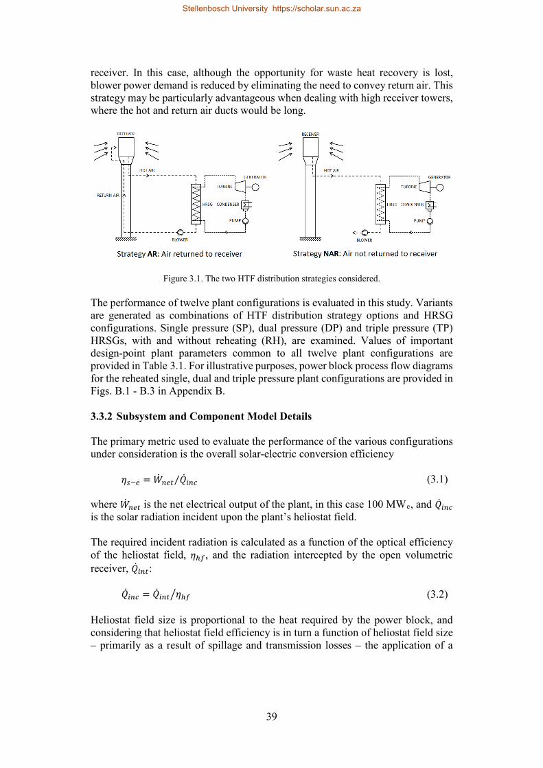
39

receiver. In this case, although the opportunity for waste heat recovery is lost, blower power demand is reduced by eliminating the need to convey return air. This strategy may be particularly advantageous when dealing with high receiver towers, where the hot and return air ducts would be long.

Figure 3.1. The two HTF distribution strategies considered. The performance of twelve plant configurations is evaluated in this study. Variants are generated as combinations of HTF distribution strategy options and HRSG configurations. Single pressure (SP), dual pressure (DP) and triple pressure (TP) HRSGs, with and without reheating (RH), are examined. Values of important design-point plant parameters common to all twelve plant configurations are provided in Table 3.1. For illustrative purposes, power block process flow diagrams for the reheated single, dual and triple pressure plant configurations are provided in Figs. B.1 - B.3 in Appendix B. 3.3.2 Subsystem and Component Model Details The primary metric used to evaluate the performance of the various configurations under consideration is the overall solar-electric conversion efficiency 𝜂𝜂𝑠𝑠−𝑒𝑒 = ��𝑊𝑛𝑛𝑒𝑒𝑛𝑛 ��𝑄𝑖𝑖𝑛𝑛𝑖𝑖⁄ (3.1)

where ��𝑊𝑛𝑛𝑒𝑒𝑛𝑛 is the net electrical output of the plant, in this case 100 MWe, and ��𝑄𝑖𝑖𝑛𝑛𝑖𝑖 is the solar radiation incident upon the plant’s heliostat field. The required incident radiation is calculated as a function of the optical efficiency of the heliostat field, 𝜂𝜂ℎ𝑓𝑓, and the radiation intercepted by the open volumetric receiver, ��𝑄𝑖𝑖𝑛𝑛𝑛𝑛: ��𝑄𝑖𝑖𝑛𝑛𝑖𝑖 = ��𝑄𝑖𝑖𝑛𝑛𝑛𝑛 𝜂𝜂ℎ𝑓𝑓� (3.2)

Heliostat field size is proportional to the heat required by the power block, and considering that heliostat field efficiency is in turn a function of heliostat field size – primarily as a result of spillage and transmission losses – the application of a


40

constant heliostat field efficiency for all plant configurations introduces error. Dedicated modelling of heliostat field performance was considered beyond the scope of this work, however. Instead, a functional relationship between heliostat field efficiency and size was regressed from data presented by Avila-Marin and Tellez Sufrategui [127]. As part of their study, they employed the WinDelsol optical modelling code [128], based on the well-established Delsol program, to evaluate the design-point optical efficiencies of state-of-the-art, surround-type heliostat fields associated with molten salt central receiver CSP plants of various sizes. Although there are distinct differences between the molten salt and open volumetric receivers, they operate at similar levels of mean solar flux and fairly similar thermal efficiencies in practice. This in turn implies that for a given receiver thermal load, molten salt and open volumetric receivers will share approximately similar physical dimensions.

Table 3.1. Nominal design-point plant parameters common to all plant configurations.

Parameter Value Ambient Parameters Temperature [°C] 30 Pressure [bar] 1 Receiver Parameters Maximum mean solar flux [kW/m2] 500 Air return ratio [-] 0.5 HTF Distribution System Parameters Temperature drop: hot duct [K] 10 Temperature drop: return duct [K] 5 Blower isentropic efficiency [-] 0.6 HRSG Parameters Approach point temperature difference [K] 5 Pinch point temperature difference [K] 10 Water/Steam Cycle Parameters Steam turbine isentropic efficiency [-] 0.85 Live/RH steam temperature [°C] 560 Maximum live steam pressure [bar] 165 IP steam pressure [bar] 15 LP steam pressure [bar] 5 Air-cooled condenser initial temperature difference [K] 25 Minimum steam dryness at turbine outlet [-] 0.9 Deaerator outlet temperature [°C] 60

As such, the data presented by Avila-Marin and Tellez Sufrategui was deemed suitable for use in this study. In particular, heliostat field data calculated for three plants (50, 75 & 100 MWe) located at Daggett, California were used to regress a linear function predicting heliostat field efficiency as a function of the required receiver heat transfer rate, ��𝑄𝑟𝑟𝑒𝑒𝑖𝑖 (MW), given by Eq. (3.3). The regression is shown along with the published data in Fig. 3.2.


41

𝜂𝜂ℎ𝑓𝑓 = −8.17663 × 10−5 ��𝑄𝑟𝑟𝑒𝑒𝑖𝑖 + 0.700436 (3.3) The radiation that must be intercepted by the open volumetric receiver is dependent upon the required receiver heat transfer rate and the receiver thermal efficiency, 𝜂𝜂𝑟𝑟𝑒𝑒𝑖𝑖: ��𝑄𝑖𝑖𝑛𝑛𝑛𝑛 = ��𝑄𝑟𝑟𝑒𝑒𝑖𝑖 𝜂𝜂𝑟𝑟𝑒𝑒𝑖𝑖⁄ (3.4)

In general, OVR thermal efficiency is challenging to model accurately as it is primarily dependent upon fairly complex radiative and convective heat transfer mechanisms that take place both at the surface and within the receiver’s porous absorber. Instead of implementing a physical model of the OVR in this study, therefore, the thermodynamic behaviour of the receiver was captured by a quadratic regression of quasi-steady state test data associated with the 200 kWth “SolAir” OVR, as presented by Téllez [42]. In particular, the data used here was derived from the second absorber configuration considered in the test campaign, which comprised a combination of recrystalised SiC and SiSiC absorber modules. The latter SiSiC modules formed the basis for the modules employed in the Solar Tower Jülich OVR plant [8], and are thus representative of the state-of-the-art.

Figure 3.2. Design-point heliostat field efficiency and receiver tower height as functions of design-point receiver heat transfer rate fitted to data from Avila-Marin and Tellez Sufrategui [127].

Based on the SolAir test data, a second order relationship between receiver thermal efficiency and specific intercepted radiation, ��𝑄𝑖𝑖𝑛𝑛𝑛𝑛 ��𝑚𝑎𝑎⁄ , was established via regression analysis and is given by Eq. (3.5), which is plotted along with the test data in Fig. 3.3. The denominator, ��𝑚𝑎𝑎, is the mass flow rate of air passing through the receiver. In addition, the maximum mean solar flux was specified as 500 kW/m2 on the basis of the range of mean flux values associated with the SolAir test data. 𝜂𝜂𝑟𝑟𝑒𝑒𝑖𝑖 = −0.578629��𝑄𝑖𝑖𝑛𝑛𝑛𝑛 ��𝑚𝑎𝑎⁄ �2 + 0.741229��𝑄𝑖𝑖𝑛𝑛𝑛𝑛 ��𝑚𝑎𝑎⁄ � + 0.621714 (3.5)


42

The major assumption made by the receiver modelling approach outlined above is that the solar radiation intercepted by the OVR is uniformly distributed across its surface, which is not the case practically. It is nevertheless felt that such a simplification is reasonable considering the exploratory nature of this study. ��𝑄𝑟𝑟𝑒𝑒𝑖𝑖 can be represented in terms of the receiver air mass flow rate and the difference in the receiver outlet, ℎ𝑜𝑜, and inlet, ℎ𝑖𝑖, air enthalpies: ��𝑄𝑟𝑟𝑒𝑒𝑖𝑖 = ��𝑚𝑎𝑎(ℎ𝑜𝑜 − ℎ𝑖𝑖) (3.6)

To determine the enthalpy of the air at the receiver inlet, ℎ𝑖𝑖, when exhaust air from the HRSG is returned to the receiver, a mixing rule was used in accordance with Téllez [42]: ℎ𝑖𝑖 = (1 − 𝑅𝑅𝑟𝑟𝑒𝑒𝑛𝑛) ℎ𝑎𝑎𝑎𝑎𝑎𝑎 + 𝑅𝑅𝑟𝑟𝑒𝑒𝑛𝑛 ℎ𝑟𝑟𝑒𝑒𝑛𝑛 (3.7)

where 𝑅𝑅𝑟𝑟𝑒𝑒𝑛𝑛 is the assigned air return ratio, ℎ𝑎𝑎𝑎𝑎𝑎𝑎 is the ambient air enthalpy and ℎ𝑟𝑟𝑒𝑒𝑛𝑛 is the enthalpy of the air being returned to the receiver. The nominal air return ratio considered in this study was 0.5; a value that has been demonstrated to be achievable [32].

Figure 3.3. Receiver thermal efficiency as a function of specific intercepted radiation fitted to SolAir experimental data from Téllez [42].

To evaluate the pressure drop through the receiver’s porous absorber, Δ𝑝𝑝𝑟𝑟𝑒𝑒𝑖𝑖, a discrete approximation of the Forchheimer-Darcy equation is used:

Δ𝑝𝑝𝑟𝑟𝑒𝑒𝑖𝑖 = 𝐿𝐿 �𝜇𝜇𝑎𝑎|𝑇𝑇𝑜𝑜 ��𝑚𝑎𝑎

𝑘𝑘1 𝜌𝜌𝑎𝑎|𝑇𝑇𝑜𝑜,𝑝𝑝𝑎𝑎𝑎𝑎𝑎𝑎 𝐴𝐴𝑟𝑟𝑒𝑒𝑖𝑖+

��𝑚𝑎𝑎2

𝑘𝑘2 𝜌𝜌𝑎𝑎|𝑇𝑇𝑜𝑜,𝑝𝑝𝑎𝑎𝑎𝑎𝑎𝑎 𝐴𝐴𝑟𝑟𝑒𝑒𝑖𝑖2 � (3.8)

Here, 𝐿𝐿 is the absorber thickness (0.1 m), 𝜇𝜇𝑎𝑎 is the dynamic viscosity of air evaluated at the receiver outlet temperature, 𝜌𝜌𝑎𝑎 is the density of air evaluated at the receiver


43

outlet temperature and ambient pressure, and 𝐴𝐴𝑟𝑟𝑒𝑒𝑖𝑖 is the receiver frontal surface area. The parameter 𝑘𝑘1 is the permeability coefficient which represents the permeability of the porous absorber medium, while 𝑘𝑘2 is the inertial coefficient which invokes the nonlinear contribution to pressure loss of inertial effects associated with high flow velocity. Values for these latter two parameters were obtained from Becker et al. [31] as 10-7 m2 and 0.011 m, respectively, which are consistent with the absorber material considered here. The HTF distribution system model comprises the duct and blower component models. The duct model characterises the drop in pressure and temperature experienced by the air, as it flows within the supply and return ducts. In the air return (AR) scenario, the supply and return duct lengths were each estimated to be the sum of the receiver tower height, ℎ𝑛𝑛𝑜𝑜𝑡𝑡, and an additional 20 m of ducting to reach the HRSG, which was assumed to be stationed at ground level. In addition, each duct incorporated three vaned mitre bends, and within the tower the supply and return ducts were assumed to be positioned parallel to each other. In the no air return (NAR) scenario, the supply duct incorporated just one vaned mitre bend and its length was determined to be the sum of ℎ𝑛𝑛𝑜𝑜𝑡𝑡 and an additional 10 m of ducting. Receiver tower height was assumed to vary primarily as a function of the required receiver heat transfer rate, ��𝑄𝑟𝑟𝑒𝑒𝑖𝑖. The function employed in this work was linearly regressed from data presented in the study by Avila-Marin and Tellez Sufrategui, as described above. The resulting dependency of ℎ𝑛𝑛𝑜𝑜𝑡𝑡 (m) on ��𝑄𝑟𝑟𝑒𝑒𝑖𝑖 is expressed in Eq. (3.9) and shown graphically in Fig. 3.3. ℎ𝑛𝑛𝑜𝑜𝑡𝑡 = 1.99622 × 10−1 ��𝑄𝑟𝑟𝑒𝑒𝑖𝑖 + 97.1461 (3.9)

All duct wetted surfaces were assigned a surface roughness of 0.015 mm, which is consistent with that of galvanised steel [129]. The Colebrook equation was used to determine the friction factors, 𝑓𝑓𝑑𝑑𝑑𝑑𝑖𝑖, associated with each duct under the prevailing flow conditions, allowing an evaluation of the associated pressure drops according to ∆𝑝𝑝 = (𝑓𝑓𝑑𝑑𝑑𝑑𝑖𝑖(𝐿𝐿𝑑𝑑𝑑𝑑𝑖𝑖 𝐷𝐷𝑑𝑑𝑑𝑑𝑖𝑖⁄ ) + 𝑛𝑛𝑎𝑎𝑒𝑒𝑛𝑛 𝑘𝑘𝑎𝑎𝑒𝑒𝑛𝑛)�𝜌𝜌𝑎𝑎𝑖𝑖𝑟𝑟 𝑣𝑣𝑑𝑑𝑑𝑑𝑖𝑖2 2⁄ � (3.10)

where 𝐿𝐿𝑑𝑑𝑑𝑑𝑖𝑖 and 𝐷𝐷𝑑𝑑𝑑𝑑𝑖𝑖 represent duct length and diameter, respectively, 𝑛𝑛𝑎𝑎𝑒𝑒𝑛𝑛 and 𝑘𝑘𝑎𝑎𝑒𝑒𝑛𝑛 denote the number of mitre bends and the mitre bend loss coefficient, respectively, 𝜌𝜌𝑎𝑎𝑖𝑖𝑟𝑟 represents the mean air density within the duct, and 𝑣𝑣𝑑𝑑𝑑𝑑𝑖𝑖 is the mean duct velocity, nominally assigned to be 30 m/s. For this study, the mitre bend loss coefficient was taken to be 0.25 [129]. The mean duct velocity specification enabled the determination of the supply and/or return duct diameters on the basis of the required air mass flow rate. Duct temperature drops were treated as constant in all simulations, with values of -10 K and -5 K assigned to the supply and return ducts, respectively.


44

The blower model is employed to determine the blower outlet temperature and power consumption associated with the required air mass flow rate, pressure ratio, and the given blower isentropic efficiency, which is treated as constant. The heat recovery steam generator subsystem model comprises component models to account for steady-state heat exchange between the air and water/steam streams in applicable economisers, evaporators, superheaters and reheaters. The reference values for the approach point temperature difference ∆𝑁𝑁𝑎𝑎𝑝𝑝, and the pinch point temperature difference ∆𝑁𝑁𝑝𝑝𝑝𝑝, were taken as 5 K and 10 K, respectively. These values are in line with those presented by Kehlhofer et al. [124]. For the sake of clarity, ∆𝑁𝑁𝑎𝑎𝑝𝑝 is defined as being the difference between the water-side economiser outlet temperature and evaporator saturation temperature, whilst ∆𝑁𝑁𝑝𝑝𝑝𝑝 is the difference between the evaporator saturation temperature and the gas-side evaporator outlet temperature. Pressure loss fractions in applicable economisers, superheaters and reheaters are prescribed based on values in Kehlhofer et al., and blowdown loss fractions associated with applicable evaporators are obtained from Ganapathy [130]. Furthermore, it was assumed that 1% of the heat conveyed in the air stream is lost as a result of imperfect HRSG insulation. This value is within the range typical of HRSGs [130]. In accordance with Kehlhofer et al., the log mean temperature difference method is used to evaluate the product of overall heat transfer coefficient and surface area. In all configurations considered, a deaerator is used to provide slight feedwater heating to 60 °C. This is the value typically associated with combined cycle plants burning natural gas, which is high enough to prevent acidic condensation on the gas-side heat exchanger surfaces [124]. During solar-only operation of OVR CSP plants, the gas-side stream doesn’t contain combustion products and thus a lower feedwater temperature could be tolerated. However, to accommodate for the possibility of hybridised operation, a temperature of 60 °C is employed. All steam turbines are modelled as single-stage expanders with isentropic efficiencies of 0.85. In cases involving multi-pressure configurations, only partial superheating is applied to the intermediate pressure (IP) loops to ensure sufficient loop mass flow rate. That is, superheating is undertaken to a temperature below that corresponding to the intersection point of the IP loop isobar and the turbine expansion line. Furthermore, superheating is not applied in the low pressure (LP) loops. The inlet conditions to the intermediate and low pressure turbines are therefore determined using simple mixing rules. For this study, live and reheat steam temperatures are set to 560 °C, whilst the maximum allowable live steam pressure is restricted to 165 bar. These values are within the steam parameter ranges typically associated with steam turbines appropriate for CSP operation, as outlined, for example, in [131]. For all multi-pressure configurations, the LP pressure is set to 5 bar in accordance with recommendations by Kehlhofer et al., whilst for the triple pressure configurations, an IP pressure of 15 bar is applied, as this is shown


45

by simulations to yield approximately the best overall plant performance for the variation of independent variables considered. The air-cooled condenser (ACC) model incorporates fixed initial and terminal temperature differences of 25 K and 10 K relative to the dry-bulb ambient temperature, respectively. These values are typical of contemporary ACCs. The ACC model also accounts for a fixed water/steam-side pressure drop and the fan power required to overcome the air-side pressure drop is included as a parasitic loss. All water pumps are modelled according to a constant isentropic efficiency of 80 %, whilst the blower is specified to have an isentropic efficiency of 60 %; a value typical of blowers of the scale considered here [129]. The motors for pumps, ACC fans and the blower are assumed to have an electrical efficiency of 0.96. The plant’s electrical generator is assigned an electrical efficiency of 0.98. 3.3.3 Model Validation To assess the validity of the HTF distribution system and power block modelling methodology, the performance predicted for a single pressure plant with air return but without reheat was compared to predictions made by Eck et al. [53] for a similar plant. To predict the design-point performance of the reference plant, Eck et al. employed the IPSEpro simulation software. Several design-point inputs that could be deduced from the data provided in the reference work were used to align the validation plant parameters to those of the reference plant. These included a net electrical power output of 100 MW, live steam parameters of 550 °C and 110 bar, a condenser temperature of 54 °C, a heliostat field efficiency of 66.2 %, and a receiver thermal efficiency of 70.3 %. All other required inputs that could not be deduced were estimated within reasonable limits. Comparative results are provided in Table 3.2.

Table 3.2. Comparison of predicted and reference plant performance indices.

Performance Index Reference Value

Predicted Value

Deviation

Net power output [MWe] 100 100 - Heliostat field optical efficiency [%] 66.2 66.2 - Receiver thermal efficiency [%] 70.3 70.3 - Receiver air mass flow rate [kg/s] 467.2 464.2 -0.6 % Live steam mass flow rate [kg/s] 97.6 95.0 -2.7 % Parasitic power demand [MWe] 9.7 9.5 -2.0 % Gross water/steam cycle thermal efficiencya [%] 34.6 34.9 +0.9 % Solar-electric efficiency [%] 14.7 14.8 +0.7 %

Note: aDefined as the ratio of gross electrical power to HRSG heat transfer rate. The deviations shown in Table 3.2 indicate very good agreement between the predicted and references performance indices, with all deviations being beneath 3%. Given the uncertainty associated with a number of important reference plant


46

parameters, the authors believe that this level of agreement indicates the suitability of the methodology employed to model the combined HTF distribution system and power block. 3.4 Results and Discussion 3.4.1 Impact of Receiver Outlet Temperature Figure 3.4 illustrates the trends in solar-electric efficiency for all air return (AR) configurations as a function of receiver outlet temperature.

Figure 3.4. Influence of solar-electric efficiency over a range of varying receiver outlet temperature for all air return configurations.

It can be observed that maximum and minimum receiver outlet temperatures applicable to each configuration vary. At the lower end of the range, a limit exists as a consequence of superheater inlet temperature difference restrictions, whilst at the higher end, limitations are imposed either by economiser outlet temperature difference restrictions or in instances where the low pressure steam mass flow rate falls beneath a practical limit of 1 kg/s. Nonetheless, significant differences in configuration performances are evident. At low receiver outlet temperatures, approximately equivalent to inlet temperatures associated with unfired combined cycle HRSGs, the multi-pressure cycles offer the highest performance, with reheating significantly improving solar-electric efficiency. As the receiver outlet temperature increases, the solar-electric efficiency of all configurations improves. This behaviour indicates that gains in HRSG exergy utilisation supersede the increased receiver losses incurred. Also noteworthy is that the greatest performance gains are made by the SP configurations whose receiver outlet temperatures are not as restricted by the mass flow rate limitations encountered by the multi-pressure cycles. These gains, however, are achieved from


47

lower starting values and are ultimately limited by HRSG outlet temperature difference restrictions. As a result, the DP&RH configuration is shown to exhibit the best plant performance, with a maximum solar-electric efficiency of 17.4 %. The next best performing configuration is the significantly more complex TP&RH plant with a peak efficiency of 17.3 %, followed by the reheated single pressure configuration having a peak efficiency of 16.9 %. The best performing configuration without reheat is predicted to be the triple pressure plant with a reduced efficiency of 15.9 %. It is also interesting to note that the single pressure configuration outperforms the dual pressure configuration at peak values. In the context of the above results, it is important to note that in conventional combined cycle power plants, triple pressure configurations prove optimal when the HRSG receives heat directly from the upstream gas turbine, whilst single pressure configurations offer the best performance when the gas turbine exhaust is supplementary fired. Overall combined cycle performance in non-supplementary fired plants is best at lower gas turbine exhaust temperatures, as gas turbine efficiency is improved. When supplemental firing is employed, higher HRSG inlet temperatures enable the power output of the water/steam cycle to be boosted. In this scenario, a single pressure configuration typically offers the best HRSG exergetic efficiency. In OVR CSP plants, the absolute limit of the receiver outlet temperature, and thus the HRSG inlet temperature, is set by the maximum permissible absorber material temperature. Furthermore, the peak permissible temperatures of contemporary ceramic absorber materials are well in excess of conventional combined cycle HRSG inlet temperatures. In itself, this may suggest that the single pressure configuration would offer the best design-point performance. The results reflected in Fig. 3.4, however, indicate that for the configurations examined here, this is clearly not found to be the case. This is a significant observation; one which arises from the thermodynamic coupling that exists between the OVR and the HRSG, manifesting primarily as a result of the concurrence of falling receiver efficiency and rising HRSG heat recovery as receiver outlet temperature is increased. The water/steam cycle temperature-entropy diagrams and the HRSG temperature-cumulative heat transfer rate diagrams associated with the best performing SP&RH, DP&RH and TP&RH air return configurations are shown in Figs. 3.5 - 3.10. The 𝑁𝑁 − 𝑠𝑠 diagrams indicate the impact that reheating has on live steam pressure and illustrate the manner in which the low and intermediate pressure loops are incorporated into the multi-pressure plants. Although the degree of reheating is shown to be relatively low, the solar-electric efficiency results clearly indicate its importance with respect to plant performance enhancement, which is an important finding. Observation of the 𝑁𝑁 − ��𝑄 diagrams provides insight into the exergy utilisation characteristics of each HRSG. The high inlet temperature of the SP&RH HRSG enables a matching of the heat capacitance rates of the air and water/steam streams in the economiser, suggesting excellent exergy utilisation here. However,


48

a greater HRSG inlet temperature difference offsets this benefit somewhat, leading to a total required heat transfer rate of 306.2 MW. In the DP&RH configuration, with a total required heat transfer rate of 301.2 MW, the inlet temperature difference is reduced, enabling better overall exergy utilisation despite the fact that evaporation of the low pressure steam reduces heat capacitance rate compatibility in the high and low pressure economisers. The TP&RH configuration, with a total required heat transfer rate of 307.2 MW, enables an even lower inlet temperature difference, but the combination of the low and intermediate pressure evaporators restricts heat capacitance rate matching beyond the high pressure evaporator.

Figure 3.5. Temperature-entropy diagram for the SP&RH air return configuration at peak performance.

Figure 3.6. HRSG temperature-cumulative heat transfer rate diagram for the SP&RH air return configuration at peak performance.


49

Figure 3.7. Temperature-entropy diagram for the DP&RH air return configuration at peak performance.

Figure 3.8. HRSG temperature-cumulative heat transfer rate diagram for the DP&RH air return configuration at peak performance.

Table 3.3 highlights noteworthy heat and work transfer rates associated with the six air return plant configurations for the receiver outlet temperature permitting best design-point performance. Also indicated are associated values for heliostat field optical efficiency, receiver thermal efficiency, net power block thermo-electric efficiency, 𝜂𝜂𝑝𝑝𝑎𝑎, and plant solar-electric efficiency. In interpreting Table 3.3, it is important to note that each configuration is subjected to an assumed auxiliary parasitic power demand of 2.5 MW, which is not reflected in the table.


50

Figure 3.9. Temperature-entropy diagram for the TP&RH air return configuration at peak performance.

Figure 3.10. HRSG temperature-cumulative heat transfer rate diagram for the TP&RH air return configuration at peak performance.

The data Table 3.3 reflects enable illustrative comparisons to be drawn between each configuration and an evaluation of how associated HRSG characteristics impact upon component sizing. For instance, the required incident solar radiation, ��𝑄𝑖𝑖𝑛𝑛𝑖𝑖, is directly proportional to heliostat field size. It is clear to see that in this regard, the data imply that there is a significant variation in field size between configurations. The best-performing DP&RH configuration would, in theory, have a field size 6.1 % smaller than the conventionally-proposed SP configuration, and 8.4 % smaller than the worst-performing TP configuration. Assuming an equivalent mean solar flux imposed upon the receiver of each configuration, the required intercepted radiation, ��𝑄𝑖𝑖𝑛𝑛𝑛𝑛, data suggest that the DP&RH configuration would require a receiver 5.8 % smaller in surface area than that of the SP configuration,


51

and 8.0 % smaller than that of the TP configuration. Similar implications regarding component size can be deduced from the data presented for the rate of heat rejection in the air-cooled condenser, ��𝑄𝑎𝑎𝑖𝑖𝑖𝑖. The rate of transfer within the HRSG is denoted as ��𝑄𝐻𝐻𝐻𝐻𝐻𝐻𝐻𝐻.

Table 3.3. Heat and work transfer rates, as well as efficiencies associated with the six air return plant configurations.

Configuration SP SP&RH DP DP&RH TP TP&RH Heat transfer rates [MWth] ��𝑄𝑖𝑖𝑛𝑛𝑖𝑖 611.4 591.0 611.7 574.4 627.3 579.2 ��𝑄𝑖𝑖𝑛𝑛𝑛𝑛 407.9 394.9 408.1 384.3 417.9 387.3 ��𝑄𝑟𝑟𝑒𝑒𝑖𝑖 334.8 326.8 342.0 322.2 356.6 328.8 ��𝑄𝐻𝐻𝐻𝐻𝐻𝐻𝐻𝐻 316.9 308.5 320.4 301.2 330.9 307.2 ��𝑄𝑎𝑎𝑖𝑖𝑖𝑖 202.9 194.0 204.2 184.8 206.8 184.2 Work transfer rates [MW] ��𝑊𝑛𝑛 109.8 110.1 109.9 110.2 110.2 110.2 ��𝑊𝑎𝑎𝑏𝑏𝑜𝑜 2.4 2.4 2.6 2.5 3.0 2.6 ��𝑊𝑓𝑓𝑎𝑎𝑛𝑛 3.2 3.1 3.3 2.9 3.3 2.9 ��𝑊𝑝𝑝𝑑𝑑𝑎𝑎 1.7 2.1 1.5 2.3 1.4 2.2 Efficiencies [%] 𝜂𝜂ℎ𝑓𝑓 66.7 66.8 66.7 66.9 66.6 66.9

𝜂𝜂𝑟𝑟𝑒𝑒𝑖𝑖 82.1 82.8 83.8 83.9 85.3 84.9 𝜂𝜂𝑝𝑝𝑎𝑎 31.6 32.4 31.2 33.2 30.2 32.6

𝜂𝜂𝑠𝑠−𝑒𝑒 16.5 16.9 16.4 17.4 15.9 17.3

It is interesting to note that values predicted for shaft power yielded by the steam turbine/s associated with each plant configuration, ��𝑊𝑛𝑛, lie within a fairly narrow band. The resulting implication of this is that in a cumulative sense, total parasitic power demand is roughly equivalent across plant configurations, despite the significant variations in the size of key non-power block components indicated by the heat transfer rate data. Furthermore, despite not being the best-performing configuration overall, the SP&RH configuration would require a slightly smaller steam turbine than that of the DP&RH plant. Greater variation in component sizing is implied by the shaft power demands predicted for the blower, ��𝑊𝑎𝑎𝑏𝑏𝑜𝑜, the air-cooled condenser fans, ��𝑊𝑓𝑓𝑎𝑎𝑛𝑛, and the feedwater pumps, ��𝑊𝑝𝑝𝑑𝑑𝑎𝑎. In regards to blower power consumption, it is noteworthy that the SP and SP&RH configurations incur slightly lower blower losses than the best-performing DP&RH configuration. This can be explained by the fact that since the receiver outlet temperatures reached by the SP and SP&RH configurations are higher than those reached by the DP&RH configuration, a lower HTF mass flow rate is required by the receiver to provide sufficient heat to the HRSG, and thus the blower power demand is reduced. This is confirmed by the results reflected in Fig. 3.11, which


52

presents receiver air mass flow rates of the AR configurations as a function of receiver outlet temperature.

Figure 3.11. Receiver air mass flow rate vs. receiver outlet temperature for all air return configurations.

Most striking is the degree to which an increase in receiver outlet temperature reduces the required air mass flow rate through the OVR for all configurations. For instance, for the SP configurations, the reduction is of the order of almost 50 %. At peak performance, the lowest mass flow rate is predicted for the SP&RH plant (451.8 kg/s), whilst the highest is predicted for the TP plant (564.4 kg/s). From the point of view of capital and operational expenditure, the minimisation of the HTF mass flow rate is imperative, since it minimises the size and cost of the receiver, ducting and HTF blower, in addition to reducing parasitic power consumption. With regards to the blower power demand, Fig. 3.12 shows the relationship between the blower power fraction, which represents the blower power required as a percentage of the net plant power output of 100 MW, and the receiver outlet temperature for the AR configurations. These results correlate directly with the mass flow rate characteristics, since blower power is proportional to the HTF mass flow rate. Consequently, a significant reduction in blower power consumption in response to the elevation of receiver outlet temperature can be observed, with the lowest value of 2.4 % again being associated with the SP&RH plant for the reference conditions. Nonetheless, a parasitic loss of this magnitude illustrates a significant weakness of the OVR CSP plant concept, which is attributable to the inferior performance of atmospheric air as a heat transfer medium. To gauge the HRSG cost implications associated with each configuration, it is useful to compare the product of total heat transfer coefficient and area, 𝑁𝑁𝐴𝐴𝑛𝑛𝑜𝑜𝑛𝑛, calculated for each HRSG. Such a comparison is provided in Fig. 3.13, which displays 𝑁𝑁𝐴𝐴𝑛𝑛𝑜𝑜𝑛𝑛 values for the AR cases as functions of receiver outlet temperature.


53

Figure 3.12. Blower power fraction vs. receiver outlet temperature for all air return configurations. Moderate receiver outlet temperatures result in the lowest 𝑁𝑁𝐴𝐴𝑛𝑛𝑜𝑜𝑛𝑛 values for all configurations, above which values increase until the maximum permissible receiver outlet temperatures are reached. It can also be seen that the addition of reheating raises the 𝑁𝑁𝐴𝐴𝑛𝑛𝑜𝑜𝑛𝑛 required, appreciably at values of 𝑁𝑁𝑟𝑟𝑒𝑒𝑖𝑖,𝑜𝑜 where plant performance is highest, and significantly for the case of the reheated triple pressure cycle. At peak performance, the SP configuration is predicted to require the lowest 𝑁𝑁𝐴𝐴𝑛𝑛𝑜𝑜𝑛𝑛 value, whilst the highest value is predicted to be required by the TP&RH configuration. The distinctive “horseshoe” dependence of 𝑁𝑁𝐴𝐴𝑛𝑛𝑜𝑜𝑛𝑛 on 𝑁𝑁𝑟𝑟𝑒𝑒𝑖𝑖,𝑜𝑜 arises from the variance in the correlation between air and water/steam heat capacitance rates as the receiver outlet temperature is varied whilst the live steam parameters are held constant.

Figure 3.13. Total heat transfer coefficient – area product vs. receiver outlet temperature for all air return configurations.


54

Although the results shown in Fig. 3.13 indicate that reheated cycles will generally demand an increased heat transfer surface area, it is unlikely that the associated HRSG cost increase would be offset by the resulting solar field and receiver cost savings, given the significant improvement in solar-electric efficiency brought about by reheating. 3.4.2 Impact of Air Return Strategy When ground-stationed HRSGs are utilised in combination with high receiver towers, supply and return duct lengths become significant, giving rise to increased HTF blower power consumption to overcome comparatively high duct pressure drops. Under these conditions, pressure drop losses can be reduced by electing to exhaust the waste heat emanating from the HRSG to atmosphere, rather than returning it to the OVR, thereby mitigating the need for the return duct. The compromise that results from the no air return strategy, however, is that OVR inlet enthalpy is reduced, which in turn raises the required quantity of radiation intercepted by the OVR for a constant HTF mass flow rate. In this context, the impact of air return strategy on plant performance was studied by comparing results associated with the air return (AR) and non-air return (NAR) plant configurations simulated under reference conditions. Comparisons are drawn between the peak performing AR and NAR configurations for solar-electric efficiency and receiver air mass flow rate in Figs. 3.14 and 3.15, and for blower power fraction and the overall heat transfer coefficient – area product in Figs. 3.16 and 3.17.

Figure 3.14. Comparison of solar-electric efficiencies for all plant configurations at maximum receiver outlet temperature.

The predictions for peak solar-electric efficiency indicate a strong sensitivity to air return strategy, and for all plant configurations, the AR strategy is shown to result in distinctly higher efficiencies. This clearly implies that the reduction in blower


55

power demand associated with the NAR strategy is less significant than the impact of the thermal losses incurred as a result of waste heat rejection. Having said this, the NAR strategy consistently gives rise to lower HTF mass flow rates than those associated with the AR strategy, as illustrated in Fig. 3.15.

Figure 3.15. Comparison of receiver air mass flow rates for all plant configurations at maximum receiver outlet temperature.

Figure 3.16. Comparison of blower power fractions for all plant configurations at maximum receiver outlet temperature.

An explanation for this observation is provided by the blower power fraction predictions presented in Fig. 3.16. In all cases, the NAR strategy is shown to result in a substantially reduced blower power fraction, and in turn, a reduced parasitic power consumption. For a fixed net plant power output, reduced parasitic power demand decreases the gross power output required in addition to the rate at which


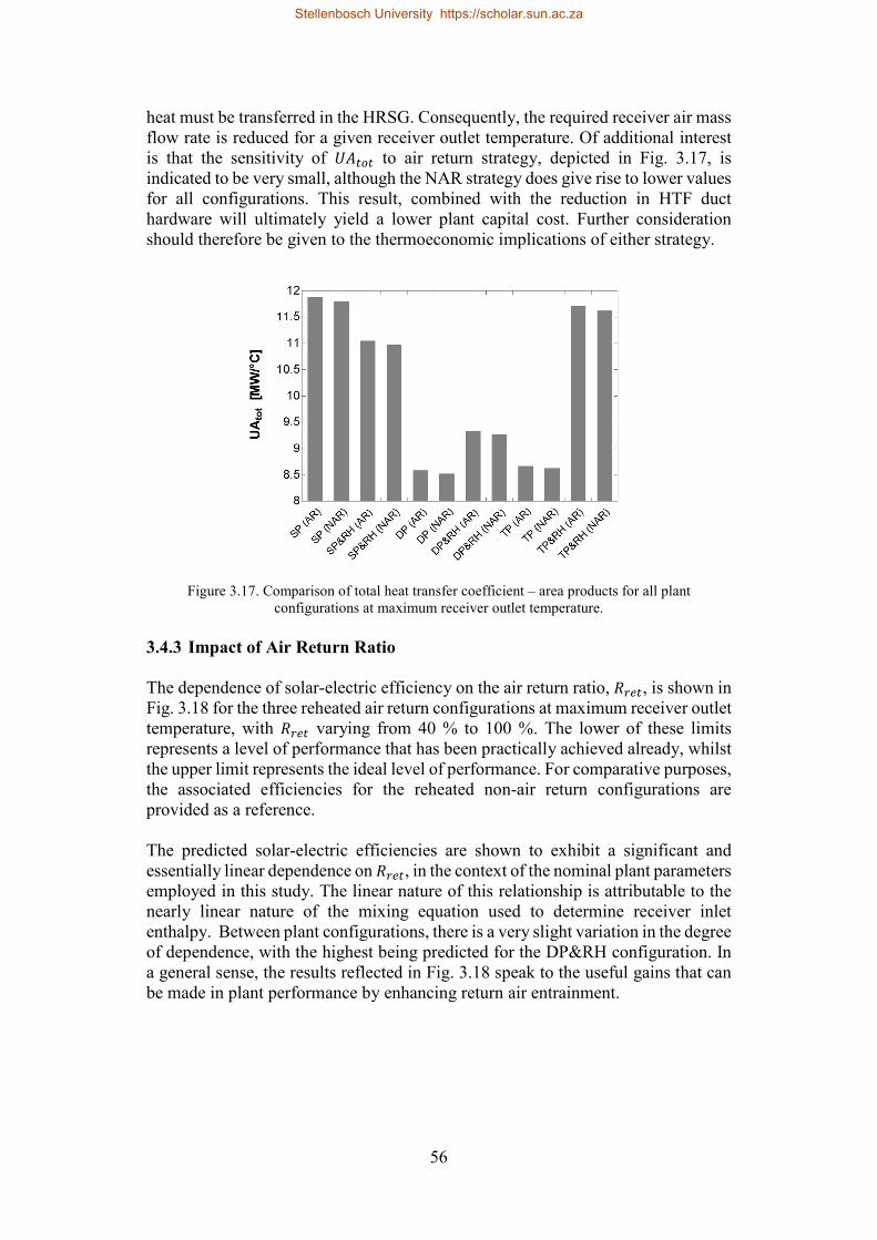
56

heat must be transferred in the HRSG. Consequently, the required receiver air mass flow rate is reduced for a given receiver outlet temperature. Of additional interest is that the sensitivity of 𝑁𝑁𝐴𝐴𝑛𝑛𝑜𝑜𝑛𝑛 to air return strategy, depicted in Fig. 3.17, is indicated to be very small, although the NAR strategy does give rise to lower values for all configurations. This result, combined with the reduction in HTF duct hardware will ultimately yield a lower plant capital cost. Further consideration should therefore be given to the thermoeconomic implications of either strategy.

Figure 3.17. Comparison of total heat transfer coefficient – area products for all plant configurations at maximum receiver outlet temperature.

3.4.3 Impact of Air Return Ratio The dependence of solar-electric efficiency on the air return ratio, 𝑅𝑅𝑟𝑟𝑒𝑒𝑛𝑛, is shown in Fig. 3.18 for the three reheated air return configurations at maximum receiver outlet temperature, with 𝑅𝑅𝑟𝑟𝑒𝑒𝑛𝑛 varying from 40 % to 100 %. The lower of these limits represents a level of performance that has been practically achieved already, whilst the upper limit represents the ideal level of performance. For comparative purposes, the associated efficiencies for the reheated non-air return configurations are provided as a reference. The predicted solar-electric efficiencies are shown to exhibit a significant and essentially linear dependence on 𝑅𝑅𝑟𝑟𝑒𝑒𝑛𝑛, in the context of the nominal plant parameters employed in this study. The linear nature of this relationship is attributable to the nearly linear nature of the mixing equation used to determine receiver inlet enthalpy. Between plant configurations, there is a very slight variation in the degree of dependence, with the highest being predicted for the DP&RH configuration. In a general sense, the results reflected in Fig. 3.18 speak to the useful gains that can be made in plant performance by enhancing return air entrainment.


57

Figure 3.18. Solar-electric efficiency vs. air return ratio for all reheated air return plant configurations at maximum receiver outlet temperature.

3.4.4 Impact of Pinch Point Temperature Difference Fig. 3.19 illustrates the sensitivity of the solar-electric efficiency and total heat transfer coefficient – area product parameters for all reheated air return plant configurations to changes in the HRSG pinch-point temperature difference, Δ𝑁𝑁𝑝𝑝𝑝𝑝. It can be observed that the efficiency predictions display a fairly weak sensitivity to Δ𝑁𝑁𝑝𝑝𝑝𝑝, even for a substantial variation in this parameter. For instance, the solar-electric efficiency of the DP&RH plant falls from 17.5 % to only 17.3 % for a substantial 10 K change in Δ𝑁𝑁𝑝𝑝𝑝𝑝.

Figure 3.19. Solar-electric efficiency and total heat transfer coefficient – area product vs. pinch-point temperature difference for all reheated air return plant configurations at maximum receiver

outlet temperature.


58

The performance sensitivity exhibited in this scenario is significantly lower. For the best DP&RH (AR) plant, reduction in solar-electric efficiency as Δ𝑁𝑁𝑝𝑝𝑝𝑝 is raised from 10 K to 20 K is less than 2.5 %. The greatest performance reduction is experienced by the SP&RH (NAR) configuration, which shows a decrease in solar-electric efficiency of slightly greater than 3 %. Whilst these data show that plant performance is relatively insensitive to pinch-point temperature difference, the associated sensitivity of the 𝑁𝑁𝐴𝐴𝑛𝑛𝑜𝑜𝑛𝑛 parameter, providing an indication of HRSG cost, is significant. In the case of the DP&RH (AR) plant, the 𝑁𝑁𝐴𝐴𝑛𝑛𝑜𝑜𝑛𝑛 value falls by over 33 % as Δ𝑁𝑁𝑝𝑝𝑝𝑝 is raised from 10 K to 20 K. This observation may have important thermoeconomic implications, and clearly requires further investigation. 3.4.5 Impact of Deaerator Outlet Temperature As an additional study, the sensitivity of solar-electric efficiency to the variation of deaerator outlet temperature for all reheated air return plants was evaluated, with the results reflected in Fig. 3.20.

Figure 3.20. Solar-electric efficiency vs. deaerator outlet temperature for all reheated air return plant configurations at maximum receiver outlet temperature.

Optimal deaerator outlet temperatures are indicated for each of the configurations within the temperature range of 60 - 140 °C. Furthermore, an increase in solar-electric efficiency can be observed as the deaerator outlet temperature is raised from the nominal simulation value of 60 °C to the optimal values. This general characteristic can primarily be attributed to an improvement in water/steam cycle efficiency in addition to receiver efficiency as the degree of feedwater heating is raised towards optimal values. For instance, the DP&RH configuration experiences a 3.9 % increase in net cycle thermal efficiency and a 0.6 % increase in receiver thermal efficiency as the deaerator outlet temperature is raised from 60 °C to 100 °C. Comparatively speaking, the SP&RH configuration enjoys the most notable appreciation in solar-electric efficiency, with the TP&RH configuration


59

experiencing the smallest gain. The optimal conversion efficiency obtained by the DP&RH configuration is nonetheless the highest. 3.4.6 Impact of HTF Duct Velocity To evaluate the significance of the HTF duct velocity on plant performance and duct size, the solar-electric efficiencies and supply and return duct diameters associated with all reheated air return plant configurations at maximum receiver outlet temperature were calculated for design-point duct velocities ranging from 10 m/s to 50 m/s. Results are shown in Fig. 21. Over the velocity range considered, solar-electric efficiency exhibits a non-negligible dependency, decreasing in magnitude as duct velocity is increased as a consequence of the corresponding increase in HTF blower losses. The degradation in efficiency is quantitatively similar for all three plant configurations, with absolute reductions of between 2.2 % and 2.4 %. In terms of the supply and return air ducts, it interesting to note the close similarity in the supply and return duct diameters of all three plant configurations across the design-point velocity range of 10 m/s to 50 m/s. This result confirms that for the nominal duct velocity of 30 m/s, there is little difference in duct sizing between the three best-performing plants.

Figure 3.21. Solar-electric efficiency and supply and return duct diameters vs. duct velocity for all reheated air return plant configurations at maximum receiver outlet temperature.

The results reflected in Fig. 3.21 clearly imply that there exists a thermoeconomically-optimum design-point duct velocity for each plant configuration. This is since a slight sacrifice in solar-electric efficiency is demonstrated to yield a significant decrease in duct size, and consequently, a reduction in capital costs. Again, such determinations can only be made on the basis of a dedicated thermoeconomic investigation.


60

3.5 Conclusion The current study addresses the lack of published literature investigating how OVR CSP plant performance is affected by HRSG configuration and operating parameters. The work has presented the design-point performance characteristics of twelve plant configurations, distinguished by the number of water/steam cycle pressure levels and receiver air return strategy employed. A strong dependence of these characteristics on receiver outlet temperature was observed, illustrating the importance of accounting for thermodynamic coupling between subsystems in OVR CSP plant performance modelling. Within the bounds of technical constraints, best-performance operating points were determined for all configurations. The variation in peak solar-electric efficiency among the configurations considered is significant. Overall, the highest performance is exhibited by the air return reheated dual pressure plant. This result is contrary to what is shown to be the case in conventional combined cycle arrangements, where reheated triple pressure cycles typically offer optimum performance. Importantly, this finding is also contrary to the configurations considered in numerous prior works, including the studies by Romero et al. [30], Eck et al. [53] and Coelho et al. [109], [104], [23]. The reheated single and triple pressure plants with air return were shown to be almost as competitive as the reheated dual pressure plant. This result appears to indicate that from a thermoeconomic perspective, the simpler SP&RH configuration may be the most attractive of the air return configurations. As far as the return of waste heat from the HRSG to the receiver is concerned, results indicate that the air return strategy offers significant performance enhancements over the non-air return strategy at an air return ratio of 0.5. This is despite the added parasitic losses incurred by the plant as a result of increased blower power demand when air is returned to the receiver. Furthermore, a nearly linear relationship between solar-electric efficiency and air return ratio was observed, with the DP&RH showing marginally better performance gains as the air return ratio is increased in comparison to other configurations. In general, the results reinforced the importance of improving air return ratios in order to improve the competitiveness of OVR CSP plant technology. In regards to heat recovery steam generator performance, an increase of the pinch-point temperature difference parameter from 5 K to 15 K was shown to give rise to a significant reduction in overall solar-electric efficiency, whilst leading to only minor decreases in the product of overall heat transfer coefficient and heat exchange surface area. The air return SP&RH configuration displayed the highest sensitivity in regards to solar-electric efficiency, whilst the air return DP&RH exhibited the lowest. In addition, a notable sensitivity of solar-electric efficiency to deaerator outlet temperature was observed, with optimal efficiencies being indicated for all air return reheated plants. Finally, in as far as HTF duct velocity is concerned, simulation predictions indicated an appreciable sensitivity of solar-electric


61

efficiency and a very significant sensitivity of total duct diameter to variations in design-point duct velocity. From a thermodynamic perspective, the results presented in this paper have demonstrated distinct performance peaks associated with the various plant configurations considered, and suggest that the most efficient conversion of solar radiation into electricity is achieved by a dual pressure HRSG arrangement featuring reheat. However, questions exist as to whether certain performance enhancements can be made cost-effectively. It is therefore clear that a dedicated thermoeconomic analysis is required to determine which of the configurations would offer the lowest levelised cost of generation. Furthermore, the current study constituted a parametric analysis only in the context of design-point operation. Given that CSP plants generally operate away from the design-point, future work should give consideration to the impact of off-design operation on annualised performance of the best-performing configurations identified here.


62

4

Applicability of the Local Thermal Equilibrium Assumption in the Performance Modelling of CSP Plant Rock Bed Thermal Energy Storage Systems 4.1 Abstract Gas-solid packed beds have been widely studied as a cost-effective means of thermal energy storage in concentrating solar power (CSP) plants. Typically, the operation of packed beds in such systems is modelled by accounting for a finite rate of heat transfer between the fluid and solid media. This approach requires the coupled solution of the fluid- and solid-phase energy equations, which is computationally-costly, especially for year-long performance simulations. The local thermal equilibrium assumption, which assumes an infinite inter-phase heat transfer rate, can be applied to reduce the complexity and thus computational cost of packed bed models. However, the implications of making such an assumption in the context of CSP thermal energy storage system performance modelling is poorly understood. In fact, the application of the approach in long-term simulations has not been investigated before. This work addresses the topic by comparatively evaluating the performance of local thermal equilibrium and local thermal non-equilibrium models in the annual simulation of an air-rock packed bed, hypothetically operating in an open volumetric receiver CSP plant. The level of inter-model agreement is assessed in terms of annual bed exergy yield, bed blowing work, and plant power generation time. In addition, solution times are compared to establish the extent of computational cost savings. A parametric study examining the effect of variations in key bed design parameters on inter-model agreement is also conducted. The results obtained provide a clear indication of the strengths and weaknesses of either modelling approach, as well as of the suitability of the local thermal equilibrium assumption in general. 4.2 Introduction The use of packed beds with gaseous heat transfer fluids for sensible heat storage in concentrating solar power (CSP) plants has been widely considered for various forms of the technology. These include central receiver technologies such as open volumetric receiver (OVR) plants [68], fuel-hybridised OVR plants [109], solarised


63

gas turbine [132] and combined cycles [67], in addition to parabolic trough plants utilising air as a heat transfer fluid (HTF) [133]. The general operating principle of gas-solid packed bed TES systems is straightforward. During charging, hot gas is passed through the packed bed, convectively heating the solid medium and establishing a thermal gradient, or thermocline, within it. When the system is discharged, ambient air is passed through the bed in the reverse direction and is subsequently heated by the solid medium. The hot air leaving the bed is then passed through a heat exchanger to provide heat input to the plant’s power block. Figure 4.1 comparatively illustrates normalised thermoclines in the fluid and solid media of a typical packed bed at an instant in time. Thermocline shape is dependent upon a number of effects related to heat transfer and fluid flow within the bed. For packed bed models applied in CSP plant simulations, it is especially important that thermocline evolution is accurately predicted, since the calculation of overall plant performance is strongly sensitive to this characteristic.

Figure 4.1. Normalised fluid and solid thermoclines in a typical packed bed. This is as a consequence of a number of factors. The first is that the exergy contained by the bed is directly associated with thermocline shape. An acute thermocline indicates a higher exergy content than a more obtuse temperature profile. In turn, exergy content directly affects the energy yielded by the downstream power cycle, and thus overall plant performance. Secondly, since TES system operation is guided by the gas phase temperature at the bed outlet, excessively acute or obtuse thermoclines will give rise to premature or delayed activation or deactivation of the TES system. Deviations of this nature have a direct impact upon plant output. Thirdly, since the estimation of packed bed pressure drop relies on a knowledge of the bed’s gas phase temperature distribution, an unrealistic


64

thermocline will lead to an inaccurate evaluation of pressure losses. In turn, this will lead to an inaccurate estimate of parasitic losses and thus plant performance. As the rate at which heat is transferred between the HTF and storage medium is, in reality, finite, the gas and solid phases will not be in exact thermal equilibrium within the majority of a packed bed. Two-phase thermal performance models that account for this reality are therefore classified as Local Thermal Non-Equilibrium (LTNE) models. In various forms, LTNE models have been applied in the performance modelling of CSP-based gas-solid packed beds in numerous prior studies. Durisch et al. [134] applied an LTNE model to predict the performance of the proposed METAROZ plant [135]. The model was later enhanced and validated by Meier et al. [136]. Fricker [59] studied the operational characteristics of the TES system of the original PS10 plant design [96]. As part of a study on the thermo-mechanical behaviour of packed bed TES systems, Dreißigacker [69] applied an LTNE model to predict bed temperature distributions. Zunft et al. [68] went on to apply this model in a performance analysis of the TES system of the Solar Tower Jülich OVR plant [8]. Allen [61] employed the LTNE modelling approach to study the performance of rock bed TES systems, in the context of the SUNSPOT solarised combined cycle [64]. Hänchen et al. [74] applied an LTNE model to parametrically investigate the performance of a high temperature rock bed. In associated work, Zanganeh et al. [27] studied the performance of a large-scale TES system utilising the same technology. Zanganeh et al. [75] went on to use a similar modelling approach to design a rock bed TES system for use in an air HTF parabolic trough plant. Avila-Marin et al. [84] applied an LTNE model to simulate the behaviour of a high temperature laboratory-scale packed bed test facility. Heller [66] applied an LTNE model to design and analyse a pilot-scale TES system operating according to the SUNSPOT cycle. A concise summary of the study was later provided by Heller and Gauché [67]. The model was then used to investigate the performance of different solarised combined cycle configurations [113], a novel CSP plant concept employing a dual-pressure volumetric receiver – termed the SUNDISC cycle [54] – and later, to evaluate the thermoeconomic performance of the SUNDISC cycle [114]. Kuravi et al. [76] parametrically evaluated the performance of a packed bed featuring large-sized solid elements, Barton [78] formulated an LTNE model numerically solved using the finite volume method to study a rock bed TES system, and Mertens et al. [80] parametrically evaluated the performance of a rock bed integrated within an OVR CSP plant. As the implementation of LTNE models requires the coupled solution of the solid and fluid phase energy equations, annual performance simulations of CSP plants


65

featuring packed bed TES systems are computationally intensive. This can make parametric and optimisation studies cumbersome and potentailly impose limits on their scope. This consideration was acknowledged, for example, by Mertens et al. [80], who remarked that the LTNE model applied in their parametric study was implemented with reduced spatial resolution in order to limit computation time. Under certain thermal and fluid dynamic conditions, gas-solid packed beds can be modelled effectively using a simplified approach, where it is assumed that the rate of inter-phase heat transfer is sufficiently high that no appreciable inter-phase temperature difference exists [82]. This assumption gives rise to the Local Thermal Equilibrium (LTE) category of models that predict equivalent temperature distributions for both the solid and fluid phases, using just one energy equation. As a consequence of this simplification, the potential exists for the computational cost of long-term packed bed performance simulations to be significantly reduced, provided that the extent of the accompanying degradation in prediction fidelity is acceptable. LTE models are typically formulated in one of two ways. The simplest approach is to frame the energy equation as an advective type differential equation, where the passage of the thermal wave front is physically captured, but thermal dispersion effects are not. A more representative approach is to frame the energy equation as an advective-diffusive type differential equation, which incorporates an additional diffusion term to capture thermal dispersion. Of the relatively few CSP TES system modelling studies that have applied the LTE assumption, the majority have employed advective-diffusive LTE models. Avila-Marin et al. [85] applied such a model to parametrically study the performance of TES systems comprising various solid media. The agreement between predictions and test data was fair. Using the approach recommended by Kharchenko [71], Kronhardt et al. [70] employed an advective-diffusive LTE model to simulate the operation of the Solar Tower Jülich OVR plant TES system and compared the resulting predictions to measurements made at the facility. Simulated thermocline results exhibited fair agreement with measurement data. Anderson et al. [81] used a commercial CFD code to solve the advective-diffusive LTE problem associated with an alumina packed bed. In this latter study, simulation results demonstrated good agreement with experimental data. The limitations of the general LTE approach were also highlighted. In terms of advective type LTE modelling, the present authors have previously evaluated the suitability of the Infinite Number of Transfer Units (NTU) advective LTE model [82] in the long-term performance simulation of a CSP plant rock bed [13]. To this end, the performance of the Infinite NTU model was benchmarked against that of an associated the Effectiveness-NTU LTNE model. Despite its dramatically lower computational overhead, a critical short-coming of the Infinite NTU model was exhibited by its inability to accurately capture the diffusive evolution of the bed thermocline.


66

In the context of published literature, the computational efficiency and fidelity implications of applying the general LTE assumption in the annual performance modelling of gas-solid CSP TES systems have not been sufficiently established. Furthermore, the application of advective-diffusive LTE models in long-term simulations of such systems has not been specifically investigated. Considering the potential computational cost benefits that advective-diffusive type LTE models may present, this study seeks to comprehensively evaluate the applicability of this modelling approach. Specifically, the application of such a model to predict the annual performance characteristics of an above-ground, vertically-oriented, cylindrical rock bed CSP TES system is investigated. In this manner, the study serves as an extension of work previously undertaken [13], where the suitability of an advective type LTE model was evaluated. To facilitate the investigation, a rock bed TES system performance model incorporating an advective-diffusive LTE heat transfer model is formulated. The LTE model accounts for convective and radiative dispersion as well as thermal destratification during bed idle. Model validation is performed on the basis of relevant experimental data, and the model is then applied to simulate the performance of a utility-scale TES system operating over the course of a year. Model and simulation implementation was undertaken using the EES computational platform. Key performance predictions that result are benchmarked against those associated with an analogous LTNE model, the formulation of which is also detailed. In addition, comparisons are drawn between simulation solution times to evaluate the degree of computational cost benefit provided. 4.3 Model Formulation 4.3.1 One-Dimensional Energy Balances Assuming plug flow, no transverse heat transfer, no radiative heat transfer, no environmental heat loss, infinite thermal conduction within the solid phase, constant thermophysical properties, and that the solid phase can be represented by a continuous medium, the coupled fluid and solid phase energy balances associated with a packed bed can be written as:

𝜌𝜌𝑓𝑓 𝑐𝑐𝑝𝑝,𝑓𝑓 𝜖𝜖 𝜕𝜕𝑁𝑁𝑓𝑓𝜕𝜕𝑡𝑡

+ 𝐺𝐺𝑓𝑓 𝑐𝑐𝑝𝑝,𝑓𝑓 𝜕𝜕𝑁𝑁𝑓𝑓𝜕𝜕𝑧𝑧

= ℎ𝑣𝑣 �𝑁𝑁𝑠𝑠 − 𝑁𝑁𝑓𝑓� + 𝑘𝑘𝑓𝑓 𝜕𝜕2𝑁𝑁𝑓𝑓𝜕𝜕𝑧𝑧2

(4.1)

𝜌𝜌𝑠𝑠 𝑐𝑐𝑠𝑠 (1 − 𝜖𝜖) 𝜕𝜕𝑁𝑁𝑠𝑠𝜕𝜕𝑡𝑡

= ℎ𝑣𝑣 �𝑁𝑁𝑓𝑓 − 𝑁𝑁𝑠𝑠� + 𝑘𝑘𝑠𝑠 𝜕𝜕2𝑁𝑁𝑠𝑠𝜕𝜕𝑧𝑧2

(4.2)

Here, the fluid mass flux is defined as 𝐺𝐺𝑓𝑓 = ��𝑚𝑓𝑓 𝐴𝐴𝑎𝑎,𝑖𝑖⁄ . Equations (4.1) and (4.2) constitute the commonly-referred-to Continuous-Solid Phase model. For packed


67

beds where thermal conduction in both the fluid and solid phases can be ignored, the simpler, so-called Schumann model [137], then evolves:

𝜌𝜌𝑓𝑓 𝑐𝑐𝑝𝑝,𝑓𝑓 𝜖𝜖 𝜕𝜕𝑁𝑁𝑓𝑓𝜕𝜕𝑡𝑡

+ 𝐺𝐺𝑓𝑓 𝑐𝑐𝑝𝑝,𝑓𝑓 𝜕𝜕𝑁𝑁𝑓𝑓𝜕𝜕𝑧𝑧

= ℎ𝑣𝑣 �𝑁𝑁𝑠𝑠 − 𝑁𝑁𝑓𝑓� (4.3)

𝜌𝜌𝑠𝑠 𝑐𝑐𝑠𝑠 (1 − 𝜖𝜖) 𝜕𝜕𝑁𝑁𝑠𝑠𝜕𝜕𝑡𝑡

= ℎ𝑣𝑣 �𝑁𝑁𝑓𝑓 − 𝑁𝑁𝑠𝑠� (4.4)

If it is further assumed that the thermal capacity of the fluid phase is significantly less than that of the solid phase (as is the case in an air-rock system), the energy equations can be recast as:

𝜕𝜕𝑁𝑁𝑓𝑓𝜕𝜕𝑧𝑧

=𝐷𝐷𝑁𝑁𝑁𝑁𝐻𝐻𝑎𝑎

�𝑁𝑁𝑠𝑠 − 𝑁𝑁𝑓𝑓� (4.5)

𝜕𝜕𝑁𝑁𝑠𝑠𝜕𝜕𝑡𝑡

=𝐷𝐷𝑁𝑁𝑁𝑁𝜏𝜏

�𝑁𝑁𝑓𝑓 − 𝑁𝑁𝑠𝑠� (4.6)

The number of transfer units is defined as 𝐷𝐷𝑁𝑁𝑁𝑁 = ℎ𝑣𝑣 𝐻𝐻𝑎𝑎/(𝐺𝐺𝑓𝑓 𝑐𝑐𝑝𝑝,𝑓𝑓) and the thermal time constant is defined as 𝜏𝜏 = 𝜌𝜌𝑠𝑠 (1 − 𝜖𝜖) 𝐻𝐻𝑎𝑎 𝑐𝑐𝑠𝑠/(𝐺𝐺𝑓𝑓 𝑐𝑐𝑝𝑝,𝑓𝑓). Equations (4.5) and (4.6) were selected as the energy equations of the LTNE model considered here. The only thermal dispersion mechanism that they explicitly capture is that of inter-phase convection. At low bed Reynolds numbers, dispersion via bed conduction should generally be accounted for, as indicated by Summers et al. [138] and Adebiyi and Chenevert [139], who both recommended bed parameter thresholds above or below which bed conduction may be neglected. However, the findings of Hänchen et al. [74] and Zanganeh et al. [27] indicate that for conditions associated with air-rock CSP TES systems, the impact of bed conduction on performance predictions during charging or discharging is, in fact, negligible. With this said, bed conduction within an idle bed should not be neglected, as inter-phase convection is no longer dominant. In regards to radiative thermal dispersion, it is widely acknowledged that this effect becomes significant only at high bed temperatures, and where the bed fluid is gaseous [140]. In the literature, threshold temperature specifications vary fairly substantially from study to study, seemingly according to associated bed parameters. For instance, Balakrishnan and Pei [141] suggest a threshold of 250 °C, whereas Kunni and Smith [142] propose a value of 500 °C. In their study concerning an air-rock CSP TES system, Zanganeh et al. [27] investigated the impact of accounting for radiation on bed temperature profile. Allen [61] observed that with radiative dispersion neglected, their packed bed model over-predicted the


68

hot-end bed temperature by 15 – 25 °C after 8 hours of charging. This is a substantial deviation in consideration of power block sensitivity to peak HTF temperature. On the basis of these observations, it was concluded that the energy models formulated for the present study should account for radiative thermal dispersion when the bed is in operation. This is achieved by means of the widely-employed radiative “conductivity” approach. The formulation of the LTNE energy equations is based upon the Schumann model, which does not feature a conductive-type dispersion term in the solid-phase equation. However, as Vortmeyer and Schaefer [143] have demonstrated, if certain assumptions are made – consistent with the derivation of the LTNE and LTE models here – it can be shown that the single- and two-phase energy equations are “mathematically equivalent”. Based on this determination, Riaz [144] showed that by superposition, conductive-type thermal dispersion can be indirectly accounted for in the simplified Schumann model, by the definition of an “effective” volumetric heat transfer coefficient, ℎ𝑣𝑣,𝑒𝑒𝑓𝑓𝑓𝑓, quantified as 1 ℎ𝑣𝑣,𝑒𝑒𝑓𝑓𝑓𝑓⁄ = 1 ℎ𝑣𝑣,𝑖𝑖⁄ + 𝑘𝑘𝑎𝑎 �𝐺𝐺𝑓𝑓2 𝑐𝑐𝑝𝑝,𝑓𝑓

2 �⁄ (4.7) During charging and discharging, the bed conductivity term, 𝑘𝑘𝑎𝑎, is assumed here to incorporate only radiative dispersion, as quantified by the radiative conductivity of the bed, 𝑘𝑘𝑃𝑃𝑎𝑎𝑎𝑎. That is to say, 𝑘𝑘𝑎𝑎 = 𝑘𝑘𝑟𝑟𝑎𝑎𝑑𝑑. The term ℎ𝑣𝑣,𝑖𝑖 is the local volumetric heat transfer coefficient corrected according to the following correlation proposed by Jefferson [145], which relaxes the assumption of infinite intra-particle heat conduction: ℎ𝑣𝑣,𝑖𝑖 = ℎ𝑣𝑣 �1 + 𝐵𝐵𝐵𝐵𝑝𝑝 5⁄ �⁄ (4.8)

The term 𝐵𝐵𝐵𝐵𝑝𝑝 is the local particle Biot number defined as 𝐵𝐵𝐵𝐵𝑝𝑝 = ℎ 𝐷𝐷𝑝𝑝 2𝑘𝑘𝑠𝑠⁄ , where ℎ is the local heat transfer coefficient, defined as ℎ = 𝐷𝐷𝑁𝑁 𝑘𝑘𝑓𝑓 𝐷𝐷𝑝𝑝⁄ , and 𝐷𝐷𝑝𝑝 is the mean equivalent particle diameter. The volumetric heat transfer coefficient is related to ℎ by 𝑎𝑎, the particle surface area per unit volume of the bed, such that ℎ𝑣𝑣 = ℎ 𝑎𝑎. Approximating particle shape as spherical, 𝑎𝑎 = 6(1 − 𝜖𝜖) 𝐷𝐷𝑝𝑝⁄ . Consideration of an effective heat transfer coefficient results in the quantification of the number of transfer units changing to 𝐷𝐷𝑁𝑁𝑁𝑁 = ℎ𝑣𝑣,𝑒𝑒𝑓𝑓𝑓𝑓 𝐻𝐻𝑎𝑎/(𝐺𝐺𝑓𝑓 𝑐𝑐𝑝𝑝,𝑓𝑓). The correlations used to define the Nusselt number, 𝐷𝐷𝑁𝑁, and 𝑘𝑘𝑟𝑟𝑎𝑎𝑑𝑑 are provided in section 4.3.2. If the volumetric heat transfer coefficient in Eq. (4.1) and (4.2) is taken as being infinite, as is the basis of the local thermal equilibrium assumption, then the fluid and solid energy balances coalesce into a single equation that defines the variation of equivalent bed temperature associated with both phases:

�𝜌𝜌𝑓𝑓 𝑐𝑐𝑝𝑝,𝑓𝑓 + 𝜌𝜌𝑠𝑠 𝑐𝑐𝑠𝑠�𝜕𝜕𝑁𝑁𝑎𝑎𝜕𝜕𝑡𝑡

= 𝑘𝑘𝑎𝑎𝜕𝜕2𝑁𝑁𝑎𝑎𝜕𝜕𝑧𝑧2

− 𝐺𝐺𝑓𝑓 𝑐𝑐𝑝𝑝,𝑓𝑓𝜕𝜕𝑁𝑁𝑎𝑎𝜕𝜕𝑧𝑧

(4.9)


69

If it is again assumed that the heat capacity of the fluid is negligible in comparison to that of the solid medium, then:

𝜕𝜕𝑁𝑁𝑎𝑎𝜕𝜕𝑡𝑡

=𝑘𝑘𝑎𝑎

𝜌𝜌𝑠𝑠 𝑐𝑐𝑠𝑠(1 − 𝜖𝜖)𝜕𝜕2𝑁𝑁𝑎𝑎𝜕𝜕𝑧𝑧2

−𝐺𝐺𝑓𝑓 𝑐𝑐𝑝𝑝,𝑓𝑓

𝜌𝜌𝑠𝑠 𝑐𝑐𝑠𝑠(1 − 𝜖𝜖)𝜕𝜕𝑁𝑁𝑎𝑎𝜕𝜕𝑧𝑧

(4.10)

Here, thermal dispersion within the bed is only in terms of conductive dispersion, and convective dispersion is no longer captured. However, the characteristic equivalence of the LTNE and LTE energy equations enables convective dispersion to be indirectly accounted for in the LTE model, as per an effective conductivity relation defined by Riaz [144]:

𝑘𝑘𝑒𝑒𝑓𝑓𝑓𝑓 = 𝑘𝑘𝑎𝑎 + �𝐺𝐺𝑓𝑓2 𝑐𝑐𝑝𝑝,𝑓𝑓2 � ℎ𝑣𝑣,𝑖𝑖� (4.11)

Again, the bed conductivity, 𝑘𝑘𝑎𝑎, is interpreted as being equal to the radiative conductivity 𝑘𝑘𝑟𝑟𝑎𝑎𝑑𝑑 alone, and ℎ𝑣𝑣,𝑖𝑖 represents the corrected volumetric heat transfer coefficient. Finally, 𝑘𝑘𝑎𝑎 in Eq. (4.10) is replaced with 𝑘𝑘𝑒𝑒𝑓𝑓𝑓𝑓. Thermal destratification, or “flattening” of the thermocline within packed beds takes place when they lie idle. The phenomenon is not desirable, since it leads to bed exergy destruction. Various physical processes contribute to this effect, with the primary contributors being dispersion arising from buoyancy-driven fluid flow, in addition to conductive and radiative dispersion. In order to limit natural convection within an idle packed bed TES system, the hot end of bed is positioned above the cold end, which prevents buoyancy-driven flow. If thermal losses at the hot end of the bed are appreciable, however, the thermocline inverts locally, promoting minor natural convection in this region. This effect has been observed, for instance, at the Jülich Solar Tower facility as reported by Zunft et al. [68]. In this study, dispersion arising from natural convection was disregarded as thermal losses from the bed were not considered. However, stagnant bed conduction and radiative conduction were considered. According to Wakao and Kaguei [140], these latter two destratification modes can be regarded as additive, the sum of which defines the effective idle bed conductivity parameter:

𝑘𝑘𝑒𝑒𝑓𝑓𝑓𝑓0 = 𝑘𝑘𝑖𝑖𝑜𝑜𝑛𝑛0 + 𝑘𝑘𝑟𝑟𝑎𝑎𝑑𝑑 (4.12) Once the bed becomes idle, the fluid and solid temperatures should become equal at all points in a fairly short space of time, given the low specific heat capacity of air. Therefore only a single temperature distribution, that of equivalent bed temperature, requires calculation when the bed is not in operation. For this purpose, the LTE energy equation is modified to account for zero fluid flux, with the conductive dispersion term being quantified by the effective idle bed conductivity:


70

𝜕𝜕𝑁𝑁𝑎𝑎𝜕𝜕𝑡𝑡

=𝑘𝑘𝑒𝑒𝑓𝑓𝑓𝑓0

𝜌𝜌𝑠𝑠 𝑐𝑐𝑠𝑠(1 − 𝜖𝜖)𝜕𝜕2𝑁𝑁𝑎𝑎𝜕𝜕𝑧𝑧2

(4.13)

As such, when the bed is not in operation, Eq. (4.13) is applied as the energy balance in both the LTNE and LTE models. 4.3.2 Heat Transfer Correlations Based on the recommendation of Allen [61], the Nusselt number associated with the flow of air through a bed of rocks may be obtained using the correlation of Wakao et al. [146]: 𝐷𝐷𝑁𝑁 = 2 + 1.1𝑃𝑃𝑃𝑃1 3⁄ 𝑅𝑅𝑅𝑅𝑝𝑝0.6 (4.14)

Equation (4.14) is dependent on the flow’s Prandtl number, 𝑃𝑃𝑃𝑃 = 𝑐𝑐𝑝𝑝,𝑓𝑓 𝜇𝜇𝑓𝑓 𝑘𝑘𝑓𝑓⁄ , and Reynolds number, 𝑅𝑅𝑅𝑅𝑝𝑝 = 𝐺𝐺𝑓𝑓 𝐷𝐷𝑝𝑝 𝜇𝜇𝑓𝑓⁄ . In these terms, 𝜇𝜇𝑓𝑓 and 𝑘𝑘𝑓𝑓 are the fluid’s dynamic viscosity and thermal conductivity, respectively. Radiative conductivity is calculated according to a correlation provided by Wakao and Kaguei [140]:

𝑘𝑘𝑟𝑟𝑎𝑎𝑑𝑑 = 0.707 𝑘𝑘𝑓𝑓 �𝑘𝑘𝑠𝑠 𝑘𝑘𝑓𝑓⁄ �1.11 �4 𝜎𝜎 𝑁𝑁3

2 (1 𝜀𝜀 − 1⁄ ) + 1 𝐸𝐸12⁄ 𝐷𝐷𝑝𝑝𝑘𝑘𝑠𝑠�0.96

(4.15)

Here, 𝑁𝑁 refers to either the temperature of the solid medium, 𝑁𝑁𝑠𝑠, or the equivalent bed temperature, 𝑁𝑁𝑎𝑎. The term 𝜀𝜀 is the radiative emissivity of the solid medium. The term 𝐸𝐸12 is the view factor between two contacting solid particles. Assuming that they can be approximated as spherical in shape, are of equivalent diameter, and are circumscribed by a diffusively reflective wall, this parameter can be calculated as 0.576 [147]. The stagnant bed conductivity is calculated according to another correlation proposed by Wakao and Kaguei [140]:

𝑘𝑘𝑖𝑖𝑜𝑜𝑛𝑛0 =2 𝑘𝑘𝑓𝑓

1 − 𝑘𝑘𝑓𝑓 𝑘𝑘𝑠𝑠⁄ �ln�𝑘𝑘𝑠𝑠 𝑘𝑘𝑓𝑓⁄ �1 − 𝑘𝑘𝑓𝑓 𝑘𝑘𝑠𝑠⁄ − 1� (4.16)

4.3.3 Pressure Drop Correlation Assuming duct flow through a packed bed, Allen [61] proposed a discrete function relating the pressure drop encountered across a specified bed segment of height ∆𝑧𝑧 to the associated apparent friction factor, applicable to non-spherical particles and under isothermal conditions:

∆𝑝𝑝 =34

𝑓𝑓𝑎𝑎 ∆𝑧𝑧 𝜌𝜌𝑓𝑓 𝑣𝑣𝑠𝑠2 (1− 𝜖𝜖)

𝜖𝜖3 𝐷𝐷𝑝𝑝+ ∆𝑝𝑝𝑎𝑎𝑑𝑑𝑜𝑜𝑏𝑏 (4.17)


71

Here, the superficial bed velocity is defined as 𝑣𝑣𝑠𝑠 = ��𝑚𝑓𝑓 �𝜌𝜌𝑓𝑓 𝐴𝐴𝑎𝑎,𝑖𝑖�⁄ and ∆𝑝𝑝𝑎𝑎𝑁𝑁𝑏𝑏𝑏𝑏 is the pressure difference across the segment attributable to buoyancy, which arises from unequal air temperatures at the top and bottom of the segment. The calculation of this term is outlined in section 4.3.4. Allen [62] determined from experimental testing that the apparent friction factor for crushed rock that is poured into a packed bed in the axial direction can be estimated by: 𝑓𝑓𝑎𝑎𝑝𝑝 = 210 𝑅𝑅𝑅𝑅⁄ + 5.9 𝑅𝑅𝑅𝑅0.06⁄ (4.18)

The associated Reynolds number is defined as:

𝑅𝑅𝑅𝑅 = 23𝜌𝜌𝑓𝑓 𝑣𝑣𝑠𝑠 𝐷𝐷𝑝𝑝𝜇𝜇𝑓𝑓 (1 − 𝜖𝜖) (4.19)

4.3.4 Numerical Solution For numerical solution purposes, bed spatial discretisation was defined according to the representation illustrated in Fig. 4.2. Shown here are the charging and discharging flow directions, bed height, 𝐻𝐻𝑎𝑎, segment height, ∆𝑧𝑧, and nodal positions 𝑚𝑚 = 1 to 𝑚𝑚 = 𝑛𝑛 (shown in reference to the charging direction), where 𝑛𝑛 is total number of discretizing nodes. Each bed segment is bound by successive nodes, and numbered according to the upstream node.

Figure 4.2. Representation of bed spatial discretisation. The LTNE model energy equations are numerically resolved by applying the computationally-efficient “Effectiveness-NTU” approach proposed by Hughes


72

[65]. This approach presupposes that through each segment, the temperature of the solid phase remains constant, while the fluid temperature varies exponentially. The fluid temperature at the first node is defined by the temperature of fluid entering the bed, i.e. 𝑁𝑁𝑓𝑓,1 = 𝑁𝑁𝑎𝑎,𝑖𝑖. For subsequent nodes, the variation of fluid temperature is expressed discretely as 𝑁𝑁𝑓𝑓,𝑎𝑎+1 = 𝑁𝑁𝑓𝑓,𝑎𝑎 − �𝑁𝑁𝑓𝑓,𝑎𝑎 − 𝑁𝑁𝑠𝑠,𝑎𝑎�(1− 𝑅𝑅−𝑁𝑁𝑇𝑇𝑁𝑁𝑎𝑎) (4.20)

The variation of solid medium temperature with time can in turn be evaluated by integrating the following semi-discrete expression:

𝑎𝑎𝑁𝑁𝑠𝑠,𝑎𝑎

𝑎𝑎𝑡𝑡=𝐿𝐿𝑎𝑎Δ𝑧𝑧

1𝜏𝜏𝑎𝑎

(𝑁𝑁𝑓𝑓,𝑎𝑎 − 𝑁𝑁𝑠𝑠,𝑎𝑎)(1− 𝑅𝑅−𝑁𝑁𝑇𝑇𝑁𝑁𝑎𝑎) (4.21)

Here, the number of transfer units and time constant parameters associated with each segment are given by 𝐷𝐷𝑁𝑁𝑁𝑁𝑎𝑎 = ℎ𝑣𝑣,𝑒𝑒𝑓𝑓𝑓𝑓,𝑎𝑎 ∆𝑧𝑧 �𝐺𝐺𝑓𝑓 𝑐𝑐𝑝𝑝,𝑓𝑓,𝑎𝑎�⁄ and 𝜏𝜏𝑎𝑎 = 𝜌𝜌𝑠𝑠 (1 −𝜖𝜖) 𝐻𝐻𝑎𝑎 𝑐𝑐𝑠𝑠,𝑎𝑎/(𝐺𝐺𝑓𝑓 𝑐𝑐𝑝𝑝,𝑓𝑓,𝑎𝑎). Numerical integration of Eq. (4.21) was performed using EES’s semi-implicit predictor-corrector integral function. The integral function was also applied for time integration of the semi-discretised LTE and destratification model energy equations. Central-differencing was employed for spatial discretisation of the LTE energy equation subject to the following Danckwerts-type boundary conditions: at the bed inlet (𝑧𝑧 = 0), 𝜕𝜕𝑁𝑁𝑎𝑎,1 𝜕𝜕𝑧𝑧⁄ = 𝐺𝐺𝑓𝑓 𝑐𝑐𝑝𝑝,𝑓𝑓,1 𝑘𝑘𝑒𝑒𝑓𝑓𝑓𝑓,1⁄ �𝑁𝑁𝑎𝑎,1 − 𝑁𝑁𝑎𝑎,𝑖𝑖�, and at the outlet (𝑧𝑧 = 𝐻𝐻𝑎𝑎), 𝜕𝜕𝑁𝑁𝑎𝑎,𝑛𝑛 𝜕𝜕𝑧𝑧⁄ = 0. The resulting semi-discrete equations describing the time rate of change of bed temperature at the inlet, interior and outlet nodes can be respectively expressed as:

𝑎𝑎𝑁𝑁𝑎𝑎,1

𝑎𝑎𝑡𝑡=

2 𝑘𝑘𝑒𝑒𝑓𝑓𝑓𝑓,1

𝜌𝜌𝑠𝑠 𝑐𝑐𝑠𝑠,1(1 − 𝜖𝜖) �𝑁𝑁𝑎𝑎,2 − 𝑁𝑁𝑎𝑎,1

(∆𝑧𝑧)2 � −2 𝐺𝐺𝑓𝑓 𝑐𝑐𝑝𝑝,𝑓𝑓,1

𝜌𝜌𝑠𝑠 𝑐𝑐𝑠𝑠,1(1− 𝜖𝜖) �𝑁𝑁𝑎𝑎,1 − 𝑁𝑁𝑎𝑎,𝑖𝑖

∆𝑧𝑧�

−𝐺𝐺𝑓𝑓2 𝑐𝑐𝑝𝑝,𝑓𝑓,1

2

𝜌𝜌𝑠𝑠 𝑐𝑐𝑠𝑠,1(1 − 𝜖𝜖) 𝑘𝑘𝑒𝑒𝑓𝑓𝑓𝑓,1�𝑁𝑁𝑎𝑎,1 − 𝑁𝑁𝑎𝑎,𝑖𝑖�

(4.22)

𝑎𝑎𝑁𝑁𝑎𝑎,𝑎𝑎

𝑎𝑎𝑡𝑡=

𝑘𝑘𝑒𝑒𝑓𝑓𝑓𝑓,𝑎𝑎

𝜌𝜌𝑠𝑠 𝑐𝑐𝑠𝑠,𝑎𝑎(1 − 𝜖𝜖) �𝑁𝑁𝑎𝑎,𝑎𝑎+1 − 2 𝑁𝑁𝑎𝑎,𝑎𝑎 + 𝑁𝑁𝑎𝑎,𝑎𝑎−1

(∆𝑧𝑧)2 �

−𝐺𝐺𝑓𝑓 𝑐𝑐𝑝𝑝,𝑓𝑓,𝑎𝑎

𝜌𝜌𝑠𝑠 𝑐𝑐𝑠𝑠,𝑎𝑎(1 − 𝜖𝜖) �𝑁𝑁𝑎𝑎,𝑎𝑎+1 − 𝑁𝑁𝑎𝑎,𝑎𝑎−1

2 ∆𝑧𝑧�

(4.23)

𝑎𝑎𝑁𝑁𝑎𝑎,𝑛𝑛

𝑎𝑎𝑡𝑡=

2 𝑘𝑘𝑒𝑒𝑓𝑓𝑓𝑓,𝑛𝑛

𝜌𝜌𝑠𝑠 𝑐𝑐𝑠𝑠,𝑛𝑛(1− 𝜖𝜖) �𝑁𝑁𝑎𝑎,𝑛𝑛−1 − 𝑁𝑁𝑎𝑎,𝑛𝑛

(∆𝑧𝑧)2 � (4.24)


73

The discrete approximations of the spatial derivatives in Eq. (4.10), as presented in Eqs. (4.22) and (4.24), were obtained by applying a virtual ghost node outside of each of the end nodes, i.e. one before node 1 and one after node 𝑛𝑛. In this arrangement, expressions for ghost node temperatures can be derived according to the bed boundary conditions and in terms of real temperatures at adjacent nodes. Subsequent substitution into the central difference stencils associated with each end node then results in the discrete spatial derivatives shown. Semi-discrete equations describing bed temperature variation during bed idle can be derived directly from Eqs. (4.22)-(4.24) by setting fluid mass flux to zero. For the inlet, interior and outlet nodes these can respectively be written as:

𝑎𝑎𝑁𝑁𝑎𝑎,1

𝑎𝑎𝑡𝑡=

2 𝑘𝑘𝑒𝑒𝑓𝑓𝑓𝑓0

𝜌𝜌𝑠𝑠 𝑐𝑐𝑠𝑠(1 − 𝜖𝜖) �𝑁𝑁𝑎𝑎,2 − 𝑁𝑁𝑎𝑎,1

(∆𝑧𝑧)2 � (4.25)

𝑎𝑎𝑁𝑁𝑎𝑎,𝑎𝑎

𝑎𝑎𝑡𝑡=

𝑘𝑘𝑒𝑒𝑓𝑓𝑓𝑓0

𝜌𝜌𝑠𝑠 𝑐𝑐𝑠𝑠(1 − 𝜖𝜖) �𝑁𝑁𝑎𝑎,𝑎𝑎+1 − 2 𝑁𝑁𝑎𝑎,𝑎𝑎 + 𝑁𝑁𝑎𝑎,𝑎𝑎−1

(∆𝑧𝑧)2 � (4.26)

𝑎𝑎𝑁𝑁𝑎𝑎,𝑛𝑛

𝑎𝑎𝑡𝑡=

2 𝑘𝑘𝑅𝑅𝑓𝑓𝑓𝑓0

𝜌𝜌𝑠𝑠 𝑐𝑐𝑠𝑠(1 − 𝜖𝜖) �𝑁𝑁𝑎𝑎,𝑛𝑛−1 − 𝑁𝑁𝑎𝑎,𝑛𝑛

(∆𝑧𝑧)2 � (4.27)

The pressure drop across the bed was calculated as the sum of the individual pressure drops across each bed segment:

∆𝑝𝑝𝑎𝑎 = � ∆𝑝𝑝𝑎𝑎

𝑛𝑛−1

𝑎𝑎=1

(4.28)

Considering the significant change in air temperature across the bed, each segment pressure drop should be calculated according to the segment’s mean density and dynamic viscosity:

∆𝑝𝑝𝑎𝑎 =34

𝑓𝑓𝑎𝑎𝑝𝑝,𝑎𝑎,𝑎𝑎𝑒𝑒𝑎𝑎𝑛𝑛 ∆𝑧𝑧 𝜌𝜌𝑓𝑓,𝑎𝑎,𝑎𝑎𝑒𝑒𝑎𝑎𝑛𝑛 𝑣𝑣𝑠𝑠,𝑎𝑎,𝑎𝑎𝑒𝑒𝑎𝑎𝑛𝑛

2 (1− 𝜖𝜖)𝜖𝜖3 𝐷𝐷𝑝𝑝

+ ∆𝑝𝑝𝑎𝑎𝑑𝑑𝑜𝑜𝑏𝑏,𝑎𝑎 (4.29)

The segment-specific buoyancy term was calculated by Eq. (4.30), where the density values are evaluated at the downstream and upstream nodes bounding the segment. Thus, during bed charging, the buoyancy pressure difference would be positive in the flow direction, increasing the effective segment pressure drop. The converse effect would manifest during bed discharging. ∆𝑝𝑝𝑎𝑎𝑑𝑑𝑜𝑜𝑏𝑏,𝑎𝑎 = (𝜌𝜌𝑎𝑎+1 − 𝜌𝜌𝑎𝑎) 𝑔𝑔 ∆𝑧𝑧 (4.30)


74

4.4 Simulation Details 4.4.1 General Plant Characteristics and Operating Strategy It is assumed that the rock bed TES system under investigation forms part of a 100 MWe open volumetric receiver CSP plant, featuring a dual-pressure water/steam cycle with reheat and located at Daggett, California. The basic arrangement of the plant, showing its fundamental components and the manner in which the TES system is incorporated, is illustrated in Fig. 1.1 of Chapter 1, where the plant’s heat recovery steam generator is abbreviated as “HRSG”. Based on design-point performance predicted by Pitot de la Beaujardiere et al. [29], the peak solar-electric efficiency of the dual-pressure, reheat plant configuration, which was found to be the best-performing arrangement, was achieved at a nominal receiver air mass flow rate of 465 kg/s, with an associated receiver outlet temperature of 710 °C. These parameters were calculated for a plant arrangement that did not incorporate thermal energy storage. Annual performance simulations were undertaken on the basis of hourly Typical Meteorological Year 3 (TMY3) data measured for Daggett, California. In order to determine receiver air mass flow rate, a simplified calculation approach based on the diurnal variation of direct normal irradiance (DNI) was used. Typically, receiver air mass flow rate is modulated during plant operation as the solar irradiance varies in order to achieve a fixed receiver outlet temperature. By normalising the DNI value associated with a particular simulation hour against a specified design-point DNI value, 𝐷𝐷𝐷𝐷𝐷𝐷𝑑𝑑𝑝𝑝, an air mass flow rate modulation quotient can be obtained: 𝑓𝑓𝑎𝑎𝑏𝑏𝑜𝑜 = 𝐷𝐷𝐷𝐷𝐷𝐷 𝐷𝐷𝐷𝐷𝐷𝐷𝑑𝑑𝑝𝑝⁄ (4.31)

Here, the design-point DNI value was taken to be 850 W/m2. The modulation quotient can only be non-zero during daylight hours, and provided it exceeds some minimum allowable value, the instantaneous receiver air mass flow rate for a given simulation hour can then be evaluated as: ��𝑚𝑓𝑓 = 𝑓𝑓𝑎𝑎𝑏𝑏𝑜𝑜 ��𝑚𝑓𝑓,𝑖𝑖ℎ𝑎𝑎 (4.32)

For the sake of simplicity, a straightforward TES system operating strategy was implemented. The strategy permitted the operation of the plant’s power block from 20h00 onwards, once daily receiver operation and hence bed charging had ended. In this manner, the rock bed was solely responsible for the provision of heat to the power block. The TES system control logic associated with this strategy is depicted in Fig. 4.3. During simulation, when a flow modulation quotient exceeding a nominal minimum value of 0.1 is registered, HTF circulation is started and air is drawn through the receiver, at the corresponding proportional mass flow rate, and heated


75

to the nominal bed inlet temperature of 710 °C. The air is then passed directly to the TES system and charging commences until the modulation quotient falls beneath the nominal minimum value. In such an instance, HTF circulation stops and the bed enters idle mode.

Figure 4.3: Bed control logic. In the evening, bed discharge becomes possible from 20h00 onwards and can continue up until 05h00, provided sufficient energy is available. This condition is indicated by a bed outlet temperature in excess of the minimum allowable bed outlet temperature, 𝑁𝑁𝑎𝑎,𝑜𝑜,𝑏𝑏𝑜𝑜𝑡𝑡. Once the bed outlet temperature falls beneath this value, bed discharge ceases and the bed enters idle mode and remains in this mode until the next charge cycle begins. 4.4.2 Nominal Bed Parameters It was assumed that the bed is perfectly insulated from the surrounding air and the ground beneath it. This assumption was made on the basis of the fact that the meaningful quantification of such losses relies upon fairly detailed insulation calculations that are not within the scope of this work. In addition, since these losses are typically kept to a very small fraction of the energy transfer occurring in a bed, their impact on the comparative evaluation of model performance was regarded as negligible. Considering the one-dimensional nature of the analysis, uniform air flow within the bed was an inherent assumption. In addition, the bed’s solid medium was taken to be the igneous rock, dolerite. Specific nominal bed parameters are defined in Table 4.1. The nominal bed height of 15 m shown here was selected such that at any time during bed charging, the bed outlet air temperature did not exceed 120 °C. The manner in which this parameter was quantified is detailed in section 4.5.3. The primary mass flow rate parameter associated with the plant is the design point bed


76

discharge mass flow rate, ��𝑚𝑓𝑓,𝑑𝑑𝑖𝑖𝑠𝑠, of 465 kg/s, since this is the flow rate required to deliver the design-point power output of the plant. As such, the bed cross-sectional area, 𝐴𝐴𝑎𝑎,𝑖𝑖, and thus the bed diameter, 𝐷𝐷𝑎𝑎, were evaluated according to this mass flow rate and the prescribed design-point air mass flux during discharge, 𝐺𝐺𝑓𝑓,𝑑𝑑𝑖𝑖𝑠𝑠 of 0.2 kg/(m2 s). As a consequence of this approach, the mass flux through the bed during charging is substantially lower than the discharge design-point value. The prescribed nominal values for 𝐺𝐺𝑓𝑓,𝑑𝑑𝑖𝑖𝑠𝑠, 𝐷𝐷𝑝𝑝 and 𝜖𝜖, were selected according to the findings of Allen [60,61]. The nominal value for rock emissivity, 𝜀𝜀, was specified according to the value employed by Zanganeh et al. [27].

Table 4.1. Nominal rock bed parameters.

Parameter Value 𝐻𝐻𝑎𝑎 [m] 15 𝐷𝐷𝑎𝑎 [m] 54.4 𝐴𝐴𝑎𝑎,𝑖𝑖 [m2] 2325 𝑁𝑁𝑎𝑎,𝑖𝑖 [°C] (discharging) 100 𝑁𝑁𝑎𝑎,𝑖𝑖 [°C] (charging) 710 𝑁𝑁𝑎𝑎,𝑜𝑜,𝑏𝑏𝑜𝑜𝑡𝑡 [°C] 660 ��𝑚𝑓𝑓,𝑑𝑑𝑖𝑖𝑠𝑠 [kg/s] (discharging) 465 𝐺𝐺𝑓𝑓,𝑑𝑑𝑖𝑖𝑠𝑠 [kg/(m2 s)] (discharging) 0.2 ��𝑚𝑓𝑓,𝑖𝑖ℎ𝑎𝑎 [kg/s] (charging) 150 𝑓𝑓𝑎𝑎𝑏𝑏𝑜𝑜 [-] 0.1 𝐷𝐷𝑝𝑝 [m] 0.02 𝜖𝜖 [-] 0.4 𝜀𝜀 [-] 0.85

4.4.3 Thermophysical Property Modelling For air, all thermal and transport properties, i.e. specific heat capacity, conductivity, viscosity and density, were considered to be temperature-dependent. Property evaluations were performed using EES’ built-in ideal gas property models, where thermal properties are evaluated using the relations provided by Lemmon et al. [125], and transport properties are determined using tabulated data [148]. For the dolerite rock, specific heat capacity was regarded as being temperature-dependent and calculated according to [61]: 𝑐𝑐𝑠𝑠 = −0.00129 𝑁𝑁2 + 1.518 𝑁𝑁 + 748 (4.33)

Here, 𝑁𝑁 represents 𝑁𝑁𝑠𝑠 in the LTNE model, and 𝑁𝑁𝑎𝑎 in the LTE model. Specific heat capacity is resolved in units of J/(kg K), for a rock temperature prescribed in °C. Rock thermal conductivity and density were assigned constant values of 3 W/(m K) and 2650 kg/m3 [61].


77

4.5 Results and Discussion 4.5.1 Discretisation Sensitivity To assess the spatial discretisation resolution sensitivities of the numerical LTNE and LTE models, temperature profiles generated by either model were compared to associated analytical solutions. Both of the reference analytical solutions considered the thermal response of an adiabatic packed bed initially at some uniform temperature and then subjected to a step change in fluid temperature at the bed inlet. Nominal bed parameters defined in Table 4.1 were applied in conjunction with a uniform initial temperature of 100 °C, and comparisons were made after a charging time of one hour across the first metre of the bed. However, in this instance, air mass flux through the bed during the charging process under consideration was set as 0.02 kg/(m2s). For both the LTNE and LTE simulations, constant thermophysical properties were applied throughout the bed. This was done to permit comparison between the numerical and analytical models, since the analytical models cannot accommodate property temperature dependence. In this regard, thermophysical properties were obtained using the property functions referred to in section 4.4.3, but for a single, constant mean bed temperature of 405 °C. Numerical predictions generated by the LTNE model were assessed in terms of the Bessel function-based analytical solutions to Eqs. (4.5) and (4.6) as presented by Hiep [149]. Plots setting numerically-derived temperature profiles against analytical ones are shown for fluid temperature in Fig. 4.4, and solid temperature in Fig. 4.5. These are indicated for node counts of 10, 20 and 40 nodes.

Figure 4.4. LTNE model: Comparison of numerical and analytical fluid temperature profiles for varying node counts and at t = 3600 s.


78

Figure 4.5. LTNE model: Comparison of numerical and analytical solid temperature profiles for varying node counts and at t = 3600 s.

Numerical predictions generated by the LTE model were assessed in terms the error function-based analytical solution to Eq. (4.10) presented by Riaz [144]. Plots setting numerically-derived temperature profiles against those derived analytically, are shown in Fig. 4.6. Again, these are indicated for node counts of 10, 20 and 40 nodes.

Figure 4.6. LTE model: Comparison of numerical and analytical bed temperature profiles for varying node counts and at t = 3600 s.

Spatial discretisation convergence of the LTNE and LTE numerical solutions was quantitatively assessed based on normalised root-mean-squared deviations (NRMSD) from the analytical predictions. The degree of convergence associated with either model is indicated in Fig. 4.7 as a function of node count. Solutions


79

based 10, 20, 40, 80 and 160 nodes were considered, and normalisation is indicated in respect of the overall bed temperature range of 610 °C. Solution time step size was automatically specified according to EES’s adaptive time step algorithm, where step size is tuned during the progression of a solution to minimise residuals and achieve time step size independence.

Figure 4.7. Spatial convergence of LTNE and LTE numerical solutions with respect to associated analytical solutions, in terms of normalised root-mean-squared deviations.

The LTE model achieves agreement with the analytical solution to within 1 % NRMSD at 20 nodes, whereas 80 nodes are required by the LTNE model to meet the same agreement criterion for both the fluid and solid temperature predictions. Also noteworthy is the poorer level of agreement indicated by the solid temperature predictions of the LTNE model. To evaluate solution sensitivity to temporal discretisation resolution, node counts for the LTNE and LTE models were held at 80 and 20 nodes, respectively, while integration time step size was varied. For this purpose, a time step size ratio 𝛾𝛾 can be defined as the ratio of integration time step size to simulation time step size, where this latter parameter indicates how often distinct thermoclines must be calculated during a simulation. Thus, a decrease in the 𝛾𝛾 value indicates an increase in temporal discretisation resolution for a given simulation time step size. Since, in this instance, one set of thermoclines was desired after the prescribed operating time-period of one hour, only one, 3600 s-long simulation time step was computed. To assess temporal convergence, the normalised root-mean-squared deviations between numerical and analytical solutions were calculated for five 𝛾𝛾 values, 1/2, 1/4, 1/8, 1/16 and 1/32, with results presented in Fig. 4.8. In order to achieve convergence to within 1% of the analytical solutions, both the LTNE and LTE models required a 𝛾𝛾 value of 1/16 for the given bed conditions. Again, this agreement criterion was met for the fluid temperature prediction of the


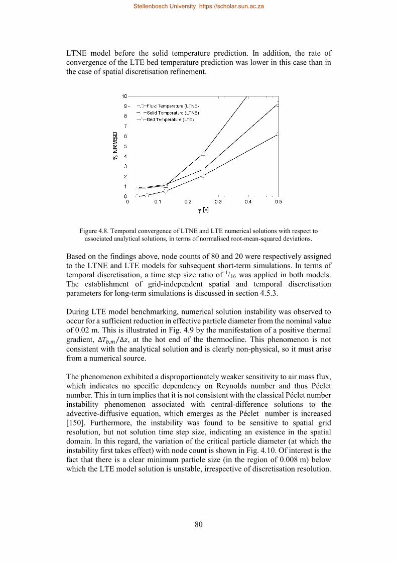
80

LTNE model before the solid temperature prediction. In addition, the rate of convergence of the LTE bed temperature prediction was lower in this case than in the case of spatial discretisation refinement.

Figure 4.8. Temporal convergence of LTNE and LTE numerical solutions with respect to associated analytical solutions, in terms of normalised root-mean-squared deviations.

Based on the findings above, node counts of 80 and 20 were respectively assigned to the LTNE and LTE models for subsequent short-term simulations. In terms of temporal discretisation, a time step size ratio of 1/16 was applied in both models. The establishment of grid-independent spatial and temporal discretisation parameters for long-term simulations is discussed in section 4.5.3. During LTE model benchmarking, numerical solution instability was observed to occur for a sufficient reduction in effective particle diameter from the nominal value of 0.02 m. This is illustrated in Fig. 4.9 by the manifestation of a positive thermal gradient, ∆𝑁𝑁𝑎𝑎,𝑎𝑎 ∆𝑧𝑧⁄ , at the hot end of the thermocline. This phenomenon is not consistent with the analytical solution and is clearly non-physical, so it must arise from a numerical source. The phenomenon exhibited a disproportionately weaker sensitivity to air mass flux, which indicates no specific dependency on Reynolds number and thus Péclet number. This in turn implies that it is not consistent with the classical Péclet number instability phenomenon associated with central-difference solutions to the advective-diffusive equation, which emerges as the Péclet number is increased [150]. Furthermore, the instability was found to be sensitive to spatial grid resolution, but not solution time step size, indicating an existence in the spatial domain. In this regard, the variation of the critical particle diameter (at which the instability first takes effect) with node count is shown in Fig. 4.10. Of interest is the fact that there is a clear minimum particle size (in the region of 0.008 m) below which the LTE model solution is unstable, irrespective of discretisation resolution.


81

In fact, the critical particle diameter starts to rise beyond a node count of approximately 80 nodes.

Figure 4.9. Manifestation of solution instability in the 20 node LTE model as particle diameter is decreased (Gf = 0.02 kg/(m2 s), t = 3600 s).

Figure 4.10. Variation of critical particle diameter with LTE model node count (Gf = 0.02 kg/(m2s), t = 3600 s).

It is important to note that the above observation is specific to the case of a single bed charging procedure characterised by a step increase in bed inlet temperature as well as the prevailing bed conditions. Nonetheless, it suggests that solution stability should be confirmed when applying the LTE model in both short and long-term bed performance simulations. This is especially important in the case of the latter, as instabilities can accumulate over time and directly impact the simulation of TES system operation.


82

4.5.2 Model Validation Validation of the LTNE and LTE model charge and discharge response was undertaken by comparing model predictions to data measured during the charge and discharge of a high-temperature rock bed test rig [13] developed by Allen [61]. The models were programmed to replicate the bed’s design parameters and the conditions associated with its operation during either process. The experimental bed, containing dolerite rock, had a length of 1.489 m, a cross-sectional area of 0.9781 m2, a mean equivalent particle diameter of 0.039 m, a bed porosity of 0.452. Mass flow rate and air inlet temperature values recorded at 10 s intervals during experimentation were used here for simulation purposes. However, for information purposes, the following mean parameters were calculated from the data: mean air mass flow rates during charging and discharging: 0.283 kg/s and 0.362 kg/s; mean air inlet temperatures during charging and discharging: 269 °C and 30 °C; mean uniform bed temperatures at the start of charging and discharging: 52 °C and 287 °C. Predicted and measured fluid temperature histories at three bed locations are shown for bed charging in Fig. 4.11, and for bed discharging in Fig. 4.12.

Figure 4.11. Measured and predicted temperature histories during bed charging at bed locations of 0.178 m, 0.688 m and 1.244 m in the downward flow direction.

For both modes of operation, the LTNE model predictions show good agreement with the experimental data. The LTE model predictions indicate lower model fidelity, although agreement improves with time during charging and discharging. Inter-model agreement is also shown to improve with time. This observation is consistent with the nature of thermocline progression through the bed. As the thermocline moves past a given location, the inter-phase temperature difference falls as conditions tend towards local thermal equilibrium.


83

Figure 4.12. Measured and predicted temperature histories during bed discharging at bed locations of 0.245 m, 0.801 m and 1.311 m in the upward flow direction.

Furthermore, the rock particle size and air mass flux associated with the test data were larger than those applied in the annual performance simulations undertaken in this study. As per the definition of the inter-phase heat transfer co-efficient, ℎ =𝐷𝐷𝑁𝑁 𝑘𝑘𝑓𝑓 𝐷𝐷𝑝𝑝⁄ , a larger particle size gives rise to a lower rate of heat transfer. A larger air mass flux value results in a faster thermocline progression, which reduces the time available for heat transfer to take place. Both of these factors accentuate the inter-phase temperature difference, leading to a lower level of agreement between the LTNE and LTE models. For validation of the idle response model, comparisons were drawn between bed temperature predictions made by the idle model of Mertens et al. [80] and those of the present model, for the reference case they studied. The reference case considered the thermocline degradation in a semi-industrial scale CSP packed bed during an extended idle period. Their finite volume-based model accounted for environmental heat loss through the cylindrical walls of the bed by means of a uniform overall heat transfer coefficient, 𝑁𝑁𝑡𝑡𝑎𝑎𝑏𝑏𝑏𝑏, of 0.16 W/(m2 K). Heat loss through the ends of the bed was apparently not considered, and they evaluated the stagnant bed conductivity parameter using the elaborate Zehner-Bauer-Schlünder model [151]. In order to capture the environmental heat loss accounted for by Mertens et al., the following term, which is representative of the rate of heat loss through the wall of each bed segment, was subtracted from the right hand side of Eqs. (4.25)-(4.27): ��𝑄𝑏𝑏𝑜𝑜𝑠𝑠𝑠𝑠,𝑎𝑎 = 4 𝑁𝑁𝑡𝑡𝑎𝑎𝑏𝑏𝑏𝑏 �𝑁𝑁𝑎𝑎,𝑎𝑎 − 𝑁𝑁𝑎𝑎𝑎𝑎𝑎𝑎� [𝐷𝐷𝑎𝑎 𝜌𝜌𝑠𝑠 𝑐𝑐𝑠𝑠 (1 − 𝜖𝜖)]⁄ (4.34)

Here, 𝑁𝑁𝑎𝑎𝑚𝑚𝑎𝑎 is the ambient temperature of the adjacent environment, and 4 𝐷𝐷𝑎𝑎⁄ represents the ratio of segment wall surface area to bed cross-sectional area for a


84

bed of circular cross-section. Since Mertens et al. did not expressly indicate that their model accounted for heat loss through the top and bottom of the bed, bed ends were treated as adiabatic in the destratification model investigated here. Thermoclines predicted by both models at 24 h and 48 h after idle commencement are shown if Fig. 4.13, with the end-of-charge thermocline calculated by Mertens et al. serving as the initial condition for the present simulation. Given that different bed conduction correlations are applied in each model, the level of agreement between their predictions at both simulation times is generally good, although a slightly greater discrepancy is observed at the cold end of the bed than at its hot end.

Figure 4.13. Comparison of thermoclines predicted by the present and reference bed idle models at 24 h and 48 h after idle commencement.

To validate the bed pressure drop calculation methodology, comparisons were drawn between pressure drop predictions made by the comprehensive packed bed performance model of Zanganeh et al. [27] and those of the present LTNE and LTE models, for the reference case they studied. The reference case considered the temporal variation of bed pressure drop within a small cylindrical rock bed as it is charged over a period of eight hours. Their model featured finite difference discretisation and very detailed localised treatment of heat loss through the wall and the ends of the bed. Unfortunately, not all of the parameters required to evaluate thermal losses in the manner prescribed by Zanganeh et al. were published. Therefore, to enable comparison between their model and the models presented here, environmental heat loss terms based on a mean overall heat transfer coefficient, of the form shown in Eq. (4.34), were incorporated into the LTNE and LTE energy equations. Mean overall heat transfer coefficients for the top and walls of the reference bed were calculated according to stated cumulative energy losses during charging. In this


85

manner, values of 0.313 W/(m2 K) and 1.05 W/(m2 K), respectively, were obtained. Thermal losses through the bottom of the bed were neglected considering the small difference in temperature between the bed and the ground below. Since validation of the pressure drop calculation methodology was sought, rather than of specific correlations, the heat transfer and pressure drop correlations employed by Zanganeh et al. were applied in the LTNE and LTE models for the purposes of this validation. Figure 4.14 shows the resulting prediction of fluid temperatures at the end of the charging period and the variation of bed pressure drop during the charging period, compared to the reference predictions.

Figure 4.14. Comparison of bed fluid temperature and pressure drop predictions made by the LTNE and LTE models (with thermal loss tuning) to that of Zanganeh et al. [27].

The agreement between temperature distributions is good, especially considering the approximate evaluation of thermal losses. Coincidentally, the LTE model prediction shows better agreement than that of the LTNE model, which slightly over-estimates fluid temperature across the height of the bed. In regard to the pressure drop histories, the level of agreement between the predicted and reference data is shown to be satisfactory. Given the numerous constitutional differences between the model of Zanganeh et al. and the LTNE and LTE models, the present authors are of the view the level of inter-model agreement shown in Fig. 4.14 sufficiently demonstrates the validity of the pressure drop calculation approach applied here. 4.5.3 Annual Performance Simulations Based on the bed inlet temperature and mass flow rate specified for the charging phase (see Table 4.1), bed height was selected such that during operation over the course of the year, bed outlet temperature did not exceed 120 °C. This assessment


86

was based on an annual simulation using the 80 node LTNE model with a time step size of 225 s, as per the single-cycle grid-independent discretization parameters. An annual simulation starting with a uniform bed temperature of 20 °C was conducted to determine a realistic initial bed temperature distribution for a subsequent representative annual simulation, based on the distribution determined at 24h00 on 31 December. A representative annual simulation was then run and the maximum bed outlet temperature during the course of the year was identified. During subsequent simulations, bed height was reduced until a bed outlet temperature just beneath the 120 °C threshold was reached. According to this approach, a minimum bed height of 15 m was determined. Three measures of annual TES system performance and a single measure of computational cost were evaluated. System performance was assessed in terms of the cumulative exergy delivered by the rock bed, number of power generation hours, and the cumulative work required to blow air through the bed during both charging and discharging. The importance of these parameters in the context of predicting overall plant performance is highlighted in section 4.2. Exergy delivered by the rock bed during discharge was evaluated according to the properties of the air leaving the bed during discharge – considered to remain constant for each hour of the simulation – relative to the dead state (𝑁𝑁0 = 25 °C and 𝑝𝑝0 = 1.013 bar). Given the low air velocity and density, kinetic and potential contributions were disregarded. The exergy delivered by the bed over the course of a year (8760 hours) can be expressed in discrete form as:

𝑋𝑋𝑓𝑓,𝑎𝑎𝑛𝑛𝑛𝑛 = ��3600 ��𝑋𝑓𝑓𝑛𝑛�8760

𝑛𝑛=1

(4.35)

Here, ��𝑋𝑓𝑓𝑛𝑛 denotes the rate at which exergy is yielded by the bed at a given simulation hour during discharging, as indicated by the subscript 𝑡𝑡. This rate term is calculated according to Eq. (4.36) on the basis of live- and dead-state specific enthalpies and specific entropies for air evaluated using the appropriate EES property functions. ��𝑋𝑓𝑓𝑛𝑛 = ��𝑚𝑓𝑓

𝑛𝑛 ��ℎ𝑓𝑓𝑛𝑛 − ℎ𝑓𝑓,0� − 𝑁𝑁0 �𝑠𝑠𝑓𝑓𝑛𝑛 − 𝑠𝑠𝑓𝑓,0�� (4.36) Generation time was calculated simply by summing the number of hours during the course of the year for which a non-zero discharge mass flow rate was registered. Cumulative blowing work, for both the charge and discharge operating modes, was calculated in a similar fashion to cumulative exergy. In discrete form, annual blowing work can be determined by:

𝑊𝑊𝑎𝑎𝑏𝑏𝑜𝑜,𝑎𝑎𝑛𝑛𝑛𝑛 = ��3600 ��𝑊𝑎𝑎𝑏𝑏𝑜𝑜𝑛𝑛 �

8760

𝑛𝑛=1

(4.37)


87

Here, the blowing power and the overall pressure drop across the bed associated with a given simulation hour are respectively defined as: ��𝑊𝑎𝑎𝑏𝑏𝑜𝑜

𝑛𝑛 = ��𝑚𝑓𝑓𝑛𝑛 ∆𝑝𝑝𝑎𝑎𝑛𝑛 𝜌𝜌𝑓𝑓𝑛𝑛� (4.38)

∆𝑝𝑝𝑎𝑎𝑛𝑛 = � ∆𝑝𝑝𝑎𝑎𝑛𝑛𝑛𝑛

𝑎𝑎=1

(4.39)

In Eq. (4.38), air density is evaluated at the air outlet temperature and pressure during charging, and the air inlet temperature and pressure during discharging. The term ∆𝑝𝑝𝑎𝑎𝑛𝑛 is the overall bed pressure drop, evaluated as the summation of the pressure drops predicted in each bed segment, based on segment-specific values for apparent friction factor, fluid density and superficial velocity. Since the apparent friction factor is a function of Reynolds number, the Reynolds number must also be evaluated for each segment. Finally, the computational cost of each annual TES system simulation is quantified by the model solution time as indicated by EES, with the same computational resources being applied for each analysis. In this regard, computations were undertaken using a 64-bit PC featuring 2.8 GHz Intel Core i7 CPUs in quad-core configuration and 10 GB of RAM. Before conducting comparative annual simulations, solution convergence for the simulation of long-term bed operation was assessed, to determine if grid-independence for annual simulations could be suitably indicated by grid-independence observed in single-cycle simulations. For this purpose, LTNE models with node counts of 80 – 240 nodes, and LTE models with node counts of 40 – 280 nodes were applied in year-long simulations. The 20 node LTE model solution diverged early in the simulation and therefore could not be considered. The respective upper node count limits were imposed by restrictions to the number of problem variables allowed by the EES software. Solution convergence associated with three performance measures – annual blowing work, exergy yield and generation time – is shown in Figs. 4.15-4.17 with respect to spatial and temporal discretisation refinements. Convergence is respectively indicated in terms of deviation from solutions obtained for the highest node count and smallest time step size models. That is, the 240 node / 225 s LTNE model and the 280 node / 225 s LTE model. In general, the results indicate that solution convergence requires marked further refinement in spatial discretisation for both the LTNE and LTE models. This clearly demonstrates that under the prevailing conditions, single-cycle grid-independent discretisation parameters cannot be used to achieve converged solutions for annual simulations. This is an important observation that has not been reported in the literature before.


88

Figure 4.15. Deviation in annual blowing work predictions as a function of node count and time step size for the LTNE and LTE models.

Figure 4.16. Deviation in annual exergy yield predictions as a function of node count and time step size for the LTNE and LTE models.

With regard to annual blowing work predictions, shown in Fig. 4.15, thorough convergence in the LTE solutions is indicated for the 225 s and 900 s solutions in the region of approximately 240 nodes, although solution instability limited the 3600 s solution to 200 nodes. Very good agreement between the 225 s and 900 s solutions can be observed for both models. It is apparent that for the LTNE solutions, full convergence is not achieved before the 240 node limit. Also of interest is the fact that the starting deviation in the LTNE solutions is significantly higher than that of the LTE solutions.


89

In terms of annual exergy yield predictions, shown in Fig. 4.16, thorough convergence is achieved for all time step sizes between 200 and 280 nodes, and there is excellent overall agreement between the 225 s and 900 s solutions. In this instance, however, the starting deviation in the LTE solutions is substantially higher than that of the LTNE models. With respect to annual generation time predictions, shown in Fig. 4.17, thorough convergence was achieved by both models for all levels of temporal resolution, apart from for the 3600 s LTNE solution. It is unclear if this solution starts to diverge at 160 nodes given that solutions couldn’t be obtained for node counts of greater than 240 nodes. Once again, excellent overall agreement between the 225 s and 900 s solutions is observed in all instances. Of particular interest is the fact that the lowest spatial resolution LTNE solutions all predict generation times of within one percent of the converged LTNE solution.

Figure 4.17. Deviation in annual generation time predictions as a function of node count and time step size for the LTNE and LTE models.

In reference to the results depicted in Figs. 4.15-4.17, the LTE model was shown to achieve suitable convergence with respect to all three annual performance measures for a node count of 240 and a time step size of 900 s. Although the LTNE model achieved convergence in its prediction of exergy yield and generation time, the node limit imposed upon the model by EES prevented it from reaching converged solutions for blowing work. Considering the importance of this parameter, it was decided that the highest-resolution LTNE model (240 nodes, 225 s) be used in subsequent annual simulations in order to mitigate discretisation error. A very important design parameter affected by the use of non-converged discretisation parameters in annual performance simulations, is bed height. Figure 4.18 shows thermoclines predicted by the converged LTNE and LTE models, in addition to those predicted by LTNE and LTE models discretised as per the single-cycle grid-independent parameters. A node count of 40, instead of 20, was used for the low-resolution LTE model to avoid solution instability. In this regard, evidence


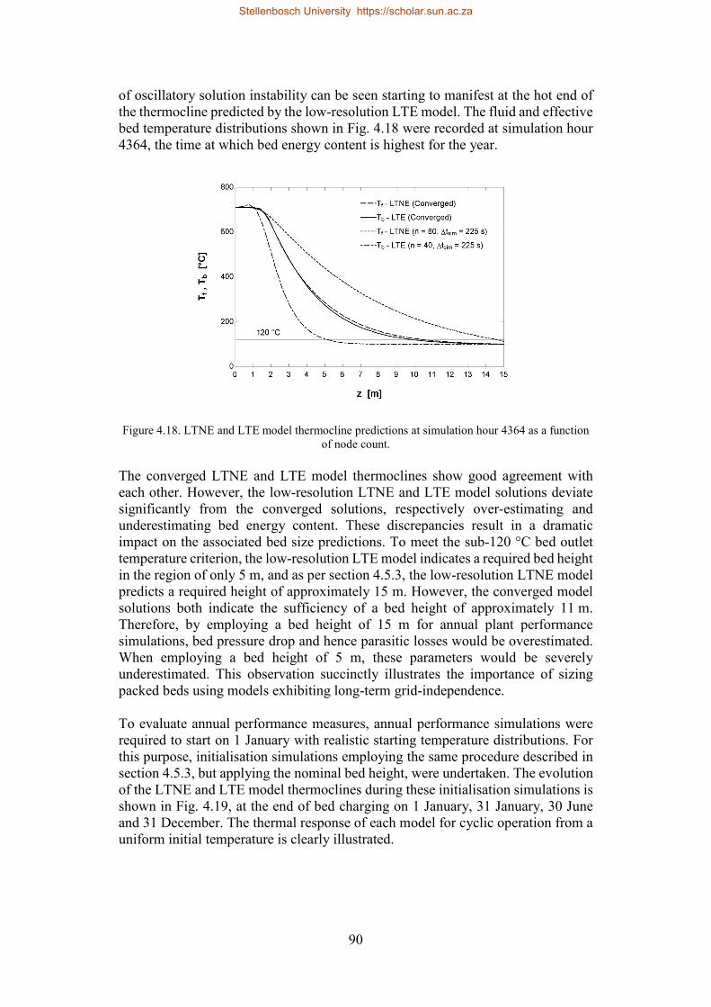
90

of oscillatory solution instability can be seen starting to manifest at the hot end of the thermocline predicted by the low-resolution LTE model. The fluid and effective bed temperature distributions shown in Fig. 4.18 were recorded at simulation hour 4364, the time at which bed energy content is highest for the year.

Figure 4.18. LTNE and LTE model thermocline predictions at simulation hour 4364 as a function of node count.

The converged LTNE and LTE model thermoclines show good agreement with each other. However, the low-resolution LTNE and LTE model solutions deviate significantly from the converged solutions, respectively over-estimating and underestimating bed energy content. These discrepancies result in a dramatic impact on the associated bed size predictions. To meet the sub-120 °C bed outlet temperature criterion, the low-resolution LTE model indicates a required bed height in the region of only 5 m, and as per section 4.5.3, the low-resolution LTNE model predicts a required height of approximately 15 m. However, the converged model solutions both indicate the sufficiency of a bed height of approximately 11 m. Therefore, by employing a bed height of 15 m for annual plant performance simulations, bed pressure drop and hence parasitic losses would be overestimated. When employing a bed height of 5 m, these parameters would be severely underestimated. This observation succinctly illustrates the importance of sizing packed beds using models exhibiting long-term grid-independence. To evaluate annual performance measures, annual performance simulations were required to start on 1 January with realistic starting temperature distributions. For this purpose, initialisation simulations employing the same procedure described in section 4.5.3, but applying the nominal bed height, were undertaken. The evolution of the LTNE and LTE model thermoclines during these initialisation simulations is shown in Fig. 4.19, at the end of bed charging on 1 January, 31 January, 30 June and 31 December. The thermal response of each model for cyclic operation from a uniform initial temperature is clearly illustrated.


91

Figure 4.19. End-of-charge thermoclines predicted by the LTNE and LTE models during initialisation simulations, for 1 January, 31 January, 30 June and 31 December.

Throughout the development of the thermocline, LTE temperature predictions track those of the LTNE model well, although equivalent fluid temperature is consistently under-estimated across most of the bed by the LTE model. After one cycle, the temperature discrepancy between models is fairly minor, although by the end of January, the discrepancy has grown, and remains at a similar magnitude at the mid-year and year-end points. Corresponding thermoclines predicted during the course of the annual performance simulations, which follow on from the initialisation simulations referred to above, are depicted in Fig. 4.20. For the sake of clarity, only predictions for 30 June and 31 December are shown.

Figure 4.20. End-of-charge thermoclines predicted by the LTNE and LTE models during annual performance simulations, for 30 June and 31 December.


92

In general form, the LTE thermoclines are shown to correspond well to the LTNE thermoclines at the seasonal extremes, although equivalent fluid temperatures are again under-predicted; albeit to a lesser extent than in the case of the initialisation simulations. For the annual operation of the bed with nominal parameters, performance measures predicted by the converged LTNE and LTE models are presented in Table 4.2.

Table 4.2. Annual performance measure comparison for the nominal bed.

Performance Measure LTE Model LTNE Model Deviation Exergy Yield [J] 5.75E+14 5.73E+14 +0.4 % Generation Time [h] 1055 1062 -0.7 % Blowing Work [J] 3.42E+12 3.50E+12 -2.1 % Simulation Time [s] 6234 19047 -67 %

By far the greatest deviation between models is in respect of solution time, with the LTE model requiring only a third of the time required by the LTNE model to complete an annual simulation under nominal conditions. The annual exergy yield and annual generation time predictions made by the LTE model show excellent agreement with the associated LTNE model results, with discrepancies of within 1 % observed. The LTE model under-estimates the annual required blowing work more substantially, although the level of agreement with LTNE model is still good. In reference to Figs. 4.20 and 4.21, it is likely that this discrepancy arises from the consistent under-estimation of equivalent fluid temperature. This results in the evaluation of a higher mean fluid density and a lower mean fluid viscosity, and as per Eqs. (4.17) - (4.19), these two effects combine to result in a reduction of bed pressure drop. In this regard, the absolute deviation of the LTE pressure drop prediction from that of the LTNE model is shown in Figure 4.22, for each hour of the annual performance simulations. The high peaks in excess of ±400 Pa indicate hours at which one model has operated in discharge mode when the other has not. For the majority of the year, the LTE model is shown to predict a lower bed pressure drop than the LTNE model. Such instances correlate to times at which the LTE thermocline lies beneath the LTNE thermocline; that is, the LTE model under-estimates the equivalent bed temperature. On a very limited number of occasions, the converse condition exists. To illustrate the impact that the over-estimation of bed height has on annual performance, simulations were run for a bed height of 11 m, approximately indicated by the converged LTNE and LTE models to be the minimum bed height required (Fig. 4.19). Comparative thermodynamic performance results are shown in Table 4.3.


93

Figure 4.21. Hourly deviation of LTE model bed pressure drop prediction from that of the LTNE model during annual performance simulations of the nominal bed.

Table 4.3. Annual performance measure comparison for the reduced-height, 11 m bed.

Performance Measure LTE Model LTNE Model Deviation Exergy Yield [J] 5.75E+14 5.73E+14 +0.4 % Generation Time [h] 1053 1061 -0.8 % Blowing Work [J] 2.76E+12 2.70E+12 +2.5 %

In this instance, exergy yield and generation time deviations are almost identical to those calculated for the nominal bed height of 15 m, although the required blowing work is now slightly over-estimated by the LTE model. Inspection of Fig. 4.22, which is analogous to Fig. 4.21, indicates that for the vast majority of the year, the LTE thermocline lies above the LTNE thermocline for the revised bed conditions, as per the infrequent negative deviations. Of particular importance, however, is the fact that blowing work is indicated to be markedly lower for the reduced-height bed; in the order of 23 % and 19 % for the LTNE and LTE models, respectively. Blowing work reductions of this magnitude would likely have an appreciable effect on overall plant performance predictions. This observation emphasises the importance of sizing rock beds using properly-converged models. To establish the impact that the variation of key bed design parameters would have on the level of inter-model agreement, sensitivities of performance measure deviations to changes in charging temperature, design mass flux, particle size and rock type were assessed. This exercise was undertaken in order to evaluate the general applicability of the LTE model under conditions different to the nominal conditions considered above. The resulting sensitivity characteristics are shown in Figs. 4.23-4.25 as well as Fig. 4.27, with deviations again being expressed as the


94

deviation of converged LTE model outputs from those of the converged LTNE model.

Figure 4.22. Hourly deviation of LTE model bed pressure drop prediction from that of the LTNE model during annual performance simulations of the shortened, 11 m bed.

Figure 4.23 illustrates the sensitivity of performance measure deviations to changes in bed charging temperature over the range 560 °C to 760 °C. As can be seen, deviations in annual exergy yield, generation time and blowing work all show very weak sensitivity to charging temperature, lying within bandwidths of 0.5 %, 0.8 % and 0.6 %, respectively. No substantial trends can be observed in the performance measures as the bed charging temperature is varied.

Figure 4.23. Deviation of LTE model predictions from LTNE model predictions for annual exergy yield, generation time and blowing work, as a function of bed charging temperature.


95

Figure 4.24 depicts the sensitivity of performance measure deviations to changes in design-point discharge mass flux over the range 0.1 kg/(m2 s) to 0.3 kg/(m2 s) – representing a 50 % decrease to 50 % increase of the nominal design-point mass flux. Again, annual exergy yield and generation time predictions show very weak sensitivities to the variation of this parameter, with deviation bandwidths of within 0.6 % and 1.0 %, respectively. However, the sensitivity of annual blowing work to variations in mass flux is greater, with a deviation bandwidth of greater than 2.5 %. Furthermore, there is an evident lack of consistency in the LTE model’s prediction of this parameter over the mass flux range considered, with no clear sensitivity trend exhibited.

Figure 4.24. Deviation of LTE model predictions from LTNE model predictions for annual exergy yield, generation time and blowing work, as a function of design-point mass flux for bed

discharge. Figure 4.25 indicates the sensitivity of performance measure deviations to changes in bed particle diameter over the range of 0.01 m to 0.05 m – representing a 50 % decrease to 150 % increase of the nominal particle diameter. The deviation sensitivities associated with annual exergy yield and generation time are again minor, with deviation bandwidths respectively lying within 1.0 % and 0.8 %. The deviation sensitivity exhibited by annual blowing work is much more substantial, however, with a deviation bandwidth in excess of 20 %. This dramatic sensitivity, with the associated transition from an under-prediction to over-prediction of blowing work, indicates a significant variation in the fidelity of the LTE model in predicting bed pressure drop. The source of this variation is a marked change in the discrepancy between the LTE and LTNE thermocline predictions as particle diameter is increase. This phenomenon is illustrated in Fig. 4.26, which, for example, shows the 30 June end-of-charge thermoclines predicted by both models for particle diameters of 0.01 m and 0.05 m.


96

Figure 4.25. Deviation of LTE model predictions from LTNE model predictions for annual exergy yield, generation time and blowing work, as a function of bed particle diameter.

At the lowest particle diameter, the mean equivalent fluid temperature is significantly under-estimated by the LTE model, whereas at the highest diameter, this temperature is conversely over-estimated. This, in turn, leads to substantial under- and over-estimations of fluid superficial velocity and viscosity, and thus bed pressure drop.

Figure 4.26. End-of-charge thermoclines predicted by the LTE and LTNE models for beds containing particles of 0.01 m and 0.05 m in diameter, for 30 June.

Figure 4.27 highlights the sensitivity of performance measure deviations to changes in the bed’s particulate material. Gabbro, limestone and quartzite rock, as studied by Zanganeh [27], were considered in addition to dolerite – the nominal rock type. This exercise enabled deviation sensitivities to variations in key thermophysical


97

properties to be established. As indicated, deviation sensitivities exhibited by annual exergy yield, generation time and blowing work are all weak, with associated deviation bandwidths lying within 0.5 %, 0.4 % and 1.1 %, respectively. This is in spite of fairly significant variations in rock density and thermal conductivity.

Figure 4.27. Performance measure deviations according to rock type. As illustrated in section 4.5.3, in terms of performance measure prediction fidelity, both the LTNE and LTE models demonstrate a substantially weaker sensitivity to time step size than to node count. In conjunction with this, an increase in integration time step size yields an appreciable decrease in the computational cost of annual simulations associated with both models. Therefore, the potential exists for the obtainment of reasonably accurate performance predictions at significantly lower computational cost by applying coarse temporal discretisation. In order to evaluate this cost-reduction potential, simulations using LTNE and LTE models having a time step size of 3600 s and varying node counts were performed. The resulting performance measure deviations are shown in Figs. 4.28 and 4.29. Deviations are indicated with respect to the reference performance predictions of the highest-resolution LTNE model. Compared to the reference LTNE model predictions, the lowest-resolution, 40 node LTE model predicts annual exergy yield to within 6.0 % and generation time to within 4.4 %, although blowing work is under-estimated by almost 15 %. The solution time required by this model is just 3.0 % of the time required to derive the reference LTNE solution. As the node count is increased to maximum of 200 nodes, deviations in exergy yield, generation time and blowing work reduce to 0.7 %, -0.3 % and -5.1 %, respectively, and the solution time required rises to 17 % of the reference solution time.


98

With regard to the lowest-resolution, 80 node LTNE model, annual exergy yield is predicted to within 1.0 % and generation time to within 0.7 %. Blowing work, however, is overestimated by nearly 17 %. Nonetheless, the model derives a solution in under 5 % of the time required by the reference LTNE model. As the node count is increased to maximum of 240 nodes, deviations in exergy yield, generation time and blowing work reduce to 0.1 %, -0.5 % and -3.5 %, respectively, and the solution time required rises to 23 % of the reference solution time.

Figure 4.28. Annual exergy yield and generation time prediction deviations for the 3600 s LTE and LTNE models, as a function of node count.

Figure 4.29. Solution time and annual blowing work prediction deviations for the 3600 s LTE and LTNE models, as a function of node count.


99

4.6 Summary and Conclusion The results of this study provide important insight concerning the application of both the local thermal equilibrium and local thermal non-equilibrium assumptions in the performance modelling of CSP packed bed TES systems. The use of central differencing to discretise the advective-diffusive LTE energy equation was found to result in numerical solution instability under certain conditions. This manifested in both single-cycle and long-term simulations and primarily exhibited sensitivity to particle diameter and spatial discretisation resolution. The importance of confirming grid-independent spatial discretisation parameters for long-term performance simulations was highlighted. In this regard, it was demonstrated that the application of spatial discretisation parameters derived from converged single-cycle analyses in long-term simulations did not result in solution convergence. However, temporal discretisation resolution could be markedly relaxed in long-term simulations without excessively degrading solution fidelity. The significant consequence of using under-converged models in the sizing of packed beds was also illustrated. Concerning the results correlation between the grid-independent LTE and LTNE models under nominal bed conditions, inter-model agreement in the prediction of annual exergy yield and generation time was found to be excellent. Annual blowing work was slightly under-estimated by the LTE model. This was found to be the result of a consistent under-estimation of the mean equivalent fluid temperature in the bed throughout the year, which in turn led to the evaluation of lower fluid superficial velocities and viscosities, and thus, a lower bed pressure drop. In terms of computational efficiency, the LTE model was able to perform an annual simulation in substantially less time than that required by the LTNE model. Inter-model correlation in the prediction of annual exergy yield and generation time was found to be insensitive to changes in bed charging temperature, discharge mass flux and rock particle diameter, in addition to changes in rock type. Correlation in the prediction of blowing work was found to be weakly sensitive to changes in charging temperature and rock type, although a more significant and erratic sensitivity to mass flux was observed. Furthermore, major sensitivity to variations in rock particle diameter was observed, with the LTE model considerably under- and over-estimating blowing work at the smallest and largest particle sizes considered. This marked sensitivity was found to be the result of significant discrepancies in the thermoclines predicted by either model. Regarding long-term simulation cost-efficiency, it was demonstrated that the solution of both the LTE and LTNE models can be greatly accelerated by using coarse spatial and temporal discretisation resolution. At high node counts, an increase solution time step size only appears to result in a minor degradation of


100

fidelity, whereas at a large solution time step size, the application of lower node counts results in a significant compromise in fidelity. Furthermore, since the use of coarse spatial discretisation was found to result in inaccurate bed sizing, it would appear that the most sensible strategy to improve computational efficiency is to employ fine spatial and coarse temporal discretisation resolutions. With these observations in mind, it can be concluded that for the specific nominal bed parameters considered in this study, the local thermal equilibrium assumption is a reasonable simplifying assumption to apply in long-term packed bed performance simulations. Furthermore, the application of this assumption results in substantial computational cost savings that would be particularly beneficial in multi-simulation parametric or optimisation studies. However, the significant sensitivity of the LTE model’s annual blowing work prediction to rock particle diameter, in addition to the model’s susceptibility to numerical instability under certain conditions, is problematic in the context of the general application of the model. It may be possible to mitigate the problem of numerical instability by discretising the LTE model’s energy equation according to an alternative numerical scheme. Discrepancies in the prediction of blowing work, however, are ultimately inherent to the nature of the local thermal equilibrium assumption. To conclude, therefore, the application of the Effectiveness-NTU LTNE model, with fine spatial but coarse temporal discretisation, appears to offer a more robust means of improving the computational efficiency of long-term rock bed performance simulations without excessively compromising prediction fidelity.


101

5

Performance Characterisation of a Peaking Open Volumetric Receiver CSP Plant Incorporating Rock Bed Thermal Storage 5.1 Abstract The utilisation of open volumetric receivers in concentrating solar power plants offers several potential advantages. However, open volumetric receiver CSP plant technology has not yet enjoyed commercial implementation. This is as a consequence of several technical challenges which must be overcome in order to improve its economic attractiveness. Nonetheless, the technology holds significant potential and is the subject of considerable research attention. In spite of this, the long-term operation and performance of large-scale OVR CSP plants has not been widely addressed. Furthermore, the incorporation of rock bed thermal energy storage systems in such plants has received minimal attention, and the operation of OVR CSP plants for peak power generation purposes does not appear to have been investigated publically in the past at all. The purpose of this work, therefore, is to simulate and evaluate the performance characteristics of a peaking OVR CSP plant incorporating rock bed thermal storage. The study employs custom-developed tools to design a series of OVR CSP plants and subsequently model their annual thermodynamic performance based on detailed system models. In particular, the study seeks to develop a comprehensive understanding of the relationships between plant solar-electric efficiency, energy yield, solar multiple and TES capacity. The resulting performance predictions enable the identification of key behavioural trends and operating characteristics inherent to the technology. 5.2 Introduction One barrier to the improvement of concentrating solar power (CSP) plant performance is the modest maximum allowable temperatures at which mainstream heat transfer fluids, such as molten salt, can operate before degrading. This limit compromises power cycle thermodynamic performance as it moderates the peak working fluid temperature associated with the cycle. The use of air as an alternative heat transfer fluid (HTF) overcomes this difficulty and presents numerous additional advantages. However, the poor heat capacity and


102

low density of air also introduce some significant technical challenges. One of these challenges is the design of solar receivers that are capable of heating air to high temperatures under high solar flux conditions. Open volumetric receivers (OVRs) incorporating porous absorber media have been developed for this purpose, especially for application in central receiver CSP plants that employ water/steam power cycles. The only example of such a plant currently in existence is the 1.5 MWe Solar Tower Jülich pre-commercial OVR plant in Germany [8]. A simplified schematic of an OVR-based water/steam CSP plant is shown in Fig. 1.1 of Chapter 1. In an OVR-type receiver, which appears to have first been conceptualised by Fricker [7], sunlight concentrated by a heliostat field is cast onto an exposed porous absorber surface. The porosity of the absorber permits the penetration of solar radiation and consequently internal, volumetric heating of the absorber material. Concurrently, air from the surrounding atmosphere is drawn through the absorber and is convectively heated by the hot absorber material to a specified outlet temperature. The hot air is then transferred through an HTF distribution network to a heat recovery steam generator (HRSG) to produce steam for the power block, and/or a thermal energy storage (TES) system, with fans being employed to circulate the air. After exiting the HRSG, the cooler air is returned to the OVR where it is exhausted to the atmosphere in close proximity to the absorber. Here, a portion of the return air is re-entrained by the absorber while the rest is lost to the atmosphere. Thermal energy storage can be achieved using a packed bed, containing particulate refractory materials [68] or crushed rock [27], which is incorporated into the HTF distribution network. During charging, hot air emanating from the OVR convectively heats the storage medium as it passes through the bed. When required, heat is subsequently liberated as cooler air is passed through the bed in the reverse direction. The performance of OVR CSP plants has been modelled in a number of prior studies. As detailed in the review by Pitot de la Beaujardiere and Reuter [10], these include investigations associated with the CESA-I and TSA research plants [89,90], the Solar Tower Jülich plant [72,92,152], and plants that have been proposed for construction, such as the original PS10 plant configuration in Spain [30] and the AlSol plant in Algeria [98]. In addition, numerous works have sought to model the performance characteristics of a variety of conceptual plant designs. Several of these have applied the modelling methodologies developed as part of the Virtual Institute of Central Receiver Power Plants initiative [44] for the purposes of performance prediction and optimisation [46,48] and the evaluation of plant control strategies [99]. The performance of OVR


103

plants featuring gas turbine hybridisation [108,111], as well as natural gas [112] and biomass [23] co-firing has also been studied. The performance implications of utilising rock bed thermal storage for applications where air and/or combustion exhaust gases comprise the heat transfer fluid have been investigated by numerous authors. For example, Allen [61] and Heller and Gauché [67] studied the incorporation of rock beds in solarised gas turbine cycles. Zanganeh et al. [27,75,153] and Zavattoni et al. [79] evaluated the operating characteristics and performance of rock beds used in general CSP and process heat applications. In addition, Mertens et al. [80] simulated the performance of a rock bed TES system incorporated in a small OVR CSP plant, and studied the impact of varying bed design parameters on basic, short-duration plant performance. In electricity markets where renewable power production is a priority, the operation of CSP plants in a dispatchable, and in particular, peaking generation role is becoming an attractive financial proposition. This is since market prices for power during this period are high, and because the generation window can be shifted more cost-effectively using TES than employing direct electrical battery storage. For this purpose, rock bed TES technology holds significant potential in view of the low cost of rock compared to engineered thermal media. With this in mind, the utilisation of OVR CSP plants for peaking duty is of potential interest, given that OVR technology permits high power block steam temperatures and can incorporate rock bed TES. These attributes offer the potential for high power block thermal efficiency and low TES capital costs. The overall performance of such a configuration is dependent on key thermodynamic interactions between the constituent plant systems that occur over long periods of time, and requires detailed modelling to predict to any useful degree of fidelity. With this in mind, a review of available literature highlights the lack of research attention that has been given to the OVR/rock bed CSP plant concept. In fact, the authors were unable to identify any prior published research specifically evaluating the operational characteristics of a) OVR CSP plants operating in a peaking role, and b) the annual performance of OVR CSP incorporating rock bed TES. The purpose of this study, therefore, is to comprehensively investigate the thermodynamic performance characteristics of a large-scale OVR CSP plant, whose operation as a peaking generator is enabled by a rock bed TES system. In particular, the primary objectives of the study are to a) provide a benchmark indication of the level of performance that can anticipated from such a plant, and b) establish an understanding of the relationships that exist between plant solar-electric efficiency, energy yield, heliostat field size and TES capacity. For this purpose, a 100 MWe central receiver OVR plant incorporating rock bed TES and designed to operate at Daggett, California in a peaking role is considered.


104

Various plant configurations are evaluated, with design-point parameters determined in each instance using a detailed plant design tool. The annual performance of each configuration is then predicted based on these inputs, an appropriate plant control algorithm and hourly meteorological data, using a quasi-steady plant performance model having the capacity to account for off-design effects. The results of the study provide key, first-time insights concerning plant design, performance and operating characteristics. For all plant configurations considered, solar-electric efficiencies and energy yield are determined as functions of heliostat field size and TES capacity. Furthermore, intra-plant energy transfer and intra-annual variations in electricity output are investigated. In totality, the results of the study enable an initial appraisal of the performance potential of OVR CSP plant technology when applied in such a generation role. 5.3 Modelling Methodology 5.3.1 Plant Operating Strategy The conceptual plant considered in this study is designed to dispatch up to 100 MWe during California’s peak power demand period of 16h00 to 21h00 [154]. During this period, power demand ramps up rapidly as output from the state’s significant photovoltaic power capacity drops-off towards the evening. As such, the plant must possess sufficient TES capacity for power generation to be shifted into the evening. In addition, the plant’s OVR will operate largely out of phase with its water/steam power block (PB), and the majority of its heat supply will be used to charge the TES system, rather than being used directly by the PB. Finally, given the fairly brief dispatch window, the PB will lie idle for at least a significant portion of each day. With these characteristics in mind, as well as the requirement for a PB start-up phase, plant operation can be categorised according to eight specific modes, detailed in Table 5.1. 5.3.2 General Modelling Strategy Plant performance modelling was undertaken in two, sequential stages. The first stage entailed the use of a plant design model to simulate plant performance at the design point, based upon nominal design specifications such as net electrical power generation and ambient conditions. Design-point parameters derived from this model were then incorporated into a second, plant performance model, capable of calculating off-design performance and applied to simulate quasi-steady plant performance over the course of a representative year. The plant models were constituted by coupled, individual system models responsible for the performance prediction of the plant’s heliostat field (HF), open volumetric receiver (OVR), air distribution network (ADN), TES and PB systems.


105

Table 5.1. Modes of plant operation.

# Mode Details Occurrence 1 TES Charging Mode TES system is charged with heat

from OVR Between sunrise and 15h00, if solar radiation is sufficient

2 PB Generation Mode A PB generates power using heat

from both OVR and TES system Between 16h00 and 21h00, if both solar radiation and TES system capacity are sufficient

3 PB Generation Mode B PB generates power using heat from TES system alone

Between 16h00 and 21h00, if TES system capacity is sufficient but solar radiation is insufficient

4 Plant Idle Mode Plant lies idle (apart from auxiliary systems)

Under any alternative conditions

5 PB Start-up Mode A Start-up of PB using heat from both OVR and TES system, air flow through PB at 25 % of full load air mass flow rate, no power generation

Between 15h00 and 16h00, if both solar radiation and TES system capacity are sufficient

6 PB Start-up Mode B Start-up of PB using heat from TES system only, air flow through PB at 25 % of full load air mass flow rate, no power generation

Between 15h00 and 16h00, if TES system capacity is sufficient but solar radiation is insufficient

7 PB Start-up Mode C Start-up of PB using heat from OVR with concurrent TES system charging, air flow through PB at 25 % of full load air mass flow rate, no power generation

Between 15h00 and 16h00, if solar radiation is sufficient and TES system can be charged

8 PB Start-up Mode D Start-up of PB using heat from OVR only, air flow through PB at 25 % of full load air mass flow rate, no power generation

Between 15h00 and 16h00, if solar radiation is at the appropriate level

The plant design model considered a scenario where at the design point, heat input to the PB was provided solely by the receiver, without any contribution from the thermal energy TES system. Thus, the plant design model only incorporated the HF, OVR, ADN and PB system models. Simulations employing the plant performance model were driven by hourly input data derived from the TMY3 typical meteorological year data set [155] for the virtual location of the plant: Daggett, California. Energy and continuity coupling of the system models was achieved by the transfer of key system input and output variables, and plant control decisions were made according to data received from the simulation input data set, and variables generated by the HF and TES system models. The nature and direction of information transfer in the simulation of plant performance is detailed in Fig. 5.1.


106

To maximise computational cost-efficiency, an important consideration in annual CSP plant performance modelling, system models incorporated component performance maps and curves, as well as simplifying assumptions, where appropriate. Furthermore, all programming and simulation work was undertaken in the EES computational environment [123], which enables the iterative solution of complex equation systems.

Figure 5.1. Information transfer in the simulation of plant performance. 5.3.3 System Models A process flow diagram of the plant configuration is provided in Fig. 5.2, and indicates the incorporation of all thermofluid systems; that is, the OVR, ADN, TES and PB systems. System performance is calculated on the basis of thermofluid parameters evaluated at the inlet and outlet nodes of the constituent components of each system. To this end, parameters are determined at 18 air nodes (A) and 12 water/steam nodes (W), as displayed in Fig. 5.2. The OVR and TES systems comprise components lying between nodes A10 and A1, and A2 and A8, respectively. Solar radiation is supplied to the OVR system via the absorber component lying between nodes A13 and A14. The PB system requires both air and water/steam parameters to be evaluated. Its water/steam circuit runs between nodes W1 and W12, while its air circuits through the HRSG and air-cooled condenser (ACC) run between nodes A3 and A7, and A16 and A17, respectively. The steam exit point at node W11 permits blowdown steam to be released. The HF system model is used to predict the solar radiation concentrated onto the OVR, ��𝑄𝑖𝑖𝑛𝑛𝑛𝑛, by the plant’s heliostat field. Since determining the distribution of radiation across the receiver is dependent on detailed design parameters that are not considered in this study, OVR performance was calculated based upon the mean radiation flux. This assumption is concomitant with the exploratory nature of this


107

work. As such, ��𝑄𝑖𝑖𝑛𝑛𝑛𝑛 is calculated as a spatially-independent parameter according to [105]: ��𝑄𝑖𝑖𝑛𝑛𝑛𝑛 = 𝐴𝐴ℎ𝑓𝑓 𝐷𝐷𝑑𝑑𝑛𝑛 𝜂𝜂ℎ𝑓𝑓 (5.1)

Figure 5.2. Plant process flow diagram, incorporating all thermofluid system models. The heliostat mirror surface area, 𝐴𝐴ℎ𝑓𝑓, is calculated by the plant design model, based on the design point net electrical power output of the plant. The direct normal insolation at a given hour, 𝐷𝐷𝑑𝑑𝑛𝑛, is obtained from the TMY 3 data set. During simulation, mean wind speed read from the simulation input data is used as an HF system control variable. At speeds in excess of a maximum allowable value of 17 m/s [94], operation of the heliostat field ceases in order to account for heliostat protection via stowage. Heliostat field power consumption was evaluated as the product of the number of heliostats in the field and the continuous power consumption of each heliostat, taken here to be 55 W [156]. At a given hour, the heliostat field efficiency, 𝜂𝜂ℎ𝑓𝑓, is interpolated from a heliostat field efficiency matrix as a function of the associated solar elevation and azimuth angles. Matrix generation was undertaken using the Solar Power Tower Integrated Layout and Optimization Tool (SolarPILOT) software [157]. SolarPILOT calculates efficiency data based on user inputs of site latitude, design intercept radiation at the receiver and tower height, as well as other more specific parameters. Calculations account for cosine, attenuation, blocking and shading, receiver intercept and mirror reflectivity losses. The non-default parameters applied in the design and simulation of the nominal plant heliostat field are presented in Appendix C.1. The nominal tower height, 𝐻𝐻𝑛𝑛𝑜𝑜𝑡𝑡, in m, is evaluated according to the design point value for ��𝑄𝑖𝑖𝑛𝑛𝑛𝑛, in MW, using the following empirical function [100]: 𝐻𝐻𝑛𝑛𝑜𝑜𝑡𝑡 = 36.7 ��𝑄𝑖𝑖𝑛𝑛𝑛𝑛

0.288 (5.2)


108

Solar elevation and azimuth angles were calculated according to the algorithm presented by Duffie and Beckman [158], based on the equation of time derived by Spencer [159], and as a function of day number, 𝑛𝑛𝑑𝑑𝑎𝑎𝑏𝑏, and local time, 𝑡𝑡𝑏𝑏𝑜𝑜𝑖𝑖. The OVR system model is used to predict the air mass flow rate, ��𝑚𝐴𝐴1, that can be heated by the OVR to the specified outlet temperature, 𝑁𝑁𝐴𝐴1, based on the rate at which heat can be provided to the air by the OVR, ��𝑄𝑜𝑜𝑣𝑣𝑟𝑟. This latter parameter is determined as a function of OVR thermal efficiency, 𝜂𝜂𝑜𝑜𝑣𝑣𝑟𝑟: ��𝑄𝑜𝑜𝑣𝑣𝑟𝑟 = ��𝑄𝑖𝑖𝑛𝑛𝑛𝑛 𝜂𝜂𝑜𝑜𝑣𝑣𝑟𝑟 (5.3)

It is assumed that the OVR under consideration here bears technical resemblance to the receiver employed by the Solar Tower Jülich OVR plant [8]. That is, it is composed of a multitude of comparatively small absorber modules, each comprising an extruded siliconized silicon carbide absorber structure within which radiation absorption occurs. In light of this assumption, and as in the case of a previous work [29], OVR thermal performance is predicted here on the basis of quasi-steady test data associated with the 200 kWth “SolAir” OVR [42], which served as a precursor to the state-of-the-art Solar Tower Jülich OVR. These data were used since the authors were unable to source sufficient performance data associated with the facility’s OVR, as implemented. Applying second-order linear regression, fifty-one data sets were used to derive a performance curve, Eq. (5.4), relating OVR thermal efficiency to specific intercepted radiation, ��𝑄𝑖𝑖𝑛𝑛𝑛𝑛 ��𝑚𝐴𝐴1⁄ [MJ/kg]. These data are presented in Appendix C.2. The relation and the degree of agreement with the test data is illustrated in Fig. 5.3. 𝜂𝜂𝑜𝑜𝑣𝑣𝑟𝑟 = −0.578629��𝑄𝑖𝑖𝑛𝑛𝑛𝑛 ��𝑚𝐴𝐴1⁄ �2 + 0.741229��𝑄𝑖𝑖𝑛𝑛𝑛𝑛 ��𝑚𝐴𝐴1⁄ � + 0.621714 (5.4)

Figure 5.3. OVR thermal efficiency as a function of specific intercepted radiation, fitted to test data for the 200 kWth Solair OVR [42].


109

Equation (5.4) defines the efficiency with which air enthalpy is raised as it traverses the absorber, and does not account for thermal losses arising from the dilution of warm air returned to the receiver with ambient air, as a result of return air losses. This loss is accounted for in the calculation of the enthalpy of air entering the absorber, ℎ𝐴𝐴13, as a function of the fraction of return air that is re-entrained by the absorber, 𝑥𝑥𝑎𝑎𝑟𝑟 = (��𝑚𝐴𝐴13 − ��𝑚𝐴𝐴11) ��𝑚𝐴𝐴13⁄ , and the enthalpy of the atmospheric air in the vicinity of the absorber, ℎ𝐴𝐴12: ℎ𝐴𝐴13 = (1 − 𝑥𝑥𝑎𝑎𝑟𝑟) ℎ𝐴𝐴12 + 𝑥𝑥𝑎𝑎𝑟𝑟 ℎ𝐴𝐴10 (5.5)

In this study, a fixed air return fraction of 0.5 [53] was applied for both design and performance simulations. Although this parameter is, in reality, a function of a variety of design [32] and environmental conditions [50], correlations that are able to characterise these dependencies, even approximately, have yet to be published. As the receiver tower is of significant height, ℎ𝐴𝐴12 is evaluated according to the temperature and pressure in the immediate vicinity of the receiver. These are evaluated as functions of the ground-level ambient temperature and pressure, in units of K and Pa – obtained from the TMY3 data file – using the lapse rate equations proposed by Kröger [129]: 𝑁𝑁𝐴𝐴12 = 𝑁𝑁𝑎𝑎𝑎𝑎𝑎𝑎 − 0.00975 𝐻𝐻𝑛𝑛𝑜𝑜𝑡𝑡 (5.6) 𝑝𝑝𝐴𝐴12 = 𝑝𝑝𝑎𝑎𝑎𝑎𝑎𝑎 (1− 0.00975 𝐻𝐻𝑛𝑛𝑜𝑜𝑡𝑡 𝑁𝑁𝑎𝑎𝑎𝑎𝑎𝑎⁄ )3.5 (5.7)

Knowledge of ℎ𝐴𝐴13 permits the calculation of the mass flow rate of air that can be heated by the OVR to the required outlet enthalpy, ℎ𝐴𝐴1, as per Eq. (5.8). This latter parameter is evaluated as a function of the prescribed outlet temperature. ��𝑚𝐴𝐴1 = ��𝑄𝑜𝑜𝑣𝑣𝑟𝑟 (ℎ𝐴𝐴1 − ℎ𝐴𝐴13)⁄ (5.8)

During simulation, the mean radiation flux incident upon the OVR is used as a system control variable to define the operating envelope of the OVR. In order to limit deep part-load operation of the OVR and air distribution network, OVR operation ceases when the indicated mean flux falls beneath 40 % of the design point value. To prevent OVR damage resulting from excessive radiation flux, mean radiation intercepted by the OVR is limited to a maximum value once the flux exceeds 105 % of the design point value. This operational envelope is defined by the default limits associated with the OVR model featured in the GREENIUS software [160]. Pressure drop through the OVR is assumed to arise from two sources. The first source is the absorber, whilst the second is the ducting, including control orifice plates, through which the hot air flows within the receiver. Absorber pressure drop is determined by a discrete and conservative approximation of the Forchheimer-Darcy equation:


110

Δ𝑝𝑝𝑎𝑎𝑎𝑎𝑠𝑠 = 𝑡𝑡𝑎𝑎𝑎𝑎𝑠𝑠 �𝜇𝜇𝐴𝐴1 ��𝑚𝐴𝐴1

𝑘𝑘1 𝜌𝜌𝐴𝐴1 𝐴𝐴𝑎𝑎𝑎𝑎𝑠𝑠+

��𝑚𝐴𝐴12

𝑘𝑘2 𝜌𝜌𝐴𝐴1 𝐴𝐴𝑎𝑎𝑎𝑎𝑠𝑠2 � (5.9)

Here, 𝑡𝑡𝑎𝑎𝑎𝑎𝑠𝑠 is the absorber thickness, taken to be 0.05 m; 𝜇𝜇𝐴𝐴1 and 𝜌𝜌𝐴𝐴1 are the dynamic viscosity and density of air evaluated at the absorber outlet temperature and pressure; and 𝑘𝑘1 and 𝑘𝑘2 are the permeability and inertial coefficients associated with the cross-sectional geometry of the absorber. These later two parameters were taken as 10-7 m2 and 0.011 m, respectively [31]. Accurate calculation of the pressure drop across the internal ducting of the OVR relies on a detailed knowledge of the geometric design of the ducting, which is beyond the scope of this work. An approximate approach to determining this parameter was therefore used. Based on data published by Grasse et al. [94] concerning the proposed PHOEBUS OVR plant, Heller [161] estimated a receiver ducting pressure drop of 1 kPa at the design point. Although the PHOEBUS OVR technology differs to that considered here, it was assumed that this value is reasonably representative of a typical OVR ducting system. If it can be further assumed that if the ducting system loss coefficient remains constant during operation, the resulting pressure drop at a given air mass flow rate can be approximated by Eq. (5.10), with ∆𝑝𝑝𝑑𝑑𝑑𝑑𝑖𝑖,𝑑𝑑𝑝𝑝 set as 1 kPa.

Δ𝑝𝑝𝑑𝑑𝑑𝑑𝑖𝑖 = ∆𝑝𝑝𝑑𝑑𝑑𝑑𝑖𝑖,𝑑𝑑𝑝𝑝 ��𝑚𝐴𝐴1

��𝑚𝐴𝐴1,𝑑𝑑𝑝𝑝 �2

(5.10)

A further assumption that Eq. (5.10) relies upon is that air density at the outlet of the absorber remains constant, irrespective of OVR thermal load, which is reasonable considering that there are no changes in temperature and only very minor changes in pressure at this location during part-load operation. The overall OVR pressure drop is evaluated as the sum of Δ𝑝𝑝𝑎𝑎𝑎𝑎𝑠𝑠 and Δ𝑝𝑝𝑑𝑑𝑑𝑑𝑖𝑖. The ADN comprises an interconnected system of dampers, fans and ducts (including 90° bends and junctions). The various plant operating modes require the activation of specific flow circuits, which would in reality be achieved by the opening or closing of dampers. For illustrative purposes, Fig. 5.4 identifies the flow paths and thermofluid systems associated with the plant’s primary active modes, modes 1-3. For operation in mode 1, the ADN fan lying between nodes A8 and A9 is used to draw hot air from the OVR through the TES system, thereby charging it. Concurrently, the TES fan lying between nodes A8 and A15 is bypassed by means of damper control. The HRSG side of the ADN is isolated in the same manner. During mode 2 operation, hot air is supplied to the HRSG for PB operation from both the OVR and the now-discharging TES system, in order to provide the required heat input. Accordingly, both fans must be operated, although each only at part-


111

load. Finally, for operation in mode 3, the OVR side of the ADN is isolated, and heat is provided to the HRSG solely from the TES system as it is discharged.

Figure 5.4. Air distribution network configurations for plant operating modes 1-3. Static pressure drops in each ADN configuration are calculated by accounting for losses in the OVR, TES system, HRSG, straight ducts, and 90° mitre bends, where applicable. Pressure drops across flow junctions were neglected. Duct friction factors, 𝑓𝑓𝑑𝑑𝑑𝑑𝑖𝑖, are evaluated using the Colebrook equation for a surface roughness of 0.015, applicable to lightly rusted steel surfaces [129]. The pressure drop associated with each ADN configuration is then calculated as:

∆𝑝𝑝𝐴𝐴𝐴𝐴𝑁𝑁 =12�𝑓𝑓𝑑𝑑𝑑𝑑𝑖𝑖�𝜌𝜌𝑎𝑎,𝑗𝑗 𝑣𝑣𝑎𝑎,𝑗𝑗

2 𝐿𝐿𝑑𝑑𝑑𝑑𝑖𝑖,𝑗𝑗

𝐷𝐷𝑑𝑑𝑑𝑑𝑖𝑖,𝑗𝑗+ 𝑘𝑘𝑎𝑎𝑒𝑒𝑛𝑛�𝜌𝜌𝑎𝑎,𝑗𝑗 𝑣𝑣𝑎𝑎,𝑗𝑗

2 � + ∆𝑝𝑝𝑎𝑎

+ ∆𝑝𝑝ℎ𝑟𝑟𝑠𝑠𝑟𝑟 (5.11)

Here, 𝐿𝐿𝑑𝑑𝑑𝑑𝑖𝑖,𝑗𝑗 and 𝐷𝐷𝑑𝑑𝑑𝑑𝑖𝑖,𝑗𝑗 denote the length and diameter of each straight duct, 𝑛𝑛𝑎𝑎𝑒𝑒𝑛𝑛 and 𝑘𝑘𝑎𝑎𝑒𝑒𝑛𝑛 denote the number of mitre bends and the mitre bend loss coefficient, and 𝜌𝜌𝑎𝑎,𝑗𝑗 and 𝑣𝑣𝑎𝑎,𝑗𝑗 denote the mean air density and mean air velocity within each duct. For duct sizing purposes, this latter parameter was set to be 30 m/s at the design point for both hot and warm ducts. The mitre bend loss coefficient was taken to be 0.25 [129]. The last two terms on the right hand side of Eq. (5.11) manifest if pressure drops across the rock bed and/or HRSG must be accounted for. Based on a conceptual ADN layout, estimates for duct lengths and number of bends for each flow path are provided in Table 5.2, in respect of modes 1-3, for illustrative purposes. Where applicable, these are expressed as functions of tower height and/or rock bed height, 𝐻𝐻𝑎𝑎. Heat loss from the straight ducts is accounted for in a simplified manner, by assuming that duct insulation provides the dominant resistance to heat transfer to the ambient environment, and that the conductivity of the insulation material is temperature-independent. It is further assumed that the thickness of insulation is


112

minor compared to the hot and warm duct diameters. Accordingly, a mean overall heat transfer coefficient can be calculated for the hot and warm ducts duct based on a design-point temperature drop, and hence enthalpy drop, over the length of reference hot and warm ducts. For the hot ducts, the associated heat transfer coefficient is calculated assuming a 5 K temperature drop over the flow path A1-A2:

𝑁𝑁 = ��𝑚𝐴𝐴1,𝑑𝑑𝑝𝑝 (ℎ𝐴𝐴1 − ℎ𝐴𝐴2) �𝐴𝐴𝐴𝐴1−2��𝑁𝑁𝐴𝐴1,𝑑𝑑𝑝𝑝 + 𝑁𝑁𝐴𝐴2,𝑑𝑑𝑝𝑝� 2⁄ − 𝑁𝑁𝑎𝑎𝑎𝑎𝑎𝑎,𝑑𝑑𝑝𝑝��⁄ (5.12)

Table 5.2. Air distribution network flow path details.

Mode Path Estimated Length [m] Number of Bends 1 a. OVR – TES 𝐻𝐻𝑛𝑛𝑜𝑜𝑡𝑡 − 𝐻𝐻𝑎𝑎 + 𝐷𝐷𝑎𝑎 2⁄ + 15 2 b. TES – ADN Fan 𝐷𝐷𝑎𝑎 + 65 9 c. ADN Fan – OVR 𝐷𝐷𝑎𝑎 2⁄ + 𝐻𝐻𝑛𝑛𝑜𝑜𝑡𝑡 + 10 1 2 a. OVR – A2 Junction 𝐻𝐻𝑛𝑛𝑜𝑜𝑡𝑡 − 𝐻𝐻𝑎𝑎 + 𝐷𝐷𝑎𝑎 2⁄ + 10 1 b. A2 Junction – HRSG 𝐷𝐷𝑎𝑎 2⁄ + 15 1 c. HRSG – A8 Junction 𝐷𝐷𝑎𝑎 + 45 2 d. A8 Junction – ADN Fan 𝐷𝐷𝑎𝑎 2⁄ + 15 1 e. ADN Fan – OVR 𝐷𝐷𝑎𝑎 2⁄ + 𝐻𝐻𝑛𝑛𝑜𝑜𝑡𝑡 + 10 1 f. A8 Junction – TES Fan 10 0 g. TES Fan – TES 𝐷𝐷𝑎𝑎 2⁄ + 30 3 h. TES – A2 Junction 5 0 3 a. TES – HRSG 𝐷𝐷𝑎𝑎 2⁄ + 20 2 b. HRSG – TES Fan 𝐷𝐷𝑎𝑎 + 55 3 c. TES Fan – TES 𝐷𝐷𝑎𝑎 2⁄ + 30 3

The same methodology is applied to determine the overall heat transfer coefficient for the warm ducts, by considering flow path A9-A10 and again assuming an allowable design point temperature drop of 5 K. Knowledge of each coefficient then permits the estimation of duct outlet temperatures under all operating conditions. Owing to the operational characteristics of the OVR, air flow through the plant’s two air circulation fans must be varied significantly, and they are consequently required to operate mostly at part-load. In order to maximise off-design efficiency, it is assumed here that the electric motors driving the fans are powered by variable frequency drives (VFDs) in order to permit variable speed fan operation. It is further assumed that the fans are axial in nature and are able to operate at a fixed static efficiency, 𝜂𝜂𝑓𝑓𝑎𝑎𝑛𝑛, of 85 % across the required speed range. This level of performance is consistent with that of state-of-the-art axial fans [162]. The constant fan efficiency simplification is viewed as being reasonable, considering that each fan’s Reynolds number is expected to appreciably exceed 1 x 106, even at low volume flow rates, given their anticipated blade diameter and design point rotational speed. This estimate is based on performance characteristics associated with commercial equipment [162]. Above a Reynolds number of 1 x 106, the static efficiency of aerofoil-bladed fans typically shows negligible dependence on this parameter [163].


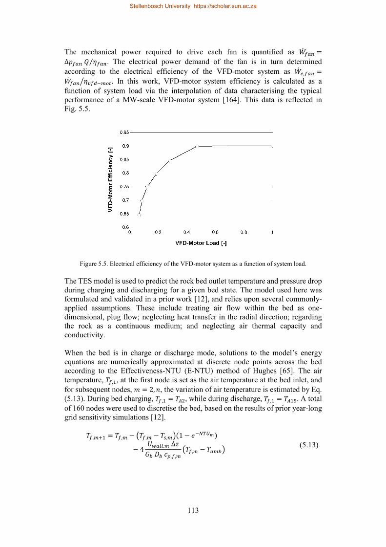
113

The mechanical power required to drive each fan is quantified as ��𝑊𝑓𝑓𝑎𝑎𝑛𝑛 =Δ𝑝𝑝𝑓𝑓𝑎𝑎𝑛𝑛 𝑄𝑄 𝜂𝜂𝑓𝑓𝑎𝑎𝑛𝑛⁄ . The electrical power demand of the fan is in turn determined according to the electrical efficiency of the VFD-motor system as ��𝑊𝑒𝑒,𝑓𝑓𝑎𝑎𝑛𝑛 =��𝑊𝑓𝑓𝑎𝑎𝑛𝑛 𝜂𝜂𝑣𝑣𝑓𝑓𝑑𝑑−𝑎𝑎𝑜𝑜𝑛𝑛� . In this work, VFD-motor system efficiency is calculated as a function of system load via the interpolation of data characterising the typical performance of a MW-scale VFD-motor system [164]. This data is reflected in Fig. 5.5.

Figure 5.5. Electrical efficiency of the VFD-motor system as a function of system load. The TES model is used to predict the rock bed outlet temperature and pressure drop during charging and discharging for a given bed state. The model used here was formulated and validated in a prior work [12], and relies upon several commonly-applied assumptions. These include treating air flow within the bed as one-dimensional, plug flow; neglecting heat transfer in the radial direction; regarding the rock as a continuous medium; and neglecting air thermal capacity and conductivity. When the bed is in charge or discharge mode, solutions to the model’s energy equations are numerically approximated at discrete node points across the bed according to the Effectiveness-NTU (E-NTU) method of Hughes [65]. The air temperature, 𝑁𝑁𝑓𝑓,1, at the first node is set as the air temperature at the bed inlet, and for subsequent nodes, 𝑚𝑚 = 2,𝑛𝑛, the variation of air temperature is estimated by Eq. (5.13). During bed charging, 𝑁𝑁𝑓𝑓,1 = 𝑁𝑁𝐴𝐴2, while during discharge, 𝑁𝑁𝑓𝑓,1 = 𝑁𝑁𝐴𝐴15. A total of 160 nodes were used to discretise the bed, based on the results of prior year-long grid sensitivity simulations [12].

𝑁𝑁𝑓𝑓,𝑎𝑎+1 = 𝑁𝑁𝑓𝑓,𝑎𝑎 − �𝑁𝑁𝑓𝑓,𝑎𝑎 − 𝑁𝑁𝑠𝑠,𝑎𝑎�(1− 𝑅𝑅−𝑁𝑁𝑇𝑇𝑁𝑁𝑎𝑎)

− 4𝑁𝑁𝑡𝑡𝑎𝑎𝑏𝑏𝑏𝑏,𝑎𝑎 ∆𝑧𝑧𝐺𝐺𝑎𝑎 𝐷𝐷𝑎𝑎 𝑐𝑐𝑝𝑝,𝑓𝑓,𝑎𝑎

�𝑁𝑁𝑓𝑓,𝑎𝑎 − 𝑁𝑁𝑎𝑎𝑎𝑎𝑎𝑎� (5.13)


114

Here, the fluid mass flux within the bed is defined as 𝐺𝐺𝑎𝑎 = ��𝑚𝑓𝑓 𝐴𝐴𝑎𝑎,𝑖𝑖⁄ , where 𝐴𝐴𝑎𝑎,𝑖𝑖 is the cross-sectional area of the rock bed. The number of transfer units parameter associated with each segment, of height ∆𝑧𝑧, is evaluated as 𝐷𝐷𝑁𝑁𝑁𝑁𝑎𝑎 =ℎ𝑣𝑣,𝑒𝑒𝑓𝑓𝑓𝑓,𝑎𝑎 ∆𝑧𝑧 �𝐺𝐺𝑎𝑎 𝑐𝑐𝑝𝑝,𝑓𝑓,𝑎𝑎�⁄ . The term on the far right of Eq. (5.13) accounts for heat loss from the bed to the ambient environment, assuming the bed is circular in cross-section. The temporal variation of the rock temperature is in turn calculated by integrating


𝑎𝑎𝑡𝑡=𝐻𝐻𝑎𝑎Δ𝑧𝑧

1𝜏𝜏𝑎𝑎

(𝑁𝑁𝑓𝑓,𝑎𝑎 − 𝑁𝑁𝑠𝑠,𝑎𝑎)(1− 𝑅𝑅−𝑁𝑁𝑇𝑇𝑁𝑁𝑎𝑎) (5.14)

where the time constant for each segment is given by 𝜏𝜏𝑎𝑎 = 𝜌𝜌𝑠𝑠 (1 − 𝜖𝜖) 𝐻𝐻𝑎𝑎 𝑐𝑐𝑠𝑠,𝑎𝑎/(𝐺𝐺𝑎𝑎 𝑐𝑐𝑝𝑝,𝑓𝑓,𝑎𝑎). Numerical integration was undertaken using EES’s semi-implicit predictor-corrector integral function. A time step size of 3600 s (i.e. 1 hour) was applied to provide acceptably converged solutions, again based on the findings of prior year-long simulations. When the bed is in idle mode, it is assumed that the air at a given location in the bed quickly takes on the temperature of the local rock, given air’s comparatively low specific heat capacity. That is to say, 𝑁𝑁𝑓𝑓,𝑎𝑎 = 𝑁𝑁𝑠𝑠,𝑎𝑎. Assuming no air advection within the bed, time rates of temperature change at the inlet, interior and outlet nodes can be expressed by the semi-discrete Eqs. (5.15)-(5.17), which have been derived by means of central difference discretisation in conjunction with Danckwerts-type boundary conditions. Again, the term on the far right of each of these equations accounts for bed heat loss.

𝑎𝑎𝑁𝑁𝑠𝑠,1

𝑎𝑎𝑡𝑡=

2 𝑘𝑘𝑒𝑒𝑓𝑓𝑓𝑓,10

𝜌𝜌𝑠𝑠 𝑐𝑐𝑠𝑠,1(1 − 𝜖𝜖) �𝑁𝑁𝑠𝑠,2 − 𝑁𝑁𝑠𝑠,1

(∆𝑧𝑧)2 �

− 4𝑁𝑁𝑡𝑡𝑎𝑎𝑏𝑏𝑏𝑏,1

𝐷𝐷𝑎𝑎 𝜌𝜌𝑠𝑠 𝑐𝑐𝑠𝑠,1(1− 𝜖𝜖) �𝑁𝑁𝑠𝑠,1 − 𝑁𝑁𝑎𝑎𝑎𝑎𝑎𝑎� (5.15)


𝑎𝑎𝑡𝑡=

𝑘𝑘𝑒𝑒𝑓𝑓𝑓𝑓,𝑎𝑎0

𝜌𝜌𝑠𝑠 𝑐𝑐𝑠𝑠,𝑎𝑎(1− 𝜖𝜖) �𝑁𝑁𝑠𝑠,𝑎𝑎+1 − 2 𝑁𝑁𝑠𝑠,𝑎𝑎 + 𝑁𝑁𝑠𝑠,𝑎𝑎−1

(∆𝑧𝑧)2 �

− 4𝑁𝑁𝑡𝑡𝑎𝑎𝑏𝑏𝑏𝑏,𝑎𝑎

𝐷𝐷𝑎𝑎 𝜌𝜌𝑠𝑠 𝑐𝑐𝑠𝑠,𝑎𝑎(1− 𝜖𝜖) �𝑁𝑁𝑠𝑠,𝑎𝑎 − 𝑁𝑁𝑎𝑎𝑎𝑎𝑎𝑎� (5.16)

𝑎𝑎𝑁𝑁𝑠𝑠,𝑛𝑛

𝑎𝑎𝑡𝑡=

2 𝑘𝑘𝑒𝑒𝑓𝑓𝑓𝑓,𝑛𝑛0

𝜌𝜌𝑠𝑠 𝑐𝑐𝑠𝑠,𝑛𝑛(1− 𝜖𝜖) �𝑁𝑁𝑠𝑠,𝑛𝑛−1 − 𝑁𝑁𝑠𝑠,𝑛𝑛

(∆𝑧𝑧)2 �

− 4𝑁𝑁𝑡𝑡𝑎𝑎𝑏𝑏𝑏𝑏,𝑛𝑛

𝐷𝐷𝑎𝑎 𝜌𝜌𝑠𝑠 𝑐𝑐𝑠𝑠,𝑛𝑛(1− 𝜖𝜖) �𝑁𝑁𝑠𝑠,𝑛𝑛 − 𝑁𝑁𝑎𝑎𝑎𝑎𝑎𝑎� (5.17)

In both of the above sets of discretised energy equations, thermophysical properties are evaluated at the mean segment temperature and pressure. During charging or discharging, thermally-diffusive effects attributable to radiative conduction are


115

incorporated into the E-NTU equations by means of superposition, as per the findings of Riaz [144], such that:

1 ℎ𝑣𝑣,𝑒𝑒𝑓𝑓𝑓𝑓,𝑎𝑎⁄ = 1 ℎ𝑣𝑣,𝑖𝑖,𝑎𝑎⁄ + 𝑘𝑘𝑟𝑟𝑎𝑎𝑑𝑑,𝑎𝑎 �𝐺𝐺𝑎𝑎2 𝑐𝑐𝑝𝑝,𝑓𝑓,𝑎𝑎2 �⁄ (5.18)

The radiative conductivity, 𝑘𝑘𝑟𝑟𝑎𝑎𝑑𝑑,𝑎𝑎, is calculated according to a correlation provided by Wakao and Kaguei [140], as a function of the rock temperature:

𝑘𝑘𝑟𝑟𝑎𝑎𝑑𝑑,𝑎𝑎 = 0.707 𝑘𝑘𝑓𝑓,𝑎𝑎 �𝑘𝑘𝑠𝑠 𝑘𝑘𝑓𝑓,𝑎𝑎⁄ �1.11 �4 𝜎𝜎 𝑁𝑁𝑠𝑠,𝑎𝑎

3

2 (1 𝜀𝜀 − 1⁄ ) + 1 0.576⁄ 𝐷𝐷𝑝𝑝𝑘𝑘𝑠𝑠�0.96

(5.19)

In accordance with Jefferson’s [145] findings, the volumetric heat transfer coefficient, ℎ𝑣𝑣,𝑖𝑖,𝑎𝑎, featured in Eq. (5.18) is corrected to account for intra-particle heat conduction and is calculated as ℎ𝑣𝑣,𝑖𝑖,𝑎𝑎 = ℎ𝑣𝑣,𝑎𝑎 �1 + 𝐵𝐵𝐵𝐵𝑝𝑝,𝑎𝑎 5⁄ �⁄ . Here, the local particle Biot number is evaluated as 𝐵𝐵𝐵𝐵𝑝𝑝,𝑎𝑎 = ℎ𝑎𝑎 𝐷𝐷𝑝𝑝 2𝑘𝑘𝑠𝑠⁄ , where the local heat transfer coefficient is determined by ℎ𝑎𝑎 = 𝐷𝐷𝑁𝑁𝑎𝑎 𝑘𝑘𝑓𝑓,𝑎𝑎 𝐷𝐷𝑝𝑝⁄ , and 𝐷𝐷𝑝𝑝 is the mean equivalent particle diameter, taken as 0.02 m in this study. The volumetric heat transfer coefficient is calculated as the product of ℎ𝑎𝑎 and 𝑎𝑎, the particle surface area per unit volume of the bed, which, for particles that are considered to be spherical, is given by 𝑎𝑎 = 6(1 − 𝜖𝜖) 𝐷𝐷𝑝𝑝⁄ . The local Nusselt number, 𝐷𝐷𝑁𝑁𝑎𝑎, is predicted by a correlation provided by Wakao et al. [146], as a function of the flow’s Prandtl number, 𝑃𝑃𝑃𝑃𝑎𝑎, and particle Reynolds number, 𝑅𝑅𝑅𝑅𝑝𝑝,𝑎𝑎 = 𝐺𝐺𝑎𝑎 𝐷𝐷𝑝𝑝 𝜇𝜇𝑓𝑓,𝑎𝑎⁄ :

𝐷𝐷𝑁𝑁𝑎𝑎 = 2 + 1.1𝑃𝑃𝑃𝑃𝑎𝑎1/3 𝑅𝑅𝑅𝑅𝑝𝑝,𝑎𝑎

0.6 (5.20) Applicable to Eqs. (5.15)-(5.17), the effective idle bed conductivity is defined as 𝑘𝑘𝑒𝑒𝑓𝑓𝑓𝑓,𝑎𝑎0 = 𝑘𝑘𝑖𝑖𝑜𝑜𝑛𝑛,𝑎𝑎

0 + 𝑘𝑘𝑟𝑟𝑎𝑎𝑑𝑑,𝑎𝑎, with the idle bed conductivity itself, 𝑘𝑘𝑖𝑖𝑜𝑜𝑛𝑛,𝑎𝑎0 , being defined

according to Wakao and Kaguei [140] as:

𝑘𝑘𝑖𝑖𝑜𝑜𝑛𝑛,𝑎𝑎0 =

2 𝑘𝑘𝑓𝑓,𝑎𝑎

1 − 𝑘𝑘𝑓𝑓,𝑎𝑎 𝑘𝑘𝑠𝑠⁄ �ln�𝑘𝑘𝑠𝑠 𝑘𝑘𝑓𝑓,𝑎𝑎⁄ �1 − 𝑘𝑘𝑓𝑓,𝑎𝑎 𝑘𝑘𝑠𝑠⁄ − 1� (5.21)

The pressure drop across the bed is calculated as the sum of the respective bed segment pressure drops, which are in turn calculated as the sum of the static pressure drop and buoyancy pressure difference contribution associated with each segment:

∆𝑝𝑝𝑎𝑎 =34

𝑓𝑓𝑎𝑎𝑝𝑝,𝑎𝑎 ∆𝑧𝑧 𝜌𝜌𝑓𝑓,𝑎𝑎 𝑣𝑣𝑠𝑠,𝑎𝑎

2 (1 − 𝜖𝜖)𝜖𝜖3 𝐷𝐷𝑝𝑝

+ �𝜌𝜌𝑓𝑓,𝑎𝑎+1 − 𝜌𝜌𝑓𝑓,𝑎𝑎� 𝑔𝑔 ∆𝑧𝑧 (5.22)

where the local superficial velocity is determined by 𝑣𝑣𝑠𝑠,𝑎𝑎 = ��𝑚𝑓𝑓 �𝜌𝜌𝑓𝑓,𝑎𝑎 𝐴𝐴𝑎𝑎,𝑖𝑖�⁄ , and the local apparent friction factor is estimated using an empirical correlation derived by Allen [62] for crushed rock that is poured into a packed bed in the axial direction:


116

𝑓𝑓𝑎𝑎𝑝𝑝,𝑎𝑎 = 210 𝑅𝑅𝑅𝑅𝑎𝑎⁄ + 5.9 𝑅𝑅𝑅𝑅𝑎𝑎0.06⁄ (5.23)

Here, the local Reynolds number is evaluated as:

𝑅𝑅𝑅𝑅𝑎𝑎 = 23𝜌𝜌𝑓𝑓,𝑎𝑎 𝑣𝑣𝑠𝑠,𝑎𝑎 𝐷𝐷𝑝𝑝𝜇𝜇𝑓𝑓,𝑎𝑎 (1 − 𝜖𝜖) (5.24)

In regards to bed heat loss, the construction of the bed wall is assumed to comprise an inner refractory liner material, against which the rock particles abut, a steel encasement, and an outer layer of mineral wool insulation. It is further conservatively assumed that the thickness of the insulation is considerably smaller than the diameter of the bed, and that the liner and encasement offer no thermal resistance. The overall heat transfer coefficient of the wall at a given location in the bed can therefore be evaluated as:

𝑁𝑁𝑡𝑡𝑎𝑎𝑏𝑏𝑏𝑏,𝑎𝑎 = 1 �1

ℎ𝑡𝑡𝑎𝑎𝑏𝑏𝑏𝑏,𝑖𝑖,𝑎𝑎+

𝑡𝑡𝑖𝑖𝑛𝑛𝑠𝑠𝑘𝑘𝑖𝑖𝑛𝑛𝑠𝑠,𝑎𝑎

+1

ℎ𝑡𝑡𝑎𝑎𝑏𝑏𝑏𝑏,𝑜𝑜�� (5.25)

In accordance with the approach taken by Heller [66], during bed charging or discharging and bed idle, the local inner wall heat transfer coefficients are respectively determined on the basis of the following Nusselt number correlations:

𝐷𝐷𝑁𝑁𝑡𝑡𝑎𝑎𝑏𝑏𝑏𝑏,𝑎𝑎 = 𝑃𝑃𝑃𝑃𝑎𝑎1/3 𝑅𝑅𝑅𝑅𝑝𝑝,𝑎𝑎

0.61 (5.26) 𝐷𝐷𝑁𝑁𝑡𝑡𝑎𝑎𝑏𝑏𝑏𝑏,𝑎𝑎0 = 20 (5.27)

Convective heat transfer from the insulation to the ambient environment is treated in a simplified manner by assuming a constant local outer wall heat transfer coefficient of 5 W/(m K) [66]. Heat loss through the top and bottom ends of the bed is disregarded. This is since it is assumed that the top of the bed containment has substantial insulation in order to prevent outlet temperature degradation, and that the temperature gradient between the bottom of the containment and the ground beneath it is negligible. From a TES system control perspective, charging of the rock bed was permitted until the bed outlet air temperature exceeded 175 °C. This limit was imposed assuming that the maximum permissible fan inlet temperature would practicably be in the vicinity of this temperature. Discharging of the rock bed was allowed to proceed until a bed outlet air temperature dropped to beneath 650 °C, in view of the lower operating temperature limit of the water/steam cycle. It is well-established that outlet air temperature declines during the discharge of a packed bed TES system, as the thermocline begins to exit the bed. This effect can be mitigated with supplementary fuel firing, or with the inclusion of phase-change


117

TES materials at the bed outlet [88]. However, in plants without such features, the power block must be able to accommodate the fall in HRSG inlet temperature. In the case of conventional combined cycle plants, variations in this parameter are most-effectively managed by operating the water/steam power block in sliding pressure mode - at least for loads above 50 % [124,130]. In CSP applications, fixed and “nozzle section” modes [53], as well as multi-pressure [93] and sliding pressure [80] modes, have been evaluated. However, since mode optimisation is not of concern in this study, power block operation was simulated according to the conventional sliding pressure approach. For off-design conditions, turbine inlet pressure is related to the associated mass flow rate and the design-point parameters according to the well-known ellipse law of Stodola [165]. In the case of the high pressure turbine, for example, inlet pressure is evaluated as

𝑝𝑝𝑊𝑊1 = ��𝑚𝑊𝑊1 ��𝑚𝑊𝑊1,𝑑𝑑𝑝𝑝⁄ �2�𝑝𝑝𝑊𝑊1,𝑑𝑑𝑝𝑝2 − 𝑝𝑝𝑊𝑊2,𝑑𝑑𝑝𝑝

2 �+ 𝑝𝑝𝑊𝑊22 (5.28)

Turbine work output is evaluated solely in terms of the drop in enthalpy across the turbine, according to its associated isentropic efficiency. In the case of the high pressure turbine, for example, specific work output is evaluated as 𝑤𝑤ℎ𝑝𝑝𝑛𝑛 = ℎ𝑊𝑊1 − 𝜂𝜂ℎ𝑝𝑝𝑛𝑛�ℎ𝑊𝑊1 − ℎ𝑊𝑊2,𝑖𝑖𝑠𝑠� (5.29)

Design-point isentropic efficiencies for the high and low pressure turbines are taken as 0.88 and 0.9, as applied by Xiang and Chen [166] for a combined cycle water/steam power block of similar generation capacity. During off-design operation, turbine efficiencies are corrected according to actual steam mass flow rate, using an expression applied by Jüdes et al. [167] and derived from the EBSILON Professional software package [168]. In the case of the high pressure turbine, for example, the off-design efficiency is calculated as:

𝜂𝜂ℎ𝑝𝑝𝑛𝑛 = 𝜂𝜂ℎ𝑝𝑝𝑛𝑛,𝑑𝑑𝑝𝑝 �−1.0176 � ��𝑎𝑊𝑊1��𝑎𝑊𝑊1,𝑑𝑑𝑑𝑑

�4

+ 2.4443 � ��𝑎𝑊𝑊1��𝑎𝑊𝑊1,𝑑𝑑𝑑𝑑

�3−

2.1812 � ��𝑎𝑊𝑊1��𝑎𝑊𝑊1,𝑑𝑑𝑑𝑑

�2

+ 1.0535 � ��𝑎𝑊𝑊1��𝑎𝑊𝑊1,𝑑𝑑𝑑𝑑

�+ 0.701� (5.30)

The isentropic efficiency of the low pressure turbine is corrected for varying turbine outlet steam dryness, evaluated at node W4, by subtracting from Eq. (5.30) the factor �𝑥𝑥𝑟𝑟,𝑊𝑊4,𝑑𝑑𝑝𝑝 − 𝑥𝑥𝑟𝑟,𝑊𝑊4� 2⁄ [167]. At the design point, the dryness fraction at the low pressure turbine outlet was taken to be 0.9. In addition, the live and reheat steam temperatures were set as 585 °C, and the live steam pressure was set 185 bar, as per the design specifications of the state-of-the-art Siemens SST-700 steam turbine, which is suitable for CSP deployment [169].


118

The total shaft power delivered by the turbine set is subsequently calculated as ��𝑊𝑛𝑛𝑜𝑜𝑛𝑛 = 0.99 ��𝑚𝑊𝑊1 𝑤𝑤ℎ𝑝𝑝𝑛𝑛 + ��𝑚𝑊𝑊1 𝑤𝑤𝑏𝑏𝑝𝑝𝑛𝑛(𝑊𝑊3−𝑊𝑊7) + ��𝑚𝑊𝑊4 𝑤𝑤𝑏𝑏𝑝𝑝𝑛𝑛(𝑊𝑊7−𝑊𝑊4)� (5.31)

where the constant 0.99 serves as a power reduction factor to account for mechanical, turbine thrust equalisation, and exhaust losses. The term 𝑤𝑤𝑏𝑏𝑝𝑝𝑛𝑛(𝑊𝑊3−𝑊𝑊7) denotes the specific work derived from the low pressure turbine before the deaerator extraction point, while 𝑤𝑤𝑏𝑏𝑝𝑝𝑛𝑛(𝑊𝑊7−𝑊𝑊4) denotes that derived after the extraction point. The electrical power output of the generator is evaluated as ��𝑊𝑟𝑟𝑒𝑒𝑛𝑛 = 𝜂𝜂𝑟𝑟𝑒𝑒𝑛𝑛 ��𝑊𝑛𝑛,𝑛𝑛𝑜𝑜𝑛𝑛, where at a given load, generator electromechanical efficiency, 𝜂𝜂𝑟𝑟𝑒𝑒𝑛𝑛, is calculated according to the following relationship employed by Patnode [170]:

𝜂𝜂𝑟𝑟𝑒𝑒𝑛𝑛 = 0.9 + 0.258 � ��𝑊𝑡𝑡𝑜𝑜𝑡𝑡��𝑊𝑡𝑡𝑜𝑜𝑡𝑡,𝑑𝑑𝑑𝑑

� − 0.3 � ��𝑊𝑡𝑡𝑜𝑜𝑡𝑡��𝑊𝑡𝑡𝑜𝑜𝑡𝑡,𝑑𝑑𝑑𝑑

�2

+ 0.12 � ��𝑊𝑡𝑡𝑜𝑜𝑡𝑡��𝑊𝑡𝑡𝑜𝑜𝑡𝑡,𝑑𝑑𝑑𝑑

�3 (5.32)

Within the ACC, the rate of heat transfer between the condensing steam and cooling air flows at design or off-design conditions can be quantified by the following three relations:

��𝑄𝑎𝑎𝑖𝑖𝑖𝑖 = ��𝑚𝐴𝐴16(ℎ𝐴𝐴17 − ℎ𝐴𝐴16) (5.33) ��𝑄𝑎𝑎𝑖𝑖𝑖𝑖 = ��𝑚𝑊𝑊4(ℎ𝑊𝑊5 − ℎ𝑊𝑊4) (5.34) ��𝑄𝑎𝑎𝑖𝑖𝑖𝑖 = (𝑁𝑁 𝐴𝐴)𝑎𝑎𝑖𝑖𝑖𝑖 Δ𝑁𝑁𝑏𝑏𝑎𝑎,𝑎𝑎𝑖𝑖𝑖𝑖 (5.35)

Here, the log mean temperature difference, Δ𝑁𝑁𝑏𝑏𝑎𝑎,𝑎𝑎𝑖𝑖𝑖𝑖, is defined as

Δ𝑁𝑁𝑏𝑏𝑎𝑎,𝑎𝑎𝑖𝑖𝑖𝑖 =(𝑁𝑁𝐴𝐴17 − 𝑁𝑁𝑊𝑊4) − (𝑁𝑁𝐴𝐴16 − 𝑁𝑁𝑊𝑊4)

ln[(𝑁𝑁𝐴𝐴17 − 𝑁𝑁𝑊𝑊4) (𝑁𝑁𝐴𝐴16 − 𝑁𝑁𝑊𝑊4)⁄ ] (5.36)

Comprehensive physical modelling of the thermofluid performance of air-cooled condensers (ACC) is complex, and requires site-specific design, using detailed design parameters that enable the accurate prediction of heat transfer, pressure drop and fan performance. Since such detailed analysis is beyond the scope of this study, a simplified approach based on published ACC performance data was applied to predict representative design-point and off-design operating characteristics. It is an approach similar in nature to that employed by Patnode [170].

The reference performance data was obtained from the work of Conradie and Kröger [171], who used their detailed, empirical-based model to predict the thermofluid performance of a typical forced-draft A-frame ACC unit. The unit was described as having a design-point capacity of 11036 kWth at a steam saturation temperature of 59.1 °C and a dry bulb temperature of 15.6 °C. Air leaves the ACC at 37.3 °C and at a mass flow rate of 540.8 kg/s. Under these conditions,


119

condensation occurs at a log mean temperature difference of approximately 31.4 K, yielding a 𝑁𝑁 𝐴𝐴 product of 351.3 kW/°C. The design-point dry bulb temperature and atmospheric pressure considered in the reference study (15.6 °C and 0.864 bar) are appreciably lower than those selected in this study for Daggett (46.7 °C and 0.944 bar). Therefore, the reference unit’s thermal performance must be calibrated to account for the change in air density and thus design-point air mass flow rate. Assuming that each ACC unit’s fan operates at the same volume flow rate at the reference and design sites, the calibrated air mass flow rate at the design point can be evaluated as

��𝑚𝑎𝑎𝑖𝑖𝑖𝑖𝑑𝑑,𝑑𝑑𝑝𝑝 = ��𝑚𝑎𝑎𝑖𝑖𝑖𝑖𝑑𝑑,𝑟𝑟𝑒𝑒𝑓𝑓𝜌𝜌𝑎𝑎,𝑑𝑑𝑝𝑝

𝜌𝜌𝑎𝑎,𝑟𝑟𝑒𝑒𝑓𝑓 (5.37)

The ACC unit’s product of overall heat transfer coefficient and area at the design point must similarly be calibrated. In this regard, air-side convection imposes by far the greatest thermal resistance between fluid streams in an ACC unit, being orders of magnitude greater than the resistance imposed by tube-wall conduction and water/steam-side convection. If, in addition, any variation in tube fin efficiency attributable to the change in ambient conditions is regarded as negligible, the calibrated design-point 𝑁𝑁 𝐴𝐴 product of the ACC unit can be estimated by simply considering the change in air-side heat transfer coefficient,

(𝑁𝑁 𝐴𝐴)𝑎𝑎𝑖𝑖𝑖𝑖𝑑𝑑,𝑑𝑑𝑝𝑝 = (𝑁𝑁 𝐴𝐴)𝑎𝑎𝑖𝑖𝑖𝑖𝑑𝑑,𝑟𝑟𝑒𝑒𝑓𝑓ℎ𝑎𝑎,𝑑𝑑𝑝𝑝

ℎ𝑎𝑎,𝑟𝑟𝑒𝑒𝑓𝑓 (5.38)

where ℎ𝑎𝑎 = 𝐷𝐷𝑁𝑁 𝑘𝑘𝑎𝑎 𝐷𝐷𝑒𝑒𝑒𝑒⁄ , and is evaluated in terms of the equivalent diameter associated with a triangular-pitched tube bundle having a transverse pitch of 𝑝𝑝𝑛𝑛𝑟𝑟𝑎𝑎,

𝐷𝐷𝑒𝑒𝑒𝑒 = �1.10 𝐷𝐷𝑛𝑛𝑑𝑑𝑎𝑎,𝑜𝑜⁄ � �𝑝𝑝𝑛𝑛𝑟𝑟𝑎𝑎2 − 0.917 𝐷𝐷𝑛𝑛𝑑𝑑𝑎𝑎,𝑜𝑜2 � (5.39)

in addition to the following Nusselt number correlation [172]:

𝐷𝐷𝑁𝑁

= 0.134 𝑅𝑅𝑅𝑅0.681 𝑃𝑃𝑃𝑃1 3⁄ �𝑝𝑝𝑓𝑓𝑖𝑖𝑛𝑛 − 𝑡𝑡𝑓𝑓𝑖𝑖𝑛𝑛

0.5 �𝐷𝐷𝑓𝑓𝑖𝑖𝑛𝑛 − 𝐷𝐷𝑛𝑛𝑑𝑑𝑎𝑎,𝑜𝑜��0.2

�𝑝𝑝𝑓𝑓𝑖𝑖𝑛𝑛 − 𝑡𝑡𝑓𝑓𝑖𝑖𝑛𝑛

𝑡𝑡𝑓𝑓𝑖𝑖𝑛𝑛�0.11

(5.40)

Here, the Reynolds number is evaluated as 𝑅𝑅𝑅𝑅 = 𝐺𝐺𝑖𝑖𝑛𝑛𝑛𝑛 𝐷𝐷𝑒𝑒𝑒𝑒 𝜇𝜇𝑎𝑎⁄ , where the inter-tube mass flux associated with either bank of each ACC unit is defined as 𝐺𝐺𝑖𝑖𝑛𝑛𝑛𝑛 =��𝑚𝑎𝑎 �2 𝐴𝐴𝑖𝑖𝑛𝑛𝑛𝑛,𝑎𝑎𝑖𝑖𝑛𝑛�⁄ . All thermophysical properties are evaluated at the mean air temperature across the air-side of the tube bundle. Assuming that the minimum inter-tube flow area, 𝐴𝐴𝑖𝑖𝑛𝑛𝑛𝑛,𝑎𝑎𝑖𝑖𝑛𝑛, lies perpendicular to the flow direction, this parameter can be quantified as [173]:


120

𝐴𝐴𝑖𝑖𝑛𝑛𝑛𝑛,𝑎𝑎𝑖𝑖𝑛𝑛 = �𝑝𝑝𝑛𝑛𝑟𝑟𝑎𝑎 − 𝐷𝐷𝑛𝑛𝑑𝑑𝑎𝑎,𝑜𝑜 − �𝐷𝐷𝑓𝑓𝑖𝑖𝑛𝑛 − 𝐷𝐷𝑛𝑛𝑑𝑑𝑎𝑎,𝑜𝑜� 𝑡𝑡𝑓𝑓𝑖𝑖𝑛𝑛 𝑝𝑝𝑓𝑓𝑖𝑖𝑛𝑛⁄ � 𝐿𝐿𝑛𝑛𝑑𝑑𝑎𝑎 𝑛𝑛𝑛𝑛𝑑𝑑𝑎𝑎 (5.41) Here, 𝐿𝐿𝑛𝑛𝑑𝑑𝑎𝑎 denotes tube length and 𝑛𝑛𝑛𝑛𝑑𝑑𝑎𝑎 denotes the number of tubes per row across each of the two bundles of the ACC unit, which is assumed to be equivalent to the number of tubes in the first row of the reference unit. The design parameters employed in the solution of Eqs. (5.39)-(5.41) are presented in Appendix C.3. Knowledge of the calibrated air mass flow rate and 𝑁𝑁 𝐴𝐴 product allows the design-point heat dissipation capacity of each ACC unit to be established. Knowing, in addition, the design-point dry bulb temperature, atmospheric pressure and steam mass flow rate, the associated rate of heat rejection from the power block, the total air mass and volume flow rates through the assembly of ACC units, and the total (𝑁𝑁 𝐴𝐴)𝑎𝑎𝑖𝑖𝑖𝑖 product required, can be determined. Thereafter, the required number of ACC units can be calculated, rounded up to the next even integer. The design-point fan power demand of each ACC unit for operation at Daggett is determined on the basis of the calibrated air-side pressure drop across the tube banks. Assuming the air-side pressure drop coefficient associated with each tube bank remains constant, the tube bank pressure drop for design-point operation at Daggett can be calibrated as

∆𝑝𝑝𝑎𝑎𝑖𝑖𝑖𝑖𝑑𝑑,𝑑𝑑𝑝𝑝 = ∆𝑝𝑝𝑎𝑎𝑖𝑖𝑖𝑖𝑑𝑑,𝑟𝑟𝑒𝑒𝑓𝑓 ��𝑚𝑎𝑎𝑖𝑖𝑖𝑖𝑑𝑑,𝑑𝑑𝑝𝑝2

��𝑚𝑎𝑎𝑖𝑖𝑖𝑖𝑑𝑑,𝑟𝑟𝑒𝑒𝑓𝑓2 � �

��𝜌𝑎𝑎,𝑟𝑟𝑒𝑒𝑓𝑓

��𝜌𝑎𝑎,𝑑𝑑𝑝𝑝� (5.42)

where ��𝜌𝑎𝑎 denotes the mean air density across the tube bank. The aerodynamic fan power requirement for each unit can then be evaluated as

��𝑊𝑓𝑓𝑎𝑎𝑛𝑛,𝑑𝑑𝑝𝑝 = ∆𝑝𝑝𝑎𝑎𝑖𝑖𝑖𝑖𝑑𝑑,𝑑𝑑𝑝𝑝 ��𝑚𝑎𝑎𝑖𝑖𝑖𝑖𝑑𝑑,𝑑𝑑𝑝𝑝 𝜌𝜌𝑎𝑎,𝑑𝑑𝑝𝑝⁄ (5.43) and the associated fan electrical power consumption as ��𝑊𝑓𝑓𝑎𝑎𝑛𝑛,𝑒𝑒,𝑑𝑑𝑝𝑝 = ��𝑊𝑓𝑓𝑎𝑎𝑛𝑛,𝑑𝑑𝑝𝑝 𝜂𝜂𝑎𝑎𝑜𝑜𝑛𝑛⁄ . To evaluate the off-design performance of each ACC unit as ambient and power block conditions vary, a calculation analogous to the calibration calculation in Eq. (5.38) is applied. That is, (𝑁𝑁 𝐴𝐴)𝑎𝑎𝑖𝑖𝑖𝑖𝑑𝑑,𝑑𝑑𝑝𝑝 is corrected by considering only the change in air-side heat transfer coefficient relative to the design-point value as operating conditions change:

(𝑁𝑁 𝐴𝐴)𝑎𝑎𝑖𝑖𝑖𝑖𝑑𝑑 = (𝑁𝑁 𝐴𝐴)𝑎𝑎𝑖𝑖𝑖𝑖𝑑𝑑,𝑑𝑑𝑝𝑝ℎ𝑎𝑎ℎ𝑎𝑎,𝑑𝑑𝑝𝑝

(5.44)

To estimate the off-design power consumption of each unit’s fan, a calculation procedure analogous to that defined by the calibration Eqs. (5.42) and (5.43) is applied. Again, the tube bank air-side pressure drop coefficient is treated as constant as operating conditions vary, which allows the off-design tube bank pressure drop to be calculated as


121

∆𝑝𝑝𝑎𝑎𝑖𝑖𝑖𝑖𝑑𝑑 = ∆𝑝𝑝𝑎𝑎𝑖𝑖𝑖𝑖𝑑𝑑,𝑑𝑑𝑝𝑝 ��𝑚𝑎𝑎𝑖𝑖𝑖𝑖𝑑𝑑2

��𝑚𝑎𝑎𝑖𝑖𝑖𝑖𝑑𝑑,𝑑𝑑𝑝𝑝2 � �

��𝜌𝑎𝑎,𝑑𝑑𝑝𝑝

��𝜌𝑎𝑎� (5.45)

The off-design aerodynamic fan power demand can in turn be determined as

��𝑊𝑓𝑓𝑎𝑎𝑛𝑛 = ∆𝑝𝑝𝑎𝑎𝑖𝑖𝑖𝑖𝑑𝑑 ��𝑚𝑎𝑎𝑖𝑖𝑖𝑖𝑑𝑑 𝜌𝜌𝑎𝑎⁄ (5.46) and the off-design fan electrical power consumption as ��𝑊𝑓𝑓𝑎𝑎𝑛𝑛,𝑒𝑒 = ��𝑊𝑓𝑓𝑎𝑎𝑛𝑛 𝜂𝜂𝑎𝑎𝑜𝑜𝑛𝑛⁄ . During plant operation, the ACC fans are assumed to run at constant volume flow rate and static efficiency for all conditions. At ambient temperatures lower than the design-point temperature, ACC units are taken off-line as the condenser load drops. In practice, this typically take place in a discrete sense, with integer changes in the number of active units. To simplify the modelling of this process, however, a continuous change in the number of active units was assumed. That is, the response of the plant to a change in ambient conditions could involve a non-integer reduction in the number of active ACC units. For condensate and feedwater pumping, it is assumed that this is undertaken using variable speed pumps operating with a constant isentropic efficiency of 0.75 [166], which are driven by motors with a constant electromechanical efficiency of 0.96. It is assumed that the steam-side pressure drop in the ACC is negligible, and thus condensate pressure is set as the ACC saturation pressure. Condensate leaving the ACC is pumped to a deaerator, which receives an extraction of steam from the low-pressure turbine. The enthalpy of the feedwater water leaving the deaerator is calculated via the mixture rule on the basis of the extraction fraction and the inlet water and steam enthalpies. The performance of the reheater, superheater, evaporator and economiser sections of the HRSG is also predicted using the log mean temperature difference approach, assuming each section operates in the counter-flow configuration. In this manner, two equations quantify the rate at which heat is transferred between fluid streams. In the case of the reheater, for example, these equations can be expressed as:

��𝑄𝑟𝑟𝑒𝑒ℎ = ��𝑚𝐴𝐴3(ℎ𝐴𝐴3 − ℎ𝐴𝐴4) = ��𝑚𝑊𝑊2(ℎ𝑊𝑊3 − ℎ𝑊𝑊2) (5.47) ��𝑄𝑟𝑟𝑒𝑒ℎ = (𝑁𝑁 𝐴𝐴)𝑟𝑟𝑒𝑒ℎ Δ𝑁𝑁𝑏𝑏𝑎𝑎,𝑟𝑟𝑒𝑒ℎ (5.48)

Δ𝑁𝑁𝑏𝑏𝑎𝑎,𝑟𝑟𝑒𝑒ℎ =(𝑁𝑁𝐴𝐴4 − 𝑁𝑁𝑊𝑊2) − (𝑁𝑁𝐴𝐴3 − 𝑁𝑁𝑊𝑊3)

ln[(𝑁𝑁𝐴𝐴4 − 𝑁𝑁𝑊𝑊2) (𝑁𝑁𝐴𝐴3 − 𝑁𝑁𝑊𝑊3)⁄ ] (5.49)

Design point 𝑁𝑁 𝐴𝐴 products for each section are determined on the basis of the nominal pinch-point and approach-point temperature differences, which are taken here as 10 K and 5 K, respectively [124]. Correlations applied by Zhang et al. [174], originating from the work of Ganapathy [175], are used to determine each section’s corrected 𝑁𝑁 𝐴𝐴 product for off-design operation. The same correlation is applied for


122

the reheater and superheater sections, and with respect to the reheater, for example, it takes the form: (𝑁𝑁 𝐴𝐴)𝑟𝑟𝑒𝑒ℎ = ��𝑚𝐴𝐴3

0.65 𝐸𝐸𝑟𝑟𝑒𝑒ℎ 𝐾𝐾𝑟𝑟𝑒𝑒ℎ��𝑚𝑊𝑊1 ��𝑚𝑊𝑊1,𝑑𝑑𝑝𝑝⁄ �0.15 (5.50)

for mass flow rates in kg/s, and where: 𝐸𝐸𝑟𝑟𝑒𝑒ℎ = 𝑐𝑐��𝑝0.33 𝑘𝑘�0.67 ��𝜇0.32⁄ (5.51) 𝐾𝐾𝑟𝑟𝑒𝑒ℎ = ��𝑄𝑟𝑟𝑒𝑒ℎ,𝑑𝑑𝑝𝑝 �Δ𝑁𝑁𝑏𝑏𝑎𝑎,𝑟𝑟𝑒𝑒ℎ,𝑑𝑑𝑝𝑝 ��𝑚𝐴𝐴3,𝑑𝑑𝑝𝑝

0.65 𝐸𝐸𝑟𝑟𝑒𝑒ℎ,𝑑𝑑𝑝𝑝 �� (5.52) for heat transfer rate in MW, specific heat capacity in kJ/(kg K), thermal conductivity in W/(m K), and dynamic viscosity in N s/m2. The thermophysical properties are evaluated at the mean air temperature across the HRSG section in question. For the evaporator and economiser sections, a common correlation is again applied. With respect to the evaporator, for example, it takes the form: (𝑁𝑁 𝐴𝐴)𝑒𝑒𝑣𝑣𝑎𝑎 = ��𝑚𝐴𝐴3

0.65 𝐸𝐸𝑒𝑒𝑣𝑣𝑎𝑎 𝐾𝐾𝑒𝑒𝑣𝑣𝑎𝑎 (5.53) Water/steam- and air-side pressure drops across each HRSG section are determined on the basis of pressure drop fractions, representing the reduction of static pressure along each flow path. At the design point, the steam-side pressure drop fraction assigned to the reheater and superheater, in addition to that assigned to the water-side of the economiser, is 0.03 [176]. The water/steam-side pressure drop in the evaporator is neglected. For the air-side, a pressure drop fraction of 0.005 is assigned to each HRSG section [177]. Correlations applied by Zhang et al. [174], originating from the work of Wu [178], are employed for pressure drop correction under off-design conditions. A common steam-side correlation is applied to the reheater and superheater sections. In the case of the reheater, for example, it takes the form: Δ𝑝𝑝𝑟𝑟𝑒𝑒ℎ(𝑊𝑊) = Δ𝑝𝑝𝑟𝑟𝑒𝑒ℎ(𝑊𝑊),𝑑𝑑𝑝𝑝 ��𝑚𝑊𝑊1 ��𝑚𝑊𝑊1,𝑑𝑑𝑝𝑝⁄ �1.98��𝑣𝑊𝑊 ��𝑣𝑊𝑊,𝑑𝑑𝑝𝑝⁄ � (5.54)

where the specific volume of the steam within the HRSG section is evaluated at the mean pressure and temperature. For the economiser, the water-side correlation takes the form: Δ𝑝𝑝𝑒𝑒𝑖𝑖𝑜𝑜(𝑊𝑊) = Δ𝑝𝑝𝑒𝑒𝑖𝑖𝑜𝑜(𝑊𝑊),𝑑𝑑𝑝𝑝 ��𝑚𝑊𝑊8 ��𝑚𝑊𝑊8,𝑑𝑑𝑝𝑝⁄ �1.98

(5.55) For air-side pressure drop correction, a common correlation is applied across all HRSG sections. In the case of the reheater section, for example, the correlation takes the form: Δ𝑝𝑝𝑟𝑟𝑒𝑒ℎ(𝐴𝐴) = Δ𝑝𝑝𝑟𝑟𝑒𝑒ℎ(𝐴𝐴),𝑑𝑑𝑝𝑝 ��𝑚𝐴𝐴3 ��𝑚𝐴𝐴3,𝑑𝑑𝑝𝑝⁄ �1.48�𝑁𝑁�𝐴𝐴 𝑁𝑁�𝐴𝐴,𝑑𝑑𝑝𝑝� ��𝑝𝐴𝐴 ��𝑝𝐴𝐴,𝑑𝑑𝑝𝑝⁄ �−1 (5.56)


123

In addition, it is assumed that heat is lost from each HRSG section to the ambient environment at 1 % of the rate at which it is transferred between the fluid streams in each section, and that 1 % of the water entering the evaporator is ejected to atmosphere as blowdown steam. These values are consistent with common estimates [176]. During power block operation, the plant’s auxiliary electrical power demand is set to 1.5 % [179] of the nominal net power output; that is, 1.5 MWe. This parameter was assumed to remain unchanged under off-design conditions. When the power block is not in operation, a steady auxiliary power consumption of 0.5 MWe is assumed. 5.3.4 Thermophysical Property Modelling For air, all themophysical properties were treated as temperature-dependent and evaluated using EES’ built-in ideal gas property models, where thermal properties are evaluated using the relations provided by Lemmon et al. [125], and transport properties are determined using tabulated data [148]. Water and steam properties were determined by EES according to the IAPWS-IF95 formulation [126]. The igneous rock, Dolerite, also known as Diabase, was deemed to be a suitable analogue for the TES medium, since there are significant igneous deposits in the vicinity of Daggett, and considering that Dolerite has been demonstrated to remain stable during thermal cycling [60]. Dolerite’s temperature-dependent specific heat capacity was calculated in units of J/(kg K) according to Eq. (5.57) [61], where rock temperature is specified in °C. Rock thermal conductivity and density were assigned constant values of 3 W/(m K) and 2650 kg/m3 [61]. 𝑐𝑐𝑟𝑟 = −0.00129 𝑁𝑁𝑟𝑟2 + 1.518 𝑁𝑁𝑟𝑟 + 748 (5.57)

The TES insulation material was taken to be ProRox QM 970UK mineral wool [180], the conductivity of which can be expressed in units of W/(m K) as a function of the local mean insulation temperature, 𝑁𝑁�𝑖𝑖𝑛𝑛𝑠𝑠,𝑎𝑎, in °C, by means of the following quadratic curve fit derived from manufacturer’s data: 𝑘𝑘𝑖𝑖𝑛𝑛𝑠𝑠,𝑎𝑎 = 2.26 × 10−7 𝑁𝑁𝑖𝑖𝑛𝑛𝑠𝑠,𝑎𝑎

2 + 8.43 × 10−5 𝑁𝑁𝑖𝑖𝑛𝑛𝑠𝑠,𝑎𝑎 + 3.50 × 10−2 (5.58) 5.4 Simulation Details 5.4.1 Simulation Strategy For each plant configuration, the establishment of annual plant performance involved two simulation stages. In the first stage, the design-point performance of a particular plant was simulated using the associated plant design model and input parameters. The results of this stage enabled component sizing and reference


124

component performance values to be determined, in terms of which plant performance under off-design conditions could be calculated. In this regard, it is important to note the abstractness of specifying “design-point” conditions for a peaking CSP plant of this nature. This is as a result of several reasons. Firstly, power block operation takes place mostly separately from solar energy collection and heat storage. Secondly, it is unclear as to how a design-point rock bed temperature distribution should be defined; this is an important parameter, since it directly impacts circulation fan power demand and the HRSG and OVR inlet air temperatures. Thirdly, the basis on which the operating mode of the plant at the design point should be selected is also unclear. To manage these uncertainties, a hypothetical design-point operating mode was simulated. This mode only considered the operation of the HF, OVR and PB systems, in addition to the associated elements of the air distribution network, under the specified environmental conditions. As a consequence of this approach, rock bed and TES fan operation was not accounted for, and the power block was thus sized according to a reduced parasitic power demand. Furthermore, the required ADN and TES fan capacities could not necessarily be evaluated at this stage, since the peak fan power demand varied from one operating mode to the next, depending on associated operating conditions. Fan capacities could therefore only be determined after an initial annual simulation incorporating guessed values. To establish the representative annual performance of each plant configuration considered, two annual simulations were performed. The first, initialisation simulation started with a cold rock bed, characterised by a uniform air and rock temperature of 5 °C, in order to represent the first year of plant operation from a cold start in winter. The rock bed temperature distribution calculated at the final hour of this simulation was then set as the starting temperature distribution of the second, representative simulation. In this manner, a realistic rock bed initial condition could be established to enable representative plant performance for a given year to be calculated. In addition to this, the initialisation simulation was used to estimate peak ADN and TES fan power demand for the fan sizing purposes alluded to above. Upon completion of the performance simulation, hourly work and heat transfer data were used to calculate the relevant annual performance metrics. In this study, the dependence of these metrics on heliostat field size and rock bed height were of particular interest. To parametrically evaluate the nature of this dependence, a total of 84 initialisation and representative simulations were run, where the performance of nominal and variant plant configurations was predicted for bed heights of 7 m, 9 m, 11 m, 13 m, 15 m, 17 m and 19 m. The nominal plant configuration incorporated an HF having a solar multiple of one, whereas plant variants incorporated heliostat fields 50 %, 60 %, 70 %, 80 % and 90 % the size of the nominal HF size. In this sense, a nondimensional “solar multiple fraction” parameter is defined to quantify the size of a given variant HF in terms of the size


125

of the nominal HF. Thus, the variant heliostat fields were characterised by solar multiple fractions of 0.5, 0.6, 0.7, 0.8 and 0.9, respectively, with the nominal HF having a solar multiple fraction of 1. 5.4.2 Definition of Performance Metrics Plant performance was assessed according to three primary performance metrics: the annual solar-electric efficiency, the annual energy fulfilment factor, and the annual time fulfilment factor. The annual solar-electric efficiency was evaluated as the ratio of the annual net electrical work output of the plant to the annual solar energy incident upon the heliostat field, where the annual work and heat transfer terms are calculated by summing the corresponding values of work and heat transfer calculated for each hour of the year:

𝜂𝜂𝑠𝑠−𝑒𝑒,𝑎𝑎𝑛𝑛𝑛𝑛 = � ��𝑊𝑒𝑒,𝑛𝑛𝑒𝑒𝑛𝑛 × 3600�𝑛𝑛=8760

𝑛𝑛=1

� ��𝑄𝑖𝑖𝑛𝑛𝑖𝑖 × 3600�𝑛𝑛=8760

𝑛𝑛=1

� (5.59)

It is important to note that for a given hour, the value of ��𝑊𝑒𝑒,𝑛𝑛𝑒𝑒𝑛𝑛 could be positive or negative, depending on the associated levels of power generation and parasitic power demand. The annual energy fulfilment factor was used to gauge the extent to which a given plant was able to deliver the nameplate net electrical power output of 100 MW during the peak period of 16h00 – 21h00, over the course of the year, and was calculated as:

𝐸𝐸𝐸𝐸𝐸𝐸 = � � � ��𝑊𝑒𝑒,𝑛𝑛𝑒𝑒𝑛𝑛 × 3600�21ℎ00

16ℎ00

�𝐴𝐴𝑎𝑎𝑏𝑏 365

𝐴𝐴𝑎𝑎𝑏𝑏 1

(365 × 5 × 100 × 3600)� (5.60)

The annual time fulfilment factor was used to quantify the time-based activity level of a given plant’s power block. It was evaluated as the ratio of the number of simulation hours featuring power generation, over the course of the year, to the maximum possible number of generation hours per year: 𝑁𝑁𝐸𝐸𝐸𝐸 = 𝑡𝑡𝑟𝑟𝑒𝑒𝑛𝑛,𝑎𝑎𝑛𝑛𝑛𝑛 (365 × 5)⁄ (5.61)

By comparing the energy fulfilment factor to the time fulfilment factor, it is possible to gauge the extent to which the power block operates at part load during the course of the year. Generally, the greater the discrepancy between these two measures, the longer the period of part load operation. This is since generation will continue to take place even if the power output of the plant is appreciably lower than the


126

nominal value of 100 MWe. Under these conditions, the plant will yield a lower-than-nominal energy output per hour of operation. 5.5 Results and Discussion 5.5.1 Plant Design Simulations Peak power generation capacity is in highest demand in California during the summer months, when the impact of photovoltaic capacity tail-off on the state’s power grid is most severe. The maximisation of plant output is therefore most desired during this time. As such, 12h00 on 20 June – taken as the Northern Hemisphere’s summer solstice – was selected as the design hour for the purpose of deriving the heliostat field layout. The direct normal irradiance (DNI) value recorded in the TMY3 file for this time, 892 W/m2, was selected as the design-point irradiance. The design-point ambient temperature and pressure were set as 46.7 °C and 0.944 bar, corresponding to the TMY3 data recorded at 16h00 on 7 July. This is since this hour exhibits the highest ambient temperature during the PB’s operating window throughout the year. The use of this value to derive the ACC design ensures that at no time is power generation curtailed as a result of insufficient cooling capacity. Finally, for the purposes of determining sun position, geographic coordinates for Daggett were specified as 34.85° N, 116.8° W. Employing the plant design model, the nominal plant design process began with a first iteration calculation of the intercepted solar radiation required at the OVR to enable a net plant electrical output of 100 MWe. This initial calculation was based on an assumed design-point HF optical efficiency and an optimised deaerator outlet temperature and number of air-cooled condenser units. Optimisation of these two parameters was undertaken with respect to the plant’s design-point solar-electric efficiency using the golden section search algorithm available in EES. The first-iteration value of intercepted radiation was then used as the design set point in SolarPILOT, based upon which an initial layout for a solar field having a solar multiple of one could be determined. The resulting design-point HF optical efficiency and number of heliostats were then applied to derive a second-iteration plant design, with a re-optimised deaerator outlet temperature and number of air-cooled condenser units. The revised value of intercepted radiation was then used to derive a second-iteration solar field design, in order to determine revised values for HF optical efficiency and number of heliostats, which were subsequently applied to derive a third-iteration nominal plant design. This iteration process was continued until a converged value of intercepted radiation, and thus a final nominal plant design, was obtained. As implied by Table 5.2, the nominal plant’s rock bed diameter was required in order to calculate the ADN duct path lengths. This value was implicitly determined based on the design-point OVR air mass flow rate, ��𝑚𝐴𝐴1, and a design-point air mass flux through the rock bed of 0.02 kg/(m2 s), as applied in a previous study [181] of


127

the authors’. Furthermore, a bed height of 20 m was assumed as a conservative estimate. This value and the values of other key nominal plant design parameters are quantified in Table 5.3, while key design-point performance parameters are presented in Table 5.4. The physical layout of the nominal plant’s solar field is indicated in Fig. 5.6. As shown, the field fully surrounds the tower and features radial-staggered heliostat placement. These configuration attributes were also employed in the design of the solar multiple fraction 0.5, 0.6, 0.7, 0.8 and 0.9 solar fields. Discrete values of optical efficiency for the nominal plant heliostat field are provided in matrix form in Appendix C.4, for various azimuth and elevation angles. Also indicated in Fig. 5.6 is the predicted solar flux distribution across the OVR absorber surface under design-point conditions. The mean flux of 399 kW/m2 correlates almost exactly with the design specification, and the peak flux of 830 kW/m2 is within the limit of 1000 kW/m2 prescribed by Marcos et al. [32].

Table 5.3. Key design parameters of the nominal plant specified as inputs to or calculated by the design model.

System Parameter Value Heliostat Field Design day [-] 20 June Design hour [-] 12h00 Design DNI [W/m2] 892 HF reflective area [m2] 590703 Number of heliostats [-] 4093 Tower height [m] 201 Open Volumetric Receiver OVR height [m] 18.7 OVR diameter [m] 15.6 OVR air mass flow rate [kg/s] 430.4 OVR outlet temperature [°C] 758 Air Distribution Network Hot ducting diameter [m] 7.7 Warm ducting diameter [m] 4.8 TES System Rock bed diameter [m] 52.4 Power Block Ambient temperature [°C] 47 Ambient Pressure [bar] 0.944 Live steam mass flow rate [kg/s] 87.3 Live steam temperature [°C] 585 Live steam pressure [bar] 185 Reheat steam pressure [bar] 99 Deaerator outlet temperature [°C] 133 Deaerator mass extraction fraction [-] 0.125 HRSG air inlet temperature [°C] 752 HRSG air outlet temperature [°C] 146 Condensation temperature [°C] 58.3 Economiser 𝑁𝑁 𝐴𝐴 product [kW/°C] 8074 Evaporator 𝑁𝑁 𝐴𝐴 product [kW/°C] 1185 Superheater 𝑁𝑁 𝐴𝐴 product [kW/°C] 673 Reheater 𝑁𝑁 𝐴𝐴 product [kW/°C] 115.2 Number of ACC units [-] 54 ACC unit 𝑁𝑁 𝐴𝐴 product [kW/°C] 354.7 ACC unit initial temperature difference [K] 11.6


128

Table 5.4. Key performance parameters of the nominal plant calculated by the design model.

System Parameter Value Heliostat Field Incident radiation [MW] 526.9 HF efficiency [-] 0.697 Open Volumetric Receiver Intercepted radiation [MW] 367.3 Overall OVR efficiency [-] 0.771 OVR heat transfer rate [MW] 305.9 Power Block HRSG heat transfer rate [MW] 278.6 ACC heat rejection rate [MW] 162.4 ACC fan electrical power demand [MW] 5.1 Net electrical power output [MW] 104.7 Thermoelectric efficiency [MW] 0.376 Plant Parasitic electrical power demand [MW] 4.7 Net electrical power output [MW] 100 Solar-electric efficiency [-] 0.190

In order to evaluate HF optical efficiency at other sun angles, as required for the calculation of the nominal plant’s annual performance, a SolarPILOT parametric study was used to derive an HF optical efficiency matrix for interpolation purposes. The same matrix generation procedure was applied in the process of calculating the annual performance of the additional plant design variants considered here. To illustrate the thermodynamic nature of the nominal plant’s water/steam cycle and HRSG at design-point conditions, the associated temperature-entropy and temperature-cumulative heat transfer rate diagrams are displayed in Fig. 5.7.

Figure 5.6. Physical layout of the nominal plant’s heliostat field (left), and solar flux distribution across the nominal plant’s OVR absorber surface at design-point conditions (right).

Each additional plant configuration that was considered was characterised by an incrementally lower solar multiple fraction, ranging from 0.9 down to 0.5. In each of these configurations, the individual plant designs were generated on the basis of proportional reductions of net plant electrical power output prescribed in the respective plant design models. The objective of this exercise was not to ascertain


129

the hypothetical plant performance parameters of each design, since each plant would in fact operate with the nominal power block. Rather, it was undertaken in order to appropriately size the HF, OVR and ADN systems associated with each variant. Key design parameters generated by this process are presented in Table 5.5. The performance of the HF and OVR systems for each plant variant is indicated in Table 5.6.

Figure 5.7. Temperature-entropy diagram for the nominal plant’s water/steam cycle (left) and temperature-cumulative heat transfer rate diagram for the nominal plant’s HRSG (right), at design

point conditions.

Table 5.5. Key design parameters of the additional plant variants.

System Parameter Solar Multiple Fraction 0.9 0.8 0.7 0.6 0.5 Heliostat Field HF reflective area

[m2] 529329 467366 407623 347603 289814

Number of heliostats [-]

3628 3204 2795 2386 1990

Tower height [m] 195 189 182 174 165 Open Volumetric Receiver

OVR height [m] 17.8 16.8 15.7 14.6 13.3 OVR diameter [m] 14.8 14 13.1 12.1 11.1 OVR air mass flow rate [kg/s]

388.1 346 303.4 261.1 218.5

Air Distribution Network

Hot ducting diameter [m]

7.3 6.9 6.4 6 5.5

Warm ducting diameter [m]

4.6 4.4 4.1 3.8 3.5

The off-design performance of the PB system employed by the nominal and variant plants was characterised on the basis of the outputs of a dedicated PB system performance model. The model was employed to generate performance curves/maps used to predict net PB electrical power output, HRSG air outlet temperature and HRSG air outlet pressure, as functions of the plant parameters that significantly influence them as operating conditions change. These characteristics were then incorporated into the respective plant performance models in order to capture the thermodynamic interaction of the PB system with other plant systems in a computationally robust and efficient manner.


130

Table 5.6. Characteristic HF and OVR performance parameters of the additional plant variants.

System Parameter Solar Multiple Fraction 0.9 0.8 0.7 0.6 0.5 Heliostat Field Incident radiation [MW] 472.2 416.9 363.6 310.1 258.5 HF efficiency [-] 0.701 0.707 0.711 0.717 0.72 Open Volumetric Receiver

Intercepted radiation [MW] 331 294.7 258.5 222.3 186.1

Overall OVR efficiency [-] 0.771 0.771 0.771 0.771 0.771 OVR heat transfer rate

[MW] 275.7 245.6 215.4 185.3 155.1

Parametric analyses were conducted with the PB system performance model in order to assess the degree to which a variety of plant parameters would influence the key model outputs listed above. Parameters exhibiting a level of influence of greater than 1 % across their respective ranges of variation were considered significant. Figure 5.8 indicates all such interactions that were identified. Here, dependent variable variation is given as an absolute fraction of the corresponding nominal values, and the independent variables are normalised according to the range lying between their minimum and maximum expected/permitted values. For example, ambient temperature is normalised according to the range between the lowest ambient temperature encountered at Daggett during power block operation, -5 °C, and the highest, 46.7 °C. As is evident, the net PB electrical power output exhibits significant dependence on the HRSG air inlet temperature and the ambient air temperature, while the HRSG air outlet temperature and pressure show dependence on inlet-side air temperature and pressure, respectively.

Figure 5.8. Sensitivity of PB model output parameters to changes in input parameters. The performance map derived to predict off-design PB net electrical power output is graphically expressed in Fig. 5.9. Normalisation of the 𝑁𝑁𝐴𝐴3 and 𝑁𝑁𝑎𝑎𝑎𝑎𝑎𝑎 parameters


131

is in respect of ranges of variation of 601.8 – 752 °C and -5 – 46.7 °C, respectively. The performance curves used to estimate the air temperature and pressure at the outlet of the HRSG under off-design conditions are presented in Fig. 5.10.

Figure 5.9. PB net electrical power output, in MWe, as a function of normalised HRSG air inlet and ambient temperatures.

Figure 5.10. HRSG air outlet temperature and pressure as functions of HRSG air inlet temperature and pressure, respectively.

5.5.2 Annual Performance Simulations Before any meaningful annual performance assessments could be made, a suitable level of TES system thermal insulation needed to be determined. Typically, such a determination is made on the basis of a thermoeconomic analysis, as although increasing the level of insulation reduces system energy loss, so too does it raise

0 0.1 0.2 0.3 0.4 0.5 0.6 0.7 0.8 0.9 10

0.1

0.2

0.3

0.4

0.5

0.6

0.7

0.8

0.9

1108.8106.3103.8101.398.7996.2993.7991.2888.7886.2883.7881.2778.7776.2773.7771.26

Normalised Tamb

Nor

mal

ised

TA

3


132

plant capital expenditure. In this study, however, economic performance was not under evaluation, and therefore an alternative means of arriving at an appropriate insulation thickness was required. For this purpose, the annual performance of the nominal plant design, having a solar multiple fraction of one and a rock bed height of 15 m, was simulated for insulation thicknesses ranging from 0.1 m to 1 m. The resulting variation of the predicted energy fulfilment factor as a function of insulation thickness is shown in Fig. 5.11.

Figure 5.11. Annual energy fulfilment factor as a function of rock bed insulation thickness. The indicated trend suggests that a sharp drop-off in the plant’s level of energy fulfilment would be experienced beneath a thickness in the region of 0.2 m. As insulation thickness is increased from this level, the gradient of the trend diminishes, approaching zero towards the upper thickness limit. That is to say that for an insulation thickness in the region of 1 m, the plant’s level of energy fulfilment approaches its maximum value. This would suggest that any further increase in insulation thickness would not yield an appreciable increase in the energy delivery, despite the additional cost that would be incurred. Based on this observation, an insulation thickness of 0.9 m was deemed to provide a suitable level of insulation. This value was therefore selected for application in all plant performance models. Figure 5.12 presents predictions of the annual solar-electric efficiency for the nominal and five variant plant configurations, for rock bed heights ranging from 7 m to 19 m. The encircled data points indicate the rock bed height that yields the highest efficiency for each plant configuration. In general, plant efficiency is indicated to range between approximately 10 % and 12.5 %. Across the bed height range, the 0.6 solar multiple fraction plant achieves the highest level of efficiency, peaking at a bed height of 11 m, while the nominal plant exhibits the lowest level of efficiency by a significant margin. In particular, it


133

is evident that decreasing the solar multiple fraction from a value of 1 raises plant efficiency, but past a value of 0.6, plant efficiency then falls. This phenomenon can be explained as follows. As the solar multiple fraction is reduced from the maximum value, the degree of solar energy lost as a consequence of heliostat defocussing is reduced as the average heat supply of the heliostat field is better-matched to the average heat demand of the power block. This continues to be the case until plant efficiency reaches a maximum at a solar multiple fraction of 0.6. However, as it is further reduced to a value of 0.5, the heliostat field has reduced in size to a point where it is unable to supply the amount of average heat that could be absorbed by the power block.

Figure 5.12. Annual solar-electric efficiency as a function of rock bed height and solar multiple fraction (SMF), with the peak performance data points for each plant shown encircled.

It can further be seen that as plant solar multiple fraction is increased from 0.5 to 0.7, there is a significant increase in the bed height offering peak efficiency. Past a solar multiple fraction of 0.7, however, the peak efficiency bed height falls from 17 m to 13 m. As bed height is increased, the amount of heat that can be harvested by the heliostat field increases, provided the heliostat field is large enough to exploit the available storage capacity. This in turn can translate into additional net electricity generation. But as bed height is increased, so too is parasitic power demand, which reduces net electricity generation. The interplay between these two factors is such that for a solar multiple fraction of under 0.7, a shorter bed and thus lower parasitic energy demand results in greater electricity generation for the available solar energy. However, as the solar multiple fraction and thus available solar energy is raised, the effect of a larger bed on increasing electricity generation is greater than the effect of higher parasitic energy demand on decreasing the net amount of electricity generated.


134

Figure 5.13 presents annual energy fulfilment factors predicted for the nominal and five variant plants, as a function of rock bed height. Here, the encircled data points indicate the rock bed height that yields the highest energy fulfilment factor for each plant configuration. In general, plant energy fulfilment is shown to range from approximately 55 % to 95 %. As plant solar multiple fraction is increased, the degree to which the peak period energy demand can be fulfilled rises. The first incremental increase is significant, but as the solar multiple fraction is successively raised thereafter, the relative gain in performance falls. This would suggest that the relationship between solar multiple fraction and energy fulfilment is asymptotic in nature. As far as the impact of bed height on energy fulfilment is concerned, the encircled data points clearly demonstrate that as bed height is raised, so too is the energy fulfilment factor. Furthermore, it also appears that this relationship is generally asymptotic in nature.

Figure 5.13. Annual energy fulfilment factor as a function of rock bed height and solar multiple fraction (SMF), with the peak performance data points for each plant shown encircled.

Figure 5.14 presents annual time fulfilment factors predicted for the nominal and five variant plants, across the rock bed height range. In this case, the highest time fulfilment for each plant configuration is indicated by the right-most data points. Again, a direct correlation is shown to exist between the time during which power generation is able to occur over the course of the year and plant solar multiple fraction, with an approximate fulfilment range of between 65 % and 95 %. As in the case of plant efficiency and energy fulfilment, the gain in performance as the plant solar multiple fraction is increased appears to be asymptotic. Furthermore, for all plant configurations, the maximum time fulfilment is achieved at the maximum bed height considered. There is also a direct correlation between bed height and


135

fulfilment for all plants, However, in the case of the energy fulfilment predictions, displayed in Fig. 5.13, this characteristic is not observed in all cases.

Figure 5.14. Annual time fulfilment factor as a function of rock bed height and solar multiple fraction (SMF), with the peak performance data points for each plant shown encircled.

Comparing Figs. 5.13 and 5.14, it can be seen that for each plant configuration, generation time fulfilment is shown to supersede energy fulfilment. This can be attributed to the fact that while a particular plant operates in generation mode, its power block may not necessarily be generating electricity at full load. As highlighted in the discussion below, this scenario is particularly associated with rock bed discharge, during which the air temperature at the bed outlet falls as the thermocline starts to exit the bed. Thus, the level of discrepancy between these two metrics can be used to indicate the extent to which a plant operates at part load during the course of the year. Based on the findings of the parametric study above, the performance characteristics of three particular plant configurations were studied in greater detail, in order to provide insight into aspects of plant operational behaviour. These three plants consisted of the baseline nominal plant with a solar multiple fraction of one and a 15 m bed height, the 0.6 solar multiple fraction plant with a bed height of 11 m (which exhibited the highest annual solar-electric efficiency), and the nominal plant having a bed height of 19 m (which exhibited the highest annual energy and time fulfilment factors). The annual performance metrics predicted for each of these plants – hereafter referred to as the nominal, maximum efficiency, and maximum fulfilment plants, respectively – are quantified in Table 5.7. As is indicated, the performance of the nominal and maximum fulfilment plants is very similar, which is understandable given that the sole difference between them is a minor variance in rock bed height. The performance of the maximum efficiency plant, however, is substantially


136

different, with a roughly 25 % higher solar-electric efficiency, but roughly 30 % lower energy fulfilment and time fulfilment factor.

Table 5.7. Annual performance metrics associated with the nominal, maximum efficiency and maximum fulfilment plants.

Plant Solar-Electric

Efficiency [-] Energy Fulfilment Factor [-]

Time Fulfilment Factor [-]

Nominal Plant 0.101 0.942 0.952 Maximum Efficiency Plant 0.126 0.691 0.763 Maximum Fulfilment Plant 0.100 0.942 0.955

An analysis of annual energy transfer and conversion within each plant can shed light on the degree of variance in solar-electric efficiencies. Figure 5.15 presents values of key energy quantities associated with the cascade of energy through each plant, normalised with respect to the solar energy incident upon their respective solar fields.

Figure 5.15. Annual energy parameters for the nominal, maximum efficiency and maximum fulfilment plants, normalised with respect to incident solar energy.

The intercepted solar energy quantity reflects the magnitude of solar energy made available to a given plant’s OVR during the year. However, it is not necessarily equivalent to the actual value of solar energy intercepted by the plant’s OVR, since the plant’s HF needs to be defocused, and the supply of solar energy to the OVR interrupted, in certain instances during plant operation; such as when the TES system reaches full capacity. Nonetheless, the parameter provides a true measure of the mean optical efficiency of a given HF. With this in mind, it is evident that the maximum efficiency plant exhibits the highest mean HF efficiency. This is owing to the fact that it has the smallest, and thus highest-efficiency solar field. This is the first efficiency advantage that the maximum efficiency plant enjoys.

0.0

0.2

0.4

0.6

0.8

1.0

Incident SolarEnergy

InterceptedSolar Energy

OVR HeatTransfer

Power BlockElectricity

Output

PlantElectricity

Output

Norm

alis

ed A

nnua

l Par

amet

er

Nominal Plant Maximum Efficiency Plant Maximum Fulfilment Plant


137

Relative to the nominal and maximum fulfilment plants, the maximum efficiency plant exhibits a significantly higher rate of receiver heat absorption. An evaluation of hourly data revealed that this phenomenon was not the result of the associated OVR operating at a higher mean efficiency. Instead, it is due to the fact that during the summer months, the nominal and maximum fulfilment plants’ TES systems regularly reached full capacity during hours when charging could have continued to take place. In such cases, OVR operation would need to be stopped by means of heliostat defocussing, in order to prevent excessively high bed outlet temperatures that would arise from continued charging. Thus, the solar energy that could have been absorbed by the OVR during these periods was subsequently wasted, yielding a lower magnitude of normalised OVR heat transfer for the year. Since the maximum efficiency plant had a significantly smaller solar field, this phenomenon was not encountered nearly as often. Furthermore, the impact of a greater level of normalised heat absorption by the maximum efficiency plant raises its normalised PB and plant electricity output indices. For the sake of clarity, the difference in the magnitudes of these two indices is proportional to each plant’s parasitic power consumption, which arises from its air circulation fans, auxiliary systems and heliostat field. It is also important to note that the power demand of each PB’s condensate pumps and ACC fans has already been accounted for separately in the calculation of PB electricity output. In this regard, it is instructive to study the differences in the normalised values of these sources of parasitic power demand, which are reflected in Fig. 5.16, along with normalised values for plant parasitic power demand. Here, normalisation is in respect of each plant’s PB electricity output.

Figure 5.16. Annual parasitic electricity demands for the nominal, maximum efficiency and maximum fulfilment plants, normalised with respect to power block electricity output.

0.00

0.02

0.04

0.06

0.08

0.10

0.12

Plant ParisiticElectricity

Input

ADN FanElectricity

Input

TES FanElectricity

Input

AuxiliarySystemsElectricity

Input

Heliostat FieldElectricity

Input

Norm

alis

ed A

nnua

l Par

amet

er

Nominal Plant Maximum Efficiency Plant Maximum Fufilment Plant


138

As is evident, normalised total parasitic electricity consumption is appreciable for all three plants, ranging from just over 10 % for the nominal plant, to in the region of 11 % for the maximum efficiency and fulfilment plants. When one considers the fact that the electricity consumed by the power block is itself substantial, in the region of 7 % at the design point, it becomes clear that the magnitude of electricity consumed by all parasitic processes associated with plant operation is alarming. The effect of this demand on the performance of OVR CSP plants of this nature is the significant degradation of solar-electric efficiency, which would likely lead to an appreciable escalation in the levelised cost of the electricity generated. Interestingly, on a plant-by-plant basis, the highest normalised total parasitic electricity demand is associated with the maximum efficiency plant. In a relative sense, this is attributable to higher TES fan and auxiliary systems electricity consumption, despite the fact that demand associated with the plant’s ADN fan and smaller heliostat field is lower. The lower ADN fan consumption is attributable to a lower mean OVR air mass flow rate. The higher TES fan and auxiliary systems consumptions are as a result of the maximum efficiency plant running at part-load conditions for a greater proportion of time. This latter remark will be given context in the discussion below. In a general sense, the fact that the maximum efficiency plant has a higher normalised total parasitic electricity consumption, and yet a higher solar-electric efficiency, suggests that its energetic advantage is derived from its comparatively higher uptake of solar energy made available to its OVR, rather than higher operational efficiency. This is a noteworthy finding. Figures 5.17-5.19 indicate the plant-specific, month-to-month variation in solar-electric efficiency, energy fulfilment factor and time fulfilment factor. Discretising plant performance in this manner enables the seasonal operating characteristics of each plant to be evaluated. Based on the results presented in Fig. 5.17, distinct changes in plant efficiency are exhibited over the course of the year. In absolute terms, each plant experiences a similar degree of variation, in the order of 4 %. The maximum efficiency plant is shown to achieve its highest and lowest efficiencies in the summer and winter months, respectively, whereas the converse is the case for the nominal and maximum fulfilment plants. The efficiency trends for these latter plants track each other closely as a result of their similar sizing characteristics. The maximum efficiency plant’s efficiency trend is attributed to a corresponding increase and decrease in solar energy collection during the transition from winter to summer and then back to winter. At the very start and very end of the year, the nominal and maximum fulfilment plants exhibit a similar trend, with efficiencies predicted to exceed that of the maximum efficiency plant as a result of increased storage capacity. But as more solar energy becomes available, their respective TES


139

systems reach full capacity early in the day and solar energy must be shed. In turn, this results in a significant degradation of solar-electric efficiency.

Figure 5.17. Monthly solar-electric efficiencies for the nominal, maximum efficiency and maximum fulfilment plants.

As reflected in Fig. 5.18, variations in predicted energy fulfilment factors are also significant, especially in the case of the maximum efficiency plant. For the bulk of the year, the nominal and maximum fulfilment plants are able to nearly-completely fulfil the peak generation demand, and in some months, they slightly exceed it. This level of performance is as a consequence of the plants’ high solar multiple fraction and TES capacities. The variation in the maximum efficiency plant’s energy fulfilment is substantial, in the region of 55 %. This is as a direct result of its lower solar multiple fraction and TES capacity, which in turn results in a fulfilment trend that broadly tracks Daggett’s annual DNI trend.

Figure 5.18. Monthly energy fulfilment factors for the nominal, maximum efficiency and maximum fulfilment plants.

0

0.02

0.04

0.06

0.08

0.1

0.12

0.14

0.16

Jan Feb Mar Apr May Jun Jul Aug Sep Oct Nov Dec

Mon

thly

Sol

ar-E

lect

ric E

ffici

ency


00.10.20.30.40.50.60.70.80.9

11.1


Mon

thly

Ene

rgy

Fulfi

lmen

t Fa

ctor



140

Trends in generation time fulfilment are presented in Fig. 5.19, and are qualitatively and quantitatively similar to the energy fulfilment trends described above. Again, the differences between these two sets of trends can be attributed to the operating nature of the respective plants’ PBs. The maximum efficiency plant’s PB frequently generates power at deep part-load, as the air outlet temperature of its fairly shallow rock bed rapidly falls during discharge. In contrast, the nominal and maximum fulfilment plants’ power blocks operate at higher mean loads as a result of having deeper beds. Figures 5.20-5.23 provide insight into the manner in which the TES operating behaviour influences diurnal plant electrical output. For each plant configuration, the figures present time traces of the TES system’s outlet-side rock temperature and the net plant electrical power output over the course of the spring equinox, summer solstice, autumn equinox and winter solstice days, respectively.

Figure 5.19. Monthly time fulfilment factors for the nominal, maximum efficiency and maximum fulfilment plants.

The rock temperature trace provides an indication of the state-of-charge of each TES system, and captures phenomena associated with thermocline exit, thermal losses and destratification. The electrical power output trace provides an indication of the extent to which peak power demand is met, the degree of part-load operation and the significance of day-time parasitic loads. In a general sense, the characteristics predicted for the nominal and maximum fulfilment plants are shown to be very similar, whereas the maximum efficiency plant exhibits significant deviations from these trends. At the start of the spring equinox day, depicted in Fig. 5.20, the low initial rock temperature associated with the maximum efficiency plant indicates that the plant’s TES system is well beneath the minimum level required for PB operation. Before plant operation starts at 07h00, this temperature falls further as a result of thermal

00.10.20.30.40.50.60.70.80.9

11.1


Mon

thly

Tim

e Fu

lfilm

ent

Fact

or



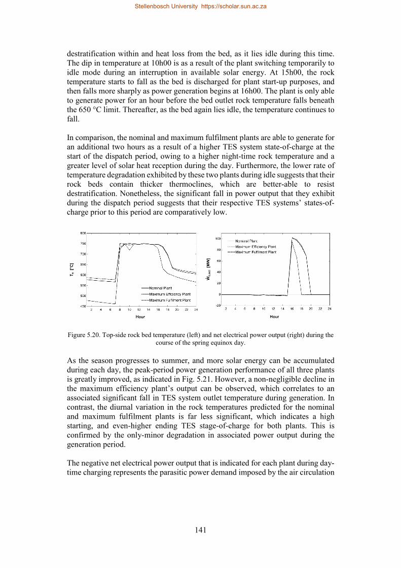
141

destratification within and heat loss from the bed, as it lies idle during this time. The dip in temperature at 10h00 is as a result of the plant switching temporarily to idle mode during an interruption in available solar energy. At 15h00, the rock temperature starts to fall as the bed is discharged for plant start-up purposes, and then falls more sharply as power generation begins at 16h00. The plant is only able to generate power for an hour before the bed outlet rock temperature falls beneath the 650 °C limit. Thereafter, as the bed again lies idle, the temperature continues to fall. In comparison, the nominal and maximum fulfilment plants are able to generate for an additional two hours as a result of a higher TES system state-of-charge at the start of the dispatch period, owing to a higher night-time rock temperature and a greater level of solar heat reception during the day. Furthermore, the lower rate of temperature degradation exhibited by these two plants during idle suggests that their rock beds contain thicker thermoclines, which are better-able to resist destratification. Nonetheless, the significant fall in power output that they exhibit during the dispatch period suggests that their respective TES systems’ states-of-charge prior to this period are comparatively low.

Figure 5.20. Top-side rock bed temperature (left) and net electrical power output (right) during the course of the spring equinox day.

As the season progresses to summer, and more solar energy can be accumulated during each day, the peak-period power generation performance of all three plants is greatly improved, as indicated in Fig. 5.21. However, a non-negligible decline in the maximum efficiency plant’s output can be observed, which correlates to an associated significant fall in TES system outlet temperature during generation. In contrast, the diurnal variation in the rock temperatures predicted for the nominal and maximum fulfilment plants is far less significant, which indicates a high starting, and even-higher ending TES stage-of-charge for both plants. This is confirmed by the only-minor degradation in associated power output during the generation period. The negative net electrical power output that is indicated for each plant during day-time charging represents the parasitic power demand imposed by the air circulation


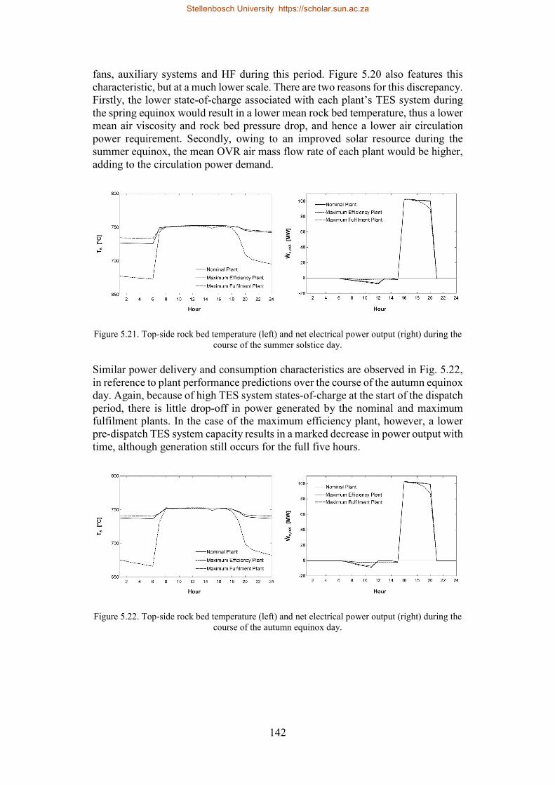
142

fans, auxiliary systems and HF during this period. Figure 5.20 also features this characteristic, but at a much lower scale. There are two reasons for this discrepancy. Firstly, the lower state-of-charge associated with each plant’s TES system during the spring equinox would result in a lower mean rock bed temperature, thus a lower mean air viscosity and rock bed pressure drop, and hence a lower air circulation power requirement. Secondly, owing to an improved solar resource during the summer equinox, the mean OVR air mass flow rate of each plant would be higher, adding to the circulation power demand.

Figure 5.21. Top-side rock bed temperature (left) and net electrical power output (right) during the course of the summer solstice day.

Similar power delivery and consumption characteristics are observed in Fig. 5.22, in reference to plant performance predictions over the course of the autumn equinox day. Again, because of high TES system states-of-charge at the start of the dispatch period, there is little drop-off in power generated by the nominal and maximum fulfilment plants. In the case of the maximum efficiency plant, however, a lower pre-dispatch TES system capacity results in a marked decrease in power output with time, although generation still occurs for the full five hours.

Figure 5.22. Top-side rock bed temperature (left) and net electrical power output (right) during the course of the autumn equinox day.


143

By mid-winter, as shown in Fig. 5.23, the limited solar resource results in lower pre-dispatch states-of-charge for all three plants’ TES systems, leading to a significant period of reduced-load operation of the nominal and maximum fulfilment plants, and deep part-load operation of the maximum efficiency plant. While the former plants are able to dispatch power for the full peak period, the latter plant is only able to generate for two of the five hours. This marked level of curtailment is explained by the dramatic fall in rock bed outlet temperature during the associated discharge period, which in turn is the result of the exit of a very thin thermocline from the bed. The reduced day-time parasitic power demand can be attributed to lower TES system capacities and a lower level of solar energy collection.

Figure 5.23. Top-side rock bed temperature (left) and net electrical power output (right) during the course of the winter solstice day.

5.6 Summary and Conclusion This study has sought to investigate the thermodynamic performance and operating characteristics of a large-scale OVR CSP plant, incorporating a rock bed TES system, and designed for peak-period power generation. The specific objectives of the work were to a) establish performance estimates for the technology when deployed in this operating role, and b) explore the relationship between plant performance, heliostat field size, and TES system capacity. For this purpose, a plant design tool was developed in the EES programming environment to facilitate the design of several test plants, designated to operate in Daggett, California, with a rated capacity of 100 MWe. The distinguishing feature of each test plant was its solar multiple fraction, with the nominal plant being assigned a solar multiple fraction of one, and five additional plants assigned solar multiple fractions of between 0.5 and 0.9. A plant design methodology was also proposed, in order to deal with design considerations specific to the plant technology.


144

A separate plant performance tool was developed to enable the quasi-steady performance of each plant over a year-long period to be simulated. This tool was based upon a coupled arrangement of detailed models of each of the constituent plant systems, namely the heliostat field, open volumetric receiver, air distribution network, thermal energy storage and power block systems. Plant performance was calculated on the basis of the sizing and design-point parameters set by the plant design tool, as well as hourly TMY3 data recorded for Daggett. Several key findings evolved from the performance data generated. Firstly, the annualised solar-electric efficiencies predicted for all plants considered were observed to be relatively poor, peaking at approximately 12.5 %. This was found to be as a consequence of the high parasitic power demand imposed by the air circulation and ACC fans of each plant. At face value, this observation suggests that the performance benefit derived from being able to operate the power block at a high live steam temperature, as a result of using air as a heat transfer fluid, is largely negated by the energy penalty associated with air circulation. Secondly, peak-period energy fulfilment was shown to exhibit a much greater dependency on plant solar multiple fraction than plant thermal storage capacity, as gauged by the associated rock bed height. For the plant configurations considered, energy fulfilment was indicated to vary between approximately 55 % and 95 %. Thirdly, annual solar-electric efficiency demonstrated an essentially inversely proportional relationship with annual energy yield. Achieving high efficiency requires a plant to feature a low solar multiple fraction and only moderate thermal storage capacity. This is demonstrated by the performance metrics of the plant found to offer the maximum efficiency, which exhibited an annual solar-electric efficiency of 12.6 %, but an energy fulfilment factor of only 69.1 %. An additional drawback of this configuration is that energy yield was shown to vary significantly from season to season. Conversely, the performance metrics of the plant able to achieve the greatest energy yield, suggested that achieving a high energy yield requires a plant to feature both a high solar multiple fraction and thermal storage capacity. This plant achieved an energy fulfilment factor of 94.2 %, but a solar-electric efficiency of only 10 %. The reduced efficiency was found to be the result of significant solar energy shedding during the summer months, and manifested despite the fact that the plant’s greater depth of thermal storage permitted power block operation at appreciably higher mean load levels. Ultimately, optimal CSP plant configurations are selected on the basis of levelised electricity cost minimisation, in the context of associated market pricing structures. Furthermore, certain performance characteristics may be imposed by regulatory requirements, such as minimum permissible electricity delivery levels, annually or even seasonally. Therefore, in order for comprehensive conclusions to be drawn regarding the economic competitiveness/viability of the CSP plant technology


145

studied here, a thorough thermoeconomic analysis and optimisation study is required. In particular, such a study should explore the impact of key technical plant parameters on electricity pricing. Appropriate parameters could include design-point meteorological conditions, heliostat field configuration settings, and certain characteristics of the air distribution system, such as design-point duct velocities, and of the power block, such as the number of air-cooled condenser units utilised. Attention should also be given to the selection of rock bed parameters, such as mean rock particle size, cut-off outlet temperatures, as well as design-point air mass flux. In conclusion, this study has, for the first time, evaluated the long-term performance characteristics of a large-scale OVR CSP plant incorporating rock bed thermal storage, while fulfilling a peaking duty. Based solely on thermodynamic performance predictions, the study has identified key behavioural trends and operating characteristics inherent to the technology.


146

6

Closure

6.1 Original Objectives

In response to clearly identified shortfalls in documented knowledge, this study has sought to develop a comprehensive understanding of the performance and operating characteristics of a large-scale OVR CSP plant incorporating rock bed TES and deployed as a means of generating peak-period electrical power. To achieve this aim, the following specific objectives were set:

1. Develop a comprehensive understanding of the research landscape associated with OVR CSP plant technology, with particular emphasis on plant and constituent system performance modelling activities.

2. Develop a computational tool capable of modelling the design-point performance of a large OVR CSP plant.

3. Develop a computationally-efficient rock bed TES system model. 4. Use outcomes of the above objectives to develop computational tools

capable of a) deriving detailed design parameters for and b) modelling the annual performance of a large-scale peaking OVR CSP plant employing rock bed TES.

5. Propose recommendations for future work based on the study’s findings.

The section that follows details the extent to which each of these objectives were met by describing the contributions arising from the study. 6.2 Contributions Objective 1 was addressed by means of the literature review presented in Chapter 2, which was published as an article in volume 82 of Renewable and Sustainable Energy Reviews. The review sought to identify and interrogate performance modelling studies associated with OVR CSP plant technology and published since the turn of the century. In particular, literature relating to fully-integrated OVR CSP plants, be they existing, proposed or conceptual, and elements of the technology still undergoing maturation, were of interest. The review identified sixty-three applicable studies associated with the period 2000-2016; fourteen concerning


147

receiver systems, twenty-two concerning packed bed TES, and twenty-seven concerning integrated plants. The review found that appreciable advancements have been made in the development of physically-representative and efficient performance models of constituent systems and integrated plants. These have clearly led to an improved understanding of operational characteristics, aided the development of control strategies, and provided a basic indication of how system and plant performance can be improved. However, comprehensive model validation has only rarely been demonstrated, with numerous studies providing no indication of validation whatsoever. This observation speaks to the lack of experimental performance data available to the research community. In addition, very few studies undertook formal optimisation exercises, and no studies were found to investigate the long-term performance of plants incorporating rock bed TES systems, or the performance of plants operating in a peaking role. Based on the review’s findings, several recommendations were made concerning future avenues of research. In a holistic sense, the review’s primary contribution was to frame the state of development in OVR CSP plant technology in the context of performance modelling activities, and to highlight existing knowledge gaps that such activities can assist in closing. On this basis, Objective 1 has been achieved. Objective 2 was addressed by means the study presented in Chapter 3, which was published as an article in volume 127 of Solar Energy. The study employed a custom-developed computational tool to investigate the thermodynamic interaction between the receiver and power block of a 100 MWe OVR CSP plant at the design point. Of particular interest was the impact that the selection of HRSG configuration and design parameters has on overall plant performance. In terms of validation, the power block system model used by the tool could be validated against published data, simulated for a similar OVR CSP plant by means of commercial software used for steady-state heat balance modelling. Although not explicitly validated, the OVR model was directly derived from published experimental data associated with a state-of-the-art OVR absorber module. In published literature, this data source appears to stand alone in terms of quality and detail. The basic model used to determine the design-point optical efficiency of the heliostat field was derived using published data simulated using a well-established code. A total of twelve plant configurations were designed, based on the consideration of three water/steam cycle pressure levels with or without reheating, two receiver air return strategies. The general performance characteristics of each configuration were presented, and associated best-performance operating points were identified. A significant variation in solar-electric efficiency was observed across the plant


148

range, highlighting a strong sensitivity to HRSG characteristics. With respect to the technology levels considered, the plant featuring a dual-pressure, reheated water/steam cycle with receiver air return exhibited the best solar-electric efficiency. The study also clearly demonstrated that the return of HRSG outlet air to the OVR was universally beneficial to solar-electric efficiency, irrespective of HRSG settings, and despite the additional parasitic power demand incurred. Furthermore, the sensitivity of plant performance to HRSG pinch-point temperature difference and deaerator outlet temperature was shown to be appreciable. The primary contribution of the study described in Chapter 3 was to quantify, for the first time in published literature, the significance of the thermodynamic interaction that exists between the receiver and water/steam cycle of a large-scale OVR CSP plant, and the impact that this interaction has on plant performance. This contribution was enabled by the development of a design-point performance modelling tool, which satisfies Objective 2. Objective 3 was addressed by means of the study presented in Chapter 4, which was published as an article in volume 17 of the Journal of Energy Storage. The work sought to assess the suitability of applying the local thermal equilibrium assumption as a means of improving the computational efficiency of rock bed TES models in the context of CSP plant operation. This assessment was made on the basis of a comparative performance evaluation of custom-formulated LTE and LTNE packed bed models employed in annual rock bed TES performance simulations. The validity of both rock bed models could be established using a combination of experimental data and published simulation data. Experimental data was used to validate the prediction of rock and air temperature profiles during the charging and discharging processes. Published simulation data was used to validate the prediction of bed pressure drop and bed thermal destratification during bed idle. No published data relating to the realistic long-term operation of CSP-based packed beds could be located by the author, so validation in this sense was not possible. The study detected an instability phenomenon in the numerical solution of the LTE model discretised by means of central differencing. The instability was found to be primarily sensitive to particle diameter and spatial discretisation resolution, and manifested in both single- and multi-cycle simulations. Key findings were also made in respect of spatial and temporal grid independence characteristics associated with such simulations. Concerning the correlation between the LTE and LTNE models, agreement was assessed in terms of annual exergy yield, generation time and rock bed blowing work, for parametric variations in bed charging temperature, discharge bed mass flux, rock particle diameter and rock type. Excellent inter-model correlation was observed with respect to exergy yield and generation time predictions across the


149

parameter spectrum, however significant discrepancies arose in the estimation of blowing work. These discrepancies could be directly attributed to variances in the prediction of bed thermocline behaviour. Regarding computational efficiency, it was shown that annual simulations could be greatly accelerated for both models by the coarsening of temporal and spatial discretisation resolution. Reducing temporal resolution while retaining fine spatial resolution resulted in significant improvements in computational efficiency without excessively compromising fidelity. The study concluded that while the LTE assumption presented a reasonable means of rock bed model simplification and resulted in significant reductions in computational overhead, the LTNE model proved to offer a more robust approach with similar levels of cost-efficiency when employing fine spatial and course temporal discretisation resolutions. The primary contribution of the study reported in Chapter 4 was to assess, for the first time in published literature, the value and fidelity implications of applying the LTE simplification in the prediction of long-term rock bed TES system performance. The study is seemingly the first of its kind concerning gas-solid packed bed CSP TES systems in general. Based on its findings, a validated, computationally-efficient rock bed TES system model was developed, satisfying Objective 3. Objective 4 was addressed by means of the study presented in Chapter 5 in the form of an unpublished manuscript due to be submitted shortly. The work employed custom-developed computational tools to firstly design a 100 MWe peaking OVR CSP plant with rock bed TES, as well as several related variants, and secondly model the operation of these plants over the course of a simulation year. The specific objectives of the work were to a) establish performance estimates for the technology when deployed in a peak power generation role, and b) explore the relationship between plant performance, plant solar multiple fraction, and TES system capacity. To this end, the performance of six plants was investigated, having solar multiple fractions ranging from 1 to 0.5. In terms of model validation, the plant design tool employed in the study was largely derived from the validated system models presented in Chapter 3. In this case, however, the well-established SolarPILOT research code was used for heliostat field design and performance prediction, and an ACC model based on published design data was incorporated. The plant performance tool incorporated off-design models of the HF, OVR, ADN and PB systems, as well as the validated LTNE rock bed model developed in the study presented in Chapter 4. Off-design HF performance was modelled on the basis of heliostat optical efficiency matrices generated by SolarPILOT. Off-design OVR performance was implicitly predicted by the receiver model used in the study


150

presented in Chapter 3. Off-design ADN performance was modelled on the basis published fan and VFD-motor performance data, although the uniqueness of the ADN system inhibited explicit system model validation. Off-design PB performance was captured on the basis of the off-design response of each of the PB system’s various component models, which were themselves based upon published modelling methodologies and/or design and performance data. A lack of detailed benchmark power block design parameters and performance data ultimately prevented the validation the PB system model in its entirety. Several key findings arose from the study. Firstly, the best-performing plant configuration exhibited a relatively poor annualised solar-electric efficiency relative to its design-point performance, with an efficiency of approximately 12.5 %. This was attributed to the high parasitic power demand imposed by each plant’s air circulation and ACC fans, and implies that the performance benefit derived from an elevated HTF temperature is largely negated by the energy penalty associated with HTF circulation. Secondly, peak-period energy fulfilment showed a much greater dependency on plant solar multiple fraction than plant thermal storage capacity. Across the plant range, a significant variation of energy fulfilment was indicated, with minimum and maximum values of approximately 55 % and 95 %. Thirdly, annual solar electric efficiency and annual energy yield were found to be inversely related. In this sense, achieving high efficiency requires a plant to feature a low solar multiple fraction – in order to avoid excessive solar shedding – and only moderate thermal storage capacity – in order to avoid an excessive pressure drop across the rock bed. Conversely, the achievement of a high energy yield requires a high solar multiple fraction and storage capacity, which contribute to a compromised solar-electric efficiency. Finally, an observation of hourly plant operating trends highlights the significant effect that rock bed thermocline exit during TES system discharge has on plant performance. The deterioration in plant power production was demonstrated to be appreciable for small decreases in rock bed air outlet temperature, and dramatic for large decreases. When in operation, rock bed thermocline stratification is greatly degraded by a variety of diffusive effects, resulting in earlier-than-desired thermocline exit and a sharp drop-off in power generation. This appears to be a problematic drawback of rock bed TES. This final passage of work served as the culmination of the overall study by drawing on the findings and resources generated during the previous studies. Its primary contribution was to evaluate, for the first time in published literature, the levels of performance that can be achieved by a large-scale OVR CSP plant incorporating rock bed TES and fulfilling a peaking duty, and to identify key behavioural trends and operating characteristics inherent to the technology. On this basis, Objective 4 has been satisfied.


151

6.3 Recommendations for Future Work With respect to Objective 5, this study provides the basis for several potential avenues of future work. First and foremost, the cost-competitiveness of the plant configurations considered in Chapter 5 should be evaluated. To achieve full value, such an analysis should be based upon the latest hardware cost estimates, and in the context of current energy market conditions. The resulting economic metrics should further be compared to those associated with competing CSP technologies. In addition, the performance and operating characteristics of a similar plant configuration, but serving baseload duty instead, should be evaluated in the same manner. The capacity to predict economic performance is a pre-requisite for plant optimisation exercises. Key subjects of such exercises would be the optimal selection of plant design-point specifications and system capacities, such as ACC capacity. The direct impact that thermocline degradation has on plant power output should be quantitatively assessed, and methods of mitigating this effect, over and above the use of phase change materials, should be explored. The cost and performance implications of using rock as opposed to engineered thermal media in OVR CSP plants should also be quantified. Furthermore, the fidelity implications of using one-dimensional models to predict packed bed TES system behaviour, as opposed to higher-dimension models, need to be determined. This is especially important in consideration of the sensitivity of plant output to TES system air outlet temperature demonstrated here. The development and implementation of a more detailed, multi-dimensional OVR system model, that is able to account for the local variation of absorber efficiency across the extent of the OVR, should be pursued. In addition, the performance-enhancing potential of several promising OVR absorber architectures that have recently been conceived should be investigated. Regarding receiver air re-entrainment, the impact of wind exposure on this phenomenon is very poorly understood and no relations appear to exist for the prediction thereof. Until suitable models can be derived for this purpose, major plant performance uncertainties will remain. Finally, an opportunity exists for photovoltaic arrays to be used to meet the daytime parasitic power demand of OVR CSP plants. This is in consideration of the significant level of synchronisation that would exist between air circulation fan demand and the power output of an augmenting photovoltaic array. Hybridisation of this nature would effectively improve the solar-electric efficiency of such a plant, and may well reduce the cost of electricity it generates.


152

References [1] IPCC. Climate Change 2014: Mitigation of Climate Change. New York:

Cambridge University Press; 2014.

[2] IRENA. Renewable Power Generation Costs in 2017. Abu Dhabi: International Renewable Energy Agency; 2018.

[3] IRENA. Electricity Storage and Renewables: Costs and Markets to 2030. Abu Dhabi: International Renewable Energy Agency; 2017.

[4] Denholm P, Mehos M. Enabling Greater Penetration of Solar Power via the Use of CSP with Thermal Energy Storage. Golden, CO: 2011.

[5] Turchi CS, Vidal J, Bauer M. Molten salt power towers operating at 600–650 °C: Salt selection and cost benefits. Sol Energy 2018;164:38–46. doi:10.1016/J.SOLENER.2018.01.063.

[6] Ho CK, Iverson BD. Review of high-temperature central receiver designs for concentrating solar power. Renew Sustain Energy Rev 2014;29:835–46. doi:10.1016/j.rser.2013.08.099.

[7] Fricker HW. Proposal for a novel type of solar gas receiver. Proc. Int. Semin. Sol. Therm. Heat Prod., 1983, p. 38–40.

[8] Hennecke K, Schwarzbözl P, Koll G. The solar tower Julich- A solar thermal power plant for test and demonstration of air receiver technology. Proc ISES World Congr 2007 Sol Energy Hum Settl 2007;Beijing, C:1749–53.

[9] EIA. California wholesale electricity prices are higher at the beginning and end of the day - Today in Energy - U.S. Energy Information Administration (EIA). Today in Energy 2017. https://www.eia.gov/todayinenergy/detail.php?id=32172 (accessed November 4, 2018).

[10] Pitot de la Beaujardiere JFP, Reuter HCR. A review of performance modelling studies associated with open volumetric receiver CSP plant technology. Renew Sustain Energy Rev 2017. doi:10.1016/j.rser.2017.10.086.

[11] Pitot de la Beaujardiere JFP, Reuter HCR, Klein SA, Reindl DT. Impact of HRSG characteristics on open volumetric receiver CSP plant performance. Sol Energy 2016;127. doi:10.1016/j.solener.2016.01.030.

[12] Pitot de la Beaujardiere J-FP, von Backström TW, Reuter HCR. Applicability of the Local Thermal Equilibrium Assumption in the Performance Modelling of CSP Rock Bed Thermal Energy Storage Systems.


153

J Energy Storage 2017.

[13] Pitot de la Beaujardiere J-FP, Allen KG, Reuter HCR, von Backström TW. The Suitability of the Infinite NTU Model for Long-Term Rock Bed Thermal Storage Performance Simulation. Proc. Third South. African Sol. Energy Conf., 2015, p. 549–54.

[14] Fricker HW. Study on the possibilities for a solar thermal power plant in the Val Maroz. Bull SEV/VSE 1985;76:558–62.

[15] Burgos JF. Design and optimization of a concentrated solar power plant using a volumetric receiver and a Kalina cycle. Masters Thesis, Technical University of Denmark, 2014.

[16] Zanganeh G, Khanna R, Walser C, Pedretti A, Haselbacher A, Steinfeld A. Experimental and numerical investigation of combined sensible-latent heat for thermal energy storage at 575°C and above. Sol Energy 2015;114:77–90. doi:10.1016/j.solener.2015.01.022.

[17] Tescari S, Breuer S, Roeb M, Sattler C, Flucht F, Schmücker M, et al. Design of a Thermochemical Storage System for Air-operated Solar Tower Power Plants. Energy Procedia 2015;69:1039–48. doi:10.1016/j.egypro.2015.03.203.

[18] Romero M, Buck R, Pacheco JE. An Update on Solar Central Receiver Systems, Projects, and Technologies. J Sol Energy Eng 2002;124:98. doi:10.1115/1.1467921.

[19] von Storch H, Stadler H, Roeb M, Hoffschmidt B. Efficiency potential of indirectly heated solar reforming with open volumetric solar receiver. Appl Therm Eng 2015;87:297–304. doi:10.1016/j.applthermaleng.2015.05.026.

[20] Roldán MI, Zarza E, Casas JL. Modelling and testing of a solar-receiver system applied to high-temperature processes. Renew Energy 2015;76:608–18. doi:10.1016/j.renene.2014.11.075.

[21] Hoffschmidt B. Vergleichende bewertung verschiedener konzepte volumetrischer strahlungsempfanger. D L R - Forschungsberichte 1997.

[22] Kribus A, Gray Y, Grijnevich M, Mittelman G, Mey-Cloutier S, Caliot C. The promise and challenge of solar volumetric absorbers. Sol Energy 2014;110:463–81. doi:10.1016/j.solener.2014.09.035.

[23] Coelho B, Oliveira A, Schwarzbözl P, Mendes A. Biomass and central receiver system (CRS) hybridization: Integration of syngas/biogas on the atmospheric air volumetric CRS heat recovery steam generator duct burner. Renew Energy 2015;75:665–74. doi:10.1016/j.renene.2014.10.054.

[24] Koll G, Sahraoui T, Hoffschmidt B, Khedim A, Pomp S, Schwarzbözl P, et


154

al. ALSOL: Solar Thermal Tower Power Plant Algeria. Proc. 17th SolarPACES Conf., Granada, Spain: 2011.

[25] Chavez JM, Chaza C. Testing of a porous ceramic absorber for a volumetric air receiver. Sol Energy Mater 1991;24:172–81. doi:10.1016/0165-1633(91)90057-R.

[26] Bai F. One dimensional thermal analysis of silicon carbide ceramic foam used for solar air receiver. Int J Therm Sci 2010;49:2400–4. doi:10.1016/j.ijthermalsci.2010.08.010.

[27] Zanganeh G, Pedretti A, Zavattoni S, Barbato M, Steinfeld A. Packed-bed thermal storage for concentrated solar power - Pilot-scale demonstration and industrial-scale design. Sol Energy 2012;86:3084–98. doi:10.1016/j.solener.2012.07.019.

[28] Avila-Marin AL. Volumetric receivers in Solar Thermal Power Plants with Central Receiver System technology: A review. Sol Energy 2011;85:891–910. doi:10.1016/j.solener.2011.02.002.

[29] Pitot de la Beaujardiere J-FP, Reuter HCR, Klein SA, Reindl DT. Impact of HRSG characteristics on open volumetric receiver CSP plant performance. Sol Energy 2016;127:159–74. doi:10.1016/j.solener.2016.01.030.

[30] Romero M, Marcos MJ, Osuna R, Fernández V. Design and Implementation plan of a 10 MW Solar Tower Power Plant Based on Volumetric-Air Technology in Seville (Spain). Proc Sol 2000 2000:89–98. doi:10.1007/s10617-005-1199-z.

[31] Becker M, Fend T, Hoffschmidt B, Pitz-Paal R, Reutter O, Stamatov V, et al. Theoretical and numerical investigation of flow stability in porous materials applied as volumetric solar receivers. Sol Energy 2006;80:1241–8. doi:10.1016/j.solener.2005.11.006.

[32] Marcos MJ, Romero M, Palero S. Analysis of air return alternatives for CRS-type open volumetric reciever. Energy 2004;29:677–86. doi:10.1016/S0360-5442(03)00176-2.

[33] Behar O, Khellaf A, Mohammedi K. A review of studies on central receiver solar thermal power plants. Renew Sustain Energy Rev 2013;23:12–39. doi:10.1016/j.rser.2013.02.017.

[34] Singh R, Saini RP, Saini JS. Models for predicting thermal performance of packed bed energy storage system for solar air heaters - A review. Open Fuels Energy Sci J 2009;2:47–53. doi:10.2174/1876973X00902010047.

[35] Singh H, Saini RP, Saini JS. A review on packed bed solar energy storage systems. Renew Sustain Energy Rev 2010;14:1059–69. doi:10.1016/j.rser.2009.10.022.


155

[36] Liu M, Steven Tay NH, Bell S, Belusko M, Jacob R, Will G, et al. Review on concentrating solar power plants and new developments in high temperature thermal energy storage technologies. Renew Sustain Energy Rev 2016;53:1411–32. doi:10.1016/j.rser.2015.09.026.

[37] Gomez-Garcia F, González-Aguilar J, Olalde G, Romero M. Thermal and hydrodynamic behavior of ceramic volumetric absorbers for central receiver solar power plants: A review. Renew Sustain Energy Rev 2016;57:648–58. doi:10.1016/j.rser.2015.12.106.

[38] Capuano R, Fend T, Schwarzbözl P, Smirnova O, Stadler H, Hoffschmidt B, et al. Numerical models of advanced ceramic absorbers for volumetric solar receivers. Renew Sustain Energy Rev 2016;58:656–65. doi:10.1016/j.rser.2015.12.068.

[39] Hoffschmidt B, Geimer K, Kaufhold O, Göttsche J, Bauer E, Bauer J. Innovative volumetric absorber structures for solar tower power plants. Proc. 15th SolarPACES Conf., Berlin: 2009.

[40] Wu Z, Caliot C, Flamant G, Wang Z. Coupled radiation and flow modeling in ceramic foam volumetric solar air receivers. Sol Energy 2011;85:2374–85. doi:10.1016/j.solener.2011.06.030.

[41] Wu Z, Caliot C, Bai F, Flamant G, Wang Z, Zhang J, et al. Experimental and numerical studies of the pressure drop in ceramic foams for volumetric solar receiver applications. Appl Energy 2010;87:504–13. doi:10.1016/j.apenergy.2009.08.009.

[42] Téllez FM. Thermal Performance Evaluation of the 200 kWth SolAir Volumetric Receiver. 2003.

[43] Hirsch T, Ahlbrink N, Gall J, Nolte V, Teixeira-Boura C, Andersson J. vICERP - Final technical report. 2011.

[44] Ahlbrink N, Alexopoulos S, Andersson J, Belhomme B, Boura C, Gall J, et al. vICERP – The Virtual Institute of Central Receiver Power Plants: Modeling and Simulation of an Open Volumetric Air Receiver Power Plant. In: Troch I, Breitenecker F, editors. Proc. 6th Vienna Conf. Math. Model., Vienna: ARGESIM / ASIM; 2009.

[45] Belhomme B, Pitz-Paal R, Schwarzbozl P, Ulmer S. A New Fast Ray Tracing Tool for High-Precision Simulation of Heliostat Fields. J Sol Energy Eng 2009;131:031002. doi:10.1115/1.3139139.

[46] Ahlbrink N, Belhomme B, Pitz-Paal R. Modeling and Simulation of a Solar Tower Power Plant with Open Volumetric Air Receiver. Proc 7th Model Conf Como, Italy, Sep 20-22, 2009 2009;49:685–93. doi:10.3384/ecp09430048.


156

[47] Ahlbrink N, Andersson J, Diehl M, Maldonado Quinto D, Pitz-Paal R. Optimized operation of an open volumetric air receiver. Proc. 16th SolarPACES Conf., Perpignan, France: 2010, p. 1–10.

[48] Ahlbrink N, Andersson J, Diehl M, Pitz-Paal R. Optimization of the Mass Flow Rate Distribution of an Open Volumetric Air Receiver. J Sol Energy Eng 2013;135:041003. doi:10.1115/1.4024245.

[49] Mahdi Z. Numerical investigation of constructive measures to reduce convective losses of solar thermal power plants. Masters Thesis, FH Aachen, 2014.

[50] Roldán MI, Fernández-Reche J, Ballestrín J. Computational fluid dynamics evaluation of the operating conditions for a volumetric receiver installed in a solar tower. Energy 2016;94:844–56. doi:10.1016/j.energy.2015.11.035.

[51] Hoffschmidt B, Tellez FM, Valverde A, Fernandez J, Fernandez V. Performance Evaluation of the 200-kWth HiTRec-II Open Volumetric Air Receiver. J Sol Energy Eng 2003;125:87. doi:10.1115/1.1530627.

[52] Buck R, Barth C, Eck M, Steinmann WD. Dual-receiver concept for solar towers. Sol Energy 2006;80:1249–54. doi:10.1016/j.solener.2005.03.014.

[53] Eck M, Buck R, Wittmann M. Dual Receiver Concept for Solar Towers up to 100 MW. J Sol Energy Eng Asme 2006;128:293–301. doi:10.1115/1.2210501.

[54] Heller L, Gauché P. Dual-pressure air receiver cycle for direct storage charging. Energy Procedia, vol. 49, 2014, p. 1400–9. doi:10.1016/j.egypro.2014.03.149.

[55] Palero S, Romero M, Castillo JL. Comparison of Experimental and Numerical Air Temperature Distributions Behind a Cylindrical Volumetric Solar Absorber Module. J Sol Energy Eng 2008;130:011011. doi:10.1115/1.2807046.

[56] Achenbach T, Göttsche J, Kaufhold O, Hoffschmidt B. Development of an edge module for open volumetric receiver for the use of the radiation at the receiver boundary region. Proc. 17th SolarPACES Conf., Granada, Spain: 2011.

[57] Fend T, Schwarzbözl P, Smirnova O, Schöllgen D, Jakob C. Numerical investigation of flow and heat transfer in a volumetric solar receiver. Renew Energy 2013;60:655–61. doi:10.1016/j.renene.2013.06.001.

[58] Roldán MI, Smirnova O, Fend T, Casas JL, Zarza E. Thermal analysis and design of a volumetric solar absorber depending on the porosity. Renew Energy 2014;62:116–28. doi:10.1016/j.renene.2013.06.043.


157

[59] Fricker HW. Regenerative thermal storage in atmospheric air system solar power plants. Energy 2004;29:871–81. doi:10.1016/S0360-5442(03)00192-0.

[60] Allen KG. Performance characteristics of packed bed thermal energy storage for solar thermal power plants. Masters Thesis, University of Stellenbosch, 2010.

[61] Allen KG. Rock bed thermal storage for concentrating solar power plants. Doctoral Thesis, University of Stellenbosch, 2014.

[62] Allen KG, Von Backström TW, Kröger DG. Packed rock bed thermal storage in power plants: Design considerations. Energy Procedia 2013;49:666–75. doi:10.1016/j.egypro.2014.03.072.

[63] Allen KG, von Backström TW, Kröger DG. Packed bed pressure drop dependence on particle shape, size distribution, packing arrangement and roughness. Powder Technol 2013;246:590–600. doi:10.1016/j.powtec.2013.06.022.

[64] Kröger DG. SUNSPOT – The Stellenbosch University Solar Power Thermodynamic Cycle 2011. http://blogs.sun.ac.za/sterg/files/2011/ 05/SUNSPOT-2.pdf.

[65] Hughes PJ. The Design and Predicted Performance of Arlington House. Masters Thesis, University of Wisconsin-Madison, 1975.

[66] Heller L. Investigation of the Thermal Storage System for a 5 MWel Concentrated Solar Power (CSP) Pilot Plant. Masters Thesis, TU Dresden, 2012.

[67] Heller L, Gauché P. Modeling of the rock bed thermal energy storage system of a combined cycle solar thermal power plant in South Africa. Sol Energy 2013;93:345–56. doi:10.1016/j.solener.2013.04.018.

[68] Zunft S, Hanel M, Kruger M, Dreißigacker V, Gohring F, Wahl E. Julich Solar Power Tower—Experimental Evaluation of the Storage Subsystem and Performance Calculation. J Sol Energy Eng 2011;133:031019. doi:10.1115/1.4004358.

[69] Dreißigacker V, Müller-Steinhagen H, Zunft S. Thermo-mechanical analysis of packed beds for large-scale storage of high temperature heat. Heat Mass Transf Und Stoffuebertragung 2010;46:1199–207. doi:10.1007/s00231-010-0684-5.

[70] Kronhardt V, Alexopoulos S, Reißel M, Sattler J, Hoffschmidt B, Hänel M, et al. High-temperature thermal storage system for solar tower power plants with open-volumetric air receiver simulation and energy balancing of a discretized model. Energy Procedia 2013;49:870–7.


158

doi:10.1016/j.egypro.2014.03.094.

[71] Kharchenko N V. Thermische solaranlagen: grundlagen, planung und auslegung. Springer; 2012.

[72] Kronhardt V, Alexopoulos S, Reißel M, Latzke M, Rendón C, Sattler J, et al. Simulation of Operational Management for the Solar Thermal Test and Demonstration Power Plant Jülich Using Optimized Control Strategies of the Storage System. Energy Procedia 2015;69:907–12. doi:10.1016/j.egypro.2015.03.172.

[73] Zunft S, Dreißigacker V, Hahn J, Kammel J. Flow Distribution Calculations in Regenerator-Type Heat Storage for Solar Tower Plants. Proc. 17th SolarPACES Conf., Granada, Spain: 2011.

[74] Hänchen M, Brückner S, Steinfeld A. High-temperature thermal storage using a packed bed of rocks - Heat transfer analysis and experimental validation. Appl Therm Eng 2011;31:1798–806. doi:10.1016/j.applthermaleng.2010.10.034.

[75] Zanganeh G, Pedretti A, Zavattoni SA, Barbato MC, Haselbacher A, Steinfeld A. Design of a 100 MWhth packed-bed thermal energy storage. Energy Procedia 2013;49:1071–7. doi:10.1016/j.egypro.2014.03.116.

[76] Kuravi S, Trahan J, Goswami Y, Jotshi C, Stefanakos E, Goel N. Investigation of a High-Temperature Packed-Bed Sensible Heat Thermal Energy Storage System With Large-Sized Elements. J Sol Energy Eng 2013;135:041008. doi:10.1115/1.4023969.

[77] Mumma SA, Marvin WC. A method of simulating the performance of a pebble bed thermal energy storage and recovery system. Am Soc Mech Eng Am Inst Chem Eng Heat Transf Conf St Louis, Mo, Aug 9-11, 1976, ASME 6 P 1976.

[78] Barton NG. Simulations of air-blown thermal storage in a rock bed. Appl Therm Eng 2013;55:43–50. doi:10.1016/j.applthermaleng.2013.03.002.

[79] Zavattoni SA, Barbato MC, Pedretti A, Zanganeh G, Steinfeld A. High temperature rock-bed TES system suitable for industrial-scale CSP plant - CFD analysis under charge/discharge cyclic conditions. Energy Procedia 2014;46:124–33. doi:10.1016/j.egypro.2014.01.165.

[80] Mertens N, Alobaid F, Frigge L, Epple B. Dynamic simulation of integrated rock-bed thermocline storage for concentrated solar power. Sol Energy 2014;110:830–42. doi:10.1016/j.solener.2014.10.021.

[81] Anderson R, Bates L, Johnson E, Morris JF. Packed bed thermal energy storage: A simplified experimentally validated model. J Energy Storage 2015;4:14–23. doi:10.1016/j.est.2015.08.007.


159

[82] Hughes PJ, Klein SA, Close DJ. Packed Bed Thermal Storage Models for Solar Air Heating and Cooling Systems. ASME J Heat Transf 1976;98:336–8.

[83] Schlipf D, Schicktanz P, Maier H, Schneider G. Using Sand and other Small Grained Materials as Heat Storage Medium in a Packed Bed HTTESS. Energy Procedia 2015;69:1029–38. doi:10.1016/j.egypro.2015.03.202.

[84] Avila-Marin AL, Tellez FM, Sanchez F. Lab-Scale Characterization of Heat Storage Solutions for Concentrated Solar Power With Open Volumetric Central Receiver Technologies. Proc. 18th SolarPACES Conf., Marrakech, Morocco: 2012.

[85] Avila-Marin AL, Alvarez-Lara M, Fernandez-Reche J. A regenerative heat storage system for central receiver technology working with atmospheric air. Energy Procedia 2013;49:705–14. doi:10.1016/j.egypro.2014.03.076.

[86] Zunft S, Hänel M, Krüger M, Dreißigacker V. A design study for regenerator-type heat storage in solar tower plants - Results and conclusions of the HOTSPOT project. Energy Procedia 2013;49:1088–96. doi:10.1016/j.egypro.2014.03.118.

[87] Goel N, Gonzalez-Aguilar J, Romero M, Steinfeld A, Stefanakos E, Goswami DY. CRISPTower - A solar power tower R&D initiative in India. Energy Procedia 2014;57:301–10. doi:10.1016/j.egypro.2014.10.035.

[88] Zanganeh G, Commerford M, Haselbacher A, Pedretti A, Steinfeld A. Stabilization of the outflow temperature of a packed-bed thermal energy storage by combining rocks with phase change materials. Appl Therm Eng 2014;70:316–20. doi:10.1016/j.applthermaleng.2014.05.020.

[89] Yebra LJ, Berenguel M, Dormido S, Romero M. Modelling and Simulation of Central Receiver Solar Thermal Power Plants. Model Conf 2005 2005;52:413–21.

[90] Álvarez JD, Guzmán JL, Yebra LJ, Berenguel M. Hybrid modeling of central receiver solar power plants. Simul Model Pract Theory 2009;17:664–79. doi:10.1016/j.simpat.2008.11.004.

[91] Alexopoulos S, Hoffschmidt B, Rau C. Simulation Results for a Hybridization Concept of a Small Solar Tower Power Plant. Proc. 16th SolarPACES Conf., Perpignan, France: 2010.

[92] Alexopoulos S, Hoffschmidt B, Rau C. Comparison of Steady-State and Transient Simulations for Solar Tower Power Plants With Open-Volumetric Receiver. Proc. 17th SolarPACES Conf., Granada, Spain: 2011.

[93] Alexopoulos S, Rau C, Hoffschmidt B, Latzke M, Sattler J. Development of a Transient Heat Recovery Steam Generator of the Solar Tower Power Plant


160

Juelich. Proc. 18th SolarPACES Conf., Marrakech, Morocco: 2012.

[94] Grasse W. PHOEBUS: international 30 MWe solar tower plant. Sol Energy Mater 1991;24:82–94. doi:10.1016/0165-1633(91)90050-U.

[95] Meinecke W, Cordes S, Merten I. PHOEBUS Technology Program Solar Air Receiver (TSA) – Final Report on Test Evaluation. DLR (MD-ET), Koln: 1994.

[96] Osuna R, Fernández V, Romero M, Blanco M. A 10MW solar tower power plant for southern Spain. Proc. 10th SolarPACES Int. Symp. ‘Solar Therm. 2000,’ Sydney: 2000.

[97] Ziolko C, Schmitz M, Sattler J, Khedim A, Hoffschmidt B. AlSol – The open volumetric receiver technology moves to Africa. Proc. 16th SolarPACES Conf., Perpignan, France: 2010.

[98] Rau C, Alexopoulos S, Breitbach G, Hoffschmidt B, Latzke M, Doerbeck T, et al. Transient Simulation for Hybrid Solar Tower Power Plant with Open-Volumetric Receiver in Algeria. Proc. 18th SolarPACES Conf., Marrakech, Morocco: 2012, p. 1–13.

[99] Gall J, Abel D, Ahlbrink N, Pitz-Paal R, Andersson J, Diehl M, et al. Optimized Control of Hot-Gas Cycle for Solar Thermal Power Plants. 7th Int Model Conf 2009:490–5. doi:10.3384/ecp09430053.

[100] Dersch J, Schwarzbozl P, Richert T. Annual Yield Analysis of Solar Tower Power Plants With GREENIUS. J Sol Energy Eng 2011;133:031017. doi:10.1115/1.4004355.

[101] Quaschning V, Ortmanns W, Kistner R, Geyer M. Greenius: A New Simulation Environment for Technical and Economical Analysis of Renewable Independent Power Projects. Sol Forum 2001 2001:413–8.

[102] Ertl FU. Exergoeconomic Analysis and Benchmark of a Solar Power Tower with Open Air Receiver Technology. Masters Thesis, KTH Royal Institute of Technology, 2012.

[103] Reddy VS, Kaushik SC, Tyagi SK. Exergetic analysis and economic evaluation of central tower receiver solar thermal power plant. Int J Energy Res 2014;38:1288–303. doi:10.1002/er.3138.

[104] Coelho B, Varga S, Oliveira A, Mendes A. Optimization of an atmospheric air volumetric central receiver system: Impact of solar multiple, storage capacity and control strategy. Renew Energy 2014;63:392–401. doi:10.1016/j.renene.2013.09.026.

[105] Schwarzbözl P. A TRNSYS Model Library for Solar Thermal Electric Components (STEC), Reference Manual, Release 3.0, DLR 2006.


161

[106] Yamani N, Khellaf A, Mohammedi K. Parametric Study of Tower Power Plant Performances for Its Implementation in Algeria. Prog. Clean Energy, Vol. 2, Cham: Springer International Publishing; 2015, p. 993–1003. doi:10.1007/978-3-319-17031-2_65.

[107] Ouali HAL, Merrouni AA, Moussaoui MA, Mezrhab A. Electricity yield analysis of a 50 MW solar tower plant under Moroccan climate. Proc 2015 Int Conf Electr Inf Technol ICEIT 2015 2015:252–6. doi:10.1109/EITech.2015.7162978.

[108] Alexopoulos S, Hoffschmidt B, Rau C, Sattler J. Choice of Solar Share of a Hybrid Power Plant of a Central Receiver System and a Biogas Plant in Dependency of the Geographical Latitude. Proc. World Renew. Energy Congr. 2011, Linköping, Sweden: 2011, p. 3710–7. doi:10.3384/ecp110573710.

[109] Coelho B, Schwarzbözl P, Oliveira A, Mendes A. Biomass and central receiver system (CRS) hybridization: Volumetric air CRS and integration of a biomass waste direct burning boiler on steam cycle. Sol Energy 2012;86:2912–22. doi:10.1016/j.solener.2012.06.009.

[110] Coelho B. Study of a hybrid concentrating solar power plant for Portuguese conditions. Doctoral Thesis, University of Porto, 2014.

[111] Rau C, Alexopoulos S, Breitbach G, Hoffschmidt B, Latzke M, Sattler J. Transient simulation of a solar-hybrid tower power plant with open volumetric receiver at the location Barstow. Energy Procedia 2013;49:1481–90. doi:10.1016/j.egypro.2014.03.157.

[112] Latzke M, Alexoupoulos S, Kronhardt V, Rendón C, Sattler J. Comparison of Potential Sites in China for Erecting a Hybrid Solar Tower Power Plant with Air Receiver. Energy Procedia 2015;69:1327–34. doi:10.1016/j.egypro.2015.03.142.

[113] Heller L, Hoffmann J. Comparison of Different Configurations of a Combined Cycle CSP Plant. Proc. 2nd SASEC Conf., Port Elizabeth, South Africa: 2014.

[114] Heller L, Hoffmann J. A Cost and Performance Evaluation of SUNDISC: A Dual-pressure Air Receiver Cycle. Energy Procedia 2015;69:1287–95. doi:10.1016/j.egypro.2015.03.153.

[115] Sanders Associates Inc. 1/4-Megawatt Solar Receiver. Final Report. DOE/SF/90506-1. 1979.

[116] Becker M, Sánchez-González M. Report of the Wire Pack Volumetric Receiver Tests Performed at the PSA in 1987–1988. 1989.

[117] Hellmuth TE. Experimental Characterization, Modeling and Optimum of a


162

Wire Mesh Solar Volutric Air Receiver. PhD Thesis, New Mexico State University, 1995.

[118] Téllez F, Romero M, Heller P, Valverde A, Dibowski G, Ulmer S. Thermal Performance of “SolAir 3000 kWth” Ceramic Volumetric Solar Receiver. 12th Int. Symp. Sol. Power Chem. Energy Syst., Oaxaca, Mexico: 2004.

[119] Fend T, Hoffschmidt B, Pitz-Paal R, Reutter O, Rietbrock P. Porous materials as open volumetric solar receivers: Experimental determination of thermophysical and heat transfer properties. Energy 2004;29:823–33. doi:10.1016/S0360-5442(03)00188-9.

[120] Fend T, Pitz-Paal R, Reutter O, Bauer J örg, Hoffschmidt B. Two novel high-porosity materials as volumetric receivers for concentrated solar radiation. Sol Energy Mater Sol Cells 2004;84:291–304. doi:10.1016/j.solmat.2004.01.039.

[121] Fricker HW. PHOEBUS Phase 1B Executive Summary, Report. CH 5232 Villigen-PSI: Paul Scherrer Institute. 1990.

[122] Haeger M. PHOEBUS Technology Programme: Solar Air Receiver (TSA). PSA Technical Report PSA-TR02/94. 1994.

[123] Klein SA. EES - Engineering Equation Solver. Version 9.486, F-Chart Software 2013.

[124] Kehlhofer R, Hannemann F, Stirnimann F, Rukes B. Combined-cycle gas steam turbine power plants. PennWell; 2009.

[125] Lemmon E, Jacobsen R. Thermodynamic properties of air and mixtures of nitrogen, argon, and oxygen from 60 to 2000 K at pressures to 2000 MPa. J Phys 2000.

[126] Wagner W, Pruß A. The IAPWS Formulation 1995 for the Thermodynamic Properties of Ordinary Water Substance for General and Scientific Use. J Phys Chem Ref Data 2002;31:387–535. doi:10.1063/1.1461829.

[127] Avila-Marin AL, Tellez Sufrategui FM. Sensitivity and Parametric Analysis for a Medium Size Central Receiver Solar Power Plant. Proc. 18th SolarPACES Conf., Marrakech, Morocco: 2012.

[128] Aicia-Ciemat-Solucar. WinDelsol 1.0 user’s guide. Version 1.0 2002.

[129] Kroger DG. Air-cooled heat exchangers and cooling towers : thermal-flow performance evaluation and design. Volume II. PennWell; 2004.

[130] Ganapathy V. Industrial boilers and heat recovery steam generators : design, applications, and calculations. Marcel Dekker; 2003.

[131] Siemens. Steam Turbines for CSP Plants - Technical Brochure. Erlangen,


163

Germany: 2010.

[132] Anderson B. Brayton-Cycle Baseload Power Tower CSP System. 2013. doi:10.2172/1166984.

[133] Good P, Zanganeh G, Ambrosetti G, Barbato MC, Pedretti A, Steinfeld A. Towards a commercial parabolic trough CSP system using air as heat transfer fluid. Energy Procedia 2013;49:381–5. doi:10.1016/j.egypro.2014.03.041.

[134] Durisch W, Frick E, Kesselring P. Heat storage in solar power plants using solid beds. Proc. Third Int. Work. Sol. Therm. Cent. Receiv. Syst., Konstanz: 1986.

[135] SOTEL Consortium. METAROZ Study on the Possibilities for a Solar-Thermal Power Plant in the MAROZ Valley (VAL MAROZ). Zurich-Municipal Utility. 1984.

[136] Meier A, Winkler C, Wuillemin D. Experiment for modelling high temperature rock bed storage. Sol Energy Mater 1991;24:255–64. doi:10.1016/0165-1633(91)90066-T.

[137] Schumann TEW. Heat transfer: a liquid flowing through a porous prism. Heat Transf 1929:405–16.

[138] Summers WA, Shah YT, Klinzing GE. Heat-transfer parameters for an annular packed bed. Ind Eng Chem Res 1989;28:611–8. doi:10.1021/ie00089a018.

[139] Adebiyi GA, Chenevert DJ. An Appraisal of One-Dimensional Analytical Models for the Packed Bed Thermal Storage Systems Utilizing Sensible Heat Storage Materials. J Energy Resour Technol 1996;118:44. doi:10.1115/1.2792692.

[140] Wakao, N. and Kaguei S. Heat and mass transfer in packed beds. New York: Gordon and Breach Science Publishers; 1983. doi:10.1002/aic.690290627.

[141] Balakrishnan AR, Pei DCT. Heat Transfer in Gas-Solid Packed Bed Systems. 2. The Conduction Mode. Ind Eng Chem Process Des Dev 1979;18:40–6. doi:10.1021/i260069a004.

[142] Kunii D, Smith JM. Heat transfer characteristics of porous rocks. AIChE J 1960;6:71–8. doi:10.1002/aic.690060115.

[143] Vortmeyer D, Schaefer RJ. Equivalence of one- and two-phase models for heat transfer processes in packed beds: one dimensional theory. Chem Eng Sci 1974;29:485–91. doi:10.1016/0009-2509(74)80059-X.

[144] Riaz M. Analytical solutions for single-and two-phase models of packed-bed thermal storage systems. J Heat Transfer 1977.


164

[145] Jefferson CP. Prediction of Breakthrough Curves in Packed Beds. AIChE J 1972;18:409.

[146] Wakao N, Kaguei S, Funazkri T. Effect of fluid dispersion coefficients on particle-to-fluid heat transfer coefficients in packed beds. Chem Eng Sci 1979;34:325–36. doi:10.1016/0009-2509(79)85064-2.

[147] Wakao, N. Kato K. Effective Thermal Conductivity of Packed Beds. J Chem Eng Japan 1969;2:24–33.

[148] Thermophysical Properties of Matter. IFI/Plenum. Purdue University; 1970.

[149] Hiep DD. Transient heat transfer in porous media. Master Thesis. U.S. Naval Postgraduate School. Monterey, California, 1965.

[150] Sousa E. Finite differences for the convection-diffusion equation : On stability and boundary conditions. PhD Thesis, Oxford University, 2001.

[151] VDI. VDI-Wärmeatlas. Berlin, Heidelberg: Springer Berlin Heidelberg; 2006. doi:10.1007/978-3-540-32218-4.

[152] Hirsch T, Ahlbrink N, Pitz-paal R, Boura CT, Hoffschmidt B, Gall J, et al. Dynamic Simulation of a Solar Tower System With Open Volumetric Receiver. Proc. 17th SolarPACES Conf., Granada, Spain: 2011.

[153] Zanganeh G, Pedretti A, Haselbacher A, Steinfeld A. Design of packed bed thermal energy storage systems for high-temperature industrial process heat. Appl Energy 2015;137:812–22. doi:10.1016/j.apenergy.2014.07.110.

[154] CPUC Sets New Time-of-Use Periods for SDG&E to Reflect Changing Energy Market, Press Release, California Public Utilities Commission; 2017.

[155] Wilcox S, Marion W. Users Manual for TMY3 Data Sets. National Renewable Energy Laboratory. Technical Report NREL/TP-581-43156. Golden, CO: 2008.

[156] National Renewable Energy Laboratory. System Advisor Model. Version 2017.9.5. Golden, CO. 2017.

[157] NREL. Integrated Layout and Optimization Tool for Solar Power Towers (SolarPilot) n.d. https://www.nrel.gov/csp/solarpilot.html.

[158] Duffie JA, Beckman WA. Solar engineering of thermal processes. Wiley; 2013.

[159] Spencer. Fourier Series Representation of the Position of the Sun. Search 1971;2.

[160] DLR. Greenius Manual. Version 4.1.0.1, DLR Solar Research 2015:1–121.


165

[161] Heller L. Development of a Dual-Pressure Air Receiver System for the SUNDISC Cycle. 2016.

[162] Howden Axial Fans ApS. VARIAX Axial Flow Fans n.d.

[163] Cory W. Fans and Ventilation. 2005. doi:10.1016/B978-0-08-044626-4.X5000-1.

[164] Weber WJ, Cuzner RM, Ruckstadter E, Smith J. Engineering Fundamentals of Multi-MW Variable Frequency Drives — How They Work, Basic Types, and Application Considerations. Proc. 31st Turbomach. Symp., 2002, p. 177–94.

[165] Stodola A, Loewenstein LC. Steam and Gas Turbines. Volume 1. New York: McGraw-Hill Book Company; 1945.

[166] Xiang W, Chen Y. Performance improvement of combined cycle power plant based on the optimization of the bottom cycle and heat recuperation. J Therm Sci 2007;16:84–9. doi:10.1007/s11630-007-0084-4.

[167] Jüdes M, Vigerske S, Tsatsaronis G. Optimization of the Design and Partial-Load Operation of Power Plants Using Mixed-Integer Nonlinear Programming. Optim. Energy Ind., Springer-Verlag; 2009, p. 193–220.

[168] SOFBID. EBSILON Professional. http://www.sofbid.com n.d.

[169] Siemens AG. Steam turbines for CSP plants. 2011.

[170] Patnode A. Simulation and performance evaluation of parabolic trough solar power plants. 2006.

[171] Conradie AE, Kröger DG. Performance evaluation of dry-cooling systems for power plant applications. Appl Therm Eng 1996;16:219–32. doi:10.1016/1359-4311(95)00068-2.

[172] Shah RK, Sekulic DP. Fundamentals of heat exchanger design. John Wiley & Sons; 2003.

[173] ESDU. High-fin staggered tube banks: heat transfer and pressure drop for turbulent single phase gas flow. ESDU data item no. 86022. Engineering Science Data Unit International Ltd. London: 2005.

[174] Zhang G, Zheng J, Yang Y, Liu W. Thermodynamic performance simulation and concise formulas for triple-pressure reheat HRSG of gas-steam combined cycle under off-design condition. Energy Convers Manag 2016;122:372–85. doi:10.1016/j.enconman.2016.05.088.

[175] Ganapathy V. Simplify heat recovery steam generator evaluation. Hydrocarb Process 1990;69:3:77–82.


166

[176] Ganapathy V. Steam Generators and Waste Heat Boilers For Process and Plant Engineers. CRC Press; 2014.

[177] Costa AN, Vinicius M, Neves S, Cruz ME, Vieira LS. Maximum Profit Cogeneration Plant – MPCP: System Modeling, Optimization Problem Formulation, and Solution n.d.

[178] Wu X. Parameter optimization and performance analysis on large-scale combined-cycle cogeneration systems. Masters Thesis, Tsinghua University, 2005.

[179] ABB Incorporated. Energy Efficient Design of Auxiliary Systems in Fossil-Fuel Power Plants. 2009.

[180] ROCKWOOL Group. ProRox QM 970 Technical Data Sheet. 2013.

[181] Pitot de la Beaujardiere J-FP, von Backström TW, Reuter HCR. Applicability of the local thermal equilibrium assumption in the performance modelling of CSP plant rock bed thermal energy storage systems. J Energy Storage 2018;15. doi:10.1016/j.est.2017.09.003.


A.1

Appendix A: Chapter 2 Supporting Material Performance Modelling Study Details Tables A.1-A.3, that provide further details concerning the studies reviewed in Chapter 2, can be found on the proceeding pages.


A.2

Table A.1. Details associated with receiver system performance modelling studies.

Study Implementation

Softwarea System/s Considered

Modelling Sophisticationb

Modelling Scope

Temporal Regimec

Spatial Regimec Validation Demonstratedd

Abs

orbe

r Mod

ule

Subr

ecei

ver

Rec

eive

r

Sim

ple

Mod

erat

e

Com

plex

Ther

mal

Flui

d

Opt

imisa

tion

Stea

dy

Tran

sient

0D

1D

2D

3D

Yes

No

1. Marcos et al. [32] Fluent • • • • • • • 2. Ahlbrink et al. [44] Dymola • • • • • • • • 3. Ahlbrink et al. [46] Dymola • • • • • • • • 4. Ahlbrink et al. [47] C++ • • • • • • • • • 5. Ahlbrink et al. [48] C++ • • • • • • • • • 6. Mahdi [49] OpenFoam • • • • • 7. Roldán et al. [50] Fluent • • • • • • • 8. Buck et al. [52] - • • • • • • 9. Eck et al. [53] - • • • • • • 10. Heller and Gauché [54]

MATLAB • • • • • •

11. Palero et al. [55] Fluent • • • • • • • 12. Achenbach et al. [56] ANSYS (Multiphysics) • • • • • • • 13. Fend et al. [57] COMSOL • • • • • • • 14. Roldán et al. [58] Fluent • • • • • • • Number of Studies 4 5 8 2 6 6 13 11 3 11 3 1 1 7 4 5 9

Notes: aWith reference to the as-stated software used for receiver modelling specifically. bQualitative index assigned according to the judgement of the present authors. cWith specific regard to the receiver modelling component of the study. d“Yes” if model validation is demonstrated in-text, “No” if model validation has been demonstrated in prior works, or if model validation has not been undertaken. A dash indicates that no particular information was provided.



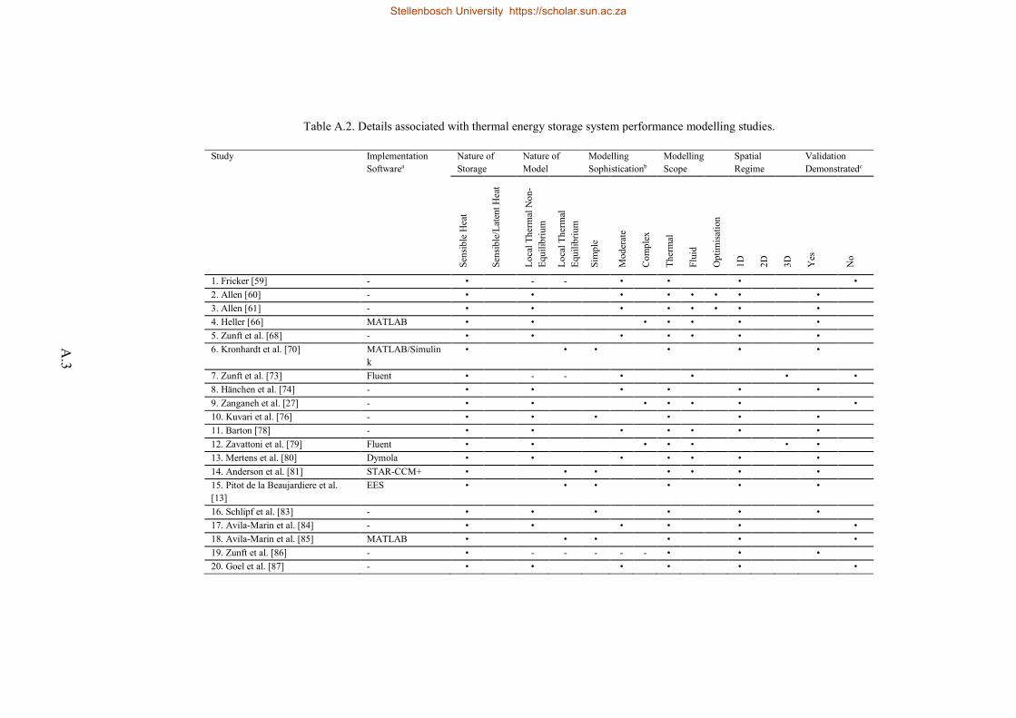
A.3

Table A.2. Details associated with thermal energy storage system performance modelling studies.

Study Implementation Softwarea

Nature of Storage

Nature of Model


Modelling Scope

Spatial Regime

Validation Demonstratedc

Sens

ible

Hea

t

Sens

ible

/Lat

ent H

eat

Loca

l The

rmal

Non

-Eq

uilib

rium

Loca

l The

rmal

Eq

uilib

rium

Sim

ple

Mod

erat

e

Com

plex

Ther

mal

Flui

d

Opt

imisa

tion

1D

2D

3D

Yes

No

1. Fricker [59] - • - - • • • • 2. Allen [60] - • • • • • • • • 3. Allen [61] - • • • • • • • • 4. Heller [66] MATLAB • • • • • • • 5. Zunft et al. [68] - • • • • • • • 6. Kronhardt et al. [70] MATLAB/Simulin

k • • • • • •

7. Zunft et al. [73] Fluent • - - • • • • 8. Hänchen et al. [74] - • • • • • • 9. Zanganeh et al. [27] - • • • • • • • 10. Kuvari et al. [76] - • • • • • • 11. Barton [78] - • • • • • • • 12. Zavattoni et al. [79] Fluent • • • • • • • 13. Mertens et al. [80] Dymola • • • • • • • 14. Anderson et al. [81] STAR-CCM+ • • • • • • • 15. Pitot de la Beaujardiere et al. [13]

EES • • • • • •

16. Schlipf et al. [83] - • • • • • • 17. Avila-Marin et al. [84] - • • • • • • 18. Avila-Marin et al. [85] MATLAB • • • • • • 19. Zunft et al. [86] - • - - - - - • • • 20. Goel et al. [87] - • • • • • •



A.4

Table A.2 (continued). Details associated with thermal energy storage system performance modelling studies.

Study Implementation Softwarea

Nature of Storage

Nature of Model


Modelling Scope

Spatial Regime

Validation Demonstratedc

Sens

ible

Hea

t

Sens

ible

/Lat

ent H

eat

Loca

l The

rmal

Non

-Eq

uilib

rium

Loca

l The

rmal

Eq

uilib

rium

Sim

ple

Mod

erat

e

Com

plex

Ther

mal

Flui

d

Opt

imisa

tion

1D

2D

3D

Yes

No

21. Zanganeh et al. [88] - • • • • • • 22. Zanganeh et al. [16] - • • • • • • Number of Studies 20 2 15 4 6 10 5 21 10 2 20 0 2 16 6

Notes: a) with reference to the as-stated software used for packed modelling specifically, b) a qualitative index assigned according to the judgement of the present authors, c) “Yes” if model validation is demonstrated in-text, “No” if model validation has been demonstrated in prior works, or if model validation has not been undertaken. A dash indicates that no particular information was provided.



A.5

Table A.3. Details associated with plant performance modelling studies.

Study Implementation Software Plant Type Operating Regime

Modelling Sophisticationa

Modelling Scope Temporal Regime

Validation Demonstratedb

Sola

r Fie

ld

Rec

eive

r

Stor

age

Pow

er B

lock

Esta

blish

ed P

lant

Prop

osed

Pla

nt

Con

cept

ual P

lant

Sola

r-Onl

y

Hyb

ridis

ed

Sim

ple

Mod

erat

e

Com

plex

Des

ign-

Poin

t Per

form

ance

Shor

t-Ter

m P

erfo

rman

ce

Ann

ual P

erfo

rman

ce

Opt

imisa

tion

Stea

dy

Tran

sient

Yes

No

1. Yebra et al. [89] - Dymola Dymola Dymola • • • • • • • 2. Álvarez et al. [90] - MATLAB MATLAB MATLAB • • • • • • • 3. Alexopoulos et al. [91] MATLAB MATLAB MATLAB MATLAB • • • • • • • 4. Alexopoulos et al. [92] MATLAB MATLAB MATLAB MATLAB • • • • • • • 5. Alexopoulos et al. [93] MATLAB MATLAB MATLAB MATLAB • • • • • • • 6. Romero et al. [30] DELSOL SOLERGY SOLERGY SOLERGY • • • • • • • 7. Koll et al. [24] - - - - • • - - - • • • • 8. Rau et al. [98] - MATLAB MATLAB MATLAB • • • • • • • 9. Gall et al. [99] STRAL Dymola Dymola Dymola • • • • • • • 10. Dersch et al. [100] GREENIUS GREENIUS GREENIUS GREENIUS • • • • • • • 11. Ertl [102] HFLCAL EES EBSILON EBSILON • • • • • • • 12. Reddy et al. [103] MATLAB - - EES • • • • • • • 13. Coelho et al. [104] HFLCAL EBSILON EBSILON • • • • • • • 14. Yamani et al. [106] TRNSYS TRNSYS TRNSYS TRNSYS • • • • • • • 15. Ouali et al. [107] GREENIUS GREENIUS GREENIUS GREENIUS • • • • • • • 16. Pitot de la Beaujardiere and Reuter [29]

EES EES • • • • • •

17. Alexopoulos et al. [108] MATLAB MATLAB MATLAB MATLAB • • • • • • • 18. Coelho et al. [109] HFLCAL EBSILON EBSILON • • • • • • • 19. Coelho et al. [23] HFLCAL EBSILON - EBSILON • • • • • • • 20. Rau et al. [111] MATLAB MATLAB MATLAB MATLAB • • • • • • • •



A.6

Table A.3 (continued). Details associated with plant performance modelling studies.

Study Implementation Software Plant Type Operating Regime

Modelling Sophisticationa

Modelling Scope Temporal Regime

Validation Demonstratedb

Sola

r Fie

ld

Rec

eive

r

Stor

age

Pow

er B

lock

Esta

blish

ed P

lant

Prop

osed

Pla

nt

Con

cept

ual P

lant

Sola

r-Onl

y

Hyb

ridis

ed

Sim

ple

Mod

erat

e

Com

plex

Des

ign-

Poin

t Per

form

ance

Shor

t-Ter

m P

erfo

rman

ce

Ann

ual P

erfo

rman

ce

Opt

imisa

tion

Stea

dy

Tran

sient

Yes

No

21. Latzke et al. [112] MATLAB MATLAB MATLAB • • • • • • • • 22. Buck et al. [52] HFCAL - IPSEpro • • • • • • • 23. Eck et al. [53] HFCAL - IPSEpro • • • • • • • 24. Burgos [15] MATLAB MATLAB MATLAB MATLAB • • • • • • • • 25. Heller and Gauché [54] MATLAB MATLAB MATLAB • • • • • • 26. Heller and Hoffman [113] MATLAB MATLAB MATLAB • • • • • • 27. Heller and Hoffmann [114] MATLAB MATLAB MATLAB • • • • • • Number of Studies 5 3 19 17 11 0 15 11 12 7 21 1 27 11 7 20

Notes: a) a qualitative index assigned according to the judgement of the present authors, b) “Yes” if model validation is demonstrated in-text, “No” if model validation has been demonstrated in prior works, or if model validation has not been undertaken. A dash indicates that no particular information was provided.



B.1

Appendix B: Chapter 3 Supporting Material

Power Block Process Flow Diagrams The process flow diagrams shown in Figs. B.1-B.3 illustrate the basic power block layout for the reheated single, dual and triple pressure plant configurations considered in the Chapter 3 study.

Figure B.1. Power block process flow diagram for the reheated single pressure plant configuration.

Figure B.2. Power block process flow diagram for the reheated dual pressure plant configuration.


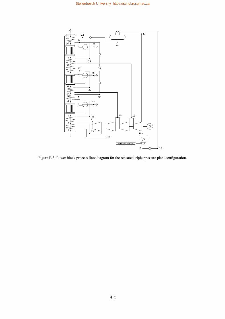
B.2

Figure B.3. Power block process flow diagram for the reheated triple pressure plant configuration.


C.1

Appendix C: Chapter 5 Supporting Material

C.1 Non-Default SolarPILOT Heliostat Field Model Parameters

for the Nominal Plant Design Table C.1 provides a listing of all non-default parameters applied in the SolarPILOT software when deriving the performance parameters of the nominal heliostat field design considered in Chapter 5. All other parameters required by the software were left at their default values.

Table C.1. Non-default SolarPILOT model parameters for the nominal plant heliostat field design.

Menu Option Sub-Option Parameter Value Climate Choose

Climate/Location Location CA Daggett.tm2

Plant Plant Sizing Solar Multiple 1 Layout Setup Design Point

Definition Heliostat Selection Criteria

Total Efficiency

Design Values Solar Field Design Power

370 MWth

Design-Point DNI Value

892 W/m2

Sun Position at Design Point

Summer Solstice

Field Configuration Tower Optical Height 201 m Receivers Receiver Geometry Receiver Height 18.7 m Receiver Diameter 15.6 m Optical Properties Receiver Thermal

Absorptance 1.00

Thermal Losses Design Point Receiver Thermal

0 kW/m2

Receiver Piping Loss Coefficient

0 kW/m

Performance Simulation

Sun Position Direct Normal Irradiation

892 W/m2

Month of the Year 6 Day of Month 20

The Solar Field Design Power parameter, which is used to size the heliostat field, is not equivalent to the quantity of radiation that must be intercepted by the OVR, ��𝑄𝑖𝑖𝑛𝑛𝑛𝑛. Therefore, in order for the field design to provide the OVR with the desired ��𝑄𝑖𝑖𝑛𝑛𝑛𝑛 value, this parameter was iteratively varied until the correct value is obtained. In addition, although SolarPILOT has the capability to approximate receiver and HTF distribution system thermal losses, this capability was not required as the plant design model accounted for these losses separately.


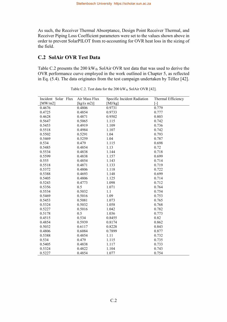
C.2

As such, the Receiver Thermal Absorptance, Design Point Receiver Thermal, and Receiver Piping Loss Coefficient parameters were set to the values shown above in order to prevent SolarPILOT from re-accounting for OVR heat loss in the sizing of the field. C.2 SolAir OVR Test Data Table C.2 presents the 200 kWth SolAir OVR test data that was used to derive the OVR performance curve employed in the work outlined in Chapter 5, as reflected in Eq. (5.4). The data originates from the test campaign undertaken by Téllez [42].

Table C.2. Test data for the 200 kWth SolAir OVR [42].

Incident Solar Flux [MW/m2]

Air Mass Flux [kg/(s m2)]

Specific Incident Radiation [MJ/kg]

Thermal Efficiency [-]

0.4676 0.4806 0.9731 0.779 0.4725 0.4854 0.9733 0.777 0.4628 0.4871 0.9502 0.803 0.5647 0.5065 1.115 0.742 0.5453 0.4919 1.109 0.736 0.5518 0.4984 1.107 0.742 0.5502 0.5291 1.04 0.793 0.5469 0.5259 1.04 0.787 0.534 0.479 1.115 0.698 0.5485 0.4854 1.13 0.72 0.5534 0.4838 1.144 0.718 0.5599 0.4838 1.157 0.699 0.555 0.4854 1.143 0.714 0.5518 0.4871 1.133 0.719 0.5372 0.4806 1.118 0.722 0.5388 0.4693 1.148 0.699 0.5405 0.4806 1.125 0.714 0.5243 0.4773 1.098 0.712 0.5356 0.5 1.071 0.764 0.5534 0.5032 1.1 0.754 0.5469 0.5016 1.09 0.753 0.5453 0.5081 1.073 0.765 0.5324 0.5032 1.058 0.768 0.5227 0.5016 1.042 0.782 0.5178 0.5 1.036 0.773 0.4515 0.534 0.8455 0.82 0.4854 0.5939 0.8174 0.862 0.5032 0.6117 0.8228 0.843 0.4806 0.6084 0.7899 0.877 0.5388 0.4854 1.11 0.732 0.534 0.479 1.115 0.735 0.5405 0.4838 1.117 0.733 0.5324 0.4822 1.104 0.743 0.5227 0.4854 1.077 0.754


C.3

Table C.2 (continued). Test data for the 200 kWth SolAir OVR [42].

Incident Solar Flux [MW/m2]

Air Mass Flux [kg/(s m2)]

Specific Incident Radiation [MJ/kg]

Thermal Efficiency [-]

0.5081 0.4757 1.068 0.755 0.4191 0.4693 0.8931 0.804 0.4466 0.4693 0.9517 0.785 0.4239 0.4741 0.8942 0.846 0.4304 0.4693 0.9172 0.796 0.4061 0.4628 0.8776 0.813 0.4126 0.4725 0.8733 0.823 0.3641 0.4693 0.7759 0.837 0.3382 0.4515 0.7491 0.846 0.5227 0.479 1.091 0.731 0.5372 0.4806 1.118 0.719 0.5372 0.479 1.122 0.718 0.5307 0.479 1.108 0.73 0.5243 0.4741 1.106 0.731 0.5162 0.479 1.078 0.743 0.5113 0.4757 1.075 0.746 0.5081 0.4757 1.068 0.757

C.3 Reference ACC Unit Design Parameters Table C.3 presents key design parameters of the reference ACC unit considered in Chapter 5, obtained from the work of Conradie and Kröger [171]. These parameters were used in the solution of Eqs. (5.39)-(5.41).

Table C.3. Design parameters of the reference ACC unit.

Parameter Value Fin outer diameter, 𝐷𝐷𝑓𝑓𝑖𝑖𝑛𝑛 [mm] 69.9 Tube outer diameter, 𝐷𝐷𝑛𝑛𝑑𝑑𝑎𝑎,𝑜𝑜 [mm] 38.1 Fin thickness, 𝑡𝑡𝑓𝑓𝑖𝑖𝑛𝑛 [mm] 0.35 Fin pitch (first row), 𝑝𝑝𝑓𝑓𝑖𝑖𝑛𝑛 [mm] 3.63 Thermal conductivity of fin material, 𝑘𝑘𝑓𝑓𝑖𝑖𝑛𝑛 [W/(m K)] 204 Tube transverse pitch, 𝑝𝑝𝑛𝑛𝑟𝑟𝑎𝑎 [mm] 76.2 Tube length, 𝐿𝐿𝑛𝑛𝑑𝑑𝑎𝑎 [m] 10 Number of tubes (first row), 𝑛𝑛𝑛𝑛𝑑𝑑𝑎𝑎 [-] 152

C.4 Heliostat Field Optical Efficiency Matrix for the Nominal

Plant Design Table C.4 presents discrete values of optical efficiency for the nominal plant design heliostat field, for various combinations of solar azimuth and elevation angles, as evaluated by the associated SolarPILOT model. An azimuth angle of 0° corresponds to due south.


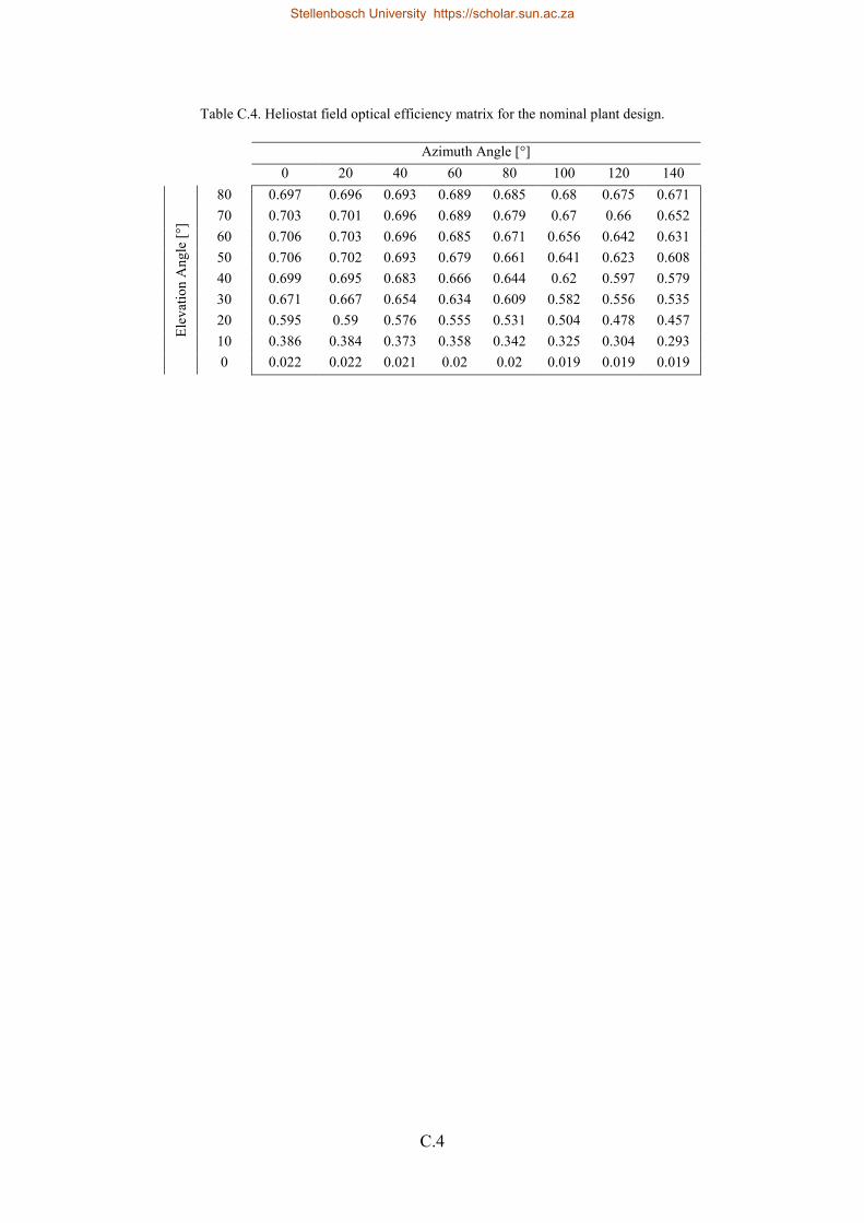
C.4

Table C.4. Heliostat field optical efficiency matrix for the nominal plant design.

Azimuth Angle [°] 0 20 40 60 80 100 120 140

Elev

atio

n A

ngle

[°]

80 0.697 0.696 0.693 0.689 0.685 0.68 0.675 0.671 70 0.703 0.701 0.696 0.689 0.679 0.67 0.66 0.652 60 0.706 0.703 0.696 0.685 0.671 0.656 0.642 0.631 50 0.706 0.702 0.693 0.679 0.661 0.641 0.623 0.608 40 0.699 0.695 0.683 0.666 0.644 0.62 0.597 0.579 30 0.671 0.667 0.654 0.634 0.609 0.582 0.556 0.535 20 0.595 0.59 0.576 0.555 0.531 0.504 0.478 0.457 10 0.386 0.384 0.373 0.358 0.342 0.325 0.304 0.293 0 0.022 0.022 0.021 0.02 0.02 0.019 0.019 0.019


performance modelling of an open volumetric receiver csp

Documents