performance guide for hpc applications on idataplex rel 1.0.2.pdf
TRANSCRIPT
Performance Guide for HPC Applications on iDataPlex dx360 M4 systems
A Performance Guide For HPC Applications
On the IBM® System x® iDataPlex® dx360® M4 System
Release 1.0.2 June 19, 2012
IBM Systems and Technology Group
Copyright ©2012 IBM Corporation
Page 1 of 153

Performance Guide for HPC Applications on iDataPlex dx360 M4 systems
Contents
Contributors...................................................................................................... 8
Introduction...................................................................................................... 9
1 iDataPlex dx360 M4 ................................................................................. 11 1.1 Processor .....................................................................................................11
1.1.1 Supported Processor Models ................................................................................. 12 1.1.2 Turbo Boost 2.0 ...................................................................................................... 13
1.2 System .........................................................................................................16 1.2.1 I/O and Locality Considerations.............................................................................. 17 1.2.2 Memory Subsystem................................................................................................ 17 1.2.3 UEFI......................................................................................................................... 20
1.3 Mellanox InfiniBand Interconnect ................................................................23 1.3.1 References .............................................................................................................. 27
2 Performance Optimization on the CPU ..................................................... 28 2.1 Compilers.....................................................................................................28
2.1.1 GNU compiler ......................................................................................................... 28 2.1.2 Intel Compiler ......................................................................................................... 29 2.1.3 Recommended compiler options ........................................................................... 29 2.1.4 Alternatives............................................................................................................. 46
2.2 Libraries .......................................................................................................47 2.2.1 Intel® Math Kernel Library (MKL) ........................................................................... 47 2.2.2 Alternative Libraries ............................................................................................... 48
2.3 References ...................................................................................................49
3 Linux......................................................................................................... 51 3.1 Core Frequency Modes.................................................................................51 3.2 Memory Page Sizes ......................................................................................51 3.3 Memory Affinity...........................................................................................52
3.3.1 Introduction............................................................................................................ 52 3.3.2 Using numactl ......................................................................................................... 52
3.4 Process and Thread Binding .........................................................................53 3.4.1 taskset..................................................................................................................... 53 3.4.2 numactl................................................................................................................... 54 3.4.3 Environment Variables for OpenMP Threads......................................................... 55 3.4.4 LoadLeveler............................................................................................................. 56
3.5 Hyper-Threading (HT) Management .............................................................57 3.6 Hardware Prefetch Control...........................................................................57 3.7 Monitoring Tools for Linux ...........................................................................58
3.7.1 Top.......................................................................................................................... 58 3.7.2 vmstat ..................................................................................................................... 59 3.7.3 iostat....................................................................................................................... 59 3.7.4 mpstat..................................................................................................................... 59
Copyright ©2012 IBM Corporation
Page 2 of 153
Performance Guide for HPC Applications on iDataPlex dx360 M4 systems
4 MPI........................................................................................................... 61 4.1 Intel MPI ......................................................................................................61
4.1.1 Compiling................................................................................................................ 61 4.1.2 Running Parallel Applications ................................................................................. 62 4.1.3 Processor Binding ................................................................................................... 63
4.2 IBM Parallel Environment ............................................................................64 4.2.1 Building an MPI program........................................................................................ 64 4.2.2 Selecting MPICH2 libraries...................................................................................... 65 4.2.3 Optimizing for Short Messages............................................................................... 65 4.2.4 Optimizing for Intranode Communications ............................................................ 65 4.2.5 Optimizing for Large Messages............................................................................... 65 4.2.6 Optimizing for Intermediate-Size Messages........................................................... 66 4.2.7 Optimizing for Memory Usage ............................................................................... 66 4.2.8 Collective Offload in MPICH2.................................................................................. 66 4.2.9 MPICH2 and PEMPI Environment Variables ........................................................... 67 4.2.10 IBM PE Standalone POE Affinity ............................................................................. 69 4.2.11 OpenMP Support .................................................................................................... 70
4.3 Using LoadLeveler with IBM PE ....................................................................70 4.3.1 Requesting Island Topology for a LoadLeveler Job................................................. 70 4.3.2 How to run OpenMPI and INTEL MPI jobs with LoadLeveler ................................. 71 4.3.3 LoadLeveler JCF (Job Command File) Affinity Settings ........................................... 71 4.3.4 Affinity Support in LoadLeveler .............................................................................. 72
5 Performance Analysis Tools on Linux ........................................................ 73 5.1 Runtime Environment Control......................................................................73
5.1.1 Ulimit ...................................................................................................................... 73 5.1.2 Memory Pages........................................................................................................ 73
5.2 Hardware Performance Counters and Tools .................................................73 5.2.1 Hardware Event Counts using perf ......................................................................... 73 5.2.2 Instrumenting Hardware Performance with PAPI .................................................. 79
5.3 Profiling Tools ..............................................................................................80 5.3.1 Profiling with gprof ................................................................................................. 81 5.3.2 Microprofiling ......................................................................................................... 82 5.3.3 Profiling with oprofile ............................................................................................. 84
5.4 High Performance Computing Toolkit (HPCT) ...............................................84 5.4.1 Hardware Performance Counter Collection ........................................................... 85 5.4.2 MPI Profiling and Tracing........................................................................................ 85 5.4.3 I/O Profiling and Tracing......................................................................................... 86 5.4.4 Other Information .................................................................................................. 86
6 Performance Results for HPC Benchmarks ................................................ 88 6.1 Linpack (HPL) ...............................................................................................88
6.1.1 Hardware and Software Stack Used ....................................................................... 88 6.1.2 Code Version........................................................................................................... 88 6.1.3 Test Case Configuration.......................................................................................... 88 6.1.4 Petaflop HPL Performance...................................................................................... 91
6.2 STREAM .......................................................................................................92 6.2.1 Single Core Version – GCC compiler ....................................................................... 93
Copyright ©2012 IBM Corporation
Page 3 of 153

Performance Guide for HPC Applications on iDataPlex dx360 M4 systems
6.2.2 Single Core Version - Intel compiler ....................................................................... 94 6.2.3 Frequency Dependency .......................................................................................... 98 6.2.4 Saturating Memory Bandwidth .............................................................................. 99 6.2.5 Beyond Stream ..................................................................................................... 104
6.3 HPCC .......................................................................................................... 108 6.3.1 Hardware and Software Stack Used ..................................................................... 109 6.3.2 Build Options ........................................................................................................ 109 6.3.3 Runtime Configuration ......................................................................................... 109 6.3.4 Results .................................................................................................................. 110
6.4 NAS Parallel Benchmarks Class D................................................................ 111 6.4.1 Hardware and Building ......................................................................................... 111 6.4.2 Results .................................................................................................................. 112
7 AVX and SIMD Programming.................................................................. 113 7.1 AVX/SSE SIMD Architecture ....................................................................... 113
7.1.1 Note on Terminology:........................................................................................... 113 7.2 A Short Vector Processing History .............................................................. 114 7.3 Intel® SIMD Microarchitecture (Sandy Bridge) Overview ............................ 116 7.4 Vectorization Overview.............................................................................. 117 7.5 Auto-vectorization ..................................................................................... 118 7.6 Inhibitors of Auto-vectorization ................................................................. 118
7.6.1 Loop-carried Data Dependencies ......................................................................... 118 7.6.2 Memory Aliasing................................................................................................... 119 7.6.3 Non-stride-1 Accesses .......................................................................................... 119 7.6.4 Other Vectorization Inhibitors in Loops................................................................ 120 7.6.5 Data Alignment..................................................................................................... 120
7.7 Additional References ................................................................................ 122
8 Hardware Accelerators ........................................................................... 123 8.1 GPGPUs...................................................................................................... 123
8.1.1 NVIDIA Tesla 2090 Hardware description............................................................. 123 8.1.2 A CUDA Programming Example ............................................................................ 126 8.1.3 Memory Hierarchy in GPU Computations ............................................................ 128 8.1.4 CUDA Best practices ............................................................................................. 129 8.1.5 Running HPL with GPUs ........................................................................................ 130 8.1.6 CUDA Toolkit......................................................................................................... 131 8.1.7 OpenACC............................................................................................................... 131 8.1.8 Checking for GPUs in a system ............................................................................. 131 8.1.9 References ............................................................................................................ 133
9 Power Consumption ............................................................................... 134
9.1 Power consumption measurements ........................................................... 134 9.2 Performance versus Power Consumption ................................................... 135 9.3 System Power states .................................................................................. 135
9.3.1 G-States ................................................................................................................ 137 9.3.2 S-States ................................................................................................................. 138
Copyright ©2012 IBM Corporation
Page 4 of 153
Performance Guide for HPC Applications on iDataPlex dx360 M4 systems
9.3.3 C-States................................................................................................................. 138 9.3.4 P-States................................................................................................................. 141 9.3.5 D-States ................................................................................................................ 142 9.3.6 M-States ............................................................................................................... 143
9.4 Relative Influence of Power Features ......................................................... 143 9.5 Efficiency Definitions Reference ................................................................. 144 9.6 Power and Energy Management ................................................................ 144
9.6.1 xCAT renergy......................................................................................................... 144 9.6.2 Power and Energy Aware LoadLeveler ................................................................. 145
Appendix A: Stream Benchmark Performance – Intel Compiler v. 11 ....... 147
Appendix B: Acknowledgements ............................................................. 148
Appendix C: Some Useful Abbreviations .................................................. 149
Appendix D: Notices ................................................................................ 150
Appendix E: Trademarks ......................................................................... 152
Figures Figure 1-1 Processor Ring Diagram ................................................................................................ 12 Figure 1-2 dx360 M4 Block Diagram with Data Buses ................................................................... 16 Figure 1-3 Relative Memory Latency by Clock Speed ..................................................................... 19 Figure 1-4 Relative Memory Throughput by Clock Speed............................................................... 20 Figure 6-1 Comparing actual Linpack and system peak performance (GFlops) for different numbers of nodes ........................................................................................................................... 91 Figure 6-2 Comparing measured Linpack and system peak performance (PFlops) for large numbers of nodes ........................................................................................................................... 92 Figure 6-3 Measured Bandwidth (MB/s) for single-core STREAM tests using GCC ........................ 94 Figure 6-4 Measured Bandwidth (MB/s) for single-core STREAM tests using Intel icc................... 96 Figure 6-5 Measured Bandwidth (MB/s) for single-core STREAM tests comparing Intel icc and GCC........................................................................................................................................................ 96 Figure 6-6 Measured Bandwidth (MB/s) for single-core STREAM tests comparing Intel icc without streaming stores and GCC .............................................................................................................. 98 Figure 6-7 Single core memory bandwidth as a function of core frequency .................................. 99 Figure 6-8 Memory Bandwidth (MB/s) over 16 cores – GCC throughput benchmark .................. 100 Figure 6-9 Memory bandwidth (MB/s) – minimum number of sockets – 16-way OpenMP benchmark.................................................................................................................................... 101 Figure 6-10 Memory bandwidth (MB/s) – performance of 8 threads on 1 or 2 sockets............... 102 Figure 6-11 Memory bandwidth (MB/s) – split threads between two sockets............................. 103 Figure 6-12 Memory bandwidth (MB/s) vs stride length for 1 to 16 threads .............................. 106 Figure 7-1 Using the low 128-bits of the YMMn registers for XMMn........................................... 113 Figure 7-2 Scalar and vector operations....................................................................................... 114 Figure 7-3 Sandy Bridge block diagram emphasizing SIMD AVX functional units ........................ 116 Figure 8-1 Functional block diagram of the Tesla Fermi GPU ...................................................... 124 Figure 8-2 Tesla Fermi SM block diagram .................................................................................... 125 Figure 8-3 Cuda core..................................................................................................................... 126 Figure 8-4 NVIDIA GPU memory hierarchy ................................................................................... 128 Figure 9-1 Server Power States..................................................................................................... 136 Figure 9-2 The effect of VRD voltage............................................................................................ 142 Figure 9-3 Relative influence of power saving features................................................................ 143
Copyright ©2012 IBM Corporation
Page 5 of 153

Performance Guide for HPC Applications on iDataPlex dx360 M4 systems
Tables Table 1-1 Sandy Bridge Feature Overview Compared to Xeon E5600 ............................................ 11 Table 1-2 Supported Sandy Bridge Processor Models .................................................................... 13 Table 1-3 Maximum Turbo Upside by Sandy Bridge CPU model ................................................. 14 Table 1-4 Supported DIMM types................................................................................................... 18 Table 1-5 Common UEFI Performance Tunings .............................................................................. 22 Table 2-1 GNU compiler processor-specific optimization options .................................................. 30 Table 2-2 A mapping between GCC and Intel compiler options for processor architectures.......... 30 Table 2-3 General GNU compiler optimization options.................................................................. 31 Table 2-4 General Intel compiler optimization options .................................................................. 34 Table 2-5 Intel compiler options that control vectorization ........................................................... 38 Table 2-6 Intel compiler options that enhance vectorization ........................................................ 38 Table 2-7 Intel compiler options for reporting on optimization...................................................... 39 Table 2-8 Global (inter-procedural) optimization options for the GNU compiler suite.................. 40 Table 2-9 Global (inter-procedural) optimization options for the Intel compiler suite................... 41 Table 2-10 Automatic parallelization for the Intel compiler........................................................... 43 Table 2-11 OpenMP options for the Intel compiler suite................................................................ 44 Table 2-12 GNU OpenMP runtime environment variables recognized by the Intel compiler toolchain......................................................................................................................................... 45 Table 2-13 GNU compiler options for CAF ...................................................................................... 46 Table 2-14 Intel compiler options for CAF ...................................................................................... 46 Table 3-1 OpenMP binding options ................................................................................................ 56 Table 4-1 Intel MPI wrappers for GNU and Intel compiler ............................................................. 61 Table 4-2 Intel MPI settings for I_MPI_FABRICS............................................................................. 62 Table 5-1 Event modifiers for perf –e <event>:<mod> ................................................................... 74 Table 6-1 LINPACK Job Parameters ................................................................................................ 88 Table 6-2 HPL performance on up to 18 iDataPlex dx360 M4 islands ........................................... 92 Table 6-3 Single core memory bandwidth as a function of core frequency.................................... 99 Table 6-4 Memory Bandwidth (MB/s) over 16 cores – throughput benchmark........................... 100 Table 6-5 Memory bandwidth (MB/s) over 16 cores – OpenMP benchmark with icc – 20M....... 101 Table 6-6 Memory bandwidth (MB/s) over 16 cores – OpenMP benchmark with icc – 200M..... 101 Table 6-7 Memory bandwidth (MB/s) – minimum number of sockets – OpenMP benchmark with icc.................................................................................................................................................. 101 Table 6-8 Memory bandwidth (MB/s) – split threads between two sockets – OpenMP benchmark with icc.......................................................................................................................................... 102 Table 6-9 Memory bandwidth (MB/s) – minimum number of sockets – OpenMP benchmark with gcc ................................................................................................................................................ 103 Table 6-10 Memory bandwidth (MB/s) – divide threads between two sockets – OpenMP benchmark with gcc...................................................................................................................... 103 Table 6-11 Strided memory bandwidth (MB/s) – 16 threads ....................................................... 104 Table 6-12 Strided memory bandwidth (MB/s) – 8 threads ......................................................... 104 Table 6-13 Strided memory bandwidth (MB/s) – 4 threads ......................................................... 105 Table 6-14 Strided memory bandwidth (MB/s) – 2 threads ......................................................... 105 Table 6-15 Strided memory bandwidth (MB/s) – 1 thread........................................................... 105 Table 6-16 Reverse order (stride=-1) memory bandwidth (MB/s) – 1 to 16 threads.................... 106 Table 6-17 Stride 1 memory bandwidth (MB/s) – 1 to 16 threads ............................................... 106 Table 6-18 Strided memory bandwidth (MB/s) with indexed loads – 1 thread............................ 107 Table 6-19 Strided memory bandwidth (MB/s) with indexed loads – 16 threads ........................ 107 Table 6-20 Strided memory bandwidth (MB/s) with indexed stores – 1 thread........................... 107 Table 6-21 Strided memory bandwidth (MB/s) with indexed stores – 16 threads ....................... 108
Copyright ©2012 IBM Corporation
Page 6 of 153
Performance Guide for HPC Applications on iDataPlex dx360 M4 systems
Table 6-22 Best values of HPL N,P,Q for different numbers of “total available cores”................ 109 Table 6-23 HPCC performance on 1 to 32 nodes ......................................................................... 110 Table 6-24 NAS PB Class D performance on 1 to 32 nodes........................................................... 112 Table 8-1 HPL performance on GPUs............................................................................................ 130 Table 9-1 Global server states ...................................................................................................... 137 Table 9-2 Sleep states................................................................................................................... 138 Table 9-3 CPU idle power-saving states ....................................................................................... 139 Table 9-4 CPU idle states for each core and socket ...................................................................... 140 Table 9-5 CPU Performance states ............................................................................................... 141 Table 9-6 Subsystem power states ............................................................................................... 142 Table 9-7 Memory power states................................................................................................... 143
Copyright ©2012 IBM Corporation
Page 7 of 153

Performance Guide for HPC Applications on iDataPlex dx360 M4 systems
Contributors
Authors Charles Archer Mark Atkins Torsten Bloth Achim Boemelburg George Chochia Don DeSota Brad Elkin Dustin Fredrickson Julian Hammer Jarrod B. Johnson Swamy Kandadai Peter Mayes Eric Michel Raj Panda Karl Rister Ananthanarayanan Sugavanam Nicolas Tallet Francois Thomas Robert Wolford Dave Wootton
Copyright ©2012 IBM Corporation
Page 8 of 153

Performance Guide for HPC Applications on iDataPlex dx360 M4 systems
Introduction
In March of 2012, IBM introduced a petaflop-class supercomputer, the iDataPlex dx360 M4. Supercomputers are used for simulations, design and for solving very large, complex problems in various domains including science, engineering and economics. Supercomputing data centers like the Leibniz Rechenzentrum (LRZ) in Germany are looking for petaflop-class systems with two important qualities:
1. systems that are highly dense to save on data center space 2. systems that are power efficient to save on energy costs, which can run into
millions of dollars over the life time of a supercomputer.
IBM designed the latest generation of its iDataPlex-class systems to meet the performance, density, power and cooling requirements of a supercomputing data center such as LRZ.
Servers
Interconnect
OS
Management Software
Storage IBM
iDataplex
GPFS
The true benefit of a supercomputer is realized only when the user community acquire and use the special skills needed to maximize the performance of their applications. With this singular objective in mind, this document has been created to help application specialists to wring out the last FLOP from their applications. The document is structured as a guide that provides pointers and references to more detailed sources of information on a given topic, rather than as a collection of self-contained recipes for performance optimization.
In the iDataPlex system, the dx360 M4 is a 2-socket, SMP node which is the computational nucleus in the supercomputer. Chapter 1 provides a high-level description of the dx360 M4 node as well as the InfiniBand interconnect. Intel’s latest generation Sandy Bridge server processor is used in the dx360 M4. In this chapter, processor and system-level information that is essential for tuning is provided.
Two different types of compilers, GNU and Intel, are covered as part of processor-level performance tuning in chapter 2. Various compile options including a set of recommended options, vectorization, shared memory parallelization and the use of math libraries are some of the topics covered in this chapter.
Copyright ©2012 IBM Corporation
Page 9 of 153

Performance Guide for HPC Applications on iDataPlex dx360 M4 systems
The iDataPlex supports Red Hat Enterprise Linux (RHEL) and SUSE Linux Enterprise Server (SLES). Various aspects of operating system tuning that can benefit application performance are covered in chapter 3. Memory affinitization, process and thread binding , as well as tools for monitoring performance are some of the key topics in this chapter.
A majority of supercomputing applications are parallelized using the message passing interface (MPI). Performance tuning with different MPI libraries is the main topic for chapter 4.
A carefully conducted performance analysis of an application is often a prerequisite for squeezing out additional performance. Profiling is a key aspect of performance analysis. Profiling can be conducted to understand different aspects of a parallel application. Compute-level profiling can be done with gprof while an MPI profiling and tracing tool is needed for analyzing communication in an application. Both types of tools are covered in chapter 5. A deeper level of analysis can be carried out with a profiling tool that monitors hardware performance counters. oprofile is one such tool covered in this chapter. The chapter also covers I/O profiling.
Chapter 6 provides performance results on some of the standard benchmarks that are frequently used in supercomputing, namely LINPACK and STREAM. Additionally, results on HPCC and the NAS Parallel Benchmarks on the iDataPlex system are reported.
These first six chapters cover the essentials of performance tuning on the iDataPlex dx360 M4. However, for those readers who want to go the extra mile in tuning on this system, a few additional topics are covered in the remaining chapters.
A 256-bit SIMD unit called AVX is provided in the Sandy Bridge class of microprocessors. SIMD programming is covered in chapter 7.
The dx360 M4 node can also accommodate Nvidia GPGPUs. Aspects on how to compile and run on Nvidia GPGPUs are covered in chapter 8.
Power consumption in supercomputers has become a serious concern for data center operators because of the high operating expenses. Consequently, supercomputing application developers and users have become sensitive to the power consumption behavior of their applications. Therefore, a document of this nature is not complete without a discussion of power consumption which is treated in the last chapter.
Copyright ©2012 IBM Corporation
Page 10 of 153

Performance Guide for HPC Applications on iDataPlex dx360 M4 systems
1 iDataPlex dx360 M4
The dx360 M4 is the latest rack-dense, compute node cluster offering in the iDataPlex product line, offering numerous hardware features to optimize system and cluster performance:
• Up to two Intel Xeon processor E5-2600 series processors, each providing up to 8-cores and 16 threads, core speeds up to 2.7 GHz, up to 20 MB of L3 cache, and QPI interconnect links of up to 8 GT/s.
• Optimized support of Intel Turbo Boost Technology 2.0 allows CPU cores to run above rated speeds during peak workloads
• 4 DIMM channels per processor, offering sixteen DIMMs of registered DDR3 ECC memory, able to operate at 1600 MHz and with up to 256GB per node.
• Support of solid-state drives (SSDs) enabling improved I/O performance for many workloads
• PCI Express 3.0 I/O capability enabling high bandwidth interconnect support • 10 Gb Ethernet and FDR10 mezzanine cards offering high interconnect
performance without consuming a PCIe slot. • Support for high-performance GPGPU adapters
Additional details on the dx360 M4, including supported configurations of hardware and Operating Systems can be found in the dx360 M4 Product Guide, located here.
1.1 Processor
The dx360 M4 is built around the high performance capabilities of the Intel E5-2600 family of processors, code named “Sandy Bridge”. As a major microarchitecture update from the previous generation E5600 series of CPU’s, Sandy Bridge provides many key specification improvements, as noted in the following table:
Table 1-1 Sandy Bridge Feature Overview Compared to Xeon E5600
Xeon E5600 Sandy Bridge -EP
Number of Cores Up to 6 cores Up to 8 cores
L1 Cache Size 32K 32K
L2 Cache Size 256K 256K
Last Level Cache (LLC) Size 12 MB Up to 20 MB
Memory Channels per CPU 3 4
Max Memory Speed Supported 1333 MHz 1600 MHz
Max QPI frequency 6.4 GT/s 8.0 GT/s
Inter-Socket QPI Links 1 2
Max PCIe Speed Gen 2 (5 GT/s) Gen 3 (8 GT/s)
In addition, Sandy Bridge also introduces support for AVX extensions within an updated execution stack, enabling 256-bit floating point (FP) operations to be decoded and executed as a single micro-operation (uOp). The effect of this is a doubling in peak FP capability, sustaining 8 double precision FLOPs/cycle.
In order to provide sufficient data bandwidth to efficiently utilize the additional processing capability, the Sandy Bridge processor integrates a high performance, bidirectional ring architecture similar to that used in the E7 family of CPU’s. This high performance ring interconnects the CPU cores, Last Level Cache (LLC, or L3), PCIe, QPI, and memory
Copyright ©2012 IBM Corporation
Page 11 of 153

Performance Guide for HPC Applications on iDataPlex dx360 M4 systems
controller on the CPU, as depicted in Figure 1-1.
Figure 1-1 Processor Ring Diagram
While each physical LLC segment is loosely associated with a corresponding core, this cache is shared as a logical unit, and any core can access any part of this cache. Though access latency around the ring is dependent on the number of 1-cycle hops that must be traversed, the routing architecture guarantees the shortest path will be taken. With 32B of data able to be returned on each cycle, and with the ring and LLC clocked with the CPU core, cache and memory latencies have dropped as compared to the previous generation architecture, while cache and memory bandwidths are significantly improved. Since the ring is clocked at the core frequency, however, it’s important to note that sustainable memory and cache performance is directly dependent on the speed of the CPU cores.
Another key performance improvement in the Sandy Bridge family of CPUs is the migration of the I/O controller into the CPU itself. While I/O adapters were previously connected via PCIe to an I/O Hub external to the processor, Sandy Bridge has moved the controller inside the CPU and has made it a stop on the high bandwidth ring. This feature not only enables extremely high I/O bandwidth supporting the fastest Gen3 PCIe speeds, but also enables I/O latency reductions of up to 30% as compared to Xeon E5600 based architectures.
1.1.1 Supported Processor Models
The E5-2600 is available in many clock frequency and core count combinations to suit the needs of a variety of compute environments. The dx360 M4 supports the following Sandy Bridge processor models:
LLC 2.5 MB
LLC 2.5 MB
LLC 2.5 MB
LLC 2.5 MB
LLC 2.5 MB
LLC 2.5 MB
LLC 2.5 MB
LLC 2.5 MB
L1 / L2 C
ache L1 / L2 C
ache L1 / L2 C
ache
L1 / L2 C
ache
CPU Core
CPU Core
CPU Core
CPU Core
CPU Core
L1 / L2 C
ache
CPU Core
L1 / L2 C
ache
CPU Core
L1 / L2 C
ache
CPU Core
L1 / L2 C
ache
Memory Controller
QPI PCIe
Copyright ©2012 IBM Corporation
Page 12 of 153
Performance Guide for HPC Applications on iDataPlex dx360 M4 systems
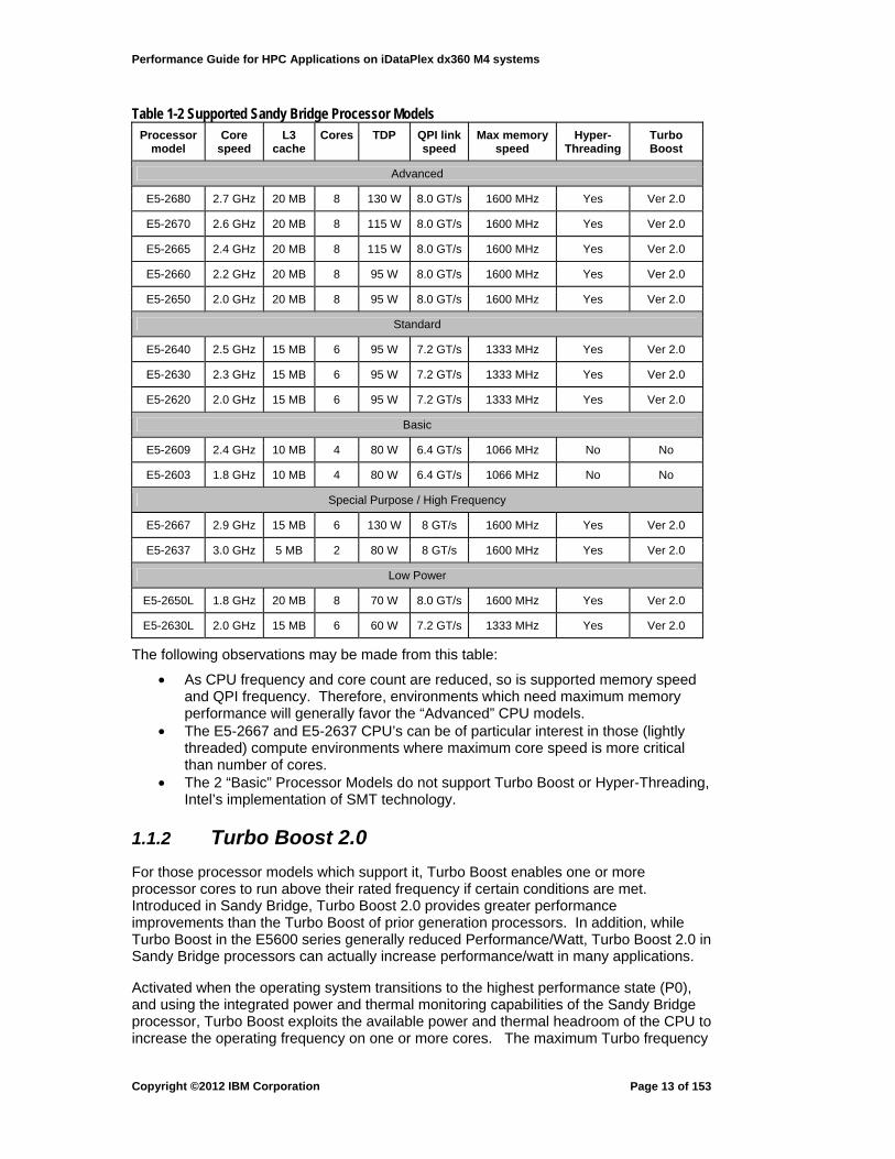
Table 1-2 Supported Sandy Bridge Processor Models Processor
model Core
speed L3
cache Cores TDP QPI link
speed Max memory
speed Hyper-
Threading Turbo Boost
Advanced
E5-2680 2.7 GHz 20 MB 8 130 W 8.0 GT/s 1600 MHz Yes Ver 2.0
E5-2670 2.6 GHz 20 MB 8 115 W 8.0 GT/s 1600 MHz Yes Ver 2.0
E5-2665 2.4 GHz 20 MB 8 115 W 8.0 GT/s 1600 MHz Yes Ver 2.0
E5-2660 2.2 GHz 20 MB 8 95 W 8.0 GT/s 1600 MHz Yes Ver 2.0
E5-2650 2.0 GHz 20 MB 8 95 W 8.0 GT/s 1600 MHz Yes Ver 2.0
Standard
E5-2640 2.5 GHz 15 MB 6 95 W 7.2 GT/s 1333 MHz Yes Ver 2.0
E5-2630 2.3 GHz 15 MB 6 95 W 7.2 GT/s 1333 MHz Yes Ver 2.0
E5-2620 2.0 GHz 15 MB 6 95 W 7.2 GT/s 1333 MHz Yes Ver 2.0
Basic
E5-2609 2.4 GHz 10 MB 4 80 W 6.4 GT/s 1066 MHz No No
E5-2603 1.8 GHz 10 MB 4 80 W 6.4 GT/s 1066 MHz No No
Special Purpose / High Frequency
E5-2667 2.9 GHz 15 MB 6 130 W 8 GT/s 1600 MHz Yes Ver 2.0
E5-2637 3.0 GHz 5 MB 2 80 W 8 GT/s 1600 MHz Yes Ver 2.0
Low Power
E5-2650L 1.8 GHz 20 MB 8 70 W 8.0 GT/s 1600 MHz Yes Ver 2.0
E5-2630L 2.0 GHz 15 MB 6 60 W 7.2 GT/s 1333 MHz Yes Ver 2.0
The following observations may be made from this table:
• As CPU frequency and core count are reduced, so is supported memory speed and QPI frequency. Therefore, environments which need maximum memory performance will generally favor the “Advanced” CPU models.
• The E5-2667 and E5-2637 CPU’s can be of particular interest in those (lightly threaded) compute environments where maximum core speed is more critical than number of cores.
• The 2 “Basic” Processor Models do not support Turbo Boost or Hyper-Threading, Intel’s implementation of SMT technology.
1.1.2 Turbo Boost 2.0
For those processor models which support it, Turbo Boost enables one or more processor cores to run above their rated frequency if certain conditions are met. Introduced in Sandy Bridge, Turbo Boost 2.0 provides greater performance improvements than the Turbo Boost of prior generation processors. In addition, while Turbo Boost in the E5600 series generally reduced Performance/Watt, Turbo Boost 2.0 in Sandy Bridge processors can actually increase performance/watt in many applications.
Activated when the operating system transitions to the highest performance state (P0), and using the integrated power and thermal monitoring capabilities of the Sandy Bridge processor, Turbo Boost exploits the available power and thermal headroom of the CPU to increase the operating frequency on one or more cores. The maximum Turbo frequency
Copyright ©2012 IBM Corporation
Page 13 of 153
Performance Guide for HPC Applications on iDataPlex dx360 M4 systems
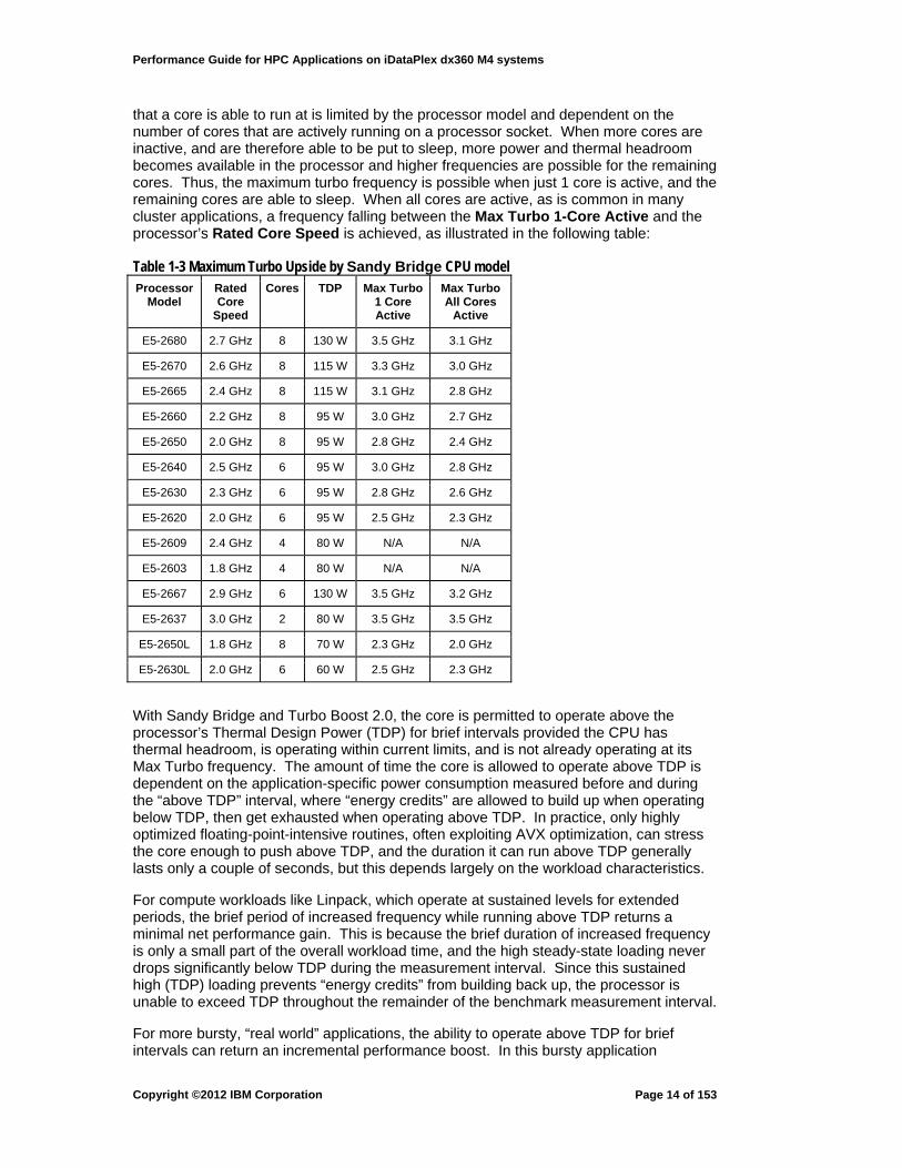
that a core is able to run at is limited by the processor model and dependent on the number of cores that are actively running on a processor socket. When more cores are inactive, and are therefore able to be put to sleep, more power and thermal headroom becomes available in the processor and higher frequencies are possible for the remaining cores. Thus, the maximum turbo frequency is possible when just 1 core is active, and the remaining cores are able to sleep. When all cores are active, as is common in many cluster applications, a frequency falling between the Max Turbo 1-Core Active and the processor’s Rated Core Speed is achieved, as illustrated in the following table:
Table 1-3 Maximum Turbo Upside by Sandy Bridge CPU model Processor
Model Rated Core
Speed
Cores TDP Max Turbo 1 Core Active
Max Turbo All Cores
Active
E5-2680 2.7 GHz 8 130 W 3.5 GHz 3.1 GHz
E5-2670 2.6 GHz 8 115 W 3.3 GHz 3.0 GHz
E5-2665 2.4 GHz 8 115 W 3.1 GHz 2.8 GHz
E5-2660 2.2 GHz 8 95 W 3.0 GHz 2.7 GHz
E5-2650 2.0 GHz 8 95 W 2.8 GHz 2.4 GHz
E5-2640 2.5 GHz 6 95 W 3.0 GHz 2.8 GHz
E5-2630 2.3 GHz 6 95 W 2.8 GHz 2.6 GHz
E5-2620 2.0 GHz 6 95 W 2.5 GHz 2.3 GHz
E5-2609 2.4 GHz 4 80 W N/A N/A
E5-2603 1.8 GHz 4 80 W N/A N/A
E5-2667 2.9 GHz 6 130 W 3.5 GHz 3.2 GHz
E5-2637 3.0 GHz 2 80 W 3.5 GHz 3.5 GHz
E5-2650L 1.8 GHz 8 70 W 2.3 GHz 2.0 GHz
E5-2630L 2.0 GHz 6 60 W 2.5 GHz 2.3 GHz
With Sandy Bridge and Turbo Boost 2.0, the core is permitted to operate above the processor’s Thermal Design Power (TDP) for brief intervals provided the CPU has thermal headroom, is operating within current limits, and is not already operating at its Max Turbo frequency. The amount of time the core is allowed to operate above TDP is dependent on the application-specific power consumption measured before and during the “above TDP” interval, where “energy credits” are allowed to build up when operating below TDP, then get exhausted when operating above TDP. In practice, only highly optimized floating-point-intensive routines, often exploiting AVX optimization, can stress the core enough to push above TDP, and the duration it can run above TDP generally lasts only a couple of seconds, but this depends largely on the workload characteristics.
For compute workloads like Linpack, which operate at sustained levels for extended periods, the brief period of increased frequency while running above TDP returns a minimal net performance gain. This is because the brief duration of increased frequency is only a small part of the overall workload time, and the high steady-state loading never drops significantly below TDP during the measurement interval. Since this sustained high (TDP) loading prevents “energy credits” from building back up, the processor is unable to exceed TDP throughout the remainder of the benchmark measurement interval.
For more bursty, “real world” applications, the ability to operate above TDP for brief intervals can return an incremental performance boost. In this bursty application
Copyright ©2012 IBM Corporation
Page 14 of 153

Performance Guide for HPC Applications on iDataPlex dx360 M4 systems
scenario, the processor spends short intervals below TDP where energy credits are able to build up, then exhausts those energy credits when operating above TDP. Because more time is spent above TDP for this case, the performance gains realized for Turbo Boost are greater.
It is important to note that the maximum Turbo Boost upsides listed in Table 1-3 are not guaranteed for all workloads. For workloads with “heavy” power and thermal characteristics, specifically AVX-optimized routines like Linpack, a processor may run at a frequency lower than its listed Max Turbo frequency. In these specific high-load workload cases, the core will run as fast as it can while staying at or under its TDP. The only frequency “guaranteed” for all workloads is the processor’s rated frequency, though in practice some portion of the Turbo Boost capability is still possible even with highly optimized AVX codes.
Finally, since any level of Turbo Boost above the “All Cores Active” frequency is dependent on at least some of the cores being in ACPI C2 or C3 sleep states, these C-States must remain enabled in system setup.
Copyright ©2012 IBM Corporation
Page 15 of 153

Performance Guide for HPC Applications on iDataPlex dx360 M4 systems
1.2 System
The dx360 M4 introduces some key system-level features enabling maximum performance levels to be sustained. By subsystem, these include:
Memory:
• 4x 1600 MHz capable DDR3 Memory Channels per processor • 2 DIMMs per memory channel • 16 total DIMMs supporting a total capacity of up to 256 GB
Processor Interconnect
• Dual QPI Interconnects, operating at up to 8 GT/s
Expansion Cards
• Each processor supplies 24 lanes of Gen3 PCIe to a PCIe riser card • Each PCIe Gen3 riser provides one x16 slot (1U riser), or one x16 slot and one
x8 slot (2U riser)
Communications
• Integrated dual port Intel 1 gigabit Ethernet controller for basic connectivity needs • Mezzanine Card options of either 10Gbit Ethernet or FDR InfiniBand, without
consuming a PCIe slot
The physical topology of these parts is depicted in the following block diagram. Note that the interconnecting buses are also shown, since understanding which CPU these buses connect to can be the key to tuning the locality of system resources.
Figure 1-2 dx360 M4 Block Diagram with Data Buses
Front of System
Not explicitly shown in this diagram, but key to many workloads, is the storage
Dual QPI Interconnects
1U Riser: +1x FHHL x16 2U Riser: +1x FHHL x8 +1x FHFL x16
4 DDR3 Memory Channels
1U Riser: +1x FHHL x16 2U Riser: +1x FHHL x8 +1x FHFL x16
4 DDR3 Memory Channels
10Gb or Infiniband
Mezz Card
PCIe Gen3 x24 To Riser Slot
PCIe Gen3 x24 To Riser Slot
SDB CPU
1
SDB CPU
0
15 16 12
3456
789 10
11 12 13 14
PCH
1Gb
Copyright ©2012 IBM Corporation
Page 16 of 153

Performance Guide for HPC Applications on iDataPlex dx360 M4 systems
connectivity. Depending on requirements, each compute node can be configured with one 3.5” SATA drive, up to two 2.5” SAS/SATA disks, or up to four 1.8” SSD’s. Connection to these drives is via two 6 Gbps SATA ports provided by the Intel C600 Chipset (PCH), or via an optional RAID card. More detail on these options can be found in the dx360 M4 Product Guide.
Note also that the dx360 M4 uses dual coherent QPI links to interconnect the CPU’s. Data traffic across these links is automatically load balanced to ensure maximum performance. Combined with up to 8 GT/s speeds, this capability enables significantly higher remote node data bandwidths than prior generation platforms.
1.2.1 I/O and Locality Considerations
While Non-Uniform Memory Architecture (NUMA) is not a new characteristic for CPU and Memory resources, the integration of the I/O bridge into the Sandy Bridge processor has introduced an added complexity for those looking to extract optimal node performance. As can be seen from Figure 1-2, the integrated 1 Gigabit Ethernet ports, high speed Mezzanine card, and the PCIe slots of the Right Side riser card are “local” to only CPU0, while the balance of the PCIe slots of the Left Side riser card are connected to CPU1.
This Non-Uniform I/O architecture enables very high performance and low latency I/O accesses to a given processor’s I/O resources, but the possibility does exist for I/O access to a “remote” processor’s resources, requiring traversal of the QPI links. While this worst-case remote I/O access is still generally faster than the best-case performance of the E5600, it is important to understand that some I/O accesses can be faster than others with this architecture. With that in mind, the end user may chose to implement I/O tuning techniques to pin the system software to local I/O resources, if maximum I/O performance is required. This may be especially important for those environments implementing GPU solutions.
Additional detail covering supported I/O adapters and GPUs is available in the dx360 M4 Product Guide
1.2.2 Memory Subsystem
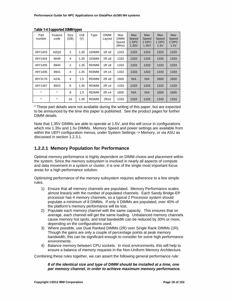
Multiple DIMM options are available to fit most application requirements, including both 1.5V 1600 MHz capable DIMMs, as well as 1.35V low power options. Unbuffered and Registered DIMMs are available to fit the reliability and performance objectives of the deployment, and capacities from 2GB to 16GB are available at product launch.
The speed that the entire memory subsystem is clocked at is determined by the lower of
1) the CPU’s maximum supported memory speed as indicated in Table 1-2 2) the speed of the slowest DIMM channel on the system.
The maximum operating speed of each DIMM channel is dependent on the capability of the DIMMs used, the speed and voltage that the DIMM is configured to run at, and the number of DIMMs on the memory channel.
A list of the dx360 M4’s supported DIMMs and the maximum frequencies that these DIMMs can operate in various configurations and power settings are listed below.
Copyright ©2012 IBM Corporation
Page 17 of 153
Performance Guide for HPC Applications on iDataPlex dx360 M4 systems
Table 1-4 Supported DIMM types Part
number Feature
code Size (GB)
Volt (V)
Type DIMM Layout
Max DIMM Speed (MHz)
Max Speed 1 DPC 1.35V
Max Speed 2 DPC 1.35V
Max Speed 1 DPC 1.5V
Max Speed 2 DPC 1.5V
49Y1403 A0QS 2 1.35 UDIMM 1R x8 1333 1333 1333 1333 1333
49Y1404 8648 4 1.35 UDIMM 2R x8 1333 1333 1333 1333 1333
49Y1405 8940 2 1.35 RDIMM 1R x8 1333 1333 1333 1333 1333
49Y1406 8941 4 1.35 RDIMM 1R x4 1333 1333 1333 1333 1333
90Y3178 A24L 4 1.5 RDIMM 2R x8 1600 N/A N/A 1600 1600
49Y1397 8923 8 1.35 RDIMM 2R x4 1333 1333 1333 1333 1333
* * 8 1.5 RDIMM 2R x4 1600 N/A N/A 1600 1600
* * 16 1.35 RDIMM 2Rx4 1333 1333 1333 1333 1333
* These part details were not available during the writing of this paper, but are expected to be announced by the time this paper is published. See the product pages for further DIMM details.
Note that 1.35V DIMMs are able to operate at 1.5V, and this will occur in configurations which mix 1.35v and 1.5v DIMMs. Memory Speed and power settings are available from within the UEFI configuration menus, under System Settings -> Memory, or via ASU as discussed in section 1.2.3.1.
1.2.2.1 Memory Population for Performance
Optimal memory performance is highly dependent on DIMM choice and placement within the system. Since the memory subsystem is involved in nearly all aspects of compute and data movement in a system or cluster, it is one of the single most important focus areas for a high performance solution.
Optimizing performance of the memory subsystem requires adherence to a few simple rules.
1) Ensure that all memory channels are populated. Memory Performance scales almost linearly with the number of populated channels. Each Sandy Bridge-EP processor has 4 memory channels, so a typical 2 Processor system should populate a minimum of 8 DIMMs. If only 4 DIMMs are populated, over 40% of the platform’s memory performance will be lost.
2) Populate each memory channel with the same capacity. This ensures that on average, each channel will get the same loading. Unbalanced memory channels cause memory hot spots, and total bandwidth can be reduced by 30% or more, depending on the configurations used.
3) Where possible, use Dual Ranked DIMMs (2R) over Single Rank DIMMs (1R). Though the gains are only a couple of percentage points at peak memory bandwidth, this can be significant enough to consider for some high performance environments.
4) Balance memory between CPU sockets. In most environments, this will help to ensure a balance of memory requests in the Non-Uniform Memory Architecture.
Combining these rules together, we can assert the following general performance rule:
8 of the identical size and type of DIMM should be installed at a time, one per memory channel, in order to achieve maximum memory performance.
Copyright ©2012 IBM Corporation
Page 18 of 153
Performance Guide for HPC Applications on iDataPlex dx360 M4 systems
Using the DIMM slot numbering as indicated in Figure 1-1 above, identical DIMMs should be installed within each of the following 8-DIMM groups:
1) DIMMs 1, 3, 6, 8 (CPU0), and DIMMs 9, 11, 14, 16 (CPU1) 2) DIMMs 2, 4, 5, 7 (CPU0), and DIMMs 10, 12, 13, 15 (CPU1)
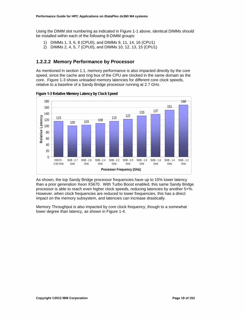
1.2.2.2 Memory Performance by Processor
As mentioned in section 1.1, memory performance is also impacted directly by the core speed, since the cache and ring bus of the CPU are clocked in the same domain as the core. Figure 1-3 shows unloaded memory latencies for different core clock speeds, relative to a baseline of a Sandy Bridge processor running at 2.7 GHz.
Figure 1-3 Relative Memory Latency by Clock Speed
115100 103 108
115 122133 137
151
168
0
20
40
60
80
100
120
140
160
180
X5670 -2.93 GHz
SDB - 2.7GHz
SDB - 2.6GHz
SDB - 2.4GHz
SDB - 2.2GHz
SDB - 2.0GHz
SDB - 1.8GHz
SDB - 1.6GHz
SDB - 1.4GHz
SDB - 1.2GHz
Processor Frequency (GHz)
Rel
ativ
e L
aten
cy
As shown, the top Sandy Bridge processor frequencies have up to 15% lower latency than a prior generation Xeon X5670. With Turbo Boost enabled, this same Sandy Bridge processor is able to reach even higher clock speeds, reducing latencies by another 5+%. However, when clock frequencies are reduced to lower frequencies, this has a direct impact on the memory subsystem, and latencies can increase drastically.
Memory Throughput is also impacted by core clock frequency, though to a somewhat lower degree than latency, as shown in Figure 1-4.
Copyright ©2012 IBM Corporation
Page 19 of 153

Performance Guide for HPC Applications on iDataPlex dx360 M4 systems
Figure 1-4 Relative Memory Throughput by Clock Speed
0
20
40
60
80
100
120
2.7 2.6 2.4 2.2 2 1.8 1.6 1.4 1.2
SDB Processor Frequency (GHz)
Rel
ativ
e M
emo
ry T
hro
ug
hp
ut
While processor ratings less than 1.8 GHz are not supported on the dx360 M4, the lower frequencies shown are possible when processor P-states are enabled, which enables a power-saving, down-clocking of the processor. While the active usage of a low frequency P-state by the OS will general occur only during periods which lack performance sensitivity, there are specific cases where this can become an issue in real workloads.
Consider the case where an application may only exercise one processor socket (NUMA node) at a time. In this case, the 2nd processor socket may be allowed to downclock, or even sleep, assuming these capabilities are enabled in the System Settings and the OS. However, cache coherency operations and remote memory requests may still take place to the 2nd processor, which now has a critical component of its cache and memory subsystem, the ring bus, being clocked at a reduced speed. For this reason, environments which may have this sort of unbalanced processor loading occurring, specifically while demanding peak memory performance, may consider disabling processor P-states within System Settings, or setting the minimum processor frequency within the OS. This latter method is explained for Linux OS here.
1.2.3 UEFI
The platform UEFI, working in conjunction with the Integrated Management Module, is responsible for control of the low level “hardware” system settings. Many of the tunings used to optimize performance are available within the F1 – System Setup menu, presented during boot time. These settings are also available from a command line interface using the IBM Advanced Settings Utility, or ASU.
Since the dx360 M4 is used in cluster deployments, this section will first introduce the ASU tool scripting tool, then provide UEFI tunings as implemented in ASU.
1.2.3.1 ASU
The Advanced Settings Utility is a key platform tuning and management mechanism to read and write system configuration settings without having to manually enter “F1 Setup” menus at boot time. Though changes to ASU settings still generally require a system reboot to apply, this utility allows a consistent tuning of platforms and clusters using either manual command line execution, or automated scripting.
Copyright ©2012 IBM Corporation
Page 20 of 153

Performance Guide for HPC Applications on iDataPlex dx360 M4 systems
Basic ASU commands To capture all ASU supported system settings: asu show all To show permitted values of a specific setting: asu showvalues <setting> To set a setting to one of the permitted values: asu set <setting> <value> To apply a batch of settings from a file: asu batch <file name>
batch file format per line: set <setting> <value>
If <value> contains spaces, be sure to enclose the value string in parentheses, ex:
asu set OperatingModes.ChooseOperatingMode “Maximum Performance”
All the above commands can be issued from a remote host, by appending the following:
--host <IMM IP Address> --user <IMM userid> --password <IMM password>
Note that for 64-bit OS’s, the asu binary name is asu64
Further information on ASU, including links to download Linux and Windows versions of the tool are located here.
The ASU Users Guide can be found here.
1.2.3.2 UEFI Tunings
While the F1 System Setup menu and “asu show all” commands provide numerous configuration parameters, there are few key parameters that are of particular interest for high performance computing.
Many environments will not need explicit control over individual platform settings with Sandy Bridge, as the dx360 M4 can be optimized for most environments with just a couple of simple settings. For most environments, the UEFI enables four “Operating Modes” which will cover the tuning requirements for many of the common usage scenarios. These are:
1) Minimal Power This mode reduces memory and QPI speeds, and activates the most aggressive power management features, the combination of which will have steep performance implications. This setting would be recommended for those environments which must minimize power consumption at all costs.
2) Efficiency – Favor Power This mode also limits QPI and memory speeds, but not as aggressively as Minimal Power mode. Turbo Mode remains disabled in this operating mode.
3) Efficiency – Favor Performance (System Default) This is the default operating mode. Memory and QPI buses are run at their maximum hardware supported speeds, though most power management features remain enabled. Turbo mode is enabled, and processor sleep states (C-States) are enabled and allowed to enter the deepest sleep levels. This mode generally enables an optimal balance of performance/watt on Sandy Bridge.
4) Maximum Performance This mode generally allows the highest performance levels for most applications, though exceptions do occur. Processor C-States continue to remain enabled, as these are necessary for optimal Turbo Mode performance. The C-State Limit is reduced to ACPI C2 in this mode to minimize the latency associated with waking the sleeping cores, and C1 Enhanced Mode is disabled. Processor Performance
Copyright ©2012 IBM Corporation
Page 21 of 153

Performance Guide for HPC Applications on iDataPlex dx360 M4 systems
States are disabled in this mode, ensuring the CPU is always operating at or above rated frequency.
There is also a 5th, “Custom Mode”, which enables all of the UEFI features to be set individually for specific workload conditions. The following table covers the most common performance-specific parameters, listed in ASU setting format:
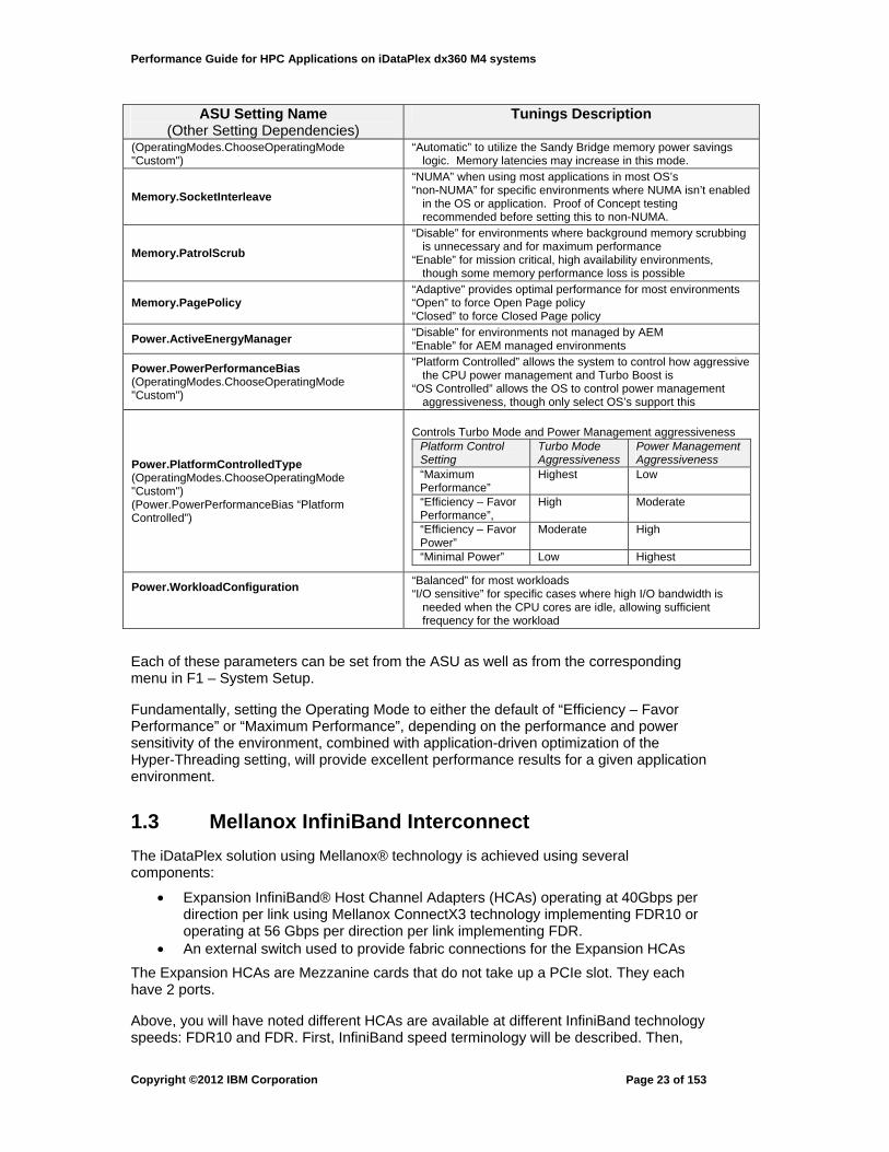
Table 1-5 Common UEFI Performance Tunings ASU Setting Name
(Other Setting Dependencies) Tunings Description
OperatingModes.ChooseOperatingMode
“Custom” is required for most of the parameters below to be enabled (i.e. those indicating this mode as a dependency)
“Maximum Performance” sets Operating Mode as per above “Efficiency – Favor Performance” sets Operating Mode as per
above “Efficiency – Favor Power” sets Operating Mode as per above “Minimal Power” sets Operating Mode as per above
Processors.Hyper-Threading “Enable” for general purpose applications “Disable” for some highly core-efficient HPC workloads
Processors.HardwarePrefetcher “Enable” for most environments “Disable” used rarely, only with aggressive software prefetching
Processors.AdjacentCachePrefetch “Enable” for most environments “Disable” used rarely, only with aggressive software prefetching
Processors.DCUStreamerPrefetcher “Enable” for most environments “Disable” used rarely, only with aggressive software prefetching
Processors.DCUIPPrefetcher “Enable” for most environments “Disable” used rarely, only with aggressive software prefetching
Processors.TurboMode (OperatingModes.ChooseOperatingMode "Custom")
“Enable” for performance and performance/watt centric environments
“Disable” where minimum power consumption is required
Processors.ProcessorPerformanceStates (OperatingModes.ChooseOperatingMode "Custom")
“Disable” prevents processor down-clocking, improving performance in some environments at the expense of increased power consumption
“Enable” allows processor to down-clock, saving power
Processors.C-States (OperatingModes.ChooseOperatingMode "Custom")
“Enable” allows processor to enter deep sleep states, saving power and allowing maximum Turbo Mode frequency
“Disable” prevents deep sleep states and any potential “wake up” latency, but will also prevent Turbo Boost from going over the “All Cores Active” frequency.
Processors.PackageACPIC-StateLimit (Processors.C-States Enable) (OperatingModes.ChooseOperatingMode "Custom")
“ACPI C2” is the first “deep” sleep state, mapped to Intel’s C3 state, the core PLLs are turned off and caches are flushed.
“ACPI C3” is the deepest sleep state, mapped to Intel’s C6 state, saves the core state to LLC and uses power gating to significantly reduce core power consumption. This state has a higher “wake up” latency than ACPI C2.
Processors.C1EnhancedMode (OperatingModes.ChooseOperatingMode "Custom")
“Disable” to eliminate the possibility of “wake up” latencies affecting an application environment, at the cost of additional power usage
“Enable” allows the cores to enter the halt state. Even in this state, Turbo Boost considers this an active core, though some power savings are realized. Some compute environments may see small performance impacts from enabling this setting
Processors.QPILinkFrequency (OperatingModes.ChooseOperatingMode "Custom")
"Max Performance" sets QPI to the maximum supported frequency
“Balanced” reduces QPI frequency by one stepping “Minimal Power” reduces QPI frequency to the lowest supported speed
Memory.MemorySpeed (OperatingModes.ChooseOperatingMode "Custom")
“Max Performance” sets memory to the fastest hardware supported speed
“Balanced” reduces memory speed for some DIMMs, but enables some power savings
“Minimal Power” runs memory in the lowest power mode, at the expense of performance
Memory.MemoryPowerManagement “Disable” for best performance
Copyright ©2012 IBM Corporation
Page 22 of 153
Performance Guide for HPC Applications on iDataPlex dx360 M4 systems
ASU Setting Name Tunings Description (Other Setting Dependencies)
(OperatingModes.ChooseOperatingMode "Custom")
“Automatic” to utilize the Sandy Bridge memory power savings logic. Memory latencies may increase in this mode.
Memory.SocketInterleave
“NUMA” when using most applications in most OS’s “non-NUMA” for specific environments where NUMA isn’t enabled
in the OS or application. Proof of Concept testing recommended before setting this to non-NUMA.
Memory.PatrolScrub
“Disable” for environments where background memory scrubbing is unnecessary and for maximum performance
“Enable” for mission critical, high availability environments, though some memory performance loss is possible
Memory.PagePolicy “Adaptive” provides optimal performance for most environments “Open” to force Open Page policy “Closed” to force Closed Page policy
Power.ActiveEnergyManager “Disable” for environments not managed by AEM “Enable” for AEM managed environments
Power.PowerPerformanceBias (OperatingModes.ChooseOperatingMode "Custom")
“Platform Controlled” allows the system to control how aggressive the CPU power management and Turbo Boost is
“OS Controlled” allows the OS to control power management aggressiveness, though only select OS’s support this
Power.PlatformControlledType (OperatingModes.ChooseOperatingMode "Custom") (Power.PowerPerformanceBias “Platform Controlled”)
Controls Turbo Mode and Power Management aggressiveness Platform Control Setting
Turbo Mode Aggressiveness
Power Management Aggressiveness
“Maximum Performance”
Highest Low
“Efficiency – Favor Performance”,
High Moderate
“Efficiency – Favor Power”
Moderate High
“Minimal Power” Low Highest
Power.WorkloadConfiguration
“Balanced” for most workloads “I/O sensitive” for specific cases where high I/O bandwidth is
needed when the CPU cores are idle, allowing sufficient frequency for the workload
Each of these parameters can be set from the ASU as well as from the corresponding menu in F1 – System Setup.
Fundamentally, setting the Operating Mode to either the default of “Efficiency – Favor Performance” or “Maximum Performance”, depending on the performance and power sensitivity of the environment, combined with application-driven optimization of the Hyper-Threading setting, will provide excellent performance results for a given application environment.
1.3 Mellanox InfiniBand Interconnect
The iDataPlex solution using Mellanox® technology is achieved using several components:
• Expansion InfiniBand® Host Channel Adapters (HCAs) operating at 40Gbps per direction per link using Mellanox ConnectX3 technology implementing FDR10 or operating at 56 Gbps per direction per link implementing FDR.
• An external switch used to provide fabric connections for the Expansion HCAs
The Expansion HCAs are Mezzanine cards that do not take up a PCIe slot. They each have 2 ports.
Above, you will have noted different HCAs are available at different InfiniBand technology speeds: FDR10 and FDR. First, InfiniBand speed terminology will be described. Then,
Copyright ©2012 IBM Corporation
Page 23 of 153

Performance Guide for HPC Applications on iDataPlex dx360 M4 systems
FDR10 will be described. Then, FDR will be described.
The base data rate for InfiniBand technology has been the single data rate (SDR), which is 2.5Gbps per lane or bit in a link. Previous interconnect technologies, up to FDR10, have used this SDR reference speed. The standard width of the interface is 4X or 4 bits wide. Therefore, the standard SDR bandwidth or speed of a link is 2.5Gbps times 4 bit lanes, or 10Gbps. DDR, or double data rate, is 20Gbps per 4x link. QDR, or quad data rate, is 40Gbps per link.
FDR10 is based off of FDR technology with the “10” appended to FDR to directly indicate the bit lane speed of 10Gbps. An important difference between FDR10 and QDR is that FDR10 is more efficient in its data transfer than QDR, because of certain FDR characteristics.
The FDR nomenclature begins to deviate from basing the speed on a multiple of 2.5Gbps. FDR stands for fourteen data rate, or a bit speed of 14Gbps, which translates into a 4x link speed of 56Gbps.
More information on InfiniBand architecture is available on the InfiniBand Trade Association® (IBTA) website at http://infinibandta.org
While FDR10 is nominally the same speed (40Gbps per 4x link) as the previous generation (QDR), there is a different encoding of the data on the link that allows for more efficient use of the link while still providing data protection. The QDR technology ran an 8/10 bit encoding which yields 80% efficiency for every bit of data payload sent across the link. FDR10 uses a 64/66 bit encoding which yields 97% efficiency. In other words, the effective rate of a QDR link is 32Gbps; whereas, FDR10 has an effective data rate of 38.8 Gbps. In both cases, the effective data rate is also used by a modest number of bits implementing packet overhead.
By using the same nominal speed as QDR, FDR10 can use the same basic cable technology as QDR, which has helped with getting the improved FDR link efficiency to market quicker.
To achieve FDR10 efficiencies, the HCAs must be attached to switches that support FDR bit encoding. If they are attached to QDR switches, the HCAs will operate, but at QDR rates and efficiencies.
FDR operates at 56Gbps per 4x link. It maintains the same bit encoding as FDR10 and therefore the same 97% efficiency of the link. This yields an effective data rate of 54.3 Gbps. To achieve full FDR rates, the HCAs must be attached to switches that support full FDR rates. If they are attached to switches that support a maximum of QDR or FDR10 rates, the HCAs will operate, but at the lower speeds.
The Mellanox model numbers for currently supported FDR10/FDR switches are:
• SX6036 = a 36 port Edge switch.
• SX6536 = a 648 port Director switch, which scales from 8.64 Tbps up to 72.52 Tbps of bandwidth in a single enclosure.
Both switch models are non-blocking. Both switch models can support any speed up to FDR (including FDR10).
Edge switches are typically used for small clusters of servers or as top-of-rack switches that provide edge or leaf connectivity to one or more Director switches implemented as core switches. This allows for scaling beyond 648 nodes.
It is also possible to use the SX6536 to connect up to 648 HCAs in a single InfiniBand
Copyright ©2012 IBM Corporation
Page 24 of 153

Performance Guide for HPC Applications on iDataPlex dx360 M4 systems
subnet, or plane.
The typical large scale solution is implemented as a fat-tree to maintain 100% bi-sectional bandwidth for any to any node communication. For example, for a cluster of 1296 nodes, each with one connection into a plane, the typical topology would be to have 72 SX6036 Edge switches distributed amongst the frames of DX360 M4 servers. This has 18 servers connected to each Edge switch. The Edge switches will then connect to two SX6536 Director switches with 9 cables from each of the Edge switches connecting to each of the Director switches.
It is possible to over-subscribe switch connectivity to reduce the number of required switches in very large fabrics, and thus reduce cost. However, care must be taken in doing this for solutions that require any node to communicate with any other node in a random fashion, because the oversubscribed networks can cause data traffic congestion. However, if data patterns are well understood from the onset, or if applications run on only portions of the cluster, then it may be possible to design an oversubscribed fabric that does not lead to excessive congestion.
Another consideration in implementing the InfiniBand interconnect is configuring the subnet manager. Some considerations are alternative routing algorithms, alternative MTU settings, and Quality of Service functions.
Various subnet managers typically have several possible routing algorithms such as Minimum number of Hops (default), up-down, fat tree, and so on. It is recommended that the various options be discussed with a routing expert before deviating from the default algorithm. Parameters like the types of applications, the chosen topology and the experiences of a particular algorithm in the field should be considered.
Some current options for Mellanox routing methods are:
MINHOP or shortest path optimizes routing to achieve the shortest path between two nodes. It balances routing based on the number of paths using each port in the fabric. This is the default algorithm.
UPDN or up-down provides a shortest path optimization, but also considers a set of ranking rules. This is designed for a topology that is not a pure Fat tree, and has potential deadlock loops that must be avoided.
FAT TREE can be used for various fat-tree topologies as it optimizes for various congestion-free communication patterns. It is similar to UPDN in that it also employs ranking rules.
LASH or layered shortest path uses InfiniBand virtual layers (SL) to provide dead-lock free shortest path routing.
DOR or dimension ordered routing provides deadlock free routes for hypercube and mesh topologies.
FILE or file-based loads the routing information directly from a file. This would be for very specialized applications and has disadvantages in that it restricts the subnet manager’s ability to dynamically react to changes in the topology.
UFM TARA or traffic aware routing is unique to Mellanox’s Unified Fabric Manager® (UFM) and combines UPDN with traffic-aware balancing that includes application topology and weighted patterns. This requires UFM to work in concert with applications and job managers to maintain awareness of traffic patterns so that it can dynamically optimize routing. Therefore, it may not be possible to use this algorithm with all solutions.
Copyright ©2012 IBM Corporation
Page 25 of 153

Performance Guide for HPC Applications on iDataPlex dx360 M4 systems
The Mellanox subnet manager also includes support for adaptive routing. Adaptive routing allows the switch to choose how to route a packet based on availability of the optional ports used to get from one node to another. This works as you traverse the fabric from the source node to halfway out in the fabric. Once you reach the halfway point, the remainder of the path is predestined and no more choices are available. If the congestion pattern tends to be in the first half of the route, this can be an effective tool. If the congestion pattern is in the back half of the route, adaptive routing is less effective – for example, for many-to-one patterns, the congestion starts at the destination node end and backs up into the fabric.
The Mellanox subnet manager also includes support for Quality of Service (QoS). It uses service lanes (or virtual lanes) and a weight factor for each lane to ensure that higher priority data traffic is separated from and takes precedence over lower priority data traffic. In this way, the higher priority traffic avoids being delayed by lower priority traffic. To take advantage of QoS, the applications, MPI and RDMA stack must be implemented in a way that uses service lanes. As this is not always the case, some solutions are limited to separating IP over InfiniBand (IPoIB) traffic from RDMA traffic by taking advantage of the ability to assign a non-default service lane for IPoIB.
For certain applications it may be possible to improve performance by using a non-default InfiniBand link MTU or multicast MTU. The default is 2K, but some success has been seen in the past with 4K. Typically, the starting MTU should be 2K and only adjusted to 4K if performance targets are not being achieved. Also, a performance expert should be consulted about the MPI solution before attempting a non-default MTU setting.
Note: The InfiniBand MTU is different from an IP MTU. It is a maximum transmission unit at the physical layer, or the size of packets in the fabric itself. Larger IP packets bound by the IP MTU are broken down into smaller packets in the physical layer bound by the InfiniBand MTU.
While it is not often used in the industry, smaller fabric solutions can sometimes benefit from LMC (LID mask control) being set to 1 or 2. A non-zero LMC causes the SM to assign multiple LIDs to each device, and then generate a different path to each LID. While originally envisioned as a failover mechanism, this also allows for upper layer protocols to scatter traffic over several paths with the intention of reducing congestion. This requires an RDMA stack that is aware of the multiple paths provided by a non-zero LMC so that the path can be periodically switched according to some algorithm (like round-robin, or least recently used). There is a cost associated with LMC > 0, in that each port is assigned multiple LIDs (local identifiers) and this will take up more buffer and memory space. It will also affect start-up time for RC (reliable) connections. As a cluster is scaled up, the impact becomes more noticeable. In fact, if a cluster gets large enough, the hardware may run out of space to support the number of buffers required for LMC > 0. Typically, a performance expert should be consulted on the MPI solution to see if there is any benefit to LMC > 0.
Finally, a pro-active method for monitoring the health of the fabric can help maintain performance. With the current InfiniBand architecture, errors in the fabric require a retransmission from source to destination. This can be costly in terms of latency and lost effective bandwidth as packets are retransmitted. Again, the recommendation is to consult with an expert in fabric monitoring to understand how best to determine that the network fabric is healthy. Some considerations are:
• Monitoring error counters and choosing thresholds that are appropriate for the expected bit error rate (BER) of the fabric technology. Typically, default thresholds are only adequate for links that greatly exceed the acceptable BER. For links that are noisy and can impact performance, but are barely over the acceptable BER, default thresholds are likely to be inadequate. A
Copyright ©2012 IBM Corporation
Page 26 of 153

Performance Guide for HPC Applications on iDataPlex dx360 M4 systems
time based threshold is preferred. However, many basic monitoring tools only have count based thresholds (ignoring the bit error rate), which leads to the need to develop a local strategy for regularly clearing the error counters to impose a rough time-base to the count threshold. An expert should be consulted for the appropriate bit error rate. In many cases, this is currently in the 10-15 to 10-14 range.
• Monitoring for lost links in the fabric that can lead to imbalanced routes and congestion.
• Monitoring link speeds and widths. When a link is established it is trained to the highest speed at which it can operate based on both the inherent limitations of the technology (FDR10, FDR, QDR, and so on) as well as the particular instance of hardware on the link. A noisy cable or port may be tuned to a lower speed or smaller width to allow it to operate. Quite often the switch technology will allow a system administrator to override this and force a link to operate only at the maximum. However, the default case is to tune to whatever the link can handle. Therefore, unless the default is overridden, the system administrator will want to be sure to monitor for speed or width changes (particular across node or switch reboots).For FDR10, it is particularly important to be observant regarding whether or not the link has come up at FDR10 versus QDR. It is possible that the link can handle 10Gbps per bit lane, but not tune to the 64/66 bit encoding. Various tools will vary in reporting whether 10Gbps is QDR or FDR10 – some will only report if it is sub-optimal.
1.3.1 References
[1] InfiniBand Linux SW Stack
[2] Routing Algorithm Info (Requires a userid with Mellanox support access).
Copyright ©2012 IBM Corporation
Page 27 of 153

Performance Guide for HPC Applications on iDataPlex dx360 M4 systems
2 Performance Optimization on the CPU
Compilers are the basic tools applied to HPC applications to get good performance from the target hardware. Usually, several compilers are available for each architecture. The first section of this chapter discusses uses of the widely adopted open source GNU compiler suite and the proprietary Intel compiler suite. Other alternatives are listed but not described.
Along with compilers, mathematical libraries are heavily used in HPC codes and are critical for high performance. Section 2.2 introduces the Intel MKL library optimized for Intel processors and briefly mentions the other alternatives.
The most important languages for High Performance Computing are FORTRAN, C, and C++ because they are the ones used by the vast majority of codes. This chapter focuses on those languages, though compiler providers also support others.
All of the descriptions of the GNU and Intel compiler options included in the tables in this chapter are taken from the GNU Optimization Options Guide and the Intel Fortran Compiler User and Reference Guide.
2.1 Compilers
2.1.1 GNU compiler
The GNU compiler tool chain contains front ends for C, C++, Objective-C, FORTRAN, Java, Ada, and Go, as well as libraries for these languages. These compilers are 100% free software and can be used on any system independently of the type of hardware. It is the default compiler for the Linux operating system and is shipped with it.
The support of AVX vector units introduced with Sandy Bridge processor has been announced with the 4.6.3 release of GCC compilers. With GCC version 4.7.0 several new features have been implemented, detailed in the compiler option section below.
In the following, we are focusing on gfortran version 4.7.0.
GCC 4.7.0 has been successfully built on a Sandy Bridge system by using the following configure options:
export BASEDIR=/path/to/GCC-4.7.0 export LD_LIBRARY_PATH=${BASEDIR}/dlibs/lib:$LD_LIBRARY_PATH ${BASEDIR}/gcc-4.7.0-RC-20120314/configure \ -–prefix=${BASEDIR}/install \ --with-gmp=${BASEDIR}/dlibs \ --with-gmp-lib=${BASEDIR}/dlibs/lib \ --with-mpfr-lib=${BASEDIR}/dlibs/lib \ --with-mpfr=${BASEDIR}/dlibs \ --with-mpc-lib=${BASEDIR}/dlibs/lib \ --with-mpc=${BASEDIR}/dlibs \ --with-ppl=${BASEDIR}/dlibs \ --with-ppl-lib=${BASEDIR}/dlibs/lib \ --with-libelf=${BASEDIR}/dlibs \ --enable-languages=c,c++,fortran --enable-shared --enable-threads=posix \ --enable-checking=release --with-system-zlib --enable-__cxa_atexit \ --disable-libunwind-exceptions --enable-libgcj-multifile
Copyright ©2012 IBM Corporation
Page 28 of 153

Performance Guide for HPC Applications on iDataPlex dx360 M4 systems
2.1.2 Intel Compiler
The Intel compiler suite is traditionally the most efficient compiler for the Intel processors as it is designed by Intel. The latest features of the Intel Sandy Bridge processor are implemented in the current version of the Intel Composer XE product version 12.1. It includes a FORTRAN, C, and C++ compiler, an MKL library and other components (Cilk, IPP, TBB, etc.)
Several additional tools are available to help analyzing and optimizing HPC codes on Intel systems. These tools are described in Chapter5.
2.1.3 Recommended compiler options
In this section the compiler options which have the greatest impact on improving the performance of HPC applications are presented. The compiler reference documents can be consulted for a full list of options,
The options can be separated into categories: architectures, general optimization, vectorization, inter procedural optimization, shared memory, and distributed parallelization. These are the most important options for improving the performance of a HPC application.
2.1.3.1 Architecture
In order to efficiently optimize a program on a specific processor, the compiler needs information on the architecture’s details. It is then able to use adapted parameters for its internal optimization engines and generate optimized assembly code matching the identified hardware as perfectly as possible: cache sizes, vector unit details, prefetching engines, etc.
If compiling on the same architecture as the one used for the computation, compilers (through usage of compiler options) can also automatically detect the processor details and then generate optimal settings without user interaction.
For cross compiling, the user has to specify the target architecture to the compiler.
Another case is when user wants to have a binary that can run on all architectures in the processor family (for instance, the x86 family). This is best applied for creating binaries for pre- or post-processing programs that don’t require significant computing power but can be conveniently run on various systems within the same processor family without recompilation.
2.1.3.1.1 GNU
The following options are used by GNU compiler to specify the hardware architecture to be used for code generation:
-march= Generate code for given CPU -mtune= Schedule code for given CPU
The “corei7-avx” argument tells the compiler to generate code for Sandy Bridge and use AVX instructions:
-march=corei7-avx
By default, it also enables the -mavx compiler flag for autovectorization.
Copyright ©2012 IBM Corporation
Page 29 of 153

Performance Guide for HPC Applications on iDataPlex dx360 M4 systems
Table 2-1 summarizes the other options that are available:
Table 2-1 GNU compiler processor-specific optimization options
-mavx Support MMX, SSE, SSE2, SSE3, SSSE3, SSE4.1, SSE4.2 and AVX built-in functions and code generation
-mavx256-split-unaligned-load Split 32-byte AVX unaligned loads
-mavx256-split-unaligned-store Split 32-byte AVX unaligned stores
-mfma Support MMX, SSE, SSE2, SSE3, SSSE3, SSE4.1, SSE4.2, AVX and FMA3 built-in functions and code generation
-mfma4 Support FMA4 built-in functions and code generation
-mprefer-avx128 Use 128-bit AVX instructions instead of 256-bit
2.1.3.1.2 Intel
For local or cross compilation, the “-xcode” option specifies the hardware architecture (“code” in this example) to be used for code generation. For the Sandy Bridge architecture, using
-xAVX
may generate SIMD instructions for Intel® processors.
If the code is being compiled on the same processor that will be used for computation (local compilation), the following option produces optimized code:
-xhost
It tells the compiler to generate instructions for the most complete instruction set available on the host processor.
For compatibility with GCC, the Intel compiler accepts GNU syntax for some options; the -mavx and -march=corei7-avx flags are equivalent to -xAVX
Options -x and -m are mutually exclusive. If both are specified, the compiler uses the last one specified and generates a warning.
The Intel compiler ignores the options in Table 2-2. These options only generate a warning message. The suggested replacement options should be used instead.
Table 2-2 A mapping between GCC and Intel compiler options for processor architectures
GCC Compatibility Option Suggested Replacement Option
-mfma -march=core-avx2
-mbmi, -mavx2, -mlzcnt -march=core-avx2
-mmovbe -march=atom -minstruction=movbe
-mcrc32, -maes, -mpclmul, -mpopcnt -march=corei7
Copyright ©2012 IBM Corporation
Page 30 of 153

Performance Guide for HPC Applications on iDataPlex dx360 M4 systems
GCC Compatibility Option Suggested Replacement Option
-mvzeroupper -march=corei7-avx
-mfsgsbase, -mrdrnd, -mf16c -march=core-avx-i
2.1.3.2 General optimization
All compilers support several levels of optimization that can be applied to source code. The more aggressive the optimization level, the faster the code runs but with a higher risk of generating significant numerical differences in the results. Balancing performance against numerical consistency is the code owner’s responsibility.
The Intel compiler includes many compiler options that can affect the optimization and the subsequent performance of the code, but this section only touches on the most common options.
2.1.3.2.1 GNU
The GCC/GFortran compiler has to be configured and compiled on a specific target system, so it may not support some features and compiler technologies depending on the configure arguments. The compiler explicitly reports on the exact set of optimizations that are enabled at each level by including the –Q –help=optimizers option:
$ gfortran -Q --help=optimizers
The general optimization levels are listed in Table 2-3
Table 2-3 General GNU compiler optimization options
GCC compiler option Explanation
-O0 Reduce compilation time and keep execution in the same order as the source line listing so that debugging produces the expected results. This is the default.
Copyright ©2012 IBM Corporation
Page 31 of 153
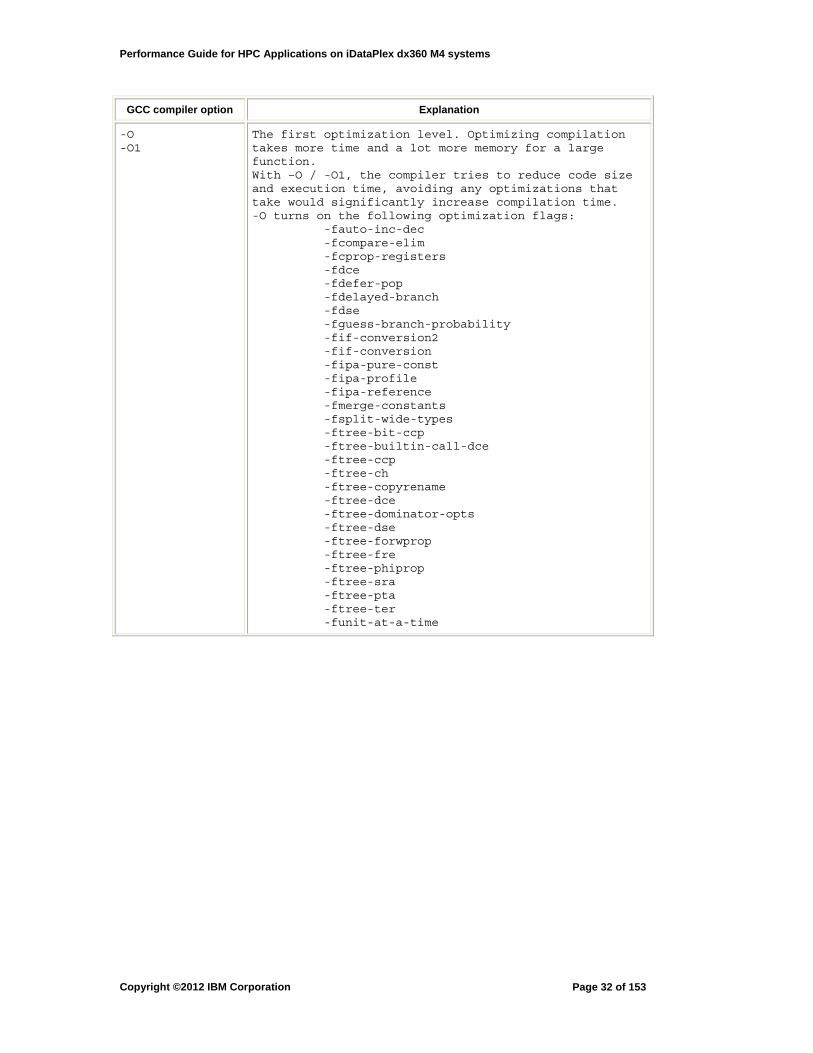
Performance Guide for HPC Applications on iDataPlex dx360 M4 systems
GCC compiler option Explanation
-O -O1
The first optimization level. Optimizing compilation takes more time and a lot more memory for a large function. With –O / -O1, the compiler tries to reduce code size and execution time, avoiding any optimizations that take would significantly increase compilation time. -O turns on the following optimization flags: -fauto-inc-dec -fcompare-elim -fcprop-registers -fdce -fdefer-pop -fdelayed-branch -fdse -fguess-branch-probability -fif-conversion2 -fif-conversion -fipa-pure-const -fipa-profile -fipa-reference -fmerge-constants -fsplit-wide-types -ftree-bit-ccp -ftree-builtin-call-dce -ftree-ccp -ftree-ch -ftree-copyrename -ftree-dce -ftree-dominator-opts -ftree-dse -ftree-forwprop -ftree-fre -ftree-phiprop -ftree-sra -ftree-pta -ftree-ter -funit-at-a-time
Copyright ©2012 IBM Corporation
Page 32 of 153
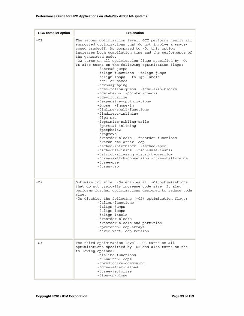
Performance Guide for HPC Applications on iDataPlex dx360 M4 systems
GCC compiler option Explanation
-O2
The second optimization level. GCC performs nearly all supported optimizations that do not involve a space-speed tradeoff. As compared to -O, this option increases both compilation time and the performance of the generated code. -O2 turns on all optimization flags specified by -O. It also turns on the following optimization flags: -fthread-jumps -falign-functions -falign-jumps -falign-loops -falign-labels -fcaller-saves -fcrossjumping -fcse-follow-jumps -fcse-skip-blocks -fdelete-null-pointer-checks -fdevirtualize -fexpensive-optimizations -fgcse -fgcse-lm -finline-small-functions -findirect-inlining -fipa-sra -foptimize-sibling-calls -fpartial-inlining -fpeephole2 -fregmove -freorder-blocks -freorder-functions -frerun-cse-after-loop -fsched-interblock -fsched-spec -fschedule-insns -fschedule-insns2 -fstrict-aliasing -fstrict-overflow -ftree-switch-conversion -ftree-tail-merge -ftree-pre -ftree-vrp
-Os
Optimize for size. -Os enables all -O2 optimizations that do not typically increase code size. It also performs further optimizations designed to reduce code size. -Os disables the following (-O2) optimization flags: -falign-functions -falign-jumps -falign-loops -falign-labels -freorder-blocks -freorder-blocks-and-partition -fprefetch-loop-arrays -ftree-vect-loop-version
-O3
The third optimization level. -O3 turns on all optimizations specified by -O2 and also turns on the following options: -finline-functions -funswitch-loops -fpredictive-commoning -fgcse-after-reload -ftree-vectorize -fipa-cp-clone
Copyright ©2012 IBM Corporation
Page 33 of 153
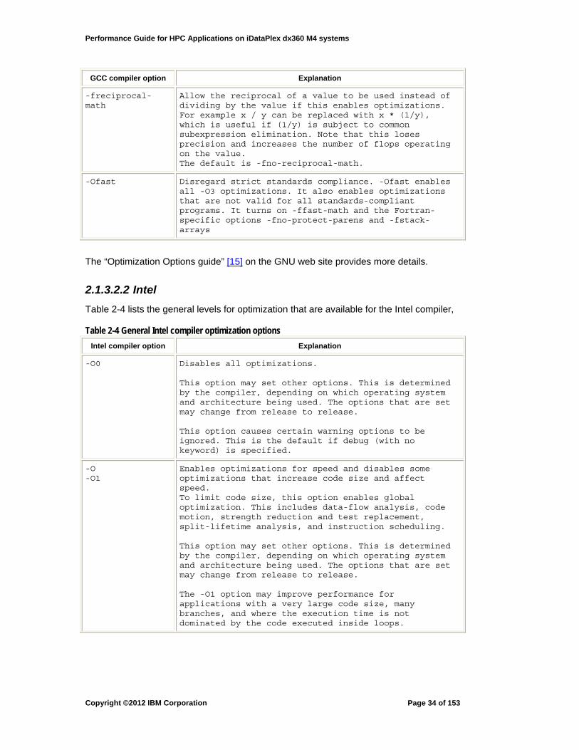
Performance Guide for HPC Applications on iDataPlex dx360 M4 systems
GCC compiler option Explanation
-freciprocal-math
Allow the reciprocal of a value to be used instead of dividing by the value if this enables optimizations. For example x / y can be replaced with x * (1/y), which is useful if (1/y) is subject to common subexpression elimination. Note that this loses precision and increases the number of flops operating on the value. The default is -fno-reciprocal-math.
-Ofast
Disregard strict standards compliance. -Ofast enables all -O3 optimizations. It also enables optimizations that are not valid for all standards-compliant programs. It turns on -ffast-math and the Fortran-specific options -fno-protect-parens and -fstack-arrays
The “Optimization Options guide” [15] on the GNU web site provides more details.
2.1.3.2.2 Intel
Table 2-4 lists the general levels for optimization that are available for the Intel compiler,
Table 2-4 General Intel compiler optimization options
Intel compiler option Explanation
-O0 Disables all optimizations. This option may set other options. This is determined by the compiler, depending on which operating system and architecture being used. The options that are set may change from release to release. This option causes certain warning options to be ignored. This is the default if debug (with no keyword) is specified.
-O -O1
Enables optimizations for speed and disables some optimizations that increase code size and affect speed. To limit code size, this option enables global optimization. This includes data-flow analysis, code motion, strength reduction and test replacement, split-lifetime analysis, and instruction scheduling. This option may set other options. This is determined by the compiler, depending on which operating system and architecture being used. The options that are set may change from release to release. The -O1 option may improve performance for applications with a very large code size, many branches, and where the execution time is not dominated by the code executed inside loops.
Copyright ©2012 IBM Corporation
Page 34 of 153

Performance Guide for HPC Applications on iDataPlex dx360 M4 systems
Intel compiler option Explanation
-O2
Enables optimizations for speed. This is the default, and generally recommended, optimization level. Vectorization is enabled at -O2 and higher levels. Some basic loop optimizations such as distribution, predicate optimization, interchange, multi-versioning, and scalar replacements are performed. This option also enables: - Inlining of intrinsic functions - Intra-file interprocedural optimization, which includes inlining, constant propagation, etc. - dead-code elimination - global register allocation - global instruction scheduling and control speculation - loop unrolling - optimized code selection - partial redundancy elimination This option may set other options, especially options that optimize for code speed. This is determined by the compiler, depending on which operating system and architecture being used. The options that are set may change from release to release. If -g is specified, -O2 is turned off and -O0 is the default unless -O2 (or -O1 or -O3) is explicitly specified in the command line together with -g. Many routines in the shared libraries are more highly optimized for Intel® microprocessors than for non-Intel microprocessors.
-Os This option enables optimizations that do not increase code size and produces a smaller code size than -O2. It disables some optimizations that increase code size for a small speed benefit. This option tells the compiler to favor transformations that reduce code size over transformations that produce maximum performance.
Copyright ©2012 IBM Corporation
Page 35 of 153
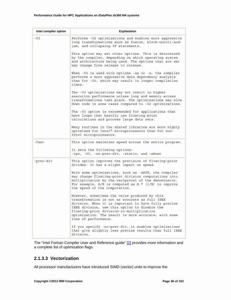
Performance Guide for HPC Applications on iDataPlex dx360 M4 systems
Intel compiler option Explanation
-O3
Performs -O2 optimizations and enables more aggressive loop transformations such as fusion, block-unroll-and-jam, and collapsing IF statements. This option may set other options. This is determined by the compiler, depending on which operating system and architecture being used. The options that are set may change from release to release. When -O3 is used with options -ax or -x, the compiler performs a more aggressive data dependency analysis than for -O2, which may result in longer compilation times. The -O3 optimizations may not result in higher execution performance unless loop and memory-access transformations take place. The optimizations may slow down code in some cases compared to -O2 optimizations. The -O3 option is recommended for applications that have loops that heavily use floating-point calculations and process large data sets. Many routines in the shared libraries are more highly optimized for Intel® microprocessors than for non-Intel microprocessors.
-fast
This option maximizes speed across the entire program. It sets the following options: -ipo, -O3, -no-prec-div, -static, and –xHost
-prec-div This option improves the precision of floating-point divides. It has a slight impact on speed. With some optimizations, such as -xAVX, the compiler may change floating-point division computations into multiplication by the reciprocal of the denominator. For example, A/B is computed as A * (1/B) to improve the speed of the computation. However, sometimes the value produced by this transformation is not as accurate as full IEEE division. When it is important to have fully precise IEEE division, use this option to disable the floating-point division-to-multiplication optimization. The result is more accurate, with some loss of performance. If you specify -no-prec-div, it enables optimizations that give slightly less precise results than full IEEE division.
The “Intel Fortran Compiler User and Reference guide” [2] provides more information and a complete list of optimization flags.
2.1.3.3 Vectorization
All processor manufacturers have introduced SIMD (vector) units to improve the
Copyright ©2012 IBM Corporation
Page 36 of 153

Performance Guide for HPC Applications on iDataPlex dx360 M4 systems
computing capabilities of their processors. Intel introduced the AVX (Advanced Vector Extensions) unit working on 256 bit wide data with the Sandy Bridge processor. More information is available in Chapter 7.
In order to enable access to this additional compute power, compilers must produce instructions specific for this hardware. The most important compiler options to enable SIMD instructions are presented next.
2.1.3.3.1 GNU
The GCC compiler enables autovectorization with
-ftree-vectorize
It is enabled by default with –O3, -mavx or -march=corei7-avx.
The architecture flags select the type of SIMD instructions used and also enable autovectorization. For the Sandy Bridge processor, the recommended options are:
-mavx
or
-march=corei7-avx
to use AVX (for 256-bit data) instructions and enable autovectorization.
The following switches:
-ffast-math -fassociative-math
enable the automatic vectorization of floating point reductions,
So the recommended compiler options for the GNU compiler for Sandy Bridge processors are:
-O3 -march=corei7-avx (or –O3 –mavx)
Information on which loops were or were not vectorized and why, can be obtained using the flag -ftree-vectorizer-verbose=<level>
There are 7 reporting levels:
1. Level 0: No output at all. 2. Level 1: Report vectorized loops. 3. Level 2: Also report unvectorized "well-formed" loops and respective reason. 4. Level 3: Also report alignment information (for "well-formed" loops). 5. Level 4: Like level 3 + report for non-well-formed inner-loops. 6. Level 5: Like level 3 + report for all loops. 7. Level 6: Print all vectorizer dump information.
2.1.3.3.2 Intel
Vectorization is automatically enabled with -O2.
The architecture flags select the type of SIMD instructions used and also enable autovectorization. For the Sandy Bridge processor, the recommended options are:
-xAVX
to allow for 256-bit vector instructions and enable autovectorization or
-xSSE4.2
Copyright ©2012 IBM Corporation
Page 37 of 153

Performance Guide for HPC Applications on iDataPlex dx360 M4 systems
to select the latest instruction set for 128-bit vector data and enable autovectorization.
The default behavior can be controlled through command line switches:
Table 2-5 Intel compiler options that control vectorization
-vec enable vectorization (the default at -O2 and above)
-no-vec disable vectorization
-simd This option enables the SIMD vectorization feature of the compiler using SIMD directives.
-no-simd Disable SIMD transformations for vectorization using SIMD directives. To disable vectorization completely, specify the option -no-vec
Note:
User-mandated SIMD vectorization directives supplement automatic vectorization just as OpenMP parallelization supplements automatic parallelization. SIMD vectorization uses the !DIR$ SIMD directive to effect loop vectorization. The directive must be added before a loop and the loop must be recompiled to become vectorized (the option -simd is enabled by default).
• To disable the SIMD transformations for vectorization, specify option -no-simd • To disable transformations that enable more vectorization, specify options -no-
vec -no-simd
• Complete information is available in [2]
Additional compiler options allow the compiler to perform a more comprehensive analysis and better vectorization:
Table 2-6 Intel compiler options that enhance vectorization
-ipo Inter-procedural optimization is enabled across source files. This may give the compiler additional information about a loop, such as trip counts, alignment or data dependencies. It may also allow the function calls to be inlined.
-fno-alias Disambiguation of pointers and arrays. The switch -fno-alias may be used to assert there is no aliasing of memory references, that is, that the same memory location is not accessed via different arrays or pointers.
-O3 High level loop optimizations (HLO) may be enabled with -O3. These additional loop optimizations may make it easier for the compiler to vectorize the transformed loops. The HLO report, obtained with -opt-report-phase hlo may tell whether some of these additional transformations occurred.
Sometimes code blocks are not optimized or vectorized. Producing compiler reports provides diagnostic information providing hints on how to tune source code more. It is done using the following flags from Table 2-7.
Copyright ©2012 IBM Corporation
Page 38 of 153
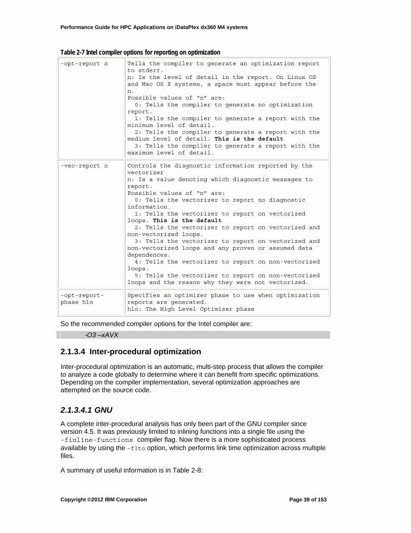
Performance Guide for HPC Applications on iDataPlex dx360 M4 systems
Table 2-7 Intel compiler options for reporting on optimization
-opt-report n Tells the compiler to generate an optimization report to stderr. n: Is the level of detail in the report. On Linux OS and Mac OS X systems, a space must appear before the n. Possible values of “n” are: 0: Tells the compiler to generate no optimization report. 1: Tells the compiler to generate a report with the minimum level of detail. 2: Tells the compiler to generate a report with the medium level of detail. This is the default 3: Tells the compiler to generate a report with the maximum level of detail.
-vec-report n Controls the diagnostic information reported by the vectorizer n: Is a value denoting which diagnostic messages to report. Possible values of “n” are: 0: Tells the vectorizer to report no diagnostic information. 1: Tells the vectorizer to report on vectorized loops. This is the default 2: Tells the vectorizer to report on vectorized and non-vectorized loops. 3: Tells the vectorizer to report on vectorized and non-vectorized loops and any proven or assumed data dependences. 4: Tells the vectorizer to report on non-vectorized loops. 5: Tells the vectorizer to report on non-vectorized loops and the reason why they were not vectorized.
-opt-report-phase hlo
Specifies an optimizer phase to use when optimization reports are generated. hlo: The High Level Optimizer phase
So the recommended compiler options for the Intel compiler are:
-O3 –xAVX
2.1.3.4 Inter-procedural optimization
Inter-procedural optimization is an automatic, multi-step process that allows the compiler to analyze a code globally to determine where it can benefit from specific optimizations. Depending on the compiler implementation, several optimization approaches are attempted on the source code.
2.1.3.4.1 GNU
A complete inter-procedural analysis has only been part of the GNU compiler since version 4.5. It was previously limited to inlining functions into a single file using the -finline-functions compiler flag. Now there is a more sophisticated process available by using the –flto option, which performs link time optimization across multiple files.
A summary of useful information is in Table 2-8:
Copyright ©2012 IBM Corporation
Page 39 of 153
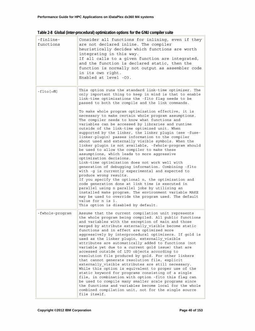
Performance Guide for HPC Applications on iDataPlex dx360 M4 systems
Table 2-8 Global (inter-procedural) optimization options for the GNU compiler suite
-finline-functions
Consider all functions for inlining, even if they are not declared inline. The compiler heuristically decides which functions are worth integrating in this way. If all calls to a given function are integrated, and the function is declared static, then the function is normally not output as assembler code in its own right. Enabled at level -O3.
-flto[=n] This option runs the standard link-time optimizer. The only important thing to keep in mind is that to enable link-time optimizations the -flto flag needs to be passed to both the compile and the link commands. To make whole program optimization effective, it is necessary to make certain whole program assumptions. The compiler needs to know what functions and variables can be accessed by libraries and runtime outside of the link-time optimized unit. When supported by the linker, the linker plugin (see -fuse-linker-plugin) passes information to the compiler about used and externally visible symbols. When the linker plugin is not available, -fwhole-program should be used to allow the compiler to make these assumptions, which leads to more aggressive optimization decisions. Link-time optimization does not work well with generation of debugging information. Combining -flto with -g is currently experimental and expected to produce wrong results. If you specify the optional n, the optimization and code generation done at link time is executed in parallel using n parallel jobs by utilizing an installed make program. The environment variable MAKE may be used to override the program used. The default value for n is 1. This option is disabled by default.
-fwhole-program
Assume that the current compilation unit represents the whole program being compiled. All public functions and variables with the exception of main and those merged by attribute externally_visible become static functions and in effect are optimized more aggressively by interprocedural optimizers. If gold is used as the linker plugin, externally_visible attributes are automatically added to functions (not variable yet due to a current gold issue) that are accessed outside of LTO objects according to resolution file produced by gold. For other linkers that cannot generate resolution file, explicit externally_visible attributes are still necessary. While this option is equivalent to proper use of the static keyword for programs consisting of a single file, in combination with option -flto this flag can be used to compile many smaller scale programs since the functions and variables become local for the whole combined compilation unit, not for the single source file itself.
Copyright ©2012 IBM Corporation
Page 40 of 153

Performance Guide for HPC Applications on iDataPlex dx360 M4 systems
For details and related compiler options, please refer to [15].
2.1.3.4.2 Intel
Intel implementation of Inter Procedural Optimization supports 2 models: single-file compilation using –ip compiler option, and multi-file compilation using –ipo compiler flag.
Optimizations that can be done by Intel compiler when using inter procedural analysis:
Inlining, constant propagation, mod/ref analysis, alias analysis, forward substitution, routine key-attribute propagation, address-taken analysis, partial dead call elimination, symbol table data promotion, common block variable coalescing, dead function elimination, unreferenced variable removal, whole program analysis, array dimension padding, common block splitting, stack frame alignment, structure splitting and field reordering, formal parameter alignment analysis, indirect call conversion, specialization,…
Table 2-9 Global (inter-procedural) optimization options for the Intel compiler suite
-ip This option determines whether additional interprocedural optimizations for single-file compilation are enabled. Options -ip (Linux and Mac OS X) and /Qip (Windows) enable additional interprocedural optimizations for single-file compilation. Options -no-ip may not disable inlining. To ensure that inlining of user-defined functions is disabled, specify -inline-level=0 or -fno-inline.
-ipo
This option enables interprocedural optimization between files. This is also called multifile interprocedural optimization (multifile IPO) or Whole Program Optimization (WPO). When you specify this option, the compiler performs inline function expansion for calls to functions defined in separate files.
-finline-functions
It enables the compiler to perform inline function expansion for calls to functions defined within the current source file.
For details and complete information, please refer to [2].
2.1.3.5 Shared memory parallelization
With the rise of the multi sockets systems and multi core processors, many physical cores are available for a single process to compute its workload. Using shared memory parallelization is the easier way to enable this process to access these multiple computing resources and increase its global performance.
The following techniques allow doing so:
Copyright ©2012 IBM Corporation
Page 41 of 153

Performance Guide for HPC Applications on iDataPlex dx360 M4 systems
Automatic parallelization:
Using a specific compiler option, the user tells the compiler to automatically parallelize the sections that will support it. This parallelization is implemented through shared memory mechanisms and is very similar to OpenMP threading. Parallel execution is managed through environment variables, often the same as are used explicitly with OpenMP.
Explicit parallelization with OpenMP:
In this case, the user inserts directives (or pragmas in C/C++) into the source code telling the compiler which regions need to be parallelized. The user manages the data scope, i.e. which data is shared and which data is private in a thread. Then using compiler options, the compiler transforms the serial code into a multithreaded code. Parallel execution is managed through environment variables from the compiler runtime or OpenMP norm.
Thread Affinity:
Thread affinity is a critical concept when using threads for computing: the locality of the data used by the threads must be managed. The performance of a core will be higher if the data used by the thread running on that core is located in the nearest hardware memory DIMMs. To ensure this locality, one has to bind the thread to run on a particular core, using the data located in the DIMM physically attached to the processor chip containing this core. Environment variables and tools can control this binding. More details are available in Section 3.4.
Compatibility between Intel and GNU:
Intel provides a compatibility library to allow codes compiled with Intel compilers to use the GNU threading mechanisms.
2.1.3.5.1 GNU
Automatic parallelization
The -ftree-parallelize-loops compiler flag creates multithreading automatically:
-ftree-parallelize-loops=n
Parallelize loops, i.e., split the iteration space to run in n threads. This is only possible for loops whose iterations are independent and can be arbitrarily reordered. The optimization is only profitable on multiprocessor machines, for loops that are CPU-intensive, rather than constrained e.g. by memory bandwidth. This option implies –pthread.
This flag must be passed to both the compile and link steps.
OpenMP
The OpenMP directives are processed with the –fopenmp compiler flag.
-fopenmp Enables the OpenMP directives to be recognized by compiler and also arranges for automatic linking of the OpenMP runtime library
Copyright ©2012 IBM Corporation
Page 42 of 153

Performance Guide for HPC Applications on iDataPlex dx360 M4 systems
This flag must be passed to compile and link steps.
When using this flag, all local arrays will be made “automatic” and then allocated on the stack. This can be a source of segmentation faults during execution, because of too small a limit on the stack size. The stack size can be changed by using the following environment variables:
• OMP_STACKSIZE from the OpenMP standard • GOMP_STACKSIZE from the GNU implementation
Both variables change the default size of the stack allocated by each thread.
The size is limited by the value of the stack limit of the user reported by
ulimit –s
Thread affinity
GOMP_CPU_AFFINITY : Binds threads to specific CPUs.
Syntax: GOMP_CPU_AFFINITY="0 3 1-2 4-15:2" will bind the initial thread to CPU 0, the second to CPU 3, the third to CPU 1, the fourth to CPU 2, the fifth to CPU 4, the sixth through tenth to CPUs 6, 8, 10, 12, and 14 respectively and then start assigning back from the beginning of the list.
GOMP_CPU_AFFINITY=0 binds all threads to CPU 0.
OMP_PROC_BIND: Specifies whether threads may be moved between processors. If set to true, OpenMP threads should not be moved, if set to false they may be moved.
2.1.3.5.2 Intel
Automatic parallelization The –parallel compiler flag automatically enables loops to use multithreading. This flag must be passed to both the compile and link steps.
This option must be used with optimization levels -O2 or -O3 (The -O3 option also sets the -opt-matmul flag).
Table 2-10 Automatic parallelization for the Intel compiler
-parallel Tells the auto-parallelizer to generate multithreaded code for loops that can be safely executed in parallel.
Copyright ©2012 IBM Corporation
Page 43 of 153
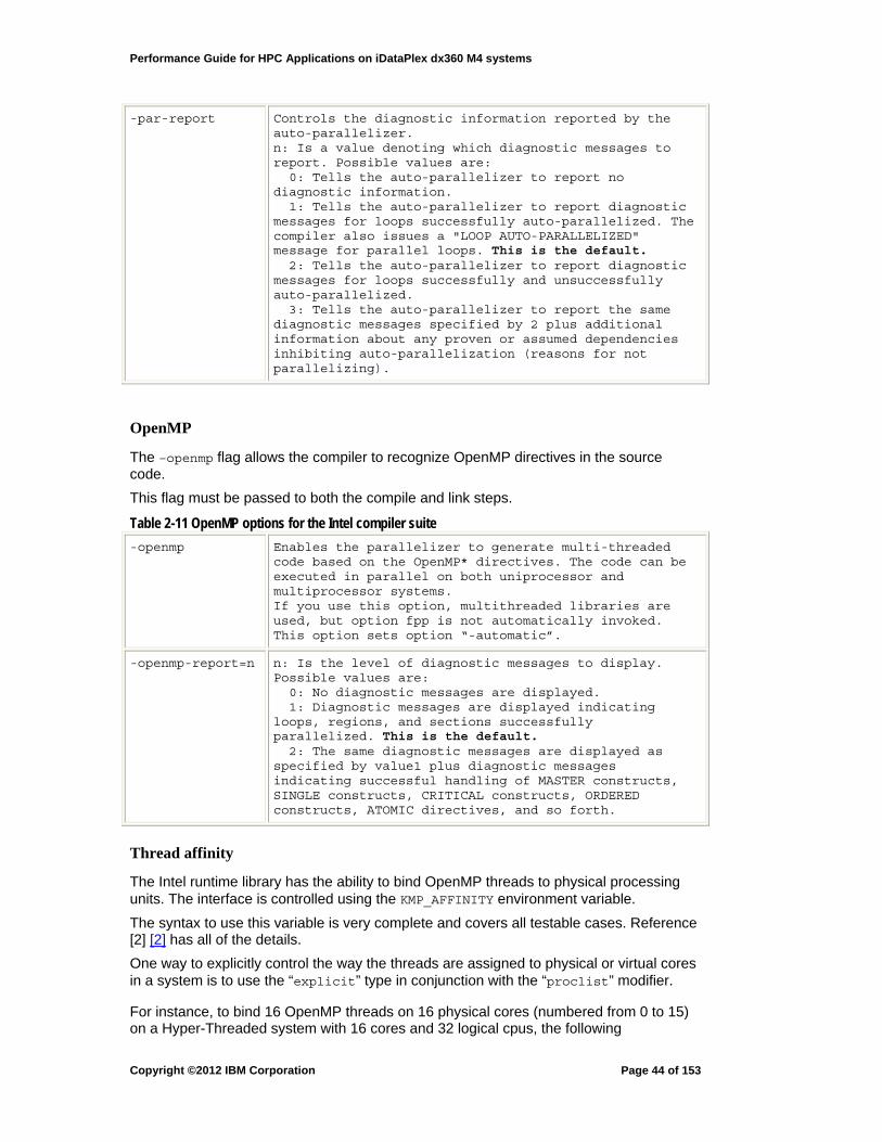
Performance Guide for HPC Applications on iDataPlex dx360 M4 systems
-par-report Controls the diagnostic information reported by the auto-parallelizer. n: Is a value denoting which diagnostic messages to report. Possible values are: 0: Tells the auto-parallelizer to report no diagnostic information. 1: Tells the auto-parallelizer to report diagnostic messages for loops successfully auto-parallelized. The compiler also issues a "LOOP AUTO-PARALLELIZED" message for parallel loops. This is the default. 2: Tells the auto-parallelizer to report diagnostic messages for loops successfully and unsuccessfully auto-parallelized. 3: Tells the auto-parallelizer to report the same diagnostic messages specified by 2 plus additional information about any proven or assumed dependencies inhibiting auto-parallelization (reasons for not parallelizing).
OpenMP
The –openmp flag allows the compiler to recognize OpenMP directives in the source code.
This flag must be passed to both the compile and link steps.
Table 2-11 OpenMP options for the Intel compiler suite
-openmp Enables the parallelizer to generate multi-threaded code based on the OpenMP* directives. The code can be executed in parallel on both uniprocessor and multiprocessor systems. If you use this option, multithreaded libraries are used, but option fpp is not automatically invoked. This option sets option “-automatic”.
-openmp-report=n n: Is the level of diagnostic messages to display. Possible values are: 0: No diagnostic messages are displayed. 1: Diagnostic messages are displayed indicating loops, regions, and sections successfully parallelized. This is the default. 2: The same diagnostic messages are displayed as specified by value1 plus diagnostic messages indicating successful handling of MASTER constructs, SINGLE constructs, CRITICAL constructs, ORDERED constructs, ATOMIC directives, and so forth.
Thread affinity
The Intel runtime library has the ability to bind OpenMP threads to physical processing units. The interface is controlled using the KMP_AFFINITY environment variable.
The syntax to use this variable is very complete and covers all testable cases. Reference [2] [2] has all of the details.
One way to explicitly control the way the threads are assigned to physical or virtual cores in a system is to use the “explicit” type in conjunction with the “proclist” modifier.
For instance, to bind 16 OpenMP threads on 16 physical cores (numbered from 0 to 15) on a Hyper-Threaded system with 16 cores and 32 logical cpus, the following
Copyright ©2012 IBM Corporation
Page 44 of 153
Performance Guide for HPC Applications on iDataPlex dx360 M4 systems
environment settings are equivalent:
export OMP_NUM_THREADS=16 export KMP_AFFINITY="proclist=[0-15:1],granularity=fine,explicit” export KMP_AFFINITY= \ "proclist=[0,1,2,3,4,5,6,7,8,9,10,11,12,13,14,15],granularity=fine,explicit"
Compatibility between Intel and GNU
Intel provides a way to recognize the GNU syntax for the OpenMP runtime environment with Intel compilers. These environment variables are GNU extensions. They are recognized by the Intel OpenMP compatibility library.
Table 2-12 GNU OpenMP runtime environment variables recognized by the Intel compiler toolchain
GOMP_STACKSIZE GNU extension recognized by the Intel OpenMP compatibility library. Same as OMP_STACKSIZE. KMP_STACKSIZE overrides GOMP_STACKSIZE, which overrides OMP_STACKSIZE.
GOMP_CPU_AFFINITY GNU extension recognized by the Intel OpenMP compatibility library. Specifies a list of OS processor IDs. Default: Affinity is disabled
Add the compiler option
-openmp-lib compat
to use these environment variables to manage an OpenMP job.
GOMP_CPU_AFFINITY and KMP_AFFINITY with the “explicit” type have the same syntax.
The following 3 statements are equivalent:
export GOMP_CPU_AFFINITY="0,1,2,3,4,5,6,7,8,9,10,11,12,13,14,15” export GOMP_CPU_AFFINITY="0-15:1” export KMP_AFFINITY="proclist=[0-15:1],granularity=fine,explicit”
2.1.3.6 Distributed memory parallelization
In order to use a cluster of systems, one has to choose a method that can address the issue of synchronizing distributed memory used by a simple program. The most popular method is to use the Message Passing Interface (MPI) API, which enables processes to share information by exchanging messages.
Recently, Coarrays have emerged as an alternative method integrated into the Fortran compiler and may be a future contender to address distributed parallelism. Coarrays (also called CAF = Co Array Fortran) allow parallel programs to use a Partitioned Global Address Space (PGAS) following the SPMD (single program, multiple data) parallelization paradigm. Each process (called an image) has its own private variables. Variables which have a so-called codimension are addressable from other images. This extension is part of the Fortran 2008 standard.
Copyright ©2012 IBM Corporation
Page 45 of 153
Performance Guide for HPC Applications on iDataPlex dx360 M4 systems
Various compilers implement Coarrays but do not have the same functionality.
2.1.3.6.1 GNU
The implementation of CAF in the GNU Fortran compiler is very new and almost useless. The latest information and status are available at http://gcc.gnu.org/wiki/Coarray and http://gcc.gnu.org/wiki/CoarrayLib.
Reported from the “Current Implementation Status in GCC Fortran on the GCC Trunk [4.7 (experimental)]”
• GCC 4.6: Only single-image support (i.e. num_images() == 1) but many features do not work.
• GCC 4.7: Includes multi-image support via a communication library. There is comprehensive support for a single image, but most features do not yet work with num_images() > 1.
To enable a Fortran code to use CAF with the GNU compiler, the user has to specify the -fcoarray switch:
Table 2-13 GNU compiler options for CAF
-fcoarray= <keyword>
keyword= none: Disable coarray support; using coarray declarations and image-control statements will produce a compile-time error. (Default) single: Single-image mode, i.e. num_images() is always one. lib: Library-based coarray parallelization; a suitable GNU Fortran coarray library needs to be linked. Single-image, MPI, ARMCI communication libraries are under development.
2.1.3.6.2 Intel
The CAF implementation in the Intel compiler is more mature and allows compiling and running with coarrays on local and remote nodes. It uses shared memory transfers for intra-node accesses/transfers and Intel MPI for inter-node exchanges. No comparison of the CAF implementation and the native MPI implementation has been done.
The compiler option -coarray must be included to enable coarrays in a program.
Table 2-14 Intel compiler options for CAF
-coarray [=shared|distributed]
Enable coarray syntax for data parallel programming. The default is shared-memory; distributed memory is only valid with the Intel Cluster Toolkit license.
-coarray-num-images=n Set the default number of coarray images. Note that when a setting is specified in the environment variable FOR_COARRAY_NUM_IMAGES, it overrides the compiler option setting.
2.1.4 Alternatives
The following compiler suites include FORTRAN, C, and C++ compilers supporting the Intel Sandy Bridge features and provide also tools for debugging, optimization, auto parallelization, etc. They have not been assessed recently enough to be included in this
Copyright ©2012 IBM Corporation
Page 46 of 153
Performance Guide for HPC Applications on iDataPlex dx360 M4 systems
document.
• The PGI Workstation compilers from the Portland Group [11] • The PathScale EKOPath 4 compilers from PathScale [10]
2.2 Libraries
HPC libraries are fundamental tools for scientists during code development: They provide standardized interfaces to tested implementations of algorithms, methods, and solvers. They are easy to use and more efficient than manually coding the equivalent functionality. Frequently, they are already vectorized and parallelized to take advantage of modern HPC architectures.
HPC codes are usually developed following open standards for the libraries, but used in production with highly optimized math libraries like MKL for Intel processors.
2.2.1 Intel® Math Kernel Library (MKL)
The MKL library is provided by Intel and contains various mathematical routines highly optimized for Intel Sandy Bridge processors.
2.2.1.1 Linear Algebra and Solvers
Functions calls from BLAS, LAPACK and ScaLAPACK1 libraries are automatically replaced by functions from MKL if you are linking with MKL library (see Section 2.2.1.5 for the correct linking syntax). Serial, multi threaded (OpenMP) and distributed (MPI) versions of these routines are available when possible.
Sparse BLAS and solvers are also available in MKL library. It supports CSR, CSC, BSR, DIA and Skyline data storage as well as NIST and SparseKit style interfaces.
2.2.1.2 Fast Fourier Transform
Codes already implementing the Fast Fourier Transforms using the FFTW implementation can quickly benefit from Intel MKL performance by using the wrappers included in MKL package [7]. Serial, multi threaded (OpenMP) and distributed (MPI) versions of these routines are available when possible.
2.2.1.3 Vector Math Library (VML)
The Vector Math Library (VML) [8] is designed to compute elementary functions on vector arguments. VML is an integral part of the Intel MKL library and includes a set of highly optimized implementations of certain computationally expensive core mathematical functions (power, trigonometric, exponential, hyperbolic, etc.) that operate on vectors. VML may improve performance for such applications as nonlinear software, computations of integrals, and many others.
2.2.1.4 Vector Statistical Library (VSL)
Vector Statistical Library (VSL) [9] performs pseudorandom and quasi-random vector generation as well as convolution and correlation mathematical operations. VSL is an
Copyright ©2012 IBM Corporation
Page 47 of 153
Performance Guide for HPC Applications on iDataPlex dx360 M4 systems
integral part of MKL library and provides a number of generator subroutines implementing commonly used continuous and discrete distributions to help improve their performance. All these distributions are based on the highly optimized Basic Random Number Generators (BRNGs) and VML.
2.2.1.5 How is the MKL library used?
A very useful tool is the “Intel Math Kernel Library Link Line Advisor” [6]. Given the configuration of the libraries to be used, it provides the exact syntax to be passed to compiler and linker in order to correctly link the MKL libraries and their dependencies.
For instance, for the following configuration: Linux + Intel Fortran compiler + SMP version of MKL + SCALAPACK + BLACS + Fortran95 interface for BLAS and LAPACK, this tool provides the following information:
Compiler options:
-I$(MKLROOT)/include/intel64/lp64 -I$(MKLROOT)/include
For the link line:
-L$(MKLROOT)/lib/intel64 $(MKLROOT)/lib/intel64/libmkl_blas95_lp64.a (MKLROOT)/lib/intel64/libmkl_lapack95_lp64.a -lmkl_scalapack_lp64 -lmkl_intel_lp64 -lmkl_intel_thread -lmkl_core -lmkl_blacs_intelmpi_lp64 -openmp -lpthread –lm
The GNU compiler, MPICH, 32bit and 64bit are some of the possibilities to use with the MKL library.
2.2.2 Alternative Libraries
Many alternative libraries to MKL exist, most of them being open source or freely available. Some of the libraries widely adopted by HPC community are introduced below.
2.2.2.1 BLAS
The BLAS (Basic Linear Algebra Subprograms) [16] are routines that provide standard building blocks for performing basic vector and matrix operations. The Level 1 BLAS perform scalar, vector and vector-vector operations, the Level 2 BLAS perform matrix-vector operations, and the Level 3 BLAS perform matrix-matrix operations. Because the BLAS are efficient, portable, and widely available, they are commonly used in the development of high quality linear algebra software, LAPACK for example.
2.2.2.2 LAPACK
LAPACK [17] is written in Fortran 90 and provides routines for solving systems of simultaneous linear equations, least-squares solutions of linear systems of equations, eigenvalue problems, and singular value problems. The associated matrix factorizations (LU, Cholesky, QR, SVD, Schur, and generalized Schur) are also provided, as are related computations such as reordering of the Schur factorizations and estimating condition numbers. Dense and banded matrices are handled, but not general sparse matrices. In all areas, similar functionality is provided for real and complex matrices, in both single and double precision.
Copyright ©2012 IBM Corporation
Page 48 of 153

Performance Guide for HPC Applications on iDataPlex dx360 M4 systems
2.2.2.3 SCALAPACK
The ScaLAPACK [18] (or Scalable LAPACK) library includes a subset of LAPACK routines redesigned for distributed memory MIMD parallel computers. It is currently written in a Single-Program-Multiple-Data style using explicit message passing for inter processor communication. It assumes matrices are laid out in a two-dimensional block cyclic decomposition.
ScaLAPACK is designed for heterogeneous computing and is portable on any computer that supports MPI.
2.2.2.4 ATLAS
The ATLAS [19] (Automatically Tuned Linear Algebra Software) project is an ongoing research effort focusing on applying empirical techniques in order to provide portable performance. At present, it provides C and Fortran77 interfaces to a portably efficient BLAS implementation, as well as a few routines from LAPACK.
2.2.2.5
2.2.2.6 FFTW
FFTW [20] is a C subroutine library for computing the discrete Fourier transform (DFT) in one or more dimensions, of arbitrary input size, and of both real and complex data (as well as of even/odd data, i.e. the discrete cosine/sine transforms or DCT/DST).
The latest official release of FFTW is version 3.3.1 and introduces support for the AVX x86 extensions.
2.2.2.7 GSL
The GNU Scientific Library (GSL) [21] is a numerical library for C and C++ programmers. It is free software under the GNU General Public License.
The library provides a wide range of mathematical routines such as random number generators, special functions and least-squares fitting. There are over 1000 functions in total with an extensive test suite.
2.3 References
All of the descriptions of the GNU and Intel compiler options included in the tables in this chapter are taken from the GNU Optimization Options Guide and the Intel Fortran Compiler User and Reference Guide.
[1] Intel Composer XE web page: http://software.intel.com/en-us/articles/intel-composer-xe/ [2] Intel Fortran Compiler User and Reference guide :
http://software.intel.com/sites/products/documentation/hpc/composerxe/en-us/2011Update/fortran/lin/index.htm
[3] Intel AVX web page: http://software.intel.com/en-us/avx/ [4] Intel MKL: web page: http://software.intel.com/en-us/articles/intel-mkl/
Copyright ©2012 IBM Corporation
Page 49 of 153
Performance Guide for HPC Applications on iDataPlex dx360 M4 systems
[5] Intel MKL in depth: http://www.cs-software.com/software/fortran/intel/mkl_indepth.pdf [6] Intel MKL Link Line Advisor: http://software.intel.com/en-us/articles/intel-mkl-link-line-
advisor/ [7] Intel MKL: FFTW to MKL: http://software.intel.com/en-us/articles/the-intel-math-kernel-
library-and-its-fast-fourier-transform-routines/ [8] Intel MKL : VML library:
http://software.intel.com/sites/products/documentation/hpc/mkl/vml/vmldata.htm [9] Intel MKL : VSL library :
http://software.intel.com/sites/products/documentation/hpc/mkl/vslnotes/index.htm and http://software.intel.com/sites/products/documentation/hpc/mkl/sslnotes/index.htm
[10] PathScale Compilers web site: http://www.pathscale.com/ekopath.html [11] PGI Compilers web site: http://www.pgroup.com/ [12] GNU Compilers web site: http://www.gnu.org/software/gcc/ [13] GNU gfortran web page: http://gcc.gnu.org/fortran/ [14] GNU Online Documentation: http://gcc.gnu.org/onlinedocs/ [15] GNU Optimization Options guide : http://gcc.gnu.org/onlinedocs/gcc/Optimize-
Options.html [16] BLAS Library web site: http://www.netlib.org/blas/index.html [17] LAPACK Library web site: http://www.netlib.org/lapack/ [18] SCALAPACK Library web site: http://www.netlib.org/scalapack/ [19] ATLAS library web site: http://math-atlas.sourceforge.net/ [20] FFTW library web site: http://www.fftw.org/ [21] GSL library web site: http://www.gnu.org/software/gsl/
Copyright ©2012 IBM Corporation
Page 50 of 153

Performance Guide for HPC Applications on iDataPlex dx360 M4 systems
3 Linux
The iDataPlex dx360 M4 supports the following versions of 64bit (x86-64) Red Hat Enterprise Linux (RHEL) and SUSE Enterprise Linux Server (SLES):
• SLES 10.4 with Xen • SLES 11.2 with KVM or Xen • RHEL 5.7 with KVM or Xen • RHEL 6.2 with KVM
3.1 Core Frequency Modes
Linux fully supports the clock frequency scaling capabilities of the Intel processors available in the dx360 M4. Both Enhanced Intel Speedstep® Technology (EIST) and Turbo Boost are fully supported. These features allow the core clock frequency to be dynamically adjusted to achieve the desired blend of performance and energy management.
The processor frequency settings can be controlled through either hardware or software. The hardware configuration is controllable through the system's UEFI interface which is available during system initialization. It is also possible to adjust the UEFI configuration using the IBM Advanced Settings Utility (ASU). Detailed information on ASU is available in section 1.2.3.1.
In addition to the available hardware controls, Linux provides its own clock frequency management. Linux uses what are referred to as CPU “governors” to manage clock frequency. The two most common governors are performance and ondemand. The performance governor always runs the processor at its nominal clock frequency. In contrast, the ondemand governor will vary the clock frequency depending on the processor utilization levels of the system. The method of controlling the clock frequency management in Linux varies from one distribution to the next, so it is best to consult the distribution documentation for details.
• RHEL 6 • SLES 11
More information is included in the cpufrequtils packages available on RHEL and SLES. To find the exact package needed on RHEL, try
$ yum search cpufreq
On SLES, try
$ zypper search cpufreq
3.2 Memory Page Sizes
The Linux memory page size support varies from one hardware architecture to the next. On x86-64 there are only two supported page sizes: 4 KB and 2 MB. The 4 KB page size is considered the default, while the 2 MB page size is what is referred to as a huge page.
Using the 2 MB huge page can improve performance by reducing pressure on the processor's translation lookaside buffer (TLB) which typically has a fixed number of elements that it can cache. By increasing the page size, the TLB is capable of caching entries that address larger amounts of memory than when small pages are used. Historically access to the 2 MB page size has been restricted to applications specifically
Copyright ©2012 IBM Corporation
Page 51 of 153

Performance Guide for HPC Applications on iDataPlex dx360 M4 systems
coded to do so which has limited the ability to make use of this feature.
Two recent additions to Linux have increased the viability of using huge pages for applications without specifically modifying them to do so. The libhugetlbfs project enables applications to explicitly make use of huge pages when the user requests them. There are usability concerns with libhugetlbfs since the huge pages must be allocated ahead of time by the system administrator. This is done using the following command (allocating 30 huge pages in this case):
# echo 30 > /proc/sys/vm/nr_hugepages
In order for huge pages to be allocated in this manner, the operating system must be able to find appropriately sized regions of contiguous free memory (2 MB in this case). This can be problematic on systems which have been running for awhile, where memory fragmentation has occurred.
The number of allocated pages (and current usage) can be checked by running the following command:
# grep HugePage /proc/meminfo AnonHugePages: 4237312 kB HugePages_Total: 30 HugePages_Free: 30 HugePages_Rsvd: 0 HugePages_Surp: 0
As shown in this output (line AnonHugePages), recent x86-64 Linux distributions (including RHEL 6.2 and SLES 11.2) support a new kernel feature called transparent huge pages (THP). This example shows over 4 GB of memory backed by huge pages allocated via THP. THP allows for applications to automatically be backed by huge pages without any special effort by the user. To enable THP, the Linux memory management subsystem has been enhanced with a memory defragmenter. The defragmenter increases the likelihood of large contiguous memory regions being available after the system has been running for awhile. The presence of THP does not preclude the use of explicit huge pages or libhugetlbfs. The presence of the new memory defragmenter should make their use easier.
3.3 Memory Affinity
3.3.1 Introduction
Linux optimizes for memory access performance by attempting to make memory allocations in a NUMA (Non Uniform Memory Access) aware fashion. That is, Linux will attempt to allocate local memory when possible and only resort to performing a remote allocation if the local allocation fails.
While the allocation path attempts to behave in an optimal fashion, this behavior can be offset by the kernel's task scheduler, which is not NUMA aware. It is possible (likely even) that the task scheduler can move a process / thread to a core which is remote to the already allocated memory. This increases the memory access latency and may decrease the achievable memory bandwidth. This is one reason why it is recommended that most HPC applications perform explicit process or thread binding.
3.3.2 Using numactl
While Linux attempts to optimally allocate memory by default, it may be useful to explicitly control the allocation behavior in some scenarios. The numactl command is one
Copyright ©2012 IBM Corporation
Page 52 of 153

Performance Guide for HPC Applications on iDataPlex dx360 M4 systems
method of doing so.
To display the NUMA topology (memory and processor topology) on the dx360 M4:
% numactl --hardware
The output should be similar to the following, depending on the installed processors and memory:
% numactl --hardware available: 2 nodes (0-1) node 0 cpus: 0 1 2 3 4 5 6 7 16 17 18 19 20 21 22 23 node 0 size: 65514 MB node 0 free: 61196 MB node 1 cpus: 8 9 10 11 12 13 14 15 24 25 26 27 28 29 30 31 node 1 size: 65536 MB node 1 free: 56252 MB node distances: node 0 1 0: 10 11 1: 11 10
The numactl utility can be used to modify memory allocation in a variety of manners such as:
Require allocation on a specific NUMA node(s) Prefer allocation on a specific NUMA node(s) Interleave allocation on specific NUMA nodes
Interleaving is particularly useful when memory allocation is performed by a master thread and application source code modification is not possible.
For further information, and detailed command argument documentation, man numactl.
3.4 Process and Thread Binding
3.4.1 taskset
taskset is the Linux system command that:
• sets the processor affinity of a running process • sets the processor affinity when launching a new command • retrieves the processor affinity of a running process
As such, taskset is a low-level mechanism for managing processor affinity.
Practically speaking, the typical usages of the taskset command are the following:
• At process startup: set processor affinity while launching a new command
% taskset -c <cpu list> <command>
• During execution: retrieve processor affinity of a running process
% taskset -cp <process ID>
In the context of an MPI parallel execution, the ‘taskset’ command must be integrated into a user-defined script that will be responsible for performing an automatic mapping
Copyright ©2012 IBM Corporation
Page 53 of 153

Performance Guide for HPC Applications on iDataPlex dx360 M4 systems
between a given MPI rank and a unique processor ID for each process instance.
A typical example of such a user-defined script is provided below for reference:
#!/bin/bash # Read user-defined parameters for process affinity configuration STRIDE=1 OFFSET=0 # Retrieve number of processors on the node export PROCESSORS=$(grep "^processor" /proc/cpuinfo | wc -l) # Retrieve MPI rank for given process depending on selected MPI library # Open MPI if [ -n "$OMPI_COMM_WORLD_RANK" ]; then MPI_RANK=$OMPI_COMM_WORLD_RANK # Intel MPI elif [ -n "$PMI_RANK" ]; then MPI_RANK=$PMI_RANK else echo "Error getting MPI rank for process - Aborting…"; exit 1 fi # Compute processor ID to bind the process to CPU=$MPI_RANK CPU=$(( $CPU * $STRIDE )) CPU=$(( $CPU + $OFFSET )) CPU=$(( $CPU % $PROCESSORS )) # Launch command with taskset prefix CMD="taskset -c $CPU $@"
The affinity management script above must be used as a prefix for the application binary in the ‘mpirun’ submission command:
% mpirun -np <# tasks> <affinity management> <binary> <arguments>
A comprehensive reference for the ‘taskset’ command can be found here.
3.4.2 numactl
numactl is the Linux system command that allows processes to run with a specific NUMA scheduling or memory placement policy. Its coverage is broader than the one of the ‘taskset’ system command as it also manages the memory placement for a process.
The typical usages of the numactl command are the following:
• Display NUMA configuration of the node, including socket / core / memory components:
% numactl --hardware available: 2 nodes (0-1) node 0 cpus: 0 1 2 3 4 5 12 13 14 15 16 17 node 0 size: 12276 MB node 0 free: 10686 MB node 1 cpus: 6 7 8 9 10 11 18 19 20 21 22 23 node 1 size: 12288 MB node 1 free: 10896 MB node distances: node 0 1 0: 10 21 1: 21 10
• Set explicit processor affinity while launching a new process:
Copyright ©2012 IBM Corporation
Page 54 of 153

Performance Guide for HPC Applications on iDataPlex dx360 M4 systems
% numactl --physcpubind=0-3,6-11 <binary> <arguments>
• Set explicit memory affinity while launching a new process:
% numactl --membind=0 <binary> <arguments>
A comprehensive reference for the ‘numactl’ command can be found here.
In the context of an MPI parallel execution, as is the case with the ‘taskset’ command, the ‘numactl’ command must be integrated into a user-defined script that is to be responsible for performing an automatic mapping between a given MPI rank and a unique processor ID for each process instance.
3.4.3 Environment Variables for OpenMP Threads
Processor affinity management for OpenMP threads can be controlled by different environment variables depending on the compilation/runtime environment.
GNU The environment variable GOMP_CPU_AFFINITY is used to specify an explicit binding for OpenMP threads.
Intel
The Intel compilers’ OpenMP runtime library provides the Intel OpenMP Thread Affinity Interface, which is made up of three levels:
1. High-level affinity interface this interface is entirely controlled by one single environment variable (KMP_AFFINITY), which is used to determine the machine topology and to assign OpenMP threads to the processors based upon their physical location in the machine.
2. Mid-level affinity interface
this interface provides compatibility with the GNU GOMP_CPU_AFFINITY environment variable, but it can be invoked as well by using the KMP_AFFINITY environment variable. • GOMP_CPU_AFFINITY
Using the GOMP_CPU_AFFINITY environment variable requires specifying the following compile option: ‘-openmp-lib compat’
• KMP_AFFINITY The explicit binding of OpenMP threads can be specified.
3. Low-level affinity interface (not discussed in the present document)
This interface uses APIs to enable OpenMP threads to make calls into the OpenMP runtime library to explicitly specify the set of processors on which they are to be run.
The GOMP_CPU_AFFINITY environment variable expects a comma-separated list composed of the following elements:
• single processor ID • a range of processor IDs (M-N) • a range of processor IDs with some stride (M-N:S)
The KMP_AFFINITY environment variable expects the following syntax:
KMP_AFFINITY=[<modifier>,]<type>
Copyright ©2012 IBM Corporation
Page 55 of 153
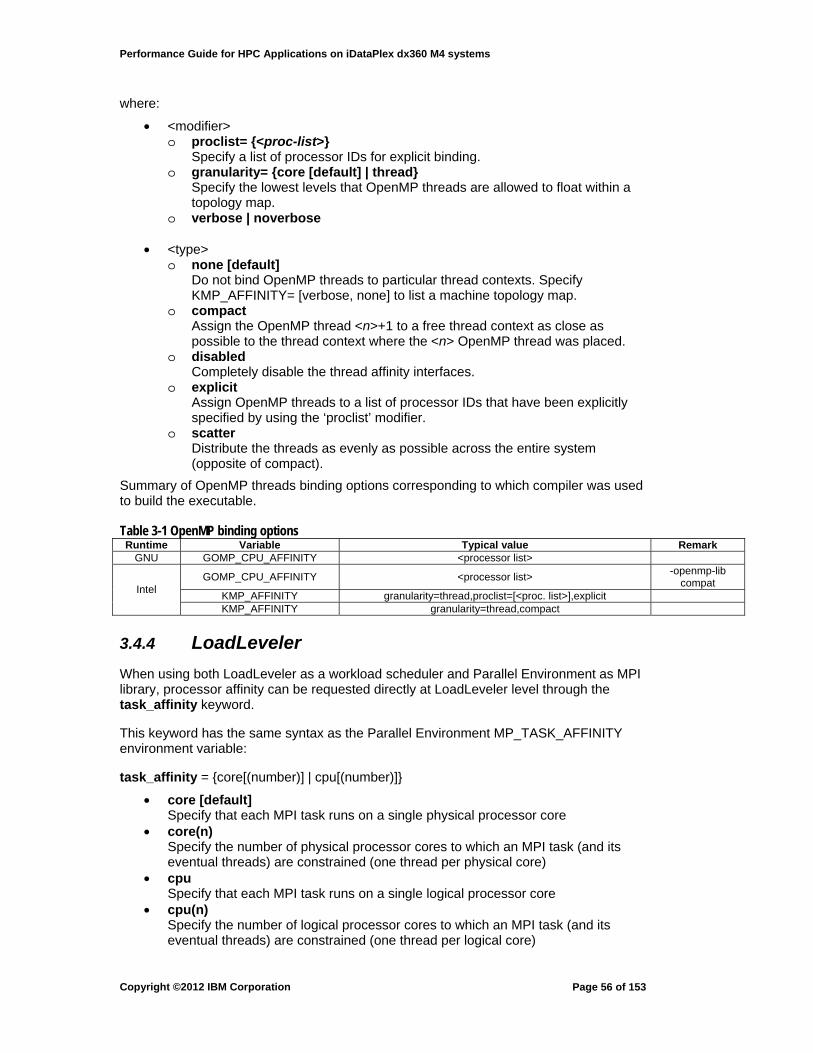
Performance Guide for HPC Applications on iDataPlex dx360 M4 systems
where:
• <modifier> o proclist= {<proc-list>}
Specify a list of processor IDs for explicit binding. o granularity= {core [default] | thread}
Specify the lowest levels that OpenMP threads are allowed to float within a topology map.
o verbose | noverbose
• <type> o none [default]
Do not bind OpenMP threads to particular thread contexts. Specify KMP_AFFINITY= [verbose, none] to list a machine topology map.
o compact Assign the OpenMP thread <n>+1 to a free thread context as close as possible to the thread context where the <n> OpenMP thread was placed.
o disabled Completely disable the thread affinity interfaces.
o explicit Assign OpenMP threads to a list of processor IDs that have been explicitly specified by using the ‘proclist’ modifier.
o scatter Distribute the threads as evenly as possible across the entire system (opposite of compact).
Summary of OpenMP threads binding options corresponding to which compiler was used to build the executable.
Table 3-1 OpenMP binding options Runtime Variable Typical value Remark
GNU GOMP_CPU_AFFINITY <processor list>
GOMP_CPU_AFFINITY <processor list> -openmp-lib
compat KMP_AFFINITY granularity=thread,proclist=[<proc. list>],explicit
Intel
KMP_AFFINITY granularity=thread,compact
3.4.4 LoadLeveler
When using both LoadLeveler as a workload scheduler and Parallel Environment as MPI library, processor affinity can be requested directly at LoadLeveler level through the task_affinity keyword.
This keyword has the same syntax as the Parallel Environment MP_TASK_AFFINITY environment variable:
task_affinity = {core[(number)] | cpu[(number)]}
• core [default] Specify that each MPI task runs on a single physical processor core
• core(n) Specify the number of physical processor cores to which an MPI task (and its eventual threads) are constrained (one thread per physical core)
• cpu Specify that each MPI task runs on a single logical processor core
• cpu(n) Specify the number of logical processor cores to which an MPI task (and its eventual threads) are constrained (one thread per logical core)
Copyright ©2012 IBM Corporation
Page 56 of 153
Performance Guide for HPC Applications on iDataPlex dx360 M4 systems
The following two additional keywords complement the task_affinity keyword:
• cpus_per_core = <number> Specify the number of logical cores per physical processor core that needs to be allocated to each task of a job with the processor-core affinity requirement. This keyword can only be used along with the task_affinity keyword.
• parallel_threads = <number> Request OpenMP thread-level binding by assigning separate logical cores to individual threads of an OpenMP task. LoadLeveler uses the ‘parallel_threads’ value to set the value for the OMP_NUM_THREADS runtime environment variable for all job types. For serial jobs, LoadLeveler also uses the ‘parallel_threads’ value to set the GOMP_CPU_AFFINITY / KMP_AFFINITY environment variables.
3.5 Hyper-Threading (HT) Management
Hyper-Threading (HT) or simultaneous multithreading (SMT) is a processor feature that allows multiple threads of execution to exist on a processor core at the same time. The individual execution threads share access to the processor's functional units, allowing multiple units to be used simultaneously which often increases efficiency. When running traditional business logic applications, the effects of HT / SMT are almost always positive. However, this is not always the case for HPC applications.
In order to experiment with the effects of HT / SMT it must be enabled or disabled through a hardware configuration change. This can be accomplished during system initialization by entering the UEFI control interface or by using the ASU utility presented in Section 1.2.3.1. To enable or disable HT / SMT using the ASU, run the following command:
# asu64 set Processors.Hyper-Threading <Enable|Disable>
Then, a system reboot will activate the changes to the HT / SMT configuration. Depending on whether HT / SMT is being enabled or disabled, the number of processors visible to Linux should either double or be cut in half.
The CPU Hotplug method
An alternative approach (which is more flexible, but also more elaborate) is to use the CPU hotplug method to turn on or off individual CPUs. This method uses commands like
echo 0 > /sys/devices/system/cpu/cpu16/online
to disable, and
echo 1 > /sys/devices/system/cpu/cpu16/online
to enable specific CPUs. But, to be truly effective, the mapping between logical CPUs and physical cores in the system need to be known in advance, and the finer points of implementing this robustly are outside the scope of this document.
3.6 Hardware Prefetch Control
Modifying the hardware prefetch controls of the dx360 M4 changes the behavior of the processor with respect to pulling data from main memory into the processor's cache. For memory access sensitive applications, which many HPC applications are, these settings may provide valuable performance gains with the proper configuration.
These settings are low level hardware configuration details that are not normally visible from within Linux. Modification of these controls can be accomplished during system
Copyright ©2012 IBM Corporation
Page 57 of 153

Performance Guide for HPC Applications on iDataPlex dx360 M4 systems
initialization by entering the UEFI control interface or by using the ASU utility presented in Section 1.2.3.1. To see what prefetch controls can be modified, run the following command:
# asu64 show all | grep Prefetch Processors.HardwarePrefetcher=Enable Processors.AdjacentCachePrefetch=Enable Processors.DCUStreamerPrefetcher=Disable Processors.DCUIPPrefetcher=Enable
Each of these controls can be modified using the following ASU syntax:
# asu64 set <property> <Enable|Disable>
For example:
# asu64 set Processors.HardwarePrefetcher Disable
To activate changes to the prefetch controls a system reboot is required. Since these properties are not normally visible from Linux, verifying the current settings requires the use of ASU.
3.7 Monitoring Tools for Linux
Below is a brief overview of select monitoring tools that exist on systems running Linux. Unless otherwise noted, the output provided is exemplary of the default operating modes of these utilities. The man pages for these utilities give in depth descriptions of the programs and of the many optional parameters that each has.
It is recommended to ignore the first sample of data from many of these utilities since that data point represents an average of all data collected since the system was booted instead of the previous interval.
3.7.1 Top
The top utility is a universally available Linux utility for monitoring the state of individual processes and the system as a whole. It is primarily a tool used to focus on CPU utilization and memory consumption but it does expose additional information such as scheduler priorities and page fault statistics.
Typical output:
# top top - 15:09:46 up 55 min, 6 users, load average: 0.04, 0.01, 0.00 Tasks: 397 total, 1 running, 396 sleeping, 0 stopped, 0 zombie Cpu(s): 0.0%us, 0.0%sy, 0.0%ni,100.0%id, 0.0%wa, 0.0%hi, 0.0%si, 0.0%st Mem: 24596592k total, 602736k used, 23993856k free, 24112k buffers Swap: 26836984k total, 0k used, 26836984k free, 135456k cached PID USER PR NI VIRT RES SHR S %CPU %MEM TIME+ COMMAND 1 root 20 0 19396 1572 1264 S 0.0 0.0 0:01.00 init 2 root 20 0 0 0 0 S 0.0 0.0 0:00.00 kthreadd 3 root RT 0 0 0 0 S 0.0 0.0 0:00.00 migration/0 4 root 20 0 0 0 0 S 0.0 0.0 0:00.00 ksoftirqd/0 5 root RT 0 0 0 0 S 0.0 0.0 0:00.00 migration/0
Copyright ©2012 IBM Corporation
Page 58 of 153
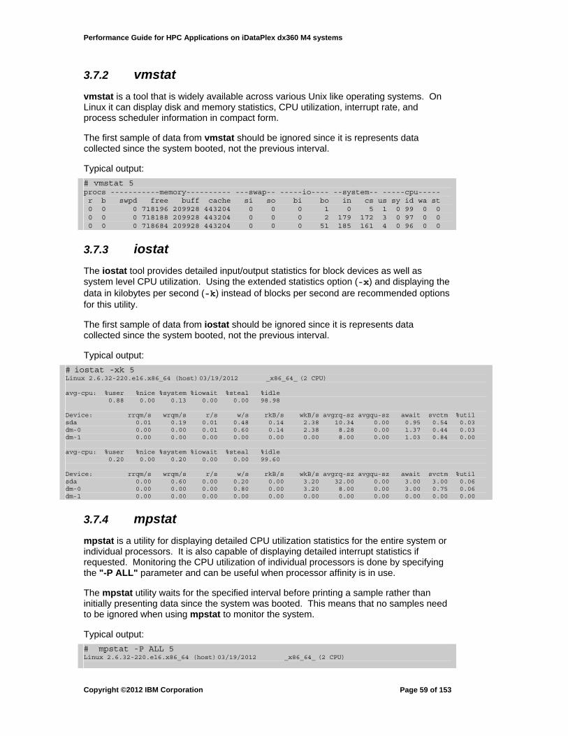
Performance Guide for HPC Applications on iDataPlex dx360 M4 systems
3.7.2 vmstat
vmstat is a tool that is widely available across various Unix like operating systems. On Linux it can display disk and memory statistics, CPU utilization, interrupt rate, and process scheduler information in compact form.
The first sample of data from vmstat should be ignored since it is represents data collected since the system booted, not the previous interval.
Typical output:
# vmstat 5 procs -----------memory---------- ---swap-- -----io---- --system-- -----cpu----- r b swpd free buff cache si so bi bo in cs us sy id wa st 0 0 0 718196 209928 443204 0 0 0 1 0 5 1 0 99 0 0 0 0 0 718188 209928 443204 0 0 0 2 179 172 3 0 97 0 0 0 0 0 718684 209928 443204 0 0 0 51 185 161 4 0 96 0 0
3.7.3 iostat
The iostat tool provides detailed input/output statistics for block devices as well as system level CPU utilization. Using the extended statistics option (-x) and displaying the data in kilobytes per second (-k) instead of blocks per second are recommended options for this utility.
The first sample of data from iostat should be ignored since it is represents data collected since the system booted, not the previous interval.
Typical output:
# iostat -xk 5 Linux 2.6.32-220.el6.x86_64 (host) 03/19/2012 _x86_64_ (2 CPU) avg-cpu: %user %nice %system %iowait %steal %idle 0.88 0.00 0.13 0.00 0.00 98.98 Device: rrqm/s wrqm/s r/s w/s rkB/s wkB/s avgrq-sz avgqu-sz await svctm %util sda 0.01 0.19 0.01 0.48 0.14 2.38 10.34 0.00 0.95 0.54 0.03 dm-0 0.00 0.00 0.01 0.60 0.14 2.38 8.28 0.00 1.37 0.44 0.03 dm-1 0.00 0.00 0.00 0.00 0.00 0.00 8.00 0.00 1.03 0.84 0.00 avg-cpu: %user %nice %system %iowait %steal %idle 0.20 0.00 0.20 0.00 0.00 99.60 Device: rrqm/s wrqm/s r/s w/s rkB/s wkB/s avgrq-sz avgqu-sz await svctm %util sda 0.00 0.60 0.00 0.20 0.00 3.20 32.00 0.00 3.00 3.00 0.06 dm-0 0.00 0.00 0.00 0.80 0.00 3.20 8.00 0.00 3.00 0.75 0.06 dm-1 0.00 0.00 0.00 0.00 0.00 0.00 0.00 0.00 0.00 0.00 0.00
3.7.4 mpstat
mpstat is a utility for displaying detailed CPU utilization statistics for the entire system or individual processors. It is also capable of displaying detailed interrupt statistics if requested. Monitoring the CPU utilization of individual processors is done by specifying the "-P ALL" parameter and can be useful when processor affinity is in use.
The mpstat utility waits for the specified interval before printing a sample rather than initially presenting data since the system was booted. This means that no samples need to be ignored when using mpstat to monitor the system.
Typical output:
# mpstat -P ALL 5 Linux 2.6.32-220.el6.x86_64 (host) 03/19/2012 _x86_64_ (2 CPU)
Copyright ©2012 IBM Corporation
Page 59 of 153

Performance Guide for HPC Applications on iDataPlex dx360 M4 systems
03:56:22 PM CPU %usr %nice %sys %iowait %irq %soft %steal %guest %idle 03:56:27 PM all 0.10 0.00 0.10 0.00 0.00 0.00 0.00 0.00 99.80 03:56:27 PM 0 0.20 0.00 0.20 0.00 0.00 0.00 0.00 0.00 99.60 03:56:27 PM 1 0.00 0.00 0.20 0.00 0.00 0.00 0.00 0.00 99.80 03:56:27 PM CPU %usr %nice %sys %iowait %irq %soft %steal %guest %idle 03:56:32 PM all 2.34 0.00 0.71 0.00 0.00 0.00 0.00 0.00 96.95 03:56:32 PM 0 4.21 0.00 0.60 0.00 0.00 0.00 0.00 0.00 95.19 03:56:32 PM 1 0.41 0.00 0.62 0.00 0.00 0.00 0.00 0.00 98.97
Copyright ©2012 IBM Corporation
Page 60 of 153
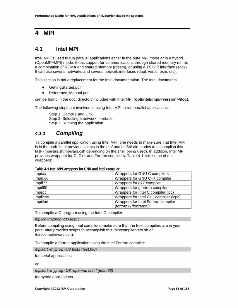
Performance Guide for HPC Applications on iDataPlex dx360 M4 systems
4 MPI
4.1 Intel MPI
Intel MPI is used to run parallel applications either in the pure MPI mode or in a hybrid (OpenMP+MPI) mode. It has support for communications through shared memory (shm), a combination of RDMA and shared memory (rdssm), or using a TCP/IP interface (sock). It can use several networks and several network interfaces (dapl, verbs, psm, etc).
This section is not a replacement for the Intel documentation. The Intel documents:
• GettingStarted.pdf • Reference_Manual.pdf
can be found in the doc/ directory included with Intel MPI (opt/intel/impi/<version>/doc).
The following steps are involved in using Intel MPI to run parallel applications:
Step 1: Compile and Link Step 2: Selecting a network interface Step 3: Running the application
4.1.1 Compiling
To compile a parallel application using Intel MPI, one needs to make sure that Intel MPI is in the path. Intel provides scripts in the bin/ and bin64/ directories to accomplish this task (mpivars.sh/mpivars.csh depending on the shell being used). In addition, Intel MPI provides wrappers for C, C++ and Fortran compilers. Table 4-1 lists some of the wrappers:
Table 4-1 Intel MPI wrappers for GNU and Intel compiler mpicc Wrappers for GNU C compilers mpicxx Wrappers for GNU C++ compiler mpif77 Wrappers for g77 compiler mpif90 Wrappers for gfortran compiler mpiicc Wrappers for Intel C compiler (icc) mpiicpc Wrappers for Intel C++ compiler (icpc) mpiifort Wrappers for Intel Fortran compiler
(fortran77/fortran95)
To compile a C-program using the Intel C-compiler: mpiicc -myprog -O3 test.c Before compiling using Intel compilers, make sure that the Intel compilers are in your path. Intel provides scripts to accomplish this (bin/compilervars.sh or /bin/compilervars.csh).
To compile a fortran application using the Intel Fortran compiler: mpiifort -myprog -O3 test.f (test.f90) for serial applications
or
mpiifort -myprog -O3 -openmp test.f (test.f90) for hybrid applications
Copyright ©2012 IBM Corporation
Page 61 of 153

Performance Guide for HPC Applications on iDataPlex dx360 M4 systems
4.1.2 Running Parallel Applications
Running parallel applications is a 2-step process: The first step is mpdboot This step will create supervisory processes called “mpds” on the nodes where the parallel application is run. The synatax is: mpdboot -n xx -f hostfile -r ssh where xx is the number of nodes (only one mpd instance runs on a node independent of the number of MPI tasks targeted for each node) and the hostfile contains the node names (one host per line).
To make sure that the mpdboot ran successfully, one can query the nodes in the parallel partition using mpdtrace which will list all of the nodes in the parallel partition. To force mpdboot to maintain the same order as in the hostfile, one can add an additional flag –ordered in the mpdboot command.
After mpdboot, one can run the parallel application using: mpiexec -perhost xx -np yy myprog or mpiexec -np yy -machinefile hf myprog
or mpiexec -np yy -machinefile hf ./myprog < stdin > stdout
where xx is the number of tasks on a node and yy is the total number of MPI tasks. The machinefile contains the list of the nodes where the MPI tasks will be run (one per line).
One can combine the functions of mpdboot and mpiexec by using mpirun instead.
After the parllel job has completed, issue mpdallexit
to close all of the python processes.
Intel MPI dynamically selects the appropriate fabric for communication among the MPI processes. To select a specific fabric for communication, set the environmental variable I_MPI_FABRICS. Table 4-2 provides some communication fabric settings.
Table 4-2 Intel MPI settings for I_MPI_FABRICS I_MPI_FABRICS Network fabric
shm:dapl Default setting
shm Shared-memory
dapl DAPL capable network fabrics eg. InfiniBand, iwarp etc..
tcp TCP/IP capable networks
tmi Tag Matching Interface (TMI) eg. Qlogic, Myrinet etc.
ofa InfiniBand over OFED verbs provided
Copyright ©2012 IBM Corporation
Page 62 of 153

Performance Guide for HPC Applications on iDataPlex dx360 M4 systems
I_MPI_FABRICS Network fabric
by Open Fabrics Alliance (OFA)
On a single node, use
I_MPI_FABRIC=shm
for communication through shared-memory. The I_MPI_FABRICS environmental variable can also be passed in the run command using mpiexec -genv I_MPI_FABRIC=ofa -np yy -machinefile hf ./myprog
4.1.3 Processor Binding
To find the way the binding is done on a node, one can use the cpuinfo command. The command output is: $ cpuinfo Intel(R) Xeon(R) CPU E5-2680 0 ===== Processor composition ===== Processors(CPUs) : 32 Packages(sockets) : 2 Cores per package : 8 Threads per core : 2 ===== Processor identification ===== Processor Thread Id. Core Id. Package Id. 0 0 0 0 1 0 1 0 2 0 2 0 3 0 3 0 4 0 4 0 5 0 5 0 6 0 6 0 7 0 7 0 8 0 0 1 9 0 1 1 10 0 2 1 11 0 3 1 12 0 4 1 13 0 5 1 14 0 6 1 15 0 7 1 16 1 0 0 17 1 1 0 18 1 2 0 19 1 3 0 20 1 4 0 21 1 5 0 22 1 6 0 23 1 7 0 24 1 0 1 25 1 1 1 26 1 2 1 27 1 3 1 28 1 4 1 29 1 5 1 30 1 6 1 31 1 7 1 ===== Placement on packages ===== Package Id. Core Id. Processors 0 0,1,2,3,4,5,6,7 (0,16)(1,17)(2,18)(3,19)(4,20)(5,21)(6,22)(7,23)
Copyright ©2012 IBM Corporation
Page 63 of 153
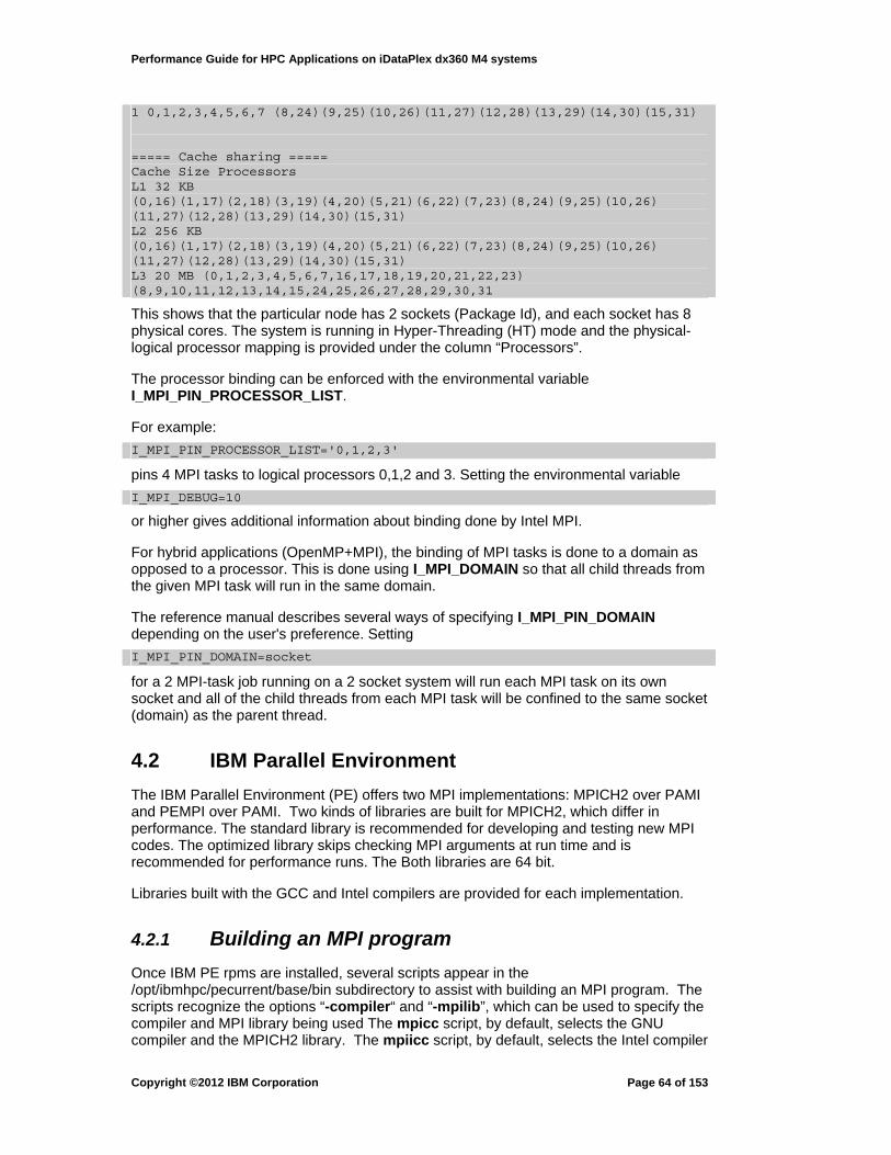
Performance Guide for HPC Applications on iDataPlex dx360 M4 systems
1 0,1,2,3,4,5,6,7 (8,24)(9,25)(10,26)(11,27)(12,28)(13,29)(14,30)(15,31) ===== Cache sharing ===== Cache Size Processors L1 32 KB (0,16)(1,17)(2,18)(3,19)(4,20)(5,21)(6,22)(7,23)(8,24)(9,25)(10,26) (11,27)(12,28)(13,29)(14,30)(15,31) L2 256 KB (0,16)(1,17)(2,18)(3,19)(4,20)(5,21)(6,22)(7,23)(8,24)(9,25)(10,26) (11,27)(12,28)(13,29)(14,30)(15,31) L3 20 MB (0,1,2,3,4,5,6,7,16,17,18,19,20,21,22,23) (8,9,10,11,12,13,14,15,24,25,26,27,28,29,30,31
This shows that the particular node has 2 sockets (Package Id), and each socket has 8 physical cores. The system is running in Hyper-Threading (HT) mode and the physical-logical processor mapping is provided under the column “Processors”.
The processor binding can be enforced with the environmental variable I_MPI_PIN_PROCESSOR_LIST.
For example: I_MPI_PIN_PROCESSOR_LIST='0,1,2,3'
pins 4 MPI tasks to logical processors 0,1,2 and 3. Setting the environmental variable
I_MPI_DEBUG=10
or higher gives additional information about binding done by Intel MPI.
For hybrid applications (OpenMP+MPI), the binding of MPI tasks is done to a domain as opposed to a processor. This is done using I_MPI_DOMAIN so that all child threads from the given MPI task will run in the same domain.
The reference manual describes several ways of specifying I_MPI_PIN_DOMAIN depending on the user's preference. Setting
I_MPI_PIN_DOMAIN=socket
for a 2 MPI-task job running on a 2 socket system will run each MPI task on its own socket and all of the child threads from each MPI task will be confined to the same socket (domain) as the parent thread.
4.2 IBM Parallel Environment
The IBM Parallel Environment (PE) offers two MPI implementations: MPICH2 over PAMI and PEMPI over PAMI. Two kinds of libraries are built for MPICH2, which differ in performance. The standard library is recommended for developing and testing new MPI codes. The optimized library skips checking MPI arguments at run time and is recommended for performance runs. The Both libraries are 64 bit.
Libraries built with the GCC and Intel compilers are provided for each implementation.
4.2.1 Building an MPI program
Once IBM PE rpms are installed, several scripts appear in the /opt/ibmhpc/pecurrent/base/bin subdirectory to assist with building an MPI program. The scripts recognize the options “-compiler“ and “-mpilib”, which can be used to specify the compiler and MPI library being used The mpicc script, by default, selects the GNU compiler and the MPICH2 library. The mpiicc script, by default, selects the Intel compiler
Copyright ©2012 IBM Corporation
Page 64 of 153

Performance Guide for HPC Applications on iDataPlex dx360 M4 systems
and the MPICH2 library. The PEMPI library is selected if the “-mpilib ibm_pempi” option is used.
4.2.2 Selecting MPICH2 libraries
The selection between standard and optimized libraries is done at run time. The standard library is chosen by default. If the MP_EUIDEVELOP=min environment variable setting is specified, the optimized MPICH2 library will be selected. A selection can be verified by checking library paths in the “/proc/<pid>/smaps” file for a process with process ID <pid>.
4.2.3 Optimizing for Short Messages
The best latency is achieved when the MPICH2 stack selects “lockless” mode where no locking takes place in MPI and PAMI. The MPICH2 library enters this mode if either MPI_Init() is called at initialization time or MPI_Init_thread() is called with an argument MPI_THREAD_SINGLE, which is the preferred way. Lockless mode is valid only when the main MPI thread makes MPI calls. Violations of this rule may cause data corruption.
To select lockless mode in a PEMPI program initialized by MPI_Init(), one has to set
export MP_SINGLE_THREAD=yes export MP_LOCKLESS=yes
in the environment. Note, these settings would not work with jobs which use one-sided MPI or MPI/IO functions.
MPICH2 implements a Reliable Connection (RC) FIFO mode on top of RC Transport to cut PAMI overhead associated with checking whether data sent unreliably actually arrived and with packet retransmission in cases when data is lost. This mode uses RC connections spanning a job’s lifetime between any pair of MPI tasks. The environment setting MP_RELIABLE_HW=yes will enable RC FIFO mode.
All of these optimizations are valid for any message size, but they have the greatest impact on short messages.
The best latency is achieved with the environment setting MP_INSTANCES=1 (default).
Short messages are defined as the lower bound for MP_BULK_MIN_MSG_SIZE (4K). The Maximum Transmission Unit (MTU) may impact latency. Setting MP_FIFO_MTU=2K is typically better for messages under 4KB.
4.2.4 Optimizing for Intranode Communications
Shared memory is the default for intranode communications. It usually gives the best performance but can be disabled by choosing MP_SHARED_MEMORY=no which will force messages to go over the IB fabric. In the context of collective operations in PEMPI, the explicit use of shared memory (as compared to the implicit use of shared memory via PAMI) does not always provide the best performance. The MP_SHMCC_EXCLUDE_LIST environment variable is provided for PEMPI to turn off explicit use of shared memory for a selected list of collective operations.
4.2.5 Optimizing for Large Messages
Large messages, by default, are transmitted via RDMA which uses RC connections. At
Copyright ©2012 IBM Corporation
Page 65 of 153

Performance Guide for HPC Applications on iDataPlex dx360 M4 systems
large scale, a job may run out of RC connections which consume memory proportionally to the number of RC connections. The default number of connections can be overridden by setting MP_RC_MAX_QP.
When the number of MPI tasks sharing a node is small, setting MP_INSTANCES to a value larger than one may help to improve bandwidth. Increasing the number of MP_INSTANCES will increase the number of RC connections accordingly.
By default, messages above 16KB are transmitted in RDMA mode (qualifying them as large messages). This is the crossover point between FIFO and RDMA modes. It can be overridden by setting MP_BULK_MIN_MSG_SIZE.
4.2.6 Optimizing for Intermediate-Size Messages
Short messages are transmitted via the Eager protocol where incoming messages are buffered on the receive side if no matching receive message is posted. This requires special buffers to be allocated on each node. Setting MP_EAGER_LIMIT will override the default message size at which the eager protocol is replaced by a Rendezvous protocol. MPI will honor the MP_EAGER_LIMIT value only if the early arrival buffer is big enough. The default buffer size can be overridden by setting MP_BUFFER_MEM .
On the send side, short messages are copied to a retransmission buffer. This allows MPI to return to user program while a message is in transit. The default buffer size can be overridden by setting MP_REXMIT_BUF_SIZE.
As implied by sections 4.2.3 and 4.2.5, intermediate-size messages are between 4KB and the RDMA crossover point (default 16KB, as set by MP_BULK_MIN_MSG_SIZE).
4.2.7 Optimizing for Memory Usage
For large task counts, a significant portion of memory can be consumed by RC RDMA connections. Should that become a scalability issue, a program may choose to run in FIFO mode.
This can be achieved by setting MP_USE_BULK_XFER=no. Buffer tuning environment variables MP_BUFFER_MEM and MP_RFIFO_SIZE can be set to reduce the MPI memory footprint.
For a small task count per node, FIFO mode is less efficient than RDMA.
A significant Improvement in network bandwidth can be achieved by setting MP_FIFO_MTU=4K. Note, a 4K MTU must be enabled on the switch for that to work.
4.2.8 Collective Offload in MPICH2
The ConnectX-2 adapter for QDR networks and the ConnectX-3 adapter for FDR10 and FDR networks, offer an interface called Fabric Collective Accelerator (FCA). FCA combines CORE-Direct® (Collective Offload Resource Engine) on the adapter with hardware assistance on the switch to speed up selected collective operations. Using FCA may significantly improve the performance of an application. Only MPICH2 supports collective offloading. The following MPI collectives are available with FCA:
• MPI_Reduce • MPI_Allreduce • MPI_Barrier
Copyright ©2012 IBM Corporation
Page 66 of 153
Performance Guide for HPC Applications on iDataPlex dx360 M4 systems
• MPI_Bcast • MPI_Allgather • MPI_Allgatherv
The list of supported data types includes:
• All data types for C language bindings, except MPI_LONG_DOUBLE • All data types for C reduction functions (C reduction types). • The following data types for FORTRAN language bindings: MPI_INTEGER,
MPI_INTEGER2, MPI_INTEGER4, MPI_INTEGER8, MPI_REAL, MPI_REAL4 and MPI_REAL8
• FCA does not support data types for FORTRAN reduction functions (FORTRAN reduction types).
By default, collective offload is turned off. To enable it, the environment variable MP_COLLECTIVE_OFFLOAD=[all | yes] must be set. Setting MP_COLLECTIVE_OFFLOAD=[none| no] disables collective offload. Once enabled, the FCA collective algorithm will be the first one MPICH2 will try. If the FCA algorithm cannot run at this time, a default MPICH2 algorithm will be executed. The FCA algorithm may not be available if a node has no FCA software installed, does not have a valid license, the FCA daemon is not running on the network, etc. FCA support is limited to 2K MPI communicators per network.
To enable a subset of supported FCA algorithms two environment variables MP_COLLECTIVE_OFFLOAD=[all | yes] and MP_MPI_PAMI_FOR=[<collective1>,…,<collectiveN>], where collectives in the list are identified as “Reduce”, “Allreduce”, “Barrier”, “Bcast”, “Allgather” and “AllGatherV”, must be set. All collectives outside the list will use default MPICH2 algorithm.
4.2.9 MPICH2 and PEMPI Environment Variables
MP_EUIDEVELOP=min
When set to “min”, selects the optimized MPICH2 library. The optimized library helps to reduce latency. The standard MPICH2 library is selected by default. (Note that the PEMPI library will skip some parameter checking when MP_EUIDEVELOP=min is used.)
MP_SINGLE_THREAD=[yes|no]
Avoids some PAMI locking overhead and improves short message latency when set to “yes”. MP_SINGLE_THREAD=yes is valid only for user programs which make MPI calls from a single thread. For mutithreaded processes with threads making concurrent MPI calls, setting MP_SINGLE_THREAD=yes, will cause inconsistent results. The default value is “no”.
MP_SHARED_MEMORY=[yes|no]
To specify the use of shared memory for intranode communications rather than network. The default value is “yes”. In a few cases disabling shared memory improves performance.
MP_SHMEM_PT2PT=[yes|no]
Specifies whether intranode point-to-point MPICH2 communication should use optimized, shared-memory protocols. Allowable values are “yes” and “no”. The default value is
Copyright ©2012 IBM Corporation
Page 67 of 153

Performance Guide for HPC Applications on iDataPlex dx360 M4 systems
“yes”.
MP_EAGER_LIMIT=<INTEGER>
Changes the message size threshold above which rendezvous protocol is used. This environment variable may be useful in reducing the latency for medium-size messages. Larger values increase the memory overhead.
MP_REXMIT_BUF_SIZE=<INTEGER>
Specifies the size of a local retransmission buffer (send side). The recommended value is the size of MP_EAGER_LIMIT plus 1K. It may help to reduce the latency of medium-size messages. Larger values increase memory overhead.
MP_FIFO_MTU=[2K|4K]
If a chassis MTU on the InfiniBand switch is 4K, the environment variable can be set to 4K. This will improve bandwidth for medium and large messages if a job is running in FIFO mode (MP_USE_BULK_XFER=no). It may have a negative impact on the latency of messages below 4K. The default value is 2K.
MP_RDMA_MTU=[2K|4K]
If a chassis MTU on the InfiniBand switch is 4K, the environment variable can be set to 4K. This may improve bandwidth for medium and large messages if a job is running in RDMA mode (MP_USE_BULK_XFER=yes). The default value is 2K.
MP_PULSE=<INTEGER>
The interval (in seconds) at which POE checks the remote nodes to ensure that they are communicating with the home node. Setting to “0” reduces jitter. The default value is “600”.
MP_INSTANCES=<INTEGER>
The number of instances corresponds to the number of IB Queue Pairs (QP) over which a single MPI task can stripe. Striping over multiple QPs improves network bandwidth in RDMA mode when a single instance does not saturate the link bandwidth. The default is one, which is usually sufficient when there are multiple MPI tasks per node.
MP_USE_BULK_XFER=[yes|no]
Enables bulk message transfer (RDMA mode). RDMA mode requires RC connections between each pair of communicating tasks which takes memory resources. The value “no” will turn on FIFO mode which is scalable. In some cases FIFO bandwidth outperforms RDMA bandwidth due to reduced contention in the switch. The default value is “yes”.
MP_BULK_MIN_MSG_SIZE=<INTEGER>
Sets the minimum message length for bulk transfer (RDMA mode). A valid range is from 4096 to 2147483647 (INT_MAX). Note, that for PEMPI, MP_EAGER_LIMIT value takes precedence if it is larger. MPICH2 ignores the value of MP_BULK_MIN_MSG_SIZE.
Copyright ©2012 IBM Corporation
Page 68 of 153
Performance Guide for HPC Applications on iDataPlex dx360 M4 systems
This environment variable can help optimize the crossover point between FIFO and RDMA modes.
MP_SHMCC_EXCLUDE_LIST= [ all | none | <list of collectives> ]
Use this environment variable to specify the collective communication routine in which the MPI level shared memory optimization should be disabled. The same can be done for a list of selected collective routines (separated by colons) : <list of collectives> = <collective1>:…:<collectiveN>.
The full list of collectives includes: "Barrier","Bcast","Reduce", "Allreduce","Reduce_scatter", "Gather", "Gatherv", "Scatter", "Scatterv", "Allgather", “Allgatherv", "Alltoall", "Alltoallv", "Alltoallw", "Scan", "Exscan”. The default is “none”. ”. It applies only to PEMPI.
MP_RC_MAX_QP=<INTEGER>
Specifies the maximum number of Reliable Connected Queue Pairs (RC QPs) that can be created. The purpose of MP_RC_MAX_QP is to limit the amount of memory that is consumed by RC QPs. This is recommended for applications which are close to or exceed the memory limit.
MP_RFIFO_SIZE=<INTEGER>
The default size of the receive FIFO used by each MPI task is 4MB. Larger jobs are recommended to use the maximum size receive FIFO (16MB) by setting MP_RFIFO_SIZE=16777216.
MP_BUFFER_MEM=<INTEGER>
Specifies the size of the Early Arrival buffer that is used by the communication subsystem to buffer eager messages arriving before a matching receive is posted. Setting MP_BUFFER_MEM can address “MPCI_MSG: ATTENTION: Due to memory limitation eager limit is reduced to X”. MP_BUFFER_MEM applies to PEMPI only.
MP_POLLING_INTERVAL=<INTEGER>
This defines the interval in microseconds at which the LAPI timer thread runs. Setting the polling interval equal to 800000 defines an 800 millisecond timer. The default is 400 milliseconds.
MP_RETRANSMIT_INTERVAL=<INTEGER>
PAMI will retransmit packets if an acknowledgement is not received in time. Retransmissions are costly and often unnecessary, generating duplicate packets. Setting a higher value will allow PAMI to tolerate larger delays before the retransmission logic kicks in.
4.2.10 IBM PE Standalone POE Affinity
When PE is used without a resource manager, POE provides standalone task affinity. This involves:
• For OpenMP jobs, MP_TASK_AFFINITY=cpu:n/core:n/primary:n options are
Copyright ©2012 IBM Corporation
Page 69 of 153
Performance Guide for HPC Applications on iDataPlex dx360 M4 systems
available for both Intel and GNU OpenMP implementations. Since PE does not know the OpenMP implementation in use (Intel or GNU), PE has to set the both GOMP_CPU_AFFINITY and KMP_AFFINITY for each task.
• For non-OpenMP jobs - using MP_TASK_AFFINITY=cpu, core, primary, or mcm - POE will examine the x86 device tree and determine the cpusets to which the tasks will be attached, using system level affinity API calls of sched_setaffinity.
Adapter affinity (MP_TASK_AFFINITY=sni) is not supported on x86 systems.
4.2.11 OpenMP Support
On the x86 Linux platform, PE provides affinity support for the Intel and GNU x86 platform OpenMP implementations, based on the KMP_AFFINITY and GOMP_CPU_AFFINITY variables. First POE will determine the number of parallel threads: for jobs involving a resource manager, POE expects the OMP_NUM_THREADS variable to be exported and set to the number of parallel threads.
When OMP_NUM_THREADS is not exported, POE will use the value of “n” in the MP_TASK_AFFINITY = core:n, cpu:n, or primary:n as the number of parallel threads.
For Intel, PE will set the KMP_AFFINITY variable, with a list of CPUs in the “proclist” sub-option value. Note POE has to allow for the user specified KMP_AFFINITY variable, and the list of CPUs to any existing options. If the user has already specified a “proclist” sub-option value, POE will override the user-specified value, while displaying an appropriate message. If MP_INFOLEVEL is set to 4 or higher, POE will also add the “verbose” option to KMP_AFFINITY. An example of the KMP_AFFINITY format POE will set (for MP_TASK_AFFINITY=cpu:4) is: KMP_AFFINITY=proclist=[3,2,1,0],explicit .
For GNU, PE will set the GOMP_CPU_AFFINITY variable correctly, to a comma-separated list of CPUs, one per thread, for each task. A sample format of the GOMP_CPU_AFFINITY (for MP_TASK_AFFINITY=cpu:4) is: GOMP_CPU_AFFINITY="0,2,4,6" .
Although GOMP_CPU_AFFINITY allows its values to be expressed as ranges or strides, POE will use a comma separated list of single CPU numbers, representing logical CPUs attached to the task. If the user has already specified a GOMP_CPU_AFFINITY value, POE will override the user-specified value, while displaying an appropriate message.
When MP_BINDPROC = yes is specified, POE will bind/attach the tasks based on the list of CPUs in the KMP_AFFINITY and GOMP_CPU_AFFINITY values.
4.3 Using LoadLeveler with IBM PE
4.3.1 Requesting Island Topology for a LoadLeveler Job
An island can be defined as a set of nodes connected to the same switch. Those switches can be interconnected via spine switches to form a larger network. Running a job within an island, typically, provides a better latency and bisection bandwidth than spreading it over multiple islands. Island topology can be requested by the node_topology keyword
# @ node_topology = none | island
A second JCF keyword, island_count
# @ island_count=minimun[,maximum]
Copyright ©2012 IBM Corporation
Page 70 of 153

Performance Guide for HPC Applications on iDataPlex dx360 M4 systems
specifies the minimum and maximum number of islands to select for this job step. A value of -1 represents all islands in the cluster.
If island_count is not specified, all machines will be selected from a common island.
The llstatus and llrstatus commands will be enhanced to show which island contains the machine or machine _group.
4.3.2 How to run OpenMPI and INTEL MPI jobs with LoadLeveler
To run OpenMPI jobs under LoadLeveler, a job command file, must specify a job type of ”MPICH”. A script that will launch a job built with OpenMPI version 1.5.4 is given below
# ! /bin/ksh # LoadLeveler JCF file for running an Open MPI job # @ job_type = MPICH # @ node = 4 # @ tasks_per_node = 2 # @ output = ompi_test.$(cluster).$(process).out # @ error = ompi_test.$(cluster).$(process).err # @ queue mpirun openmpi_test_program
For OpenMPI versions prior to 1.5.4, a user must specify the LoadLeveler run time environment variables LOADL_TOTAL_TASKS and LOADL_HOSTFILE, as arguments to the OpenMPI executable to indicate the number of tasks to start and where to start them. The user also specifies the LoadLeveler llspawn.stdio executable as the remote command for the OpenMPI executable to use when launching MPI tasks, and must specify the mpirun option, --leave-session-attached, which will keep the spawned MPI tasks descendents of LoadLeveler processes.
A script that will launch a job built with OpenMPI version older than 1.5.4 is given below
# ! /bin/ksh # LoadLeveler JCF file for running an Open MPI job # @ job_type = MPICH # @ node = 4 # @ tasks_per_node = 2 # @ output = ompi_test.$(cluster).$(process).out # @ error = ompi_test.$(cluster).$(process).err # @ queue export LD_LIBRARY_PATH=/opt/openmpi/lib /opt/openmpi/bin/mpirun -leave-session-attached --mca plm_rsh_agent "llspawn.stdio : ssh" -n $LOADL_HOSTFILE -machinefile $LOADL_HOSTFILE mpi_hello_sleep_openmpi
4.3.3 LoadLeveler JCF (Job Command File) Affinity Settings
LoadLeveler must be configured to enable affinity support, which includes the following steps
$ mkdir /dev/cpuset $ mount -t cpuset none /dev/cpuset
Copyright ©2012 IBM Corporation
Page 71 of 153

Performance Guide for HPC Applications on iDataPlex dx360 M4 systems
The LoadLeveler configuration file must contain keyword
RSET_SUPPORT = RSET_MCM_AFFINITY
The keyword SCHEDULE_BY_RESOURCES must have ConsumableCpus as one of the arguments. Without the above settings a job requesting affinity will not be dispatched by the central manager.
4.3.4 Affinity Support in LoadLeveler
The following JCF keywords support affinity in LoadLeveler on x86
1 # @ rset = RSET_MCM_AFFINITY 2 # @ mcm_affinity_options = mcm_mem_[req | pref] 3 # @ mcm_affinity_options =[mcm_distribute|mcm_accumulate] 4 # @ task_affinity = CORE(n) 5 # @ task_affinity = CPU(n) 6 # @ cpus_per_core = n 7 # @ parallel_threads = n
A job containing the mcm_affinity_options or task_affinity keywords will not be submitted to LoadLeveler unless the rset keyword is set to RSET_MCM_AFFINITY.
When mcm_mem_pref is specified, the job requests memory affinity as a preference. When mcm_mem_req is specified, the job requests memory affinity as a requirement. mcm_accumulate tells the central manager to accumulate tasks on the same MCM whenever possible.
mcm_distribute tells the central manager to distribute tasks across all available MCMs on a machine.
When CORE(n) or CPU(n) is specified, the central manager will assign n physical cores or n logical CPUs to each job task. (Note that a physical core can have multiple logical CPUs.)
cpus_per_core — specifies the number of logical CPUs per processor core that should be allocated to each task of a job with the processor-core affinity requirement (#@task_affinity = CORE). This requirement can be only satisfied by nodes configured in SMT mode.
parallel_threads=m — will bind m OpenMP threads to the CPUs selected for the task by task_affinity = CPU(n) keyword, where m <= n. If task_affinity = CORE(n) is specified, m OpenMP threads will be bound to m CPUs, one CPU per core.
The SMT setting can not be changed per job launch.
Copyright ©2012 IBM Corporation
Page 72 of 153

Performance Guide for HPC Applications on iDataPlex dx360 M4 systems
5 Performance Analysis Tools on Linux
5.1 Runtime Environment Control
5.1.1 Ulimit
The ulimit command controls user limits on jobs run interactively. Large HPC jobs often use more hardware resources than are given to users by default. These limits are put in place to make sure that program bugs and user errors don’t make the system unusable or crash. However, for benchmarking and workload characterization, it is best to set all resource limits to “unlimited” (or the highest allowed value) before running. This is especially true for resources like stack, memory and CPU time.
ulimit –s unlimited ulimit –m unlimited ulimit –t unlimited
5.1.2 Memory Pages The RHEL 6.2 and SLES 11.2 Linux distributions support a new kernel feature called transparent huge pages (THP). For HPC applications, using huge pages can reduce execution delays from missing in the TLB. As long as huge pages are available to the system, the user doesn’t need to do anything explicit to take advantage of them. The details are presented in section 3.2.
5.2 Hardware Performance Counters and Tools
The hardware in x86 processors provides performance counters for monitor events to understand performance and identify performance limiters. The Sandy Bridge processor provides 4 programmable counters and 3 fixed event counters. There are also uncore event counters that can be used to monitor L3, QPI and memory events. There are a number of tools that can be used to gather counter data. The use of perf for collecting counter data at the application level and the use of PAPI for instrumenting specific areas in the code will be covered here. perf ships with Linux but may need to be installed. (It may not be installed with the default set of packages). Other tools that can be used are vtune and likwid, but they will not be covered here. vtune requires a license from Intel to use. likwid can be found here; it does have some nice features.
For a description of the events available to count see chapter 19 in volume 3b of the Intel architecture manual.
For a guide on how to use these counters for analysis see appendix B.3 of the Intel Software Optimization guide. The general optimization material in the rest of the document is also recommended.
There is a good paper on bottleneck analysis using performance counters on the x86 5500 series processors, much of which is applicable to Sandy Bridge processors. It can be found here.
5.2.1 Hardware Event Counts using perf
perf is a suite of Linux tools that can be used for both collecting counter data and profiling. To check if perf is installed, enter the perf command. If it is available, the
Copyright ©2012 IBM Corporation
Page 73 of 153

Performance Guide for HPC Applications on iDataPlex dx360 M4 systems
command returns its help message; if not, it has to be installed. The installation varies by distribution, but to install on RHEL (as root) enter
$ yum install perf
Install on SLES (as root) with the command
$ zypper install perf
Also make sure if a new kernel is installed that perf gets updated the match the kernel
To use perf for collecting performance counters, the perf list and perf stat subcommands are used. See 'perf help' for more information on the subcommands available for perf. A tutorial is available here. For more information on any command enter ‘perf help COMMAND’.
Using the latest available version of perf is strongly recommended. Later versions provide more features.
The profiling aspect of perf will be covered in a later section. perf list is used to show the events available for the hardware being used. Any of the events can be appended with a colon followed by one or more modifiers that further qualify what will be counted. The modifiers are shown in the table below. Raw events can be modified with the same syntax as the symbolic events provided by perf list.
Table 5-1 Event modifiers for perf –e <event>:<mod> Modifier Action
u Count events in user mode k Count event in kernel mode h Count events in hypervisor mode
Default Count all events regardless of mode
perf list also shows software and tracepoint events, but the focus of this document is hardware counter events. These include the hardware, cache, and raw events. To see a list of the symbolic hardware events supported by perf for the current processor, use the command
$ perf list hardware
For the cache events supported, use the command
$ perf list cache
perf also supports raw event codes of the format rNNN where NNN represents the umask appended with the event decode. The format is described further by the command
$ perf list –help
5.2.1.1 Example 1
The first example demonstrates how to collect counts on built-in events with the command
$ perf stat
Events will be counted for the standard benchmark program stream. Download stream.c from here.
Modify the code to set the array size:
# define N 80000000
Copyright ©2012 IBM Corporation
Page 74 of 153
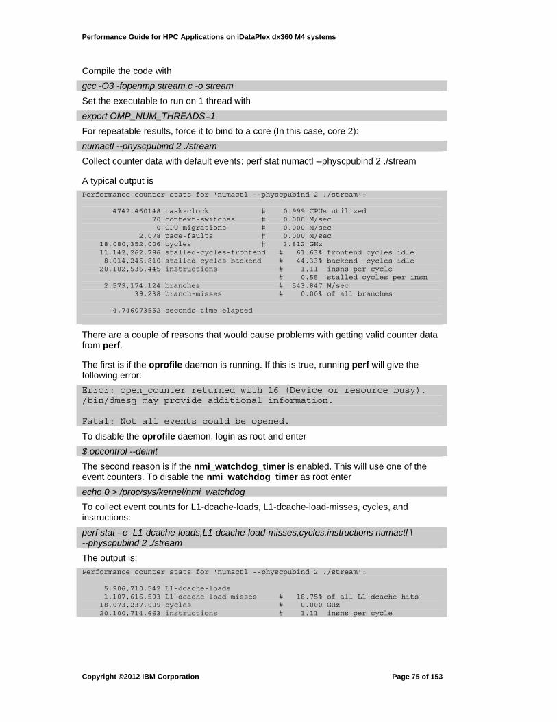
Performance Guide for HPC Applications on iDataPlex dx360 M4 systems
Compile the code with
gcc -O3 -fopenmp stream.c -o stream
Set the executable to run on 1 thread with
export OMP_NUM_THREADS=1
For repeatable results, force it to bind to a core (In this case, core 2):
numactl --physcpubind 2 ./stream
Collect counter data with default events: perf stat numactl --physcpubind 2 ./stream
A typical output is
Performance counter stats for 'numactl --physcpubind 2 ./stream': 4742.460148 task-clock # 0.999 CPUs utilized 70 context-switches # 0.000 M/sec 0 CPU-migrations # 0.000 M/sec 2,078 page-faults # 0.000 M/sec 18,080,352,006 cycles # 3.812 GHz 11,142,262,796 stalled-cycles-frontend # 61.63% frontend cycles idle 8,014,245,810 stalled-cycles-backend # 44.33% backend cycles idle 20,102,536,445 instructions # 1.11 insns per cycle # 0.55 stalled cycles per insn 2,579,174,124 branches # 543.847 M/sec 39,238 branch-misses # 0.00% of all branches 4.746073552 seconds time elapsed
There are a couple of reasons that would cause problems with getting valid counter data from perf.
The first is if the oprofile daemon is running. If this is true, running perf will give the following error:
Error: open_counter returned with 16 (Device or resource busy). /bin/dmesg may provide additional information. Fatal: Not all events could be opened.
To disable the oprofile daemon, login as root and enter
$ opcontrol --deinit
The second reason is if the nmi_watchdog_timer is enabled. This will use one of the event counters. To disable the nmi_watchdog_timer as root enter
echo 0 > /proc/sys/kernel/nmi_watchdog
To collect event counts for L1-dcache-loads, L1-dcache-load-misses, cycles, and instructions:
perf stat –e L1-dcache-loads,L1-dcache-load-misses,cycles,instructions numactl \ --physcpubind 2 ./stream
The output is:
Performance counter stats for 'numactl --physcpubind 2 ./stream': 5,906,710,542 L1-dcache-loads 1,107,616,593 L1-dcache-load-misses # 18.75% of all L1-dcache hits 18,073,237,009 cycles # 0.000 GHz 20,100,714,663 instructions # 1.11 insns per cycle
Copyright ©2012 IBM Corporation
Page 75 of 153

Performance Guide for HPC Applications on iDataPlex dx360 M4 systems
5.2.1.2 Example 2
The next example includes the syntax for a raw event. UOPS_ISSUED.ANY is collected in addition to the counters above. Section 19.3 of the architecture manual 3b provides the umask “01” and the event number “0x0e”. The raw code concatenates the two - “010e”. An alternative way to get the mask and event code is to use libpfm4. Install libpfm4 and go into the examples directory. The utility showevtinfo will give the event codes and umasks for the current processor.
Enter the command:
perf stat -e r10e,L1-dcache-loads,L1-dcache-load-misses,cycles,instructions numactl \ --physcpubind 2 ./stream
This should produce something like:
Performance counter stats for 'numactl --physcpubind 2 ./stream': 24,228,890,952 r10e 5,906,666,765 L1-dcache-loads 1,107,547,809 L1-dcache-load-misses # 18.75% of all L1-dcache hits 18,063,959,547 cycles # 0.000 GHz 20,100,581,873 instructions # 1.11 insns per cycle 4.742253967 seconds time elapsed
Notice the output gives the raw code instead of the event name. Using libpfm4 and a couple of scripts provides the translation from a raw code to a symbolic name. The two scripts are
Code Listing 1 get_event_dict.awk # get_event_dict.awk BEGIN { mfound = 1; printf ("event_names = {\n"); } { if ( $1 == "PMU") { if (mfound == 0) { if ((type == "wsm_dp") || (type == "ix86arch")) printf(" \'0x%s\':\'%s\',\n", code1, name); } mfound = 0; type = $4 } if ( $1 == "Name") { name = $3; } if ( $1 == "Code") { code1 = substr($3,3); if (length(code) == 1) { code = "0" code1 } } if ( substr($1,1,5) == "Umask" ) { mfound = 1; mask=substr($3,3); if(index(mask,"0") == 1) mask = substr(mask,2)
Copyright ©2012 IBM Corporation
Page 76 of 153
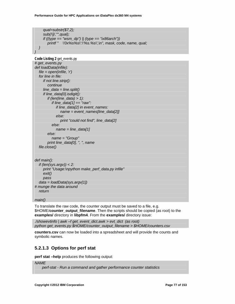
Performance Guide for HPC Applications on iDataPlex dx360 M4 systems
qual=substr($7,2); sub(/\]/,"",qual); if ((type == "wsm_dp") || (type == "ix86arch")) printf " \'0x%s%s\':\'%s.%s\',\n", mask, code, name, qual; } }
Code Listing 2 get_events.py # get_events.py def loadData(infile): file = open(infile, 'r') for line in file: if not line.strip(): continue line_data = line.split() if line_data[0].isdigit(): if (len(line_data) > 1): if line_data[1] == "raw": if line_data[2] in event_names: name = event_names[line_data[2]] else: print "could not find", line_data[2] else: name = line_data[1] else: name = "Group" print line_data[0], ", ", name file.close() def main(): if (len(sys.argv)) < 2: print "Usage:\npython make_perf_data.py infile" exit() pass data = loadData(sys.argv[1]) # munge the data around return main()
To translate the raw code, the counter output must be saved to a file, e.g. $HOME/counter_output_filename. Then the scripts should be copied (as root) to the examples/ directory in libpfm4. From the examples/ directory issue:
./showevtinfo | awk –f get_event_dict.awk > evt_dict (as root) python get_events.py $HOME/counter_output_filename > $HOME/counters.csv
counters.csv can now be loaded into a spreadsheet and will provide the counts and symbolic names.
5.2.1.3 Options for perf stat
perf stat –help produces the following output:
NAME perf-stat - Run a command and gather performance counter statistics
Copyright ©2012 IBM Corporation
Page 77 of 153
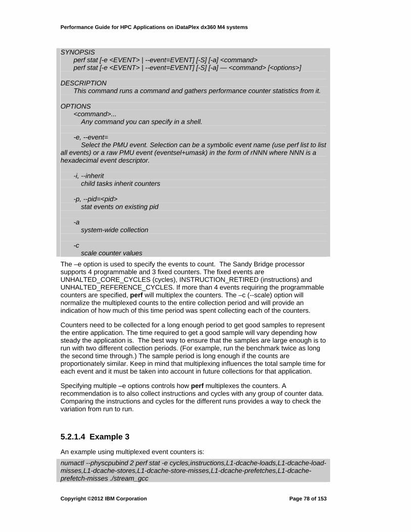
Performance Guide for HPC Applications on iDataPlex dx360 M4 systems
SYNOPSIS perf stat [-e <EVENT> | --event=EVENT] [-S] [-a] <command> perf stat [-e <EVENT> | --event=EVENT] [-S] [-a] — <command> [<options>] DESCRIPTION This command runs a command and gathers performance counter statistics from it. OPTIONS <command>... Any command you can specify in a shell. -e, --event= Select the PMU event. Selection can be a symbolic event name (use perf list to list all events) or a raw PMU event (eventsel+umask) in the form of rNNN where NNN is a hexadecimal event descriptor. -i, --inherit child tasks inherit counters -p, --pid=<pid> stat events on existing pid -a system-wide collection -c scale counter values
The –e option is used to specify the events to count. The Sandy Bridge processor supports 4 programmable and 3 fixed counters. The fixed events are UNHALTED_CORE_CYCLES (cycles), INSTRUCTION_RETIRED (instructions) and UNHALTED_REFERENCE_CYCLES. If more than 4 events requiring the programmable counters are specified, perf will multiplex the counters. The –c (--scale) option will normalize the multiplexed counts to the entire collection period and will provide an indication of how much of this time period was spent collecting each of the counters.
Counters need to be collected for a long enough period to get good samples to represent the entire application. The time required to get a good sample will vary depending how steady the application is. The best way to ensure that the samples are large enough is to run with two different collection periods. (For example, run the benchmark twice as long the second time through.) The sample period is long enough if the counts are proportionately similar. Keep in mind that multiplexing influences the total sample time for each event and it must be taken into account in future collections for that application.
Specifying multiple –e options controls how perf multiplexes the counters. A recommendation is to also collect instructions and cycles with any group of counter data. Comparing the instructions and cycles for the different runs provides a way to check the variation from run to run.
5.2.1.4 Example 3
An example using multiplexed event counters is:
numactl --physcpubind 2 perf stat -e cycles,instructions,L1-dcache-loads,L1-dcache-load-misses,L1-dcache-stores,L1-dcache-store-misses,L1-dcache-prefetches,L1-dcache-prefetch-misses ./stream_gcc
Copyright ©2012 IBM Corporation
Page 78 of 153

Performance Guide for HPC Applications on iDataPlex dx360 M4 systems
The output is: Performance counter stats for './stream_gcc': 17,917,691,998 cycles # 0.000 GHz [57.14%] 17,138,124,280 instructions # 0.96 insns per cycle [71.43%] 5,106,659,829 L1-dcache-loads [71.43%] 1,108,292,001 L1-dcache-load-misses # 21.70% of all L1-dcache hits [71.43%] 1,901,538,315 L1-dcache-stores [71.43%] 473,207,328 L1-dcache-store-misses [71.45%] 821,116,783 L1-dcache-prefetch-misses [57.16%] 4.739070694 seconds time elapsed
The output reports a total runtime of 4.74 seconds. The percentage in the square brackets shows what percentage of 4.74 seconds was used while collecting for that particular counter. The perf output automatically adjusts for multiplexing so that the count displayed represents the actual count divided by the percentage collected.
To collect events for a job that is already running (under numactl binding control) or for a certain process of a job, perf can be used with the –p and –a options while running the sleep command. If the job is multitasked or multithreaded, using the –i flag collects event counts for all child processes.
perf –p <pid> -a –i sleep <data collection interval>
Attaching to an already running job is the technique to use if
• the job runs for a long time and event data can be collected for a shorter time (the length of the “sleep)
• the job has a “warm up” period that needs to be excluded from the event counts. • a specific job phase has to be reached before collecting event counts.
These are the basics of collecting counter data. The question now becomes which events should be collected for analysis? Start out with the basic events needed for CPI, instruction mix, cache miss rates, ROB and RAT stalls, and branch prediction metrics. For programs that use large arrays, data on L1TLB and L2TLB misses is also useful. Some other things to consider are the use of vector instructions and the effectiveness of prefetching. What is needed will depend on what performance issues need to be understood.
5.2.2 Instrumenting Hardware Performance with PAPI
perf is good for collecting performance data on an entire application. perf also has an API for collecting counter data, but the perf interface is not documented.
To collect data on a specific portion of a program, the PAPI (Performance Application Programming Interface) library is recommended for instrumenting the source code. The PAPI source tarball, installation instructions and other documentation are available from here. Some of the Linux distributions include a prepackaged version of PAPI, but downloading and installing PAPI is recommended. PAPI supports collecting performance event counts on a variety of systems including x86 Linux, Power Linux, and Power AIX.
A high level overview of PAPI is here. The examples/ and ctests/ subdirectories in the PAPI tree have additional useful information. The instrumentation examples in this document use the low-level API which is documented here. There is no support for this library, so, as mentioned in the previous section, if there are problems collecting performance data, look first at conflicts with oprofile or the nmi_watchdog_timer.
The functionality needed to use PAPI to collect counter data is:
1) select the events to collect 2) initialize PAPI
Copyright ©2012 IBM Corporation
Page 79 of 153
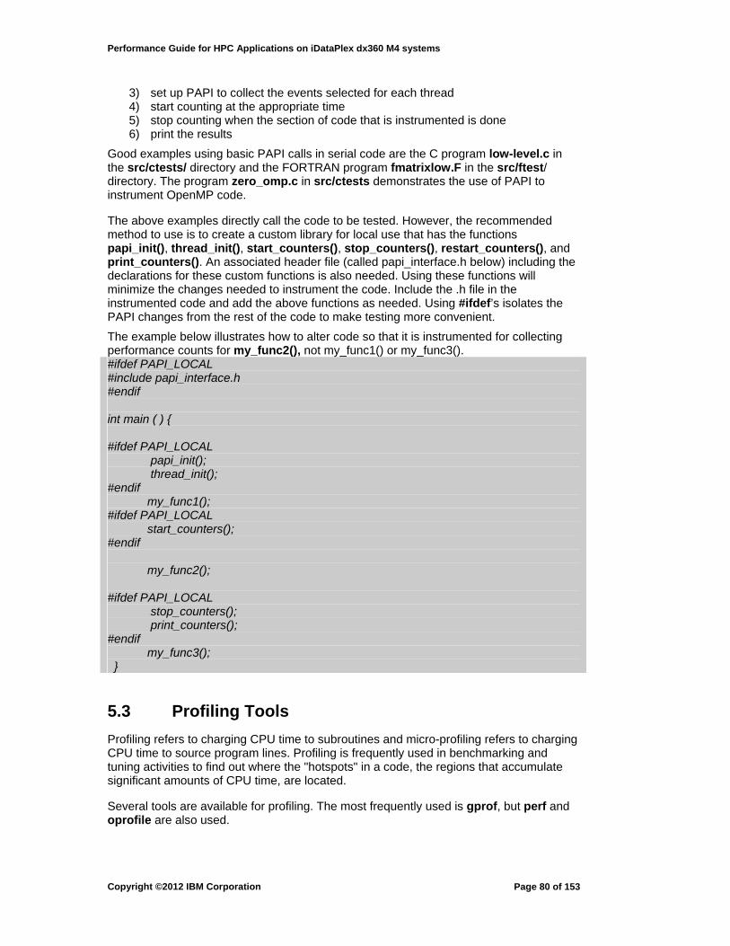
Performance Guide for HPC Applications on iDataPlex dx360 M4 systems
3) set up PAPI to collect the events selected for each thread 4) start counting at the appropriate time 5) stop counting when the section of code that is instrumented is done 6) print the results
Good examples using basic PAPI calls in serial code are the C program low-level.c in the src/ctests/ directory and the FORTRAN program fmatrixlow.F in the src/ftest/ directory. The program zero_omp.c in src/ctests demonstrates the use of PAPI to instrument OpenMP code.
The above examples directly call the code to be tested. However, the recommended method to use is to create a custom library for local use that has the functions papi_init(), thread_init(), start_counters(), stop_counters(), restart_counters(), and print_counters(). An associated header file (called papi_interface.h below) including the declarations for these custom functions is also needed. Using these functions will minimize the changes needed to instrument the code. Include the .h file in the instrumented code and add the above functions as needed. Using #ifdef’s isolates the PAPI changes from the rest of the code to make testing more convenient.
The example below illustrates how to alter code so that it is instrumented for collecting performance counts for my_func2(), not my_func1() or my_func3(). #ifdef PAPI_LOCAL #include papi_interface.h #endif int main ( ) { #ifdef PAPI_LOCAL papi_init(); thread_init(); #endif my_func1(); #ifdef PAPI_LOCAL start_counters(); #endif my_func2(); #ifdef PAPI_LOCAL stop_counters(); print_counters(); #endif my_func3(); }
5.3 Profiling Tools
Profiling refers to charging CPU time to subroutines and micro-profiling refers to charging CPU time to source program lines. Profiling is frequently used in benchmarking and tuning activities to find out where the "hotspots" in a code, the regions that accumulate significant amounts of CPU time, are located.
Several tools are available for profiling. The most frequently used is gprof, but perf and oprofile are also used.
Copyright ©2012 IBM Corporation
Page 80 of 153
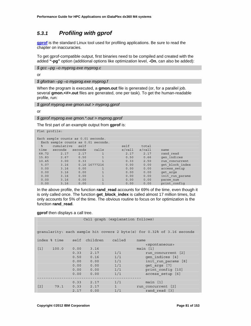
Performance Guide for HPC Applications on iDataPlex dx360 M4 systems
5.3.1 Profiling with gprof
gprof is the standard Linux tool used for profiling applications. Be sure to read the chapter on inaccuracies.
To get gprof-compatible output, first binaries need to be compiled and created with the added “-pg” option (additional options like optimization level, -On, can also be added):
$ gcc –pg –o myprog.exe myprog.c
or
$ gfortran –pg –o myprog.exe myprog.f
When the program is executed, a gmon.out file is generated (or, for a parallel job. several gmon.<#>.out files are generated, one per task). To get the human-readable profile, run:
$ gprof myprog.exe gmon.out > myprog.gprof
or
$ gprof myprog.exe gmon.*.out > myprog.gprof
The first part of an example output from gprof is:
Flat profile: Each sample counts as 0.01 seconds. Each sample counts as 0.01 seconds. % cumulative self self total time seconds seconds calls s/call s/call name 68.72 2.17 2.17 1 2.17 2.17 rand_read 15.83 2.67 0.50 1 0.50 0.66 gen_indices 10.45 3.00 0.33 1 0.33 2.50 run_concurrent 5.07 3.16 0.16 16777216 0.00 0.00 get_block_index 0.00 3.16 0.00 1 0.00 0.00 access_setup 0.00 3.16 0.00 1 0.00 0.00 get_args 0.00 3.16 0.00 1 0.00 0.00 init_run_params 0.00 3.16 0.00 1 0.00 0.00 parse_num 0.00 3.16 0.00 1 0.00 0.00 print_config
In the above profile, the function rand_read accounts for 69% of the time, even though it is only called once. The function get_block_index is called almost 17 million times, but only accounts for 5% of the time. The obvious routine to focus on for optimization is the function rand_read.
gprof then displays a call tree.
Call graph (explanation follows) granularity: each sample hit covers 2 byte(s) for 0.32% of 3.16 seconds index % time self children called name <spontaneous> [1] 100.0 0.00 3.16 main [1] 0.33 2.17 1/1 run_concurrent [2] 0.50 0.16 1/1 gen_indices [4] 0.00 0.00 1/1 init_run_params [8] 0.00 0.00 1/1 get_args [7] 0.00 0.00 1/1 print_config [10] 0.00 0.00 1/1 access_setup [6] ----------------------------------------------- 0.33 2.17 1/1 main [1] [2] 79.1 0.33 2.17 1 run_concurrent [2] 2.17 0.00 1/1 rand_read [3]
Copyright ©2012 IBM Corporation
Page 81 of 153

Performance Guide for HPC Applications on iDataPlex dx360 M4 systems
----------------------------------------------- 2.17 0.00 1/1 run_concurrent [2] [3] 68.7 2.17 0.00 1 rand_read [3] ----------------------------------------------- 0.50 0.16 1/1 main [1] [4] 20.9 0.50 0.16 1 gen_indices [4] 0.16 0.00 16777216/16777216 get_block_index [5] ----------------------------------------------- 0.16 0.00 16777216/16777216 gen_indices [4] [5] 5.1 0.16 0.00 16777216 get_block_index [5] ----------------------------------------------- 0.00 0.00 1/1 main [1] [6] 0.0 0.00 0.00 1 access_setup [6] ----------------------------------------------- 0.00 0.00 1/1 main [1] [7] 0.0 0.00 0.00 1 get_args [7] 0.00 0.00 1/1 parse_num [9] ----------------------------------------------- 0.00 0.00 1/1 main [1] [8] 0.0 0.00 0.00 1 init_run_params [8] ----------------------------------------------- 0.00 0.00 1/1 get_args [7] [9] 0.0 0.00 0.00 1 parse_num [9] ----------------------------------------------- 0.00 0.00 1/1 main [1] [10] 0.0 0.00 0.00 1 print_config [10] -----------------------------------------------
The call tree shows the caller for each of the functions.
gprof can also be used to tell the number of times a line of code is executed. This is done using the gcov tool. See the documentation here for more details.
5.3.2 Microprofiling
Microprofiling is defined as charging counter events to instructions (in contrast to event counts for an entire program as discussed in Section 5.2.1, or by function as discussed in Section 5.3.1). This is typically done with a sampling-based profile. Sampling-based profiling uses the overflow bit out of a counter to generate an interrupt and capture an instruction address. The profiling tool can be set up to interrupt after a specified number of cycles. Based on the number of times an instruction address shows up versus the total number of samples, the instruction is assigned that percentage of the total number of event occurrences.
There are three main tools used for microprofiling: vtune, perf and oprofile. All can use cycles (time) or another counter event to do profiling. Only perf and oprofile will be covered in this document since vtune requires a license to run.
5.3.2.1 Microprofiling with perf
perf uses cycles as its trigger event by default. This provides a list of instructions where the program is spending time. To sample the program with the cycles event, enter
perf record [prog_name] [prog_args] perf outputs some statistics and a file called perf.data. One key point is that the perf command has to be bound to a CPU to get reproducible results.
Copyright ©2012 IBM Corporation
Page 82 of 153

Performance Guide for HPC Applications on iDataPlex dx360 M4 systems
An example output from perf using binding is: # Events: 3K cycles # # Overhead Command Shared Object Symbol # ........ ....... ................. .......................... # 66.03% rand_rd rand_rd [.] rand_read 14.81% rand_rd rand_rd [.] gen_indices 5.37% rand_rd rand_rd [.] run_concurrent 4.47% rand_rd rand_rd [.] get_block_index 3.79% rand_rd [kernel.kallsyms] [k] clear_page_c 1.83% rand_rd libc-2.14.so [.] __random_r 1.34% rand_rd libc-2.14.so [.] __random 0.70% rand_rd libc-2.14.so [.] rand 0.27% rand_rd rand_rd [.] rand@plt 0.15% rand_rd [kernel.kallsyms] [k] get_page_from_freelist 0.12% rand_rd [kernel.kallsyms] [k] __kunmap_atomic 0.09% rand_rd [kernel.kallsyms] [k] run_posix_cpu_timers 0.09% rand_rd [kernel.kallsyms] [k] __kmap_atomic 0.06% rand_rd [kernel.kallsyms] [k] free_pages_prepare 0.06% rand_rd [kernel.kallsyms] [k] run_timer_softirq 0.06% rand_rd [kernel.kallsyms] [k] smp_apic_timer_interrupt 0.06% rand_rd [kernel.kallsyms] [k] update_cpu_load 0.06% rand_rd [kernel.kallsyms] [k] __might_sleep 0.03% rand_rd [kernel.kallsyms] [k] native_write_msr_safe
Notice this output includes system call and kernel functions.
perf annotate can be used to see where the program is spending its time. To get more detail on the rand_read function, enter
perf annotate rand_read
The output is:
: /* j gets set to a random index in rarray */ : j = indices[i]; 0.05 : 401209: 8b 45 f8 mov -0x8(%rbp),%eax 0.00 : 40120c: 48 98 cltq 0.00 : 40120e: 48 c1 e0 02 shl $0x2,%rax 1.75 : 401212: 48 03 45 e0 add -0x20(%rbp),%rax 0.00 : 401216: 8b 00 mov (%rax),%eax 0.09 : 401218: 89 45 f0 mov %eax,-0x10(%rbp) : k += rarray[j]; 0.05 : 40121b: 8b 45 f0 mov -0x10(%rbp),%eax 1.85 : 40121e: 48 98 cltq 0.00 : 401220: 48 c1 e0 03 shl $0x3,%rax 0.00 : 401224: 48 03 45 e8 add -0x18(%rbp),%rax 0.00 : 401228: 48 8b 00 mov (%rax),%rax 87.86 : 40122b: 89 c2 mov %eax,%edx 2.03 : 40122d: 8b 45 f4 mov -0xc(%rbp),%eax 0.09 : 401230: 01 d0 add %edx,%eax 1.57 : 401232: 89 45 f4 mov %eax,-0xc(%rbp)
The line
k += rarray[j];
is taking most of the time, with the assembly instruction
40122b: 89 c2 mov %eax,%edx
getting assigned 88% of the total time.
The –e option on perf record allows other events besides cycles to be used. This is useful to figure out which specific lines of code are strongly associated with events like
Copyright ©2012 IBM Corporation
Page 83 of 153
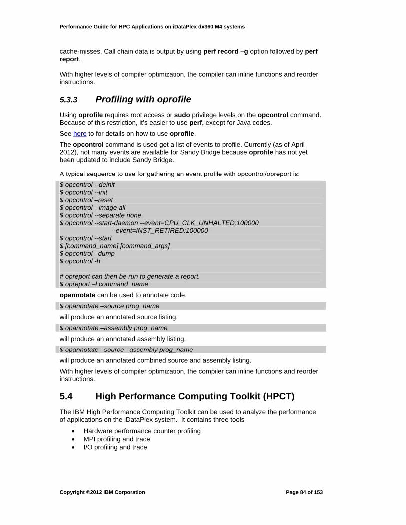
Performance Guide for HPC Applications on iDataPlex dx360 M4 systems
cache-misses. Call chain data is output by using perf record –g option followed by perf report.
With higher levels of compiler optimization, the compiler can inline functions and reorder instructions.
5.3.3 Profiling with oprofile
Using oprofile requires root access or sudo privilege levels on the opcontrol command. Because of this restriction, it’s easier to use perf, except for Java codes.
See here to for details on how to use oprofile.
The opcontrol command is used get a list of events to profile. Currently (as of April 2012), not many events are available for Sandy Bridge because oprofile has not yet been updated to include Sandy Bridge.
A typical sequence to use for gathering an event profile with opcontrol/opreport is:
$ opcontrol --deinit $ opcontrol --init $ opcontrol –reset $ opcontrol --image all $ opcontrol --separate none $ opcontrol --start-daemon --event=CPU_CLK_UNHALTED:100000 --event=INST_RETIRED:100000 $ opcontrol --start $ [command_name] [command_args] $ opcontrol –dump $ opcontrol -h # opreport can then be run to generate a report. $ opreport –l command_name
opannotate can be used to annotate code.
$ opannotate –source prog_name
will produce an annotated source listing.
$ opannotate –assembly prog_name
will produce an annotated assembly listing.
$ opannotate –source –assembly prog_name
will produce an annotated combined source and assembly listing.
With higher levels of compiler optimization, the compiler can inline functions and reorder instructions.
5.4 High Performance Computing Toolkit (HPCT)
The IBM High Performance Computing Toolkit can be used to analyze the performance of applications on the iDataPlex system. It contains three tools
• Hardware performance counter profiling • MPI profiling and trace • I/O profiling and trace
Copyright ©2012 IBM Corporation
Page 84 of 153

Performance Guide for HPC Applications on iDataPlex dx360 M4 systems
5.4.1 Hardware Performance Counter Collection
The hardware performance counter tool reads the hardware performance counters built into the system CPUs and accumulates performance measurements based on those counters. There are three ways to obtain hardware performance counter-based measurements
• System level reporting where system-wide hardware performance counters are queried and reported on a periodic basis
• Overall hardware performance counter values for the entire application • Hardware performance counter values for specific blocks of code, obtained by
editing the application source, adding calls to obtain hardware performance counter values and then recompiling and re-linking the application.
The hardware performance counter tool supports Nehalem1, Westmere2, and Sandy Bridge3 x86-based processors.
The hpcstat command collects hardware performance counter measurements on a system-wide basis. For instance, to query hardware performance counter group 2 every 5 seconds for 10 iterations, issue the command
$ hpcstat –g 2 –C 10 -I 5
The hpccount command collects hardware performance counter measurements over an entire run of an application. For instance, to get a total event count for hardware performance counter group 2 for the program shallow, issue the command
$ hpccount –g 2 shallow
To get hardware performance counter measurements for specific regions of code inside an application, the application source must be modified to call the hpmStart and hpmStop functions at appropriate points. Then the application should be recompiled with the –g flag and linked with the libhpc library.
For instance, when compiling the program petest, the commands to use are
$ gcc -c -g –I/opt/ibmhpc/ppedev.hpct/include petest.c $ gcc –o petest –g –L/opt/ibmhpc/ppedev.hpct/lib64 -lhpc
Before running the application, the HPM_EVENT_SET environment variable has to be set to the correct hardware counter group. The hpccount –l command lists available groups.
5.4.2 MPI Profiling and Tracing
The MPI profiling and trace tool provides summary performance information for each MPI function call in an application. This summary contains a count of how many times an MPI function call was executed, the time consumed by that MPI function call and, for communications calls, the total number of bytes transferred by that function call.
It also provides a time-based trace view which shows a trace of MPI function calls in the application. This trace can be used to examine MPI communication patterns. Individual trace events provide information about the time spent in that MPI function call and, for communication calls, the number of bytes transferred for that trace event.
1 The product list of Nehalem processors is found here (EP and EX) .
2 The product list of Westmere processors is found here (EP and EX).
3 The product list of Sandy Brtidge processors is found here and here,
Copyright ©2012 IBM Corporation
Page 85 of 153
Performance Guide for HPC Applications on iDataPlex dx360 M4 systems
To use the MPI profiling and trace tool, the application must be relinked with the profiling and trace library. A programming API is provided so that an application can be instrumented to selectively trace a subset of MPI function calls.
When compiling an application, it should be compiled with the –g flag. When linking the application, link with the libmpitrace library.
For instance, to compile when compiling the program petest, the commands to use are
$ gcc -c petest.c $ gcc –o petest –g –L/opt/ibmhpc/ppedev.hpct/lib64 -lmpitrace
5.4.3 I/O Profiling and Tracing
The I/O profiling and trace tool provides summary information about each system I/O call in your application. This information includes the number of times the I/O call was issued, the total time consumed by that function call, and for reads and writes, the number of bytes transferred by that system call.
It also provides a time-based trace view which shows more detailed information about the I/O system calls.
To use the I/O profiling and trace tool, you must re-link your application with the profiling and trace library.
When you compile your application, it should be compiled with the –g flag. When you link your application, you must link with the libtkio library.
For instance, to compile the program petest, use the commands
$ gcc -c petest.c $ gcc –o petest –g –L/opt/ibmhpc/ppedev.hpct/lib64 -ltkio
5.4.4 Other Information
The HPC Toolkit provides an X11-based viewer which can be used to examine performance data generated by these tools.
Current documentation for the HPC Toolkit can be found on the HPC Central website. The documentation web page is here. Click the Attachments tab and download the latest version of the documentation.
The HPC Toolkit is part of the IBM Parallel Environment (PE) Developer Edition product. PE Developer Edition is an Eclipse-based IDE that you can use to edit, compile, debug and run your application. PE Developer Edition also contains a plug-in for HPC Toolkit that is integrated with the rest of the developer environment and provides the same viewing capabilities as the X11-based viewer that is part of HPC Toolkit. Since the plug-in for HPC Toolkit is integrated with Eclipse, an instrumented application can be run from within the Eclipse IDE to obtain performance measurements.
Current documentation for the IDE contained in PE Developer Edition can be found here.
The HPC Toolkit is installed if the ppedev runtime RPM is present (rpm –qi ppedev_runtime) on all of the nodes in the cluster and that the ppedev_hpct RPM is installed on the login nodes in the cluster.
When using the HPC Toolkit to analyze the performance of parallel applications, the IBM
Copyright ©2012 IBM Corporation
Page 86 of 153

Performance Guide for HPC Applications on iDataPlex dx360 M4 systems
Parallel Environment Runtime Edition product must be installed on all of the nodes of the cluster.
PE Developer Edition, including HPC Toolkit, is supported on Red Hat 6 and SLES 11 SP1 x86 based Linux systems.
The Eclipse IDE environment provided by PE Developer Edition requires that either Eclipse 3.7 SR2 (Indigo) is already installed or that the version of Eclipse 3.7 SR2 packaged with PE Developer Edition is installed. Also, for Windows- and Linux-based systems, the IBM Java version 6 packaged with PE Developer Edition must be installed. For Mac users, the version of Java provided by default is all that is required.
Copyright ©2012 IBM Corporation
Page 87 of 153

Performance Guide for HPC Applications on iDataPlex dx360 M4 systems
6 Performance Results for HPC Benchmarks
6.1 Linpack (HPL)
6.1.1 Hardware and Software Stack Used The base system for section 6.1.3 used nodes featuring Intel Xeon E5-2670 ("Sandy Bridge-EP") 2.60 GHz, 64 Go (8x8 Go) DDR3 1333 MHz, and InfiniBand FDR Mellanox.
The software stack featured RedHat Enterprise Linux Server 6.1 64-bit, Intel Compilers 12.1, Intel MPI 4.0.3 and Intel MKL 10.3.7.256.
6.1.2 Code Version
Rather than using the original HPL source code (available for download from the Netlib Repository. It is strongly suggested to opt for the Intel Optimized MP LINPACK Benchmark for Clusters, which is provided for free as part of the Intel MKL library. This LINPACK version is fully compliant with TOP500 submissions.
This version brings several improvements to the original version, including in particular:
• The possibility to run the benchmark in hybrid mode (MPI + OpenMP). • The "As You Go" feature which reports information on achieved performance
level throughout the whole run. The feature evaluates the intrinsic quality of an execution configuration without the need to wait for the end of the execution.
6.1.3 Test Case Configuration
In order to reach the optimal level of performance, it is crucial to select a proper LINPACK configuration.
The main execution parameters are the following:
1. Matrix Size (N) The matrix size constitutes the size of the problem to be solved (number of elements). It has a direct impact on the memory usage on the computation nodes. Each matrix element is a variable of type double.
2. Block Size (NB) 3. Grid Size & Shape (PxQ)
The following criteria must be taken into account when defining a LINPACK configuration:
Table 6-1 LINPACK Job Parameters Parameters Constraints
N
Matrix size must be sized to fit the available memory on computation nodes: (N^2 * 8) / NB Nodes < Available Memory Per Node Note: available memory per node must take Operating System consumption into account
N / NB Number of blocks per dimension must be an integer: N modulo NB = 0
P x Q Number of grid elements must be equal to the number of MPI processes
Copyright ©2012 IBM Corporation
Page 88 of 153

Performance Guide for HPC Applications on iDataPlex dx360 M4 systems
It is crucial to determine an optimal set of parameters in order to reach the best balance between:
• Computation to communication ratio. • Load unbalance between the computation cores. • The optimal configuration will be basically established by using a “guess and
check” methodology (in which the “As You Go” feature is extremely useful).
The following hints might help though:
• The matrix size (N) must be the largest possible with respect to computation nodes memory size.
• The optimal block size (NB) is said to be 160 or 168 when running with Intel MKL.
• A slightly rectangular shape (P = Q x 0.6) might prove to be optimal, but this highly depends on the platform architecture (including interconnect).
Other input settings are considered as having a very limited impact on the overall performance. The following set of parameters can be taken as-is:
16.0 threshold 1 # of panel fact 0 PFACTs (0=left, 1=Crout, 2=Right) 1 # of recursive stopping criterium 4 NBMINs (>= 1) 1 # of panels in recursion 2 NDIVs 1 # of recursive panel fact. 2 RFACTs (0=left, 1=Crout, 2=Right) 1 # of broadcast 1 BCASTs (0=1rg,1=1rM,2=2rg,3=2rM,4=Lng,5=LnM) 1 # of lookahead depth 0 DEPTHs (>=0) 2 SWAP (0=bin-exch,1=long,2=mix) 256 swapping threshold 0 L1 in (0=transposed,1=no-transposed) form 0 U in (0=transposed,1=no-transposed) form 0 Equilibration (0=no,1=yes) 8 memory alignment in double (> 0)
Compilation
Most of the LINPACK performance relies on the selected mathematical library. As such, compilation options do not play a significant role in the performance field.
Suggested compilation options are:
-O3 –xavx
In terms of mathematical library choice, the Intel MKL is said to have the best performance at this time; the GotoBLAS (from Texas Advanced Computing Center) has been reported as faster in the past.
CPU Speed
CPU Speed is the internal system mechanism that allows the Turbo Mode capability to be exploited. It needs to be properly configured to set the CPU frequency to the maximum allowed and prevent this frequency from being reduced.
The CPU Speed configuration relies on the following file:
/etc/syconfig/cpuspeed
Copyright ©2012 IBM Corporation
Page 89 of 153
Performance Guide for HPC Applications on iDataPlex dx360 M4 systems
The recommended CPU Speed configuration for a Linpack execution involves:
• setting the governor to ‘performance’ • setting both minimum and maximum frequency to the highest available processor
frequency specified in the following file: /sys/devices/system/cpu/cpu0/cpufreq/scaling_available_frequencies
Pure-MPI versus Hybrid Execution Configuration
The pure MPI execution configuration performs well for single-node runs. However, for multiple-node runs - and especially full cluster runs - the hybrid execution configuration makes it possible:
• to reach an acceptable performance level with a limited matrix size (keeping a moderate run duration). In pure MPI mode, memory consumption needs to be pushed to its highest limit in order to obtain an acceptable Linpack efficiency. The large problem size, in turn, would lead to unacceptably large run times.
• to achieve a level of efficiency that would be clearly out of reach in pure MPI mode, and which corresponds to a very limited degradation over the single-node compute efficiency.
For hybrid runs, the natural execution configuration on Sandy Bridge nodes is: 8 processes/node x 2 threads/process. Though the performance provided by the alternate configuration of 4 processes/node x 4 threads/process should also be evaluated.
Measured Performance
Figure 6-1 presents the measured Linpack compute rate and the peak performance for different numbers of nodes (1 to 32) using pure-MPI interprocess communication.
Copyright ©2012 IBM Corporation
Page 90 of 153

Performance Guide for HPC Applications on iDataPlex dx360 M4 systems
Figure 6-1 Comparing actual Linpack and system peak performance (GFlops) for different numbers of nodes
294.9584.3
1167.0
2305.0
4584.0
8966.0
332.8665.6
1331.2
2662.4
5324.8
10649.6
0.0
2000.0
4000.0
6000.0
8000.0
10000.0
12000.0
1 2 4 8 16 32
Performance(GFlops)
Peak(GFlops)
# Nodes
Data
6.1.4 Petaflop HPL Performance
A large iDataPlex dx360 M4 system has been deployed at LRZ in the first half of 2012. Based on the HPL performance results, it is 4th in the June 2012 list of TOP500 Supercomputers in the world. The LRZ supercomputer comprises an 18-island parallel compute system. Each island has 512 dx360 M4 compute nodes with a Mellanox InfiniBand FRD10 interconnect. The switch fabric is architected to have 1:1 blocking within an island and 1:4 blocking between any two islands. Each dx360 M4 has a 2-socket E5-2680 (2.7 GHz) processor and 32 GB of RAM. HPL has been run on up to 18 islands of the LRZ installation. The results achieve over 80% of peak system performance as shown in Figure 6-2 and Table 6-2. Note that the scale has changed from gigaflops in Figure 6-1 to petaflops in Figure 6-2.
Copyright ©2012 IBM Corporation
Page 91 of 153

Performance Guide for HPC Applications on iDataPlex dx360 M4 systems
Figure 6-2 Comparing measured Linpack and system peak performance (PFlops) for large numbers of nodes
Petaflop Linpack performance for up to 9K nodes
0
0.5
1
1.5
2
2.5
3
3.5
4096 7168 9216
No. of nodes (dx360 M4)
Pe
tafl
op
s
Actual Performance
Peak Performance
Table 6-2 HPL performance on up to 18 iDataPlex dx360 M4 islands No. of islands 8 14 18
No. of nodes (dx360 M4) 4096 7168 9216 Problem Size (N) 3624960 4464640 5386240
Time (s) 27122 28638 40350 Performance (Peta Flops) 1.17 2.07 2.58
With 512 nodes per island and 16 cores (2 sockets) per node, this shows the scalability for nearly 150K cores.
6.2 STREAM
STREAM is a simple synthetic benchmark program that measures memory bandwidth in MB/s and the computation rate for simple vector kernels. It has been developed by John McCalpin, while he was a professor at the University of Delaware. The benchmark is specifically designed to work with large data sets—larger than the Last Level Cache (LLC) on the target system—so that the results are indicative of very large vector-oriented applications. It has emerged as a de-facto industry standard benchmark. It is available in both FORTRAN and C, in single processor and multi-processor versions, OpenMP- and MPI-parallel.
The STREAM results are presented below by running the application in serial mode on a single processor and in an OpenMP mode.
The benchmark measures the 4 following loops:
COPY: a(i) = b(i)
with memory access to 2 double precision words (16 bytes) and no floating point operations per iteration
SCALE: a(i) = q * b(i)
with memory access to 2 double precision words (16 bytes) and one floating point operation per iteration
Copyright ©2012 IBM Corporation
Page 92 of 153

Performance Guide for HPC Applications on iDataPlex dx360 M4 systems
SUM: a(i) = b(i) + c(i)
with memory access to 3 double precision words (16 bytes) and one floating point operation per iteration
TRIAD: a(i) = b(i) + q * c(i)
with memory access to 3 double precision words (16 bytes) and two floating point operations per iteration
The general rule for STREAM is that each array must be at least 4x the size of the sum of all the last-level caches used in the run, or 1 Million elements -- whichever is larger.
To avoid measurements from cache a minimum dimension of the array is required. Unfortunately the cited rule is ambiguous since the units are not given, but McCalpin explains the meaning in an example. When the method is applied to the Sandy Bridge CPU:
Each Sandy Bridge chip has a shared L3 cache of 20 MB, i.e. the two chips on a standard server have 40 MB or the equivalent of 5 million double precision words. The translation of the example given by McCalpin means that the size of the arrays must be at least four times 5 million double precision words or 160MB.
To improve performance one can test different offsets, which have not been considered here.
6.2.1 Single Core Version – GCC compiler
GCC version 4.3.4 [gcc-4_3-branch revision 152973] (SUSE Linux) is used to build the single core version of Stream. The makefile is:
CC = gcc CFLAGS = -O3 all: stream.exe stream.exe: stream.c $(CC) $(CFLAGS) stream.c -o stream.exe clean: rm -f stream.exe *.o
The array dimensions have been set, as per McCalpin’s rule, to the minimum required size of 20M or 160MB.
Running the produced executable yields the following output:
boemelb@n005:~/stream/orig_version> ./stream.exe ------------------------------------------------------------- STREAM version $Revision: 5.9 $ ------------------------------------------------------------- This system uses 8 bytes per DOUBLE PRECISION word. ------------------------------------------------------------- Array size = 20000000, Offset = 0 Total memory required = 457.8 MB. Each test is run 10 times, but only
Copyright ©2012 IBM Corporation
Page 93 of 153
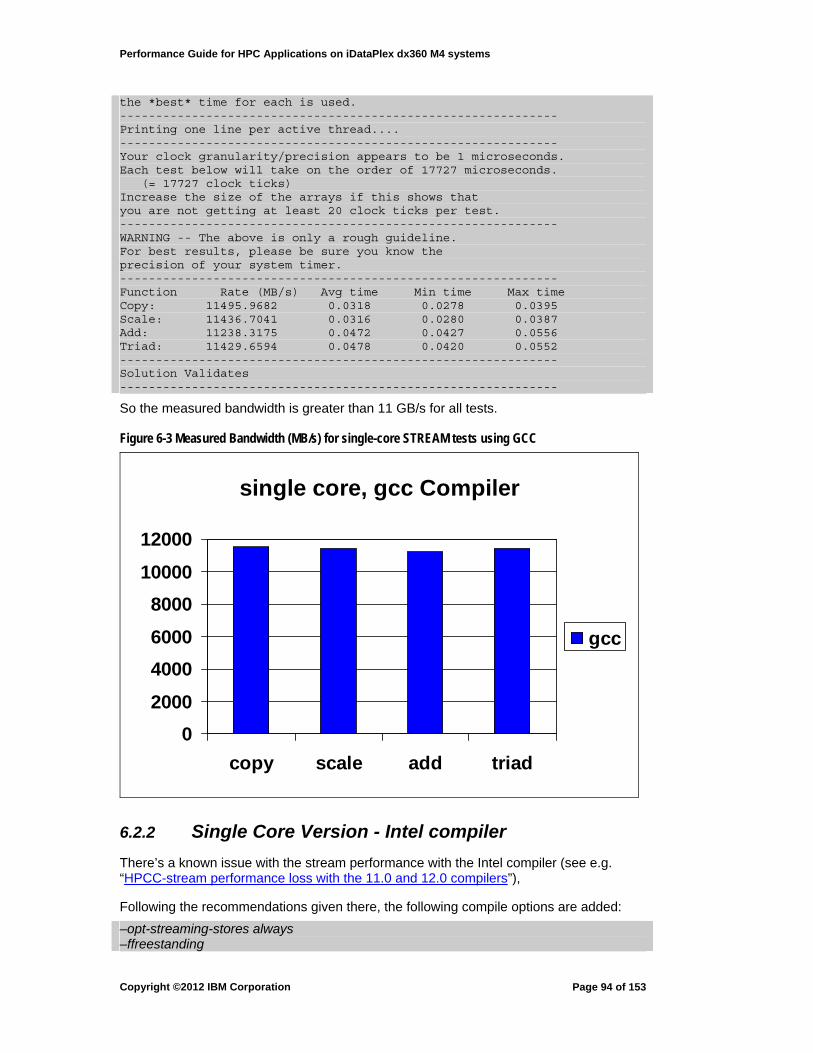
Performance Guide for HPC Applications on iDataPlex dx360 M4 systems
the *best* time for each is used. ------------------------------------------------------------- Printing one line per active thread.... ------------------------------------------------------------- Your clock granularity/precision appears to be 1 microseconds. Each test below will take on the order of 17727 microseconds. (= 17727 clock ticks) Increase the size of the arrays if this shows that you are not getting at least 20 clock ticks per test. ------------------------------------------------------------- WARNING -- The above is only a rough guideline. For best results, please be sure you know the precision of your system timer. ------------------------------------------------------------- Function Rate (MB/s) Avg time Min time Max time Copy: 11495.9682 0.0318 0.0278 0.0395 Scale: 11436.7041 0.0316 0.0280 0.0387 Add: 11238.3175 0.0472 0.0427 0.0556 Triad: 11429.6594 0.0478 0.0420 0.0552 ------------------------------------------------------------- Solution Validates -------------------------------------------------------------
So the measured bandwidth is greater than 11 GB/s for all tests.
Figure 6-3 Measured Bandwidth (MB/s) for single-core STREAM tests using GCC
single core, gcc Compiler
0
2000
4000
6000
8000
10000
12000
copy scale add triad
gcc
6.2.2 Single Core Version - Intel compiler
There’s a known issue with the stream performance with the Intel compiler (see e.g. “HPCC-stream performance loss with the 11.0 and 12.0 compilers”),
Following the recommendations given there, the following compile options are added:
–opt-streaming-stores always –ffreestanding
Copyright ©2012 IBM Corporation
Page 94 of 153

Performance Guide for HPC Applications on iDataPlex dx360 M4 systems
and using the Intel compiler version 12.1.1.256:
# icc -V Intel(R) C Intel(R) 64 Compiler XE for applications running on Intel(R) 64, Version 12.1.1.256 Build 20111011
The following Makefile was used to create binaries from C and Fortran source code:
FC = ifort CC = icc FFLAGS = -O3 -opt-streaming-stores always CFLAGS = -O2 all: stream.exe stream.exe: stream.f mysecond.o $(CC) $(CFLAGS) -c mysecond.c $(FC) $(FFLAGS) -c stream.f $(FC) $(FFLAGS) stream.o mysecond.o -o stream.exe clean: rm -f stream.exe *.o
results in:
------------------------------------------------------------- STREAM version $Revision: 5.9 $ ------------------------------------------------------------- This system uses 8 bytes per DOUBLE PRECISION word. ------------------------------------------------------------- Array size = 20000000, Offset = 0 Total memory required = 457.8 MB. ... ------------------------------------------------------------- Function Rate (MB/s) Avg time Min time Max time Copy: 11572.7884 0.0277 0.0277 0.0277 Scale: 6919.6523 0.0463 0.0462 0.0463 Add: 9040.9096 0.0531 0.0531 0.0531 Triad: 9121.3157 0.0527 0.0526 0.0527 ------------------------------------------------------------- Solution Validates -------------------------------------------------------------
The Intel Fortran compiler yields a result very similar to the Intel C compiler:
... ---------------------------------------------------- Function Rate (MB/s) Avg time Min time Max time Copy: 11581.2764 0.0277 0.0276 0.0277 Scale: 6921.3294 0.0463 0.0462 0.0463 Add: 9045.3372 0.0531 0.0531 0.0531 Triad: 9122.6796 0.0527 0.0526 0.0527 ---------------------------------------------------- Solution Validates! ----------------------------------------------------
Copyright ©2012 IBM Corporation
Page 95 of 153

Performance Guide for HPC Applications on iDataPlex dx360 M4 systems
Figure 6-4 Measured Bandwidth (MB/s) for single-core STREAM tests using Intel icc
single core, Intel compiler
0
2000
4000
6000
8000
10000
12000
copy scale add triad
icc
Comparing the two sets of results shows the binaries produced by the GCC compiler are faster:
Figure 6-5 Measured Bandwidth (MB/s) for single-core STREAM tests comparing Intel icc and GCC
single core
0
2000
4000
6000
8000
10000
12000
copy scale add triad
MB
/s gcc
icc
From a private communication with Andrey Semin from Intel®, changing the compiler
Copyright ©2012 IBM Corporation
Page 96 of 153

Performance Guide for HPC Applications on iDataPlex dx360 M4 systems
options for icc to disable streaming stores alters this picture. Using the options
-diag-disable 161 -O1 -ipo -opt-streaming-stores never -static
produces the result:
------------------------------------------------------------- STREAM version $Revision: 5.9 $ ------------------------------------------------------------- This system uses 8 bytes per DOUBLE PRECISION word. ------------------------------------------------------------- Array size = 20000000, Offset = 0 Total memory required = 457.8 MB. Each test is run 20 times, but only the *best* time for each is used. ------------------------------------------------------------- Printing one line per active thread.... ------------------------------------------------------------- Your clock granularity/precision appears to be 1 microseconds. Each test below will take on the order of 22251 microseconds. (= 22251 clock ticks) Increase the size of the arrays if this shows that you are not getting at least 20 clock ticks per test. ------------------------------------------------------------- WARNING -- The above is only a rough guideline. For best results, please be sure you know the precision of your system timer. ------------------------------------------------------------- Function Rate (MB/s) Avg time Min time Max time Copy: 11507.8948 0.0278 0.0278 0.0279 Scale: 11522.8132 0.0278 0.0278 0.0278 Add: 12349.4306 0.0391 0.0389 0.0415 Triad: 12393.5235 0.0388 0.0387 0.0390 ------------------------------------------------------------- Solution Validates -------------------------------------------------------------
This result with the Intel compiler is faster than the gcc result.
Copyright ©2012 IBM Corporation
Page 97 of 153

Performance Guide for HPC Applications on iDataPlex dx360 M4 systems
Figure 6-6 Measured Bandwidth (MB/s) for single-core STREAM tests comparing Intel icc without streaming stores and GCC
single core
0
2000
4000
6000
8000
10000
12000
copy scale add triad
MB
/s
gcc
icc
icc*
where icc* denotes the results without streaming stores.
6.2.3 Frequency Dependency
Both of the examples above were run at the nominal frequency (2.7 GHz) of the CPU without turbo mode. The cpufreq-info tool outputs:
cpufrequtils 004: cpufreq-info (C) Dominik Brodowski 2004-2006 Report errors and bugs to http://bugs.opensuse.org, please. analyzing CPU 0: driver: acpi-cpufreq CPUs which need to switch frequency at the same time: 0 hardware limits: 1.20 GHz - 2.70 GHz available frequency steps: 2.70 GHz, 2.60 GHz, 2.50 GHz, 2.40 GHz, 2.30 GHz, 2.20 GHz, 2.10 GHz, 2.00 GHz, 1.90 GHz, 1.80 GHz, 1.70 GHz, 1.60 GHz, 1.50 GHz, 1.40 GHz, 1.30 GHz, 1.20 GHz available cpufreq governors: conservative, userspace, powersave, ondemand, performance current policy: frequency should be within 1.20 GHz and 2.70 GHz. The governor "userspace" may decide which speed to use within this range. current CPU frequency is 2.70 GHz.
Switching the frequency to 2.5 GHz (and using the gcc-compiled binary), there is a performance degradation of about 6%, whereas the frequency is 8% lower. So a further investigation of the scaling of bandwidth with frequency seems warranted.
... ------------------------------------------------------------- Function Rate (MB/s) Avg time Min time Max time
Copyright ©2012 IBM Corporation
Page 98 of 153
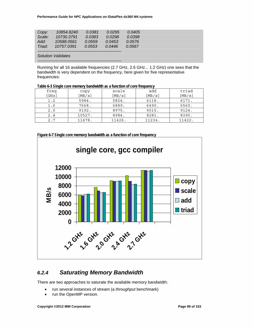
Performance Guide for HPC Applications on iDataPlex dx360 M4 systems
Copy: 10854.8240 0.0381 0.0295 0.0405 Scale: 10730.3791 0.0383 0.0298 0.0398 Add: 10588.0561 0.0559 0.0453 0.0576 Triad: 10757.0391 0.0553 0.0446 0.0567 ------------------------------------------------------------- Solution Validates -------------------------------------------------------------
Running for all 16 available frequencies (2.7 GHz, 2.6 GHz... 1.2 GHz) one sees that the bandwidth is very dependent on the frequency, here given for five representative frequencies:
Table 6-3 Single core memory bandwidth as a function of core frequency freq [GHz]
copy [MB/s]
scale [MB/s]
add [MB/s]
triad [MB/s]
1.2 5984. 5824. 6118. 6171. 1.6 7668. 6889. 6490. 6560. 2.0 9192. 8975. 9015. 9124. 2.4 10527. 8984. 8281. 8390. 2.7 11478. 11426. 11234. 11422.
Figure 6-7 Single core memory bandwidth as a function of core frequency
single core, gcc compiler
02000400060008000
1000012000
1.2 G
Hz
1.6 G
Hz
2.0 G
Hz
2.4 G
Hz
2.7 G
Hz
MB
/s
copy
scale
add
triad
6.2.4 Saturating Memory Bandwidth
There are two approaches to saturate the available memory bandwidth:
• run several instances of stream (a throughput benchmark) • run the OpenMP version.
Copyright ©2012 IBM Corporation
Page 99 of 153
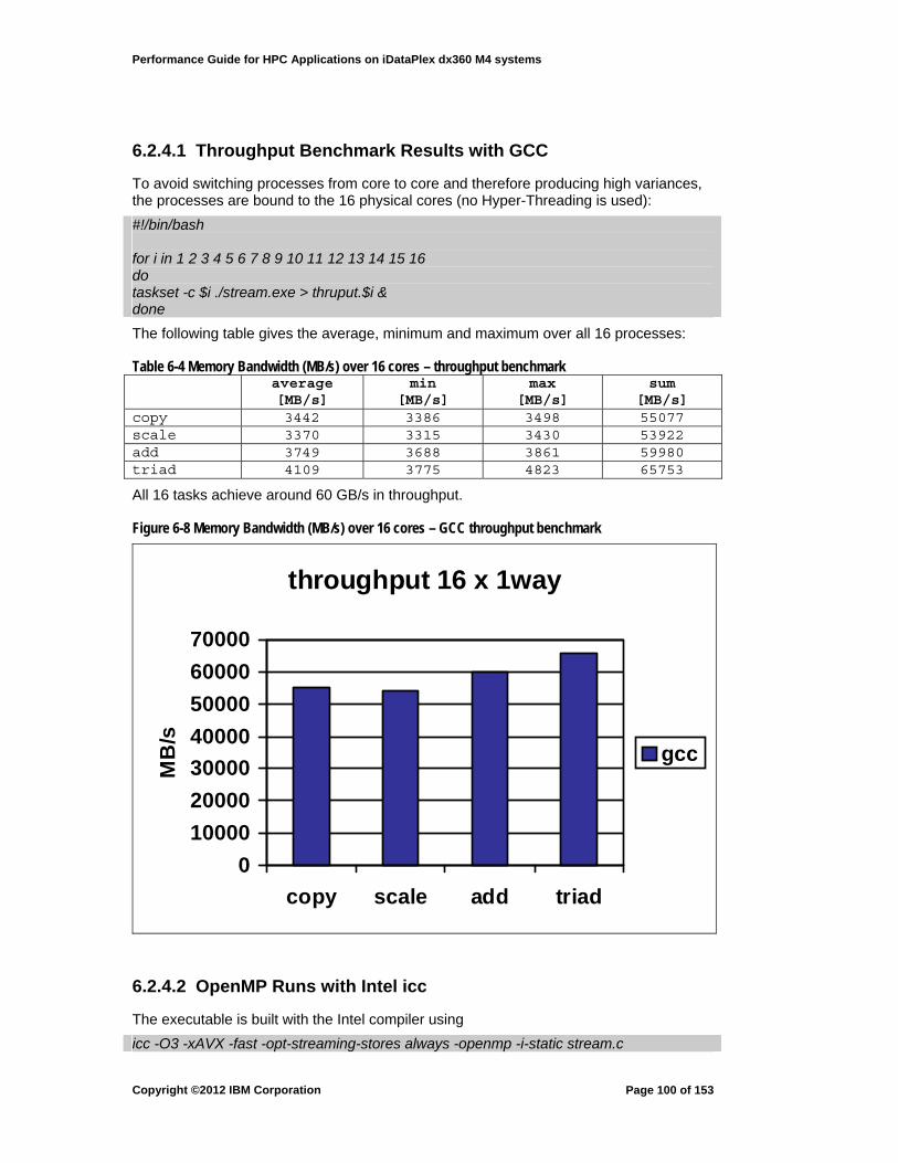
Performance Guide for HPC Applications on iDataPlex dx360 M4 systems
6.2.4.1 Throughput Benchmark Results with GCC
To avoid switching processes from core to core and therefore producing high variances, the processes are bound to the 16 physical cores (no Hyper-Threading is used):
#!/bin/bash for i in 1 2 3 4 5 6 7 8 9 10 11 12 13 14 15 16 do taskset -c $i ./stream.exe > thruput.$i & done
The following table gives the average, minimum and maximum over all 16 processes:
Table 6-4 Memory Bandwidth (MB/s) over 16 cores – throughput benchmark average
[MB/s] min
[MB/s] max
[MB/s] sum
[MB/s] copy 3442 3386 3498 55077 scale 3370 3315 3430 53922 add 3749 3688 3861 59980 triad 4109 3775 4823 65753
All 16 tasks achieve around 60 GB/s in throughput.
Figure 6-8 Memory Bandwidth (MB/s) over 16 cores – GCC throughput benchmark
throughput 16 x 1way
0
10000
20000
30000
40000
50000
60000
70000
copy scale add triad
MB
/s
gcc
6.2.4.2 OpenMP Runs with Intel icc
The executable is built with the Intel compiler using
icc -O3 -xAVX -fast -opt-streaming-stores always -openmp -i-static stream.c
Copyright ©2012 IBM Corporation
Page 100 of 153
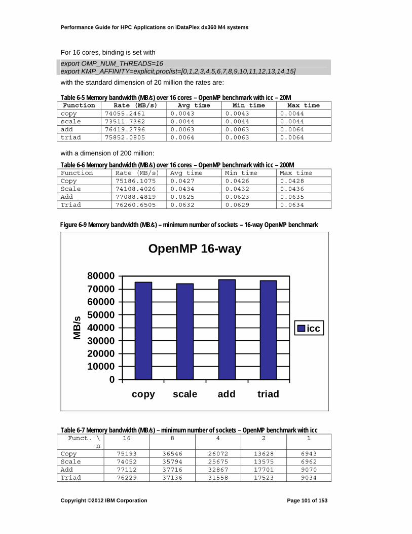
Performance Guide for HPC Applications on iDataPlex dx360 M4 systems
For 16 cores, binding is set with
export OMP_NUM_THREADS=16 export KMP_AFFINITY=explicit,proclist=[0,1,2,3,4,5,6,7,8,9,10,11,12,13,14,15]
with the standard dimension of 20 million the rates are:
Table 6-5 Memory bandwidth (MB/s) over 16 cores – OpenMP benchmark with icc – 20M Function Rate (MB/s) Avg time Min time Max time copy 74055.2461 0.0043 0.0043 0.0044 scale 73511.7362 0.0044 0.0044 0.0044 add 76419.2796 0.0063 0.0063 0.0064 triad 75852.0805 0.0064 0.0063 0.0064 with a dimension of 200 million:
Table 6-6 Memory bandwidth (MB/s) over 16 cores – OpenMP benchmark with icc – 200M Function Rate (MB/s) Avg time Min time Max time Copy 75186.1075 0.0427 0.0426 0.0428 Scale 74108.4026 0.0434 0.0432 0.0436 Add 77088.4819 0.0625 0.0623 0.0635 Triad 76260.6505 0.0632 0.0629 0.0634
Figure 6-9 Memory bandwidth (MB/s) – minimum number of sockets – 16-way OpenMP benchmark
OpenMP 16-way
01000020000300004000050000600007000080000
copy scale add triad
MB
/s
icc
Table 6-7 Memory bandwidth (MB/s) – minimum number of sockets – OpenMP benchmark with icc Funct. \
n 16 8 4 2 1
Copy 75193 36546 26072 13628 6943 Scale 74052 35794 25675 13575 6962 Add 77112 37716 32867 17701 9070 Triad 76229 37136 31558 17523 9034
Copyright ©2012 IBM Corporation
Page 101 of 153

Performance Guide for HPC Applications on iDataPlex dx360 M4 systems
Binding half the threads to one socket and the other half to the other socket the picture improves, especially for 8 cores:
Table 6-8 Memory bandwidth (MB/s) – split threads between two sockets – OpenMP benchmark with icc Funct. \
n 8 4 2
Copy 55375 29288 13662 Scale 54543 29220 13649 Add 69763 37665 17752 Triad 67197 37245 17712
Figure 6-10 Memory bandwidth (MB/s) – performance of 8 threads on 1 or 2 sockets
OpenMP 8-way
01000020000300004000050000600007000080000
copy scale add triad
MB
/s 1 socket
2 sockets
So with Stream
16 cores get ~76 GB/s or 4.75 GB/s per core 8 cores on a single socket ~37 GB/s or 4.63 GB/s per core
8 cores using both sockets ~62 GB/s or 7.7 GB/s per core Figure 6-11 shows the saturation when splitting different numbers of OpenMP threads between both sockets. It reveals that, in general, going from four to eight threads using both sockets scales nicely whereas the memory bandwidth becomes saturated going from 8 to 16 threads.
Copyright ©2012 IBM Corporation
Page 102 of 153

Performance Guide for HPC Applications on iDataPlex dx360 M4 systems
Figure 6-11 Memory bandwidth (MB/s) – split threads between two sockets
OpenMP 2 sockets1 ... 16 threads
0
20000
40000
60000
80000
copy scale add triad
MB
/s
1
2
4
8
16
6.2.4.3 OpenMP Runs with GCC
The corresponding GCC numbers (version 4.3.4) are very different
For 16 cores, binding is set with
export GOMP_CPU_AFFINITY="0 1 2 3 4 5 6 7 8 9 10 11 12 13 14 15")
For 8 cores, binding is set with
export OMP_NUM_THREADS=8 export GOMP_CPU_AFFINITY="0 1 2 3 8 9 10 11"
Table 6-9 Memory bandwidth (MB/s) – minimum number of sockets – OpenMP benchmark with gcc Funct. \
n 16 8 4 2 1
Copy 53102 26539 27309 21356 11723 Scale 53411 26756 27469 20827 11626 Add 60062 30060 30772 23807 12397 Triad 60336 30416 30915 24298 12750
Table 6-10 Memory bandwidth (MB/s) – divide threads between two sockets – OpenMP benchmark with gcc Function 8 4 2
Copy 54450 43233 24226 Scale 54803 42520 24139 Add 61337 48836 26044 Triad 61721 49789 26501
Copyright ©2012 IBM Corporation
Page 103 of 153

Performance Guide for HPC Applications on iDataPlex dx360 M4 systems
6.2.4.4 Saturating Memory Bandwidth — Conclusions
The – rather new – OpenMP support for gcc (and perhaps the version of gcc used) may have had a more negative influence on the performance here as compared to the Intel implementation.
In summary: Memory performance is very dependant on the chosen frequency.
For the single core performance, gcc is clearly ahead of the Intel executable, but for the OpenMP version this picture reverses. Furthermore 8 cores distributed over both sockets can nearly exhaust the memory bandwidth. Binding is absolutely necessary.
6.2.5 Beyond Stream
In the previous section, the simple case of stride-1 loops, where the Sandy Bridge chip really excels, was discussed. In this section, strided operations, loops with a decrement (running the wrong direction through memory) and indexed operations (gathered loads and scattered stores) are investigated.
6.2.5.1 Stride
16 threads by array stride through memory:
Table 6-11 Strided memory bandwidth (MB/s) – 16 threads stride copy scale add triad
2 26195 25832 29003 29290 3 17475 17210 19268 19519 4 13053 12914 14470 14666 5 10505 10301 11558 11634 6 8746 8551 9623 9735 7 7464 7341 8286 8356 8 6558 6431 7246 7329 9 5996 5876 6619 6680 10 5573 5483 6188 6214 20 3641 3563 4095 4071 40 3259 3180 3659 3683
8 threads:
Table 6-12 Strided memory bandwidth (MB/s) – 8 threads stride copy scale add triad
2 13215 13167 14753 14808 3 8837 8784 9843 9921 4 6598 6549 7339 7387 5 5270 5238 5890 5926 6 4399 4381 4897 4916 7 3763 3737 4191 4217 8 3289 3271 3670 3691 9 3027 3000 3370 3380 10 2827 2781 3119 3121 20 1869 1830 2089 2077 40 1683 1650 1891 1884
4 threads
Copyright ©2012 IBM Corporation
Page 104 of 153

Performance Guide for HPC Applications on iDataPlex dx360 M4 systems
Table 6-13 Strided memory bandwidth (MB/s) – 4 threads stride copy scale add triad
2 13557 13586 15042 15146 3 9033 8976 9989 10021 4 6757 6720 7445 7475 5 5399 5362 5943 5979 6 4475 4446 4947 4963 7 3842 3819 4257 4289 8 3350 3333 3720 3735 9 3098 3062 3421 3426 10 2874 2835 3170 3152 20 1878 1831 2069 2044 40 1637 1604 1790 1785
2 threads
Table 6-14 Strided memory bandwidth (MB/s) – 2 threads stride copy scale add triad
2 10472 10715 11495 11932 3 6902 6979 7329 7421 4 5136 5142 5387 5400 5 4064 4092 4324 4307 6 3384 3389 3611 3591 7 2891 2884 3137 3116 8 2511 2522 2741 2745 9 2277 2266 2496 2486 10 2092 2077 2311 2280 20 1383 1377 1480 1482 40 1199 1189 1239 1259
1 thread
Table 6-15 Strided memory bandwidth (MB/s) – 1 thread stride copy scale add triad
2 5736 5908 6015 6106 3 3737 3769 3845 3867 4 2795 2800 2837 2828 5 2203 2213 2275 2257 6 1830 1836 1909 1888 7 1560 1561 1659 1641 8 1351 1352 1448 1444 9 1212 1207 1320 1312 10 1111 1191 1227 1207 20 736 740 793 801 40 656 667 677 691
Figure 6-12 shows, for the triad case, the decrease in effective memory bandwidth as the stride increases.
Copyright ©2012 IBM Corporation
Page 105 of 153

Performance Guide for HPC Applications on iDataPlex dx360 M4 systems
Figure 6-12 Memory bandwidth (MB/s) vs stride length for 1 to 16 threads
strided triad w. OpenMP1 … 16 threads
05000
1000015000200002500030000
2 3 4 5 6 7 8 9 10 20 40
stride
MB
/s
1
2
4
8
16
6.2.5.2 Reverse Order
Stride through memory in reverse order:
Table 6-16 Reverse order (stride=-1) memory bandwidth (MB/s) – 1 to 16 threads Function 16 8 4 2 1
Copy 25653 26703 27324 20812 11562 Scale 25657 26676 27271 20930 11460 Add 28984 30156 30756 23944 12370 Triad 28993 30128 30816 24238 12689
which is in contrast with Table 6-17 for stride 1 memory
Table 6-17 Stride 1 memory bandwidth (MB/s) – 1 to 16 threads Function 16 8 4 2 1
Copy 53102 26539 27309 21356 11723 Scale 53411 26756 27469 20827 11626 Add 60062 30060 30772 23807 12397 Triad 60336 30416 30915 24298 12750
6.2.5.3 Indexed
There are two cases: loads via an index array and stores via an indexed array.
To achieve this another array “index“ is included to modify the stream code, where
index[i] = (ix + iy * i) % N
Copyright ©2012 IBM Corporation
Page 106 of 153

Performance Guide for HPC Applications on iDataPlex dx360 M4 systems
and the offset variable ix and the stride variable iy are read in at runtime.
All results have been generated from binaries created with the Intel compiler.
The results showed that the initial offset ix does not change the performance, so ix = 0 is used for all runs.
load case:
These runs measure the performance of indexed loads - for example, the triad case is modified to become:
for (j=0; j<N; j++) a[j] = b[index[j]]+scalar*c[index[j]];
OMP_NUM_THREADS=1
Table 6-18 Strided memory bandwidth (MB/s) with indexed loads – 1 thread stride copy scale add triad
1 5773 5776 10327 10137 2 5000 5011 6882 6735 3 4291 4284 5185 5049 4 3693 3694 4084 4061 5 3158 3158 3395 3408 6 2737 2738 2942 2955 7 2362 2363 2587 2581 8 2062 2062 2293 2280 9 1899 1898 2114 2091 10 1777 1777 1958 1937
OMP_NUM_THREADS=16
Table 6-19 Strided memory bandwidth (MB/s) with indexed loads – 16 threads stride copy scale add triad
1 52100 51908 49500 49438 2 44120 43960 36057 36097 3 31340 31368 28352 28313 4 33826 33868 31453 31356 5 23580 23583 19623 19613 6 16698 16712 14117 14104 7 16999 17006 13932 13933 8 26357 26378 24269 24554 9 12432 12431 10339 10345 10 11300 11302 9161 9193
store case:
We measure the performance - for example for the triad case -
for (j=0; j<N; j++) a[index[j]] = b[j]+scalar*c[j];
OMP_NUM_THREADS=1
Table 6-20 Strided memory bandwidth (MB/s) with indexed stores – 1 thread stride copy scale add triad
1 9340 9368 10148 10070 2 6107 5992 7486 7445
Copyright ©2012 IBM Corporation
Page 107 of 153

Performance Guide for HPC Applications on iDataPlex dx360 M4 systems
stride copy scale add triad 3 4709 4670 5990 6115 4 3759 3737 4911 4887 5 3139 3142 4213 4197 6 2680 2690 3662 3660 7 2360 2369 3263 3260 8 2091 2091 2920 2915 9 1923 1925 2715 2710 10 1759 1761 2503 2501
OMP_NUM_THREADS=16
Table 6-21 Strided memory bandwidth (MB/s) with indexed stores – 16 threads stride copy scale add triad
1 41807 41915 49940 49967 2 24076 24023 34037 34050 3 19998 19963 27335 27359 4 22477 22465 31790 31830 5 12538 12534 17957 17953 6 9908 9904 14470 14477 7 9050 9056 13174 13177 8 16971 17608 24840 24853 9 7412 7414 10865 10867 10 6691 6693 9838 9836
Observations:
• remember: index[i] = (ix + iy * i) % N • for the case ix = 0, iy = 1 we have the same memory access pattern as for the
standard stream, but for example, the triad case shows 49967 / 76229 = 65.5% of the performance (store case). Whereas – surprisingly – the case OMP_NUM_THREADS=1 gives slightly better performance (comparing results against the Intel compiler).
6.3 HPCC
The HPC Challenge Benchmark is composed of seven individual benchmarks combined into a single executable program, limiting the tuning possibilities for any specific part. It is made up of the following tests:
1. HPL – High Performance Linpack measures the floating-point-execution rate by solving a linear system of equations.
2. PTRANS – Parallel Matrix Transpose measures the network capacity by requiring paired communications across all processors in parallel.
3. DGEMM – (double-precision) General Matrix Multiply measures the floating-point-execution rate by using the corresponding matrix multiplication kernel included in the BLAS library.
4. STREAM measures the sustainable memory bandwidth and corresponding computation rate for simple vector kernels.
5. RandomAccess measures the integer operation rate on random memory locations.
6. FFT – measures the floating-point-execution rate by executing a one-dimensional complex Discrete Fourier Transformation (DFT), which may be implemented using an FFT library.
7. Communication – a combination of tests to measure network bandwidth and latency by simulating various parallel communication patterns.
Copyright ©2012 IBM Corporation
Page 108 of 153
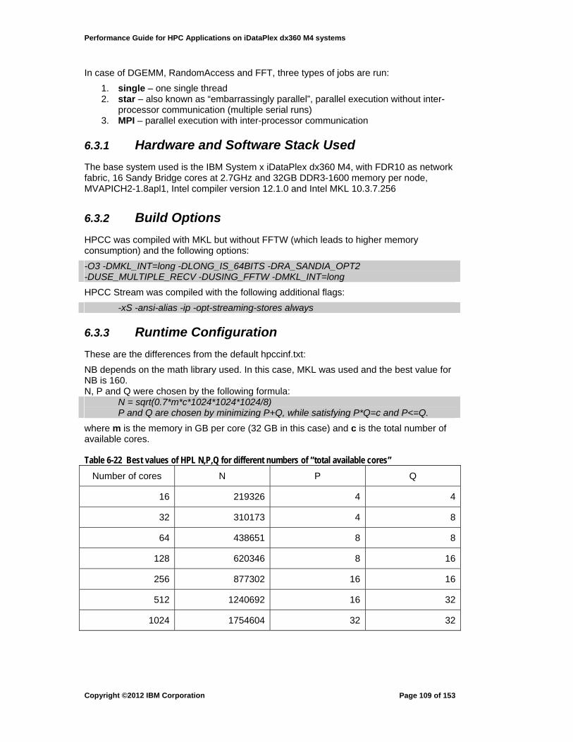
Performance Guide for HPC Applications on iDataPlex dx360 M4 systems
In case of DGEMM, RandomAccess and FFT, three types of jobs are run:
1. single – one single thread 2. star – also known as “embarrassingly parallel”, parallel execution without inter-
processor communication (multiple serial runs) 3. MPI – parallel execution with inter-processor communication
6.3.1 Hardware and Software Stack Used
The base system used is the IBM System x iDataPlex dx360 M4, with FDR10 as network fabric, 16 Sandy Bridge cores at 2.7GHz and 32GB DDR3-1600 memory per node, MVAPICH2-1.8apl1, Intel compiler version 12.1.0 and Intel MKL 10.3.7.256
6.3.2 Build Options
HPCC was compiled with MKL but without FFTW (which leads to higher memory consumption) and the following options:
-O3 -DMKL_INT=long -DLONG_IS_64BITS -DRA_SANDIA_OPT2 -DUSE_MULTIPLE_RECV -DUSING_FFTW -DMKL_INT=long
HPCC Stream was compiled with the following additional flags:
-xS -ansi-alias -ip -opt-streaming-stores always
6.3.3 Runtime Configuration
These are the differences from the default hpccinf.txt:
NB depends on the math library used. In this case, MKL was used and the best value for NB is 160. N, P and Q were chosen by the following formula: N = sqrt(0.7*m*c*1024*1024*1024/8) P and Q are chosen by minimizing P+Q, while satisfying P*Q=c and P<=Q.
where m is the memory in GB per core (32 GB in this case) and c is the total number of available cores.
Table 6-22 Best values of HPL N,P,Q for different numbers of “total available cores”
Number of cores N P Q
16 219326 4 4
32 310173 4 8
64 438651 8 8
128 620346 8 16
256 877302 16 16
512 1240692 16 32
1024 1754604 32 32
Copyright ©2012 IBM Corporation
Page 109 of 153

Performance Guide for HPC Applications on iDataPlex dx360 M4 systems
6.3.4 Results
Table 6-23 HPCC performance on 1 to 32 nodes
Cores (16 per node)
16 32 64 128 256
HPL in TFLOP/s
0.299 0.591 1.166 2.312 4.480
PTRANS in GB/s
5.173 9.745 12.093 23.296 42.947
DGEMM in GFLOP/s
Single 20.238 20.16 20.232 20.269 20.207
Star 19.783 18.64 19.275 19.362 19.605
Single Stream in GB/s
Copy 7.584 7.606 7.603 7.539 7.535
Scale 7.600 7.618 7.615 7.549 7.546
Add 9.820 9.843 9.834 9.745 9.739
Triad 9.789 9.811 9.796 9.710 9.707
Star Stream in GB/s
Copy 4.680 4.693 4.841 4.746 4.713
Scale 4.608 4.618 4.793 4.703 4.632
Add 4.882 4.889 5.375 5.134 4.883
Triad 4.817 4.818 5.369 5.098 4.819
RandomAccess in GUP/s
Single 0.035 0.035 0.035 0.035 0.035
Star 0.018 0.018 0.018 0.018 0.018
MPI 0.177 0.301 0.495 0.763 1.262
FFT in GFLOP/s
Single 3.500 3.552 3.534 3.530 3.561
Star 2.842 2.630 2.464 2.521 2.593
MPI 19.58 24.833 41.435 74.95 147.63
PingPong Latency in us
Min 0.367 0.517 0.775 0.951 0.876
Avg 0.866 1.233 1.534 1.967 2.134
Max 2.517 2.293 2.724 3.838 2.962
PingPong Bandwidth in GB/s
Copyright ©2012 IBM Corporation
Page 110 of 153

Performance Guide for HPC Applications on iDataPlex dx360 M4 systems
Cores (16 per node)
16 32 64 128 256
Min 3.696 3.41 2.895 2.886 3.081
Avg 5.545 4.856 4.589 4.578 4.549
Max 7.753 7.381 7.067 7.106 7.767
Ring Bandwidth in GB/s, NOR: Natural Order, ROR: Random Order
NOR 1.332 1.325 1.316 1.274 1.281
ROR 1.036 0.574 0.322 0.241 0.202
Ring Latency in us, NOR: Natural Order, ROR: Random Order
NOR 1.230 1.295 2.027 2.113 1.999
ROR 1.316 1.685 3.247 6.896 10.348
6.4 NAS Parallel Benchmarks Class D
The NAS Parallel Benchmark suite consists of five kernels and three pseudo-applications, derived from computational fluid dynamics (CFD) simulations. There are three versions of the benchmark suite, based on the communications method(s) used: MPI, OpenMP, and hybrid (MPI/OMP); some kernels do not use all communications methods. Each part tries to mimic the computation and data-access patterns found in CFD applications and no modifications or external libraries may be used. Problem sizes are predefined by classes.
Kernels:
• CG – Conjugate Gradient, irregular memory access and communication • MG – Multi-Grid V-Cycle, long- and short-distance communication, memory
intensive • FT – (Fast) Fourier Transformation solving a partial differential equation (PDE) in
3D space, all-to-all communication • Pseudo-applications to solve nonlinear PDEs using the following algorithms: • BT – Block Tri-diagonal solver, non-blocking communication • SP – Scalar Penta-diagonal solver, non-blocking communication • LU – Lower-Upper Gauss-Seidel solver
6.4.1 Hardware and Building
The base system used is the IBM System x iDataPlex dx360 M4, with FDR10 as network fabric, 16 Sandy Bridge cores at 2.7GHz and 32GB DDR3-1600 memory per node, MVAPICH2-1.8apl1, Intel compiler version 12.1.0 and Intel MKL 10.3.7.256
Compilation was done directly on a Sandy Bridge node with the following flags:
-O3 -xAVX -xhost
In case of class E with small process count, the following flags were added:
-mcmodel=medium -shared-intel
Copyright ©2012 IBM Corporation
Page 111 of 153

Performance Guide for HPC Applications on iDataPlex dx360 M4 systems
6.4.2 Results
Results are in total giga-operations per second with class D problem size:
Table 6-24 NAS PB Class D performance on 1 to 32 nodes CG MG FT LU BT SP
64 19.573 99.798 135.32 103.09 49.270128 34.372 184.10 98.066 263.89 242.79 93.878256 66.608 387.80 205.55 496.17 529.1 256.3 484 1003.4 509.1
Num
ber
of
core
s
512 117.03 829.17 342.83 868.1
Copyright ©2012 IBM Corporation
Page 112 of 153

Performance Guide for HPC Applications on iDataPlex dx360 M4 systems
7 AVX and SIMD Programming
7.1 AVX/SSE SIMD Architecture
Intel® Advanced Vector eXtensions (AVX), is an extension to the venerable Intel64 architecture that supports Single Instruction Multiple Data (SIMD) operations on Intel® architectures starting with Sandy Bridge. The new instruction set introduced with AVX is the natural follow-on to the previous SIMD architecture, SSE4. AVX defines additional registers and instructions to support single-instruction multiple-data (SIMD) operations that accelerate data-intensive tasks.
The Intel64 SIMD hardware and instruction set support for previous architectures has
• 8 architected 64-bit (MMX) and 16 architected 128-bit (SSE) registers • arithmetic, bit-shuffling and logical operations for
1-, 2-, 4-, and 8-byte integers 4- and 8-byte floating point data
The AVX floating point architecture adds the following new capabilities:
• Wider Vectors The 16 128-bit registers (named XMM0-15) have been extended to 32 bytes (256 bits). The new architected registers are named YMM0-15. They can hold 8 single-precision or 4 double-precision floating point values.
Figure 7-1 Using the low 128-bits of the YMMn registers for XMMn
YMM0XMM0
• Three and four operand operations nondestructive source operands for AVX 128 and AVX 256 operations A = B + C can be used instead of A = A + B
• Increased memory bandwidth An additional 128-bit load port 2 load ports and 1 store port read up to 32 bytes and write 16 bytes per cycle
• Unaligned memory access support • New instructions
focusing on SIMD instructions for 32-bit and 64-bit floating point data AVX can work on either 128-bit or 256-bit vector data AVX-128 instructions replace the complete SSE instruction set. Instructions using the XMMn registers use the lower 128 bits. The upper 128 bits are zeroed out.
Vector technology provides a software model that accelerates the performance of various software applications and extends the instruction set architecture (ISA) of the Intel® Core CPU architecture. The instruction set is based on separate vector/SIMD-style execution units that have a high degree of data parallelism. This high data parallelism can perform operations on multiple data elements in a single instruction.
7.1.1 Note on Terminology:
The term “vector”, as used in this chapter, refers to the spatial parallel processing of
Copyright ©2012 IBM Corporation
Page 113 of 153
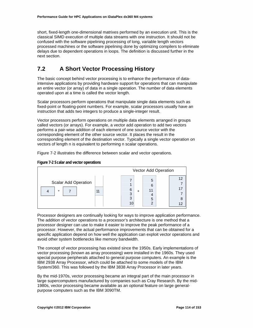
Performance Guide for HPC Applications on iDataPlex dx360 M4 systems
short, fixed-length one-dimensional matrixes performed by an execution unit. This is the classical SIMD execution of multiple data streams with one instruction. It should not be confused with the software pipelining processing of long, variable length vectors processed machines or the software pipelining done by optimizing compilers to eliminate delays due to dependent operations in loops. The definition is discussed further in the next section.
7.2 A Short Vector Processing History
The basic concept behind vector processing is to enhance the performance of data-intensive applications by providing hardware support for operations that can manipulate an entire vector (or array) of data in a single operation. The number of data elements operated upon at a time is called the vector length.
Scalar processors perform operations that manipulate single data elements such as fixed-point or floating-point numbers. For example, scalar processors usually have an instruction that adds two integers to produce a single-integer result.
Vector processors perform operations on multiple data elements arranged in groups called vectors (or arrays). For example, a vector add operation to add two vectors performs a pair-wise addition of each element of one source vector with the corresponding element of the other source vector. It places the result in the corresponding element of the destination vector. Typically a single vector operation on vectors of length n is equivalent to performing n scalar operations.
Figure 7-2 illustrates the difference between scalar and vector operations.
Figure 7-2 Scalar and vector operations
Vector Add Operation
+ 7
11
7 16 3 310
+
5 6
11 4 5
2
Scalar Add Operation
4
12 7
17 7 8
12
Processor designers are continually looking for ways to improve application performance. The addition of vector operations to a processor’s architecture is one method that a processor designer can use to make it easier to improve the peak performance of a processor. However, the actual performance improvements that can be obtained for a specific application depend on how well the application can exploit vector operations and avoid other system bottlenecks like memory bandwidth.
The concept of vector processing has existed since the 1950s. Early implementations of vector processing (known as array processing) were installed in the 1960s. They used special purpose peripherals attached to general purpose computers. An example is the IBM 2938 Array Processor, which could be attached to some models of the IBM System/360. This was followed by the IBM 3838 Array Processor in later years.
By the mid-1970s, vector processing became an integral part of the main processor in large supercomputers manufactured by companies such as Cray Research. By the mid-1980s, vector processing became available as an optional feature on large general-purpose computers such as the IBM 3090TM.
Copyright ©2012 IBM Corporation
Page 114 of 153

Performance Guide for HPC Applications on iDataPlex dx360 M4 systems
In the 1990s, developers of microprocessors used in desktop computers adapted the concept of vector processing to enhance the capability of their microprocessors when running desktop multimedia applications. These capabilities were usually referred to as Single Instruction Multiple Data (SIMD) extensions and operated on short vectors. Examples of other SIMD extensions in widespread use today include:
Intel® Multimedia Extensions (MMXTM)
Intel® Streaming SIMD Extensions (SSE)
AMD 3DNow!
Motorola AltiVec and IBM VMX/AltiVec
IBM VSX
The SIMD extensions found in microprocessors used in desktop computers operate on short vectors of length 2, 4, 8, or 16. This is in contrast to the classic vector supercomputers that can often exploit long vectors of length 64 or more.
Copyright ©2012 IBM Corporation
Page 115 of 153
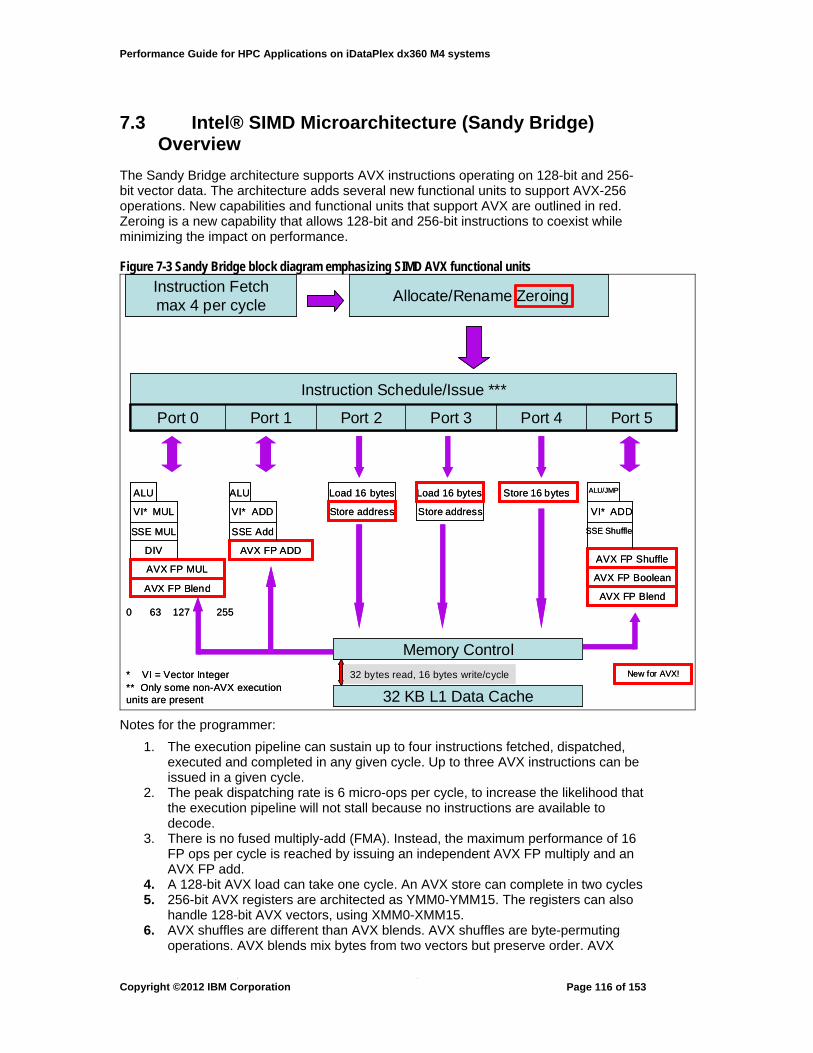
Performance Guide for HPC Applications on iDataPlex dx360 M4 systems
7.3 Intel® SIMD Microarchitecture (Sandy Bridge) Overview
The Sandy Bridge architecture supports AVX instructions operating on 128-bit and 256-bit vector data. The architecture adds several new functional units to support AVX-256 operations. New capabilities and functional units that support AVX are outlined in red. Zeroing is a new capability that allows 128-bit and 256-bit instructions to coexist while minimizing the impact on performance.
Figure 7-3 Sandy Bridge block diagram emphasizing SIMD AVX functional units
Instruction Fetchmax 4 per cycle
Allocate/Rename Zeroing
Instruction Schedule/Issue ***
Port 5Port 4Port 3Port 2Port 1Port 0
AVX FP Blend
AVX FP MUL
DIV
SSE MUL
VI* MUL
ALU
0 63 127 255
AVX FP ADD
SSE Add
VI* ADD
ALU
AVX FP Boolean
AVX FP Blend
AVX FP Shuffle
SSE Shuffle
VI* ADD
ALU/JMP
Store address
Load 16 bytes Store 16 bytes
Memory Control
32 KB L1 Data Cache
32 bytes read, 16 bytes write/cycle
Store address
Load 16 bytes
New for AVX!* VI = Vector Integer** Only some non-AVX execution units are present
Notes for the programmer:
1. The execution pipeline can sustain up to four instructions fetched, dispatched, executed and completed in any given cycle. Up to three AVX instructions can be issued in a given cycle.
2. The peak dispatching rate is 6 micro-ops per cycle, to increase the likelihood that the execution pipeline will not stall because no instructions are available to decode.
3. There is no fused multiply-add (FMA). Instead, the maximum performance of 16 FP ops per cycle is reached by issuing an independent AVX FP multiply and an AVX FP add.
4. A 128-bit AVX load can take one cycle. An AVX store can complete in two cycles 5. 256-bit AVX registers are architected as YMM0-YMM15. The registers can also
handle 128-bit AVX vectors, using XMM0-XMM15. 6. AVX shuffles are different than AVX blends. AVX shuffles are byte-permuting
operations. AVX blends mix bytes from two vectors but preserve order. AVX
Copyright ©2012 IBM Corporation
Page 116 of 153

Performance Guide for HPC Applications on iDataPlex dx360 M4 systems
shuffles are only executed by Port 5, so minimize the number of times shuffles are needed.
7. Integer SSE instructions are only supported as 128-bit AVX instructions. 8. There is a 1 cycle penalty to move data from the INT stack to the FP stack. 9. AVX supports unaligned memory accesses, but the performance is better when
accessing 32-byte aligned data.
7.4 Vectorization Overview
So, repeating the point of section 7.2, the reason to care about vector technology is performance. Vector technology can provide dramatic performance gains, up to 8 times the best scalar performance for some cases.
So how does SIMD code differ from scalar code? Compare the code fragments from examples 7-1 and 7-2.
Example 7-1 Scalar vector addition float *a, *b, *c; ... for ( i = 0, i < n, i++) { a[i] = b[i] + c[i]; // scalar version }
Example 7-2 Vectorization of scalar addition #include <immintrin.h> float *a, *b, *c; __m256 va, vb, vc; ... for ( i = 0, i < n / vector_size, i+=8) { va = _mm256_loadu_ps(&a[i]); vb = _mm256_loadu_ps(&b[i]); vc = _mm256_add_ps(va,vb); _mm_256_storeu_ps(&c[i],vc); }
In example 7-2, the 32-bit scalar data type has been replaced by a vector data type, __m256. The vector data has to be explicitly loaded from and stored back into scalar arrays. Note that the loop range is no longer n iterations, but is reduced by the vector data type length (vector_size = 8 for floats when using AVX). Remember, an AVX vector register can hold 256 bits (32 bytes) of data. Therefore, the vector addition operation
vc = _mm256_add_ps(va,vb);
can execute 8 add operations with a single instruction for each vector, as opposed to multiple scalar instructions. The vectorized version can be up to 8 times faster than the scalar version.
Intel AVX functionality targets a diverse set of applications in the following areas:
• Video editing/ post production • Audio processing • Image processing • Animation • Bioinformatics • A broad range of scientific applications in physics and chemistry. • A broad range of engineering applications dedicated to solving the partial
Copyright ©2012 IBM Corporation
Page 117 of 153

Performance Guide for HPC Applications on iDataPlex dx360 M4 systems
differential equations of their respective fields.
7.5 Auto-vectorization
Translating scalar code into vector intrinsics is beyond the scope of this discussion. However, it is relatively straightforward to get the Intel compilers to automatically vectorize code and report on which loops have been vectorized. The recommended options are:
For C/C++:
icc –O3 –xAVX –vec-report1 –vec-report2
For Fortran:
ifort –O3 –xAVX –vec-report1 –vec-report2
These options would be used in addition to other optimization options, such as -finline or –opt-streaming-stores.
• –xAVX, is the option that explicitly asks the compiler to auto-vectorize loops with AVX instructions. The compiler will try auto-vectorization by default at optimization levels –O2 and above.
• -vec-report1 reports when the compiler has vectorized a loop • -vec-report2 provides reasons about why the compiler failed to vectorize a
loop #define ITER 10 void foo(int size) { int i, j; float *x, *y, *a; int iter_count=1024; ... ... for (j = 0; j < ITER; j++){ for (i = 0; i < iter_count; i+=1){ x[i] = y[i] + a[i+1]; } } }
After building a program with auto-vectorization, program performance should be tested. If the performance is not as expected, a programmer can refer to comments in the listing provided by –-vec-report2 to identify reasons for loops that failed to auto-vectorize and give the programmer direction on how to correct code to auto-vectorize properly.
7.6 Inhibitors of Auto-vectorization
Here are some common conditions which can prevent the compiler from performing auto-vectorization.
7.6.1 Loop-carried Data Dependencies
In the presence of loop-carried data dependences where data is read after it is written, auto-vectorization cannot be carried out. As shown in the simple code snippet below, in
Copyright ©2012 IBM Corporation
Page 118 of 153

Performance Guide for HPC Applications on iDataPlex dx360 M4 systems
every iteration i of the loop, c[i-1] is being read which is written in the i-1th iteration. When such a loop is transformed using AVX instructions it results in incorrect values being computed in the c array.
for (i = 0; i < N; i++) c[i] = c[i-1] + 1
Certain compiler transformations applied to loops may help resolve certain kinds of loop-carried data dependences and enable auto-vectorization.
7.6.2 Memory Aliasing
When loops contain data which can potentially overlap, the compiler may desist from auto-vectorization as it can lead to incorrect results. For the code snippet shown below, if the memory locations of the pointers a, b, and c denoted by a[0..N-1], b[0..N-1] and c[0..N-1] do not overlap, and the compiler can statically deduce this fact, the loop will be vectorized and AVX instructions generated for it. However, in general, it may be non-trivial for the compiler to deduce this at compile-time and subsequently the loop may remain serial. This can happen even when in reality the memory locations do not overlap.
double foo(double *a, double *b, double *c) { for (i = 0; i < N; i++) a[i] = b[i] + c[i] }
The user can help the compiler resolve the memory aliasing issues by telling the compiler when memory is disjoint using: #pragma ivdep
For the example above, adding
#pragma ivdep double foo(double *a, double *b, double *c) { for (i = 0; i < N; i++) a[i] = b[i] + c[i] }
will enable the compiler to make safe assumptions about the aliasing and subsequently vectorize the loop.
The compiler may, in certain situations ( where memory overlap pragmas are not provided or the compiler cannot safely analyze overlaps), generate versioned code to compute the overlap at runtime i.e. it inserts code to test for memory overlap and generates auto-vectorized or serial code based on whether the test passes or fails at runtime.
7.6.3 Non-stride-1 Accesses
For auto-vectorization to happen, usually, the compiler expects the accesses of the data to happen from contiguous locations in memory (what we refer to as stride-1 accesses) so that once the vector stores and loads happen, the resultant data can be fed directly to the computation operands. However, with non stride-1 accesses, data may not be loaded or stored from contiguous locations, leading to several complexities in code generation. Even if the non-contiguous loading/storing pattern is known, the compiler would now need to generate certain extra instructions to pack/unpack the data into vector registers before they can be operated upon. These extra instructions (not present in the serial
Copyright ©2012 IBM Corporation
Page 119 of 153
Performance Guide for HPC Applications on iDataPlex dx360 M4 systems
code) may increase the cost of implementing auto-vectorization and the compiler may pre-empt the decision to auto-vectorize those loops based on heuristic/profile-driven cost analyses. In the code snippet shown below, the accesses of array b[] are non-unit strides, since another array, idx[], is used to index into b[]. The compiler does not auto-vectorize such a loop.
for (i = 0; i < N; i++) a[i] = b[idx[i]]
7.6.4 Other Vectorization Inhibitors in Loops
A loop which is a candidate for auto-vectorization may exhibit one or more of the following characteristics which may inhibit vectorization.
• contains flow control: (restricted form of if/then/else allowed) for ( i = 0; i < n ; i++) { if ( i < 8 ) c[i] = a[i] + b[i]; else c[i] = a[i] - b[i]; }
This kind of flow control is handled by the compiler by splitting the loop into two separate loops and vectorizing them:
for ( i = 0; i < 8 ; i++) { c[i] = a[i] + b[i] }
and
for ( i = 8; i < n ; i++) { c[i] = a[i] - b[i] }
• trip count is too small : short loops are not worth vectorizing
• contains a function call:
o embedded function calls may be eliminated with the C compiler option -finline)
7.6.5 Data Alignment
For auto-vectorization, the compiler tries to ensure that vector loads/stores are from aligned memory locations to minimize the misalignment penalty as much as possible. The most common sorts of alignment issues come from array malloc()s:
a = (float *) malloc(arraylen*sizeof(float));
The portable way to force alignment on 32-byte boundaries is with posix_memalign()
posix_memalign((void **)&a,32,arraylen*sizeof(float));
The Intel C Compiler also provides its own method of aligning malloc()’d data, which has its own associated free() function, too.
a = (float *) _mm_malloc (arraylen*sizeof(float),32); _mm_free (a);
Copyright ©2012 IBM Corporation
Page 120 of 153

Performance Guide for HPC Applications on iDataPlex dx360 M4 systems
These are less portable, and can’t be interchanged with malloc() and free().
Copyright ©2012 IBM Corporation
Page 121 of 153

Performance Guide for HPC Applications on iDataPlex dx360 M4 systems
7.7 Additional References
For additional information about the topics presented in this chapter, the interested reader can refer to
[1] How to Optimize for AVX [2] AVX Software Development Tools and Libraries [3] Introduction to Intel AVX [4] Practical AVX Optimization [5] Intel Math Kernel Library Documentation [6] Intel Integrated Performance Primitives Documentation [7] Intel Fortran Compiler XE 12.1 User and Reference Guide [8] Introduction to Vectorization with Intel C++ Compiler [9] Introduction to Vectorization with Intel Fortran [10] Auto-vectorization with Intel C++ compilers [11] A Guide to Auto-vectorization with Intel C++ Compilers [12] Intel C++ auto-vectorization tutorial
Copyright ©2012 IBM Corporation
Page 122 of 153

Performance Guide for HPC Applications on iDataPlex dx360 M4 systems
8 Hardware Accelerators
8.1 GPGPUs
The Graphics Processing Unit (GPU) has evolved into a highly parallel, multithreaded many core processor with exceptional compute power and with very high local memory bandwidth. Originally, GPUs were designed for 3-D rendering of large sets of pixels, and vertices mapped naturally to parallel threads. Many high performance computing (HPC) applications are capable of taking advantage of these threads in the GPUs. Both NVIDIA and AMD with Fusion/ATI have been offering these GPUs for high performance computing applications for the last four years. GPUs that can be used for HPC applications are commonly referred to as “GPGPUs” (General Purpose GPUs).
IBM has been selling NVIDIA GPUs in the iDataPlex and bladeserver nodes since 2011. There has been a lot of interest from customers on GPU based servers.
The purpose of this chapter is to examine the role of GPUs on IBM iDataPlex systems, details of the GPUs, the software available for GPUs, and programming the GPUs for performance. This chapter discusses how to run HPL with GPUs, and the tools available for GPU performance.
8.1.1 NVIDIA Tesla 2090 Hardware description
NVIDIA developed CUDA (a hardware, and software architecture that enables NVIDIA Graphics Processing Units or GPUs) to execute user-developed programs in C, C++, FORTRAN, OpenCL, DirectCompute and other languages. A CUDA program invokes parallel kernels, where a kernel executes in parallel across a set of threads. A detailed description of CUDA hardware may be found in [1]. A brief description is included here to explain some of the concepts.
A kernel is a set of computations that can be executed in parallel by a single core of a GPGPU. Each instance of the kernel is executed in a single thread that has its own private memory, thread ID, program counter, and registers. A thread block is a set of concurrently executing threads that can cooperate among themselves through barrier synchronization and shared memory. A thread block has a block ID within its grid.
A grid is an array of thread blocks that executes the same kernel, reads inputs from global memory, writes results to global memory, and synchronizes between dependent kernel calls.
Each thread block has a per-Block shared memory space used for inter-thread communication, data sharing, and result sharing in parallel algorithms. Grids of thread blocks share results in Global memory space after kernel-wide global synchronization.
CUDA’s hierarchy of threads maps to a hierarchy of processors on the GPU; The GPU executes one or more kernel threads; a streaming multiprocessor (SM) executes one or more thread blocks; and CUDA cores and other execution units in the SM execute threads. The SM executes threads in groups of 32 threads called a warp.
Copyright ©2012 IBM Corporation
Page 123 of 153

Performance Guide for HPC Applications on iDataPlex dx360 M4 systems
Copyright ©2012 IBM Corporation
Page 124 of 153
There are 512 CUDA cores, and these are organized into 16 SMs of 32 cores each. The GPU has 64-bit memory partitions, for a 384-bit memory interface supporting a total of 6 GB of GDDR5 DRAM memory. A host interface connects the GPU to the CPU via PCI-Express. The GigaThread global scheduler distributes thread blocks to the SM thread scheduler. Figure 8-1 shows the GPU layout for the Fermi GPU (the code name for the latest Tesla product as of March 2012). One of the SMs is outlined in red.
Figure 8-1 Functional block diagram of the Tesla Fermi GPU
D
RA
M I/
F
DR
AM
I/F
HO
ST
I/F
DR
AM
I/F
L2
G
iga
Thr
ead
DR
AM
I/F
DR
AM
I/F
DR
AM
I/F

Performance Guide for HPC Applications on iDataPlex dx360 M4 systems
Figure 8-2 shows a block diagram of the Fermi Streaming Multiprocessor (SM). Each SM has16 load/store units. (It can load data for 16 threads at a time.) There are 4 Special Function Units (SFUs) for functions such as sine, cosine, reciprocal, and square root. And each SM has a fundamental computational block of 32 CUDA cores. One CUDA core is outlined in red.
Figure 8-2 Tesla Fermi SM block diagram
Instruction Cache Scheduler Scheduler
Dispatch Dispatch
Register File
Core Core Core Core Core Core Core Core Core Core Core Core Core Core Core Core Core Core Core Core
Core Core Core Core
Core Core Core Core Core Core Core Core
16 Load/Store Units
4 Special Funct Units
Network Interconnect
64K Local Shared Memory
Uniform Cache
Copyright ©2012 IBM Corporation
Page 125 of 153
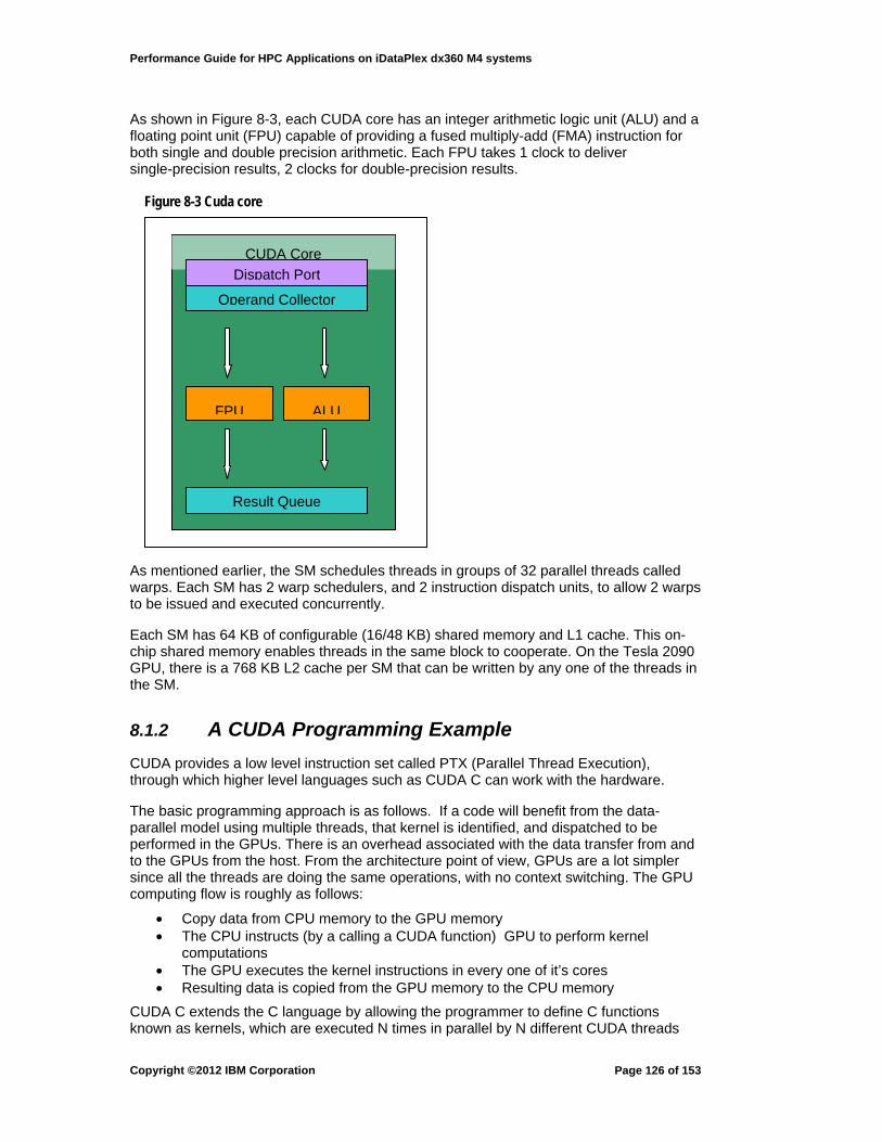
Performance Guide for HPC Applications on iDataPlex dx360 M4 systems
As shown in Figure 8-3, each CUDA core has an integer arithmetic logic unit (ALU) and a floating point unit (FPU) capable of providing a fused multiply-add (FMA) instruction for both single and double precision arithmetic. Each FPU takes 1 clock to deliver single-precision results, 2 clocks for double-precision results.
Figure 8-3 Cuda core
CUDA Core
Dispatch Port
Operand Collector
Result Queue
FPU ALU
As mentioned earlier, the SM schedules threads in groups of 32 parallel threads called warps. Each SM has 2 warp schedulers, and 2 instruction dispatch units, to allow 2 warps to be issued and executed concurrently.
Each SM has 64 KB of configurable (16/48 KB) shared memory and L1 cache. This on-chip shared memory enables threads in the same block to cooperate. On the Tesla 2090 GPU, there is a 768 KB L2 cache per SM that can be written by any one of the threads in the SM.
8.1.2 A CUDA Programming Example
CUDA provides a low level instruction set called PTX (Parallel Thread Execution), through which higher level languages such as CUDA C can work with the hardware.
The basic programming approach is as follows. If a code will benefit from the data-parallel model using multiple threads, that kernel is identified, and dispatched to be performed in the GPUs. There is an overhead associated with the data transfer from and to the GPUs from the host. From the architecture point of view, GPUs are a lot simpler since all the threads are doing the same operations, with no context switching. The GPU computing flow is roughly as follows:
• Copy data from CPU memory to the GPU memory • The CPU instructs (by a calling a CUDA function) GPU to perform kernel
computations • The GPU executes the kernel instructions in every one of it’s cores • Resulting data is copied from the GPU memory to the CPU memory
CUDA C extends the C language by allowing the programmer to define C functions known as kernels, which are executed N times in parallel by N different CUDA threads
Copyright ©2012 IBM Corporation
Page 126 of 153
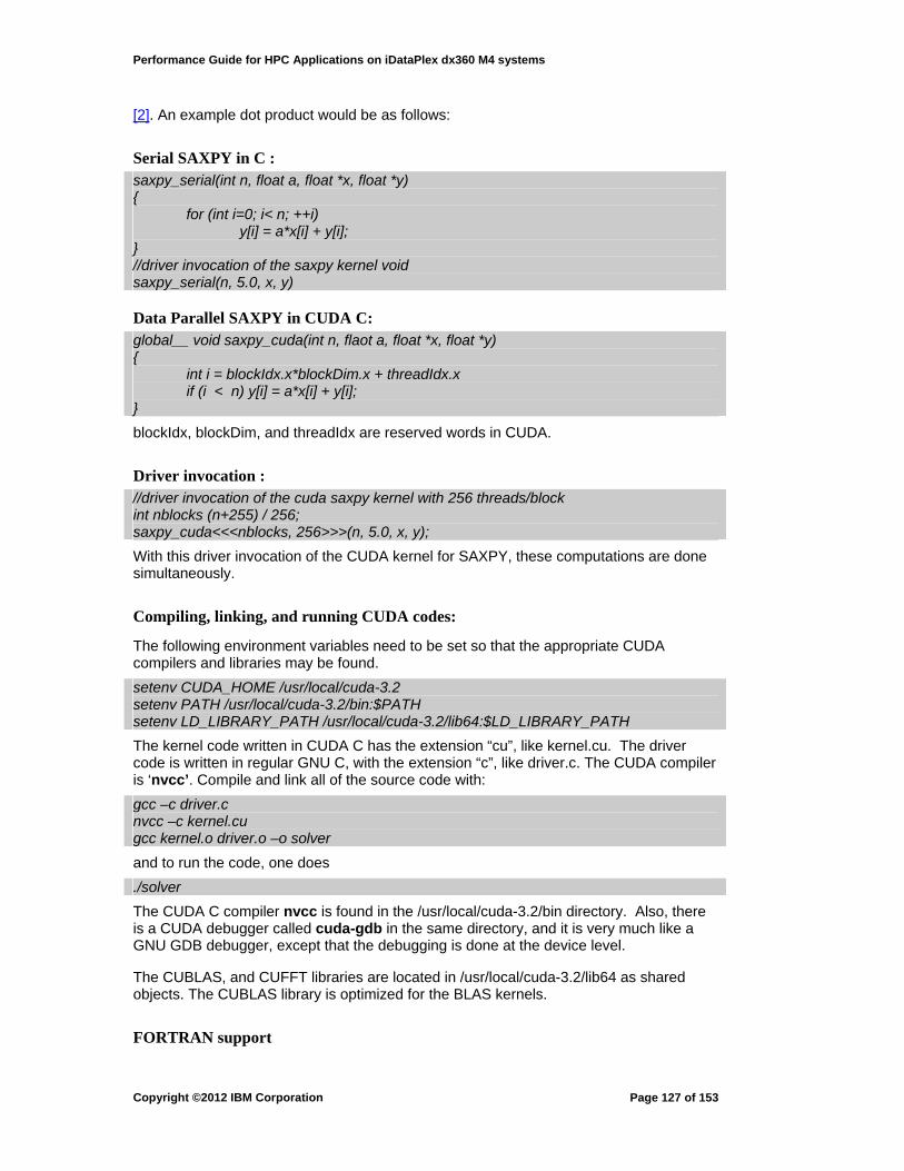
Performance Guide for HPC Applications on iDataPlex dx360 M4 systems
[2]. An example dot product would be as follows:
Serial SAXPY in C : saxpy_serial(int n, float a, float *x, float *y) { for (int i=0; i< n; ++i) y[i] = a*x[i] + y[i]; } //driver invocation of the saxpy kernel void saxpy_serial(n, 5.0, x, y)
Data Parallel SAXPY in CUDA C: global__ void saxpy_cuda(int n, flaot a, float *x, float *y) { int i = blockIdx.x*blockDim.x + threadIdx.x if (i < n) y[i] = a*x[i] + y[i]; }
blockIdx, blockDim, and threadIdx are reserved words in CUDA.
Driver invocation : //driver invocation of the cuda saxpy kernel with 256 threads/block int nblocks (n+255) / 256; saxpy_cuda<<<nblocks, 256>>>(n, 5.0, x, y);
With this driver invocation of the CUDA kernel for SAXPY, these computations are done simultaneously.
Compiling, linking, and running CUDA codes:
The following environment variables need to be set so that the appropriate CUDA compilers and libraries may be found.
setenv CUDA_HOME /usr/local/cuda-3.2 setenv PATH /usr/local/cuda-3.2/bin:$PATH setenv LD_LIBRARY_PATH /usr/local/cuda-3.2/lib64:$LD_LIBRARY_PATH
The kernel code written in CUDA C has the extension “cu”, like kernel.cu. The driver code is written in regular GNU C, with the extension “c”, like driver.c. The CUDA compiler is ‘nvcc’. Compile and link all of the source code with:
gcc –c driver.c nvcc –c kernel.cu gcc kernel.o driver.o –o solver
and to run the code, one does
./solver
The CUDA C compiler nvcc is found in the /usr/local/cuda-3.2/bin directory. Also, there is a CUDA debugger called cuda-gdb in the same directory, and it is very much like a GNU GDB debugger, except that the debugging is done at the device level.
The CUBLAS, and CUFFT libraries are located in /usr/local/cuda-3.2/lib64 as shared objects. The CUBLAS library is optimized for the BLAS kernels.
FORTRAN support
Copyright ©2012 IBM Corporation
Page 127 of 153

Performance Guide for HPC Applications on iDataPlex dx360 M4 systems
PGI provides support for GPUs with multiple mechanisms. There is a CUDA C, and CUDA FORTRAN from PGI. In addition, there is support through directives, in the PGI Accelerator model. These are very similar to OpenMP directives for parallelization [3].
There is also a CAPS HMPP compiler that provides support for FORTRAN codes [4].
8.1.3 Memory Hierarchy in GPU Computations
Figure 8-4 NVIDIA GPU memory hierarchy
Figure 8-4 shows the basic memory hierarchy of the NVIDIA GPUs. To reiterate — each SM has a 64 KB L1 cache on chip, and 768 KB L2 cache off chip; there is a 6 GB global GPU memory; and the GPU has a PCI-express interface to the system. The data transfer rates vary widely in CUDA computing:
• with in the device (50-80 GB/sec) • asynchronous host-to-device with pinned memory (10-20 GB/sec) • PCIe transfer rate (4-6 GB/sec)
Because of the small size of the caches, and the possibility of memory bank conflicts, CUDA programming strongly discourages any cache blocking when tuning for performance. The desired tuning procedure is known as memory coalescing. The details of this may be found in the NVIDIA tutorials. Here is an example of memory coalescing in CUDA for a 2-D transpose [5].
In the naïve transpose, loads are coalesced; stores are not (the stride runs over the column index). In addition, there are other read-only memories, known as texture memory and constant memory, available in the GPUs.
Copyright ©2012 IBM Corporation
Page 128 of 153

Performance Guide for HPC Applications on iDataPlex dx360 M4 systems
__global__ void transposeNaive(float *odata, float *idata, int width, int height) { int xIndex = blockIdx.x * blockDim.x + threadIdx.x; //Convert thread indices to int yIndex = blockIdx.y * blockDim.y + threadIdy.y; //coordinates in matrix int index_in = xIndex + width * yIndex; // Convert matrix coordinates int index_out = yIndex + height * xIndex; // to flattened array indices odata[index_out] = idata[index_in] }
In the coalesced method using shared memory, there are two steps:
1. transpose the submatrix into Shared Memory 2. Write rows of the transposed submatrix back to global memory
And the resulting code looks like this:
__global__ void transposeCoalesced(float *odata, float *idata, int width, int height) { __shared__ float tile[TILE_DIM][TILE_DIM+1]; int xIndex = blockIdx.x * TILE_DIM + threadIdx.x; int yIndex = blockIdx.y * TILE_DIM + threadIdx.y; int index_in = xIndex + (yIndex)*width; tile[threadIdx.y][threadIdx.x] = idata[index_in]; --syncthreads(); xIndex = blockIdx.y * TILE_DIM + threadIdx.x; yIndex = blockIdx.x * TILE_DIM + threadIdx.y; int index_out = xIndex + (yIndex)*height; odata[index_out] = tile[threadIdx.x][threadIdx.y]; }
This requires thread synchronization, so that all columns are written to shared memory, before rows are written back to global memory. It also requires that the tile be a perfect square so that threadId.x and threadId.y have same range (TILE_DIM).
In addition to memory coalescing, there are other memory optimization procedures like using texture memory and execution configuration (determining the best thread block dimension). In [6], implementation of the Himeno benchmark that solves the 3-D Poisson equation is discussed with the details of optimizing for performance on GPUs. Using finite-differences, the Poisson equation is discretized in space yielding a 19-point stencil. The discretized equations are solved iteratively using Jacobi relaxation. This benchmark is designed to run with various problem sizes to fit the system. On the Himeno code, optimized for GPUs, memory coalescing gives a 57% performance improvement. Use of Texture cache improves the performance by an additional 33%. Other optimizations (removing logic, and branching) improve the performance by an additional 18% [6].
8.1.4 CUDA Best practices
From the Tuning document for Fermi [7], the recommended best practices may be summarized as
• find ways to parallelize sequential code • minimize data transfers between the host and the device • adjust kernel launch configuration to maximize device utilization • ensure global memory accesses are coalesced • replace global memory access with shared memory access whenever possible
Copyright ©2012 IBM Corporation
Page 129 of 153

Performance Guide for HPC Applications on iDataPlex dx360 M4 systems
• avoid different execution paths within the same warp
8.1.5 Running HPL with GPUs
HPL ([8]) on GPUs is one of the most requested benchmarks for systems with GPUs. There are certain requirements that are important for performance, and those are discussed here. The HPL-GPU code is provided by NVIDIA, and latest version is version 11. There is a problem with Intel MPI that limits scaling, so it is recommended that HPL-GPU be built with OpenMPI. It is preferable to use GNU compilers and Intel MKL libraries to get the best performance.
This example illustrates a case where 2 Tesla M2070 GPGPUs are attached to each 12-core Intel Westmere node. These are some of runtime environmental variables
CPU_CORES_PER_GPU=6 export MKL_NUM_THREADS=$CPU_CORES_PER_GPU export OMP_NUM_THREADS=$CPU_CORES_PER_GPU export CUDA_DGEMM_SPLIT=0.85 export CUDA_DTRSM_SPLIT=0.75
The last 2 environmental variables distribute the work load between the CPUs and the GPUs.
There is a significant impact with processor binding on the performance. With OpenMPI, use of ‘rankfile’ is an effective binding tool.
The HPL-GPU code on the CPU side is a hybrid parallel code. It is best run with a command like this:
$ mpirun -machinefile host.list -np 8 --mca btl_openib_flags 1 -- rankfile rankfile $HPL_DIR/bin/CUDA_pinned/xhpl | tee out_8
where the rankfile looks like this :
rank 0=i04n201 slot=0,1,2,3,4,5 rank 1=i04n201 slot=6,7,8,9,10,11 rank 2=i04n202 slot=0,1,2,3,4,5 rank 3=i04n202 slot=6,7,8,9,10,11 rank 4=i04n203 slot=0,1,2,3,4,5 rank 5=i04n203 slot=6,7,8,9,10,11 rank 6=i04n204 slot=0,1,2,3,4,5 rank 7=i04n204 slot=6,7,8,9,10,11
Also, it is important to choose the right problem size for peak performance. This is generally based on the available node memory, as recommended in the HPL download site ([8]).
The following table shows GPU HPL performance on a customer system that has 2 GPUs per node on 32 nodes with 48 GB of memory per node.
Table 8-1 HPL performance on GPUs # of nodes # of GPUs N (matrix size) Gflops/s 1 2 70000 699 2 4 90000 1299 4 8 130000 2475 8 16 186000 4708 16 32 288168 9090 32 64 409168 18390
Copyright ©2012 IBM Corporation
Page 130 of 153
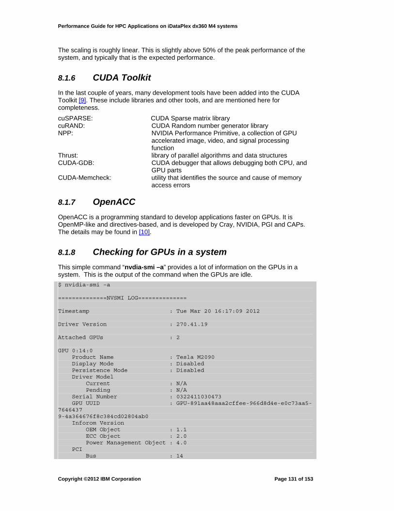
Performance Guide for HPC Applications on iDataPlex dx360 M4 systems
The scaling is roughly linear. This is slightly above 50% of the peak performance of the system, and typically that is the expected performance.
8.1.6 CUDA Toolkit
In the last couple of years, many development tools have been added into the CUDA Toolkit [9]. These include libraries and other tools, and are mentioned here for completeness.
cuSPARSE: CUDA Sparse matrix library cuRAND: CUDA Random number generator library NPP: NVIDIA Performance Primitive, a collection of GPU
accelerated image, video, and signal processing function
Thrust: library of parallel algorithms and data structures CUDA-GDB: CUDA debugger that allows debugging both CPU, and
GPU parts CUDA-Memcheck: utility that identifies the source and cause of memory
access errors
8.1.7 OpenACC
OpenACC is a programming standard to develop applications faster on GPUs. It is OpenMP-like and directives-based, and is developed by Cray, NVIDIA, PGI and CAPs. The details may be found in [10].
8.1.8 Checking for GPUs in a system
This simple command “nvdia-smi –a” provides a lot of information on the GPUs in a system. This is the output of the command when the GPUs are idle.
$ nvidia-smi –a ==============NVSMI LOG============== Timestamp : Tue Mar 20 16:17:09 2012 Driver Version : 270.41.19 Attached GPUs : 2 GPU 0:14:0 Product Name : Tesla M2090 Display Mode : Disabled Persistence Mode : Disabled Driver Model Current : N/A Pending : N/A Serial Number : 0322411030473 GPU UUID : GPU-891aa48aaa2cffee-966d8d4e-e0c73aa5-7646437 9-4a364676f8c384cd02804ab0 Inforom Version OEM Object : 1.1 ECC Object : 2.0 Power Management Object : 4.0 PCI Bus : 14
Copyright ©2012 IBM Corporation
Page 131 of 153

Performance Guide for HPC Applications on iDataPlex dx360 M4 systems
Device : 0 Domain : 0 Device Id : 109110DE Bus Id : 0:14:0 Fan Speed : N/A Memory Usage Total : 6143 Mb Used : 10 Mb Free : 6132 Mb Compute Mode : Default Utilization Gpu : 0 % Memory : 0 % Ecc Mode Current : Disabled Pending : Disabled ECC Errors Volatile Single Bit Device Memory : 0 Register File : 0 L1 Cache : 0 L2 Cache : 0 Total : 0 Double Bit Device Memory : 0 Register File : 0 L1 Cache : 0 L2 Cache : 0 Total : 0 Aggregate Single Bit Device Memory : 0 Register File : 0 L1 Cache : 0 L2 Cache : 0 Total : 0 Double Bit Device Memory : 0 Register File : 0 L1 Cache : 0 L2 Cache : 0 Total : 0 Temperature Gpu : N/A Power Readings Power State : P12 Power Management : Supported Power Draw : 32.58 W Power Limit : 225 W Clocks Graphics : 50 MHz SM : 100 MHz Memory : 135 MHz
Similarly, it provides information for the second GPU with bus Id labeled as 0:15:0.
If the GPUs are being used, under “Utilization”, it will show the GPU and the GPU-memory utilization details in percentages which change dynamically as the program runs on the GPUs.
Copyright ©2012 IBM Corporation
Page 132 of 153

Performance Guide for HPC Applications on iDataPlex dx360 M4 systems
Copyright ©2012 IBM Corporation
Page 133 of 153
8.1.9 References [1] NVIDIA Fermi Compute Architecture [2] NVIDIA CUDA C Programming Guide [3] PGI CUDA Fortran Compiler [4] CAPS [5] NVIDIA Tutorials – Fundamentals of Performance Optimization on Fermi – 2011 [6] Philiips, Everett, and Fatica, Massimiliano, “Implementing Himeno Benchmark with
CUDA on GPU Clusters”, 2010 IEEE Symposium on Parallel and Distributed Processing, April 2010.
[7] Tuning CUDA Applications for Fermi, Version 1.2, NVIDIA, July 2010. [8] HPL at Netlib.org [9] NVIDIA CUDA Toolkit 4.0 [10] NVIDIA OpenACC [11] The Tech Report: “Nvidia’s Fermi GPU architecture revealed”
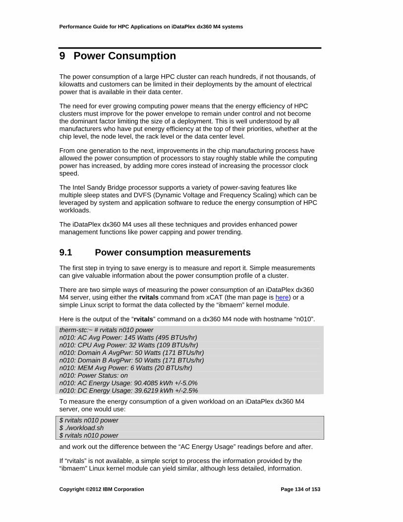
Performance Guide for HPC Applications on iDataPlex dx360 M4 systems
9 Power Consumption
The power consumption of a large HPC cluster can reach hundreds, if not thousands, of kilowatts and customers can be limited in their deployments by the amount of electrical power that is available in their data center.
The need for ever growing computing power means that the energy efficiency of HPC clusters must improve for the power envelope to remain under control and not become the dominant factor limiting the size of a deployment. This is well understood by all manufacturers who have put energy efficiency at the top of their priorities, whether at the chip level, the node level, the rack level or the data center level.
From one generation to the next, improvements in the chip manufacturing process have allowed the power consumption of processors to stay roughly stable while the computing power has increased, by adding more cores instead of increasing the processor clock speed.
The Intel Sandy Bridge processor supports a variety of power-saving features like multiple sleep states and DVFS (Dynamic Voltage and Frequency Scaling) which can be leveraged by system and application software to reduce the energy consumption of HPC workloads.
The iDataPlex dx360 M4 uses all these techniques and provides enhanced power management functions like power capping and power trending.
9.1 Power consumption measurements
The first step in trying to save energy is to measure and report it. Simple measurements can give valuable information about the power consumption profile of a cluster.
There are two simple ways of measuring the power consumption of an iDataPlex dx360 M4 server, using either the rvitals command from xCAT (the man page is here) or a simple Linux script to format the data collected by the “ibmaem” kernel module.
Here is the output of the “rvitals” command on a dx360 M4 node with hostname “n010”.
therm-stc:~ # rvitals n010 power n010: AC Avg Power: 145 Watts (495 BTUs/hr) n010: CPU Avg Power: 32 Watts (109 BTUs/hr) n010: Domain A AvgPwr: 50 Watts (171 BTUs/hr) n010: Domain B AvgPwr: 50 Watts (171 BTUs/hr) n010: MEM Avg Power: 6 Watts (20 BTUs/hr) n010: Power Status: on n010: AC Energy Usage: 90.4085 kWh +/-5.0% n010: DC Energy Usage: 39.6219 kWh +/-2.5%
To measure the energy consumption of a given workload on an iDataPlex dx360 M4 server, one would use:
$ rvitals n010 power $ ./workload.sh $ rvitals n010 power
and work out the difference between the “AC Energy Usage” readings before and after.
If “rvitals” is not available, a simple script to process the information provided by the “ibmaem” Linux kernel module can yield similar, although less detailed, information.
Copyright ©2012 IBM Corporation
Page 134 of 153

Performance Guide for HPC Applications on iDataPlex dx360 M4 systems
Provided the “ibmaem” kernel module is loaded (modprobe ibmaem), one could use this script:
$ cat nrg.sh #!/bin/bash v=1 if [ ! -r /sys/devices/platform/aem.1 ] ; then v=0 fi BDC=`cat /sys/devices/platform/aem.$v/energy1_input` BAC=`cat /sys/devices/platform/aem.$v/energy2_input` b=$(date "+%s%N") $* e=$(date "+%s%N") ADC=`cat /sys/devices/platform/aem.$v/energy1_input` AAC=`cat /sys/devices/platform/aem.$v/energy2_input` RT=$(echo "($e-$b)/1000000"|bc) DC=$((ADC – BDC) AC=$((AAC - BAC) DCP=$(echo "$DC/1000/$RT"|bc -l|cut -d'.' -f1) ACP=$(echo "$AC/1000/$RT"|bc -l|cut -d'.' -f1) echo "Energy: $(( (DC) / 1000000 ))J (DC) Time:$RT (ms) AvgPower: ${DCP}W (DC)" echo "Energy: $(( (AC) / 1000000 ))J (AC) Time:$RT (ms) AvgPower: ${ACP}W (AC)"
9.2
9.3
Performance versus Power Consumption
The following conclusions can be deduced from measuring the power consumption of a compute node:
• Partially loaded systems consume a high fraction of the maximum power. It is not uncommon to see an idle node consume half of the power consumption of a fully loaded node.
• The power consumption of a given system is a monotonic function of the CPU clock frequency.
• The power consumption of a given system depends on the application that is being run. If Linpack HPL is generally considered as a worst case, there are applications which consume far less power.
• The CPU power consumption is the biggest part of the node power but moving data to and from memory is also significant.
• The energy consumption of a given workload (product of the average power consumption and the job's run time) is a complex function of the CPU clock frequency. In some situations it can be beneficial, energy-wise, to run a job at the highest possible clock speed. Granted, the instantaneous power consumption will be higher, but this will be for a shorter period, resulting in an overall energy saving.
The above points show that there are opportunities to reduce the power consumption of compute nodes while minimizing the impact on compute performance.
System Power states
Several power states exist in the system. These power states allow components of the server or the entire server to reduce power consumption and optimize efficiency. The power states are used both when the system is idle and when it is running.
With any of the power-saving states, there is a tradeoff between power savings and
Copyright ©2012 IBM Corporation
Page 135 of 153
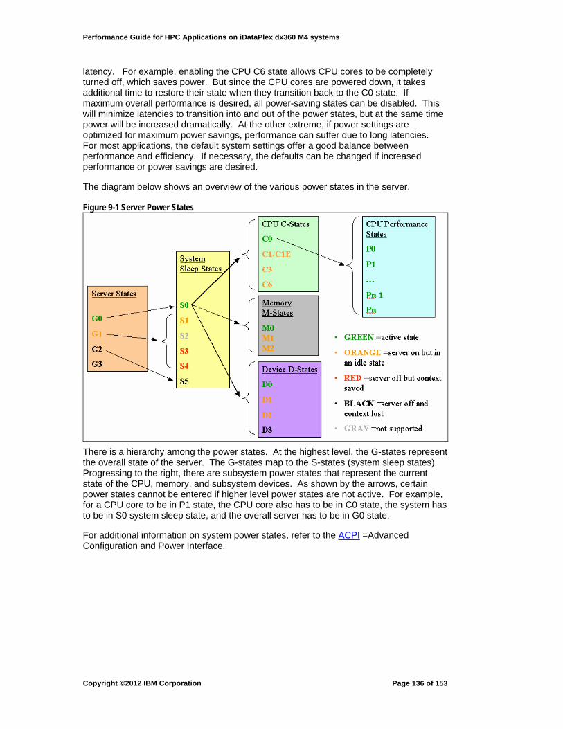
Performance Guide for HPC Applications on iDataPlex dx360 M4 systems
latency. For example, enabling the CPU C6 state allows CPU cores to be completely turned off, which saves power. But since the CPU cores are powered down, it takes additional time to restore their state when they transition back to the C0 state. If maximum overall performance is desired, all power-saving states can be disabled. This will minimize latencies to transition into and out of the power states, but at the same time power will be increased dramatically. At the other extreme, if power settings are optimized for maximum power savings, performance can suffer due to long latencies. For most applications, the default system settings offer a good balance between performance and efficiency. If necessary, the defaults can be changed if increased performance or power savings are desired.
The diagram below shows an overview of the various power states in the server.
Figure 9-1 Server Power States
There is a hierarchy among the power states. At the highest level, the G-states represent the overall state of the server. The G-states map to the S-states (system sleep states). Progressing to the right, there are subsystem power states that represent the current state of the CPU, memory, and subsystem devices. As shown by the arrows, certain power states cannot be entered if higher level power states are not active. For example, for a CPU core to be in P1 state, the CPU core also has to be in C0 state, the system has to be in S0 system sleep state, and the overall server has to be in G0 state.
For additional information on system power states, refer to the ACPI =Advanced Configuration and Power Interface.
Copyright ©2012 IBM Corporation
Page 136 of 153

Performance Guide for HPC Applications on iDataPlex dx360 M4 systems
9.3.1 G-States
G-states are global server states that define the operational state of the entire server. As the number of the G-state increases, there is additional power saved. However, as shown below, the latency to move back to G0 state also increases.
Table 9-1 Global server states G-State Can Applications
Run? OS Reboot Required?
Description
G0 Yes No Server is fully on but some individual components could be in a power-savings state.
G1 No No Standby, suspend, or hibernate modes. See S-states.
G2 No Yes System is in a soft-off state. For example, the power switch was pressed. System draws power from the auxiliary power rail. The main power rail may or may not be switched off.
G3 No Yes AC power is removed. Server is only being powered by the backup battery for RTC, CMOS, and wake events.
HIGHER
LATENCY
HIGHER
POWER
Copyright ©2012 IBM Corporation
Page 137 of 153

Performance Guide for HPC Applications on iDataPlex dx360 M4 systems
9.3.2 S-States
S-states define the sleep state of the entire system. The table below describes the various sleep states.
Table 9-2 Sleep states S-State G-State BIOS
Reboot Required
OS Reboot Required
Relative Power
Relative Latency
Description
S0 G0 No No 6X 0 System is fully on but some components could be in a power-savings state.
S1 G1 No No 2.5X 1% A.K.A “Idle”, “Standby” –if S3 not supported. Typically, when the OS is idle, it will halt the CPU and blank the monitor to save power. No power rails are switched off. This state may go away on future servers.
S2 G1 No No CPU caches are powered down. No known server or OS supports this state.
S3 G1 No No 1.1X 10% A.K.A “Standby”, “Suspend-to-RAM”. The state of the chipset registers is saved to system memory and memory is placed in a low-power self-refresh state. To preserve the memory contents, power is supplied to the DRAMs in S3 state.
S4 G1 Yes No X 90% A.K.A “Hibernate”, “Suspend-to-disk”. The state of the operating system (all memory contents and chip registers) is saved to a file on the HDD and the server is placed in a soft-off state.
S5 G2 Yes Yes X 100% Server is in a soft off state. When turned back on, the server must completely reinitialize with POST and the operating system.
Just as with G-states, higher numbered sleep states save more power but there is additional latency when the system transitions back to S0 state. The middle state, S3, offers a good compromise between power savings and latency.
9.3.3 C-States
C-states are CPU idle power-saving states. C-states higher than C0 only become active when a CPU core is idle. If a process is running on a CPU core, the core is always in C0 state. If Hyper-Threading is enabled, the C-state resolves down to the physical core. For example, if one Hyper-Thread is active and another Hyper-Thread is idle on the same core, the core will remain in C0 state.
C-states can operate on each core separately or the entire CPU package. The CPU
Copyright ©2012 IBM Corporation
Page 138 of 153

Performance Guide for HPC Applications on iDataPlex dx360 M4 systems
package is the physical chip in which the CPU cores reside. It includes the CPU cores, caches, memory controllers, PCI Express interfaces, and miscellaneous logic. The non-CPU core hardware inside the package is commonly referred to as the “uncore”.
Core C-states transitions are driven by interrupts or the operating system scheduler with MWAIT commands. The number of cores in C3 or C6 also impacts the maximum turbo frequency that is available. If maximum peak performance is desired, all CPU C-states should be enabled.
Package C-state transitions are autonomous. No OS awareness or intervention is required. The package C-state is equal to the lowest numbered C-state that any of the CPU cores is in at that point in time. Additional logic inside the CPU package monitors all of the CPU cores and places the package into the appropriate C-state.
Note that CPU C-states do not directly map to ACPI C-states. The reason for this is historical. ACPI C-states range from C0 to C3. At the time when they were defined, there were no CPUs that supported the C6 state. So the mapping was 1:1 (ACPI C0 =CPUC0, ACPI C1=CPU C1, etc.). Newer CPUs, however, support the C6 state. In order to get the maximum power savings when going to the ACPI C3 state, the CPU C6 state gets mapped to ACPI C3 and the CPU C3 state gets mapped to ACPI C2.
Table 9-3 CPU idle power-saving states ACPI C-State CPU C-State C0 C0 C1 C1 C2 C3 C3 C6
Copyright ©2012 IBM Corporation
Page 139 of 153

Performance Guide for HPC Applications on iDataPlex dx360 M4 systems
Shown below is a description of each core and package C-state.
Table 9-4 CPU idle states for each core and socket C-State CPU Core
Description CPU Core Power / Latency Approximations4
CPU Package Description
CPU Package Power / Latency4
C0 • Core is fully on and executing code
• L1 cache coherent
• Core power is on
100% at Pn / 0 nS • At least one core is in C0 state.
100% / 0 nS
C1 • Core is halted
• L1 cache coherent
• Core power is on
30% / 5uS NA –core only state NA
C1E NA –package only NA
mbered
t
ltage
kage will
50% / ~5uS • At least one core isin C1 state and allothers are in a higher nuC-state.
All cores running a•lowest frequency
• VRD5 switches tominimal vostate.
• PLL is on
• CPU pacprocess bus snoops
state
C3
d to cache
stopped
• Core power is on
10% / 50uS
d all re in higher
imal
t is inaccessible. CPU package is not snoopable
25% / ~50uS • Core is halted
• L1 cache flushelast level
• All core clocks
• At least one core is in C3 state anothers anumbered C-states.
• VRD5 in minvoltage state
PLL is off. •• Memory is placed
in self-refresh.
• L3 shared cache retains context bu
4 The number of C-states and the specific power savings associated with each C-state is dependent on the
specific type and SKU of CPU installed. 5 VRD stands for the voltage regulator device
Copyright ©2012 IBM Corporation
Page 140 of 153
Performance Guide for HPC Applications on iDataPlex dx360 M4 systems
C-State CPU Core Description
CPU Core Power / Latency Approximations4
CPU Package CPU Description Package
Power / Latency4
C6 • L1 flushed to LLC
• Core power is off
0% / 100uS • All cores are in C6 state.
• Same power-saving features as package C3 plus some additional uncore savings.
16% / ~100uS
9.3.4 P-States
P-states are defined as the CPU performance states. Each CPU core supports multiple P-states and each P-state corresponds to a frequency. Note, that P0 can run above the rated frequency for short periods of time if turbo mode is enabled. The exact turbo frequency for P0 and the amount of time the core runs at the turbo frequency is controlled autonomously in hardware.
Like core C-states, P-states are controlled by the operating system scheduler. The OS scheduler places a CPU core in a specific P-state depending on the amount of performance needed to complete the current task. For example, if a 2GHz CPU core only needs to run at 1GHz to complete a task, the OS scheduler will place the CPU into a higher numbered P-state.
Each CPU core can be placed in a different P-state. Multiple threads on one core (e.g. Hyper-Threading) are resolved to a single P-state. P-states are only valid when the CPU core is in the C0 state. P-states are sometimes referred to as DVFS (dynamic voltage and frequency scaling) or EIST (Enhanced Intel Speedstep® Technology).
Table 9-5 CPU Performance states P-State CPU Frequency Approximations Description P0 100 to ~130% (with turbo) CPU can run at rated frequency indefinitely or at
turbo frequency (greater than rate frequency) for short periods of time.
P1 ~90 to 95% Intermediate P-state . . . Pn-1 ~85 to 95% Intermediate P-state Pn 1.2 GHz Minimum frequency that CPU core can execute
code.
The exact frequency breakdown for the P-states varies with the rated frequency and power of the CPU used.
In addition to controlling the core frequency, P-states also indirectly control the voltage level of the VRD (voltage regulator device) that is supplying power to the CPU cores. As the core frequency is reduced from its maximum value, the VRD voltage is automatically reduced down to a certain point. Eventually, the VRD will be operating at the minimum voltage that the CPU cores can tolerate. If the core frequency is lowered beyond this point, the VRD voltage will remain at the minimum voltage. This is illustrated in the diagram below.
Copyright ©2012 IBM Corporation
Page 141 of 153

Performance Guide for HPC Applications on iDataPlex dx360 M4 systems
Figure 9-2 The effect of VRD voltage
CPU voltage at a minimum here
Frequency scaling only
Frequency & voltage scaling
Typically, the most efficient operating point is at the peak of the curve.
9.3.5 D-States
D-states are subsystem power-saving states. They are applicable to devices such as LAN, SAS, and USB. The operating system can transition to different D-states after a period of time or when requested by a device driver. All D-states occur when the server is in S0 state.
Table 9-6 Subsystem power states D-State Device Power Device Context Description D0 On Active Device is fully on. All devices support D0
by default even they don’t implement the PCI Power Management specification.
D1 On Active Immediate power state. Lower power consumption than D0. Exact power-saving details are device specific.
D2 On Active Immediate power state. Lower power consumption than D1. Exact power-saving details are device specific.
D3 hot (ACPI D2) On Lost Power to device is left on but the device is placed in a low power state. Device is unresponsive to bus requests.
D3 cold (ACPI D3) Off Lost Power to device is completely removed. All devices support D3 by default even if they don’t implement the PCI Power Management specification.
Copyright ©2012 IBM Corporation
Page 142 of 153

Performance Guide for HPC Applications on iDataPlex dx360 M4 systems
9.3.6 M-States
M-states control the memory power savings. The memory controller automatically transitions memory to the M1 or M2 state when the memory is idle for a period of time. M-states are only defined when the server is in S0 state.
Table 9-7 Memory power states M-State Power / Latency
Approximations Description
M0 100% at idle / 0 Normal mode of operation M1 80%/ 30nS Lower power CKE mode. Rank power down. M2 30%/ 10uS Self-refresh. Operates on all DIMMs connected
to a memory channel in a CPU package.
9.4 Relative Influence of Power Features
The power savings and efficiency seen at the system level is a combined effect of many individual features. The benefit of the power saving features can vary depending on the utilization level of the server.
Figure 9-3 Relative influence of power saving features
Figure 9-3 illustrates the relative influence of each power saving feature. The vertical axis is the system utilization, ranging from 0% (idle) to 100% (maximum utilization). The width of each polygon at any utilization level represents the relative benefit of each group of power saving features. For example, at 50% utilization, the power supply and VRD efficiency have a very large influence on overall system efficiency. This is because the blue polygon is very wide at the 50% utilization point. In contrast to this, energy-efficient Ethernet has little benefit at 50% utilization and the idle power-saving features have no
Copyright ©2012 IBM Corporation
Page 143 of 153

Performance Guide for HPC Applications on iDataPlex dx360 M4 systems
benefit at 50% utilization.
It is important to understand what portion of the utilization curve the server will be operating in. In this manner, it is possible to understand which power-saving features are influencing the overall performance/watt efficiency of the server for the target workload. The composite effect can be measured with industry standard efficiency benchmarks such as SPEC® SPECpower.
9.5
9.6
Efficiency Definitions Reference
There are three ways to measure the efficiency of a server,
Electrical conversion efficiency (ECE) measures how much power is lost to convert from one power level to another (e.g. AC-to-DC or DC-to-DC conversion). If a power supply converts 220V AC to 12V DC and it is 95% efficient for a 500W load, 5% of the input power is converted to heat and is typically dissipated with a fan built into the power supply. In this example, 526W AC is required, 500W is delivered to the load, and 26W is dissipated as heat. Power supply and VRD efficiency has improved dramatically in recent years but no electrical circuit is ideal and some power is always dissipated.
ECE =Power out / Power In
Power usage effectiveness (PUE) measures how much power is lost in the datacenter relative to actual IT equipment power. The overall PUE depends on how close to the true compute power load that the power out measurement is taken and also what ancillary loads are included in the calculation (e.g. lights, humidification, UPS, CRACs, chillers, etc.)
PUE =Total Facility Power / IT Equipment Power =1 / Datacenter Efficiency
Performance/watt efficiency (P/W E) is defined as how much performance can be achieved for every watt of power consumed.
P/W E = Σ Performance / Σ Power P/W E focuses on the server, chassis, and rack efficiency. By comparison, ECE or PUE can be extended to the datacenter level or power station level.
Power and Energy Management
This section presents two energy management techniques available on iDataPlex dx360 M4. One uses the “renergy” xCAT command. The second one is implemented at the job scheduler level.
9.6.1 xCAT renergy
The renergy command is used to interact with the power management features of the iDataPlex dx360 M4 node. With renergy, a system administrator can:
• enable, disable, query or set power capping values (quotas) for a node • put systems into and out of sleep state • report on current and historic AC wattage by querying the PSU (Power Supply
Unit) • read the inlet and exhaust air temperature and fan speeds to check the current
cooling and temperature headroom
To query the energy consumption of one or many iDataPlex servers:
Copyright ©2012 IBM Corporation
Page 144 of 153
Performance Guide for HPC Applications on iDataPlex dx360 M4 systems
# rvitals r31u39 energy r31u39: AC Energy Usage: 400.8106 kWh +/-5.0% r31u39: DC Energy Usage: 310.3434 kWh +/-2.5%
In order to apply a cap, it is first helpful to know what values the server will accept. To query this information:
# renergy r31u39 cappingmaxmin r31u39: cappingmax: 111.0 W r31u39: cappingmin: 68.0 W
In this example, to enact a 70W power quota on the specific system the following command may be used:
# renergy r31u39 cappingvalue=70 cappingstatus=on r31u39: cappingvalue: 70.0 W r31u39: cappingstatus: on
In order to remove the quota:
# renergy r31u39 cappingstatus=off r31u39: cappingstatus: off
Similarly, the current settings may be queried without use of '=' operator:
# renergy r31u39 cappingstatus cappingvalue cappingmaxmin r31u39: cappingstatus: off r31u39: cappingvalue: 70.0 W r31u39: cappingmax: 111.0 W r31u39: cappingmin: 68.0 W
Keep in mind that aggregate PSU load on facility power is the sum of two servers in the chassis configuration, and that the quota does not include inefficiencies in the conversion from AC to DC. If an administrator is using a cap to stay under PDU or cooling capacity, these inefficiencies must be accounted for.
See the xCAT pages on Energy Management and renergy for more details.
9.6.2 Power and Energy Aware LoadLeveler
The job scheduler is a natural candidate for implementing energy saving techniques: it runs on the whole cluster, has control over the resources and “knows” about the workloads in the job submission queue. For example, LoadLeveler can put nodes in sleep mode if it can predict that the nodes will not be used for an extended period of time, quickly readjusting if a new job comes in. PEA-LL (Power and Energy Aware LoadLeveler) is the generic name of LoadLeveler extensions for energy management. Version 5.1 adds energy-awareness to the job scheduling.
This works in two steps:
1. PEA-LL provides an energy report for all parallel (MPI) jobs (power, run time, energy) and store this information in the xCAT/LL database
2. When the same job is submitted a second time, PEA-LL changes the clock frequency of the nodes where the job is run to match an energy policy defined by the system administrator.
As seen before, the energy consumption of a job is a complex function of the CPU clock frequency. PEA-LL uses predictive models based on a characterization of the applications being run. These models give us the ability to implement energy policies such as: “Max Performance”, “Min Energy” or “Min performance degradation”.
Copyright ©2012 IBM Corporation
Page 145 of 153

Performance Guide for HPC Applications on iDataPlex dx360 M4 systems
Copyright ©2012 IBM Corporation
Page 146 of 153

Performance Guide for HPC Applications on iDataPlex dx360 M4 systems
Appendix A: Stream Benchmark Performance – Intel Compiler v. 11
The Stream application was also built using Intel compiler version 11.1.073 with the following compiler options:
icc -O3 -xsse4.1 -ansi-alias -ip -opt-streaming-stores always
Table A-1 summarizes the results. Threads are bound using KMP_AFFINITY
Table A-1 Stream memory bandwidth (MB/s) for serial and OpenMP runs
Serial 8 Threads/1 Socket
8 Threads/2 Sockets
16 Threads/ 2 Sockets
Copy 6884.2 35699.3 53815.5 73804.8
Scale 6950.1 36397.8 55591.7 75152.0
Add 9038.8 37188.4 66312.0 75904.3
Triad 9126.3 37978.4 69986.5 77563.8
Copyright ©2012 IBM Corporation
Page 147 of 153

Performance Guide for HPC Applications on iDataPlex dx360 M4 systems
Appendix B: Acknowledgements
Nagarajan Karthikesan ([email protected]) provided information on GCC 4.7.0 compilation.
Luigi Brochard supported this project by helping to gather the resources and people needed.
Steve Stevens and Lisa Maurice provided the encouragement and managerial sponsorship to complete this project.
Copyright ©2012 IBM Corporation
Page 148 of 153
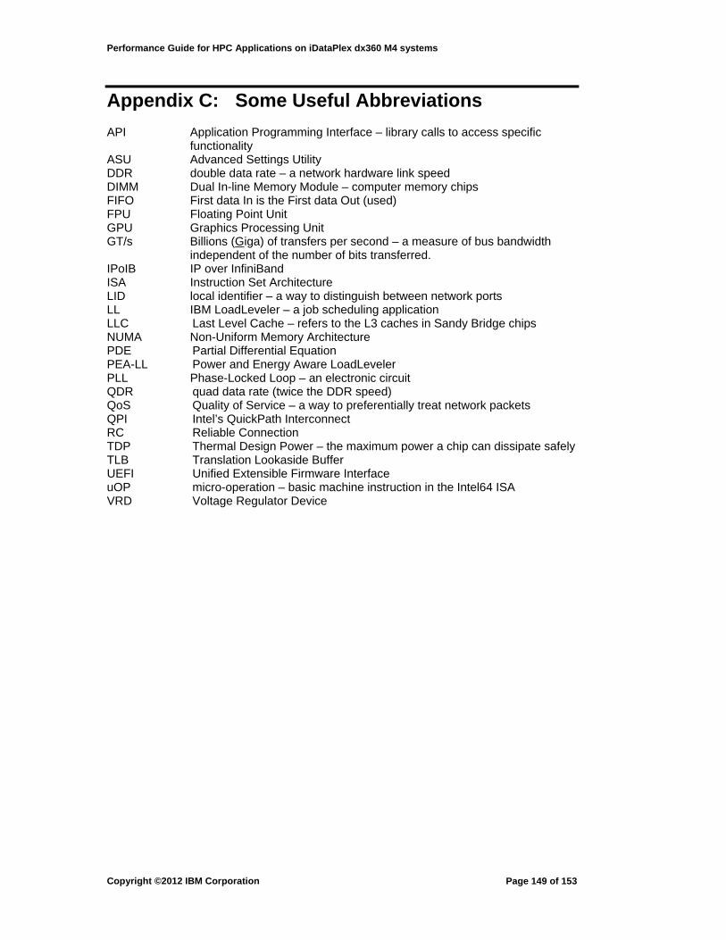
Performance Guide for HPC Applications on iDataPlex dx360 M4 systems
Appendix C: Some Useful Abbreviations
API Application Programming Interface – library calls to access specific functionality
ASU Advanced Settings Utility DDR double data rate – a network hardware link speed DIMM Dual In-line Memory Module – computer memory chips FIFO First data In is the First data Out (used) FPU Floating Point Unit GPU Graphics Processing Unit GT/s Billions (Giga) of transfers per second – a measure of bus bandwidth
independent of the number of bits transferred. IPoIB IP over InfiniBand ISA Instruction Set Architecture LID local identifier – a way to distinguish between network ports LL IBM LoadLeveler – a job scheduling application LLC Last Level Cache – refers to the L3 caches in Sandy Bridge chips NUMA Non-Uniform Memory Architecture PDE Partial Differential Equation PEA-LL Power and Energy Aware LoadLeveler PLL Phase-Locked Loop – an electronic circuit QDR quad data rate (twice the DDR speed) QoS Quality of Service – a way to preferentially treat network packets QPI Intel’s QuickPath Interconnect RC Reliable Connection TDP Thermal Design Power – the maximum power a chip can dissipate safely TLB Translation Lookaside Buffer UEFI Unified Extensible Firmware Interface uOP micro-operation – basic machine instruction in the Intel64 ISA VRD Voltage Regulator Device
Copyright ©2012 IBM Corporation
Page 149 of 153
Performance Guide for HPC Applications on iDataPlex dx360 M4 systems
Appendix D: Notices
© IBM Corporation 2010
IBM Corporation Marketing Communications, Systems Group Route 100, Somers, New York 10589 Produced in the United States of America March 2010, All Rights Reserved
This information was developed for products and services offered in the U.S.A.
IBM may not offer the products, services, or features discussed in this document in other countries. Consult your local IBM representative for information on the products and services currently available in your area. Any reference to an IBM product, program, or service is not intended to state or imply that only that IBM product, program, or service may be used. Any functionally equivalent product, program, or service that does not infringe any IBM intellectual property right may be used instead. However, it is the user's responsibility to evaluate and verify the operation of any non-IBM product, program, or service.
IBM may have patents or pending patent applications covering subject matter described in this document. The furnishing of this document does not give you any license to these patents. You can send license inquiries, in writing, to:
IBM Director of Licensing, IBM Corporation, North Castle Drive, Armonk, NY 10504-1785 U.S.A.
The following paragraph does not apply to the United Kingdom or any other country where such provisions are inconsistent with local law: INTERNATIONAL BUSINESS MACHINES CORPORATION PROVIDES THIS PUBLICATION "AS IS" WITHOUT WARRANTY OF ANY KIND, EITHER EXPRESS OR IMPLIED, INCLUDING, BUT NOT LIMITED TO, THE IMPLIED WARRANTIES OF NON-INFRINGEMENT, MERCHANTABILITY OR FITNESS FOR A PARTICULAR PURPOSE. Some states do not allow disclaimer of express or implied warranties in certain transactions, therefore, this statement may not apply to you.
This information could include technical inaccuracies or typographical errors. Changes are periodically made to the information herein; these changes will be incorporated in new editions of the publication. IBM may make improvements and/or changes in the product(s) and/or the program(s) described in this publication at any time without notice.
Any references in this information to non-IBM Web sites are provided for convenience only and do not in any manner serve as an endorsement of those Web sites. The materials at those Web sites are not part of the materials for this IBM product and use of those Web sites is at your own risk.
IBM may use or distribute any of the information you supply in any way it believes appropriate without incurring any obligation to you.
Information concerning non-IBM products was obtained from the suppliers of those products, their published announcements or other publicly available sources. IBM has not tested those products and cannot confirm the accuracy of performance, compatibility or any other claims related to non-IBM products. Questions on the capabilities of non-IBM products should be addressed to the suppliers of those products.
Copyright ©2012 IBM Corporation
Page 150 of 153

Performance Guide for HPC Applications on iDataPlex dx360 M4 systems
This information contains examples of data and reports used in daily business operations. To illustrate them as completely as possible, the examples include the names of individuals, companies, brands, and products. All of these names are fictitious and any similarity to the names and addresses used by an actual business enterprise is entirely coincidental.
COPYRIGHT LICENSE:
This information contains sample application programs in source language, which illustrate programming techniques on various operating platforms. You may copy, modify, and distribute these sample programs in any form without payment to IBM, for the purposes of developing, using, marketing or distributing application programs conforming to the application programming interface for the operating platform for which the sample programs are written. These examples have not been thoroughly tested under all conditions. IBM, therefore, cannot guarantee or imply reliability, serviceability, or function of these programs.
More details can be found at the IBM Power Systems home page6.
6 http://www.ibm.com/systems/p
Copyright ©2012 IBM Corporation
Page 151 of 153

Performance Guide for HPC Applications on iDataPlex dx360 M4 systems
Copyright ©2012 IBM Corporation
Page 152 of 153
Appendix E: Trademarks
IBM, the IBM logo, and ibm.com are trademarks or registered trademarks of International Business Machines Corporation in the United States, other countries, or both. These and other IBM trademarked terms are marked on their first occurrence in this information with the appropriate symbol (® or ™), indicating US registered or common law trademarks owned by IBM at the time this information was published. Such trademarks may also be registered or common law trademarks in other countries. A current list of IBM trademarks is available on the Web.
The following terms are trademarks of the International Business Machines Corporation in the United States, other countries, or both:
1350™ AIX 5L™ AIX® alphaWorks® Ascendant® BetaWorks™ BladeCenter® CICS® Cool Blue™ DB2® developerWorks® Domino® EnergyScale™ Enterprise Storage Server® Enterprise Workload Manager™ eServer™ Express Portfolio™ FlashCopy® GDPS® General Parallel File System™ Geographically Dispersed Parallel Sysplex™ Global Innovation Outlook™ GPFS™ HACMP™ HiperSockets™ HyperSwap™ i5/OS®
IBM Process Reference Model for IT™ IBM Systems Director Active Energy Manager™ IBM® iDataPlex® IntelliStation® Lotus Notes® Lotus® MQSeries® MVS™ Netfinity® Notes® OS/390® Parallel Sysplex® PartnerWorld® POWER™ POWER® POWER4™ POWER5™ POWER6™ POWER7™ PowerExecutive™ Power Systems™ PowerPC® PowerVM™ PR/SM™ pSeries® QuickPlace® RACF® Rational Summit®
Rational Unified Process® Rational® Redbooks® Redbooks (logo) ® RS/6000® RUP® S/390® Sametime® Summit Ascendant™ Summit® System i™ System p™ System Storage™ System x™ System z™ System z10™ System/360™ System/370™ Tivoli® TotalStorage® VM/ESA® VSE/ESA™ WebSphere® Workplace™ Workplace Messaging® X-Architecture® xSeries® z/OS® z/VM® z10™ zSeries®
The following terms are trademarks of other companies:
AMD™, AMD Opteron™, the AMD Arrow logo, and combinations thereof, are trademarks of Advanced Micro Devices, Inc.
InfiniBand™, and the InfiniBand design marks are trademarks and/or service marks of the InfiniBand Trade Association.
ITIL® is a registered trademark, and a registered community trademark of

Performance Guide for HPC Applications on iDataPlex dx360 M4 systems
the Office of Government Commerce, and is registered in the U.S. Patent and Trademark Office.
IT Infrastructure Library® is a registered trademark of the Central Computer and Telecommunications Agency which is now part of the Office of Government Commerce.
Novell®, SUSE®, the Novell logo, and the N logo are registered trademarks of Novell, Inc. in the United States and other countries.
Oracle®, JD Edwards®, PeopleSoft®, Siebel®, and TopLink® are registered trademarks of Oracle Corporation and/or its affiliates.
SAP NetWeaver®, SAP R/3®, SAP®, and SAP logos are trademarks or registered trademarks of SAP AG in Germany and in several other countries.
IQ™, J2EE™, Java™, JDBC™, Netra™, Solaris™, Sun™, and all Java-based trademarks are trademarks of Sun Microsystems, Inc. in the United States, other countries, or both.
Microsoft™, Windows™, Windows NT™, Outlook™, SQL Server™, Windows Server™, Windows™, and the Windows logo are trademarks of Microsoft Corporation in the United States, other countries, or both.
Intel Xeon™, Intel™, Itanium™, Intel logo, Intel Inside logo, Intel SpeedStep®, and the Intel Centrino logo are trademarks or registered trademarks of Intel Corporation or its subsidiaries in the United States, other countries, or both. A current list of Intel trademarks is available on the Web at http://www.intel.com/intel/legal/tmnouns2.htm.
QLogic™, the QLogic logo are the trademarks or registered trademarks of QLogic Corporation.
SilverStorm™ is a trademark of QLogic Corporation. SPEC® is a registered trademark of Standard Performance Evaluation
Corporation. SPEC MPI® is a registered trademark of Standard Performance Evaluation
Corporation. UNIX® is a registered trademark of The Open Group in the United States
and other countries. Linux™ is a trademark of Linus Torvalds in the United States, other
countries, or both.
Other company, product, or service names may be trademarks or service marks of others.
Copyright ©2012 IBM Corporation
Page 153 of 153