Int. J. of Critical Computer-Based Systems Vol. x, No. y, 2018 1

Performance Evaluation of Stochastic Real-TimeSystems with the SBIP Framework

Ayoub Nouri, Braham Lotfi Mediouni, MariusBozga, Jacques Combaz, Saddek BensalemUniv. Grenoble Alpes, CNRS, Grenoble INP*, VERIMAG38000 Grenoble, FranceE-mail: ayoub.nouri@univ-grenoble-alpes.fr* Institute of Engineering Univ. Grenoble Alpes

Axel Legay

INRIA, Rennes, France

Abstract: The SBIP framework consists of a stochastic real-time component-based modelling formalism and a statistical model checking engine. The formeris built as a stochastic extension of the real-time BIP formalism and enablesthe construction of stochastic real-time systems in a compositional way. Thestatistical engine implements a set of statistical algorithms for the quantitativeand qualitative assessment of probabilistic properties. The paper provides athorough introduction to the SBIP formalism and the associated verificationmethod. In a second part, it surveys several case studies about modellingand verification of real-life systems, including various network protocols andmultimedia applications.

Keywords: Stochastic systems, real-time, component-based, formal models,Generalised Semi-Markov Process, GSMP, BIP, Statistical Model Checking,SMC, performance evaluation.

1 Introduction

Stochastic models are of paramount importance in system design as they allow to captureuncertainties in systems behaviours and to account for variability induced by systemsenvironments. Such models offer, in addition, a mean for high-level reasoning and fordealing with complex systems in an abstract and quantitative fashion. This is highlyrecommended, especially during the first phases of the design process, where the numberof design choices is quite large. Modelling formalisms enabling to incorporate stochasticaspects are thus substantial.

In model-based design, it is recommended to rely on the same modelling formalismto handle both performance aspects, e.g., energy consumption, and functional behaviour,e.g., timing constraints. This enables to perform functional verification and performance

Copyright c� 2018 Inderscience Enterprises Ltd.

Preprint of the paper to appear in IJCCBS 2018 - International Journal of Critical Computer-Based Systems, Inderscience

2 A. Nouri et al.

evaluation in a consistent manner. Many real-life systems operate under stringent timingconstraints, e.g., real-time systems, which have the particularity to fail when missing wellspecified deadlines. Modelling formalisms that enable to capture both stochastic behaviourand timing constraints are essential for building faithful system models at a high-level ofabstraction, and to allow for their trustworthy assessment.

In this paper we present the SBIP framework which offers a stochastic real-timemodelling formalism and a statistical model checking (SMC) engine for quantitativeassessment of systems properties. The paper is an extended version of (Nouri et al., 2016a)that generalises the current stochastic modelling formalism (Nouri et al., 2015). We relyon the BIP (Behaviour, Interaction, Priority) framework (Basu et al., 2006) which allowsfor building heterogeneous and complex system models in a compositional fashion.

The stochastic real-time BIP formalism allows for building components as stochastictimed automata and to compose them by using multi-party interactions in order to build thefinal system. In these components, time evolves continuously and is modelled by using theclassical clock construct, introduced in timed automata (Alur and Dill, 1994). The proposedformalism enables for associating system events with timing constraints, e.g., an event onlyoccurs in a particular time interval. The latter can be further annotated with urgency tags,which specify their level of urgency. Furthermore, in order to express uncertainty regardingevents occurrences, it is possible to associate them with probability density functions.Hence, the precise moment of executing an event is scheduled according to that densityfunction.

In the SBIP modelling formalism, we consider two types of events, namely timed andstochastic. The former are associated with time constraints expressed as lower and upperbounds over clocks valuations, as in timed automata. These events are scheduled withrespect to a uniform or an exponential probability distribution as it is generally the casein several existing modelling formalisms. Although several probabilistic behaviours, e.g.,phase-type can be approximated by an exponential density, many real-life systems do notfollow such a probabilistic evolution. Restricting to these density functions is not a realisticassumption in our opinion. To overcome this lack, we introduce stochastic events, whichmay be scheduled with respect to arbitrary density functions, e.g., Normal, Poisson.

Enabling arbitrary probability density functions adds more complexity at the level ofthe mathematical construction induced by this model. An important reason for restrictingto exponential probability densities is their particularity of being memoryless, whichgenerally induces Markovian models. That is, the choice of the next system state onlydepends on the current one. Conversely, arbitrary density functions are not generallymemoryless and hence induce models taking into account the system history when movingto the next state. This leads to more general models, which in our case is a GeneralisedSemi-Markov Process (GSMP) (Kulkarni, 2011).

The SMC engine provided by the SBIP framework for stochastic models assessmentimplements well known statistical analysis algorithms, namely hypothesis testing (Younes,2005a) and probability estimation (Herault et al., 2004). Statistical model checking is anovel technique proposed as a trade-off between purely analytical verification techniquesand purely simulation-based methods. It requires, as in the classical model checkingsetting, to build an operational model of the stochastic system of interest and to provide aformal specification of the property to verify, generally using temporal logic. SMC exploresa sample of the stochastic model execution traces produced through simulation in orderto estimate the probability for the system to satisfy that property. This statistical approachis receiving an increasing attention and is being adopted in a wide range of application

Performance Evaluation of Stochastic Real-Time Systems with SBIP 3

domains such as in biology (David et al., 2015a), for the assessment of communicationprotocols (Basu et al., 2010a), multimedia applications (Raman et al., 2013), and avionics(Basu et al., 2010b).

Outline

The remainder of the paper is organised as follows. We discuss some related works inSection 2. Section 3 introduces the stochastic real-time BIP formalism and its simulationsemantics. Section 4 recalls some principles of statistical model checking and presents thetemporal logic used in the SBIP framework. Technical details about the structure of theSMC engine and its implementation are provided in Section 5. In Section 6, we survey themain case studies realised with the SBIP framework, and Section 7 concludes the paper.

2 Related Works

Several frameworks exist for modelling and analysing stochastic systems. In this paper,we restrict ourselves to discuss frameworks following a model checking-like procedure.Other methods related to the Queuing Theory and Network Calculus are beyond the scopeof this discussion. The considered frameworks generally differ in three points, namely,the expressiveness of their modelling formalism, the proposed analysis technique, and theproperties specification language they offer.

For instance, UPPAAL-SMC (David et al., 2015b; Jegourel et al., 2016) supportsStochastic Timed Automata (STAs), which are general models including Discrete andContinuous Time Markov Chains (DTMCs and CTMCs) for system modelling andWeighted Metric Temporal Logic (WMTL) for properties specification. In addition toDTMCs and CTMCs, PRISM (Kwiatkowska et al., 2011) allows to model MarkovDecision Processes (MDPs) and Probabilistic Timed Automata (PTAs). For propertiesspecification, it allows to use Probabilistic Computation Tree Logic (PCTL/PCTL*),Continuous Stochastic Logic (CSL), Linear-time Temporal Logic (LTL).

Other tools like Vesta (Sen et al., 2005) support, in addition to DTMCs and CTMCs,algebraic specification languages, i.e., PMaude (Kumar et al., 2003). PlasmaLab (Jegourelet al., 2012) is a modular statistical model checker that may be extended with externalsimulators and checkers. Its default configuration accepts discrete-time models specifiedin the PRISM modelling language and properties expressed in Probabilistic Bounded LTL(PBLTL). Ymer (Younes, 2005b) is one of the first frameworks to implement hypothesistesting algorithms. It considers GSMPs and CTMCs specified using a dialect of the PRISMmodelling language, and accepts both PCTL and CSL for requirements specification.

Our framework enables to model DTMCs, MDPs, and GSMPs. From a modellingperspective, it differs from PRISM as the latter considers PTAs – as the underlyingprobabilistic and timed model – which incorporate non-determinism and are generallyanalysable using numerical probabilistic model checking. From this point of view, theSBIP framework is closer to the UPPAAL-SMC and the Ymer frameworks. The latter allowsto model GSMPs, whereas we consider GSMPs with fixed-delays events as in (Brazdilet al., 2011). The UPPAAL-SMC provides a general stochastic timed semantics, i.e., STAs,however it is only limited to exponential and uniform density functions. Furthermore, thestochastic real-time BIP formalism allows for specifying urgency types on systems events.For properties specification, we rely on PBLTL for the moment, but we are planning toconsider more expressive logics such as WMTL.

4 A. Nouri et al.

3 Stochastic Real-Time BIP

The stochastic real-time BIP framework reconciles the real-time and stochastic extensionsof the BIP (Basu et al., 2006) framework. We recall that BIP has been introducedas a component-based framework where systems are obtained by composition ofuntimed atomic components with multi-party interactions, and coordinated using dynamicpriorities. RT-BIP (Abdellatif et al., 2013) extended BIP with real-time features and has(dense) real-time semantics based on timed automata concepts (Alur and Dill, 1994). S-BIP (Nouri et al., 2015) extended BIP with stochastic features and has (discrete) stochasticsemantics based on Markov chains.

In the newly proposed stochastic real-time BIP formalism, atomic components aredefined as timed automata extended with stochastic timing constraints. Composition isperformed as in BIP using multi-party interactions, that is, n-ary synchronisation amongcomponent actions. Priorities are not supported. The underlying semantics is defined as aGeneralised Semi-Markov Process (GSMP) where the interpretation of time is dense.

We start by defining the syntax of our model at the level of components and theircomposition. Then, we present the underlying stochastic simulation semantics.

3.1 Stochastic Real-Time Components

Stochastic real-time BIP components are essentially timed automata with urgencies,augmented with a new form of stochastic guards on clocks.

Let � be a set of density functions, that is, functions ⇢ : R�0 ! R�0 such thatR10 ⇢(t)dt = 1. We denote by dom(⇢) = {t | ⇢(t) 6= 0} the definition domain of ⇢, that is,

the set of values with a non-zero probability to occur. Let X be a set of clocks. We considertimed constraints (guards) ct and stochastic constraints (guards) cs on X , defined by:

ct ::= true | x ⇠ k | x� y ⇠ k | ct ^ c

tcs ::= x ./ ⇢

where x, y 2 X , k 2 R�0, ⇠ 2 {<,,=,�, >} and ⇢ 2 �. The meaning of timedconstraints is as usual. A stochastic constraint x ./ ⇢ holds iff x 2 dom(⇢). Nonetheless,in contrast to a timed constraint, it will enforce the specific stochastic distribution ⇢ on thevalues of x used to effectively satisfy the constraint, when used as a transition guard.

Definition 3.1: A stochastic real-time BIP component B is an extended timed automaton(L,X, P, T, `

0), where L is a finite set of locations, `0 2 L is the initial location, X isa finite set of clocks, P is a finite set of ports, and T is a finite set of transitions. Everytransition is of the form (`, p, gu, r, `0), denoted for more convenience as ` p gu r����! `

0, where`, `

0 2 L are the source and target locations, p 2 P is the triggering port, gu is a constraintg on X with an urgency u 2 {lazy , delayable}, and r ✓ X is the set of clocks to be reset.

The only noticeable difference between our definition of components and the timedautomata concerns the meaning to control the progress of time. Usually, timed automatarely on location invariants and/or specific types of locations (e.g., committed) to explicitlyconstrain the time progress. In our case, we rely on urgency types of transitions withthe following intuitive meaning. A delayable transition (abbreviated to d) prevents timeprogress at the upper time bound in g, i.e., time is enabled to progress in the source locationat most to that bound. In contrast, a lazy transition (abbreviated to l) does not have any

Performance Evaluation of Stochastic Real-Time Systems with SBIP 5

send

send

x := 0y := 0

[0 x 3]d

x := 0

[y ./W(�, k)]dfail

recover

x := 0

y := 0[3 x 4]ds0

s1

fail recover

x := 0

(a) Sender

z := 0

[1 z 3]lalarm

backrecv

z := 0

recv

r0

r1

alarm

z := 0

z := 0[1 z 2]d

back

(b) Receiver

Figure 1: Examples of stochastic real-time BIP components

impact on the time progress. Such a transition might not be fired at all in spite of the upperbound in g, i.e., time is enabled to progress indefinitely in the source location.

We call a port timed (resp. stochastic) if it appears on transitions with timed (resp.stochastic) constraints. We tacitly restrict to components where every port is either timedor stochastic, but not both. Moreover, we restrict to components that are time-portdeterministic, i.e., for a given source location `, time t and port p, only one target location`0 can be reached.

Example 3.1: The Sender component shown in Figure 1a has control locations s0, s1,ports send, fail, recover and clocks x, y. This component starts in s0, where it may senddata periodically in a specific time slot, defined through the timed constraint [0 x 3]d. The Sender component may fail when executing the stochastic port fail. The latteris associated with the guard [y ./W(�, k)]d, where W(�, k) is the Weibull probabilitydensity function with parameters �, k, and dom(W) ✓ R�0. This guard indicates thatthe component fails after some time scheduled according to W(�, k). After a failure, thecomponent recovers after some delay in [3 x 4]d, where it goes back to s0 and startssending again according to the same time constraints.

Example 3.2: Figure 1b shows a second component, namely the Receiver, which hascontrol locations r0, r1, ports recv, alarm, back and one clock z. The Receiver starts inlocation r0, where z is set to 0. From this initial location, the component either receivessome data through the self loop on r0 labelled by the timed port recv (recv is a timed portwith a guard set to true, i.e. it might be taken whenever the component is in r0), in whichcase z is reset to 0. Or, it may fire the timed transition labelled by the port alarm and movesto location r1, where the recv port is not enabled. One may think of this behaviour as adegraded mode, e.g., energy saving with an alarm. Note that the alarm port is associatedwith the timed constraint [1 z 3]l. Since the latter is lazy, the upper bound 3 couldbe ignored and the alarm transition might not be fired. From location r1, the componenttakes transition back after a delay specified through [1 z 2]d, to r0 and starts receivingagain. This transition is delayable so it must be taken at most at z = 2.

3.2 Composition of Stochastic Real-Time Components

Stochastic real-time components are composed using multi-party interactions. Aninteraction represents a strong synchronisation (i.e, rendez-vous) between transitionslocated in different components.

6 A. Nouri et al.

Given n stochastic real-time components (Bi)i=1,n, with disjoint sets of ports Pi, wedefine interactions a as subsets of ports from [n

i=1Pi, where:

• |a \ Pi| 1, for every i = 1, . . . , n, i.e., each component Bi participates in a by atmost one port Pi,

• a contains either one stochastic port and any number of timed ports with true guards,or any number of timed ports with arbitrary timed guards.

Consequently, an interaction is associated with a guard obtained by the conjunction ofthe guards of the participating ports. An interaction is called stochastic if it containsa stochastic port, and timed otherwise. The timed ports participating in stochasticinteractions are restricted to have precisely true guards. Intuitively, this ensures that theexecution time for such interactions is solely determined by the stochastic port. Whilethis restriction could be avoided at the price of slightly increasing the complexity of theforthcoming stochastic semantics, it has limited impact on the modelling capabilities –none of examples considered actually required other types of interaction beyond the twocategories above.

Definition 3.2: A stochastic real-time BIP system is defined as the composition�(B1, ..., Bn) of n components B1, ..., Bn with a set of interactions �.

Example 3.3: Consider the composition of the Sender and Receive componentsshown in Examples 3.1 and 3.2. The composition is operated through the interaction{send, recv}, which relates the send port of the Sender with the port recv of the Receiver.Figure 2 shows the two components and how they interact through the interaction {send,recv}. The nominal behaviour is when the Sender sends data to the Receiver throughinteraction {send,recv}. However, the former may fail when interaction {fail} takes place,which is potentially detected by the Receiver. The latter emits an alarm and switches into anon-receiving mode by executing interaction {alarm}. The two components resume theirnormal activity after some delay, through interactions {recover} and {back} respectively.

send

send

x := 0y := 0

[0 x 3]d

x := 0

fail

recover

x := 0

y := 0[3 x 4]d

z := 0

[1 z 3]lalarm

backrecv

z := 0

recv

Sender Receiver

s0

s1

r0

r1

fail recover alarm

z := 0

z := 0[1 z 2]d

back

x := 0

[y ./W(�, k)]d

Figure 2: Composition of two stochastic real-time BIP components

We further introduce some additional notations for defining the underlying operationalsemantics of a stochastic real-time BIP system. Let �(B1, ..., Bn) be a stochastic real-timeBIP system, where Bi=1,...,n = (Li, Xi, Pi, Ti, `

0i ).

Definition 3.3: We define states s as couples (~,~v), where ~= (`1, ..., `n) 2 L1 ⇥ ...⇥Ln is a global location, and ~v : [n

i=1Xi ! R�0 is a vector of clocks valuations.

Performance Evaluation of Stochastic Real-Time Systems with SBIP 7

We define d-succ((~,~v), a) as the discrete successor (partial) function that computesthe successor of a state (~,~v) when taking an interaction a. Let a = {pi}i2I suchthat I denotes the set of indices of the components participating in a. We defined-succ((~,~v), a) = (~0, ~v0) whenever:

• for every i 2 I, there exists an enabled transition `ipi g

uii ri�����! `

0i of Bi, that is:

– either gi is a timed constraint which is satisfied by the valuations of theconcerned clocks, i.e. ~v|Xi

|= gi, where ~v|Xiis the projection of the set of

clocks on the subset of clocks that are used in gi, or

– gi is a stochastic constraint x ./ ⇢ and ~v(x) 2 dom(⇢).

• all these transitions are simultaneously executed, that is, clocks are reset ~v0(x) = 0for all x 2 [i2Iri and stay unchanged ~v0(x) = ~v(x) otherwise.

• all the components that do not participate in a remain unchanged, that is, for everyj 62 I it holds `j = `

0j .

If no successor by interaction a exists at state (~,~v), we define d-succ((~,~v), a) = ?.We define t-succ((~,~v), t) as the time successor function that computes the successor of

a state (~,~v) for a time progress of t. It is a total function and is defined as t-succ((~,~v), t) =(~,~v + t). That is, it increases all the clocks in ~v by the amount of time t.

Finally, we define the function succ((~,~v), t, a) that computes the successor of a state(~,~v) when taking an interaction a after the time progress of t, which is a partial functiondefined as the composition succ((~,~v), t, a) = d-succ(t-succ((~,~v), t), a).

Definition 3.4: The operational semantics of a stochastic real-time BIP system is definedas the timed transition system T = (S, s0,�!S) where

• S is the set of states, and s0 is the initial state,

• �!S✓ S ⇥ (� [ R�0)⇥ S are transitions defined by the two rules

DISCRETEd-succ((~,~v), a) = (~0, ~v0)

(~,~v)a�!S (~0, ~v0)

TIME

t > 0,

8a delayable. (9t0. succ((~,~v), t0, a) 6= ?) ) (9t00 � t. succ((~,~v), t00, a) 6= ?)

(~,~v)t�!S (~,~v + t)

That is, according to the first rule, an enabled interaction can be fired at the current instantand the state updated. According to the second rule, time can progress as long as all enableddelayable interactions remain enabled. Note that a run of T is an infinite sequence � =

s0s1s2 · · · , such that siti,ai���!S si+1, for some ti 2 R�0 and ai 2 �, for all i � 0.

8 A. Nouri et al.

3.3 Stochastic Simulation Semantics

So far, we introduced the concepts of stochastic real-time BIP components and presentedtheir composition from an operational viewpoint. In this section, we show how this modelembraces a stochastic semantics in terms of a Generalised Semi-Markov Process (Kulkarni,2011).

GSMPs are stochastic process descriptions for a large class of discrete-event systems.A configuration of the GSMP is usually determined by a state and a set of active events,every one associated with a remaining lifetime, i.e. the amount of time during which itremains active. The choice of the event to be executed follows a race policy, which consistsof selecting the event having the smallest remaining lifetime. The execution itself occurswhen the remaining lifetime reaches 0 and triggers a state change and moreover, an updateof the set of active events. That is, several events could become inactive and thereforeremoved from the set, or could become active, and therefore added to the set. In the lattercase, the remaining lifetime is randomly chosen according to a (usually dense support)probability density function associated to the event.

The stochastic real-time BIP semantics follow the same intuition by consideringinteractions defined at composition as the GSMP events. Moreover, the associatedprobability density functions are obtained from the explicit density functions used instochastic guards of stochastic interactions or by some default densities (uniform orexponential) in the case of timed interactions. In the remainder of this section weintroduce the stochastic simulation algorithm and define precisely the different densitiesand sampling procedures.

3.3.1 Stochastic Simulation Algorithm

As for a GSMP, our simulation keeps track of the remaining lifetime of each interaction inorder to implement the race policy. To this end, we define configurations as follows.

Definition 3.5: We define a configuration z as a couple h(~,~v), ~wi, where (~,~v) is astate (as in Definition 3.3) and ~w : � ! R�0 [ {1} is a vector of remaining lifetime ofinteractions.

For an interaction a, the value ~w(a) represents the remaining lifetime at the currentglobal location ~ and a is said to be active if ~w(a) < 1. Moreover, we need to identifydependencies between interactions. As explained for the GSMPs, the execution of aninteraction might activate and/or deactivate other interactions. In the case of stochastic real-time BIP we consider that an interaction a has an impact on another interaction b, denotedby a . b, iff the guard of b changes due to the execution of a, that is, either because b hasdifferent timing constraints at the location(s) reached after executing a, or because a resetssome clocks explicitly involved in one of the constraints of b (before or after executinga). It is worth mentioning that, according to this definition, any interaction b activated ordeactivated due to the execution of a is considered to be impacted by a.

Algorithm 1 below presents the stochastic execution dynamics of a stochastic real-timeBIP system. The algorithm shows how to move from one configuration zk = h(~k,~vk), ~wkito another zk+1 = h(~k+1,~vk+1), ~wk+1i, starting from an initial configuration z0 =

h(~0,~v0), ~w0i. The first part of the algorithm computes this initial configuration as a vector~0 of the initial locations of components Bi of the system, a vector of initial valuations of

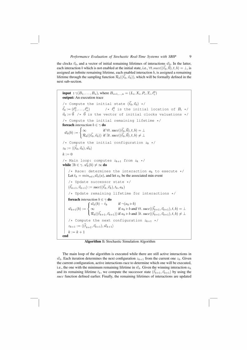
Performance Evaluation of Stochastic Real-Time Systems with SBIP 9

the clocks ~v0, and a vector of initial remaining lifetimes of interactions ~w0. In the latter,each interaction b which is not enabled at the initial state, i.e., 8t.succ((~0,~0), t, b) = ?, isassigned an infinite remaining lifetime, each enabled interaction b, is assigned a remaininglifetime through the sampling function Rb((~0,~v0)), which will be formally defined in thenext sub-section.

input : �(B1, . . . , Bn), where Bi=1,...,n = (Li, Xi, Pi, Ti, `0i )

output: An execution trace

/* Compute the initial state (~0,~v0) */~0 := (`01, . . . , `

0n) /* `

0i is the initial location of Bi */

~v0 := ~0 /* ~0 is the vector of initial clocks valuations */

/* Compute the initial remaining lifetime */foreach interaction b 2 � do

~w0(b) :=

(1 if 8t. succ((~0,~0), t, b) = ?Rb(( ~0,~v0)) if 9t. succ((~0,~0), t, b) 6= ?

/* Compute the initial configuration z0 */

z0 := h ~(`0,~v0), ~w0ik := 0

/* Main loop: computes zk+1 from zk */while 9b 2 �. ~wk(b) 6= 1 do

/* Race: determines the interaction ak to execute */Let tk = mina2� ~wk(a), and let ak be the associated min event

/* Update successor state */

(~k+1,~vk+1) := succ((~k,~vk), tk, ak)

/* Update remaining lifetime for interactions */

foreach interaction b 2 � do

~wk+1(b) :=

8<

:

~wk(b)� tk if ¬(ak . b)1 if ak . b and 8t. succ((~k+1,~vk+1), t, b) = ?Rb((~k+1,~vk+1)) if ak . b and 9t. succ((~k+1,~vk+1), t, b) 6= ?

/* Compute the next configuration zk+1 */

zk+1 := h~(`k+1,~vk+1), ~wk+1ik := k + 1

endAlgorithm 1: Stochastic Simulation Algorithm

The main loop of the algorithm is executed while there are still active interactions in~wk. Each iteration determines the next configuration zk+1 from the current one zk. Giventhe current configuration, active interactions race to determine which one will be executed,i.e., the one with the minimum remaining lifetime in ~wk. Given the winning interaction ak

and its remaining lifetime tk, we compute the successor state (~k+1,~vk+1) by using thesucc function defined earlier. Finally, the remaining lifetimes of interactions are updated

10 A. Nouri et al.

in this new state. Three cases can be distinguished for updating the vector of remaininglifetimes ~wk+1.

1. if interaction ak has no impact on b, then the remaining lifetime of b at (~k+1,~vk+1)

is its remaining lifetime at (~k,~vk) decreased by tk, i.e., the amount of time progress,

2. if interaction ak has an impact on b, and b is not active at (~k+1,~vk+1), then ~wk+1(b)is set to 1, that is, will not race in this new configuration,

3. if interaction ak has an impact on b, and b is active at (~k+1,~vk+1), then its remaininglifetime is sampled according to the function Rb((~k+1,~vk+1)).

Note that the enumerated settings include the case where new interactions are becomingactive at (~k+1,~vk+1). The reason is that any such interaction b is seen to be impacted byak as explained earlier.

It is worth explaining that the difference between interactions impacted by the executedinteraction ak and the non impacted ones, regarding the sampling operation is as follows.The former interactions involve ports of a shared component (i.e. involved in two or moreinteractions with different components), thus by executing ak the system state changes(potentially, the location of the shared component changes, some clocks are reset, etc.)and they need to be re-sampled as they are really seen as new interactions. For the latterinteractions, from their point of view nothing has changed but time has evolved, so we donot need to re-schedule them (by re-sampling) but just to update their remaining lifetimeaccordingly.

3.3.2 The Sampling Procedure

The sampling function Rb((~k+1,~vk+1)) used in Algorithm 1 computes the remaininglifetime for each interaction b when entering the state (~k+1,~vk+1) by taking interaction ak

from the state (~k,~vk). It depends on the type of interaction b, that is timed or stochastic,and delayable or lazy. For the sake of simplicity, we define the sampling procedure intwo phases: (1) in this subsection, we define the sampling procedure without detailing theunderlying probability density function, (2) in the next subsection, we will define how thedensity function is actually computed.

First let us consider the partitioning of interactions in a configuration h(~,~v), ~wi aseither fixed-delay interactions, denoted F or variable-delay interactions, denoted V . Fixed-delay interactions are induced by timed interactions having equality on their associatedtime constraints (also potentially by stochastic interactions following them), whereasvariable-delay interactions are timed or stochastic interactions with an interval of possibleremaining lifetime values.

F = {a 2 � | ~w(a) 6= 1, 9!t. succ((~,~v), t, a) 6= ?}V = {a 2 � | ~w(a) 6= 1} \ F

Based on this partitioning, the sampling function for an interaction b when entering a newstate (~,~v) is as follows.

Rb((~,~v)) =

8>><

>>:

t if b 2 F is delayable and enabled at tif X then t else 1 if b 2 F is lazy and enabled at t

F�1⇢b

(Y ) if b 2 V is delayableif X then F�1

⇢b(Y ) else 1 if b 2 V is lazy

Performance Evaluation of Stochastic Real-Time Systems with SBIP 11

where X ⇠ B( 12 ) is a random Bernoulli variable over {true, false}, i.e., true and falsehave a probability 1

2 , Y ⇠ U(0, 1) is a random variable with standard uniform distribution,and F�1

⇢bis the inverse cumulative distribution function (CDF) of the probability density

function ⇢b associated to b at (~,~v).For fixed-delay interactions (b 2 F), if b is delayable, the sampling function Rb((~,~v))

returns the single time value t that satisfies the guard gb. Whereas, if b is lazy, a discretechoice according to X is first performed to determine whether b will be considered andscheduled to t, or not considered and scheduled to 1.

The sampling function in the case of variable-delay interactions (b 2 V) is slightlymore involved since it requires choosing from an interval of time values. The sametreatment with respect to the urgency types of interactions is performed i.e., a discretechoice on X is used to consider a lazy interaction or not. The time value is obtainedby sampling according to the probability distribution ⇢b. Technically, this corresponds tocomputing the inverse CDF (F�1

⇢b) on a random value Y uniformly distributed in the interval

[0, 1]. The detailed definition of the probability density function ⇢b, in the case of timedand stochastic interactions, is given below.

3.3.3 Density Functions for Variable-delay Interactions

In this subsection, we define the density function ⇢b associated with a variable-delayinteraction b at a state (~,~v). We recall that such an interaction may be either timed orstochastic. For the former case, since no density function is explicitly specified on guards,the function ⇢b is obtained from a uniform or exponential density function. For the lattercase, the function ⇢b is obtained from the density function associated with the guard of b.

⇢b(t) =

8>>>>>>>><

>>>>>>>>:

1u� l

· 1[l t u] if b is timed with guard gb true on [l, u]

that is, ~vb + t |= gb iff t 2 [l, u]�e

��(t�l) · 1[l t] if b is timed with guard gb true on [l,1)that is, ~vb + t |= gb iff t 2 [l,1)

⇢(~vb(x) + t)Z 1

~vb(x)⇢(s)ds

if b is stochastic with guard [x ./ ⇢]

where 1[t 2 D] is the identity function, which gives 1 if t 2 D, and 0 otherwise.The first two cases correspond to timed interactions. We distinguish two situations in

this setting, (i) when interaction b is timed and has a right-bounded guard, i.e., u is finite,the sampling in the interval [l, u] is done uniformly, (ii) when the timed constraint is of theform [l,1), the sampling is done according to the exponential density function. In bothscenarios, the time t to sample must be within the interval specified by the time constraint.Stated differently, the current valuations of clocks in ~vb increased by the sampled time t

must satisfy the guard gb.Remark that for (i) and (ii), i.e., for timed interactions, the time constraint gb may

involve several clocks (potentially because of the composition, recall that an interactioninvolves several ports). Moreover, when entering a new state (~,~v), the concerned clocks~vb may have valuations different from 0. Hence, the computation of the final time boundsu, l in which the time t will be sampled, for b, either uniformly or exponentially is moreinvolved. Generally, given a guard gb of the form

Vi(li xi ui) and the valuations

12 A. Nouri et al.

~vb(xi), the bounds of the sampling interval of b are actually computed as l = max(li �~v(xi)) and u = min(ui � ~vb(xi)) as illustrated in the next example.

Example 3.4: The situation depicted in Figure 3 shows a global state of the system (~,~v),where the valuations of clocks x and y are respectively ~v(x) = 1 and ~v(y) = 2, and thetime constraint is [(2 x 6) ^ (2 y 5)]d. For the clock x, the remaining lifetimeinterval tx is computed as (2� 1) = 1 tx (6� 1) = 5. Similarly, for y, (2� 2) =0 ty (5� 2) = 3. Hence, the obtained sampling interval [l, u] is max(1, 0) t min(5, 3). Note that guards of the form x� y ⇠ k have the same interpretation since thedifference x� y is constant over time as both clocks evolve identically.

[(2 x 6) ^ (2 y 5)]d

(~, (~v(x) = 1,~v(y) = 2))

1 2 3 4 5 6

1

5

1 tx 5~v(x) = 1

3

0 ty 3

time

~v(y) = 2

1 t 3

Figure 3: Computation of upper and lower bounds in the case of timed interactions; l =max(1, 0) = 1 and u = min(5, 3) = 3, hence the sampling will be uniform in [1, 3].

The third case in the definition of ⇢b(t) concerns variable-delay interactions obtainedfrom a stochastic interaction b with a guard [x ./ ⇢]d. In this scenario, the sampling isdone in dom(⇢) according to a potentially shifted and normalised density function. Thistransformed function takes into account the case where the clock valuation of x, i.e., ~v(x)is not 0 when entering the state (~,~v). Below is a concrete illustration of the transformation.

Example 3.5: The transformation is illustrated in Figure 4, where ⇢(t) is a Normaldensity function and ~v(x) = 1. The function is first shifted to the current valuation of x,i.e., ⇢(1 + t). Since this shifted function is no longer a proper probability density function,i.e., its area is lower than 1, it is normalised, i.e., divided by

R11 ⇢(s)ds.

⇢(t)

Probability

t

~v(x)

Probability

t

e⇢(t) = ⇢(1+t)R 11 ⇢(s) ds

Shift and

Normalise

0 1 0

[x ./ ⇢]d

(~,~v(x) = 1)

Figure 4: Shifting and normalising a Normal density function in the case of stochasticinteractions

Performance Evaluation of Stochastic Real-Time Systems with SBIP 13

3.4 An Example of Stochastic Simulation

In Figure 5, we illustrate the stochastic semantics on Example 3.3 of the Sender-Receiver. We actually show a specific execution trace by sampling particulartime values in each configuration. In this figure, configurations are of the formh(si, rj), (~v(x),~v(y),~v(z)), (~w({send, recv}), ~w({fail}), ~w{recover}, ~w({alarm}),~w({back}))i. In each configuration, newly sampled remaining lifetimes are denoted bya box t , and updated remaining lifetimes are either 1 or underlined t according to thedefinition of the sampling function Rb . To make the example readable, we only show thediscrete transition, i.e. induced by the uniform choice over lazy interactions.

h(s0, r0), (0, 0, 0), ( 1.3 , 7.4 ,1, 2.8 ,1)ih(s0, r0), (0, 0, 0), ( 1.5 , 6 ,1,1,1)i

h(s0, r0), (0, 1.5, 0), ( 3 , 4.5,1,1,1)i

1.3, {send, recv}

h(s0, r0), (0, 4.5, 0), ( 2.3 , 1.5,1,1,1)i

12

1.5, {fail}

h(s1, r0), (0, 6, 1.5), (1,1, 3.5 ,1,1)i

h(s0, r0), (0, 1.3, 0), ( 2.6 , 6.1,1, 1.5,1)i

h(s1, r0), (0, 6, 1.5), (1,1, 3.5 , 1.5 ,1)i

h(s1, r1), (1.5, 7.5, 0), (1,1, 2,1, 1.3 )i

1.5, {alarm}

h(s1, r0), (2.8, 8.8, 0), (1,1, 0.7, 3 ,1)i

1.3, {back}

1.5, {send, recv}

3, {send, recv}

h(s1, r0), (2.8, 8.8, 0), (1,1, 0.7,1,1)i

0.7, {recover}

12

.5, {send, recv}

3.5, {recover}

0.7, {recover}

h(s0, r0), (0, 0, 0.7), ( .5 , 10 ,1, 2.3,1)i

Figure 5: Illustration of the stochastic simulation semantics on Example 3.3

In this example, there are two possible initial configurationscorresponding to the choice of considering the lazy interaction alarmh(s0, r0), (0, 0, 0), ( 1.3 , 7.4 ,1, 2.8 ,1)i or not h(s0, r0), (0, 0, 0), ( 1.5 , 6 ,1,1,1iat the beginning. Both configurations have the same global location and clocks valuation(s0, r0), (0, 0, 0), but differ in their sampling of the remaining lifetime of the initiallyracing interactions, namely {send, recv}, {fail} and {alarm}. In one case (left branch),we have (1.5, 6,1,1,1), i.e., alarm is scheduled at 1, while in the second case (rightbranch), (1.3, 7.4,1, 2.8,1), i.e., alarm is scheduled at 2.8. Note that the probabilityto start in one of these configurations corresponds to the probability to get the sampledremaining time values weighted by a half. For the sake of simplicity, we preferred todetail only one branch of the execution trace, i.e., the one on the left in Figure 5. Thecomplete execution trace shown in the example consists of the sequence of transitions1.5,{send,recv}����������! 3,{send,recv}���������! 1.5,{fail}������! 1.5,{alarm}��������! 1.3,{back}������! 0.7,{recover}���������! 0.5,{send,recv}����������!,

14 A. Nouri et al.

which corresponds to two send-receive operations, followed by a fail of the Sender, whichis detected by the Receiver that emits an alarm and moves to a degraded mode then getsback to its normal working mode, followed by a recover of the Sender, and finally anothersend-receive operation.

3.5 Additional Modelling Features

It is worth mentioning that the proposed model can be extended to allow for handling theusual cost/reward structures and data variables. For the sake of simplicity, we refrain fromproviding formal details for these additional modelling features and briefly provide someintuitions.

A cost/reward structure in this model can be obtained in a straightforward mannerby adding a data-structure in our simulation algorithm and associate it with states andinteractions. Since in our model we know how long the system remains in each state (as wekeep track of the remaining lifetimes of interactions), and which interactions are executed;we can, by specifying unit cost/reward for states and interactions, compute the global costfor each execution trace of the system. For instance, in the previous example, assume thatwe have this modelling feature and that we specified a cost of a fail to be 2, and the costof remaining in a failure mode as 1 per time unit. The total cost of the fragment of theexecution trace shown in Figure 5 will be 5.5. That is, 2 (the fail interaction cost) plus[(1.5 + 1.3 + 0.7)⇥ 1] (the total time spent by the Sender component in a failure mode,i.e., from executing interaction fail to executing interaction recover.

4 Statistical Model Checking

In this section we briefly recall the statistical model checking technique. We start by anoverview of the temporal logic used to specify systems properties and then we describe aset of well known SMC algorithms.

4.1 The PBLTL Temporal Logic

We first recap Bounded Linear-time Temporal Logic (BLTL) and then define itsprobabilistic extension. BLTL is an extension LTL (Baier and Katoen, 2008) wheretemporal operators can be bounded. The BLTL formulas that can be defined from a set ofatomic propositions P are the following.

• true , false , p, ¬p, for all p 2 P;

• �1 _ �2, �1 ^ �2;

• N�1, �1Ut�2.

where N is the next operator, Ut is the bounded until operator, �1 and �2 are BLTLformulas, and t is a positive integer. We also consider the usual temporal operators, namely,the bounded eventually Ft

� = trueUt�, and the bounded always Gt

� = ¬(trueUt(¬�)).The semantics of a BLTL formula is defined with respect to an execution trace ⇡ =

s0s1 . . . in the usual way (Clarke et al., 1999). Roughly speaking, an execution trace⇡ = s0s1 . . . satisfies N�1, which we denote ⇡ |= N�1, if state s1 of ⇡ satisfies �1. The

Performance Evaluation of Stochastic Real-Time Systems with SBIP 15

execution ⇡ satisfies �1Ut�2, which we denote ⇡ |= �1Ut

�2, iff there exists a state si withit that satisfies �2 and all the states in the prefix from s0 to si�1 satisfy �1.

In the SBIP framework, the properties specification language for stochastic systemsis a probabilistic variant of BLTL denoted PBLTL. More precisely, it consists of a BLTLformula preceded by a probabilistic operator P. Using this language, it is possible toformulate two types of queries on a given stochastic system as follows.

1. Qualitative queries : P�✓[�], where ✓ 2 [0, 1] is a probability threshold and � is aBLTL formula, also called path formula,

2. Quantitative queries : P=?[�], where � is a BLTL formula, also called path formula.

Note that it is possible through these queries to either determine if the probability forthe system to satisfy � is greater or equal to the threshold ✓ (using 1), or to ask for the actualprobability for the system to satisfy that property � (using 2). For instance, the PBLTLformula P=?[G1000(p)] stands for ”What is the probability that the atomic proposition p isalways satisfied?”. In this example, the path formula G1000(p) specifies that the length ofthe considered traces (i.e., the number of transitions to consider) is 1000.

4.2 The Main SMC Algorithms

We now present a model checking procedure to decide whether a given stochastic systemB satisfies a property �. Statistical model checking refers to a series of simulation-basedtechniques that can be used to answer two questions: (1) Qualitative: is the probability forB to satisfy � greater or equal to a certain threshold ✓? and (2) Quantitative: what is theprobability for B to satisfy �? Both questions can serve to decide a PBLTL property.

The main approaches (Herault et al., 2004; Younes, 2005a) proposed to answer thequalitative question are based on hypothesis testing. Let p be the probability of B |= �, todetermine whether p � ✓, we can test H : p � ✓ against K : p < ✓. A test-based solutiondoes not guarantee a correct result but it is possible to bound the probability of makingan error. The strength (↵,�) of a test is determined by two parameters, ↵ and �, suchthat the probability of accepting K (respectively, H) when H (respectively, K) holds isless or equal to ↵ (respectively, �). Since it is impossible to ensure a low probability forboth types of errors simultaneously (see Younes (2005a) for details), a solution is to use anindifference region [p1, p0] (with ✓ in [p1, p0]) and to test H0 : p� p0 against H1 : p p1.

Several hypothesis testing algorithms exist in the literature. Younes (2005a) proposeda logarithmic based algorithm that, given p0, p1,↵ and �, implements the Sequential RatioTesting Procedure (SPRT) (see Wald (1945) for details). When one has to test ✓�1 or✓�0, it is however better to use Single Sampling Plan (SSP) (see Bensalem et al. (2010);Herault et al. (2004); Younes (2005a) for details) that is another algorithm whose numberof simulations is pre-computed in advance. In general, this number is higher than the oneneeded by SPRT, but is known to be optimal for the above-mentioned values. More detailsabout hypothesis testing algorithms and a comparison between SSP and SPRT can be foundin (Bensalem et al., 2010).

In (Herault et al., 2004) Peyronnet et al. propose an estimation procedure(PESTIMATION) to compute the probability p for B to satisfy �. Given a precision �,Peyronnet’s procedure computes a value for p0 such that |p0 � p|� with confidence 1� ↵.The procedure is based on the Chernoff-Hoeffding bound (Hoeffding, 1963).

The efficiency of the above algorithms is characterised by the number of simulationsneeded to obtain an answer. This number may change from system to system and can only

16 A. Nouri et al.

be estimated (Younes, 2005a). However, some generalities are known. For the qualitativecase, it is known that, except for some situations, SPRT is always faster than SSP.PESTIMATION can also be used to solve the qualitative problem, but it is always slowerthan SSP (Younes, 2005a). If ✓ is unknown, then a good strategy is to estimate it usingPESTIMATION with a low confidence and then validate the result with SPRT and a strongconfidence.

It is worth mentioning that the statistical model checking technique is known towork for purely stochastic system model, i.e., non-determinism free. The stochastic real-time BIP modelling formalism guarantees that all non-determinism is resolved throughstochastic choices over interactions. SMC can be extended to handle non-deterministicmodels, e.g., MDPs, in which case it provides an interval of probabilities of satisfaction agiven property, by exploring all the possible schedules of the non-deterministic model.

5 The BIPSMC Engine

5.1 Architecture

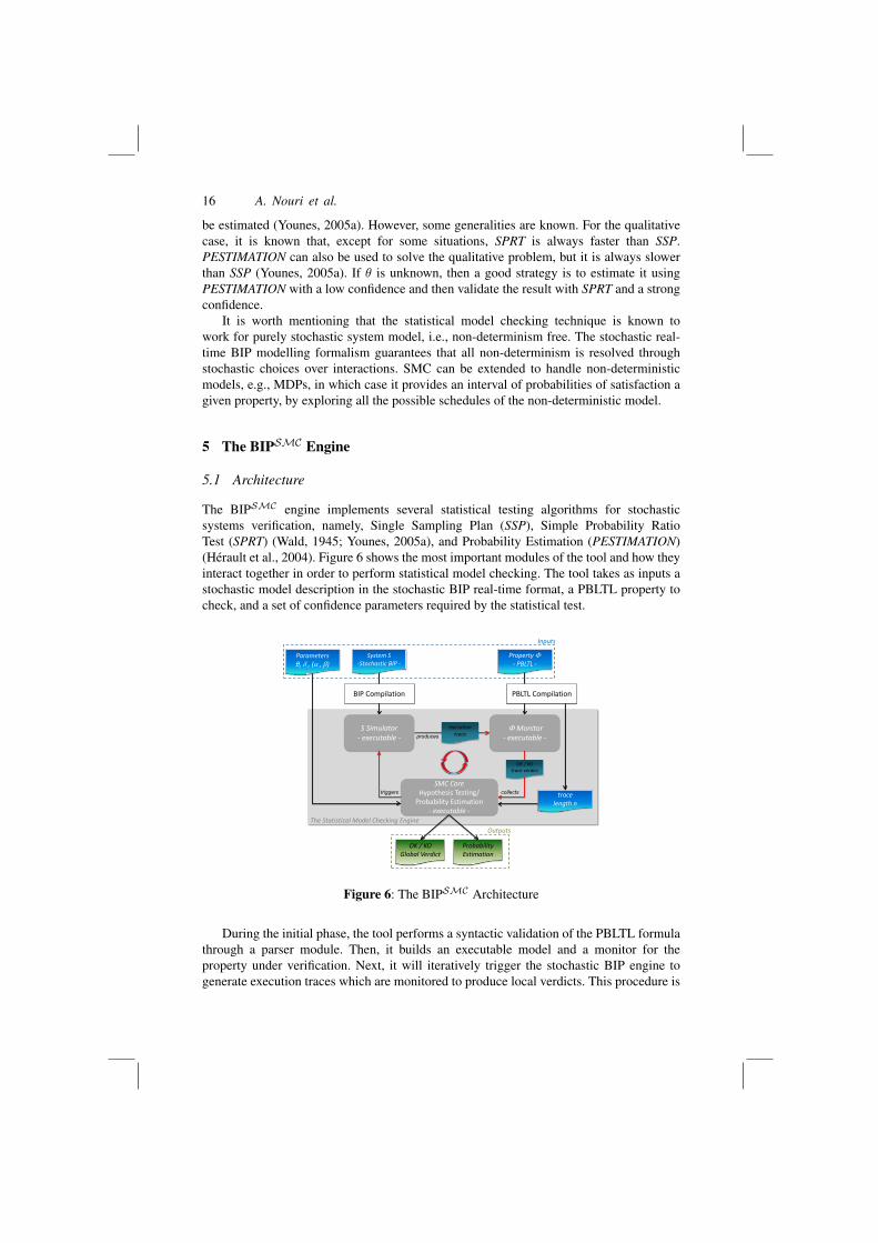
The BIPSMC engine implements several statistical testing algorithms for stochasticsystems verification, namely, Single Sampling Plan (SSP), Simple Probability RatioTest (SPRT) (Wald, 1945; Younes, 2005a), and Probability Estimation (PESTIMATION)(Herault et al., 2004). Figure 6 shows the most important modules of the tool and how theyinteract together in order to perform statistical model checking. The tool takes as inputs astochastic model description in the stochastic BIP real-time format, a PBLTL property tocheck, and a set of confidence parameters required by the statistical test.

S Simulator - executable -

BIP Compilation

Φ Monitor - executable -

SMC Core Hypothesis Testing/

Probability Estimation - executable -

System S -Stochastic BIP -

OK / KO trace verdict

OK / KO Global Verdict

execution trace

Property Φ - PBLTL -

PBLTL Compilation

Parameters ϑ, δ , (α , β)

triggers

produces

collects trace length n

Inputs

Probability Estimation

Outputs The Statistical Model Checking Engine

Figure 6: The BIPSMC Architecture

During the initial phase, the tool performs a syntactic validation of the PBLTL formulathrough a parser module. Then, it builds an executable model and a monitor for theproperty under verification. Next, it will iteratively trigger the stochastic BIP engine togenerate execution traces which are monitored to produce local verdicts. This procedure is

Performance Evaluation of Stochastic Real-Time Systems with SBIP 17

repeated until a global decision can be taken by the SMC core module (that implementsthe statistical algorithms). As our approach relies on SMC and since it considers boundedLTL properties, we are guaranteed that the procedure will eventually terminate.

It is worth mentioning that in our implementation, atomic propositions of PBLTLproperties are constructed from the system variables. For instance, the PBLTL formulaP=?[G1000(abs(Master.tm� Slave.ts) 160)] stands for ”What is the probability thatthe difference between master variable tm and slave variable ts is always under the bound160 ?”. In this example, Master.tm and Slave.ts are systems variables pertaining tocomponents Master and Slave respectively. Note that properties specification languageoffers the possibility to use built-in mathematical functions. In the example above, theabs() function is used to compute the absolute value of (Master.tm� Slave.ts).

5.2 Technical Details and Availability

BIPSMC is fully developed in the Java programming language. It uses JEP 2.4.1library (http://www.singularsys.com/jep/index.html, under GPL license)for parsing and evaluating mathematical expressions, and ANTLR 3.2 (http://www.antlr.org/) for PBLTL properties parsing and monitoring. At this stage,BIPSMC only runs on GNU/Linux operating systems as it relies on the BIP simulationengine. The current release of the tool has been enriched with a graphical userinterface for more convenience (see Figure 7 for a screen shot). The current versionalso includes support for the BIP2 language (http://www-verimag.imag.fr/New-BIP-tools.html) while still ensuring compatibility with the previous version.The model checker is available for download from http://www-verimag.imag.fr/Statistical-Model-Checking.html, where additional information (videotutorial) on how to install it and to use it can also be found.

Figure 7: Screen shot of the BIPSMC graphical user interface.

18 A. Nouri et al.

6 Case Studies

While still at the prototype level, the SBIP framework has been used to evaluate severallarge-scale systems that cover different application domains. In this section we surveysome of these studies and discuss their results. The first two studies consider the modellingand assessment of multimedia applications, while the three remaining present networkingapplication and protocols. For the sake of conciseness, we show for some of them howthe underlying models are built in the proposed stochastic formalism. We also refer to theoriginal publications for further details such as the verification times.

6.1 An MPEG2 Decoder Subsystem

In this study, the SBIP framework is used to check QoS properties of an MPEG2 decodersubsystem part of a video streaming application (Raman et al., 2013). This work is aboutfinding a good trade-off, when designing the multimedia system, between the requiredsizes of the system buffers and the quality of delivered videos. It is known in the literaturethat an acceptable amount of quality degradation – defined as less than two consecutiveframes within one second – can be tolerated in order to reduce buffers sizes (Raman et al.,2013). The study will consist to assess this requirement.

write push pop read write push pop read

Player(Rate, Delay)

PlayoutBuffer(Size)

Processor(Frequency)

InputBuffer(Size)

Generator(BitRate)

Figure 8: The abstract MPEG2 decoder model.

The model in Figure 8 is used to represent the considered MPEG2 subsystem. It showsits different parts, namely, the Generator, the Input and the Playout buffers, the Processor,which decodes the input videos macro-blocks, and the Player device. In this study, qualitydegradation is seen as a buffer underflow, which occurs whenever the Player device failsto read sufficient macro-blocks from the Playout buffer. Note that the amount of underflowis impacted by the parameter Delay of the Player, that represents the delay after which itstarts playing the decoded video frames.

l3l0l0 l1

l1l2l2

gen frm

ft = ‘B‘

x++

gen frm

ft = ‘P ‘

x++

gen frm

ft = ‘B‘

x++

gen frm [x == 12]ft = ‘I‘

x++

mbt = ft

gen mb

[x < 330]

[x == 330]x = 0

read

gen frm

[x 2 [3, 6, 9]]

x++;

gen frmft

gen mbmbt

readft

read

write write

l0

write

mbs = fmbt()

readmbt mbs

l1[y ./ ⇢mbt]d

y := 0

y := 0

x = 0 x = 0

x++

Figure 9: The Generator compound component. The probability density function ⇢mbt

captures the arrival delays of videos macro-blocks.

Figure 9 shows the detailed behaviour of the Generator component. The latter modelsthe arrival of encoded videos macro-blocks to the MPEG2 decoder subsystem in a

Performance Evaluation of Stochastic Real-Time Systems with SBIP 19

stochastic fashion. This component is made of three sub-components operating as follows.The first component (left) generates frames following the MPEG2 GOP pattern (Ramanet al., 2013). Each frame is then decomposed, in the second component, into 330 macro-blocks, which are finally transmitted to the third component that models the macro-blocksstochastic arrival time to the input buffer with respect to ⇢mtb.

Some of the obtained results in this study, using the SMC technique, are illustratedin Figure 10. The latter shows three different curves, each corresponding to a differentanalysed video, namely cact.m2v, mobile.m2v, and tennis.m2v, having the sameresolution of 352⇥ 240. Each curve shows the evolution of the probability that the qualitydegradation is always less than two consecutive frames within one second, for differentvalues of the Delay parameter. This result helps to determine the right Delay parameterto use. Note that for these experiments, the BIPSMC engine required about 44 to 7145traces each time and spent around 6 to 8 seconds in average to check the property with aconfidence bound of 10�2.

0 100 200 300 400 500

0.0

0.2

0.4

0.6

0.8

1.0

Initial Playout Delay (ms)

P(lo

ss <

2 c

onse

cutiv

e fra

mes

)

cact.m2vmobile.m2vtennis.m2v

Figure 10: Probability of avoiding quality degradation in three different videos forincreasing values of the Initial Playout Delay.

6.2 Image Recognition on Many-cores

In this case study, the SBIP framework is used as part of the design of an embedded systemconsisting of the HMAX image recognition application deployed on the STHORM many-core architecture (Nouri et al., 2014, 2016b).

The HMAX model algorithm (Mutch and Lowe, 2008) is a hierarchical computationalmodel of object recognition – in input images – which attempts to mimic the rapid objectrecognition of human brain. The case study focuses on the first layer of the HMAX modelalgorithm, denoted S1 in Figure 11, as it is the most computationally intensive.

The goal of the study is to explore several design parameters with respect to timingconstraints, that is, the overall execution time, and the time to process single lines ofan input image. More precisely, the analysis consists of probabilistically quantifying therequirement that the overall execution time is always lower than a given bound, denoted�, and that the variability in the processing time of successive lines is always boundedby . To this extent, the above requirements were respectively specified in BLTL as �1 =

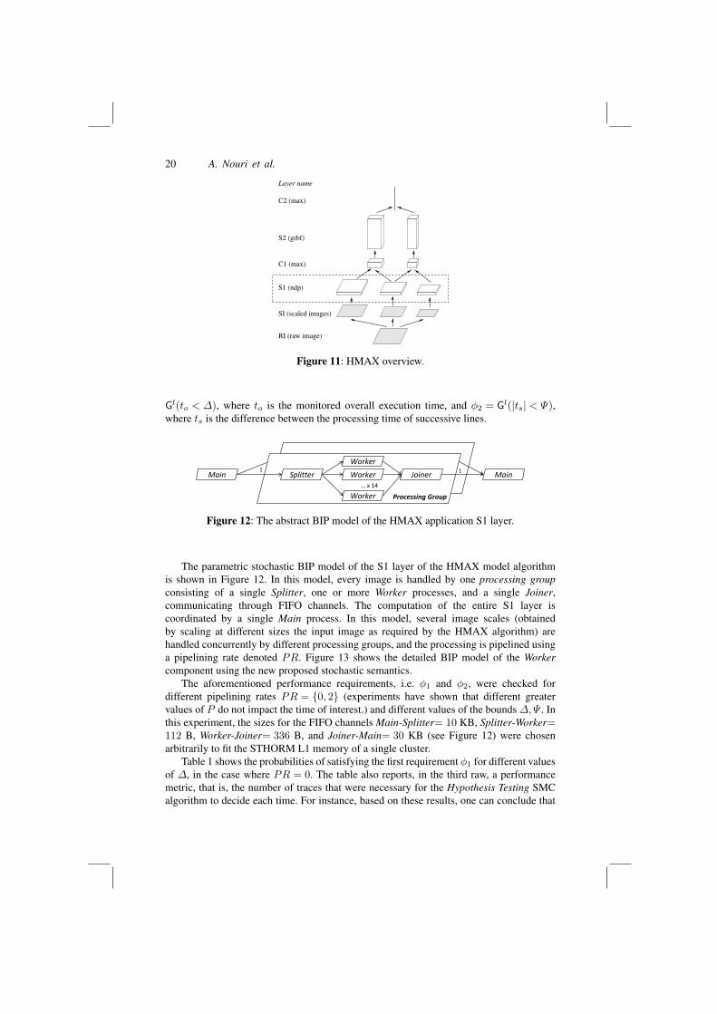
20 A. Nouri et al.

C2 (max)

S2 (grbf)

C1 (max)

S1 (ndp)

SI (scaled images)

Layer name

RI (raw image)

Figure 11: HMAX overview.

Gl(to < �), where to is the monitored overall execution time, and �2 = Gl(|ts| < ),where ts is the difference between the processing time of successive lines.

Worker

Worker

Worker

… x 14

Splitter Joiner Main Main

Processing Group

… …

Figure 12: The abstract BIP model of the HMAX application S1 layer.

The parametric stochastic BIP model of the S1 layer of the HMAX model algorithmis shown in Figure 12. In this model, every image is handled by one processing groupconsisting of a single Splitter, one or more Worker processes, and a single Joiner,communicating through FIFO channels. The computation of the entire S1 layer iscoordinated by a single Main process. In this model, several image scales (obtainedby scaling at different sizes the input image as required by the HMAX algorithm) arehandled concurrently by different processing groups, and the processing is pipelined usinga pipelining rate denoted PR. Figure 13 shows the detailed BIP model of the Workercomponent using the new proposed stochastic semantics.

The aforementioned performance requirements, i.e. �1 and �2, were checked fordifferent pipelining rates PR = {0, 2} (experiments have shown that different greatervalues of P do not impact the time of interest.) and different values of the bounds �, . Inthis experiment, the sizes for the FIFO channels Main-Splitter= 10 KB, Splitter-Worker=112 B, Worker-Joiner= 336 B, and Joiner-Main= 30 KB (see Figure 12) were chosenarbitrarily to fit the STHORM L1 memory of a single cluster.

Table 1 shows the probabilities of satisfying the first requirement �1 for different valuesof �, in the case where PR = 0. The table also reports, in the third raw, a performancemetric, that is, the number of traces that were necessary for the Hypothesis Testing SMCalgorithm to decide each time. For instance, based on these results, one can conclude that

Performance Evaluation of Stochastic Real-Time Systems with SBIP 21

[steps != 0]

end_write_databegin_write_data

end_read_databegin_read_data

read(data_fifo_in, &data)

begin_write_data

write(data_fifo_out, data)

compute_filter(&data)

steps−−

end_write_data

end_read_data[status == _exec] begin_read_data

[steps == 0]status = _cfg

[status == _cfg]

read_conf

read(conf_fifo, &config)

read_conf

config

status = _exec

steps = config.steps

data

data

status = _cfg

`2

`7

`3`0

[x ./ ⇢w]d

[x ./ ⇢c]d

x := 0

x := 0

x := 0x := 0

[x ./ ⇢r]d

`1 `5

`4

`6

Figure 13: The stochastic BIP model of the Worker component, ⇢r, ⇢c, ⇢w are respectivelythe probability density functions of the time to read, to compute, and to write data.

Table 1 Probabilities to satisfy �1 for different bounds � and a fixed pipelining rate PR = 0.

�(ms) 572.75 572.8 572.83 572.85 572.89 572.91 572.95P(�1) 0 0.28 0.57 0.75 0.98 0.99 1

Nb. of traces 66 1513 1110 488 171 89 66

the expected overall execution time for processing one image scale is bounded by � =572.91ms with probability equal to 0.99.

2090 2100 2110 2120 2130 2140

0.0

0.2

0.4

0.6

0.8

1.0

� (µs)

Prob

abilit

y

(a) PR = 0

2270 2280 2290 2300 2310 2320

0.0

0.2

0.4

0.6

0.8

1.0

� (µs)

Prob

abilit

y

(b) PR = 2

Figure 14: Probability to satisfy �2 for PR 2 {0, 2}.

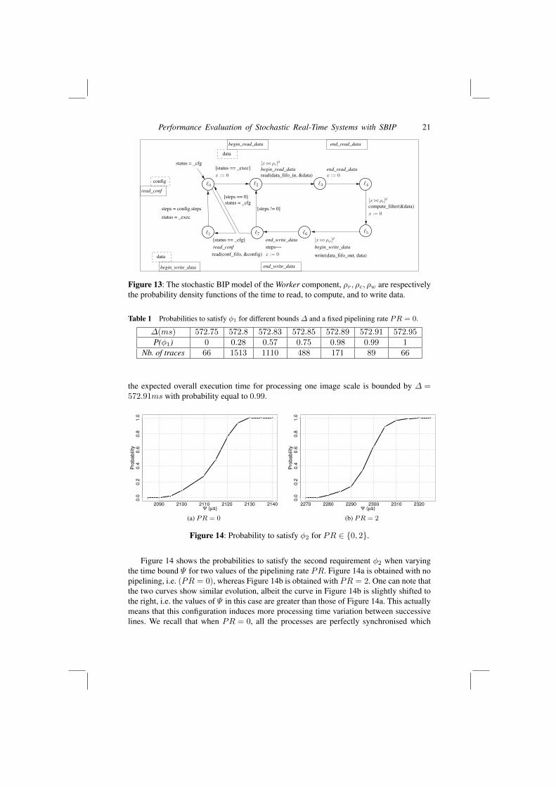
Figure 14 shows the probabilities to satisfy the second requirement �2 when varyingthe time bound for two values of the pipelining rate PR. Figure 14a is obtained with nopipelining, i.e. (PR = 0), whereas Figure 14b is obtained with PR = 2. One can note thatthe two curves show similar evolution, albeit the curve in Figure 14b is slightly shifted tothe right, i.e. the values of in this case are greater than those of Figure 14a. This actuallymeans that this configuration induces more processing time variation between successivelines. We recall that when PR = 0, all the processes are perfectly synchronised which

22 A. Nouri et al.

yields small variation over successive lines processing time. Using PR > 0 however leadsto greater variation since it somehow alters this synchronisation. Concretely, Figure 14shows that without pipelining, we obtain smaller expected time variation (of processingsuccessive lines). For instance when PR = 0, = 2128µs with probability 0.99, whereasfor PR = 2, = 2315µs with the same probability. One may conclude that, in this casestudy, a pipeline implementation will not help enhancing the system throughput.

6.3 The Precision Time Protocol – IEEE 1588

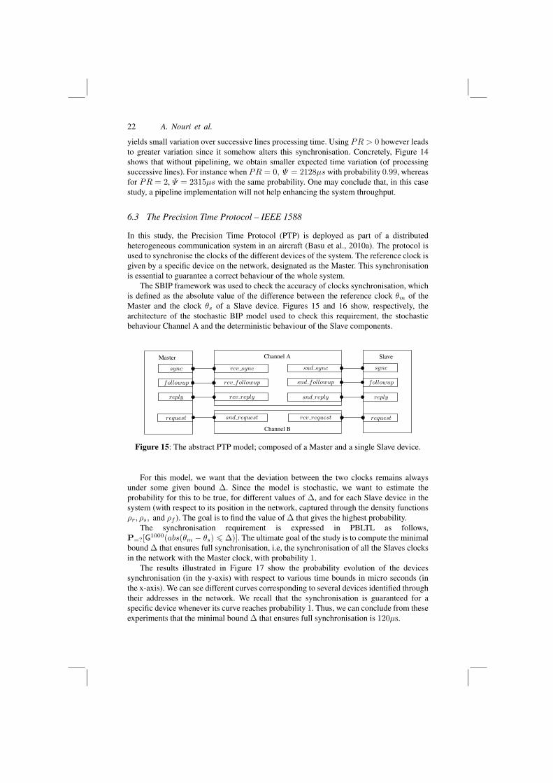
In this study, the Precision Time Protocol (PTP) is deployed as part of a distributedheterogeneous communication system in an aircraft (Basu et al., 2010a). The protocol isused to synchronise the clocks of the different devices of the system. The reference clock isgiven by a specific device on the network, designated as the Master. This synchronisationis essential to guarantee a correct behaviour of the whole system.

The SBIP framework was used to check the accuracy of clocks synchronisation, whichis defined as the absolute value of the difference between the reference clock ✓m of theMaster and the clock ✓s of a Slave device. Figures 15 and 16 show, respectively, thearchitecture of the stochastic BIP model used to check this requirement, the stochasticbehaviour Channel A and the deterministic behaviour of the Slave components.

sync

Channel AMaster

followup

reply

request

rcv followup

rcv sync

rcv reply

snd followup

snd sync

snd reply

sync

Slave

followup

reply

request

Channel B

snd request rcv request

Figure 15: The abstract PTP model; composed of a Master and a single Slave device.

For this model, we want that the deviation between the two clocks remains alwaysunder some given bound �. Since the model is stochastic, we want to estimate theprobability for this to be true, for different values of �, and for each Slave device in thesystem (with respect to its position in the network, captured through the density functions⇢r, ⇢s, and ⇢f ). The goal is to find the value of � that gives the highest probability.

The synchronisation requirement is expressed in PBLTL as follows,P=?[G1000(abs(✓m � ✓s) 6 �)]. The ultimate goal of the study is to compute the minimalbound � that ensures full synchronisation, i.e, the synchronisation of all the Slaves clocksin the network with the Master clock, with probability 1.

The results illustrated in Figure 17 show the probability evolution of the devicessynchronisation (in the y-axis) with respect to various time bounds in micro seconds (inthe x-axis). We can see different curves corresponding to several devices identified throughtheir addresses in the network. We recall that the synchronisation is guaranteed for aspecific device whenever its curve reaches probability 1. Thus, we can conclude from theseexperiments that the minimal bound � that ensures full synchronisation is 120µs.

Performance Evaluation of Stochastic Real-Time Systems with SBIP 23

t1

t1

t4

rcv sync

xs := 0

rcv followup

xf := 0 [xs ./ ⇢s]dsnd sync

rcv followup

xf := 0

[xf ./ ⇢f ]dsnd followup

rcv reply

xr := 0

snd reply

t1

t1

t4

[xs ./ ⇢s]dsnd sync

[xr ./ ⇢r]d

l4

l0

l1

l2 l3

l5

snd sync

snd followup

snd replyrcv reply

rcv followup

rcv sync

(a) Channel A

followup

sync

t2 := �s

reply

o := (t2 + t3 � t1 � t4)/2

�s := �s � o

request

t3 := �s

t1

t1

t4

t4

l0

l1

l2

l3

sync

followup

reply

request

(b) Slave

Figure 16: A detailed view of the Channel A and the Slave Components

Bound0 20 40 60 80 100 120 140

Probability

0.1

0.2

0.3

0.4

0.5

0.6

0.7

0.8

0.9

1

(0,0)(1,0)(2,0)(2,3)(3,0)

Figure 17: PTP accuracy analysis results

6.4 Wireless Sensor Network

The SBIP framework has been used to verify several networked systems based on differenttechnologies, CAN-based (Lekidis et al., 2013), Sensor Network using Wi-Fi (Lekidiset al., 2015a), and IoT applications (Lekidis et al., 2015b). We briefly present its utilisationfor the modelling and analysis of a Wireless Sensor Network (WSN) case study.

This case study concerns an audio streaming application over a Wi-Fi network, whereseveral nodes equipped with microphones produce different audio streams, which aretransmitted to a base station equipped with a speaker to play the received audio. The goalof the study is to ensure the synchronisation between the different nodes of the network inorder to guarantee a consistent audio output. To this extent, a Phase Locked Loop (PLL)

24 A. Nouri et al.

synchronisation protocol is deployed as part of the application nodes. The protocol worksas follows. The base station broadcasts periodically a frame containing the hardware clockvalue to all the nodes through the network. Each node applies the PLL synchronisationmechanism, to construct a software clock, that serves to keep its local clock synchronisedwith the received one.

TICK

READ

speaker

SEND RECV

RECV

REQ REQ

RECV

Sbuffer

TICK

SEND RECV

CLK_RECV

LOCAL_CLK

CLK_REQ

CLK_RES

Slavemicro

LOCAL_CLK

AUDIO_SEND

CLK_REQ

CLK_RES

Mbuffer WiFiMclock

GET_CLK

Sclock

CLK_SEND

TICK synchroTICK

Master

PLL

Figure 18: SBIP model of the Wireless Sensor Network

A BIP model of this application, following a Master-Slave architecture, was built. Asshown in Figure 18, it consists of a Master component that represents the base station,a Slave component that represents a particular node in the network, a Wi-Fi componentmodelling the Wi-Fi communication channel, and two buffer components, namely Mbufferand Sbuffer. In this model, the period of broadcasting the hardware clock is fixed toT = 5s. Each node uses its local clock to time-stamp the produced audio frames, so thatthe base station is able to reproduce the received audio frames in the correct order. Thesynchronisation accuracy is defined as the difference between the hardware clock and thecomputed software clock in each node and is required to be lower or equal to 1µs.

The WSN application implementation was generated from the functional modelshown in Figure 18 and deployed over three UDOO (http://www.udoo.org/features/) nodes, each consisting of a computational core, a Wi-Fi card, and asound card. The wireless network is supported by the Snowball SDK (http://www.calao-systems.com/articles.php?pg=6186), which is used as an AccessPoint (AP). This implementation is used to learn the probability distributions thatcharacterise the communication delays in order to build the stochastic BIP model used laterfor analysis.

Two sets of experiments were conducted, focusing on equally important requirementsfor the design of multimedia sensor networks. The first concerns the utilisation of thebuffer components regarding the audio streaming capturing and reproduction in the system.The second focuses on the clock synchronisation accuracy. For the second requirement,the difference between the Master clock ✓m and the software clock, computed in everySlave ✓s, without the impact of the audio capturing and reproduction, is observed. Bothrequirements were described as probabilistic temporal properties, using PBLTL. Theobtained results are presented hereafter.

We evaluated the property of avoiding buffers overflow (respectively underflow)by considering the following property �1 = Gl(SSbuffer < MAX) (respectively �2 =Gl(SMbuffer > 0)), where SSbuffer (respectively SMbuffer) indicates the size of theSlave (respectively the Master) buffer, and MAX is a positive integer value whichrepresents the capacity of the buffer. The left curve in Figure 19 shows the probability of

Performance Evaluation of Stochastic Real-Time Systems with SBIP 25

●●●●●●●●●●●●●●●●●●●●●●●●●●●●●●●●●●●●●●●●●●●●●●●●●●●●●●●●●●●●●●●●●●●●●●●●●●●●●●●●●●●●●●●●●●●●●●●●●●●●●●●●●●●●●●●●●●●●●●●●●●●●●●●●●●●●●●●●●●●●●●●●●●●●●●●●●●●●●●●●●●●●●●●●●●●●●●●●●●●●●●●●●●●●●●●●●●●●●●●●●●●●●●●●●●●●●●●●●●●●●●●●●●●●●

●●●●●●●●●●●●●●●●●●●●●●●●●●●●●●●●●●●●●●●●●●●●●●●●●●●●●●●●●●●●●●●●●●●●●●●●●●●●●●●●

●●●●●●●●●●●●●●●●●●●●●●●●●●●●●●●●●●●●●●●●●●●●●●●●●●

●●●●●●●●●●●●●●●●●●●●●●●●●●●●●●●●●●●●●●●●●●●●●●●●●●●●●●●●●●●●●●●●●●●●●●●●●●●●●●●●●●●●●●●●●●●●●●●●●●●●●●●●●●●●●●●●●●●●●●●●●●●●●●●●●●●●●●●●●●●●●●●●●●●●●●●●●●●●●●●●●●●●●●●●●●●●●●●●●●●●●●●●●●●●●●●●●●●●●●●●●●●●●●●●●●●●●●●●●●●●●●●●●●●●●●●●●●●●●●●●●●●●●●●●●●●●●●●●●●●●●●●●●●●●●●●●●●●●●●●●●●●●●●●●●●●●●●●●●●●●●●●●●●●●●●●●●●●●●●●●●●●●●●●●●●●●●●●●●●●●●●●●●●●●●●●●●●●●●●●●●●●●●●●●●●●●●●●●●●●●●●●●●●●●●●●●●●●●●●●●●●●●●●●●●●●●●●●●●●●●●●●●●●●●●●●●●●●●●●●●●●●●●●●●●●●●●●●●●●●●●●●●●●●●●●●●●●●●●●●●●●●●●●●●●●●●●●●●●●●●●●●●●●●●●●●●●●●●●●●●●●●●●●●●●●●●●●●●●●●●●●●●●●●●●●●●●●●●●●●●●●●●●●●●●●●●●●●●●●●●●●●●●●●●●●●●●●●●●●●●●●●●●●●●●●●●●●●●●●●●●●●●●●●●●●●●●●●●●●●●●

0 100 200 300 400 500 600 700 800 900 1000

020

4060

80100

size(Sbuffer)

Probability(%)

(a) P (�1) when increasing the Sbuffer size

●●●●●●●●●●●●●●●●●●●●●●●●●●●●●●●●●●●●●●●●●●●●●●●●●●●●●●●●●●●●●●●●●●●●●●●●●●●●●●●●●●●●●●●●●●●●●●●●●●●●●●●●●●●●●●●●●●●●●●●●●●●●●●●●●●●●●●●●●●●●●●●●●●●●●●●●●●●●●●●●●●●●●●●●●●●●●●●●●●●●●●●●●●●●●●●●●●●●●●●●●●●●●●●●●●●●●●●●●●●●●●●●●●●●●

●●●●●●●●●●●●●●●●●●●●●●●●●●●●●●●●●●●●●●●●●●●●●●●●●●●●●●●●●●●●●●●●●●●●●●●●●●●●●●●●●●●●●●●●●●●●●●●●●●●●●●●●●●●●●●●●●●●●●●●●●●●●●●●●●●●●●●●●●●●●●●●●●●●●●●●●●●●●●●●●●●●●●●●●●●●●●●●●●●●●●●●●●●●●●●●●●●●●●●●●●●●●●●●●●●●●●●●●●●●●●●●●●●●●●●●●●●●●●●●●●●●●●●●●●●●●●●●●●●●●●●●●●●●●●●●●●●●●●●●●●●●●●●●●●●●●●●●●●●●●●●●●●●●●●●●●●●●●●●●●●●●●●●●●●●●●●●●●●●●●●●●●●●●●●●●●●●●●●●●●●●●●●●●●●●●●●●●●●●●●●●●●●●●●●●●●●●●●●●●●●●●●●●●●●●●●●●●●●●●●●●●●●●●●●●●●●●●●●●●●●●●●●●●●●●●●●●●●●●●●●●●●●●●●●●●●●●●●●●●●●●●●●●●●●●●●●●●●●●●●●●●●●●●●●●●●●●●●●●●●●●●●●●●●●●●●●●●●●●●●●●●●●●●●●●●●●●●●●●●●●●●●●●●●●●●●●●●●●●●●●●●●●●●●●●●●●●●●●●●●●●●●●●●●●●●●●●●●●●●●●●●●●●●●●●●●●●●●●●●●●●●●●●●●●●●●●●●●●●●●●●●●●●●●●●●●●●●●●●●●●●●●●●●●●●●●●●●●●●●●●●●●●●●●●●●●●●●●●●●●●●●●●●●●●●●●●●●●●●●●●●●●●●●●●●●●●●●●●●●●●●●●●●●●●●●●●●●●●●●●●●●●●●●●●●●●●●●●●●●●●●●●●●●●●●●●●●●●●●●●●●●●●●●●●●●●●●●●●●●●●●●●●●●●●●●●●●●●●●●●●●●●●●●●●●●●●●●●●●●●●●●●●●●●●●●●●●●●●●●●●●●●●●●●●●●●●●●●●●●●●●●●●●●●●●●●●●●●●●●●●●●●●●●●●●●●●●●●●●●●●●●●●●●●●●●●●●●●●●●●●●●●●●●●●●●●●●●●●●●●●●●●●●●●●●●●●●●●●●●●●●●●●●●●●●●●●●●●●●●●●●●●●●●●●●●●●●●●●●●●●●●●●●●●●●●●●●●●●●●●●●●●●●●●●●●●●●●●●●●●●●●●●●●●●●●●●●●●●●●●●●●●●●●●●●●●●●●●●●●●●●●●●●●●●●●●●●●●●●●●●●●●●●●●●●●●●●●●●●●●●●●●●●●

●

●

●

●

●●●●●●●●●●●●●●●●●●●●●●●●●●●●●●●●●●●●●●●●●●●●●●●●●●●●●●●●●●●●●●●●●●●●●●●●●●●●●●●●●●●●●●●●●●●●●●●●●●●●●●●●●●●●●●●●●●●●●●●●●●●●●●●●●●●●●●●●●●●●●●●●●●●●●●●●●●●●●●●●●●●●●●●●●●●●●●●●●●●●

0 160 320 480 640 800 960 1120 1280 1440 1600

020

4060

8010

0

Initial playout delay (ms)

Prob

abilit

y(%

)

(b) P (�2) as function of the playout delay

Figure 19: Probability results for properties �1 and �2

avoiding an overflow in the Sbuffer, i.e, P (�1), for different values of MAX . One canconclude that a value of MAX = 400 ensures that P (�1) = 1. It was observed during theexperiments that the probability of underflow in the Mbuffer, i.e. P (�2), depends on theinitial playout delay, that is, the delay after which the Master starts consuming from theMbuffer. Figure 19 shows this probability evolution when increasing this delay. One canobserve that P (�2) = 1 is obtained for delays greater than 1430 ms.

The property of the synchronisation accuracy between the different nodes of thenetwork and the Master was formalised as �3 = Gl(|(✓m � ✓s)�A| < �), where A

indicates a fixed offset between the Master and each computed software clock, and �is a fixed non-negative number denoting a specific time bound. The goal was to checkthe requirement that synchronisation accuracy � 1µs. For a fixed offset A = 100µs,the observed bound � was always greater than the expected 1µs. In order to find a newbound � for the synchronisation accuracy with an offset A = 100µs, the SBIP frameworkwas used to estimate the probability of �3. The goal is to find the smallest bound � thatsatisfies P (�3) = 1. Different values of � between 10µs and 80 µs were explored. Theobtained result was that, for the considered setting, the smallest bound that ensures thesynchronisation is � = 76µs.

6.5 Avionics Full-DupleX Switched Ethernet

SBIP has been also used for the analysis of QoS properties of the Avionics Full-DupleXswitched Ethernet (AFDX) (Basu et al., 2010b). The AFDX protocol was proposedas a solution to resolve problems due to the spectacular increase of the quantity ofcommunication and thus of the number of wires in avionics network. The main idea behindAFDX is to simulate point-to-point connections between all the devices in a network usingVirtual Links (VL). For such systems, one challenge is to guarantee bounded delivery timeson every VL.

In order to check the latency requirements, two configurations having the samecharacteristics but with different numbers of virtual links (X = 10 and X = 20) wereconsidered. This experiment consisted of using the Probability Estimation SMC algorithmwith precision 0.01 and a confidence of 0.01 to estimate probabilities for bounds in [0µs�

26 A. Nouri et al.

0

0.2

0.4

0.6

0.8

1

0 500 1000 1500 2000

Prob

a

Bound (micro sec)

E.S. 1E.S. 2E.S. 3E.S. 4E.S. 5

(a) Probability of having a delay lower than somebound for the configuration (X = 10).

0

0.2

0.4

0.6

0.8

1

0 500 1000 1500 2000 2500 3000

Prob

a

Bound (micro sec)

E.S. 1E.S. 2E.S. 3E.S. 4E.S. 5

(b) Probability of having a delay lower than somebound for the configuration (X = 20).

Figure 20: Results of latency analysis for the AFDX case study. Notice that the results forE.S.2, E.S.3, E.S.4 and E.S.5 are the same (for X = 10 and 20) and thus their respectivecurves are superposed.

2000]µs for X = 10 and in [0� 3000]µs for X = 20. The obtained results are shown inFigures 20a and 20b for respectively X = 10 and X = 20 links. The figures show that forboth configurations, the delivery time is bounded for all the considered End System (E.S),with different bounds depending on the E.S position in the network. In the configurationwith 20 VLs the delivery time is larger because of the number of VLs.

For this study, to get more confidence, we also used the Hypothesis Testing SMCalgorithms with a confidence of 10�10 and a precision of 10�7. The obtained resultsconsolidate the previous ones.

7 Conclusion

In this paper, we presented the SBIP framework that offers a stochastic real-time modellingformalism that conciliate the RT-BIP and the stochastic BIP models, in addition to astatistical model checking engine, called BIPSMC , for the quantitative assessment of thebuilt systems models.

The stochastic real-time BIP model enables to build stochastic timed automata and tocompose through multi-party interactions. It offers a mean to express stochastic timingconstraints over systems interactions by attaching probability density functions to theguards of ports composing them, and to specify different urgency levels for them. Asstated in the paper, this new model enables to handle dense time, as opposed to thecurrent stochastic semantics. It would be thus interesting to consider a more expressivetemporal logic than PBLTL, in the SMC engine, in order to express more relevant timingrequirements for verification.

As shown along Section 6 of the paper, the SBIP framework has been used to modeland to analyse several case studies. Nevertheless, several ameliorations are still ahead.Especially, to enhance the performance of the BIPSMC engine compared to more mature

Performance Evaluation of Stochastic Real-Time Systems with SBIP 27

tools like PRISM (Kwiatkowska et al., 2011) or UPPAAL-SMC (David et al., 2015b). Amajor foreseen amelioration is at the level of the interface with the simulation engine.

Acknowledgements

The research leading to these results has received funding from the European UnionsHorizon 2020 research and innovation programme under grant agreement no. 700665CITADEL (Critical Infrastructure Protection using Adaptive MILS), 730080 ESROCOS(European Space Robotics Control and Operating System) and 730086 ERGO (EuropeanRobotic Goal-Oriented Autonomous Controller).

References

Abdellatif, T., Combaz, J., and Sifakis, J. (2013). Rigorous implementation of real-timesystems - from theory to application. Mathematical Structures in Computer Science,23(4):882–914.

Alur, R. and Dill, D. L. (1994). A theory of timed automata. Theor. Comput. Sci.,126(2):183–235.

Baier, C. and Katoen, J.-P. (2008). Principles of Model Checking (Representation andMind Series). The MIT Press.

Basu, A., Bensalem, S., Bozga, M., Caillaud, B., Delahaye, B., and Legay, A. (2010a).Statistical abstraction and model-checking of large heterogeneous systems. In Forumfor fundamental research on theory, FORTE’10, volume 6117 of LNCS, pages 32–46.Springer.

Basu, A., Bensalem, S., Bozga, M., Delahaye, B., Legay, A., and Siffakis, E. (2010b).Verification of an AFDX infrastructure using simulations and probabilities. In RuntimeVerification, RV’10, volume 6418 of LNCS. Springer.

Basu, A., Bozga, M., and Sifakis, J. (2006). Modeling heterogeneous real-time componentsin bip. In Proceedings of the Fourth IEEE International Conference on SoftwareEngineering and Formal Methods, SEFM’06, pages 3–12, Washington, DC, USA. IEEEComputer Society.

Bensalem, S., Delahaye, B., and Legay, A. (2010). Statistical model checking: Present andfuture. In RV, volume 6418 of LNCS. Springer.

Brazdil, T., Krcal, J., Kretınsky, J., and Rehak, V. (2011). Fixed-Delay Events inGeneralized Semi-Markov Processes Revisited, pages 140–155. Springer BerlinHeidelberg, Berlin, Heidelberg.

Clarke, E. M., Grumberg, O., and Peled, D. A. (1999). Model Checking. MIT Press.

David, A., Larsen, K., Legay, A., Mikucionis, M., Poulsen, D. B., and Sedwards, S.(2015a). Statistical model checking for biological systems. Int. J. Softw. Tools Technol.Transf. (STTT), 17(3):351–367.

28 A. Nouri et al.

David, A., Larsen, K. G., Legay, A., Mikuaionis, M., and Poulsen, D. B. (2015b). Uppaalsmc tutorial. Int. J. Softw. Tools Technol. Transf. (STTT), 17(4):397–415.

Herault, T., Lassaigne, R., Magniette, F., and Peyronnet, S. (2004). ApproximateProbabilistic Model Checking. In International Conference on Verification, ModelChecking, and Abstract Interpretation, VMCAI’04, pages 73–84.

Hoeffding, W. (1963). Probability inequalities. Journal of the American StatisticalAssociation, 58:13–30.

Jegourel, C., Larsen, K. G., Legay, A., Mikucionis, M., Poulsen, D. B., and Sedwards, S.(2016). Importance Sampling for Stochastic Timed Automata, pages 163–178. SpringerInternational Publishing, Cham.

Jegourel, C., Legay, A., and Sedwards, S. (2012). A platform for high performancestatistical model checking — plasma. In Proceedings of the 18th InternationalConference on Tools and Algorithms for the Construction and Analysis of Systems,TACAS’12, pages 498–503, Berlin, Heidelberg. Springer-Verlag.

Kulkarni, V. G. (2011). Introduction to Modeling and Analysis of Stochastic Systems.Springer New York.

Kumar, N., Sen, K., Meseguer, J., and Agha, G. (2003). A rewriting based model forprobabilistic distributed object systems. In Najm, E., Nestmann, U., and Stevens, P.,editors, FMOODS, pages 32–46.

Kwiatkowska, M., Norman, G., and Parker, D. (2011). Prism 4.0: verification ofprobabilistic real-time systems. In Proceedings of the 23rd international conferenceon Computer aided verification, CAV’11, pages 585–591, Berlin, Heidelberg. Springer-Verlag.

Lekidis, A., Bourgos, P., Djoko-Djoko, S., Bozga, M., and Bensalem, S. (2015a). Buildingdistributed sensor network applications using BIP. In 2015 IEEE Sensors ApplicationsSymposium SAS 2015, 2015 IEEE Sensors Applications Symposium SAS 2015, Zadar,Croatia. IEEE.

Lekidis, A., Bozga, M., Mauuary, D., and Bensalem, S. (2013). A model-based design flowfor CAN-based systems. In 13th International CAN Conference, iCC’13, Paris, France.

Lekidis, A., Stachtiari, E., Katsaros, P., Bozga, M., and Georgiadis, C. K. (2015b). UsingBIP to reinforce correctness of resource-constrained IoT applications. In 10th IEEEInternational Symposium on Industrial Embedded Systems, SIES 2015, pages 245–253,Siegen, Germany. IEEE.

Mutch, J. and Lowe, D. G. (2008). Object class recognition and localization usingsparse features with limited receptive fields. International Journal of Computer Vision,80(1):45–57.

Nouri, A., Bensalem, S., Bozga, M., Delahaye, B., Jegourel, C., and Legay, A. (2015).Statistical model checking QoS properties of systems with SBIP. Int. J. Softw. ToolsTechnol. Transf. (STTT), 17(2):171–185.

Performance Evaluation of Stochastic Real-Time Systems with SBIP 29

Nouri, A., Bozga, M., Legay, A., and Bensalem, S. (2016a). Performance evaluation ofcomplex systems using the SBIP framework. In Proceedings of the 10th Workshopon Verification and Evaluation of Computer and Communication System, VECoS 2016,Tunis, Tunisia, October 6-7, 2016., pages 11–26.

Nouri, A., Bozga, M., Molnos, A., Legay, A., and Bensalem, S. (2014). Buildingfaithful high-level models and performance evaluation of manycore embedded systems.In Twelfth ACM/IEEE International Conference on Formal Methods and Models forCodesign, MEMOCODE 2014, Lausanne, Switzerland, October 19-21, 2014, pages209–218.

Nouri, A., Bozga, M., Molnos, A., Legay, A., and Bensalem, S. (2016b). Astrolabe: Arigorous approach for system-level performance modeling and analysis. ACM Trans.Embed. Comput. Syst., 15(2):31:1–31:26.

Raman, B., Nouri, A., Gangadharan, D., Bozga, M., Ananda Basu, M. M., Legay, A.,Bensalem, S., and Chakraborty, S. (2013). Stochastic modeling and performanceanalysis of multimedia socs. In International conference on Systems, Architectures,Modeling and Simulation, SAMOS’13, pages 145–154.

Sen, K., Viswanathan, M., and Agha, G. A. (2005). Vesta: A statistical model-checkerand analyzer for probabilistic systems. In International Conference on the QuantitativeEvaluation of Systems, QEST’05, pages 251–252.

Wald, A. (1945). Sequential tests of statistical hypotheses. Annals of MathematicalStatistics, 16(2):117–186.

Younes, H. L. S. (2005a). Verification and Planning for Stochastic Processes withAsynchronous Events. PhD thesis, Carnegie Mellon.

Younes, H. L. S. (2005b). Ymer: A statistical model checker. In COMPUTER AIDEDVERIFICATION, CAV’05, pages 429–433. Springer.