performance evaluation of idaho hma mixes … · performance evaluation of idaho hma mixes using...
TRANSCRIPT

PERFORMANCE EVALUATION OF IDAHO HMA MIXES USING GYRATORY STABILITY
FINAL REPORT May 1, 2007
NIATT Project No. KLK 482 ITD Project No. SPR-0004(022) RP 175
Prepared for
Idaho Transportation Department Mr. Michael Santi, PE
Assistant Material Engineer
Prepared by
National Institute for Advanced Transportation Technology University of Idaho
Fouad Bayomy, Ph.D., P.E. (PI)
Ahmad Abu Abdo, Graduate Research Assistant

i

ii
ABSTRACT
The primary goal of this project was to evaluate the validity of the Contact Energy Index
(CEI), a concept that was developed in a previous ITD project, to the Hveem mixes in
Idaho. And to establish threshold design values for the CEI that can be used for the
HMA mix design in Idaho. During the research, the CEI concept was extended and
redefined to determine the mix Gyratory Stability. The Gyratory Stability, which is an
energy based indicator, reflects the mix resistance to deformation. A secondary objective
was to develop and evaluate a mix design parameter that can be used as an indicator to
the mix resistance to fatigue and fracture. A new test was developed and fracture
resistance parameter, referred to as (Jc), was developed. The fracture resistance
parameter, is measured by the semi-circular notched bending fracture (SCBNF) test.
Hence, the research experimental program was designed to evaluate Gyratory Stability
(GS) and Fracture resistance parameter (Jc) along with other mix properties such as the
Asphalt Pavement Analyzer (APA) rutting test and Aggregate IMaging System (AIMS)
for various HMA mixes in the state of Idaho.
The experimental program of this research included more than fifty field mixes procured
from projects around the state of Idaho. Forty seven of these mixes were designed based
on Hveem design method, which was, at the time of the project initial stages, the current
method at the Idaho Transportation Department (ITD). More lab mixes were made by
altering some of the field mixes properties to address specific research issues during the
experimental phase. Results of tests conducted on all mixes were analyzed in terms of
the Gyratory Stability, Fracture resistance Jc, APA rut values, and aggregate shape and
texture properties using imaging methods by (AIMS). Two additional mixes were
designed using the Superpave mix design method. The two Superpave mixes were used
in new projects, and were added to the research project at a later stage. The dynamic
modulus (E*) and flow number tests were conducted on the two Superpave mix as a

iii
pilot study. Further, a Visual Basic Software and an Excel macro were developed to
facilitate the calculations of Gyratory Stability.
Results of Hveem mixes showed that Gyratory Stability correlated well with the Hveem
Stability of Hveem designed mixes. It was observed that mixes had varies Gyratory
Stability values for the same Hveem Stability. This may indicate that the GS is more
sensitive to changes in mix design parameters than Hveem Stability. It was also found
the GS is sensitive to aggregate gradation and binder contents. A three tier GS limits of
5, 12 and 15 are suggested to classify Hveem designed HMA mixtures based on their GS
stability.
Results of the APA rut testing did not correlate well with the GS of these mixes. It is
believed that the main reason is that the testing temperature of the APA varies based on
the high temperature of the asphalt binder, where the GS is determined at the standard
compaction temperature of (149 °C). A better correlation between GS and permanent
deformation in APA was obtained for mixes that have the same PG grade and tested at
the same temperature in the APA.
Aggregate Imaging System (AIMS) analysis indicated that aggregate texture correlated
with the GS. There was no clear relationship between angularity and sphericity with GS
for the range of aggregates used in this study.
Results of the fracture resistance (Jc ) showed that the Jc was found to be sensitive to
changes in the mix aggregate gradations and to the aggregate shape and surface texture
properties as measured by the AIMS. Mix with finer aggregate gradations showed higher
resistance to fracture compared to the mix with coarser aggregate gradations. Mixes with
rougher aggregate texture and more angular particles showed higher Jc values. Mixes
that had high percentages of flattened and elongated aggregates showed lower Jc values.
The Jc was found to be sensitive to the variation in the asphalt binder content and grade.

iv
For the two Superpave mixes tested in this research, it was observed that the test results
followed the same trend as the Hveem designed mixes. GS values of these mixes
changed with the asphalt content. Results showed that GS determined at optimum
asphalt content was the highest for both Mixes. GS correlated well with the APA test
results. The Jc was found to be sensitive to the variation in the asphalt binder content.
There is no clear relationship between the optimum asphalt content and Jc. Furthermore,
the dynamic modulus test results on the two Superpave mixes showed that the rutting
resistance parameter (E*/sin φ) at temperatures of 130 and 100 °F correlated well with
the GS values of these mixes. In addition, GS correlated with the Flow Number test
results. However, the correlation coefficient was relatively low (R2 equal to 0.49).
Results did not reveal direct correlation between the Jc and the fatigue resistance
indicator (E*.sin φ) that is measured by the dynamic modulus test at both temperatures
70 and 40 °F when both mixes are compared. But with each mix both parameters
followed the same trends.
Overall, the results indicate that the Gyratory Stability (GS) and the Fracture Toughness
Parameter (Jc) are simple and practical test methods that can be used in conjunction with
the current Superpave mix design procedure. These parameters are not aimed to replace
performance tests, but can be used for screening and discriminate among mixes during
the mix design stage before conducting more sophisticated and time consuming
performance tests.

This is a Blank Page

v
ACKNOWLEDGEMENTS
This project was funded by the Idaho Transportation Department (ITD) under a contract
with the National Institute for Advanced Transportation Technology (NIATT), project
number KLK482. Many Individuals have contributed to the progress of this project.
From ITD, thanks are due to Mike Santi, Bob Smith, Muhammad Zubery, and Jeff Miles
for their extreme help and support throughout all project phases. Thanks to Mr. Vince
Spisak, materials engineer at District 2, for his great efforts to provide much needed help
with field mixes. The rutting test using the APA and all Hveem stability testing were
conducted at the ITD HQ lab in Boise. The efforts of Mr. Monte Tish and all lab team
are greatly appreciated.
Dr. Eyad Masad of Texas Transportation Institute conducted the Image analysis of
aggregates and prepared Chapter 4 of this report. Authors are grateful to his efforts.
The support of the NIATT administrative staff is also acknowledged. Ms. Judy LaLonde
and Debbie Foster have provided close monitoring for the project progress reports and
budget. Ms. Karen Faunce reviewed, and edited the manuscript of the final report.
Authors are very thankful to all their efforts and support.

This is a Blank Page

vi
TABLE OF CONTENTS ABSTRACT .............................................................................................................................. ii ACKNOWLEDGEMENTS ...................................................................................................... v TABLE OF CONTENTS ......................................................................................................... vi LIST OF FIGURES................................................................................................................viii LIST OF TABLES .................................................................................................................... x 1. Introduction ....................................................................................................................... 1
1.1. Background ...............................................................................................................1 1.2. Objectives..................................................................................................................3 1.3. Scope .........................................................................................................................3 1.4. Project Tasks .............................................................................................................4 1.5. Report Organization ..................................................................................................5
2. Gyratory Stability Concept And Various Methods Of Gyratory Stability Measurements................................................................................................................... 6
2.1. Introduction ...............................................................................................................6 2.2. The Contact Energy Index (CEI) ..............................................................................8 2.3. The Gyratory Stability (GS) ....................................................................................13 2.4. Sensitivity of GS to the Method of Measuring Compaction Forces .......................13
2.4.1. Servopac SGC and PDA ................................................................................. 13 2.4.2. Troxler SGC and PDA .................................................................................... 15 2.4.3. Pine SGC ......................................................................................................... 17
2.5. Summary .................................................................................................................21 3. Experimental Programs Using Idaho Mixes ................................................................... 23
3.1. Introduction .............................................................................................................23 3.2. Hveem Designed Mixes ..........................................................................................23 3.3. Superpave Designed Mixes.....................................................................................28
4. Evaluation Of Aggregate Texture And Shape Properties Using Image Analysis........... 30 4.1. Definition of Aggregate Shape................................................................................30 4.2. AIMS Operations ....................................................................................................31
4.2.1. Fine Aggregate Module Operation Procedure................................................. 33 4.2.2. Coarse Aggregate Module Operation Procedure............................................. 34
4.3. AIMS Analysis MethoDs ........................................................................................36 4.3.1. Texture Analysis Using Wavelets ................................................................... 36 4.3.2. Angularity Analysis Using Gradient Method.................................................. 38 4.3.3. Form Analysis Using Sphericity ..................................................................... 40
4.4. Aggreagte Shape Classification ..............................................................................41 4.5. Analysis of Idaho Aggregates .................................................................................45
5. Evaluation of Gyratory Stability ..................................................................................... 47 5.1. Introduction .............................................................................................................47 5.2. Experiment Measurement and Analysis..................................................................47
5.2.1. Sample Preparations and Testing .................................................................... 47 5.2.2. Sensitivity of GS to Asphalt Binder Grade and Binder Content..................... 48

vii
5.2.3. Comparison of GS and Hveem Stability ......................................................... 49 5.2.4. Comparison of GS with Permanent Deformation in APA .............................. 51 5.2.5. Influence of Aggregate Shape Characteristics on GS ..................................... 53 5.2.6. Summary ......................................................................................................... 55
6. Evaluation of Hveem Designed HMA Fracture Toughness Using the Jc Parameter ...... 56 6.1. Introduction .............................................................................................................56 6.2. Fracture Parameter, Jc..............................................................................................59 6.3. Preparation of Specimens and Test Setup ...............................................................62 6.4. Analysis of Results..................................................................................................63
6.4.1. Jc Calculations ................................................................................................. 63 6.4.2. Finite Element Analysis .................................................................................. 65 6.4.3. Effect of Elastic Modulus on Jc ....................................................................... 66 6.4.4. Effect of Aggregate Characteristics on Jc........................................................ 69
6.5. Effects of Asphalt Content and Binder Grade.........................................................72 6.6. Summary .................................................................................................................73
7. Evaluation of Idaho Superpave Mixes ............................................................................ 75 7.1. Introduction .............................................................................................................75 7.2. Experiment Measurement and Analysis..................................................................76
7.2.1. Selected Mixes ................................................................................................ 76 7.2.2. Sample Preparation ......................................................................................... 77 7.2.3. Gyratory Stability (GS) and Asphalt Pavement Analyzer (APA) Test ........... 77 7.2.4. Fracture Toughness (Jc)................................................................................... 77 7.2.5. Dynamic Modulus Test ................................................................................... 77 7.2.6. Flow Number Test........................................................................................... 78
7.3. Analysis of Results..................................................................................................79 7.3.1. Gyratory Stability............................................................................................ 79 7.3.2. Fracture Toughness (Jc)................................................................................... 83
7.4. Summary .................................................................................................................86 8. Gyratory Stability Software ............................................................................................ 87
8.1. Introduction .............................................................................................................87 8.2. Input Data................................................................................................................88 8.3. Instrcutions for Using the Excel File.......................................................................88 8.4. Instructions for Using the G-STAB Software .........................................................93 8.5. Example.................................................................................................................101
8.5.1. Inputs ............................................................................................................. 101 8.5.2. Using the Excel File ...................................................................................... 101 8.5.3. Using the G-STAB Software......................................................................... 103
9. Summary and Conclusions............................................................................................ 105 9.1. Summary ...............................................................................................................105 9.2. Conclusions ...........................................................................................................106
9.2.1. Hveem-Designed Mixes................................................................................ 106 9.2.2. Superpave-Designed Mixes........................................................................... 108
REFERENCES...................................................................................................................... 109 APPENDICES....................................................................................................................... 113

viii
LIST OF FIGURES Figure 2.1 Normal and Shear Forces and Stresses Acting on the Sample 8 Figure 2.2 Typical Compaction Curve (Bayomy, et al. 2002) 11 Figure 2.3 Free Body Diagram to Determine ex and ey 15 Figure 2.4 Comparison between GS Values Calculated Using Servopac and PDA 16 Figure 2.5 Comparison between GS Values Calculated Using Servopac and Troxler Compactors 17 Figure 2.6 Simple Shear Diagram (Dalton 2004) 18 Figure 2.7 AV% Using Pine versus Servopac SGCs 20 Figure 2.8 Comparison of Shear Stress Determined by Pine and Servopac SGCs 20 Figure 2.9 Gyratory Stability Calculated by Servopac and Pine SGC 21 Figure 3.1 Idaho Counties and the Locations of Procured HMA Mixes 25 Figure 4.1 Components of an Aggregate Shape: Form, Angularity, and Texture 30 Figure 4.2 Top Lighting Used in AIMS 33 Figure 4.3 Two-level Wavelet Transformation 38 Figure 4.4 Aggregate Shape Classification Chart 44 Figure 4.5 A Chart for Identifying Flat, Elongated, or Flat and Elongated Aggregates 45 Figure 4.6 Texture of Coarse Aggregates 43 Figure 4.7 Angularity of Coarse Aggregates 43 Figure 4.8 Sphericity of Coarse Aggregates 44 Figure 4.9 Percent of Particles with Longest to Shortest Dimensions Ratio Greater than 3:1 44 Figure 4.10 Percent of Particles with Longest to Shortest Dimensions Ratio Greater than 5:1 45 Figure 4.11 Correlations Between Sphericity Values and the Dimensions Ratio 45 Figure 4.12 Angularity of Fine Aggregates 46 Figure 5.1 GS Sensitivity to Changes in Asphalt Binder Grade 48 Figure 5.2 GS Sensitivity to Changes in Asphalt Binder Content 49 Figure 5.3 Relation between Hveem Stability and Gyratory Stability 50 Figure 5.4 Relation Between APA Rut-Depth and GS 52 Figure 5.5 APA Test Results 53 Figure 5.6 Relationship between Aggregate Texture and GS 54 Figure 6.1 Line Contour Surrounding Crack Tip 60 Figure 6.2 Jc Determination for three Different Asphalt Mixtures 61 Figure 6.3 Semi-Circular Notched Specimens Sliced from a Standard Gyratory Compacted HMA Sample 62 Figure 6.4 Semi-Circular Notched Bending Fracture Test Setup 63 Figure 6.5 Jc Determination for three Different Asphalt Mixtures 64 Figure 6.6 Comparison of Jc between ITD Mixes and Reported Mixes 64 Figure 6.7 Contour of Tensile Stress from the FE Model 66 Figure 6.8 Relationships of Jc and the Calculated Elastic Modulus 68 Figure 6.9 KJC and JC Results 68

ix
Figure 6.10 KJC and Reported KIC 69 Figure 6.11 Variation of Jc with Aggregate Shape and Texture Characteristics 71 Figure 6.12 Variation of Jc with Asphalt Binder Content 72 Figure 6.13 Sensitivity of Jc to Asphalt Binder Grade 73 Figure 7.1 Tested Superpave Mixes 76 Figure 7.2 Haversine Loading for the E* Test (after Witczak 2002) 78 Figure 7.3 Typical Repeated Load Test Response and Flow Number (after Banaquist 2003) 79 Figure 7.4 Superpave Mix GS Results for Different Asphalt Contents 80 Figure 7.5 Sensitivity of GS to Different PGs (Mix 2) 80 Figure 7.6 Relationship of GS versus APA Test 81 Figure 7.7 Relationship of GS versus E*/sin δ 82 Figure 7.8 Relationship of GS versus FN at 130°F 83 Figure 7.9 Superpave Mixes Jc Results at Different Asphalt Contents 84 Figure 7.10 Sensitivity of Jc to Different PGs (Mix 2) 84 Figure 7.11 Jc versus E*.sin δ Results 85 Figure 8.1 General View of the GS/CEI Calculation Excel Sheet 89 Figure 8.2 Macros Enabling Window 90 Figure 8.3 Text Import Wizard (Step 1 of 3) 91 Figure 8.4 Text Import Wizard (Step 1 of 3) 92 Figure 8.5 Intro Window for G-STAB Software 93 Figure 8.6 Project Information Window for G-STAB Software 94 Figure 8.7 HMA Specimen Data Window for G-STAB Software 95 Figure 8.8 Project Information Window when Specimen Data is completed 95 Figure 8.9 Gyratory Compactor Data Inputs Window for G-STAB Software 96 Figure 8.10 Manual Inputs of Compaction Data 97 Figure 8.11 Importing Compaction Data form a Gyratory Output File 98 Figure 8.12 Project Information Window when All Data Entries are completed 99 Figure 8.13 Project Information Window when the Analysis is Completed 100 Figure 8.14 CEI and GS Calculation Results for the Trial Mix Using the Excel File 102 Figure 8.15 Air Voids Curve for the Trial Mix 102 Figure 8.16 CEI and GS Calculation Results for the Trial Mix Using G-STAB 103 Figure 8.17 Page 1 of G-STAB Output File 104

x
LIST OF TABLES Table 3.1 Properties of Selected Field and Lab Modified Hveem Mixes (Class I) 26 Table 3.2 Properties of Selected Field and Lab Modified Hveem Mixes (Class II) 27 Table 3.3 Properties of Selected Field and Lab Modified Hveem Mixes (Class III) 28 Table 3.4 Properties of Selected Field and Lab Modified Superpave Mixes 29 Table 4.1 Resolutions and Field of View Used in Angularity Analysis of Fine Aggregates 34 Table 4.2 Resolutions and Field of View Used in Angularity Analysis of Coarse Aggregates 35 Table 4.3 Summary of the Shape Characteristics of Coarse Aggregates 16 Table 4.4 Summary of the Angularity of Fine Aggregates 17 Table 5.1 Proposed Design Values of GS for Hveem-Designed Mixes 51 Table 7.1 Idaho Superpave Mixes Matrix 76 Table 8.1 Required Data for CEI/GS Calculations 101

This is a Blank Page

1
1. INTRODUCTION
1.1. BACKGROUND
This research project (KLK482) is the second of a series of projects that are conducted at
the University of Idaho National Institute for Advanced Transportation technology
(NIATT) to address the implementation of the new Superpave mix design system in the
state of Idaho. A previous project (KLK464) addressed the development of a new deign
parameter that can augment the Superpave mix design procedure.
The original Superpave mix design was based on volumetric criteria where the mix
aggregate structure and optimum binder content was to satisfy certain volumetric criteria
as established in the Superpave system. The procedures lacked a measurable parameter
that can discriminate mixes based on their resistance to deformation or fracture. Thus, it
lacked a mechanical test similar to the stability tests that used to be combined with the
Marshall and Hveem methods. Initially the Superpave had three levels with level 1 being
based only on volumetric analysis 9essentially for low volume roads) and level 3 that
included advanced testing procedures that were developed specifically for high class
roads. However, the final release included one level, which is the volumetric design
procedure with no mechanical test attached to the design system. Hence, the Idaho
Transportation Department (ITD) sought the development of more rigorous testing that
can be augmented to the volumetric design procedure before full implementation of
Superpave mix design system in Idaho. One of the thoughts that ITD considered was to
use the Asphalt Pavement Analyzer (APA) to test for rutting resistance of the mixes.
However, APA is also expensive to operate and is usually done after the mix design has
been completed. ITD was looking for a test method or a design parameter that can be
evaluated during the mix design phase.

2
The main outcome of the KLK464 project was the development of the Contact Energy
Index (CEI). CEI is a mix parameter that can be determined from the energy released in
the compaction of a mix sample in the Superpave Gyratory Compactor (SGC). CEI is
calculated from compaction data that are obtained from the SGC during compaction of
the mix sample. However, it required that the compactor be capable of providing the
compaction forces applied to the sample at each number of gyrations.
Under KLK464, several mixes were considered from the NCHRP 9-16 project. Results
revealed that CEI reflected mix design variability that included asphalt binder content,
effect of presence of fine sands, aggregate angularity and texture. Furthermore, the
results of dynamic modulus testing showed that CEI correlated well with the parameter
E*/sin φ for filed mixes that were considered under the NCHRP 9-16 project. In
addition, results of tests made on few mixes from the state of Idaho confirmed similar
results of that for the NCHRP- 9-16 mixes. Since CEI reflected the ability of the mix to
resist deformation, it can reflect the mix stability. Thus, CEI when calculated from
compaction data to the number of gyrations equal to N-design was referred to as
Gyratory Stability (GS). This led ITD to consider using CEI or GS as a mix design
parameter to be augmented with the Superpave design procedures.
One of the main obstacles to implement the CEI concept directly was the fact that only
three mixes from Idaho were considered under KLK464 project. So, there was no
sufficient amount of data that can enable ITD to apply the newly developed concept.
ITD needed to confirm the applicability of the CEI concept to the Hveem designed
mixes, which ITD has long time experience with, before applying it to new Superpave
mixes. ITD needed to determine a threshold design value for CEI so that it can be used
for new designs. In addition, more fine tuning for CEI calculations were needed. And,
the fact that ITD used old Troxeller compactor that was not equipped with force
measuring devices made the determination of CEI with data from Troxeller compactor

3
impossible. Therefore, there were several issues that need to be resolved and addressed
before full application of the CEI or GS in the Superpave mix design in Idaho.
1.2. OBJECTIVES
The main goal of this project is to implement the new development of CEI and Gyratory
Stability in the Idaho mix design practice and investigate its impacts on the long-term
performance. The project objectives were later expanded and included development of
fracture test to predict the mix resistance to fracture.
The specific objectives of the project are:
• Validate the development of CEI and GS on Hveem mixes from Idaho projects and
establish design target values of Gyratory Stability for various Idaho mixes.
• Investigate the variability of GS or CEI with respect to the compaction methods and
equipment used.
• Evaluation if there is a possible correlate the Gyratory stability to a performance
measure, such as the rut depth measured by the APA or dynamic modulus test
parameter (E*/Sin φ).
• Develop and evaluate a fracture parameter to asses mix resistance to fracture.
• Validate the development and evaluation of the GS, CEI and fracture parameters on
Superpave mixes in Idaho.
• Develop software to facilitate the calculation procedures of CEI and Gyratory
Stability.
1.3. SCOPE
The initial scope of the project was focused on determining the CEI and GS for mixes
from projects in Idaho. There was a need to measure the Gyratory Stability of almost
every mix designed and placed by ITD. Therefore, the scope of the project covers the
mixes that are actually used in pavement projects. The extent of how many mixes to be

4
tested as well as the time limit will be affected by how many projects are there and how
soon these projects will be constructed. The project involves ITD mixes that are
designed either by current Hveem or by the Superpave system. The research team
worked closely with ITD to procure mixes and test samples from actual projects. Mixes
shall be obtained from mix plants, as well as the raw materials (binder and aggregates)
for further binder and aggregate evaluation. During the project, the scope was expanded
to include dynamic modulus testing (using the new AASHTO T62-03 procedures) for
limited number of Idaho Superpave mixes.
1.4. PROJECT TASKS
The following set of tasks were planned to achieve the stated objectives within the scope
of the project.
Task 1: Mixes’ Selection and Material Procurement:
Under this task, field mixes were selected to evaluate their Gyratory Stability. The
selected mixes covered wide range of binders and aggregate gradations that are used in
the state. ITD assisted in identifying the projects, facilitate contacts and material
procurement. In addition, all Hveem stability testing was done by ITD.
Task 2: Binder Evaluation:
Binder properties were obtained from the asphalt suppliers. Properties included
temperature succeptibility curves (Viscosity vs Temp) and Superpave binder evaluation
by Dynamic Shear Rhyeometer (DSR).
Task 3: Aggregate Evaluation:
This task is limited only to determine the aggregate parameters pertaining to Superpave
mix design system. This may include angularity, shape and gradation. The task was
expanded to determine the aggregate texture and shape properties using Aggregate

5
Imaging System (AIMS). This task was subcontracted with Texas Transportation
Institute (TTI), where aggregates were sent for evaluation by AIMS.
Task 4: Mix Preparation and Measurement of Gyratory Stability:
For all the selected mixes, ready mixed materials were obtained from project sites in
accordance to the standard procedures adopted by ITD. The mixes were compacted at
the UI lab using the Servopac SGC to measure the Gyratory stability. Additional
samples were prepared for APA testing at the ITD lab. To develop independent
measurements for Gyratory Stability, several methods were considered. These included
in addition to the Servopac compactor, the use of PDA with Troxeller at ITD and using
Pine compactor.
Task 5: Performance Evaluation Using APA:
To correlate the Gyratory stability to a lab performance test, several were tested in the
APA (at ITD HQ lab) to investigate the correlations for APA results with Gyratory
Stability values.
In addition to above tasks that were stated in the project proposal, additional work was
planned to test Superpave mixes in Dynamic modulus testing to determine the
relationship of the developed Gyratory Stability (GS) and the mix dynamic properties as
measured in the E* test as established by the NCHRP projects 9-19 and 9-29.
1.5. REPORT ORGANIZATION
The report includes nine chapters as listed in the table of contents and three appendices.
The appendices are provided only on CD due to their large sizes. Appendix A includes
all Job Mix Formula (JMF) and properties of the selected mixes. Appendix B includes
all the electronic files of the Gyratory compaction data for all compactors considered in
this project. Also summary of all results are tabulated in Appendix B. the developed
software for calculation of CEI and GS are provided on the CD as Appendix C.

This is a Blank Page

6
2. GYRATORY STABILITY CONCEPT AND VARIOUS METHODS OF GYRATORY STABILITY MEASUREMENTS
2.1. INTRODUCTION
Significant research has been conducted, since the introduction of the Superpave asphalt
mix design system, in order to supplement this design methodology with performance
tests (Witczak, et al. 2002). These performance tests have proven to be extremely
important in allowing design engineers to evaluate Hot Mix Asphalt (HMA) during the
mix design stage. In addition to these performance tests, there has been interest in using
the Superpave Gyratory Compaction (SGC) data to distinguish among mixes, based on
the resistance of the aggregate structure to applied loads (Mallick 1999, DeSombre, et al.
2000; Bayomy, et al. 2002; Anderson, et al. 2002; Bahia, et al. 2003; and Dessouky, et
al. 2004).
A number of studies have related the compaction curve characteristics, such as the slope
of the compaction curve, to mix stability (Cominsky, et al. 1994 and Rand 1997). Bahia,
et al. (2003) stated that the compaction curve consists of two different parts. The first
part has a high rate of change in percent air voids and is related to densification during
construction, using rollers at high temperatures. The second part has a very small rate of
change in percent air voids and the aggregate structure experiences high shear forces.
The compaction characteristics of the second part have been related to HMA
performance at ambient temperature.
Several approaches have also been proposed to develop experimental tools and analysis
methods to measure the shear stress during compaction, and to relate them to stability.
McRea (1962 and 1965) proposed an equation to determine the shear stress in HMA
during compaction in the gyratory testing machine. This equation was developed based
on equilibrium analysis of HMA and the compaction mold. Subsequently, it was used to
7
predict the mix stability and performance by several researchers (e.g. Kumar, et al. 1974;
Mallick 1999; Sigurjonsson and Ruth 1990; and Ruth, et al. 1991). Butcher (1998) used
the same equation with data from the Australian SGC (Servopac) and showed that the
calculated shear stress is sensitive to changes in binder type.
A recent study by De Sombre, et al. (1998) estimated the shear stress and the compaction
energy in asphalt mixes by using the Finland Gyratory Compactor. Guler, et al. (2000)
instrumented the Superpave Gyratory Compactor with a load cell assembly referred to as
the Pressure Distribution Analyzer, or PDA, to measure the forces applied at the bottom
of a specimen during compaction. These forces were used in an equation to calculate the
shear stress in the mix.
The research conducted under NCHRP 9-16 (2002) has proposed the use of the number
of gyrations at maximum stress ratio in order to group laboratory mixes with good, fair,
and poor expected rutting resistance. The parameter is directly obtainable from SGCs
capable of measuring shear stress during compaction; or the Gyratory Load Cell Plate
Assembly developed at the University of Wisconsin (Guler, et al. 2000 and Stackson, et
al. 2002) can be used to obtain this parameter.
Bayomy, et al. (2002) and Dessouky, et al. (2004) have developed another approach to
estimate the shear stress developed in the asphalt mix due to compaction in a Superpave
Gyratory Compactor (SGC) equipped with force measuring cells. Using the response of
the mix to the applied forces in the SGC and the mix deformation during compaction,
the energy utilized to develop contacts between aggregates was quantified using the
Contact Energy Index, or CEI. The CEI reflects the stability of the mix, which is related
to the frictional forces among its aggregate particles. A spread sheet was developed to
facilitate the calculation of CEI directly from the compaction data file, once the sample
was compacted. Previous studies showed that CEI is sensitive to variation of mix
constituents, such as aggregate characteristics, gradation, and binder content.

8
This approach is not intended to replace performance tests, but rather to identify mixes
with weak aggregate structures prior to more involved performance testing. In addition,
this approach can be used in the field to rapidly detect any changes in the mix that would
adversely affect the aggregate structure and mix performance.
2.2. THE CONTACT ENERGY INDEX (CEI)
Bayomy, et al. (2004) has presented a detailed analysis and derivation of the shear stress
using a free body diagram as shown in Figure 2.1. He developed a series of equations
(Equations 2.1 to 2.3) to calculate the shear force applied at the mid-point of the HMA
sample.
Figure 2.1 Normal and Shear Forces and Stresses Acting on the Sample
( ) ( ) θθθ tan..21cos12 WPNNS d−Σ+−= (2.1)
( )
θμθθμ
θ
θμ
θ θθ
cos.sincos..
cos4
tan21tan
22212 rrh
rxWPh
xWFNN
dm
v
−+
⎟⎟⎠
⎞⎜⎜⎝
⎛−−Σ−⎟
⎠⎞
⎜⎝⎛ −⎟⎠⎞
⎜⎝⎛ +
=− (2.2)
LhAreaP
.2.. τ
=Σ (2.3)

9
where,
Sθ: Shear force at mid height of sample, Newton.
Fv: Resultant force of the applied pressure, which is typically 600 kPa, Newton.
Wm: Weight of the asphalt sample, kg.
Wd: Weight of the mold, kg.
θ: Angle of gyrations, degrees.
h: Height of sample at any gyration.
r: Sample radius, 75 mm for standard Superpave 150 mm diameter sample.
N1 & N2: Normal forces acting on the half sample surface due to friction.
xθ: The distance from the center to the point where the resulting force is acting. The
maximum value of xθ is r/3, and is zero when θ is zero. For a 150 mm diameter
sample, where θ = 1.25°, by interpolation xθ =10.417 mm.
μ: Friction coefficient, which is assumed constant and equals to 0.28.
ΣP: Average force on the three actuators, Newton.
τ: Shear Stress given by the Servopac Gyratory Compactor, kPa.
L: Radial distance to the point of application of the actuator load, which is equal to
165 mm.
The conservation of energy principle, or the first law of thermodynamics, states that: the
total rate of work done on the system by all external forces must be equal to the rate of
increase of the total energy of the system. The conservation of energy can be written in
the following form:
qrDdtdu
jijiij ,... −+= ρσρ (2.4)
where,
ρ is the material density,
du/dt is the rate of change of the internal energy per unit volume,

10
σij is the stress tensor,
Dji is the deformation rate tensor,
ρ.r is the heat supplied by the internal disturbance sources, and
qii is the heat provided by the flow of thermal energy through the boundary into the
system or continuous body.
If the deformation is assumed to occur under isothermal conditions, the equation of
energy conservation becomes:
Ddtdu
jiij .. σρ = (2.5)
The term σij Dji represents the mechanical work done by the external forces not
converted into kinetic energy. The conservation of energy principle can be applied to the
gyratory compaction. The time increment used in the above equation is taken as the time
needed to complete one gyration. If the deformation induced within each gyration is
considered to be all plastic deformation, then the change in the internal energy in each
gyration (du) is equivalent to the dissipated energy, due to volumetric and shear strains
as follows:
du = dv + ds (2.6)
where,
dv is the change in the internal energy due to volumetric deformation, and
ds is the change in the internal energy due to shear deformation.
A typical compaction curve from the gyratory process is shown in Figure 2.2.

11
Figure 2.2 Typical Compaction Curve (Bayomy, et al. 2002)
The compaction curve can be divided into two parts: the first one (part A) has a steep
change in percent air voids with an increase in number of gyrations. In part A, most of
the applied energy is consumed in the volumetric change of the mix. That is, the
reduction in percent air voids is essentially due to volumetric change by compaction. In
this part, the aggregates don’t experience a significant amount of shearing force. In the
second part (part B) the compaction energy is consumed in adjusting the particle
orientation and increasing the aggregates’ contacts, which results in an increase in mix
shear strength. This process is associated with a decrease in air void, but with a lower
rate than in part A.
When the mix reaches its maximum stability, any excess in induced compaction energy
is dissipated in particle sliding without an increase in particle interlocks. Consequently,
no more shear strength is developed. This state is manifested by no change in mix air
voids, a state known as “refusal” in mix compaction, which means that the mix cannot
be compacted anymore. Therefore, increasing the number of gyrations after NG2 has no
effect on the mix compaction, and the energy consumed in the mix from NG2 to Nmax is

12
dissipated. Therefore, the energy calculations for assessing the mix stability should be
focused only on part B of the compaction curve.
A stability index, termed the Contact Energy Index (CEI), was presented in ITD-NIATT
Project KLK464 Report (2002). It is calculated by the multiplication of vertical
deformation and the shear force developed in the mix, which is the manifestation of all
forces acting on the sample (Eq. 2.7.) The term CEI is an index that reflects the stability
of the mix due to, for the most part, the contacts among its aggregate particles.
∑=N
N
G
G
edSCEI2
1
θ (2.7)
Thus, de is the change in height (mm) at each number of gyrations in part B of Figure 2.2
from NG1 to NG2 or Nmax. Note that there is no change in height (de = 0), from NG2 and
Nmax, so that the Gyratory Stability value will not change, whether the summation is
carried out to NG2 or to Nmax.
The number of Gyrations NG1, that defines the beginning of part B, is where the rate of
change of air voids is almost constant. That is, the change in the slope of the compaction
curve is constant. Mathematically, this means that the third derivative of the compaction
curve function should be zero. For practical purposes, it is considered that NG1 is where
the difference in the change in the slope of the compaction curve is less than 0.001 (i.e.,
where the rate of change of the slope is zero).
Mechanistically, the shear strength development in the mix is related to particle contacts
and the properties of the mastic around coarse particles. At the initial number of
gyrations, mix deforms rapidly, and a change in sample height is mainly due to
volumetric change. Starting from NG1, mix starts to develop shear resistance and it
continues to increase until it reaches its maximum value at NG2. The shear strength stays

13
unchanged to N-max. However, if the compaction continues beyond this point, a
possibility of damage to the sample may occur, and the sample may lose its shear
strength due to micro-fracturing at particle contacts.
2.3. THE GYRATORY STABILITY (GS)
For production samples where compaction stops at N-design, NG2 is then considered
equal to N-design. Since N-design is smaller than N-max, and the sample height keeps
changing after N-design, the calculated CEI to NG2 equal to N-design is smaller than that
calculated to N-max. Therefore, standardization is needed to identify the selected NG2.
Since production samples are typically produced with the number of gyrations equal to
N-design, the value of CEI for the energy product summed between NG1 and N-design is
referred to as Gyratory Stability (GS). Therefore, GS is determined as:
∑=N
N
design
G
edSGS1
θ (2.8)
2.4. SENSITIVITY OF GS TO THE METHOD OF MEASURING COMPACTION FORCES
2.4.1. Servopac SGC and PDA
As discussed earlier, GS calculations require the measurements of the forces acting on
the sample during compaction. The Servopac compactor (Model 02-0744) provides
measurements of shear stresses, from which the required forces Sθ can be back-
calculated, as discussed in detail in references Bayomy, et al. (2002) and Dessouky, et al.
(2004). For other types of Superpave Gyratory Compactors, forces applied on the sample
during compaction can be measured by using the Pressure Distribution Analyzer (PDA).

14
Guler, et al. (2000) has suggested that the shear stress could be calculated as per
Equation 2.9:
hAeRS..
= (2.9)
where,
R is the resultant ram force,
e is the average eccentricity for a given gyration cycle,
A is the sample cross section, and
h is the sample height at any gyration cycle.
The average eccentricity e can be measured using the PDA (Guler, et al. 2000 and Bahia,
et al. 2003). The main components of the PDA are three 9-kN (2,000-lbf) load cells, two
hardened steel plates that can snugly fit into the compaction mold, and a computer that is
used for data acquisition from both the PDA and SGC devices. The load cells are placed
on the upper plate of the assembly at a common radial distance 120. Each is attached by
three screws so that the load pins of each load cell have a small contact point on the
lower plate, which is in contact with the hot mixture during the compaction.
On the basis of the readings from the load cells, the two components of eccentricity of
the total load, relative to the center of the plate, can be calculated for each of the 50
points collected during each gyration. The calculations are simply done using general
moment equilibrium equations along two perpendicular axes passing through the center
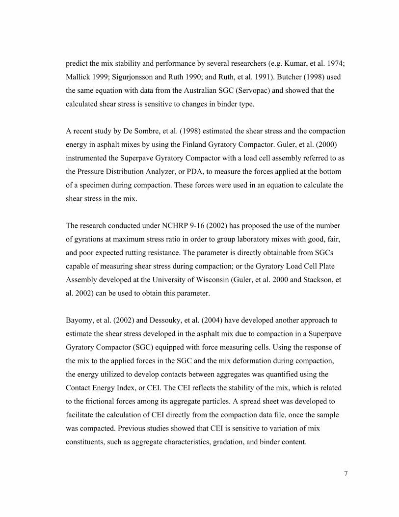
of one of the load cells, as shown in Figure 2.3 and Equations 2.10 – 2.12.
eM xx ⇒=Σ 0 (2.10)
eM yy ⇒=Σ 0 (2.11)
15
)(2
2 e yr yexe −+= (2.12)
where,
Mx is the moment around x-axis,
My is the moment around y-axis,
ex, ey are x and y components of eccentricity e respectively, and
ry is the location of plate center point with respect to coordinate axis.
Figure 2.3 Free Body Diagram to Determine ex and ey
The PDA can be placed in the Servopac compactor, and the forces obtained directly
from Servopac, and from the PDA, can be used to calculate GS. As shown in Figure 2.4,
the GS values, whether determined from the Servopac data or by the PDA, are almost
identical.
2.4.2. Troxler SGC and PDA
In order to examine the influence of the compactor type on GS results, twelve of the
mixes were compacted using the Troxler (Model 4140) Superpave Gyratory Compactor,

16
equipped with the PDA plate. All samples per mix have yielded approximately the same
GS values, as shown in Figure 2.5, irrespective of the compactor type. The minor
discrepancy of results can be attributed to the random variability in the mix batches and
in the laboratory operations, since the samples compacted with the Troxler compactor
were done at the ITD Central Laboratory, while those compacted by the Servopac were
prepared at the University of Idaho. The results indicate that the PDA can be used to
obtain the compaction forces and calculate GS.
n = 6 5 , R2 = 0 .9 9 3 2
0
5
10
15
20
25
30
0 5 10 15 20 25 30
G S , k N.m - Us ing S ervopac S G C
GS
, kN
,m -
Usi
ng P
DA
Figure 2.4 Comparison between GS Values Calculated Using Servopac and PDA

17
n = 11, R2 = 0.6546
10
12
14
16
18
20
22
24
26
28
30
15 17 19 21 23 25
G S , k N.m - Us ing S ervopac S G C
GS
, kN
.m -
Usi
ng T
roxl
er S
GC
+ P
DA
Figure 2.5 Comparison between GS Values Calculated Using Servopac and
Troxler Compactors
2.4.3. Pine SGC
The Pine Instrument AFG1A SGC is designed to compact prepared HMA specimens at a
constant consolidation pressure, a constant angle of gyration, and at a fixed speed of
gyration (Dalton 2004). The Pine AFG1 compactor is equipped with a shear
measurement system, which records the shear stress in terms of a unitless Gyratory
Shear Ratio once per gyration. The Gyratory Shear Ratio is automatically recorded each
time an HMA specimen is compacted, and the shear data can be recovered from the data
file generated by the Pine AFG1A SGC. No special setting is required.
During the compaction process in the Pine AFG1A SGC, the compactor’s ram applies a
force (R) to the bottom plate as shown in Figure 2.6. This ram force is opposed by an
equal but opposite force at the fixed top plate. Given the cross-sectional area of the mold
(A), the ram pressure (P) can be computed as follows:
ARP = (2.13)

18
Figure 2.6 Simple Shear Diagram (Dalton 2004)
Further, to achieve the gyration angle during compaction, a vertical force (F) is applied.
The force would vary based on the lever arm distance (d), the mix stiffness, the
specimen volume (V), and the ram pressure. The Shear Stress may be determined by
Equation 2.14 (Dalton 2004).
V
dFS .= (2.14)
The Pine AFG1A SGC computes and reports the Gyratory Shear Ratio (σ) in its output,
in addition to the changes in height, vertical pressure, and the gyration angle.
PS
=σ (2.15)
These parameters are essential in calculating GS; therefore, the Pine AFG1A SGC has a
high potential to be used for this purpose. Unfortunately, the Pine technical center was
not able to provide the research team with the location of the force sensors in the Pine
AFG1A SGC or the value of the level arm (d), which are essential to back-calculate the

19
actual shear force generated in the HMA specimen during compaction, excluding the
machine losses.
Therefore, it was decided to adopt a practical approach, by studying the forces diagram
in the Pine SGC (Figure 2.6). It was found that it is very similar to the forces diagram in
Servopac SGC used in determining GS (Figure 2.1). The only difference between the
two compactors is how the gyration angle is applied (F). Pine SGC uses two pistons to
apply the gyration angle, while the Servopac SGC uses three. If the shear stress
computed using the Pine SGC could be correlated to the shear stress computed using the
Servopac SGC, then there would be no need to revise the GS calculation procedure.
Instead, the computed, correlated (modified) shear stress could be used directly.
The first step of this analysis was to determine if the forces applied on the specimen in
the Pine AFG1A and the Servopac SGCs are the same, using the final air voids (AV %)
as the criterion to compare the two compactors. It was found that the AV% for each mix,
regardless of the SGC type, yielded approximately the same AV% (Figure 2.7). The
minor discrepancy of results can be attributed to the random variability in the mix
batches and in the laboratory operations. Thus, it can be assumed that the resultant
applied forces are the same.
Then, the shear stresses computed by each compactor for the same mix were compared,
and it was observed that these stresses follow the same trend (Figure 2.8), except that
shear stresses computed by the Pine SGC are higher.

20
n =22, R2 = 0.9204
0
2
4
6
8
10
12
0 2 4 6 8 10 12AV%, Servopac SGC
AV
%, P
ine
SG
C
Figure 2.7 AV% Using Pine versus Servopac SGCs
0
100
200
300
400
500
600
0 20 40 60 80 100 120 140 160 180
Gyration, N
She
ar S
tress
, kP
a Pine
Servopac
Figure 2.8 Comparison of Shear Stress Determined by Pine and Servopac SGCs
After a close examination, the shear stress computed by the Pine SGC seemed to
correlate to the shear stresses computed by the Servopac. Thus, a numerical model was
developed. It can be expressed as follows:
BSSASS PineServopac += . (2.16)

21
where,
SSServopac is the shear stress determined by Servopac SGC,
SSPine is the shear stress determined by Pine SGC, and
A and B are regression parameters and are equal to 0.82 and -52.14 respectively.
As a final step, using the modified shear stress computed by the Pine, the GS was
calculated for all mixes, and compared to the GS values determined using the shear
stress computed by the Servopac SGC. As shown in Figure 2.9, the GS values are
approximately equal for the same mix. The minor differences are believed to be due to
the variability in the mix batches and in the laboratory operations.
n = 16, R2 = 0.8808
15
16
17
18
19
20
21
15 16 17 18 19 20 21
GS by Servopac, kN.m
GS
by P
ine
(AFG
1) ,
kN.m
Figure 2.9 Gyratory Stability Calculated by Servopac and Pine SGC
2.5. SUMMARY
This research defines the Gyratory Stability (GS) as the same value as the Contac
Energy Index (CEI), but measured between number of gyrations NG1 and N-design. The
gyration number NG1 is determined based on an established criterion, which identifies the

22
compaction point when the mix shear resistance starts to develop, and increases with
more aggregate contacts. N-design is the number of gyrations defined by the Superpave
system. For Hveem-designed mixes, N-design is considered to be the gyration at which
the compacted mix reaches 4% air voids. Conclusions and observations on the
evaluation of Gyratory Stability are the following:
The mix GS is a simple and quick parameter for measuring the mix stability. It is
reproducible and independent of the compactor type.
GS can be determined using a shear-measurement-capable compactor with little
modification. For an SGC with no shear measurement capacity, an external plate (i.e.
PDA) can be used to determine the forces developed in the mix during compaction.

This is a Blank Page

23
3. EXPERIMENTAL PROGRAMS USING IDAHO MIXES
3.1. INTRODUCTION
The experimental phase of this project involved two prgrams. First that involves Hveem
designed mixes, and the second involves Superpave mixes. The overall objective of the
Hveem mixes experimental program was to apply the Gyratory Stability concept on as
many mixes as we could obtain, to represent the various mix conditions in the state of
Idaho. At the beginning of the project, all Idaho mixes were designed in accordance with
the Hveem design method. Near the end of the project period, however, ITD had begun
construction of a few Superpave mixes in various parts of the state. Therefore, the mix
evaluation process involved two groups of mixes: one group evaluated Hveem-designed
and constructed mixes, and the second group evaluated Superpave mixes. These mixes
were collected from the field sites at the time of construction. In order to not disturb the
construction operation, mix samples were collected from the truck at the paver feeder in
accordance with standard ITD sample collection methods. In this chapter, a description
of the mixes used in this study, and their design parameters, are described for both mix
groups.
3.2. HVEEM DESIGNED MIXES
In cooperation with the Idaho Transportation Department (ITD), fifty-two different
mixes of HMA, designed and constructed in accordance to the Hveem method, were
procured from various project sites located in Idaho. Figure 3.1 shows a map for the
general geographical locations of the projects where these mixes were collected.
Although these mixes were designed in accordance with the Hveem method, their
binders were designed in accordance to the Superpave PG grading system. These mixes
varied in their aggregate types, gradations (Mix Class I, II and III as per ITD general

24
specifications (2004)), binder grade (PG 76-28, PG 70-28, PG 64-34, PG 64-28, PG 58-
34, and PG 58-28), and binder content (3.3% - 6.1%). Mixes were selected to cover a
wide range of Hveem stability values and various mix classes that are produced in Idaho.
Most of the tests were performed on field batches as they were provided by the state
engineer. Some of the mixes were duplicated in the laboratory and modified to test the
effect of mix properties, such as asphalt content and binder grade, on Gyratory Stability
(GS). Table 3.1, Table 3.2 and Table 3.3 describe the main characteristics of the selected
mixes. Details about these mixes are documented in Appendix A “Mix design and Job
Mix Formula (JMF) for all mixes.”
Field batches for the mixes were tested to confirm their Hveem design parameters, and,
using the SGC, samples were prepared in order to calculate GS values, as well as for
Asphalt Pavement Analyzer (APA) and Fracture Toughness (Jc) testing. Samples were
compacted, and the GS values for all mixes were calculated at the UI asphalt lab.
For the purpose of investigating whether GS correlated with Hveem stability, all
specimens were compacted to a number of gyrations to produce samples with 4% air
void (the design target for Hveem criteria). However, the maximum number of gyrations
applied was limited to 250. In the case of coarser mixes, where 4% air void was not
achievable, even at 250 gyrations, that sample was eliminated from the population used
for Hveem stability correlation.
Details about these mixes are documented in Appendix A. Compaction data files are
provided on the attached CD as Appendix B.

25
Figure 3.1 Idaho Counties and the Locations of Procured HMA Mixes

26
Table 3.1 Properties of Selected Field and Lab Modified Hveem Mixes (Class I)
Mix Class Binder Grade
% AC Mix Designation
Jc
Testing APA Testing
4.20 G24-L
(-1% AC) √
G24 √ √ 5.20
G24-L √ √
5.50 G08 √
76-28
5.55 G21 √ √
4.80 G05 √
5.16 G01 √
G02 √ 5.30
G03 √
70-28
5.5 G45-G48
64-34 3.90 G10 √
5.20 G18 √
G18-L √ 5.20
5.80 G26 √ √
64-28
4.90 G03 √
G04 √
5.30 G06 √
G09 √ 5.30
5.44 G22 √ √
5.50 G49
5.70 G32 √ √
58-34
5.30 G16 √
4.40 G44
4.90 G36
5.10 G37-G43
I
58-28
5.90 G11 √

27
Table 3.2 Properties of Selected Field and Lab Modified Hveem Mixes (Class II)
Mix Class Binder Grade
% AC Mix Designation
Jc Testing APA Testing
76-28 5.65 G20-L
(76-28) √
64-34 4.70 G34 √
5.00 G07 √
G20 √ √ 64-28
5.65 G20-L
(64-28) √ √
3.30 G29-L
(-1% AC) √
4.20 G15 √
G25 √ √
G29 √ √
G29-L √ √
G30 √
4.30
G31 √ √
5.30 G29-L
(+1% AC) √
58-34
5.65 G20-L
(58-34) √
G23 √ √ 4.80
G35 √
5.10 G17 √
II
58-28
5.65 G20-L
(58-24) √

28
Table 3.3 Properties of Selected Field and Lab Modified Hveem Mixes (Class III)
Mix Class Binder Grade
% AC Mix designation
Jc testing APA testing
G12 √
G13 √ 64-34 4.30
G14 √
G27 √ √ 5.80
G27-L √ √
5.90 G19 √
III
58-28
6.10 G28 √ √
3.3. SUPERPAVE DESIGNED MIXES
The Idaho Transportation Department implemented the Superpave PG binder
specifications several years ago, and recently utilized the Superpave mix design on a few
projects in the state. In cooperation with ITD, raw materials from two different
Superpave design mixes were obtained. These mixes were duplicated in the laboratory
and were modified in order to study the effect of the mix properties, such as asphalt
content and binder grade, on the performance of the mix.
Samples were compacted using the SGC in order to calculate their GS values. Then,
samples were prepared for Asphalt Pavement Analyzer (APA), Fracture Toughness (Jc),
Dynamic Modulus (E*), and Flow Number (Fn) testing. For the purpose of investigating
whether GS correlated to Superpave specifications, samples at optimum conditions were
compacted to N-design as specified by the Superpave mix design for Superpave mixes.
However, for Hveem mixes, the samples were compacted to varied number of gyrations
to produce specimens with 4% air voids, which is the design target for Superpave mix
design. In any case, the number of Gyrations was limited to maximum of 250 if the 4%
air voids was not achieved. Table 3.4 describes these mixes and the applied alterations.

29
Details about these mixes are documented in Appendix A. Compaction data files are
provided on the attached CD in Appendix B.
Table 3.4 Properties of Selected Field and Lab Modified Superpave Mixes
Mix Binder Grade
% AC Jc Testing APA Testing
E* and Fn
Testing
5.0 (-0.5
AC%) √ √ √
5.5 (opt.
AC%) √ √ √
6.0 (+0.5
AC%) √ √ √
Mix 1 64-34
6.5 (+1.0
AC%) √ √ √
5.0 (-1.0
AC%) √ √
5.9 (opt.
AC%) √ √ √ 64-28
7.0 (+1.0
AC%) √ √ √
64-22 5.9 (opt.
AC%) √ √ √
Mix 2
64-34 5.9 (opt.
AC%) √ √ √

This is a Blank Page

30
4. EVALUATION OF AGGREGATE TEXTURE AND SHAPE PROPERTIES USING IMAGE ANALYSIS
4.1. DEFINITION OF AGGREGATE SHAPE
Researchers have distinguished between the different aspects that constitute particle
geometry. Particle geometry can be fully expressed in terms of three independent
properties: form, angularity (or roundness), and surface texture. Figure 4.1 shows a
schematic diagram that illustrates the differences between these properties. Form, the
first order property, reflects variations in the proportions of a particle. Angularity, the
second order property, reflects variations at the corners; that is, variations superimposed
on shape. Surface texture is used to describe the surface irregularity at a scale that is too
small to affect the overall shape. These three properties can be distinguished because of
their different scales with respect to particle size, and this feature can also be used to
order them. Any of these properties can vary widely without necessarily affecting the
other two properties.
Form
Angularity
Texture
Figure 4.1 Components of an Aggregate Shape: Form, Angularity, and Texture
31
4.2. AIMS OPERATIONS
Details of the main components and design of the prototype Aggregate Imaging System
(AIMS) have been reported by Masad (2003). Researchers developed AIMS to capture
images and analyze the shape of a wide range of aggregate types and sizes, which
represent those used in asphalt mixes, hydraulic cement concrete, and unbound
aggregate layers of pavements. AIMS uses a simple setup that consists of one camera
and two different types of lighting schemes to capture images of aggregates at different
resolutions, from which aggregate shape properties are measured using image analysis
techniques.
The system operates based on two modules. The first module is for the analysis of fine
aggregates (smaller than 4.75 mm (#4)), where black and white images are captured. The
second module is devoted to the analysis of coarse aggregates (larger than 4.75 mm
(#4)). In the coarse module, gray images as well as black and white images are captured.
Combining both the coarse and fine aggregate analysis into one system is considered
advantageous, due to the reduced cost of developing the system. It also allows the use of
the same analysis methods to quantify aggregate shapes, irrespective of their size, to
facilitate relating aggregate shape to pavement performance.
Fine aggregates are analyzed for form and angularity using black and white images,
which are captured using backlighting under the aggregate sample tray. This type of
lighting creates a sharp contrast between the particle and the tray, thus giving a distinct
outline of the particle. A study by Masad, et al. (2001) clearly shows that a high
correlation exists between the angularity (measured on black and white images) and
texture (measured on gray scale images) of fine aggregates. Therefore, only black and
white images are used to analyze fine aggregates.
AIMS is designed to capture images for measuring fine aggregate angularity and form at
a resolution such that a pixel size is less than 1 percent of the average aggregate

32
diameter, and the field of view covers 6-10 aggregate particles (Masad, et al. 2000). In
other words, the resolution of an image is a function of aggregate size. The image
acquisition setup is configured to capture a typical image of 640 by 480 pixels at these
resolutions in order to analyze various sizes of fine aggregates.
For coarse aggregates, researchers have found that there is a distinct difference between
angularity and texture, and these properties have different effects on performance
(Fletcher, et al. 2003). Consequently, AIMS analyzes coarse aggregates for shape and
angularity using black and white images, and analyzes texture using gray images. A
backlighting table is used to capture the black and white images, while a top lighting
table captures gray images of particles surfaces. As for fine aggregates, the image
acquisition setup captures images of 640 by 480 pixels. In the coarse aggregate module,
only one particle is captured per image in order to facilitate the quantification of form,
which is based on three-dimensional (3-D) measurements. As described later in this
chapter, the use of the video microscope determines the depth of a particle, while the
images of two-dimensional projections provide the other two dimensions to quantify
form. Texture is determined by analyzing the gray images, using the wavelet method
described later.
AIMS utilizes a closed-loop DC servo control unit of the x, y, and z axes for precise
positioning and highly repeatable focusing. The x and y travel distance is 37.5 cm (15
inches); and the z travel distance is 10 cm (4 inches). The external controller is housed in
a small 15 x 10 cm (6 x 4 inches) case.
The Optem Zoom 160 video microscope is also used in AIMS. The Zoom 160 has a
range of X16, which means that an image can be magnified by 16 times. This
magnification allows for the capture of a wide range of particle sizes without changing
parts. AIMS is equipped with a Pulnix TM-9701 progressive scan video camera with a
16.9 mm (2/3 inch) CCD imager. It has an adjustable shutter speed from 1/60 s to

33
1/16000 s. The progressive scan video camera captures images at a higher speed than
line scan cameras, and it is less affected by noise.
AIMS is equipped with both bottom lighting and top lighting, composed of a ring
mounted on the video microscope (Figure 4.2). The ring light provides uniform
illumination of the region directly in the view of the microscope.
Figure 4.2 Top Lighting Used in AIMS
4.2.1. Fine Aggregate Module Operation Procedure
The analysis of fine aggregates starts by randomly placing an aggregate sample (ranging
from a few grams for small fine aggregate sizes, up to a couple of hundred grams for the
larger fine aggregate size) on the aggregate tray with the backlighting turned on. A
camera lens of 0.5X objective is used to capture the images. The 0.5X objective lens will
provide a field of view of 26.4 x 35.2 mm with a 1X Dovetail tube and a 2/3 foot camera
format at a working distance of 181 mm. The camera and video microscope assembly
moves incrementally in the x direction at a specified interval, capturing images at every
increment. Once the x-axis range is complete, the aggregate tray moves in the y-
direction for a specified distance, and the x-axis motion is repeated. This process
continues until the whole area is scanned.
34
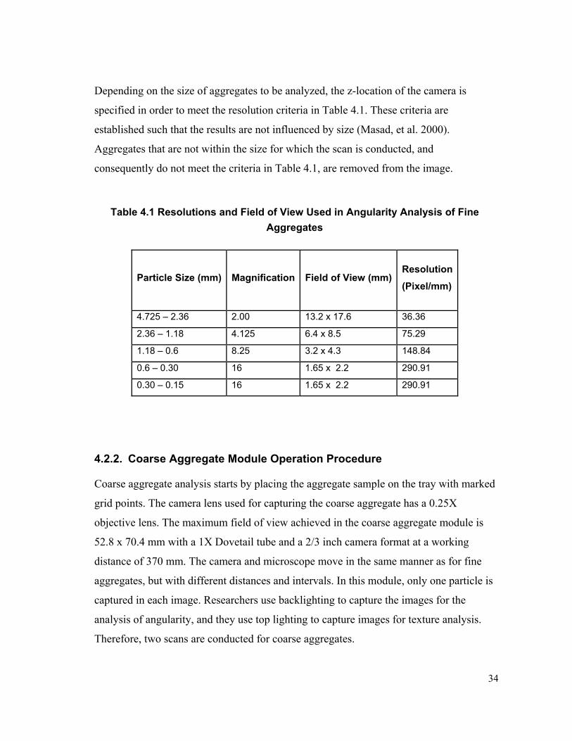
Depending on the size of aggregates to be analyzed, the z-location of the camera is
specified in order to meet the resolution criteria in Table 4.1. These criteria are
established such that the results are not influenced by size (Masad, et al. 2000).
Aggregates that are not within the size for which the scan is conducted, and
consequently do not meet the criteria in Table 4.1, are removed from the image.
Table 4.1 Resolutions and Field of View Used in Angularity Analysis of Fine Aggregates
Particle Size (mm) Magnification Field of View (mm)Resolution (Pixel/mm)
4.725 – 2.36 2.00 13.2 x 17.6 36.36
2.36 – 1.18 4.125 6.4 x 8.5 75.29
1.18 – 0.6 8.25 3.2 x 4.3 148.84
0.6 – 0.30 16 1.65 x 2.2 290.91
0.30 – 0.15 16 1.65 x 2.2 290.91
4.2.2. Coarse Aggregate Module Operation Procedure
Coarse aggregate analysis starts by placing the aggregate sample on the tray with marked
grid points. The camera lens used for capturing the coarse aggregate has a 0.25X
objective lens. The maximum field of view achieved in the coarse aggregate module is
52.8 x 70.4 mm with a 1X Dovetail tube and a 2/3 inch camera format at a working
distance of 370 mm. The camera and microscope move in the same manner as for fine
aggregates, but with different distances and intervals. In this module, only one particle is
captured in each image. Researchers use backlighting to capture the images for the
analysis of angularity, and they use top lighting to capture images for texture analysis.
Therefore, two scans are conducted for coarse aggregates.

35
Backlighting is used in order to capture black and white images. These images are
analyzed later to determine angularity, and the major (longest) and minor (shortest) axes
on these two-dimensional images. The analysis of coarse aggregate angularity starts by
placing the aggregate particles in a grid pattern with a distance of 50 mm in the x-
direction and 40 mm in the y-direction from center to center. The z-location of the
camera is fixed for all aggregate sizes. Table 4.2 presents image resolutions used in the
coarse aggregate angularity analysis.
Table 4.2 Resolutions and Field of View Used in Angularity Analysis of Coarse Aggregates
Particle Size (mm) Magnification Field of View (mm) Resolution (pixel/mm)
9.5 – 4.725 1 52.8 X 70.4 9.12
12.7 – 9.5 1 52.8 X 70.4 9.12
19.0 – 12.7 1 52.8 X 70.4 9.12
25.4 – 19.0 1 52.8 X 70.4 9.12
> 25.4 1 52.8 X 70.4 9.12
Capturing images for the analysis of coarse aggregate texture is very similar to the
angularity analysis except that top lighting is used instead of backlighting, in order to
capture gray images. The texture scan starts by focusing the video microscope on a
marked point on the lighting table while the backlighting is turned on. The location of
the camera on the z-axis at this point is considered as a reference point (set to zero
coordinate). Then an aggregate particle is placed over the calibration point. With the top
light on, the video microscope moves up automatically on the z-axis in order to focus on
the aggregate surface. The z-axis coordinate value on this new position is recorded.
Since the video microscope has a fixed focal length, the difference between the z-axis
coordinate at the new position and the reference position (zero) is equal to aggregate
depth. This procedure is repeated for all particles. The particle depth is used, along with
36
the dimensions measured on black and white images, to analyze particle shape or form
as discussed later.
4.3. AIMS ANALYSIS METHODS
4.3.1. Texture Analysis Using Wavelets
Wavelet analysis is a powerful method for describing the decomposition of the different
scales of texture in aggregate samples (Mallat 1989). In order to isolate fine variations
in texture, very short-duration basis functions should be used. At the same time, very
long-duration basis functions are suitable for capturing coarse details of texture. These
measurements are accomplished in wavelet analysis by using short high-frequency basis
functions and long low-frequency ones. The wavelet transform works by mapping an
image onto a low-resolution image and a series of detailed images. The low-resolution
image is obtained by iteratively blurring the original images, eliminating fine details in
the image while retaining the coarse details. The remaining detailed images contain the
information lost during this operation. The low-resolution image can be further
decomposed into the next level of low resolution and detailed images.
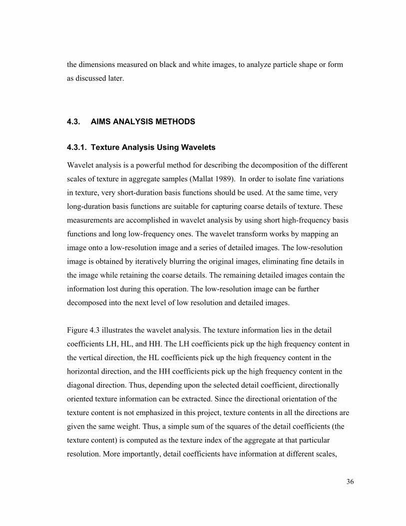
Figure 4.3 illustrates the wavelet analysis. The texture information lies in the detail
coefficients LH, HL, and HH. The LH coefficients pick up the high frequency content in
the vertical direction, the HL coefficients pick up the high frequency content in the
horizontal direction, and the HH coefficients pick up the high frequency content in the
diagonal direction. Thus, depending upon the selected detail coefficient, directionally
oriented texture information can be extracted. Since the directional orientation of the
texture content is not emphasized in this project, texture contents in all the directions are
given the same weight. Thus, a simple sum of the squares of the detail coefficients (the
texture content) is computed as the texture index of the aggregate at that particular
resolution. More importantly, detail coefficients have information at different scales,

37
depending upon the level of decomposition. Multi-resolution (or scale) analysis is a very
powerful tool that is not possible using a regular Fourier transform.
To describe the texture content at a given resolution or decomposition level, a parameter
called the wavelet texture index is defined. The texture index at any given
decomposition level is the arithmetic mean of the squared values of the detail
coefficients at that level:
( )( )
23
,1 1
1 (Wavelet Method) ,3
N
n i ji j
Texture Index D x yN = =
= ∑∑ (4.1)
where,
n refers to the decomposition level,
N denotes the total number of coefficients in a detailed image of texture,
i takes values 1, 2, or 3, for the three detailed images of texture,
j is the wavelet coefficient index, and
(x, y) is the location of the coefficients in the transformed domain.
In this project, the texture is decomposed to six levels. However, only the results from
level 6 are used since previous research has shown that level 6 is the least affected by
color variations and the presence of dust particles on the surface (Masad 2003).

38
Figure 4.3 Two-level Wavelet Transformation
4.3.2. Angularity Analysis Using Gradient Method
In order to measure angularity, one needs a method that assigns a finite value of
angularity to a highly angular particle with sharp angular corners, and simultaneously
assigns near-zero angularity to a well-rounded particle. In addition, the method should
be capable of distinguishing those particle shapes that have angularities between these
two extremes, but which appear similar to the naked eye. The gradient method,
described below, possesses both of these properties.
The gradient-based method for measuring angularity starts by calculating the gradient
vectors at each edge-point using a Sobel mask, which operates at each point on the edge
and its eight nearest neighbors. The gradient of an image ( )yxf , at location ( )yx, is the
vector:
⎥⎥⎥⎥⎥
⎦
⎤
⎢⎢⎢⎢⎢
⎣
⎡
∂∂
∂∂
=⎥⎥⎥
⎦
⎤
⎢⎢⎢
⎣
⎡
=∇
yf
xf
G
Gf
y
x
(4.2)
Pixel
Values
WaveletTransformation
Original Image
Detail Coefficients for 1st level
Transformed Image
L H
H
H
L H
L

39
It is known from vector analysis that the gradient vector points in the direction of the
maximum rate of change of f at ( )yx, . The magnitude of the vector is given by f∇ ,
where:
( ) [ ]2122yx GGfmagf +=∇=∇ (4.3)
The direction of the gradient vector can be represented by the angle ( )yx,θ of the
vector f∇ at ( )yx, :
( ) ⎟
⎟⎠
⎞⎜⎜⎝
⎛= −
y
x
GG
yx 1tan,θ (4.4)
where the angle is measured with respect to the x axis.
It should be noted that computation of the gradient of an image is based on calculating
the partial derivatives xf∂∂
and yf∂∂
at every pixel location. These derivatives are
implemented in the discrete domain using the Sobel operator, which has the advantage
of providing both a differentiating and a smoothing effect. The smoothing effect is
particularly useful because the derivative operation has the effect of enhancing noise. At
sharp corners of the edges of a particle image, the direction of the gradient vector
changes rapidly. On the other hand, the direction of the gradient vector for rounded
particles changes slowly for adjacent points on the edge.
For the angularity analysis of aggregates, researchers use the angle of orientation values
( )θ of the edge-points, and the magnitude of the difference in these values ( )θΔ for
adjacent points on the edge, to describe how sharp (large θΔ ) or how rounded (small
θΔ ) the corner is. Based on the orientation of the gradient-vectors at each edge-point,
the angularity index is calculated for the aggregate particle. Angularity values for all
boundary points are calculated, and their sum accumulated around the edge, to form the

40
angularity index of the aggregate particle. The angularity index can be represented
mathematically as:
3
31
(Gradient Method)N
i ii
Angularity Index θ θ−
+=
= −∑ (4.5)
where,
the subscript i denotes the thi point on the edge of the particle, and
N is the total number of points on the edge of the particle.
The step-size used in this project was 3. That is, the angle of orientation of every third
point on the boundary of the aggregate was used to form the angularity index. This value
was determined empirically to be optimum, given the resolution of the edge of the
images used in the project.
4.3.3. Form Analysis Using Sphericity
Information about the three dimensions of a particle, namely the longest dimension,
(dL), the intermediate dimension (dI), and the shortest dimension (ds) is essential for
proper 3-D characterization of the aggregate form. Sphericity is defined in terms of these
three dimensions as shown in Equation 4.6:
Sphericity3
2L
ls
dd.d
= (4.6)
AIMS uses the auto focus microscope to measure the depth of a particle, while the two-
dimensional projections are analyzed using eigenvector analysis to determine the
principal axes. In this method, the binary image of the aggregate is treated as a two-
41
dimensional population. Each pixel in the population is treated as a two-dimensional
vector ( )Tbax ,= , where a and b are the coordinate values of that pixel with respect to x and y axes. These vectors are used to compute the mean vector and covariance
matrix of the population. The eigenvectors of the covariance matrix are computed, which
are orthogonal to each other. The major and minor axes (or the longest and intermediate
axes in this case) of the object (aggregate) are aligned along these eigenvectors. Since it
is easy to find the centroid of the aggregate, the length of the axes is the same as the
distance from the centroid of the aggregate to the edge along the two axes
(eigenvectors). This method gives major and minor axes on the projection. These axes
with the particle thickness are used to calculate the sphericity in Equation 4.6.
4.4. AGGREAGTE SHAPE CLASSIFICATION
A comprehensive methodology for classification of aggregates based on the distribution
of their shape characteristics should exhibit the following features:
• It represents the three characteristics of aggregate shape (three dimensions of
coarse aggregates, angularity, and texture).
• It unifies the methods used to measure the shape characteristics of fine and
coarse aggregates.
• Similar to what is currently done for aggregate gradation, each of the shape
characteristics is represented by a cumulative distribution function rather than an
average value. Therefore, the methodology is capable of accommodating variations
in shape within an aggregate sample, and better represents the effects of different
processes such as blending and crushing on aggregate shape.

42
• It is developed based on statistical analysis of a wide range of aggregate types
and sizes.
The classification methodology criteria, described above, arose from measuring the
shape characteristics of aggregates from a wide range of sources and varying sizes using
AIMS. The analysis generated a total of 195 tests on coarse aggregates and 75 tests on
fine aggregates. On average, a coarse aggregate test involved 56 particles, while a fine
aggregate test involved about 300 particles. All of this data was used in the development
of the new classification system.
Researchers used cluster analysis to develop groups (or clusters) of aggregates based on
the distribution of shape characteristics. Clustering is a widely used pattern recognition
method for grouping data and variables. Grouping is done on the basis of similarities or
differences. In many areas of engineering and science, it is important to group items into
natural clusters. Basic references about clustering methods include most applied
multivariate statistical texts (e.g., Johnson and Wichern, 2002; and Morrison, 2005). All
clustering methods begin with a choice of a metric (a distance or closeness among
objects) and a choice of a method for grouping objects.
The clustering method was applied to the analysis results of each shape property
obtained from AIMS. The research team found that groups or clusters can be developed
for each of the shape properties, irrespective of aggregate size. Figure 4.4 shows the
developed classification limits. More details on the development of the classification
methodology are available in Al-Rousan, et al. (2005).
The sphericity value gives a very good indication of the proportions of particle
dimensions. However, one cannot determine whether an aggregate has flat, elongated, or
flat and elongated particles using sphericity alone. To resolve this, the analysis shown in
the chart in Figure 4.5 is included in the AIMS software to distinguish among flat,

43
elongated, and flat and elongated particles. Superimposed on this chart are the 3:1 and
5:1 limits for the longest to shortest dimension ratio. The use of this chart is illustrated
here, with the aid of the results from two aggregate samples denoted CA-2 and CA-4.
Both aggregates CA-2 and CA-4 pass the 5:1 Superpave requirement (both had less than
10 percent content with a particle dimensional ratio of 5:1), but they had distinct
distributions in terms of flat and elongated particles.
This type of analysis, shown in Figure 4.5, reveals valuable information about the
distribution, which would not have been obtained if aggregates were classified based on
the ratio of 5:1 only. Such details are needed to understand the influence of shape
characteristics on asphalt mix performance. It is believed that some of the discrepancies
in the literature with regard to the influence of shape on performance are attributed to the
lack of such details; plus the reliance on indirect methods of measuring average indices
to describe shape.

44
Rou
nded
Sub
Rou
nded
Sub
Angu
lar
Angu
lar2100 4000 5400
Flat
/Elo
ngat
ed
Low
Sp
heric
ity
Mod
erat
e Sp
heric
ity
Hig
h Sp
heric
ity
0.6 0.7 0.8
Polis
hed
Smoo
th
Low
R
ough
ness
Mod
erat
e R
ough
ness
Hig
h R
ough
ness165 275 350 460
Figure 4.4 Aggregate Shape Classification Chart
Angularity
Form
(Sphericity)
Texture

45
0
0.1
0.2
0.3
0.4
0.5
0.6
0.7
0.8
0.9
1
0 0.1 0.2 0.3 0.4 0.5 0.6 0.7 0.8 0.9 1
Short/ Intermediate = Flatness Ratio
Inte
rmed
iate
/ Lon
g =
Elon
gatio
n R
atio
CA-2
CA-4
SP=0.5
SP=0.6
SP=0.7
SP=0.8
1 : 5 1 : 3
Figure 4.5 A Chart for Identifying Flat, Elongated, or Flat and Elongated Aggregates
4.5. ANALYSIS OF IDAHO AGGREGATES
Each coarse aggregate was sieved, and each coarse aggregate size with at least 56
particles was imaged and analyzed. The coarse aggregate analysis included texture,
angularity and form. Statistical parameters (average and standard deviation) were also
Flatness decreases
Elo
ngat
ion
decr
ease
s
Ratio of shortest to longest axes (Superpave Limits)

46
calculated for each of the aggregate sizes. The fine aggregates were also sieved and
aggregates retained on sieves #8, #16, #30, and #60 were imaged and analyzed. The
distributions of the shape characteristics for each aggregate size are given in the
accompanying CD. The AIMS workbooks are programmed to facilitate the generation of
graphical representations of the data and comparisons among different aggregates. For
the sake of simplicity, the combined average and standard deviation for the different
sizes from the fine and coarse fractions of each aggregate source were calculated. These
values are shown in Tables 4.3 and 4.4 and Figures 4.6- 4.12. The following points
summarize the main findings from these results:
• Coarse aggregates vary significantly in their texture. Mix 2 includes coarse
aggregates with the highest texture compared with the other mixes (Figure 4.6).
• Mix 1 has coarse aggregates with the highest angularity (Figure 4.7). This high
angularity can compensate for the relatively low texture of these aggregates.
• Mix 3 has the lowest angularity and texture. This mix can be susceptible to
rutting, due to these unfavorable aggregate characteristics.
• Coarse aggregates of Mix 3 and aggregates from stockpile B of Mix 2 have the
lowest sphericity values (Figure 4.8). These low sphericity values reflect the high
percentage of particles with the longest to shortest dimension ratios, greater than
3:1 and greater than 5:1, as evident in the results shown in Figures 4.9 and 4.10.
As would be expected from the definition of sphericity in Eq. 4.6, there is a very
good correlation between sphericity and the percentage of particles with longest
to shortest dimension ratios greater than 5:1 and 3:1 (Figure 4.11).
• There is wide variation in the angularity of fine aggregates. The sand used in Mix
2 has the lowest angularity (Figure 4.12)

16
Tabl
e 4.
3 Su
mm
ary
of th
e Sh
ape
Cha
ract
eris
tics
of C
oars
e A
ggre
gate
s
Text
ure
A
ngul
arity
-Gra
dien
t Sp
heric
ity
%
Part
icle
s L/
S>3
% P
artic
les
L/S>
5 A
ggre
gate
Lab
el
Ave
rage
St
. Dev
Ave
rage
St
. Dev
A
vera
ge
St. D
ev
G19
-765
0_C
lass
_Mix
_3
124.
54
53.9
8 28
29.9
8 14
41.0
8 0.
58
0.12
56
.70
20.6
0
G20
-848
6_C
lass
_Mix
_2_P
ile_A
20
5.96
47
.56
3414
.64
1449
.06
0.65
0.
11
34.5
0 5.
50
G20
-848
6_C
lass
_Mix
_2_P
ile_B
11
9.70
44
.81
3504
.20
1603
.11
0.59
0.
12
59.0
0 20
.50
G20
-848
6_C
lass
_Mix
_2_P
ile_C
10
8.77
33
.04
2684
.80
1286
.58
0.65
0.
10
36.6
0 2.
70
G22
-832
7_M
ix_C
lass
_1_P
ile_A
20
6.32
53
.79
4062
.62
1520
.30
0.61
0.
10
46.8
0 7.
20
G22
-832
7_M
ix_C
lass
_1_P
ile_B
14
7.86
45
.67
3951
.78
1418
.58
0.60
0.
11
23.4
0 5.
40
G29
-706
8_C
lass
_Mix
_2
190.
21
96.8
4 29
50.8
4 14
29.2
8 0.
71
0.10
12
.60
1.20

17
Ta
ble
4.4
Sum
mar
y of
the
Ang
ular
ity o
f Fin
e A
ggre
gate
s
Ang
ular
ity-G
radi
ent
Agg
rega
te L
abel
Ave
rage
St
. Dev
G19
-765
0_C
lass
_Mix
_3
3724
.82
1594
.66
G20
-848
6_C
lass
_Mix
_2_S
and
3122
.30
1439
.88
G20
-848
6_C
lass
_Mix
_2_P
ile_C
42
09.8
0 17
47.4
2
G22
-832
7_M
ix_C
lass
_1_P
ile_C
41
64.9
7 16
77.9
9
G29
-706
8_C
lass
_Mix
_2
3442
.01
1567
.04

43
0.00
50.00
100.00
150.00
200.00
250.00
300.00
350.00
G19-76
50_C
lass_
Mix_3
G20-84
86_C
lass_
Mix_2_
Pile_A
G20-84
86_C
lass_
Mix_2_
Pile_B
G20-84
86_C
lass_
Mix_2_
Pile_C
G22-83
27_M
ix_Clas
s_1_
Pile_A
G22-83
27_M
ix_Clas
s_1_
Pile_B
G29-70
68_C
lass_
Mix_2
Aggregate Source
Text
ure
Inde
x
Figure 4.6 Texture of Coarse Aggregates
0.00
1000.00
2000.00
3000.00
4000.00
5000.00
6000.00
G19-76
50_C
lass_
Mix_3
G20-84
86_C
lass_
Mix_2_
Pile_A
G20-84
86_C
lass_
Mix_2_
Pile_B
G20-84
86_C
lass_
Mix_2_
Pile_C
G22-83
27_M
ix_Clas
s_1_
Pile_A
G22-83
27_M
ix_Clas
s_1_
Pile_B
G29-70
68_C
lass_
Mix_2
Aggregate Source
Angu
larit
y In
dex
Figure 4.7 Angularity of Coarse Aggregates

44
0.00
0.10
0.20
0.30
0.40
0.50
0.60
0.70
0.80
0.90
G19-76
50_C
lass_
Mix_3
G20-84
86_C
lass_
Mix_2_
Pile_A
G20-84
86_C
lass_
Mix_2_
Pile_B
G20-84
86_C
lass_
Mix_2_
Pile_C
G22-83
27_M
ix_Clas
s_1_
Pile_A
G22-83
27_M
ix_Clas
s_1_
Pile_B
G29-70
68_C
lass_
Mix_2
Aggregate Source
Sphe
ricity
Inde
x
Figure 4.8 Sphericity of Coarse Aggregates
0.00
10.00
20.00
30.00
40.00
50.00
60.00
70.00
G19-76
50_C
lass_
Mix_3
G20-84
86_C
lass_
Mix_2_
Pile_A
G20-84
86_C
lass_
Mix_2_
Pile_B
G20-84
86_C
lass_
Mix_2_
Pile_C
G22-83
27_M
ix_Clas
s_1_
Pile_A
G22-83
27_M
ix_Clas
s_1_
Pile_B
G29-70
68_C
lass_
Mix_2
Aggregate Source
% o
f Par
ticle
s w
ith L
/S >
3:1
Figure 4.9 Percent of Particles with Longest to Shortest Dimensions Ratio Greater
than 3:1

45
0.00
5.00
10.00
15.00
20.00
25.00
G19-76
50_C
lass_
Mix_3
G20-84
86_C
lass_
Mix_2_
Pile_A
G20-84
86_C
lass_
Mix_2_
Pile_B
G20-84
86_C
lass_
Mix_2_
Pile_C
G22-83
27_M
ix_Clas
s_1_
Pile_A
G22-83
27_M
ix_Clas
s_1_
Pile_B
G29-70
68_C
lass_
Mix_2
Aggregate Source
% o
f Par
ticle
s w
ith L
/S >
5:1
Figure 4.10 Percent of Particles with Longest to Shortest Dimensions Ratio
Greater than 5:1
R2 = 0.65
R2 = 0.853
0.00
10.00
20.00
30.00
40.00
50.00
60.00
70.00
0.40 0.50 0.60 0.70 0.80Sphericity
% o
f Par
ticle
s
L:S > 3:1L:S > 5:1Power (L:S > 3:1)Power (L:S > 5:1)
Figure 4.11 Correlations Between Sphericity Values and the Dimensions Ratio

46
0.00
1000.00
2000.00
3000.00
4000.00
5000.00
6000.00
7000.00
G19-76
50_C
lass_
Mix_3
G20-84
86_C
lass_
Mix_2_
Sand
G20-84
86_C
lass_
Mix_2_
Pile_C
G22-83
27_M
ix_Clas
s_1_
Pile_C
G29-70
68_C
lass_
Mix_2
Aggregate Source
Angu
larit
y In
dex
Figure 4.12 Angularity of Fine Aggregates

This is a Blank Page

47
5. EVALUATION OF GYRATORY STABILITY
5.1. INTRODUCTION
The main goal of this study was to test the validity of Gyratory Stability (GS) as a mix
indicator for familiar Hveem mixes used by ITD, and then use the results to develop
bench mark values that can be applied to new Superpave mixes, in order to make a
smooth transition from the Hveem design method to that for Superpave.
This study is focused on evaluating Hveem designed mixes that have been used in several
projects across the state using the Superpave Gyratory Compactor (SGC). The purpose
here is to assess the Gyratory Stability values of these mixes and compare them to the
Hveem stability of these mixes. The mixes although designed by Hveem method, they all
were made with Superpave PG graded asphalt binders.
5.2. EXPERIMENT MEASUREMENT AND ANALYSIS
5.2.1. Sample Preparations and Testing
Field batches for the mixes were tested to confirm their Hveem design parameters. The
SGC was used to calculate the GS values and prepare samples for APA testing. Samples
were compacted using the Servopac Gyratory Compactor, Troxler Compactor and Pine
AFG1 Compactor.
For the purpose of investigating whether GS correlates with Hveem stability, all
specimens were compacted to a number of gyrations to produce specimens with 4% air
voids (the design target for Hveem criteria). This approach was used instead of N-design,
since there is no defined N-design value for the considered Hveem mixes. However, the
maximum number of gyrations applied was limited to 250. In the case of coarser mixes,

48
where 4% voids were not achievable even at 250 Gyrations, samples were eliminated
from the population used for the Hveem stability correlation.
5.2.2. Sensitivity of GS to Asphalt Binder Grade and Binder Content
The GS sensitivity to binder type (PG grade) was evaluated. This was achieved by
compacting the same aggregate blends with different PG grades. An example of these
results for Mix G20 is shown in Figure 5.1. Results showed that GS is not sensitive to the
changes in binder grade. This is believed to be due to the fact that the compaction process
occurs at a high temperature, where various binder types achieve the same viscosity,
irrespective of their grade. At these temperatures, asphalt binder is in a liquid state and
the difference in grade does not influence the resistance of the mix to applied forces.
Mix - G20
1012141618202224
58-28(S1) 58-28(S2) 58-34(S1) 58-34(S2) 64-28(S1) 64-28(S2) 76-28(S1) 76-28(S2)
Asphalt Binder Grade
GS,
kN
.m
Figure 5.1 GS Sensitivity to Changes in Asphalt Binder Grade
In order to study the effect of the change of asphalt content with the same aggregate
gradation, samples were prepared in the laboratory at the optimum asphalt content,
optimum asphalt content plus one percent (+1%) and optimum asphalt content minus one
percent (-1%). The GS results were compared against the GS for the reference mixes, as
constructed in the field. It was found that the GS value captures the change in asphalt
content, as shown in Figure 5.2. It was noted that an increase in asphalt content could
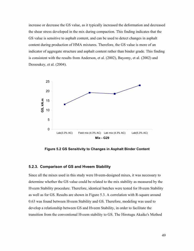
49
increase or decrease the GS value, as it typically increased the deformation and decreased
the shear stress developed in the mix during compaction. This finding indicates that the
GS value is sensitive to asphalt content, and can be used to detect changes in asphalt
content during production of HMA mixtures. Therefore, the GS value is more of an
indicator of aggregate structure and asphalt content rather than binder grade. This finding
is consistent with the results from Anderson, et al. (2002), Bayomy, et al. (2002) and
Dessoukey, et al. (2004).
0
5
10
15
20
25
Lab(3.3% AC) Field mix (4.3% AC) Lab mix (4.3% AC) Lab(5.3% AC)
Mix - G29
GS,
kN
.m
Figure 5.2 GS Sensitivity to Changes in Asphalt Binder Content
5.2.3. Comparison of GS and Hveem Stability
Since all the mixes used in this study were Hveem-designed mixes, it was necessary to
determine whether the GS value could be related to the mix stability as measured by the
Hveem Stability procedure. Therefore, identical batches were tested for Hveem Stability
as well as for GS. Results are shown in Figure 5.3. A correlation with R-square around
0.63 was found between Hveem Stability and GS. Therefore, modeling was used to
develop a relationship between GS and Hveem Stability, in order to facilitate the
transition from the conventional Hveem stability to GS. The Hirotugu Akaike's Method

50
(AIC) in the statistical software package SAS was used to choose the best prediction
model (Ott and Longnecker 2001 ). This model is shown in Equation 5.1.
βα += HSGS . (5.1)
where,
HS is the predicted Hveem Stability,
α, β are regression parameters and were found to be equal to 0.9579 and -18.988
respectively,
and R2 = 0.6386.
0
5
10
15
20
25
30
30 35 40 45 50
Hveem Stability
Gyr
ator
y St
abili
ty, k
N.m
GS = 0.9579 (HS) - 18.988R2 = 0.6386
Figure 5.3 Relation between Hveem Stability and Gyratory Stability
For the tested mixes, a range of GS design threshold values were suggested as shown in
Table 5.1, based on the Hveem stability limits used in the State of Idaho. The suggested
GS limiting values could be different for Superpave-designed mixes.

51
Table 5.1 Proposed Design Values of GS for Hveem-Designed Mixes Mix Class ITD General Specifications
Traffic Category Hveem Stability
GS, kN.m
I Heavy
(> 106 ESALs) > 37 >15
II Medium
(104 – 106 ESALs) > 35 >12
III Light
(< 104 ESALs) > 30 > 5
5.2.4. Comparison of GS with Permanent Deformation in APA
The Asphalt Pavement Analyzer (APA), which is the new generation of the Georgia
Loaded-Wheel Tester, was developed to evaluate the HMA resistance to permanent
deformation (Choubane, et al. 2000; Martin and Park 2003; and Bhasin, et al. 2004). The
APA has the capability to test both rectangular and cylindrical specimens. Permanent
deformation tendencies can be determined on three beam specimens, six cylindrical
specimens, or a combination of both. The test temperature depends on the upper
temperature range of the binder grade (i.e., 76 °C for PG 76-28 and PG 76-34). Sixteen of
the mixtures used in this study were tested using the APA. Theses mixes were compacted
to achieve 4% final air voids and to a fixed height of 150 ± 5 mm. Each mix had three
duplicates.

52
R2 = 0.1631
0
1
2
3
4
5
6
15 17 19 21 23 25 27 29 31
GS, kN.m
APA
Rut
-Dep
th, m
m
Figure 5.4 Relation Between APA Rut-Depth and GS
The GS value was compared to the APA test results as shown in Figure 5.4. The results
show that there is no relationship between the APA permanent deformation and GS. This
result is attributed to the fact that the APA test is conducted at different temperatures,
according to the upper temperature of the PG grade, while GS is measured at the standard
compaction temperature of the binder, around 149 °C. Therefore, it was decided to
investigate the relationship between APA results and GS for each group of asphalt mixes
with the same high temperature grade separately. Figure 5.5-a shows that a very good
correlation exists between APA and GS for PG 58 – 28 and PG 58 – 34 binder grades.
However, this was not the case for the PG 64 – 28 and PG 64 – 34 binders, as shown in
Figure 5.5-b.

53
0
5
10
15
20
25
30
G19 G23 G31 G25 G28 G27 G29-L
a) Mix Groups with PG 58-28 or PG 58-34
GS,
kN
.m
0
0.5
1
1.5
2
2.5
3
3.5
4
APA
Rut
Dep
th, m
m
GS, kN.mRut Depth, mm
0
5
10
15
20
25
30
G26 G22 G20 G32
b) Mix Groups with PG 64-28 or PG 64-34
GS,
kN
.m
0
0.5
1
1.5
2
2.5
3
APA
Rut
-Dep
th, m
m
GS, kN.mRut Depth, mm
Figure 5.5 APA Test Results
5.2.5. Influence of Aggregate Shape Characteristics on GS
Previous analysis of GS development indicated that the GS value is more dependent on
the interlocking mechanism of the aggregate-asphalt matrix. Therefore aggregate
characteristics are expected to affect the GS value. The Aggregate Imaging System
(AIMS) was used to measure three aggregate properties. These are surface texture,
angularity and sphericity.
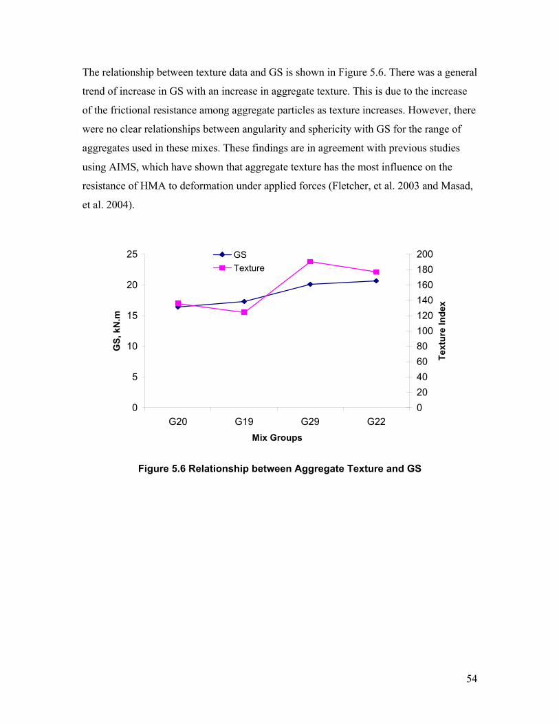
54
The relationship between texture data and GS is shown in Figure 5.6. There was a general
trend of increase in GS with an increase in aggregate texture. This is due to the increase
of the frictional resistance among aggregate particles as texture increases. However, there
were no clear relationships between angularity and sphericity with GS for the range of
aggregates used in these mixes. These findings are in agreement with previous studies
using AIMS, which have shown that aggregate texture has the most influence on the
resistance of HMA to deformation under applied forces (Fletcher, et al. 2003 and Masad,
et al. 2004).
0
5
10
15
20
25
G20 G19 G29 G22Mix Groups
GS,
kN
.m
020406080100120140160180200
Text
ure
Inde
x
GSTexture
Figure 5.6 Relationship between Aggregate Texture and GS

55
5.2.6. Summary
Based on the results of this study, it is concluded that the Gyratory Stability (GS) could
be used as a first screener to distinguish among mixes for mix design acceptance,
especially to decide on the acceptance of the mix aggregate structure. The following
conclusions and observations were also made:
• The GS value correlated well with the Hveem Stability of Hveem-designed mixes.
Results, however, showed a wide variation in GS values for mixes that had the
same Hveem Stability. This may indicate that GS is more sensitive to changes in
mix design parameters than Hveem Stability. Three tiers of GS limits (5, 12 and
15) are suggested to classify HMA mixtures, based on their stability.
• Results of the APA rut testing did not correlate with the GS value of these mixes.
The main reason is believed to be that the current APA testing procedure allows
for testing the mix at different temperatures based on its high temperature grade;
while, GS is determined at the standard compaction temperature of 149 °C. A
better correlation between GS and permanent deformation in APA was obtained
for mixes that had the same PG grade and were tested at the same temperature in
the APA.
• Image analysis indicated that aggregate texture correlated with the GS value.
There was no clear relationship between angularity and sphericity with GS, for
the range of aggregates used in this study.

This is a Blank Page

56
6. EVALUATION OF HVEEM DESIGNED HMA FRACTURE TOUGHNESS USING THE JC PARAMETER
6.1. INTRODUCTION
The Superpave method of mix design has been used by pavement engineers for more than
a decade, yet a fracture-based mix design criteria has not been developed to ensure that
the designed Superpave mixes will not show cracking and fracture before the end of the
design life of the mix or pavement. Superpave ensures low-rutting and low-temperature
cracking of a designed mix using Performance Grade (PG) binders; however, there are no
reliable design criteria and/or test methods that will ensure that the designed mix will not
show cracking and fracture. There is a need for the development and evaluation of a test
method and design criteria to ensure Superpave mix’s resistance to fracture and cracking
(Mull, et al. 2002). In this study, a fracture based parameter, Jc determined in a Semi-
Circular Notched Bending Fracture (SCNBF) test is evaluated for HMA mix resistance to
fracture and cracking.
The use of the fracture-based concept in asphalt mix design has been investigated for
several decades. Little and Mahboub (1985) used the Jc value to compare the fracture
resistance of asphalt mixes prepared with and without plasticized sulfur binder. Dongre,
et al. (1989) evaluated the fracture resistance of asphalt mixes at low temperatures, using
bending beam specimens. Their study showed that Jc is a promising fracture
characterization parameter for asphalt mixes at low temperatures. Furthermore, their
study concluded that Jc is sensitive to asphalt mix stiffness and it is a better fracture
characterization parameter than the plane strain critical stress intensity factor (KIC).
Abdulshafi, et al. (1985) used V-shaped notched circular samples to determine Jc for
different asphalt mixes and used the Jc value to predict the fatigue life of asphalt mixes.
Bhurke, et al. (1997) studied polymer modified asphalt concrete using the Jc fracture
resistance approach, employing three point bending beam specimens. Their study used
AC-5 asphalt as a base and polymers, such as styrene-butadiene-styrene, and styrene-

57
butadiene rubber as modifiers. They concluded that the three-point bending beam test is
repeatable, and test results are sensitive to material differences due to polymer
modification.
Recently, several studies were initiated to utilize the gyratory compacted samples in a
three point bending test. Ven, et al. (1997), Molennar, et al. (2002), and Li, et al. (2004)
adopted the semi-circular bending test set-up, using the Superpave Gyratory Compactor
(SGC) samples, to determine tensile strength of asphalt mixtures, in an effort to replace
the indirect tensile test. They, however, used un-notched samples and did not focus on
fracture resistance parameters. In rock mechanics, Lim, et al. (1994) used a semi-circular
notched specimen in a bending test to evaluate the fracture properties of natural rocks by
determining the KIC parameter. Mull, et al. (2002) adopted this semi-circular bending test
with notched specimens to measure fracture toughness properties of asphalt mixtures.
They determined Jc, to evaluate the fracture resistance of chemical crumb rubber asphalt
(CMCRA) mixes. In that study, the three binders used were (i) a base binder produced
from air-blown asphalt with no catalyst, (ii) the base binder modified using plain crumb
rubber asphalt (CRA), and (iii) the based binder chemically modified using crumb rubber
asphalt (CMCRA). Their study showed that the fracture resistance, Jc, value of the
CMCRA is twice the Jc value of the CRA mix; the base mix had the lowest value of Jc.
These researchers also compared their laboratory results to the micromechanical
damage/fracture seen under a scanning electron microscope.
Huang, et al. (2004) used the Semi-Circular Notched Bending Fracture (SCNBF) test to
study the fracture properties of various reclaimed asphalt pavement (RAP) mixes. Their
analysis showed that the fracture resistance measured by the Jc increases with the
increase of RAP content in the mix to a certain extent, after which, the fracture resistance
decreases significantly. Mohammed, et al. (2004) used the SCNBF test geometry to study
the effect of recycled polymer modified asphalt cement (RPMAC) content on the fracture
resistance, the Jc. These researchers found that as the percent of RPMAC increases, the
stiffness and maximum sustained load also increase, with a slight decrease in the

58
deflection at maximum load. Their study suggests that the semi-circular fracture test used
in conjunction with Jc analysis can be a useful mix design tool.
Very recently, Mull, et al. (2004) extended the concept of the SCNBF test to study
fatigue crack propagation of asphalt mixes. They found that the SCNBF test geometry
provides a suitable geometry for fatigue crack propagation analysis of asphalt mixes. In
addition, they showed that the fatigue lifetime of CMCRA mixes are higher than that of
unmodified crumb rubber mixtures. The results of the fatigue study on the crumb rubber
modified mixtures have confirmed the static Jc results generated earlier by Mull, et al.
(2002). Both studies found SCNBF to be a reliable test asphalt mixtures evaluation.
In addition, studies have shown that a relationship between KIC and Jc exists in metals.
Landes, et al. (1984) has related KIC to Jc using the following equation:
ν 22
1.
−=
EJK CIC (6.1)
where,
E= elastic Modulus, and
ν= Poisson Ratio.
McCabe, et al. (2005) has used a modified equation to determine an equivalent stress
intensity factor defined as KJC (Equation 6.2). It has been demonstrated that to determine
KJC, specimens can be 1/40th the size required for KIC validity by ASTM Standard E 399,
and still maintain sufficient control of constraint.
JEK cJC .= (6.2)
The aforementioned literature studies reveal that Jc can be determined by various
methods and used as an indicator of the asphalt material’s fracture resistance to cracking.
Therefore, the present study has adopted the Jc parameter for evaluating HMA resistance

59
to fracture and crack propagation. It can be noted that Jc is chosen over the stress
intensity factor, KIC in this study. The KIC value represents the linear elastic energy
release around a crack, where as Jc represents the non-linear elastic energy release around
a crack. It is shown later that an asphalt concrete follows the nonlinear stress-strain
behavior. Therefore, the adoption of Jc over KIC in the study of fracture behavior of
asphalt concrete is appropriate. In addition, the KIC is dependent on the sample geometry,
and the functional form of KIC for semi-circular shape is yet unknown, to the best of this
researcher’s knowledge. To this end, the Semi-Circular Notched Bending Fracture
(SCNBF) test is adopted for Jc evaluation in this study. The goal is to evaluate the
fracture resistance parameter, Jc, of a wide variety of field mixes used by the Idaho
Transportation Department (ITD) and to identify its sensitivity to HMA properties.
6.2. FRACTURE PARAMETER, JC
The fracture parameter, Jc, used in this study is based on the study conducted by Rice
(1968). The Jc is defined as a path independent integration of strain energy density,
traction, and displacement along an arbitrary contour path around the crack, as shown in
Figure 6.1, and can be quantified using the following equation:
dsxuTWdyJ
ΓΓc ∂
∂∫∫ −= (6.3)
where,
Γ = any path surrounding the crack tip,
x,y = rectangular coordinates normal to the crack front,
ds = increment along contour Γ,
T = stress vector acting on the contour,
u = displacement vector, and
W = the strain energy density = εσ ijijd∫ .

60
Y
XO
I
dsn
crack
Figure 6.1 Line Contour Surrounding Crack Tip
Rice (1968) also presented an alternative and equivalent definition for Jc, based on the
pseudopotential energy difference between two identically loaded bodies possessing
slightly different crack lengths. A simplified form of Equation (6.1) is given below:
⎟⎠⎞
⎜⎝⎛
∂∂
=bU
aJ c (6.4)
where,
U is the strain energy to failure, which is the area underneath the load-deformation
curve up to the peak load,
b is the specimen thickness, and
a is the notch depth.
Equation (6.4) was used to calculate Jc in this study. As a preliminary step to calculating
Jc, the load versus deformation diagram was plotted using laboratory data. Next, the area
under the load-deformation curve, defined as the strain energy U, was determined and
divided by the sample thickness. A total of three specimens of different notch depths
were used. Next, strain energy per unit depth for all three samples were plotted as a
function of notch depth. The slope of the best-fit line was determined as the critical
fracture resistance parameter, the Jc, as shown in Figure 6.2.

61
Mix Class II (G20-L / PG 76-28)Sample 1
y = -0.6924x + 29.474R2 = 0.9958
0
5
10
15
20
25
0 10 20 30 40 50
Notch, mm
Ener
gy/th
ickn
ess,
N.m
m/m
m
Mix Class II (G20-L / PG 76-28)Sample 1
0
50
100
150
200
250
0 0.02 0.04 0.06 0.08 0.1 0.12 0.14
Deformation, mm
Load
, N
38 mm Notch26 mm Nptch15 mm Notch
Class Mix I (G 24-L)Sample 1
y = -1.141x + 46.632R2 = 0.8775
0
5
10
15
20
25
30
35
0 10 20 30 40
Notch, in
Ener
gy/th
ickn
ess,
N.
mm
/mm
Mix Class I (G24-L)Sample 1
0
500
1000
1500
2000
2500
0 0.5 1 1.5 2 2.5 3 3.5
Deformation, mm
Load
, N38 mm Notch27 mm Notch15 mm Notch
Mix Class I (G18-L)Sample1
y = -0.5338x + 20.145R2 = 0.9075
0
2
4
6
8
10
12
14
0 10 20 30 40 50
Notch, mm
Ener
gy/th
ickn
ess,
N.
mm
/mm
Mix Class I (G18-L)Sample 1
0100200300400500600700800900
0 0.5 1 1.5 2 2.5 3
Deformation, mm
Load
, N
38 mm Notch26 mm Notch15 mm Notch
b) Mix G20-L (Class II with PG 76-28)
c) Mix G18-L (Class I with PG 64-34)
a) Mix G24-L (Class I with PG 76-28)
Figure 6.2 Jc Determination for three Different Asphalt Mixtures

62
6.3. PREPARATION OF SPECIMENS AND TEST SETUP
The HMA samples were compacted using a Superpave Gyratory Compactor (SGC) to
achieve final air voids of 4±1%. Each sample was sliced into 4-quarter specimens. These
quarter specimens were tested to determine Jc. One of the quarters was left un-notched to
determine the stiffness, which was used in the development of the Finite Element
Analysis (FEA) model. The other three quarters were notched to various notch depths.
Notches were in the range from 12.5 mm (½ in) to 38 mm (1 ½ in) in depth and about 2
mm in width, as shown in Figure 6.2. Three replicates were prepared for each mix. All
specimens had 150 mm diameter and 110±5 mm height, which is the standard size of a
Superpave Gyratory compacted specimen.
Figure 6.3 illustrates the test configuration of the Semi-Circular Notched Bending
Fracture (SCNBF) test. In the fracture bending test, the spacing between the two roller
supports is 122 mm. A ramp load with a constant vertical deformation rate of 0.5
mm/minute was applied until fracture occurred. The test was conducted at a room
temperature of approximately 25±1°C.
Figure 6.3 Semi-Circular Notched Specimens Sliced from a Standard Gyratory Compacted HMA Sample

63
Figure 6.4 Semi-Circular Notched Bending Fracture Test Setup
6.4. ANALYSIS OF RESULTS
6.4.1. Jc Calculations
The value of Jc was determined for all tested mixtures given in the Appendices, in
accordance with the concepts presented previously. For each sample, the applied load
versus the vertical deformation was plotted. The strain energy U, which is equal to the
area underneath the load-deformation curve up to the peak load, was determined. After
determining the strain energy, the ratio of the strain energy to the specimen thickness,
U/b, for each specimen was plotted against the notch depth, a. The value of Jc was
obtained from the slope of the U/b versus a best straight line fit. As indicated earlier, at
least three data points are needed to develop such a line fit, and therefore, three
specimens with different notch depth were tested for the Jc calculation. For each notch
depth, three replicate specimens were used to evaluate test repeatability.
The laboratory produced mixes in Figure 6.2 and 6.5 were designated as G24-L (Class I,
PG 76-28), G20-L (Class II, PG 76-28) and G18-L (Class I, PG 64-34). The difference
between the first two mix classes is that one mix is finer than the other (courser grade
aggregate). The difference between the first mix and the third mix class is in PG grade.
The test results are shown in Figure 6.2 and 6.4. It can be seen from Figure 6.4 that the
fracture resistance parameter Jc for the G24-L mix is higher than that of the G18-L mix.

64
Comparing G24-L and G20-L, it is seen that the Jc for the courser grade is lower than that
for the finer grade mix with the identical PG.
0.00.20.40.60.81.01.21.4
Mix Group
J c, k
J/m
2
Average 0.55 0.62 1.20
Variance 0.0032 0.0100 0.0252
G18-L G20-L G24-L
Figure 6.5 Jc Determination for three Different Asphalt Mixtures
These comparisons show that Jc is affected by the change in mixture composition, both in
terms of aggregate gradation and asphalt type. Therefore, it may be useful to find the
relationships between HMA properties and Jc. The values of Jc for the mixtures studied
herein range from 0.53 to1.2 kJ/m2, which is within the range of Jc values reported
previously in other studies (Mull, et al. 2002), as shown in Figure 6.6.
0.41
0.91
0.550.62
0.70
1.20
0.540.65
1.23
0.0
0.2
0.4
0.6
0.8
1.0
1.2
1.4
G2 G5 G18 G20 G21 G24 Control CRA CMCRMix
J c, k
J/m
2
Tested
Reported (Mull et al. 2002)
Figure 6.6 Comparison of Jc between ITD Mixes and Reported Mixes

65
6.4.2. Finite Element Analysis
To calculate the elastic modulus, an approximation was made by assuming that the
asphalt mixture was a homogeneous and isotropic material. Finite Element Analysis
(FEA) software, ALGOR version 15.0, was used in this study to calculate the elastic
modulus E of the asphalt mixtures. In FEA, a 3-D idealization model with quadratic
elements was used. Quadratic elements are more suitable than the tetrahedral elements in
defining the geometrically isotropic characteristics. Also, the linear variation of stress-
strain over the entire area of a quadratic element makes the quadratic elements more
appropriate for studying bending characteristics. The boundary conditions for the FE
model were set to restrain the specimen vertically at 0.1 and 0.9 the diameter, with one
side restrained horizontally to avoid movement of the whole model. The load was
statically increased. A few changes were made, especially at the loading and support
points. For example, the number of the loading and restrained nodes was increased to
avoid local failure, especially by compressive stresses.
The simplest way to characterize the behavior of an asphalt mix under a given load is to
consider it as a homogeneous half-space material. A half-space has an infinitely large
area and an infinite depth with a top plane on which the loads are applied. Commonly, the
stresses, strains and deflections are calculated using the Burmister (1943) theory, which is
based on elastic half-space. Further, the HMA is assumed to be isotropic, linearly elastic
with an elastic modulus, weightless, and with uniform and clean surfaces (Huang 2004).
Running the simulation in ALGOR, as shown in Figure 6.7, we observed that the
maximum tensile stress occurs in the bottom of the specimen as expected. Employing
Equation (6.3) with the value of δz, as measured from the experiments, the value for the
elastic modulus E of the mixes listed in the Appendices were back calculated.

66
Figure 6.7 Contour of Tensile Stress from the FE Model
The research team adopted Finite Element Method (FEM) due to the lack of fracture tests
and parameters at their disposal to evaluate the Jc parameter. The research team
acknowledges that FEA is not accurate in describing the behavior of HMA, due to the
basic assumptions in FEA: that HMA is isotropic, linearly elastic with an elastic
modulus, weightless, has uniform and clean surfaces, and that no separation of elements
may occur (no fracture). The calculated E values were used to evaluate Jc.
6.4.3. Effect of Elastic Modulus on Jc
There is no closed-form solution for determining the tensile stress and deformation of a
Semi-Circular Notched Specimen loaded in a three-point bending setup as in the
configuration described here. Therefore, Finite Element Analysis (FEA), as well as
statistical analysis, is employed to develop Equations (6.5) and (6.6) for determining the
tensile stresses at the bottom of a sample, and vertical deformation of an un-cracked
semi-circular specimen. These stress and deformation values are used to calculate elastic
modulus:
WDF
t888.4
=σ (6.5)

67
WEF
z26.2
=δ (6.6)
where,
σt = Tensile stress at the bottom of the sample,
δz= Deformation in the vertical direction,
F= Applied force,
W= Width of the specimen,
D= Diameter of the sample, and
E= Elastic modulus.
The aforementioned approach was demonstrated by Ven de Ven, et al. (1997). In the
present study, the un-notched specimen (un-cracked semi-circle) shows linear elastic –
plastic and viscoelastic response. Nevertheless, the first portion of the curve appears to be
linear where the elastic modulus can be obtained (see Figure 6.2).
The relationship between the elastic modulus (E) and fracture resistance (Jc) for all the
mixtures under consideration is shown in Figure 6.8. The results show that an increase in
the E value is associated with high toughness. This is because an increase in the stiffness,
or E, will lead to an increase in the strain energy U required to fracture the sample.
Further examination of the data in Figure 6.8 reveals that, for the three classes of the ITD
mixtures, Class III (lowest stability) has lower stiffness and lower Jc when compared to
Class I (highest stability). Some of the Class I mixtures, such as G24-L with PG76-28,
possess the highest Jc and the highest stiffness. Class II mixtures, however, had higher
values of Jc than that of Class III with some of the mixes in Class II overlapping with
Class I. Overall, it was observed that Jc and E results reflect that Hveem-designed mixes
with higher stabilities (as indicated by the mix class) may also have higher stiffness and
higher resistance to fracture as measured by the Jc parameter.

68
0
5000
10000
15000
20000
25000
30000
35000
40000
45000
50000
0 0.2 0.4 0.6 0.8 1 1.2Jc, kJ/m2
E, M
Pa Class I
Class II
Class III
Figure 6.8 Relationships of Jc and the Calculated Elastic Modulus
Using the estimated E from the developed FEA model and the Jc for the tested mixes, KJC
was calculated using Equation (6.2) and compared to Jc as shown in Figure 6.9. Results
have shown that KJC followed the same trend as Jc for the tested mixes. In addition,
Dongre, et al. (1989) has reported a range of 3.62 – 5.34 MPa.m1/2 for KIC at 25°C testing
temperature for tested asphalt mixes. KJC of the tested mixes in this study has a range of
1.42 – 7.43 MPa.m1/2 at the same temperature (Figure 6.10).
0.00.20.40.60.81.01.21.4
58-28
64-28 G1 G3 G6
G10 G18 G21 G24 G26 G27
G29(-1
%)G29 G31 G33 G35
Mixes
J c, K
J/m
2
012345678
K Jc,
MPa
.m0.
5Jc KJc
Figure 6.9 KJC and JC Results

69
5.40
3.922.96
3.92
6.39
7.43
1.42
4.403.62
5.48
4.42
0
1
2
3
4
5
6
7
8
G6 G8 G10 G21 G24 G24(-1%)
G27 G33 Mix 2 Mix 12 Mix 13
Mix
MPa
.m1/
2
KJc
Reported KIc (Dongre et al1989)
Figure 6.10 KJC and Reported KIC
6.4.4. Effect of Aggregate Characteristics on Jc
The analysis of Jc as it varies with mix class may reflect changes in aggregate gradation,
but does not reflect its variation in aggregate shape and texture properties. Therefore, an
investigation of the effect of aggregate surface characteristics was conducted. The
Aggregate Imaging System (AIMS) developed by Masad (2003) was used to determine
aggregate shape and surface properties. The AIMS at Texas A&M University testing
laboratory was used to measure three aggregate properties as recommended by Masad, et
al. (2004). These included surface texture, angularity, and sphericity. Texture is analyzed
using the wavelet transform, which captures the changes of texture on gray scale images.
The wavelet transform gives a higher texture index for particles with rougher surfaces.
Aggregate angularity is measured using the gradient method. In this method, the changes
in the gradients on the boundary of a two-dimensional projection of a particle are
calculated. The angularity index, calculated using the gradient method, increases with an
increase in aggregate angularity. Shape is quantified using the sphericity index, which is
equal to one for particles that have equal dimensions, and decreases as particles become
more flat and elongated (Masad 2003 and Fletcher, et al 2003).

70
The relation between Jc and the aggregate characteristics (texture, sphericity, and
aggregate shape or L/S ratio) measured by AIMS was investigated. Here, L is the length
and S is shortest dimension of an aggregate. Initial findings showed that:
• The Jc increased for mixes that contained aggregates with rough surface texture.
This is due to the fact that rougher aggregate surfaces have higher bond strength
between the aggregates and the binder, thus they display a higher fracture
resistance (Figure 6.11-a).
• The Jc increased for mixes that have more angular aggregates. The angular
aggregates resisted crack propagation and made the failure path longer, which
resulted in higher fracture toughness. (Figure 6.11-b).
• Aggregate flatness and elongation, as indicated by an L/S ratio of > 3 and > 5, has
been shown to have an adverse effect on mix performance. Results show that Jc
decreases for mixes that have a higher percentage of aggregates with L/S > 3 and
> 5. This indicates that a mix with a higher percentage of flat and elongated
aggregates tends to be weak and more easily fractured than a mix with a lower
percentage (Figure 6.11-c) of flat and elongated particles.

71
Figure 6.11 Variation of Jc with Aggregate Shape and Texture Characteristics
0.00.10.20.30.40.50.60.70.8
G19 G20 G29 G22
Mix Groupa) Aggregate Surface Texture
J c, k
J/m
2
0
50
100
150
200
Text
ure
Jc
Texture
0.00.10.20.30.40.50.60.70.8
G19 G20 G29 G22
Mix Groupb) Aggregate Angularity
J c, k
J/m
2
050010001500200025003000350040004500
Ang
ular
ity -
Gra
dien
t
Jc
Angularity - Grad. (f ine)
Angularity - Grad. (coarse)
0.00.10.20.30.40.50.60.70.8
G19 G20 G29 G22
Mix Groupc) Aggregate Flatness and Elongation
J c, k
J/m
2
0
10
20
30
40
50
60
% A
ggre
gate
Par
ticle
s
Jc
% L/S >3
% L/S >5

72
6.5. EFFECTS OF ASPHALT CONTENT AND BINDER GRADE
Figure 6.12 shows the Jc values of mixes with identical aggregate gradation but different
asphalt binder contents. The value of Jc was found to be sensitive to the variation in the
asphalt binder content. As the percentage of asphalt content increases, the value of Jc
increases. As expected, the Jc for the field mix is very close to that prepared in the
laboratory with the same asphalt binder content. The increase in the binder content
increases the cohesion behavior of the mixture, which has resulted in an increase in the
fracture resistance (Jc ) potential of an HMA mix.
The effect of binder grade on the Jc was also studied, based on four mixtures from Class
II shown with their results in Figure 6.13. No trend in the data can be observed from
Figure 6.13 in this study. It is possible that the dependency of Jc on asphalt binder grade
is complex.
0.00
0.10
0.20
0.30
0.40
0.50
0.60
0.70
Field mix Lab(-1% AC) Lab mix (4.3 AC%) Lab(+1% AC)
Mix Group: G29
J c, k
J/m
2
Figure 6.12 Variation of Jc with Asphalt Binder Content

73
0.00
0.10
0.20
0.30
0.40
0.50
0.60
0.70
0.80
PG 58-28 PG 58-34 PG 64-28 PG 76-28Asphalt Binder Grade
Mix Group: G20
J c, k
J/m
2
Figure 6.13 Sensitivity of Jc to Asphalt Binder Grade
6.6. SUMMARY
As a summary based on the results presented, the following observations are made:
• The Jc parameter measured by the semi-circular notched bending fracture
(SCBNF) test can represent HMA resistance to fracture. The SCBNF test is
simple and quick to perform, and can be implemented at the mix design stage of
HMA design.
• Finite Element Analysis was used to model the SCBNF test configuration. FEA
results were used to calculate the mixture elastic modulus. The elastic modulus
was correlated to the Jc. It is shown that Jc increases with the increase in modulus
values of HMA. It is postulated that Hveem mixes with higher stabilities have
higher stiffness and therefore, higher resistance to fracture, as measured by the Jc
parameter.

74
• Results have shown that KJC, which is equivalent to KIC, follows the same trend as
Jc for the tested mixes and fall in the range of reported KIC.
• The Jc parameter was found to be sensitive to changes in the mix aggregate
gradations and to the aggregate shape and surface texture properties, as measured
by the Aggregate Imaging System (AIMS). Mixes with finer aggregate gradations
showed higher resistance to fracture compared to the mixes with coarser
aggregate gradations. Mixes with rougher aggregate texture and more angular
particles showed higher Jc values. Mixes that had high percentages of flattened
and elongated aggregates showed lower Jc values.
• The Jc parameter was found to be sensitive to variations in the asphalt binder
content. In this study, as the binder content increased, the value of Jc increased.
• In this study, no clear trend was found to demonstrate Jc sensitivity to variations
in binder grades.
• Overall, this study concludes that Jc, determined in a SCNBF test, can be used to
assess an HMA mixture’s propensity to fracture during the design stage.

This is a Blank Page

75
7. EVALUATION OF IDAHO SUPERPAVE MIXES
7.1. INTRODUCTION
The research outcomes of the Strategic Highway Research Program (SHRP) included
state-of-the-art methods to design the Hot-Mix Asphalt (HMA) based on performance.
However, and for practical implementation of SHRP products, the main design criterion
in the current Superpave system is based only on volumetric analysis. There is a need to
develop simple, practical and reliable methods and procedures that can be incorporated
into the design criteria of Superpave. Research efforts since the release of Superpave in
1992 have continued to address this issue. A few test procedures and new performance
indicators have been developed.
Under the NCHRP Project 9-19 a simple performance test (SPT) setup was developed
that included Dynamic Modulus, Flow Number and Flow Time tests. Recent Studies
(Bhasin, et al.; Tandon, et al.; Zborowski, et al. 2004; and Bahia, et al. 2005) have
concluded that SPT can be used to indicate the performance of HMA. However, mix
performance evaluation methods such as SPT that were developed under the SHRP plans
were found to be highly sophisticated and time consuming for the mix design stage.
As a final stage of this study, the research team investigated the utilization of Gyratory
Stability (GS) and the Fracture Toughness Parameter (Jc) as simple and practical test
methods that can be used in conjunction with the current Superpave mix design
procedure. Hence, mix performance can be assessed and incorporated into the design
criteria during the mix design stage.

76
7.2. EXPERIMENT MEASUREMENT AND ANALYSIS
7.2.1. Selected Mixes
ITD has recently begun the implementation of Superpave mix design. Three trial projects
were underway when this study was completed. Two different mixes were procured from
two projects. These two mixes have different aggregate types and gradation (Figure 7.1.)
Figure 7.1 Tested Superpave Mixes
To achieve the goals and objectives of the final stage of this study, an experimental mix
matrix was prepared to evaluate these mixes and the effect of binder content and grade on
the performance, as shown in Table 7.1.
Table 7.1 Idaho Superpave Mixes Matrix
-1.0% -0.5% Optimum +0.5% +1%
1 64-34 √ 5.5% √ √
64-22 √
64-28 √ √ 5.9% √ √
64-34 √
Mix PG
AC%
2
77
7.2.2. Sample Preparation
For the purpose of investigating the performance of these mixes, their raw materials were
provided by ITD. All specimens were mixed and compacted under controlled lab
conditions. Specimens used to determine the Gyratory Stability and Jc were compacted
using the Servopac Gyratory Compactor to a number of gyrations to produce specimens
with 4% air voids. For the optimum asphalt content for both mixes, the number of
gyration coincided as expected with their set N-design.
Specimens used in the Dynamic Modulus and Flow Number tests were compacted to
achieve seven inch height specimens with a total of 9% air voids. Then the specimens
were cored and sawed to obtain specimens with a four inch diameter, six inch height and
7% air voids.
7.2.3. Gyratory Stability (GS) and Asphalt Pavement Analyzer (APA) Test
See Chapter 5 for test setup and test procedures.
7.2.4. Fracture Toughness (Jc)
See Chapter 6 for test setup and test procedures.
7.2.5. Dynamic Modulus Test
The Dynamic Modulus (|E*|) is defined as the absolute value of the Complex Modulus
(E*), which is the stress-to-strain relationship for a linear viscoelastic material.
Mathematically, the Dynamic Modulus is equal to the maximum stress (σo) divided by
the maximum recoverable strain (εo) as in shown in Equation 7.1.
o
oEεσ
=* (7.1)
78
The Dynamic modulus Test (AASHTO TP 62-03) consists of applying a uniaxial
sinusoidal (haversine) compressive stress to an unconfined HMA cylindrical test
specimen as shown in Figure 7.2 and measuring the corresponding strain using two to
three LVDTs mounted on the middle of the specimen.
Figure 7.2 Haversine Loading for the E* Test (after Witczak 2002)
The Dynamic Modulus Test protocol AASHTO TP 62-03 indicates that the test shall be
conducted under a series of temperatures (14o F, 40 o F, 70 o F, 100 o F and 130 o F) and
loading frequencies (0.1 Hz, 0.5 Hz, 1 Hz, 5 Hz, 10 Hz and 25 Hz) at each temperature.
The (E*/sin δ) parameter at a loading frequency of 5 Hz at temperatures of 100 o F and
130° F was used as a permanent deformation (rutting) indicator and where δ represented
the time lag between the application of load and the material response (Figure 7.2). In
addition, the (E*.sin δ) parameter at a loading frequency of 5 Hz at temperatures of 40 o F
and 70° F was used as a fracture resistance indicator for the tested mixes. Both
parameters and conditions are recommended by Witczak, et al. (2002).
7.2.6. Flow Number Test
The Flow Number (FN) is defined as the number of load repetitions at which shear
deformation, under constant volume, starts (Figure 7.3). Witczak, et al. (2002) concluded
in their study that this fundamental engineering property of HMA can also be used as a
performance indicator for permanent deformation (rutting). The Flow Number test is
conducted using a loading cycle of 1.0 second in duration, which consists of a 0.1 second

79
haversine load, followed by a 0.9 second rest at a testing temperature of 130° F. This test
utilized the same specimens used for the Dynamic Modulus Test. Both tests (the
Dynamic Modulus and Flow Number) were conducted at Washington State University
labs.
Figure 7.3 Typical Repeated Load Test Response and Flow Number (after Banaquist 2003)
7.3. ANALYSIS OF RESULTS
7.3.1. Gyratory Stability
The GS values were calculated for both mixes with different asphalt contents, and as per
Superpave Mix Design, these mixes were expected to perform best at the optimum
asphalt content, at which the air voids of the compacted specimen at N-design is four
percent. As shown in Figure 7.4 both mixes yielded the highest GS, as expected, at
optimum asphalt content. In addition, when comparing the two mixes’ GS values, Mix 2

80
yielded higher GS values, which leads us to the conclusion that Mix 2 may perform better
than Mix 1.
0
5
10
15
20
25
4 4.5 5 5.5 6 6.5 7 7.5
AC%
GS
, kN.
mMix 1Mix 2
Figure 7.4 Superpave Mix GS Results for Different Asphalt Contents
The GS sensitivity to binder type (PG grade) was evaluated for Mix 2 (Figure 7.5). As
expected, the results showed that GS is not very sensitive to the changes in binder grade.
These findings matched the results for Hveem-designed mixes (Chapter 5). This can be
explained by the fact that at compacting temperatures, asphalt binder is in a liquid state
and the difference in grade does not influence the performance of the mix.
0
5
10
15
20
25
PG 64-22 PG 64-28 (Opt AC%) PG 64-34
Binder
GS,
kN
.m
Figure 7.5 Sensitivity of GS to Different PGs (Mix 2)

81
Then GS results were compared to the APA test results. Figure 7.6 shows that a very
good correlation between GS and permanent deformation resulted from APA (R2 = 0.58).
These results vary from the results for the Hveem mixes (Chapter 5). The correlation is
attributed to the fact that the APA test is conducted at different temperatures, according
to the upper temperature of the PG grade; and since both mixes have the same upper
temperature of the PG grade (64 °C) a correlation should exist between the two
parameters. This relation shows that the higher the GS, the lower the permanent
deformation predicted by APA will be.
R2 = 0.58
0
5
10
15
20
25
0 1 2 3 4 5 6 7 8 9 10
APA, mm
GS,
kN.
m
Figure 7.6 Relationship of GS versus APA Test
As suggested by Witczak, et al. (2002) E*/sin δ at the 130 o F or at the 100° F parameter
should be used as a rutting indicator for asphalt mixes, because the higher the value of
this parameter at a given temperature, the better resistance to rutting the mix exhibits. The
GS was compared to E*/sin δ at both temperatures. Figure 7.7 shows that a very good
relationship exists between GS and E*/sin δ at 130° F with an R2 equal to 0.76; and also
between GS and E*/sin δ at 100° F with an R2 equal to 0.65.

82
R2 = 0.76
0
5
10
15
20
25
0 100 200 300 400 500 600 700 800 900
a) E*/sin δ @ 130°F, MPa
GS
, kN
.m
R2 = 0.65
0
5
10
15
20
25
0 500 1000 1500 2000 2500 3000 3500 4000 4500 5000
b) E*/sin δ @ 100°F, MPa
GS
, kN
.m
Figure 7.7 Relationship of GS versus E*/sin δ
Finally, GS was compared to the Flow Number (FN) Test results. Similar to E*/sin δ, it is
believed that the higher the FN is, the better performing the asphalt mix will be. Although
it has been observed that the results of this test vary much within the same mix, the
results show a good correlation between GS and FN with an R2 equal to 0.49 (Figure 7.8).

83
R2 = 0.49
0
5
10
15
20
25
4 2004 4004 6004 8004 10004 12004
Flow Number, FN
GS,
kN
.m
Figure 7.8 Relationship of GS versus FN at 130°F
7.3.2. Fracture Toughness (Jc)
Figure 7.9 shows the variation of Jc values for both mixes due to different asphalt binder
contents. As was observed with Hveem mixes, the value of Jc was found to be sensitive
to the variation in the asphalt binder content. Jc for Mix 1 decreased with the increase of
binder content, with a maximum value at the lowest asphalt content. Unlike Mix 1, a
maximum Jc value for Mix 2 was observed at the optimum asphalt content.
The effect of binder grade on Jc was also studied as shown in Figure 7.10. Although it
was expected that the Jc results for PG 64-34 should be the highest, it was shown that the
highest Jc values were obtained for PG 64-28. This might be explained by the fact that
PG 64-34 is a modified asphalt binder, which may affect its ability to resist fracture at
room temperature. This may also explain why Mix 2 (PG 64-28) had a higher Jc than
Mix 1 (PG 64-34). Further, no trend in the results can be observed. It is possible that the
dependency of Jc on asphalt content and binder grade is more complex than anticipated.

84
0
0.1
0.2
0.3
0.4
0.5
0.6
0.7
0.8
4 4.5 5 5.5 6 6.5 7 7.5
AC%
J c, k
J/m
2
Mix 1Mix 2
Figure 7.9 Superpave Mixes Jc Results at Different Asphalt Contents
0.00
0.10
0.20
0.30
0.40
0.50
0.60
0.70
0.80
PG 64-22 PG 64-28 (Opt AC%) PG 64-34
Binder
J c, k
J/m
2
Figure 7.10 Sensitivity of Jc to Different PGs (Mix 2)
It was observed that when comparing Jc and E*.sin δ at the 70 o F or at the 40° F
parameter for both mixes, there was no visible trend; but it was found that within each
mix E*.sin δ and Jc follow the same trend. Overall, when comparing Jc and E*.sin δ for
both mixes at optimum asphalt content (Figure 7.11), Mix 2 has yielded higher values
than Mix 1. Therefore, it may be concluded that Mix 2 will perform better than Mix 1
with regards to fatigue cracking.

85
a) Mix 1
0
0.1
0.2
0.3
0.4
0.5
0.6
0.7
5 5.5 6 6.5
AC%
J c, k
J/m
2
0
500
1000
1500
2000
2500
3000
3500
4000
E*.s
in δ
JcE*.sin δ @ 70°FE*.sin δ @ 40°F
b) Mix 2
0
0.1
0.2
0.3
0.4
0.5
0.6
0.7
0.8
5 5.9 7
AC%
J c, k
J/m
2
0
500
1000
1500
2000
2500
3000
3500
4000
E*.s
in δ
JcE*.sin δ @ 70°FE*.sin δ @ 40°F
Figure 7.11 Jc versus E*.sin δ Results

86
7.4. SUMMARY
Based on the results, the GS and Jc measurements can be used as a screening tool for
different Superpave mixes at the design stage. Further, it was found that using these
parameters, Mix 2 will perform better than Mix 1 under the same loading conditions.
Based on the results presented, the following observations are made:
• GS was found to be sensitive to asphalt content but not to asphalt binder grade.
This is attributed to the compacting temperatures at which GS is determined.
• GS which was determined at optimum asphalt content was the highest for both
Mixes.
• GS correlated very well with the APA test results with a reported R2 equal to
0.58. It was observed that the higher the GS values, the lower the permanent
deformation the mix will endure, as determined by APA.
• E*/sin δ at both temperatures 130° F and 100° F correlated with the GS with an
R2 equal to 0.76 and 0.65 respectively. In addition, GS correlated well with the
Flow Number test results with a reported R2 equal to 0.49.
• E*/sin δ at both 130° F and 100° F correlated with the GS with an R2 equal 0.76
and 0.65 respectively.
• The Jc parameter was found to be sensitive to the variation in the asphalt binder
content. It was found that there is no clear relationship between the optimum
asphalt content and Jc.
• There was no clear trend between Jc and E*.sin δ at both 70° F and 40° F when
both mixes are compared. But within each mix, both parameters followed the
same trends.

87
8. GYRATORY STABILITY SOFTWARE
8.1. INTRODUCTION
As has been discussed early in the report, the Contact Energy Index (CEI) is calculated
from the sample compaction data to the final number of Gyrations (N-final), where the
Gyratory Stability is calculated to the N-Design. Thus, the GS is a special case of the CEI
and shall always be smaller. In most design cases, the designer will rely on the GS value
since the mix design shall be based on N-Design.
To facilitate the calculation of the Contact Energy Index (CEI) and the Gyratory Stability
(GS), a Visual Basic.Net software was developed (referred to as G-STAB) that can be
integrated with the gyratory compactor. In addition, a Microsoft Excel file with built-in
macros was developed to calculate both CEI and GS. Both, the Visual Basic software (G-
STAB) and the Excel file allow the user to import the compaction data directly from the
gyratory compactor data files. They also allow the user to enter compaction data
manually.
G-STAB and the Excel file are not proprietary and can be modified easily to include
agency specific procedures and design specifications. The current versions of G-STAB
and the Excel file can be used with the Servopac and Pine AFG1 compactors. In addition
the Excel file can import the change of height data from a Troxler Model 4140
compacter’s output file. In addition, they can be used with any other model with the use
of a load sensor device such as the PDA. In this case, however, the user would have to
enter the force data and change of height to the program or the Excel file manually. The
software is provided on the project CD (Appendix C).

88
8.2. INPUT DATA
To determine CEI and GS for a given sample, essential input data is required. This data
can be found in the Job Mix Formula, compaction data, and air voids calculations for the
compacted sample. The required data includes:
1. Mix data:
a. Maximum Theoretical Specific Gravity (Gmm).
b. Final Bulk Specific Gravity (Gmb).
c. Final Weight of compacted sample (dry weight).
2. Compactor data:
a. Vertical Stress (default value is 600 kPa).
b. Gyration Angle (default value is 1.25°).
c. Mold Diameter (150 or 100 mm).
d. Output file for either Servopac or Pine compactor. For other compactors
change of height and vertical forces versus number of gyrations data is
required.
e. N-design is only required to determine GS.
8.3. INSTRCUTIONS FOR USING THE EXCEL FILE
Basically this Excel file contains all the tools and options found in any Excel file. The
Excel file was developed to be user friendly and to facilitate the calculation of CEI and
GS on the spot. It can be modified to suit any specifications required by the user. General
view of the Input sheet is shown in Figure 8.1. The sheet is divided into two main parts.
Part one is the Results Table, which is located at the top of the sheet. The second part
includes the Input Tables: Table A is for the specimen and compactor input data, and
Table B is for the compaction input data.

89
Figure 8.1 General View of the GS/CEI Calculation Excel Sheet
To determine the CEI/GS values for a specimen using the Excel file, one follows
these instructions:
1. To open, save, or close the Excel file, use the same procedure as with any
Microsoft Excel file. To open, save or close it use the File pull down Menu.
2. When opening this file a Security Warning window will appear (Figure 8.2). Press
on the Enable Macros button. If the Disable Macros button is pressed the file
will not function as intended.

90
Figure 8.2 Macros Enabling Window
3. The Excel file has three sheets: Instructions, Inputs, and Air Voids Graph Sheets.
To navigate between the three, use the buttons located on the sheet (Figure 8.1).
4. In order to input data, note that the Input Sheet is setup for inputting the
compaction data (Table B) before the compactor and mix data (Table A).
5. For Manual Inputs of Compaction Data (typically used if you are using an
external device to measure force, such as PDA):
a. Click on Clear button. This will clear all input data except for defaults
b. Enter sample data in Table A.
c. Do not change default values given for the compactor data (cells with red
font).
d. Enter pr Specimen data, complete the cells as shown. Pay attention to the
units.
e. Enter the compaction data in Table B. Input the change in height in
Column F. Input either the vertical force in Column G or the shear stress
in Column H for all number of gyrations.
6. To input files from Gyratory Compactors, observe that the Excel file is developed
for three types of compactors: Servopac, Pine, Model AFG1 (Baby pine), and
Troxler.
a. Click on the appropriate button for the Gyratory compactor.
b. This will open a text import wizard. Open the appropriate Gyratory file.
Select “Delimited” and click Next (Figure 8.3). From the delimiters,

91
choose “Tab” and “Space” for all compactors (Figure 8.4 a). For
Servopac compactor choose “Tab”, “Space” and “Other:,” type “=” in
the text box beside “Other:” (Figure 8.4 b). Then click Finish. The data
will be filled automatically in Table B of the Input sheet.
Figure 8.3 Text Import Wizard (Step 1 of 3)
7. Enter sample data in Table A. Do not change default values given for the
compactor data.
8. To enter specimen and compactor data, complete the cells as shown. Pay attention
to the units.
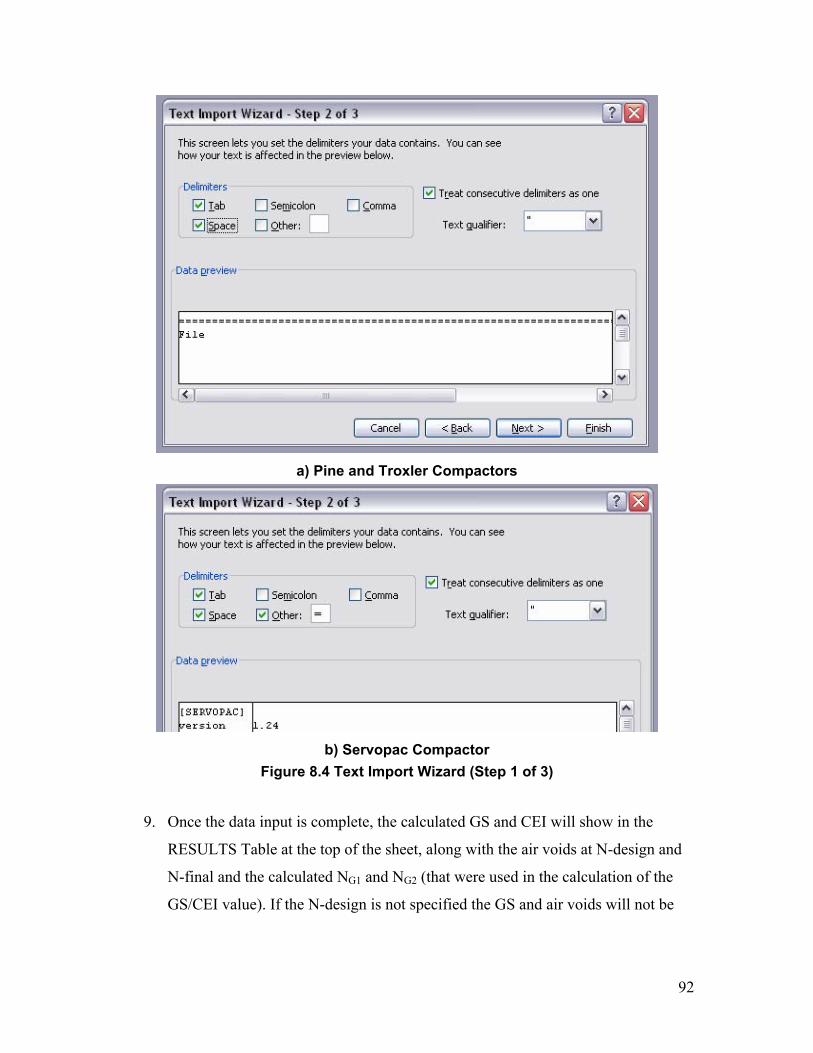
92
a) Pine and Troxler Compactors
b) Servopac Compactor
Figure 8.4 Text Import Wizard (Step 1 of 3)
9. Once the data input is complete, the calculated GS and CEI will show in the
RESULTS Table at the top of the sheet, along with the air voids at N-design and
N-final and the calculated NG1 and NG2 (that were used in the calculation of the
GS/CEI value). If the N-design is not specified the GS and air voids will not be
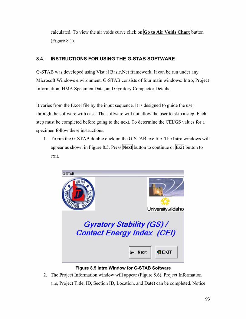
93
calculated. To view the air voids curve click on Go to Air Voids Chart button
(Figure 8.1).
8.4. INSTRUCTIONS FOR USING THE G-STAB SOFTWARE
G-STAB was developed using Visual Basic.Net framework. It can be run under any
Microsoft Windows environment. G-STAB consists of four main windows: Intro, Project
Information, HMA Specimen Data, and Gyratory Compactor Details.
It varies from the Excel file by the input sequence. It is designed to guide the user
through the software with ease. The software will not allow the user to skip a step. Each
step must be completed before going to the next. To determine the CEI/GS values for a
specimen follow these instructions:
1. To run the G-STAB double click on the G-STAB.exe file. The Intro windows will
appear as shown in Figure 8.5. Press Next button to continue or Exit button to
exit.
Figure 8.5 Intro Window for G-STAB Software
2. The Project Information window will appear (Figure 8.6). Project Information
(i.e, Project Title, ID, Section ID, Location, and Date) can be completed. Notice

94
the red square beside the HMA Data and Compactor Data buttons. This
indicates that the inputs for both section is not complete. In addition, the
Compactor Data button is not active. It will only be activated when the
specimen input data is completed.
Figure 8.6 Project Information Window for G-STAB Software
3. Press the HMA Data button to open the HMA Specimen Data window (Figure
8.7). Enter the required data in the designated boxes. When completed press the
Next button. Note that if the data is not complete, the software will prompt the
user to input the missing data. The HMA Specimen window will close and the
Project Information window will be reactivated. The red square beside the HMA
Data button will turn green indicating that specimen input data is completed and
the Compactor Data button is activated (Figure 8.8).

95
4. Press the Compactor Data button to open the Gyratory Compactor Details
window (Figure 8.9). This window consists of two parts: the first is for general
information about the compaction data; the second part is for the gyratory
compactor data.
Figure 8.7 HMA Specimen Data Window for G-STAB Software
Figure 8.8 Project Information Window when Specimen Data is completed

96
5. If the height of the load measuring device is included in the height measurement
while compaction, check the box beside “Height of PDA Included.” A box will
appear where one can input the height of the load cell (Figure 8.9). It’s essential
to subtract the height of the loading cell in order to calculate the actual air voids.
Figure 8.9 Gyratory Compactor Data Inputs Window for G-STAB Software
6. For Manual Inputs of Compaction Data (typically used if you are using an
external device to measure force, such as PDA), click on the Manual Inputs
button. The software will prompt the user to choose the type of loading: Shear
Stress or Vertical Force (Figure 8.10).
a. If “Shear Stress” is selected, two input boxes will appear. Input the height
and the shear stress versus the number of gyrations shown in the adjacent
box. Press Add Entry after each entry. The entered values will be shown
in the text box (Figure 8.10 a). The same process should be followed until

97
all values are entered. To edit any entry, press the Find Entry button, and
the software will prompt the user to input the number of gyrations for this
entry. The entry can be edited by re-entering the correct value. Then press
the Edit Entry button.
a) Shear Stress Inputs
b) Vertical Forces Inputs
Figure 8.10 Manual Inputs of Compaction Data

98
b. If “Vertical Force” is selected, two input boxes will appear. Input the
height and the vertical force versus the number of gyrations shown in the
adjacent box. Press Add Entry. The entered values will be shown in the
text box (Figure 8.10 b). The same process should be followed until all
values are entered. To edit any entry, press the Find Entry button, and
the software will prompt the user to input the number of gyration for this
entry. The entry can be edited by re-entering the correct value. Then press
the Edit Entry button.
7. For a manual inputs check, the total number of gyration should be entered in the
designated box as shown in Figure 8.10.
Figure 8.11 Importing Compaction Data form a Gyratory Output File

99
8. Importing Files from the Gyratory Compactor output file: G-STAB has been
developed for two types of compactors: Servopac and Pine Model AFG1. Click
on the appropriate button for the Gyratory compactor. The software will prompt
the user to choose the gyratory output file. When the data import is complete a
message will appear confirming the completion. In addition the imported data and
the total number of gyrations will be displayed as shown in Figure 8.11.
9. To determine GS, N-design should be entered in the designated box. To only
determine CEI, “0” must be entered in the N-design designated box.
10. When all data entries are completed press the Next button. Note that if the input
data is not complete, the software will prompt the user to input the missing data.
The Gyratory Compactor Details window will close and the Project Information
window will be reactivated. The red square beside the Compactor Data button
will turn green, indicating that specimen input data is completed and the button is
activated (Figure 8.11). In addition, the Run Analysis button will appear.
Figure 8.12 Project Information Window when All Data Entries are completed

100
11. Press the Run Analysis button. The software will calculate CEI/GS and a
message will appear when the calculations are complete. The calculated CEI/GS
values will be displayed as in Figure 8.12.
Figure 8.13 Project Information Window when the Analysis is Completed
12. For documentation, the calculation can be saved as a text file with a “*.cei” file
extension. This file will include all data inputs and air voids at each number of
gyrations. This file can be accessed for viewing or printing by any word document
program such as Notepad that is available in all Microsoft Windows
environments. To save, press the Save button (Figure 8.12), and the software will
prompt the user to choose a file name and location.
13. To start a new analysis, press the New button. If the previous analysis is not
saved, the software will only prompt the user to save the analysis once.
14. When finish, press the Exit button. If the previous analysis is not saved, the
software will only prompt the user to save the analysis once.

101
8.5. EXAMPLE
To demonstrate the procedure for CEI/GS calculations using both G-STAB and Excel file
and the variations between the two, one example is used.
8.5.1. Inputs
A trial HMA sample was mixed and compacted using the Pine compactor in the
laboratory as per Superpave specifications. The data required to determine CEI and GS
for this mix is listed in Table 8.1.
Table 8.1 Required Data for CEI/GS Calculations Maximum Theoretical Specific
Gravity (Gmm) 2.436
Final Bulk Specific Gravity (Gmb) 2.363 Mix Data
Final Weight of compacted
sample (dry weight) 4500 g
Vertical Stress 600 kPa
Gyration Angle 1.25°
Mold Diameter 150 mm
N-design 100
Compactor Data
Pine Gyratory Output File G48P1.dat
8.5.2. Using the Excel File
Using the data in Table 8.1, the above instructions were followed for determining the CEI
and GS values for this trial mix. The resulting GS and CEI values, as shown in Figure
8.14, are equal to15.61 kN.m and 18.56 kN.m, respectively. In addition, the air voids at
N-design were determined to be 3.7%, and 3.0% at N-final. The air void curve was
plotted as shown in Figure 8.15.

102
Figure 8.14 CEI and GS Calculation Results for the Trial Mix Using the Excel File
Figure 8.15 Air Voids Curve for the Trial Mix

103
8.5.3. Using the G-STAB Software
The instructions were also followed for determining the CEI and GS values using G-
STAB for the same trial mix and utilizing the data in Table 8.1. The resulting GS and
CEI values, as shown in Figure 8.16, are equal to15.59 kN.m and 18.54 kN.m,
respectively. In addition, all input data, calculation results, and change of height, air
voids, and Shear Stress versus gyration numbers can be saved as a text file as shown in
Figure 8.17.
Figure 8.16 CEI and GS Calculation Results for the Trial Mix Using G-STAB

104
Figure 8.17 Page 1 of G-STAB Output File
There is a minor difference between the results of G-STAB and that of the Excel file.
This is believed to be due to the different process for rounding numbers in each
framework.
105
9. SUMMARY AND CONCLUSIONS
9.1. SUMMARY
This research addressed the development of new testing methods that can be augmented
with the Superpave asphalt mix design system. Superpave was developed under the
Strategic Highway Research Program (SHRP). The research outcomes of SHRP included
state-of-the-art methods to design Hot-Mix Asphalt (HMA) based on performance.
However, and for practical implementation of SHRP products, the design criterion in the
current Superpave system is based only on volumetric analysis. There has been a need to
develop simple, practical and reliable methods and procedures to be incorporated in the
design criteria of Superpave. Research efforts since the release of Superpave in 1992
have continued to address this issue. A few test procedures and new performance
indicators have been developed.
The main goal of this study was to evaluate the potential of using the gyratory
compaction forces and deformation to measure the aggregate structure stability in hot-
mix asphalt (HMA) during the mix design process. This method is intended as a
screening tool to identify aggregate structures that have low resistance to applied forces
prior to conducting further performance testing. The measured compaction shear forces
and deformation of a wide spectrum of hot-mix asphalt (HMA) mixtures were used to
calculate a stability index referred to as the Gyratory Stability (GS). Further, this study
addressed the development and evaluation of the critical strain energy release rate Jc, as
an indicator of HMA resistance to fracture. Jc was determined from load-deformation
data of a simple three-point bending fracture test using notched semi-circular specimens.
The test specimens were prepared from standard Superpave Gyratory compacted HMA
samples.
In the first stage of this study, using forty-seven Hveem-designed mixes in Idaho, the GS
values of these mixes were compared to their Hveem Stability (HS) values. In addition,

106
the aggregate used in these mixes was evaluated using the Aggregate Imaging System
(AIMS), and the texture results were compared to the GS values. To evaluate the effect of
the HMA material properties on the variation of Jc, thirty-four mixes of the forty-seven
Hveem-designed mixes were used in the analysis. All mixes were designed and
constructed in accordance to the Hveem design method. Experimental results indicated
that CEI/GS and Jc are sensitive to mix design components including the asphalt binder
content and the aggregate structure.
In the second stage of this study, two Superpave-designed mixes were tested, to
investigate if the GS and Jc measurements could be used as screening tools at the mix
design stage to assess the mix performance, before implementing sophisticated and time-
consuming performance tests. Further, a Visual Basic software program and an Excel file
were developed to facilitate the calculation of GS and CEI.
9.2. CONCLUSIONS
Based upon the test results and data analysis presented in this research, the following
conclusions and observations are made:
9.2.1. Hveem-Designed Mixes
• The GS correlated well with the Hveem Stability of Hveem-designed mixes.
Results, however, showed wide variation in GS values for mixes that had the
same Hveem Stability. This may indicate that GS is more sensitive to changes in
mix design parameters than Hveem Stability. A three tier GS limits of 5, 12 and
15 are suggested to classify HMA mixtures based on their stability.
• Results of the APA rut testing did not correlate with the GS of these mixes. It is
believed that the main reason is that the current APA testing procedure allows
testing the mix at different temperatures based on its high temperature grade,
while the GS is determined at the standard compaction temperature of 149 °C. A
better correlation between GS and permanent deformation in APA was obtained
107
for mixes that have the same PG grade and tested at the same temperature in the
APA.
• Image analysis indicated that aggregate texture correlated with the GS. There was
no clear relationship between angularity and sphericity with GS for the range of
aggregates used in this study.
• The Jc measured by the semi-circular notched bending fracture (SCBNF) test can
represent HMA resistance to fracture. The SCBNF test is simple and quick to
perform, and can be implemented at the mix design stage of HMA design.
• Finite Element Analysis was used to model the SCBNF test configuration. FEA
results were used to calculate the mixture elastic modulus. The elastic modulus
was correlated to the Jc. Results indicate that Jc increases with the increase in
modulus values of HMA. It is postulated that Hveem mixes with higher stabilities
have higher stiffness, and therefore exhibit a higher resistance to fracture as
measured by the Jc parameter.
• Results have shown that KJC,which is equivalent to KIC, followed the same trend
as Jc for the tested mixes and the results fell into the range of reported KIC.
• The Jc parameter was found to be sensitive to changes in the mix aggregate
gradations and to the aggregate shape and surface texture properties as measured
by the Aggregate Imaging System (AIMS). Mix with finer aggregate gradations
showed higher resistance to fracture compared to the mix with coarser aggregate
gradations. Mixes with rougher aggregate texture and more angular particles
showed higher Jc values. Mixes that had high percentages of flattened and
elongated aggregates showed lower Jc values.
• The Jc parameter was found to be sensitive to variation in the asphalt binder
content. Results showed that as the binder content increased the value of Jc
increased. However, no clear trend was found that relates Jc to different binder
grades.
108
• Overall, this study concludes that Jc determined in a SCNBF test can be used to
assess a HMA mixture’s propensity to fracture during the design stage.
9.2.2. Superpave-Designed Mixes
• Based on the two mixes evaluated by means of GS and Jc, it was found that Mix 2
performs better than Mix 1 under the same loading conditions.
• GS was found to be sensitive to asphalt content but not to asphalt binder grade.
This is attributed to the compacting temperatures at which GS is determined.
• GS determined at optimum asphalt content was the highest for both mixes.
• GS correlated well with the APA test results with a reported R2 equal to 0.58. It
was observed that the higher the GS values the lower the permanent deformation
the mix will endure, as determined by APA.
• The rutting parameter (E*/sin φ) at both 130 °F and 100 °F correlated with the
GS, with an R2 equal to 0.76 and 0.65, respectively. In addition, GS correlated
well with the Flow Number results with a reported R2 equal to 0.49.
• The Jc was found to be sensitive to the variation in the asphalt binder content. It
was found that there is no clear relationship between the optimum asphalt content
and Jc.
• There was no clear trend between Jc and the fatigue indicator (E*.sin φ) at both
70° F and 40 °F when both mixes are compared. But within each mix, both
parameters followed the same trends.

109
REFERENCES
AASHTO Designation TP 62-03. (2004). “Standard Method of Test For Determining Dynamic Modulus of Hot-Mix Asphalt Concrete Mixtures.” American Association of State Highway and Transportation Officials.
Abdulshafi, A. and K. Majidzadeh. (1985). “J-Integral and Cyclic Plasticity Approach to Fatigue and Fracture of Asphalt Mixtures.” Transportation Research Record 1034, Transportation Research Board, National Research Council, Washington, D.C.
Abu Abdo, A. (2005). “Development of Performance Parameters for the Design of Hot-Mix Asphalt.” Master Thesis, University of Idaho, Moscow, Idaho.
ALGOR, FEMPRO Version 13.24-WIN 28-OCT-2002. ALGOR, Inc., Pittsburgh, PA.
Anderson, R., P. Tuner, R. Peterson, and R. Mallick. (2002). “Relationship of Superpave Gyratory Compaction Properties to HMA Rutting Behavior.” NCHRP Report 478, TRB, Washington, D.C.
Australian Standards – AS/NZS 2891.2.2. (1995). “Methods of Sampling and Testing Asphalt, Method 2.2 Sample Preparation - Compaction of Asphalt Test Specimens Using a Gyratory Compactor.”
Bahia, H., T. Friemel, P. Peterson, J. Russell, and B. Poehnelt. (2003). “Optimization of Contractibility and Resistance to Traffic: A New Design Approach for HMA Using the Superpave Compactor.” Journal of Association of Asphalt Paving Technologists, Vol. 72.
Bahia, H., E. Masad, A. Stackston, S. Dessouky, and F. Bayomy. (2003). “Simplistic Mixture Design Using the SGC and the DSR.” Proceedings of the Association of Asphalt Paving Technologists, Vol. 72, pp 196-225.
Bayomy, F., E. Masad, and S. Dessouky. (2002). “Development and Performance Prediction of Idaho Superpave Mixes.” Interim Report ITD-NIATT Project KLK464, National Institute for Advanced Transportation Technology, University of Idaho, Moscow, Idaho.
Bhasin, A., J.W. Button, and A. Chowdhury. (2004). “Evaluation of Simple Performance tests on Hot-Mix Mixtures from The South Central United States.” Transportation Research Record 1891, TRB, Washington, D.C.
Bhurke, A., E. Shin and L. Drzal. (1997)."Fracture Morphology and Fracture Toughness Measurement of Polymer Modified Asphalt Concrete." 76th annual meeting of the Transportation Research Board, Paper No. 970942.
Binaquist, R.F., D.W. Christensen, and W. Stump. (2003). “Simple Performance Tester for Superpave Mix Design: First-Article Development and Evaluation.” NCHRP Report 513, TRB, Washington, D.C.

110
Butcher, M. (1998.) “Determining Gyratory Compaction Characteristic Using Servopac Gyratory Compactor.” Transportation Research Record 1630, TRB, Washington, D.C.
Choubane, B., G. Page, and J. Musselman. (2000). “Suitability of Asphalt Pavement Analyzer for Predicting Pavement Rutting.” Transportation Research Record 1723, TRB, Washington, D.C.
Cominsky, J., G. Huber, T. Kennedy, and R. Anderson. (1994). “The Superpave Mix Design Manual for New Construction and Overlays.” SHRP Report A-407, Strategic Highway Research Program, Washington, D.C.
Dessouky, S., E. Masad, and F. Bayomy. (2004). “Prediction of Hot Mix Asphalt Stability Using the Superpave Gyratory Compactor,” Journal of Materials in Civil Engineering, Vol. 16, No. 6.
DeSombre, R., B. Chadbourn, D.E. Newcomb, and V. Voller. (1998.) “Parameters to Define the Laboratory Compaction Temperature Range of Hot-Mix Asphalt.” Journal of Association of Asphalt Paving Technologists, Vol. 67.
Dongre, R., M.G. Sharma, and D.A. Anderson. (1989). “Development of Fracture Criterion for Asphalt Mixes at Low Temperatures.” Transportation Research Record 1228, TRB, National Research Council, Washington, D.C.
Faheem, A.F., H.U. Bahia, and H. Ajideh. (2005). “Estimating Results of a Proposed Simple Performance Test for Hot-Mix Asphalt from Superpave Gyratory Compactor Results.” Transportation Research Record 1929, TRB, Washington, D.C.
Fletcher, T., C. Chandan, E. Masad, K. Sivakumar. (2003). “Aggregate Imaging System (AIMS) for Characterizing the Shape of Fine and Coarse Aggregates.” Transportation Research Record 1832, Transportation Research Board, National Research Council, Washington D.C.
Guler, M., H. Bahia, P. Bosscher, and M. Plesha. (2000). “Device for Measuring Shear Resistance for Hot Mix Asphalt in Gyratory Compactor.” Transportation Research Record 1723, TRB, Washington, D.C.
Huang, B., W. Kingery, Z. Zhang, and G. Zuo. (2004). “Laboratory Study of Fatigue Characteristics of HMA Surface Mixtures Containing Rap.” Presented at 83rd Annual Meeting of the Transportation Research Board, Washington, D.C.
Huang, Y.H. (2004). Pavement Analysis and Design. Pearson Prentice Hall, Second Edition, New Jersey.
Idaho Department of Transportation. “Standard Specifications for Highway Construction.” Boise, Idaho.
Kumar A., and W. Goetz. (1974). “The Gyratory Testing Machine as a Design Tool and Instrument for Bituminous Mixture Evaluation.” Asphalt Paving Technology, Vol. 43.
111
Landes, J., and D. McCabe. (1984). “Effect of Section Size on Transition Temperature Behavior of Structural Steel.” ASTM STP 833.ASTM International, West Conshohocken, PA.
Li, X., and M. Marasteanu. (2004). “Evaluation of Low Temperature Fracture Resistance of Asphalt Mixture Using the Semi Circular Bend Test.” Journal of the Association of Asphalt Paving Technologists, Vol. 73.
Lim, I.L., I.W. Johnston, S.K. Choi, and J.N. Boland. (1994). “Fracture Testing of a Soft Rock with Semi-Circular Specimens Under Three-point Bending. Part 1-Mode I.” International Journal of Rock Mechanics and Mining Science, Vol. 31, No. 3.
Little, N. and K. Mahboub. (1985). “Engineering Properties of First Generation Plasticized Sulfur Binders and Low Temperature Fracture Evaluation of Plasticized Sulfur Paving Mixtures.” Transportation Research Record 1034, TRB, National Research Council, Washington, D.C.
Mallick, R. (1999). “Use of Superpave Gyratory Compactor to Characterize Hot Mix Asphalt.” Transportation Research Record 1681, TRB, Washington, D.C.
Martin, A. and D. Park. (2003). “Use of the Asphalt Pavement Analyzer and Repeated Simple Shear Test at Constant Height to Augment Superpave Volumetric Mix Design.” Journal of Transportation Engineering, Vol. 129, No. 5.
Masad, E. (2003). “The Development of A Computer Controlled Image Analysis System for Measuring Aggregate Shape Properties.” NCHRP-IDEA Project 77 Final Report, Transportation Research Board, Washington, D.C.
Masad, E., D. Little, and R. Sukhwani. (2004). “Sensitivity of HMA Performance to Aggregate Shape Measured Using Conventional and Image Analysis Methods.” International Journal of Road Materials and Pavement Design. Vol. 5, No. 4.
McCabe, D., J. Merkle, and K. Walin. (2005). “An Introduction to the Development and Use of the Master Curve Method.” ASTM MNL52, ASTM International, West Conshohocken, PA.
McRea, J.L. (1962). “Gyratory Compaction Method for Determining Density Requirements for Subgrade and Base of Flexible Pavements.” Miscellaneous Paper No. 4-494, U.S. Army Engineering Waterways Experiment Station, Corps of Engineering, Vicksburg, MS.
McRea, J.L. (1965). “Gyratory Testing Machine Technical Manual.” Engineering Developments Company Inc., Vicksburg, MS.
Mohammad, L.N., Z. Wu, and M. A. Mull. (2004). “Characterization of Fracture and Fatigue Resistance on Recycled Polymer-Modified Asphalt Pavements.” 5th RILEM International Conference on Cracking in Pavements. Limoges, France.
Molennar, A., A. Scarpas, X. Liu, and G. Erkens. (2002). “Semi Circular Test; Simple but Useful?” Journal of the Association of Asphalt Paving Technologists, Vol. 71.

112
Mull, M., K. Stuart, and A. Yehia. (2002). “Fracture Resistance Characterization of Chemically Modified Crumb Rubber Asphalt Pavement.” Journal of Materials Science, Vol. 37.
Mull, M. A., A. Othman, and L. Mohammad. (2004). “Fatigue Crack Propagation Analysis of Chemically Modified Crumb Rubber Asphalt Mixtures.” Journal of Elastomers and Plastics. Vol 37.
Ott, R.L. and M. Longnecker. (2001). An Introduction to Statistical Methods and Data Analysis. Fifth Edition. Duxbury, Pacific Grove, CA.
“Pressure Distribution Analyzer (PDA).” Test Quip Inc., http://www.testquip.com, Minneapolis, Mn.
Rand, D. (1997). “Comparative Analysis of Superpave Gyratory Compactors and TxDOT Gyratory Compactors.” Master Thesis, University of Texas, Austin, TX.
Rice, J.R. (1968). “A Path Independent Integral and the Approximate Analysis of Strain Concentration by Notches and Cracks.” Journal of Applied Mechanics, Vol. 35.
Ruth, B., X. Shen, and L. Wang. (1991). “Gyratory Evaluation of Aggregate Blends to Determine their Effects on Shear Resistance and Sensitivity to Asphalt Content.” American Society for Testing and Materials, 1147.
Segerlind, L.J. (1984). Applied Finite Element Analysis. John Wiley and Sons Inc., Second Edition, New York, NY.
Sigurjonsson, S., B. Ruth. (1990). “Use of Gyratory Testing Machine to Evaluate Shear Resistance of Asphalt Paving Mixture.” Transportation Research Record 1259, TRB, Washington, D.C.
Stackston, A., J. Bushek, and H. Bahia. (2002). “Effect of Fine Aggregates Angularity (FAA) on Compaction and Shearing Resistance of Asphalt Mixtures.” Presented at TRB 81st Annual Meeting, Washington, D.C.
Tandon, V., B.S. Kambham, R., Bonaquist and M. Solaimanian. (2004). “Results of Integrating Simple Performance Tests and Environmental Conditioning System.” Transportation Research Record 1891, TRB, Washington, D.C.
Van de Ven, M., A. de Fortier Smit, and R. Krans. (1997). “Possibilities of a Semi-Circular Bending Test.” Proceedings of the Eighth International Conference on Asphalt Pavements, Vol. II, Seattle, WA.
Witczak, M., K. Kaloush, T. Pellinen, M. Al-Basyouny, and H. Von Quintus. (2002). “Simple Performance Test for Superpave Mix Design.” NCHRP Report 465, TRB, Washington, D.C.
Zborowski, A., A. Sotil, K.E. Kaloush, and G.B. Way. (2002). “Material Characteristics of Asphalt Material.” TRB 83rd Annual meeting CD-ROM, Washington, D.C.

113
APPENDICES
Appendix A: Mix Design Details and Job Mix Formula (JMF) for All Mixes. This is provided in PDF
on the attached CD
Appendix B: Gyratory Stability and Gyratory Compaction Data Files. Provided on the attached CD.
Appendix C: CEI and GS Software. Provided on the attached CD.