performance evaluation of commodity investments

Performance evaluation of commodity investments

Dimitrios I. Vortelinos∗and Hanxiong Zhang †

March 30, 2016

Abstract

This paper extends a still ongoing debate on whether the choice of the performance measure influ-

ences the evaluation of investments by investigating the daily returns of 10 spots-based commodities

and 16 futures-based commodities. We find that the choice of performance measures and samples do

affect the rankings of commodity investments. There are commodities that show substantial changes

in ranking if the performance measure is changed from the Sharpe ratio to an alternative measure.

Our findings are robust in 6 unequal length subsamples, which reflect different market conditions.

Given that a large number of commodity traders use margin trading and the volatility of commodity

is very high, we argue that the use of multi performance measures, high frequency data, and multi

market condition subsamples could has a positive influence on the commodity investment.

Keywords: Investment evaluation; Sharpe ratio; Commodities; Spot; Futures.

JEL Classification: C10; D81; G11; G29.

∗Corresponding author. Lincoln Business School, University of Lincoln, UK. Contact at [email protected],0044-1522-835634 (tel.).†Lincoln Business School, University of Lincoln, UK. Contact at [email protected], 0044-1522-835639 (tel.).

1

1 Introduction

In this paper we extend a still ongoing debate on whether the choice of the performance measure influences

the evaluation of investments by investigating the daily returns of 10 spots-based commodities and

16 futures-based commodities. This research question is interesting for a variety of audiences. For

investment practitioners, they can select any measure they think can marketing their financial products

best to investors. They can even turn to the simplest and most popular performance measure on the

purpose of selecting the best investments within a set of given alternatives (Auer, 2015). For regulators,

they can assess how practitioners should best present financial performances without misleading the

information users. Researchers could gain insight into effectiveness of the existing performance measures

which, in turn, enable them to develop more sophisticated performance measures accordingly.

The Sharpe ratio, defined as the mean excess return over the standard deviation of the returns gen-

erated by the investment (Sharpe, 1966), is the simplest and most popular performance measure for

the financial investment industry. Sharpe ratio is competent only for normally distributed investment

returns. Unfortunately, it is quite common to observe that investment returns are non-normally dis-

tributed (Eling and Schuhmacher, 2007). Even worse, Sharpe ratio is prone to manipulation and suffers

from a number of technical biases. For example, some option-based strategies that maximize the Sharpe

ratio but do not necessarily add value to the investor (Goetzmann et al., 2007). Under certain condi-

tions, a very high return in a prospective period is penalized by a lower realization of the Sharpe ratio,

because, intuitively, an investor would expect the Sharpe ratio to increase in such a situation (Schuster

and Auer, 2012). Alternatively, one can rise the Sharpe ratio by generating an extremely negative excess

return (Auer, 2013). Consequently, a large number of alternative performance measures emerged for the

purpose of overcoming the limitations of Sharpe ratio.

Pedersen and Rudholm-Alfvin (2003), Eling and Schuhmacher (2007) and Eling (2008) examine

the Sharpe ratio with a number of alternative performance measures (reward-to-risk ratios based on

drawdowns, partial moments, and the Value at Risk (VaR)) through a variety of asset class datasets,

and surprisingly find almost identical rank orderings across investments. These findings quickly stimulate

further theoretical and empirical investigations.

From a theoretical perspective, Schuhmacher and Eling (2011) and Schuhmacher and Eling (2012)

argue that if investment returns meet the location and scale (LS) condition of Sinn (1983) and Meyer

(1987), the Sharpe ratio, adequately defined drawdown-based performance measure and certain perfor-

mance measures based on partial moment, the VaR and other risk quantities yield identical rankings.

Given that the location and scale (LS) condition is not satisfied by cross-sectionally different levels of

skewness and kurtosis in financial investment returns data (Agarwal and Naik, 2004), it cannot suffi-

ciently interpret the empirically observable ranking similarities (Auer and Schuhmacher, 2013).

From an empirical perspective, the findings are mixed. For example, Zakamouline (2011) reinves-

2

tigates the findings of Eling and Schuhmacher (2007) using one of their German hedge fund datasets.

Through calculating the maximum upgrade, maximum downgrade, mean absolute change, and standard

deviation of the change in the rankings, Zakamouline (2011) argues that a high rank correlation coef-

ficient does not necessarily yield almost identical fund ranking orders, given that there are funds that

show substantial changes in ranking if the performance measure is changed from the Sharpe ratio to

an alternative measure. Ornelas et al. (2012) reinvestigate the findings of Eling (2008) using the US

mutual fund dataset, and suggest that different performance measures do not yield similar rankings if

their mean excess returns (numerators) are different. On the contrary, Eling et al. (2011) find that

the choice of performance measure does not matter when they are tailored to a moderate investment

style. However, when they are applied to investigate aggressive investment styles, rank correlations with

the Sharpe ratio decrease significantly. Auer and Schuhmacher (2013) find that the adequately defined

drawdown-based performance measures yields hedge fund rankings not too different from those shown

with the Sharpe ratio when investors are primarily interested in picking the best investments and when

a long return sample is applied to calculate performance measure estimates. While, the rankings are

not strictly identical when small return sample is employed to evaluate hedge funds. Beyond the mutual

fund and hedge fund datasets, Auer (2015) finds that the Sharpe ratio and 12 alternative performance

measures based on drawdowns, partial moments, and the VaR yield almost identical rank orderings

across 30 futures-based commodity investments. Auer (2015) also argues that his empirical findings are

robust in several dimensions, for instance, the dataset, the time period, the return calculation method

and the performance measure parametrization.

This paper contributes to the literature from several perspectives. First, we are the first to study

whether the choice of the performance measure influences the evaluation of spots-based commodity in-

vestments. Even though Auer (2015) provides deep insight into 30 futures-based commodity investments,

commodity investments remain under-studied relative to stocks, bonds, even mutual funds and hedge

funds. In particular, it remains unclear whether Auerâs (2015) findings are justified by the spots-based

commodity investments. Investment returns in the spots and futures market differ from one another

as a result of the disparity in the timing of delivery of the underlying goods. Buying or selling of the

physical commodities for immediate delivery occur at a price that both buyer and seller will refer to is

the spots-based commodity price. In contrast, the price for the purchases or sales of future obligations to

make or take delivery rather than the physical commodities is futures-based commodity price. The costs

associated with carrying the physical commodities until the agreed delivery date is the cost to carry.

When the market is in equilibrium, future price is the sum of spot price and total carrying costs (in-

cluding dividend, convenience yield, storage cost, and cost of money). Futures-based commodity prices

are regarded as more volatile than spots-based commodity prices due to lower trading costs and ease

of shorting. Although conventional wisdom argues that futures markets perform the function of price

3

discovery, the empirical findings are mixed (Silvapulle and Moosa, 1999; Pindyck, 2001; Garner, 2012).

Second, contrast to existing literature (Auer and Schuhmacher, 2013; Auer, 2015), which investigate

the ranking similarities over time by simply splitting full investment returns sample into a number of equal

length subsamples. We divide the full sample into 6 unequal length subsamples according to the market

conditions as defined in literature, namely, 1 growth subsample and 5 crisis subsamples. The rationale

for distinguishing market conditions is driven by the fact that there is an increase in the correlation

between investment assets during volatile periods (Loretan and English, 2000; Ang and Bekaert, 2002).

Amira et al. (2011) argues that the increase in the correlation is driven by the historical return and

the market direction rather than the volatility. If the returns sample is typically recession, then not

only may the estimated volatilities be too high, but, perhaps the estimated ranking correlations will be

higher than average. However, it remains unclear whether the market conditions influences the choice of

performance measure.

Third, contrast to the majority of literature (Eling and Schuhmacher, 2007; Eling, 2008; Eling et

al., 2011; Zakamouline, 2011; Auer and Schuhmacher, 2013; Auer, 2015)1, we use daily data instead of

monthly data. This is because daily data react much quicker to the arrival of new information and thereby

yield greater precision in the estimates of the investment risk (Burghardt and Walls, 2011). For monthly

data, even fairly large changes in market conditions would require longer time to detect. Considered that

commodities’ high volatility and a large number of commodity investors use margin trading, investors

might be kicked out from the market even in the case of monthly return is zero. Therefore, daily data is

superior to the monthly data in quantifying the investment risk.

Overall, our empirical findings suggest that the choice of performance measure matters for both of

spots- and futures-based commodity investment, which is roughly in line with Ornelas et al. (2012) and

Zakamouline (2011) but contrast to Auer and Schuhmacher (2013) and others, especially Auer (2015).

The reminder of the paper is organized as follows: Section 2 describes main features of our data.

Section 3 presents empirical methodology. Section 4 shows the empirical results and robustness checks.

Section 5 concludes the paper.

2 Data

In this paper, we use a dataset consisting of daily data for 10 spots-based commodities and 16 futures-

based commoditiesâ prices over the sample from 1st September 1998 through 22nd August 2014. All

commodity prices are denominated in US Dollar. Our spots-based commodities dataset covers 10 metal

commodities (zinc, tin, silver, platinum, palladium, nickel, lead, copper, gold, aluminum). Our futures-

based commodities dataset includes 5 energy commodities (natural gas, heating oil, gasoline, crude oil,1Ornelas et al. (2012) use both monthly and daily data to study the choice of performance measure for ranking of US

mutual funds. The rest of relevant literature use monthly data only.

4

and Brent crude oil) and 11 soft commodities (wool, wheat, sugar, soybeans, rubber, rice, oat, cotton,

corn, coffee, cocoa). We obtain the real-time commodities prices from the Trading Economics. The

selection of spots- and futures-based commodities are determined by the availability of data at the

Trading Economics. We calculate the daily investment return as equation (1).

rt=lnPt − lnPt−1 (1)

where, Pt is the spot price of commodity on day t, ln denotes for natural log. We calculate the excess

returns of these commodity investments using the daily 10-year US government bond yield as a proxy

for the daily risk-free rate instead of the 1-month Treasury bill rate as in Auer and Schuhmacher (2013)

and Auer (2015). This is because the typical commodity traders in particular oil producers, usually have

a much longer investment horizon and higher opportunity cost than the typical mutual fund investors.

Our sample size is roughly comparable to Auer (2015), which uses monthly futures-based commodity

data over the sample from January 2002 to September 2013.

2.1 Data description

In this subsection, there is a short description of each of commodities.

2.1.1 Energy commodities

Energy commodities have been recently researched by Doran and Ronn (2008). The time series properties

of crude oil were examined in Sevi (2015). In the present study, Brent crude oil, crude oil, gas, gasoline

and heating oil are the energy commidities evaluated.

Natural gas price is measured in USD/MMBtu. MMBtu equals to 1 million BTU (British thermal

unit) and is standardized to 28.263682 m3 of natural gas at defined temperature and pressure. Natural

gas accounts for almost a quarter of United States energy consumption, and the NYMEX Division natural

gas futures contract is widely used as a national benchmark price. The futures contract trades in units

of 10,000 million British thermal units (mmBtu). The price is based on delivery at the Henry Hub in

Louisiana, the nexus of 16 intra- and interstate natural gas pipeline systems that draw supplies from

the regionâs prolific gas deposits. The pipelines serve markets throughout the U.S. East Coast, the Gulf

Coast, the Midwest, and up to the Canadian border.

Heating oil price is measured in USD/GAL. A gallon is 231 cubic inches or approximately 3.785 liters

for liquids. It is also known as No. 2 fuel oil, accounts for about 25% of the yield of a barrel of crude,

the second largest âcutâ after gasoline. The heating oil futures contract trades in units of 42,000 gallons

(1,000 barrels) and is based on delivery in New York harbor, the principal cash market trading center.

Options on futures, calendar spread options contracts, crack spread options contracts, and average price

5

options contracts give market participants even greater flexibility in managing price risk. The heating

oil futures contract is also used to hedge diesel fuel and jet fuel, both of which trade in the cash market

at an often stable premium to NYMEX Division New York harbor heating oil futures.

Gasoline (US dollars per gallon) is the largest single volume refined product sold in the United

States and accounts for almost half of national oil consumption. The NYMEX Division New York

harbor unleaded gasoline futures contract and reformulated gasoline blend stock for oxygen blending

(RBOB) futures contract trade in units of 42,000 gallons (1,000 barrels). They are based on delivery

at petroleum products terminals in the harbor, the major East Coast trading center for imports and

domestic shipments from refineries in the New York harbor area or from the Gulf Coast refining centers.

Crude oil price is measured in US Dollar per BBL. BBL is defined as 42 US gallons, which is about

159 litres or 35 imperial gallons, and it can also be defined in those units, depending on the context.

Crude oil is the worldâs most actively traded commodity, and the NYMEX Division light, sweet crude

oil futures contract is the worldâs most liquid forum for crude oil trading, as well as the worldâs largest-

volume futures contract trading on a physical commodity. Because of its excellent liquidity and price

transparency, the contract is used as a principal international pricing benchmark. The contract trades

in units of 1,000 barrels, and the delivery point is Cushing, Oklahoma, which is also accessible to the

international spot markets via pipelines.

Brent crude oil (USD/BBL) is sourced from the North Sea. The name âBrentâ comes from the naming

policy of Shell Oil, which originally named all of its fields after birds (in this case the Brent Goose). Oil

production from Europe, Africa and the Middle East flowing West tends to be priced relative to this oil,

i.e. it forms a benchmark. However, large parts of Europe now receive their oil from the former Soviet

Union especially through Russia.

2.1.2 Metals

Precious metals have been recently researched in Caporin, Ranaldo and Velo (2015). Recently, the time

series properties of gold were investigated in Kristjanpoller and Minutolo (2015). In the present paper,

aluminium, copper, gold, lead, nickel, palladium, platinum, silver, tin and zinc are the metals researched.

Aluminium price is measured in USD/LB. Roman libra (LB), also knwon as libra pondo or pound,

is 0.45359237 kilograms. Aluminium is a lightweight, corrosion resistant metal used mainly in aerospace

applications, as a construction material, in packaging, automobiles and railroad cars. Resources of

bauxites, the raw material for aluminum are only located in seven areas: Western and Central Africa

(mostly, Guinea), South America (Brazil, Venezuela, Suriname), the Caribbean (Jamaica), Oceania and

Southern Asia (Australia, India), China, the Mediterranean (Greece, Turkey) and the Urals (Russia).

Aluminum futures and options contracts provide price transparency to the U.S. aluminum market, valued

at about $35 billion per year in products and exports.

6

Copper (USD/MT) is another metal important fot international markets. Chile accounts for over

one third of world’s copper production followed by China, Peru, United States, Australia, Indonesia,

Zambia, Canada and Poland. Major exporters of copper ores and concentrates are Chile, Peru, In-

donesia, Australia , Canada, Brazil, Kazakhstan, United States, Argentina and Mongolia. The biggest

importers of copper are China, Japan, India, South Korea and Germany. Copper market participants

use the COMEX Division of high-grade copper futures and options to mitigate price risk. Copper is the

world’s third most widely used metal, after iron and aluminum, and is primarily used in highly cyclical

industries such as construction and industrial machinery manufacturing. Profitable extraction of the

metal depends on cost-efficient high-volume mining techniques, and supply is sensitive to the political

situation particularly in those countries where copper mining is a government-controlled enterprise.

Gold price is measured in USD/t oz. The biggest producers of gold are China, Australia, United

States, South Africa, Russia, Peru and Indonesia. The biggest consumers of gold jewelry are India,

China, United States, Turkey, Saudi Arabia, Russia and UAE. Gold Futures are available for Trading

in the Commodity Exchange (COMEX) which merged with the New York Mercantile exchange in 1994

and became the division responsible for metals trading. Half of the gold consumption in the world is in

jewelry, 40% in investments, and 10% in industry. However, Gold is not only a precious metal but also a

commodity vital for many industries. Gold is an excellent conductor of electricity, is extremely resistant

to corrosion, and is one of the most chemically stable of the elements, making it critically important in

electronics and other high-tech applications.

Lead (USD/MT) is a soft, malleable, ductile, bluish-white, dense metallic element, extracted from

galena and found in ore with zinc, silver and copper. 80 percent of modern lead usage is in the production

of batteries. Lead is also often used to line tanks that store corrosive liquids and as a shield against

X and gamma-ray radiation. The biggest producers of lead are Australia, China and USA, followed by

Peru, Canada, Mexico, Sweden, Morocco, South Africa and North Korea. Lead Futures are available for

trading in The London Metal Exchange (LME). The standard contact has a size of 25 tonnes.

Nickel (USD/MT) is mainly used in the production of stainless steel and other alloys and can be

found in food preparation equipment, mobile phones, medical equipment, transport, buildings, power

generation. The biggest producers of nickel are Russia, Canada, New Caledonia, Australia, Indonesia,

Cuba, China, South Africa, Dominican Republic, Botswana, Columbia, Greece and Brazil. Nickel futures

are available for trading in The London Metal Exchange (LME). The standard contact has a weight of

6 tonnes.

Palladium (USD/t oz.) is a soft silver-white metal used mostly in the production of catalytic convert-

ers, electronics, dentistry, medicine, hydrogen purification, chemical applications, groundwater treatment

and jewelry. The biggest producers of palladium are by fat Russia and South Africa followed by United

States, Canada and Zimbabwe. Palladium Futures are available for trading in London Platinum and

7

Palladium Market and on the New York Mercantile Exchange. The standard contact weights 100 troy

ounces.

Platinum (USD/t oz.) is among the world’s scarcest metals. Supplies of platinum are concentrated

in South Africa, which accounts for approximately 80% of supply; Russia, 11%; and North America,

6%. Because of the metal’s importance as an industrial material, its relatively low production, and

concentration among a few suppliers, prices can be volatile. For this reason, it is often considered

attractive to investors.

Silver price is measured in US cents/t oz. Troy ounce (t oz) is a mass unit of troy weight system,

is commonly used in measuring silver and other precious metals. 1 troy ounce is equal to 31.1034768

grams, or 1/12 per troy pound. In fact, the London silver fixing prices are fixed based on the unit of troy

ounce; therefore, the silver prices of this website use the unit of troy ounce. Silver is a precious metal

that plays a role in investment portfolios. The largest industrial users of silver are the photographic,

jewelry, and electronic industries. The biggest producer of silver are: Mexico, Peru and China followed

by Australia, Chile, Bolivia, United States, Poland and Russia.

Tin (USD/MT) is a silvery, malleable metal mainly used in the production of solder and to coat

other metals to prevent corrosion. The biggest producers of tin are China, Malaysia, Indonesia, Peru,

Thailand, Bolivia and Belgium. Tin Futures are available for trading in The London Metal Exchange

(LME). The standard contact weights 5 tonnes.

Zinc price is measured in USD/MT; whereas, MT is an alternative term for tonne, a measurement

of mass equal to one thousand kilograms. Zinc is a lightweight and corrosion-resistant metal. It is often

used in die-casting alloys, castings, brass products, sheeting products, chemicals, medicine, paints and

batteries. The biggest producers of zinc are. China, Peru, Australia, United States, Canada, India and

Kazakhstan. Zinc Futures are available for trading in The London Metal Exchange (LME). The standard

contact weights 25 tonnes.

2.1.3 Soft commodities

Not many papers have recently researched soft commodities. Here, cocoa, coffee, corn, cotton, oat, rice,

rubber, soybeans, sugar, wheat and wool are researched.

Cocoa price is measured in US dollar (USD) per metric tonne (MT). The biggest producers of cocoa in

the world are Cote d’Ivoire (34% of total in 2009/10 fiscal year), Ghana (17%), Indonesia (15%), Nigeria,

Cameroon, Ecuador and Brazil. Cocoa has a wide variety of uses, from chocolate to cocoa butter to

coloring agents for food products. Although cocoa is one of the world’s smallest soft commodity markets,

it has global implications on cocoa importers and exporters, food and candy producers, and the retail

industry. The size of each contract is 10 metric tons and its commodity code is CJ. It is financially settled,

and the final settlement price will be set at the value of New York Board of Trade cocoa futures contract

8

on the termination day of the contract month, or as specified by the NYMEX Board of Directors.

Coffee price is measured in US cents per lb. Brazil is the biggest producer and exporter of coffee in

the world; 33% of total production from September 2010 to August 2011. Colombia, India, Indonesia,

Guatemala, Ethiopia, Mexico are also major producers. Coffee futures contracts that trade on the Inter

Continental Exchange (ICE) are the world benchmark for Arabica coffee. The word “coffee” is believed

to be come from Kaffe, Ehtiopia, where coffee originated in the 9th century. Derived from the coffee

bean, it was not well-received, and at one time was even banned in Turkey and Egypt. The demand for

coffee gradually increased until it has become one of the most popular beverages in the world.

Corn (USD/BU) is important for international trade and financial markets. Corn Futures are available

for Trading in The Chicago Board of Trade (CBOT R© ) which was established in 1848 and is a leading

futures and futures-options exchange. More than 3,600 CBOT member/stockholders trade 50 different

futures and options products at the CBOT by open auction and electronically.

Cotton price is measured in US cents per lb. The biggest producers of cotton in the world are China

(26% of total production in 2010/11 fiscal year) and India (22%), followed by United States, Pakistan,

Brazil, Australia and Uzbekistan. The United States is the biggest exporter of cotton (40% of total

exports). India, Australia, Brazil and Uzbekistan also have a big share in the cotton trade. Cotton, a

soft fiber that grows around the cotton plant, is the world’s most widely-used natural fiber for clothing.To

maximize the needs of the cotton market, the New York Mercantile Exchange has made available a cocoa

futures contract for trading on the CME Globex R© trading platform and for clearing through NYMEX

ClearPort R© clearing. The size of each contract is 50,000 pounds and its commodity code is TT. It is

financially settled, and the final settlement price shall be set at the value of the New York Board of Trade

cotton futures contract on the termination day of the contract month, or as specified by the Board of

Directors.

Oat price is measured in US cents (USX) per Bushel; whereas for oat, bushel is 32 lb or 14.5150 kilo-

grams (Kgs). Oat is a species of cereal grain used mainly as a livestock feed and for human consumption.

The biggest producers of oat are: European Union, Russia, Canada, Australia and United States. Oat

Futures are available for trading in the Chicago Mercantile Exchange. The standard contract has 5,000

bushels, the equivalent 86 metric tons.

Rice is measured in USD per CWT; whereas, CWT is entitled hundredweight that equals to 100

pounds. China is the biggest producer of rice in the world (30% of total production in 2010/11 fiscal

year), followed by India (21%), Indonesia (8%), Bangladesh (7%), Vietnam and Thailand. Biggest

exporters of rice include Thailand (30% of total exports), Vietnam (20%), India (11%) and the United

States (10%). The biggest consumer of rice is China, followed by India, Indonesia, Bangladesh and

Vietnam. Rice Futures are available for Trading in The Chicago Board of Trade (CBOT R© ) which

was established in 1848 and is a leading futures and futures-options exchange. More than 3,600 CBOT

9

member/stockholders trade 50 different futures and options products at the CBOT by open auction and

electronically.

Natural rubber price is measured in Malaysian ringgit (MYR) per kilogram (Kg). Rubber is a high

resilience, extremely waterproof and stretchable material. Is used extensively in many applications and

products, either alone or in combination with other materials. The biggest producers of rubber are

China, Indonesia, Malaysia and Thailand. Others include: Papua New Guinea, Philippines, Singapore,

Sri Lanka, Thailand, Vietnam, Cambodia and India. Rubber Futures are available for trading in Tokyo

Commodity Exchange (TOCOM) and Malaysian Rubber Exchange.

Soybeans price is measured in USD/BU. The United States, Brazil, Argentina and Paraguay are the

biggest producers and exporters of soybeans in the world, concentrating 85% of total production and

94% of total exports in 2010/11 fiscal year. China is the biggest importer of soybeans (60% of total

imports) followed by the European Union, Mexico, Japan and Taiwan. Soybeans Futures are available

for Trading in The Chicago Board of Trade (CBOT R© ) which was established in 1848 and is a leading

futures and futures-options exchange. More than 3,600 CBOT member/stockholders trade 50 different

futures and options products at the CBOT by open auction and electronically.

Sugar price is measured in US cents/LB. The biggest producer and exporter of sugar in the world is

Brazil (23% of total production and 50% of total exports in the 2010/11 fiscal year). A significant amount

of sugar is also produced in India, China, Thailand and the United States. Sugar futures contracts are

available for trading in the New York Mercantile Exchange. The size of each contract is 112,000 pounds.

Sugar was first thought to have been produced in Polynesia and later India, around 500 BC. It is primarily

derived from sugar-cane, but other sugar sources include sugar beets, the date palm, sorghum, and the

sugar maple. Sugar No. 11 is an extremely popular global sugar product. It is used in food and candy,

rum, and even the fuel additive ethanol.

Wheat price is measured in USD/BU; whereas, BU is 1 bushel of wheat or soybeans = 60 pounds

(77.2 Kg./hl.). The European Union, China, India, United States and Russia are the biggest producers of

wheat in the world. THe United States is the biggest exporter of wheat (27% of total exports in 2010/11

fiscal year), followed by the European Union (17%), Australia (14%) and Canada (13%). Wheat Futures

are available for Trading in The Chicago Board of Trade (CBOT R© ) which was established in 1848 and

is a leading futures and futures-options exchange. More than 3,600 CBOT member/stockholders trade

50 different futures and options products at the CBOT by open auction and electronically.

Wool price is measured in Australian dollar (AUD) per 100 kilograms (Kg). Wool is the textile fiber

obtained mostly from sheeps. The biggest producers of wool are: Australia, New Zealand, China and the

United States. Wool Futures are available for trading in the Australian Wool Exchange. The standard

contract is 20 farm bales, the equivalent of 2,500 kilograms.

10

2.2 Subsamples

Given that empirical findings may merely be a sample-specific phenomenon, we divide our full sample

(from 1st September 1998 to 22nd August 2014) into 6 unequal length subsamples according to the

market conditions as suggested in literature. These are:

(1) Argentina crisis sub-sample: December 1, 2001 - November 30, 2002: In this period, international

markets were affected by the Argentine crisis, since the government of Argentina declared itself unable

to pay its debts in December 2001 (Cho et al., 2015).

(2) Growth sub-sample: December 1, 2002 - August 31, 2008: This was a economic growth period

with low inflation and expended international trade and financial flows particularly for the emerging and

developing world.2

(3) Lehman Brothers crisis sub-sample: September 1, 2008 - December 7, 2010: This period starts

with the expansion of the FED and ECB balance sheet, because of liquidity issues that seized financial

markets following the collapse of Lehman Brothers (Cukierman, 2013).

(4) EU crisis sub-sample: December 8, 2010 - April 4, 2011: This period starts with the begging of

the EU debt crisis and ends with the most influential period of the EU debt crisis (Cho et al., 2015).

(5) Greek crisis sub-sample: April 5, 2011 - March 31, 2012: This period starts after the end of the

EU debt crisis up to the end of the Greek sovereign crisis. The ECB’s rate of expansion of its balance

sheet was accelerated by a 70.88% per annum (Cukierman, 2013).

(6) Post crisis sub-sample: April 1, 2012 - December 31, 2014: This period starts after the end of the

Greek sovereign crisis up to the end of the sample. It can be considered as the ex-post crisis period, for

the purposes of the present study.

In line with Auer (2015), Table 1 presents the minimum, maximum, mean, standard deviation,

skewness, kurtosis, and the results of Jarque and Bera (1987) test for normality for the resulting excess

returns for each commodity over the full sample and the 6 subsamples, respectively.

[ Insert Table 1 about here ]

Focusing on the full sample first, Table 1 suggests that the highest daily losses and gains are in the

energy sector. For example, natural gas experiences a maximum daily loss (gain) of over 28.9% (37.8%).

Brent oil (Cotton) shows the highest (lowest) mean excess returns, with a value of 0.0504% (-0.00278%).

With 4.21% (0.98%), standard deviations take their highest (lowest) values for Natural Gas (Wool).

With a few exceptions of Natural Gas, Coffee, Rice, Wheat and Wool, all excess return distributions are

negatively skewed which suggests that there is a higher chance of achieving high negative excess returns

than large positive ones. Apart from Corn, Cotton and Aluminum, all the rest of commodities report

kurtosis values of larger than 3 indicate heavier tails and/or more peaked distribution than with a normal

distribution. Furthermore, the null hypothesis of normally distributed excess returns is rejected for all2Source: NBER Business Cycles available at http://www.nber.org/cycles/

11

commodities at the conventional significance level. The findings so far are roughly consistent with Auer

(2015), although he uses futures-based monthly commodity indices. With a few exceptions, for example,

the null hypothesis of normally distributed excess returns is not rejected for all commodities throughout

the 6 subsamples, the findings of the subsamples are roughly consistent with the full sample.

3 Methodology

In order to make our empirical findings comparable to literature, Table 2 presents the 13 most widely used

performance measures with their names, original developers, and basic formulas. With the exception of

Upside potential ratio, all the performance measures use the mean excess return to proxy the reward

measure (numerator). Given that the performance measures are mainly differ in terms of risk measure

(denominator), we divide the 13 performance measures into four groups according to the method used

to quantify risk as in Auer (2015).

[ Insert Table 2 about here ]

In financial investment industry, Sharpe ratio is the most frequently used and simplest performance

measure (Eling and Schuhmacher, 2007; Auer, 2013; Auer, 2015). However, Sharpe ratio will underesti-

mate risk and overestimate performance in an asymmetric return distribution (Eling and Schuhmacher,

2007). It is also prone to manipulation and suffers from a number of technical biases (Auer, 2013; Auer

and Schuhmacher, 2013).

There are 5 drawdown-based performance measures, namely, Calmar ratio, Sterling ratio, Burke

ratio, Pain ratio and Martin ratio. All the drawdown-based performance measures use the worst-case

scenarios to quantify the risk. Specifically speaking, the Calmar ratio quantify risk by calculating the

largest negative cumulative excess return. The Sterling and Burke ratios use the mean and the square

root of the sum of squares of the k-th largest negative cumulative excess return to estimate the risk

measure. Burke ratio is more sensitive to the outliers than the Sterling ratio (Auer and Schuhmacher,

2013). The Pain ratio and Martin ratio quantify risk by calculating the mean of the percentage decreases

from the previous peak and the square root of the mean of the squared percentage decreases from the

previous peak (Auer, 2015). Drawdown-based performance measures are poplar because these ratios

illustrate what the commodity trading advisors are supposed to do best, continually accumulating gains

while consistently limiting losses (Lhabitant, 2004; Eling and Schuhmacher, 2007). For the Sterling and

Burke ratios, we choose the 5 largest drawdowns (k=5).

There are 4 partial moments-based performance measures, namely, Omega ratio, Sortino ratio, Kappa

3 ratio and Upside potential ratio. Differ from the rest ratios, the Upside potential ratio use the Higher

Partial Moment (HPM) of order one rather than mean excess return to proxy the reward measure

(numerator). However, all the partial moments-based performance measures use different order of Lower

12

Partial Moment (LPM) to quantify risk. LPMs take into account only negative deviations from a minimal

acceptable excess return (which could be the risk-free rate, or cost of capital). The LPMs of order 0

meant for shortfall probability, LPM of order 1 can be explained as expected shortfall, and LPM of order

2 as semi-variance. The Omega, Sortino and Kappa 3 ratios use LPMs of order 1, 2 and 3, respectively.

The Upside potential ratio use the LPM of order 2 (Eling and Schuhmacher, 2007).

There are 3 Value at Risk (VaR)-based performance measures. VaR quantifies the maximum loss

of an investment within a given probability of 1a in a certain period. The conditional VaR has the

advantage of meeting certain plausible axioms. When returns are not normally distributed, the Cornish-

Fisher expansion could be applied to consider skewness and kurtosis in estimating the Modified Sharpe

ratio (Artzner et al., 1999; Favre and Galeano, 2002; Auer, 2015). For VaR-based measures, we use a

significance level of a=5%.

Given that negative mean excess returns may yield biased Sharpe ratio, we calculate the Sharpe ratio

as µ/σµ/abs(µ)(Auer, 2015). For positive excess returns, the formula is same to the standard Sharpe

ratio µ/σ. In the case of an negative excess return, our adjusted Sharpe ratio yields µσ. Throughout the

paper, we use this adjustment for the Sharpe ratio and analogously for the rest 12 performance measures.

4 Empirical results

4.1 Main results

In our empirical investigation, we take the perspective of a commodity trader who has access to the

datasets presented in Section 2 and is interested in identifying the best commodity investment by eval-

uating a commodities ranking based on historical performance.

Firstly, Table 3 presents the rankings generated from each of our performance measures as well

as a mean ranking across all measures. The 10 spots-based commodities are ranked from best (1) to

worst (10), and the 16 futures-based commodities are ranked from best (1) to worst (16) according

to the calculated values. Contrast to Auer (2015), Table 3 suggests the 13 performance measures do

not yield almost identical fund ranking orders, given that there are spots-based daily commodities that

show substantial changes in ranking if the performance measure is changed from the Sharpe ratio to an

alternative measure. Take the full-sample for example, the classical Sharpe ratio rank Gold as the best

(1) sports-based commodity investment but the partial moments-based Upside potential ratio rank it as

the worst (10) investment. Similarly, the Sharpe ratio view Coffee as the 3rd worst (14) futures-based

commodity investment but the Upside potential ratio view it as the best (1) investment. The ranking

difference is further confirmed by the mean rankings presented in the rightest column of the table. In

particular, the Sharpe ratio rank Copper as the 3rd best spots-based commodity investment. However,

the mean rankings of Copper across the 13 performance measures is 9. The ranking difference is quite

13

substantial, given that there is only 10 spots-based commodities. The similar findings also shown in the

subsamples.

Throughout the 6 subsamples, Table 3 suggests that the performances of commodities are time varying

even based on a given performance measure. For instance, the Sharpe ratio rank Coffee as the 4th (4)

best futures-based commodity investment in the Argentina crisis subsample, the 3rd (14) worst in the

Growth subsample, and the 2nd (2) best in the Greek crisis subsample. The similar findings also shown

in the rest commodities.

[Insert Table 3 about here]

Kendall’sτ Spearman’s ρ

Table 4 displays Kendallâs ’sτ and Spearmanâs ’s ρ rank correlation coefficients between the rankings

according to the classic Sharpe ratio and the alternative performance measures listed in the first column.

Table 4 suggests that the classic Sharpe ratio reports very high and statistically significant positive

correlation with respect to the drawdowns-based performance measures (Calmar, Sterling, Burke, Pain

and Martin), which is roughly consistent with the findings of Auer and Schuhmacher (2013) and Auer

(2015). Take the spots-based commodities in the full sample for example, the correlations vary from

0.6889 (Calmar ratio) to 1 (Martin ratio); and from 0.8788 (Calmar ratio) to 1 (Martin ratio) according to

Kendallâs ’sτ and Spearmanâs ’s ρ respectively. However, the rank correlations between Sharpe ratio and

the rest performance measures shrink substantially. In particular, the rank correlation between Sharpe

ratio and the Upside potential ratio turns to negative, -0.3333 and -0.3939, but statistically insignificant

at the conventional significant level according to Kendallâs ’sτ and Spearmanâs ’s ρ respectively, which

is a clear contrast to Auer (2015). The futures-based commodities report very similar findings, although

the correlation between Sharpe ratio and Upside potential ratio is still positive, 0.0333 (Kendallâs ’sτ)

and 0.0765 (Spearmanâs ’s ρ).

The sign and magnitude of the ranking correlations between Sharpe ratio and alternative performance

measures are time varying throughout the 6 subsamples. Take the futures-based commodity for example,

the ranking correlation between Sharpe ratio and Upside potential ratio ranging from -0.5706 (Post crisis

subsample) to 0.4353 (the EU crisis subsample) according to the Spearmanâs ’s ρ. Similarly, the rank

correlations between Sharpe ratio and Conditional VaR fluctuate between 0.6441 (the Lehman Brothers

crisis subsample) to -0.2912 (the EU crisis subsample). The similar findings hold for Kendallâs ’sτ . It

implies that the numerator (mean excess return) of performance measures could substantially influence

the investment evaluations (Ornelas et al., 2012).


To further address the criticism of Zakamouline (2011) and Ornelas et al. (2012) that high rank

correlations does not necessarily yield almost identical ranking orders. Table 4 also presents the de-

scriptive statistics for the differences in ranks, namely, minimum differences (Min), maximum differences

14

(Max), mean absolute differences (MAD), and standard deviation of the absolute differences (SDAD),

generating when the performance measure is replaced from the Sharpe ratio by an alternative perfor-

mance measure. Turning to the ranking differences (the difference between Sharpe ratio rank and the

12 alternative performance measures), Table 4 further suggests that the choice of performance measures

matters. This is because some commodities experience substantial changes in the ranking when an al-

ternative performance measure is applied instead of the classic Sharpe ratio. This finding is roughly in

line with Zakamouline (2011). For example, there is one spots-based (futures-based) commodity that

moves down 6 (13) places and another one that moves up 9 (12) places when we use Upside potential

ratio instead of the Sharpe ratio. On average, a commodity moves 4.2 (4.75) places in the ranking when

one utilizes this alternative performance measure. The findings in the subsamples are roughly consistent

with the full sample.

Given that investors are primarily interested in identifying the best investment (Auer and Schuh-

macher, 2013), Table 5 presents the ranking difference statistics for the 5 commodities with the highest

Sharpe ratio. In the full sample, there is one spots-based (futures-based) commodity that moves up 9

(12) places when we use the Upside potential ratio instead of the Sharpe ratio. Furthermore, drawdown-

based performance measures could generate rankings significantly differ to the Sharpe ratio even in a

very long sample. For instance, there is one spots-based (futures-based) commodity that moves down 2

(4) places and another one that moves up 1 (13) places when we use the Pain ratio instead of the Sharpe

ratio, which is a clear contrast to Auer and Schuhmacher (2013) and Auer (2015). This findings still

holds in the 6 subsamples. Our results confirm that high ranking correlation does not necessarily yield

almost identical ranking orders.

The findings of subsamples suggest that the general market direction (recession or boom) is insuf-

ficient to explain the time varying commodity performances, either spots- or futures-based. This is

partially because commodity prices are no longer simply determined by the demand and supply of mar-

ket fundamentals. Especially, the continuing financialization of the commodity market since the early

2000s has caused increasing price volatility of non-energy commodities (Tang and Xiong, 2012; Auer,

2015). Overall, our findings imply the evaluation of commodities are not only sensitive to the choice of

performance measures but also the selection of samples.


One possible explanation for the general competing results between this paper and Auer (2015) may

lie within the frequency of commodity returns. Daily data react much quicker to the arrival of new

information and thereby yield greater precision in the estimates of the investment risk (Burghardt and

Walls, 2011). For monthly data, even fairly large changes in market conditions would require longer time

to detect.

15

5 Concluding remarks

Departing from literature especially Auer (2015), we find that the choice of performance measure does

affect the rankings of commodity investments. Our findings are robust in 6 unequal length subsamples,

which reflect different market conditions as defined in literature. The ranking correlations between the

Sharpe ratio and the drawdown-based performance measures are very high throughout subsamples, this

is in line with Auer (2015). However, such high ranking correlation does not generate high ranking

similarity. Furthermore, the sign and magnitude of correlations between the Sharpe ratio and the rest

performance measures in particular the Upside potential ratio, experience substantial changes over time.

So, our finding is a clear contrast to Auer (2015) for the futures-based commodity investment but

generally in line with Ornelas et al. (2012) and Zakamouline (2011) for mutual fund and hedge fund

datasets.

Relative to Auer (2015), a possible reason for us to get different findings might be that we use daily

data instead of monthly data. And daily data is more sensitive than monthly data in quantifying the

investment risk.

Given that a large number of commodity traders use margin trading and the volatility of commodity

is very high, we argue that the use of multi performance measures, high frequency intraday data, multi

size subsamples could has a positive influence on the commodity investment. This refinement is left for

future research.

16

References

[1] Agarwal, V., Naik, N. (2004). Risk and portfolio decisions involving hedge funds. Review of Financial

Studies, 17, 63-98.

[2] Amira, K., Taamouti, A. and Tsafack, G. (2011). What drives international equity correlations?

Volatility or market direction? Journal of International Money and Finance, 30(6), 1234-1263.

[3] Ang, A. and Bekaert, G. (2002). International asset allocation with regime shifts. Review of Financial

Studies, 15(4), 1137-1187.

[2] Artzner, P., Delbaen, F., Eber, J.-M. and Heath, D. (1999). Coherent measures of risk. Mathematical

Finance, 9(3), 203-228.

[5] Auer, B. (2013). The low return distortion of the Sharpe ratio. Financial Markets and Portfolio

Management, 27(3), 203-228.

[6] Auer, B. (2015). Does the choice of performance measure influence the evaluation of commodity

investments? International Review of Financial Analysis, 38, 142-150.

[7] Auer, B., Schuhmacher, F. (2013). Robust evidence on the similarity of Sharpe ratio and drawdown-

based hedge fund performance rankings. Journal of International Financial Markets, Institutions and

Money, 24, 153-165.

[8] Burghardt, G. and Walls, B. (2011). Managed Futures for Institutional Investors: Analysis and

Portfolio Construction. New Jersey: Wiley.

[9] Burke, G. (1994). A sharper Sharpe ratio. Futures, 23(3), 56.

[10] Caporin, M., Ranaldo, A., Velo, G. (2015). Precious metals under the microscope: A high-frequency

analysis. Quantitative Finance, 15(5), 743-759.

[11] Cho, S., Hyde, S. and Nguyen, N. (2015) Time-varying regional and global integration and contagion:

Evidence from style portfolios. International Review of Financial Analysis, 42, 109-131.

[12] Cukierman, A. (2013). Monetary policy and institutions before, during, and after the global financial

crisis. Journal of Financial Stability, 9, 373-384.

[13] Doran, J.S., and Ronn, E.I. (2008). Computing the market price of volatility risk in the enrgy

commodity markets. Journal of Banking and Finance, 32(12), 2541-2552.

[14] Dowd, K. (2000). Adjusting for risk: An improved Sharpe ratio. International Review of Economics

and Finance, 9, 209-222.

17

[15] Eling, M. (2008). Does the measure matter in the mutual fund industry? Financial Analysts Journal,

64(3), 54-66.

[16] Eling, M., Farinelli, S., Rossello, D. and Tibiletti, L. (2011). One-size or tailor-made performance

ratios for ranking hedge funds? Journal of Derivatives and Hedge Funds, 16(4), 267-277.

[17] Eling, M., and Schuhmacher, F. (2007). Does the choice of performance measure influence the

evaluation of hedge funds? Journal of Banking and Finance, 31(9), 2632-2647.

[18] Favre, L. and Galeano, J.-A. (2002). Mean-modified Value-at-Risk optimization with hedge funds.

The Journal of Alternative Investments, 5(2), 21-25.

[19] Garner, C. (2012). A Trader’s First Book on Commodities: An Introduction to the World’s Fastest

Growing Market. 2 edn. New Jersey: Pearson Education.

[20] Goetzmann, W., Ingersoll, J., Spiegel, M., and Welch, I. (2007). Portfolio performance manipulation

and manipulation-proof performance measures. Review of Financial Studies, 20(5), 1503-1546.

[21] Gregoriou, G., Gueyie, J.P. (2003). Risk-adjusted performance of funds of hedge funds using a

modified Sharpe ratio. Journal of Wealth Management, 6, 77-83.

[22] Jarque, C. M. and Bera, A. K. (1987) A test for normality of observations and regression residuals.

International Statistical Review / Revue Internationale de Statistique, 55(2), 163-172.

[23] Kaplan, P., Knowles, J. (2004). Kappa: A generalized downside risk-adjusted performance measure.

Journal of Performance Management, 8(3), 42-54.

[24] Keating, C., Shadwick, W. (2002). A universal performance measure. Journal of Performance Mea-

surement, 6, 59-84.

[25] Kestner, L. (1996). Getting a handle on true performance. Futures, 25, 44-46.

[26] Kristjanpoller, W., and Minutolo, M.C. (2015). Gold price volatility: A forecasting approach using

the Artificial Neural Network-GARCH model. Expert Systems with Applications, 42(20), 7245-7251.

[27] Lhabitant, F. S. (2004) Hedge Funds: Quantitative Insights. Chichester: Wiley.

[28] Loretan, M. and English, W. B. (2000) Evaluating ‘correlation breakdowns’ during periods of market

volatility. International Finance Discussion Papers No. 658, Board of Governors of Federal Reserve

System.

[29] Martin, P., McCann, B. (1998). The investor’s guide to fidelity funds: Writing strategies for mutual

fund investing. 2nd Ed. Redmond: Venture Catalyst Inc.

18

[30] Ornelas, J. R. H., Silva Jï¿œnior, A. F., and Fernandes, J. L. B. (2012). Yes, the choice of per-

formance measure does matter for ranking of us mutual funds. International Journal of Finance &

Economics, 17(1), 61-72.

[31] Pedersen, C. S., and Rudholm-Alfvin, T. (2003). Selecting a risk-adjusted shareholder performance

measure. Journal of Asset Management, 4(3), 152-172.

[32] Pindyck, R. S. (2001) The dynamics of commodity spot and futures markets : A primer. The Energy

Journal, 22(3), 1-29.

[33] Schuster, M. and Auer, B. R. (2012). A note on empirical Sharpe ratio dynamics. Economics Letters,

116(1), 124-128.

[34] Sevi, B. (2015). Explaining the convenience yield in the WTI crude oil market using realized volatility

and jumps. Economic Modelling, 44, 243-251.

[35] Sharpe, W. (1966). Mutual fund performance. Journal of Business, 39(1), 119-138.

[36] Silvapulle, P. and Moosa, I. A. (1999). The relationship between spot and futures prices: Evidence

from the crude oil market. Journal of Futures Markets, 19(2), 175-193.

[37] Sortino, F., van der Meer, R. (1991). Downside risk. Journal of Portfolio Management, 17, 27-31.

[38] Sortino, F., van der Meer, R., Plantinga, A. (1999). The Dutch triangle. Journal of Portfolio Man-

agement, 26, 50-57.

[39] Young, T. (1991). Calmar ratio: A smoother tool. Futures, 20, 40.

[40] Zakamouline, V. (2011). The performance measure you choose influences the evaluation of hedge

funds. Journal of Performance Measurment 15(3), 48-64.

[41] Zephyr Associates (2006). Pain ratio. StatFacts Online Documentation.

19

Tables

Table 1A. Descriptive statistics of daily excess returns - Full sample

Minimum Maximum Mean Std. deviation Skewness Kurtosis JB test

Panel A. Spot commodities

Aluminium -0.0826 0.0607 9.91e-5 0.0137 -0.2442 2.50 6.24**

Copper -0.1036 0.1173 3.51e-4 0.0171 -0.1265 4.47 15.44**

Gold -0.1016 0.0738 3.70e-4 0.0113 -0.3434 6.27 23.08***

Lead -0.1320 0.1301 3.47e-4 0.0208 -0.2229 3.62 14.90**

Nickel -0.1836 0.1331 3.67e-4 0.0237 -0.1425 3.77 10.31**

Palladium -0.1786 0.1584 2.76e-4 0.0216 -0.2979 6.35 28.01***

Platinum -0.1027 0.0822 3.08e-4 0.0143 -0.4563 4.35 11.14**

Silver -0.1518 0.1081 3.43e-4 0.0193 -0.9573 7.51 22.40***

Tin -0.1145 0.1539 3.36e-4 0.0172 -0.2349 6.89 34.14***

Zinc -0.1147 0.0961 1.97e-4 0.0188 -0.2239 3.11 14.71**

Panel B. Futures commodities

Brent -0.1363 0.1350 5.04e-4 0.0216 -0.0806 3.21 10.23**

Cocoa -0.1928 0.1938 1.56e-4 0.0190 -0.2116 13.95 43.04***

Coffee -0.2324 0.2257 9.89e-5 0.0238 0.4436 13.61 21.62***

Corn -0.1211 0.1089 1.85e-4 0.0193 -0.1443 2.99 13.88**

Cotton -0.1024 0.1000 -2.78e-5 0.0198 -0.0097 2.12 13.00**

Crude oil -0.1709 0.1641 4.67e-4 0.0238 -0.2803 5.01 13.68**

Gas -0.2890 0.3781 1.77e-4 0.0421 0.4831 9.12 25.61***

Gasoline -0.2487 0.2441 2.92e-4 0.0262 -0.0531 6.91 14.62**

Heating oil -0.1518 0.1032 3.78e-4 0.0218 -0.2588 3.29 27.61***

Oat -0.2450 0.2371 2.81e-4 0.0247 -0.2069 18.10 42.98***

Rice -0.2445 0.2808 7.77e-5 0.0178 0.2597 27.90 17.21**

Rubber -0.0783 0.0752 1.79e-4 0.0093 -0.8467 7.77 22.21***

Soybeans -0.1341 0.0761 1.48e-4 0.0164 -0.6421 5.41 11.29**

Sugar -0.1266 0.1685 1.72e-4 0.0218 -0.0190 3.64 9.19**

Wheat -0.2011 0.2259 1.74e-4 0.0215 0.0807 10.22 18.76**

Wool -0.1348 0.1326 1.45e-4 0.0098 0.5113 54.84 279.23***

Notes. Table 1A reports the descriptive statistics (minimum, maximum, mean, standard deviation,

skewness, kurtosis and JB test statistic) of the daily excess returns of all commodities in the Full sample

20

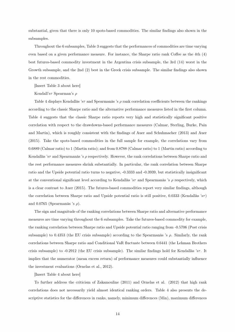
Table 1B. Descriptive statistics of daily excess returns - Argentina crisis



Aluminium -0.0241 0.0520 -3.54e-5 9.43e-3 0.8322 3.31 1.67

Copper -0.0308 0.0471 2.25e-4 0.0103 0.4731 1.44 1.06

Gold -0.0264 0.0272 5.71e-4 7.87e-3 -0.0162 1.45 2.03

Lead -0.0490 0.0304 -2.35e-4 0.0120 -0.1650 0.6284 1.03

Nickel -0.0645 0.0883 1.36e-3 0.0198 0.2042 1.48 0.8887

Palladium -0.0769 0.1285 -1.08e-3 0.0184 1.02 11.64 14.29**

Platinum -0.0396 0.0369 7.47e-4 0.0112 -0.4888 1.32 1.76

Silver -0.0399 0.0293 -2.31e-4 0.0107 -0.5641 1.10 2.15

Tin -0.0675 0.0298 1.44e-4 0.0121 -1.00 4.45 4.63*

Zinc -0.0353 0.0357 1.62e-4 0.0111 0.0831 1.13 3.13

Panel B. Futures Commodities

Brent -0.0663 0.0819 1.11e-3 0.0207 0.2431 1.45 2.29

Cocoa -0.0837 0.0563 8.87e-4 0.0168 -0.9908 5.50 16.29**

Coffee -0.0680 0.1042 1.89e-4 0.0245 0.3790 1.64 1.72

Corn -0.0697 0.0565 6.54e-4 0.0148 -0.1017 3.29 4.77*

Cotton -0.0868 0.0842 1.25e-3 0.0235 0.2091 1.39 2.35

Crude oil -0.0622 0.0995 1.24e-3 0.0221 0.1922 1.29 1.91

Gas -0.1967 0.1589 3.19e-3 0.0428 0.2385 2.55 3.66*

Gasoline -0.0881 0.0790 3.80e-4 0.0273 -0.3748 0.4472 3.99*

Heating oil -0.0800 0.0904 2.77e-4 0.0259 -0.3690 0.9578 6.80**

Oat -0.1707 0.0602 -3.89e-4 0.0245 -1.99 10.76 9.25**

Rice -0.0748 0.0764 6.66e-5 0.0193 0.0440 2.85 3.01

Rubber -0.0193 0.0269 2.06e-3 8.11e-3 0.1317 0.2361 1.35

Soybeans -0.0405 0.0510 7.83e-4 0.0129 -0.1040 1.16 1.39

Sugar -0.1266 0.0954 7.96e-4 0.0251 -0.1482 2.60 0.5554

Wheat -0.0464 0.0469 1.35e-3 0.0135 0.3283 1.08 2.33

Wool -0.1348 0.1326 1.96e-3 0.0178 1.01 28.53 89.69***

Notes. Table 1B reports the descriptive statistics (minimum, maximum, mean, standard deviation,

skewness, kurtosis and JB test statistic) of the daily excess returns of all commodities in theArgentinacrisis

subsample.

21

Table 1C. Descriptive statistics of daily excess returns - Growth


Panel A. Spot Commodities

Aluminium -0.0826 0.0531 4.36e-4 0.0141 -0.3964 2.83 6.25**

Copper -0.1036 0.1155 1.02e-3 0.0180 -0.1646 3.51 7.40**

Gold -0.0628 0.0406 6.41e-4 0.0113 -0.6684 2.86 11.05**

Lead -0.1015 0.1063 9.59e-4 0.0227 -0.1645 2.11 8.06**

Nickel -0.1836 0.1054 6.61e-4 0.0255 -0.2781 3.18 5.75**

Palladium -0.1242 0.1059 9.47e-5 0.0220 -0.4285 4.53 23.76***

Platinum -0.1027 0.0822 3.78e-4 0.0161 -0.6823 4.96 16.82**

Silver -0.1461 0.1081 6.82e-4 0.0231 -0.9210 5.63 18.80**

Tin -0.1145 0.1118 1.02e-3 0.0177 -0.4537 5.49 21.24***

Zinc -0.0980 0.0771 5.22e-4 0.0210 -0.2700 2.09 8.99**


Brent -0.0848 0.1030 1.00e-3 0.0204 0.0493 1.52 3.15

Cocoa -0.1928 0.1938 3.34e-4 0.0214 -0.5228 20.16 58.69***

Coffee -0.0879 0.1297 4.09e-4 0.0205 0.1210 2.29 5.70**

Corn -0.0722 0.0868 5.52e-4 0.0190 0.0591 1.27 6.25**

Cotton -0.0757 0.0893 1.87e-4 0.0190 -0.0493 1.89 9.86**

Crude oil -0.1225 0.0841 9.72e-4 0.0216 -0.3055 1.95 2.91

Gas -0.2392 0.2634 4.51e-4 0.0430 0.2401 5.13 17.71**

Gasoline -0.2487 0.1815 3.28e-4 0.0301 -0.2949 4.92 5.13**

Heating oil -0.0970 0.1032 3.84e-4 0.0225 -0.0360 1.70 10.42**

Oat -0.1127 0.0882 2.03e-4 0.0193 -0.2406 2.89 14.59**

Rice -0.2445 0.1618 1.02e-3 0.0184 -1.11 26.49 20.31***

Rubber -0.0387 0.0277 7.09e-4 7.55e-3 -0.5213 2.22 8.08**

Soybeans -0.1338 0.0761 2.88e-4 0.0190 -0.6471 3.86 9.73**

Sugar -0.1000 0.1685 4.35e-4 0.0214 0.1759 4.68 6.81**

Wheat -0.0811 0.0847 3.63e-4 0.0193 0.0849 1.91 8.52**

Wool -0.1117 0.1046 -2.11e-4 9.29e-3 -0.5970 60.91 246.30***

Notes. Table 1C reports the descriptive statistics (minimum, maximum, mean, standard deviation,

skewness, kurtosis and JB test statistic) of the daily excess returns of all commodities in the Growth

subsample.

22

Table 1D. Descriptive statistics of daily excess returns - Lehman Brothers



Aluminium -0.0755 0.0607 -2.01e-4 0.0193 -0.3583 0.7862 0.6167

Copper -0.1032 0.1173 2.79e-4 0.0263 -0.1810 1.68 2.55

Gold -0.0714 0.0687 8.95e-4 0.0149 0.0751 3.48 7.61**

Lead -0.1320 0.1301 3.19e-4 0.0318 -0.2987 1.43 1.39

Nickel -0.1374 0.1331 2.98e-4 0.0318 -0.0397 2.23 2.92

Palladium -0.1786 0.1092 1.56e-3 0.0281 -0.6653 4.56 5.58**

Platinum -0.0594 0.0464 7.49e-4 0.0133 -0.4025 1.83 1.69

Silver -0.1248 0.0597 2.05e-3 0.0220 -0.8719 3.03 3.87*

Tin -0.0994 0.1539 3.83e-4 0.0257 0.1149 3.81 6.37**

Zinc -0.1147 0.0961 4.20e-4 0.0282 -0.2330 0.7421 0.6167


Brent -0.1113 0.1350 -3.65e-4 0.0274 0.1842 2.59 3.36

Cocoa -0.0970 0.0880 1.53e-4 0.0204 -0.2236 3.03 8.38**

Coffee -0.0827 0.0594 1.39e-3 0.0185 -0.0116 1.01 1.34

Corn -0.1211 0.1089 2.04e-5 0.0266 -0.2656 2.60 5.96**

Cotton -0.0750 0.0904 1.19e-3 0.0242 -0.0636 1.21 4.96

Crude oil -0.1283 0.1641 -4.35e-4 0.0340 0.1278 3.55 8.13**

Gas -0.2553 0.2839 -1.03e-3 0.0471 0.8426 9.18 8.97**

Gasoline -0.1115 0.0676 1.10e-3 0.0206 -0.4810 1.97 2.27

Heating oil -0.0997 0.0891 1.46e-3 0.0201 -0.0029 4.48 13.96**

Oat -0.0866 0.1268 4.59e-4 0.0262 0.3695 2.53 5.87**

Rice -0.0602 0.0427 -4.88e-4 0.0170 -0.0512 -0.0114 1.01

Rubber -0.0579 0.0445 5.67e-4 0.0112 -1.63 7.87 23.04***

Soybeans -0.1341 0.0620 7.23e-4 0.0170 -0.9119 7.84 5.41**

Sugar -0.1166 0.1073 1.20e-3 0.0281 -0.3328 1.24 0.5195

Wheat -0.0995 0.1254 -6.59e-5 0.0278 0.2206 2.17 4.17*

Wool -0.0768 0.0523 2.82e-4 0.0091 -0.7876 19.18 105.01***

Notes. Table 1D reports the descriptive statistics (minimum, maximum, mean, standard deviation,

skewness, kurtosis and JB test statistic) of the daily excess returns of all commodities in the LehmanBrothers

subsample.

23

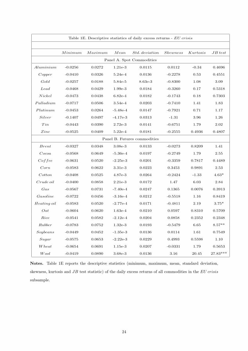
Table 1E. Descriptive statistics of daily excess returns - EU crisis



Aluminium -0.0256 0.0272 1.21e-3 0.0115 0.0112 -0.34 0.4696

Copper -0.0410 0.0326 5.24e-4 0.0136 -0.2278 0.53 0.4551

Gold -0.0257 0.0188 5.84e-5 8.63e-3 -0.8300 1.08 3.09

Lead -0.0468 0.0429 1.99e-3 0.0184 -0.3260 0.17 0.5318

Nickel -0.0473 0.0438 6.82e-4 0.0182 -0.1743 0.18 0.7303

Palladium -0.0717 0.0506 3.54e-4 0.0203 -0.7410 1.41 1.83

Platinum -0.0453 0.0264 -5.48e-4 0.0147 -0.7921 0.71 1.17

Silver -0.1407 0.0497 -4.17e-3 0.0313 -1.31 3.96 1.26

Tin -0.0443 0.0390 2.72e-3 0.0141 -0.6751 1.79 2.02

Zinc -0.0525 0.0409 5.22e-4 0.0181 -0.2555 0.4936 0.4807


Brent -0.0327 0.0348 3.08e-3 0.0133 -0.0273 0.8209 1.41

Cocoa -0.0568 0.0649 -5.36e-4 0.0197 -0.2749 1.79 2.55

Coffee -0.0631 0.0520 -2.25e-3 0.0201 -0.3359 0.7817 0.4489

Corn -0.0583 0.0622 3.31e-3 0.0223 0.3453 0.9891 2.53

Cotton -0.0408 0.0525 4.87e-3 0.0264 -0.2424 -1.33 4.63*

Crude oil -0.0400 0.0858 2.21e-3 0.0172 1.47 6.03 2.84

Gas -0.0567 0.0731 -7.40e-4 0.0247 0.1365 0.0076 0.3913

Gasoline -0.0722 0.0456 -3.16e-4 0.0212 -0.5518 1.16 0.8419

Heating oil -0.0583 0.0520 -2.77e-4 0.0171 -0.4811 2.19 3.75*

Oat -0.0604 0.0620 1.63e-4 0.0210 0.0597 0.8310 0.5709

Rice -0.0541 0.0582 -2.12e-4 0.0204 0.0858 0.2352 0.2348

Rubber -0.0783 0.0752 1.32e-3 0.0193 -0.5479 6.65 8.57**

Soybeans -0.0449 0.0452 -1.35e-3 0.0136 0.0114 1.61 0.7549

Sugar -0.0575 0.0653 -2.22e-3 0.0229 0.4993 0.5598 1.10

Wheat -0.0654 0.0691 1.15e-3 0.0207 -0.0331 1.79 0.5653

Wool -0.0419 0.0890 3.68e-3 0.0136 3.16 20.45 27.83***

Notes. Table 1E reports the descriptive statistics (minimum, maximum, mean, standard deviation,

skewness, kurtosis and JB test statistic) of the daily excess returns of all commodities in the EU crisis

subsample.

24

Table 1F. Descriptive statistics of daily excess returns - Greek crisis



Aluminium -0.0513 0.0580 -8.59e-4 0.0148 -0.0817 1.27 0.7005

Copper -0.0782 0.0668 -3.64e-4 0.0192 -0.0336 2.21 3.18

Gold -0.0587 0.0379 6.44e-4 0.0136 -0.9662 2.70 6.49**

Lead -0.0711 0.0741 -1.24e-3 0.0225 -0.0763 0.9728 1.70

Nickel -0.0775 0.0779 -1.39e-3 0.0223 -0.0434 1.02 1.42

Palladium -0.0857 0.0686 -7.23e-4 0.0216 -0.1754 1.59 1.51

Platinum -0.0361 0.0437 -2.11e-4 0.0131 0.1379 0.8292 1.35

Silver -0.0744 0.0698 8.34e-5 0.0184 0.1485 2.03 2.16

Tin -0.0878 0.0702 -1.27e-3 0.0218 -0.4453 1.78 3.70*

Zinc -0.0579 0.0585 -7.15e-4 0.0189 -0.1149 0.49 0.5393


Brent -0.0591 0.0378 2.19e-4 0.0157 -0.3666 0.95 1.66

Cocoa -0.0483 0.0758 -8.75e-4 0.0194 0.5386 1.44 3.96*

Coffee -0.0674 0.0646 -1.69e-3 0.0173 -0.0115 2.20 8.41**

Corn -0.0696 0.0643 -4.98e-4 0.0206 -0.3343 1.41 5.42**

Cotton -0.1024 0.1000 -3.03e-3 0.0231 -0.1096 2.20 3.84*

Crude oil -0.0853 0.0513 -8.27e-6 0.0201 -0.7217 2.09 4.11*

Gas -0.0787 0.0927 -2.87e-3 0.0273 0.3580 1.31 2.78

Gasoline -0.0720 0.0380 5.89e-5 0.0158 -0.6116 2.37 5.94**

Heating oil -0.0380 0.0458 2.39e-4 0.0118 0.2486 1.46 7.53**

Oat -0.0868 0.0750 -1.48e-4 0.0207 -0.0031 2.90 5.37**

Rice -0.0477 0.0644 2.29e-4 0.0158 0.4020 1.02 1.37

Rubber -0.0762 0.0433 -1.11e-3 0.0122 -1.04 6.81 9.24**

Soybeans -0.0483 0.0451 8.73e-4 0.0152 -0.0362 0.60 2.69

Sugar -0.0522 0.0678 -7.88e-4 0.0151 0.0671 2.18 0.1011

Wheat -0.1050 0.0653 -1.19e-3 0.0243 -0.4718 1.46 1.24

Wool -0.0420 0.0247 -5.10e-4 6.48e-3 -1.76 13.77 124.26***

Notes. Table 1F reports the descriptive statistics (minimum, maximum, mean, standard deviation,

skewness, kurtosis and JB test statistic) of the daily excess returns of all commodities in the Greekcrisis

subsample.

25

Table 1G. Descriptive statistics of daily excess returns - Post debt crisis



Aluminium -0.0357 0.0459 -2.43e-5 0.0114 0.3771 0.8843 0.7646

Copper -0.0394 0.0606 -2.84e-4 0.0111 0.1265 2.38 3.73*

Gold -0.1016 0.0543 -4.20e-4 0.0109 -1.44 13.98 10.05**

Lead -0.0311 0.0520 1.60e-4 0.0123 0.2316 0.8551 0.6091

Nickel -0.0658 0.0602 8.04e-5 0.0150 0.1086 1.25 1.08

Palladium -0.0568 0.0530 4.88e-4 0.0134 -0.2915 2.10 3.67*

Platinum -0.0446 0.0439 -4.03e-4 0.0100 0.0173 1.58 1.83

Silver -0.1518 0.0688 -6.37e-4 0.0148 -1.78 19.78 12.51**

Tin -0.0594 0.0639 -4.69e-5 0.0135 0.0671 3.27 7.22**

Zinc -0.0321 0.0461 2.60e-4 0.0112 0.1694 0.5265 0.5550


Brent -0.0462 0.0474 -3.58e-4 0.0113 -0.2288 1.84 2.24

Cocoa -0.0477 0.0367 4.81e-4 0.0122 -0.0148 0.9295 3.31

Coffee -0.2324 0.2257 1.86e-4 0.0290 0.8043 28.07 35.24***

Corn -0.0869 0.0667 -8.68e-4 0.0166 -0.2523 3.45 5.58**

Cotton -0.0995 0.0833 -4.81e-4 0.0163 -0.4638 4.37 7.97**

Crude oil -0.0599 0.0900 -2.06e-4 0.0135 0.1272 4.48 3.73*

Gas -0.2702 0.3781 1.05e-3 0.0399 1.34 29.28 27.89***

Gasoline -0.0762 0.2441 -1.05e-3 0.0189 3.80 48.72 30.74***

Heating oil -0.0553 0.0931 -8.31e-4 0.0116 0.3651 9.42 21.84***

Oat -0.2450 0.2371 1.00e-4 0.0294 -0.9327 28.36 28.55***

Rice -0.1109 0.0512 -2.25e-4 0.0118 -1.31 13.19 2.95

Rubber -0.0434 0.0337 -1.24e-3 0.0111 -0.4704 1.35 5.48**

Soybeans -0.1096 0.0761 -6.05e-4 0.0146 -1.41 11.43 10.06**

Sugar -0.0399 0.1419 -2.99e-4 0.0127 2.51 25.58 10.27**

Wheat -0.2011 0.2259 -2.95e-4 0.0281 0.2401 17.83 20.26***

Wool -0.0460 0.0491 -3.06e-4 0.0078 0.0626 13.33 97.59***

Notes. Table 1G reports the descriptive statistics (minimum, maximum, mean, standard deviation,

skewness, kurtosis and JB test statistic) of the daily excess returns of all commodities in the Postdebtcrisis

subsample.

26

Table 2. Performance measures

No. Performance measure Original proposal Reward measure Risk measure

Classic

1 Sharpe ratio Sharpe (1966) µ σ

Based on drawdowns

2 Calmar ratio Young (1991) µ MDD

3 Sterling ratio Kestner (1996) µ K−1∑Kk=1 CDDk

4 Burke ratio Burke (1994) µ[∑K

k=1 CDD2k

]1/25 Pain ratio Zephyr Associates (2006) µ T−1

∑Tt=1DDPt

6 Martin ratio Martin and McCann (1998) µ[T−1

∑Tt=1DDP

2t

]1/2Based on partial moments

7 Omega ratio Keating and Shadwick (2002) µ LPM1

8 Sortino ratio Sortino and van der Meer (1991) µ [LPM2]1/2

9 Kappa3 ratio Kaplan and Knowles (2004) µ [LPM3]1/3

10 Upside potential ratio Sortino et al. (1999) HPM1 [LPM2]1/2

Based on Value at Risk (VaR)

11 Excess return on V aR Dowd (2000) µ V aRa

12 Conditional Sharpe ratio Agarwal and Naik (2004) µ CV aRa

13 Modified Sharpe ratio Gregoriou and Gueyie (2003) µ MV aRa

Notes. Table 2 presents the investment performance measures applied in our study. µ = T−1 (R1 + · · ·+RT )

and σ =[T−1

{(R1 − µ)

2+ · · ·+ (RT − µ)

2}]1/2

are the mean and the standard deviation of the ex-

cess returns Rt = rt − rf,t, t = 1, ..., T of a given commodity. rt = lnPt − lnPt−1 is the daily

natural log return, Pt is the daily commodity price. MDD denotes for the largest negative cumu-

lative excess return; CDDk is the k-th largest negative cumulative excess return that is not inter-

rupted by a positive excess return; DDPk denotes a negative cumulative excess return from the pre-

vious peak. k is the number of continuous drawdowns incorporated in the calculation. The signs of

the drawdowns are dropped to generate positive risk measures. HPMm=T−1∑Tt=1max (Rt, 0)

m and

LPMm=T−1∑Tt=1max (−Rt, 0)

m are higher and lower partial moments of order m. V aRa denotes

for the Value at Risk (VaR) at the a-quantile of the excess return distribution; V aRa= − (µ+ σza).

The conditional VaR is estimated as CV aRa=B−1∑Rt≤−V aRa

−Rt, B is the number of excess re-

turns fulfilling the summation condition. The modified VaR (MV aRa) is estimated as MV aRa= −[µ+ σ

{za +

(z2a − 1

)γ/6 +

(z3a − 3za

)k/24−

(2z3a − 5za

)γ2/36

}], where za is the a-quantile of the

standard normal distribution, γ and κ denote skewness and excess kurtosis of the excess return dis-

tribution (Auer, 2015).

27

Table 3A. Investment rankings - Full sample

Classic Based-on-drawdowns Based-on-partial-moments Based-on-the-Value-at-Risk

Sample Sharpe Calmar Sterling Burke Pain Martin Omega Sortino Kappa3 Upside Excess Conditional Modified Mean


Aluminium 10 9 10 10 10 10 10 10 10 9 10 8 8 8

Copper 3 1 2 2 4 3 4 2 2 6 4 9 9 9

Gold 1 2 1 1 1 1 1 1 1 10 1 1 1 1

Lead 6 6 6 6 6 6 6 6 6 2 6 2 2 2

Nickel 7 5 7 7 7 7 7 5 5 1 5 4 4 4

Palladium 8 8 8 8 8 8 8 8 8 3 9 3 3 3

Platinum 2 4 3 3 3 2 2 7 7 8 2 5 5 5

Silver 5 7 5 5 5 5 5 4 4 4 3 7 7 7

Tin 4 3 4 4 2 4 3 3 3 7 7 10 10 10

Zinc 9 10 9 9 9 9 9 9 9 5 8 6 6 6


Brent 1 1 1 1 2 1 2 1 1 4 1 1 1 1

Crude oil 10 11 8 9 9 11 9 10 10 12 11 12 12 12

Gas 15 13 13 13 15 13 15 14 14 7 14 9 9 9

Gasoline 8 4 10 8 8 8 8 8 8 11 6 3 3 3

Heat oil 16 16 16 16 16 16 16 16 16 10 15 10 10 10

Cocoa 2 2 3 2 4 3 4 2 2 3 3 2 2 2

Coffee 14 14 15 14 13 14 14 13 12 1 13 16 16 15

Corn 7 5 7 7 7 7 7 5 4 2 7 4 4 4

Cotton 4 3 4 3 3 4 5 3 3 5 2 7 7 7

Oat 6 7 5 6 6 6 6 4 5 6 8 8 8 8

Rice 13 15 14 15 14 15 13 15 15 13 16 13 13 16

Rubber 3 6 6 5 5 2 3 7 7 15 4 5 5 5

Soybeans 9 9 9 10 10 9 10 12 13 14 5 11 11 11

Sugar 12 12 12 12 12 12 12 11 11 8 10 14 14 14

Wheat 11 10 11 11 11 10 11 9 9 9 12 15 15 13

Wool 5 8 2 4 1 5 1 6 6 16 9 6 6 6

Notes. Table 3A reports the investment rankings of the Spot and Futures commodities in the Full

sample.

28

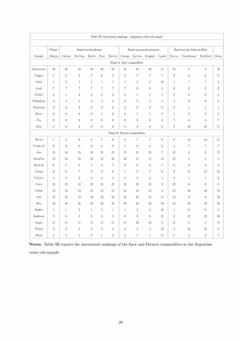
Table 3B. Investment rankings - Argentina crisis sub-sample




Aluminium 10 10 10 10 10 10 10 10 10 9 10 5 5 10

Copper 5 5 5 5 6 5 5 7 7 7 8 6 6 8

Gold 1 3 1 1 1 1 1 4 4 10 1 7 7 3

Lead 7 7 7 7 7 7 7 6 6 5 6 2 2 2

Nickel 2 1 2 2 2 3 2 1 1 1 3 8 8 4

Palladium 4 4 4 4 4 4 4 2 2 2 4 9 9 6

Platinum 3 2 3 3 3 2 3 3 3 3 2 1 1 1

Silver 6 6 6 6 5 6 6 5 5 8 5 3 3 5

Tin 9 9 9 9 9 9 9 9 9 4 7 4 4 7

Zinc 8 8 8 8 8 8 8 8 8 6 9 10 10 9


Brent 7 3 6 6 7 6 8 7 7 8 8 14 14 11

Crude oil 9 9 9 9 6 9 5 8 8 11 4 7 7 7

Gas 15 14 15 15 15 15 15 15 15 7 15 8 9 15

Gasoline 10 10 10 10 10 10 10 11 11 14 10 4 4 4

Heat oil 8 7 8 7 8 7 9 6 6 5 6 3 3 3

Cocoa 6 8 7 8 9 8 7 5 5 6 9 15 15 12

Coffee 4 4 4 4 4 4 4 3 2 1 3 1 1 2

Corn 13 12 12 12 12 12 13 13 13 2 13 6 6 8

Cotton 14 13 14 14 14 14 14 14 14 3 14 16 16 14

Oat 12 15 13 13 13 13 12 12 12 9 12 9 8 13

Rice 16 16 16 16 16 16 16 16 16 10 16 10 10 16

Rubber 1 1 2 1 2 1 1 2 3 16 1 11 11 5

Soybeans 5 6 5 5 5 5 6 9 9 15 5 12 12 10

Sugar 11 11 11 11 11 11 11 10 10 4 11 5 5 6

Wheat 3 2 3 3 3 3 3 4 4 13 2 13 13 9

Wool 2 5 1 2 1 2 2 1 1 12 7 2 2 1

Notes. Table 3B reports the investment rankings of the Spot and Futures commodities in the Argentina

crisis sub-sample.

29

Table 3C. Investment rankings - Growth sub-sample




Aluminium 5 5 5 5 5 5 5 8 8 9 5 7 7 7

Copper 3 1 1 1 3 1 3 2 2 6 4 9 9 8

Gold 2 2 3 3 2 2 2 4 4 10 1 3 3 2

Lead 4 4 4 4 4 4 4 3 3 2 3 10 10 10

Nickel 7 8 8 7 8 7 7 6 6 1 8 2 2 3

Palladium 10 10 10 10 10 10 10 10 10 5 10 8 8 9

Platinum 9 9 9 9 9 9 9 9 9 8 9 4 4 4

Silver 6 6 6 6 6 6 6 5 5 3 7 6 6 6

Tin 1 3 2 2 1 3 1 1 1 7 2 1 1 1

Zinc 8 7 7 8 7 8 8 7 7 4 6 5 5 5


Brent 3 2 3 3 3 3 3 2 2 5 3 14 14 8

Crude oil 11 11 8 10 7 11 8 10 10 14 15 8 8 12

Gas 8 7 7 8 9 8 9 7 8 7 9 9 9 11

Gasoline 5 4 6 5 6 5 6 5 5 8 4 10 10 9

Heat oil 16 14 16 16 16 16 16 16 16 13 12 11 11 16

Cocoa 4 3 4 4 4 4 4 4 3 3 2 3 3 3

Coffee 14 16 14 15 15 15 13 9 7 1 16 15 15 15

Corn 13 15 13 13 13 13 15 13 13 2 14 4 4 4

Cotton 10 6 10 11 10 10 11 8 9 4 8 16 16 13

Oat 15 12 15 14 14 14 14 15 15 11 11 7 7 7

Rice 2 5 1 2 2 2 2 1 1 12 5 1 1 1

Rubber 1 1 2 1 1 1 1 3 4 15 1 2 2 2

Soybeans 12 9 12 12 12 12 12 14 14 10 7 5 5 5

Sugar 7 8 9 7 8 7 7 6 6 6 10 12 12 10

Wheat 9 10 11 9 11 9 10 12 11 9 6 13 13 14

Wool 6 13 5 6 5 6 5 11 12 16 13 6 6 6

Notes. Table 3C reports the investment rankings of the Spot and Futures commodities in the Growth

sub-sample.

30

Table 3D. Investment rankings - Lehman Brothers sub-sample




Aluminium 8 6 10 8 8 8 9 10 10 8 6 8 8 8

Copper 7 8 7 7 7 7 7 9 9 6 9 9 9 10

Gold 2 2 2 2 2 2 2 3 3 9 4 1 1 1

Lead 9 9 9 9 9 9 8 7 7 1 8 6 6 6

Nickel 10 10 8 10 10 10 10 8 8 2 10 7 7 7

Palladium 4 3 3 3 3 4 3 2 2 3 3 4 4 4

Platinum 3 4 4 4 4 3 4 4 4 10 2 2 2 2

Silver 1 1 1 1 1 1 1 1 1 5 1 3 3 3

Tin 5 5 5 6 5 5 5 6 6 7 7 10 10 9

Zinc 6 7 6 5 6 6 6 5 5 4 5 5 5 5


Brent 12 12 13 12 13 12 13 13 13 7 12 14 14 14

Crude oil 14 14 14 14 14 14 14 14 14 12 14 8 8 9

Gas 1 2 2 2 2 2 2 2 2 11 1 3 3 3

Gasoline 16 16 16 16 16 16 16 16 16 8 16 10 10 15

Heat oil 5 3 3 4 5 5 6 3 3 4 4 11 11 10

Cocoa 13 13 12 13 12 13 12 12 12 3 13 15 15 13

Coffee 10 11 10 10 10 10 10 6 6 1 10 16 16 11

Corn 3 4 4 3 4 4 5 4 4 9 3 5 5 5

Cotton 2 1 1 1 1 1 1 1 1 10 2 1 1 1

Oat 11 9 11 11 11 11 11 11 11 6 11 12 12 12

Rice 9 7 9 9 9 9 9 10 10 14 7 4 4 4

Rubber 4 6 8 8 6 3 3 8 8 15 5 9 9 8

Soybeans 6 8 7 6 7 6 7 7 7 13 6 6 6 6

Sugar 7 5 6 5 8 7 8 5 5 2 8 2 2 2

Wheat 15 15 15 15 15 15 15 15 15 5 15 13 13 16

Wool 8 10 5 7 3 8 4 9 9 16 9 7 7 7

Notes. Table 3D reports the investment rankings of the Spot and Futures commodities in the Lehman

Brothers sub-sample.

31

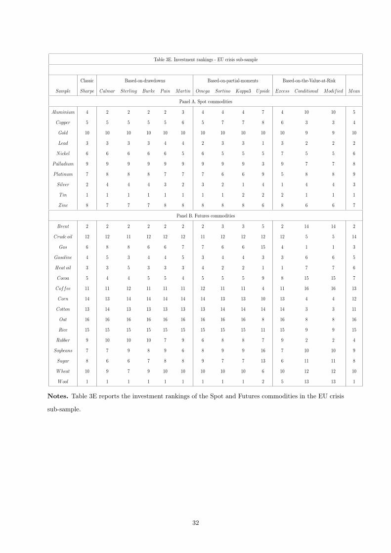
Table 3E. Investment rankings - EU crisis sub-sample




Aluminium 4 2 2 2 2 3 4 4 4 7 4 10 10 5

Copper 5 5 5 5 5 6 5 7 7 8 6 3 3 4

Gold 10 10 10 10 10 10 10 10 10 10 10 9 9 10

Lead 3 3 3 3 4 4 2 3 3 1 3 2 2 2

Nickel 6 6 6 6 6 5 6 5 5 5 7 5 5 6

Palladium 9 9 9 9 9 9 9 9 9 3 9 7 7 8

Platinum 7 8 8 8 7 7 7 6 6 9 5 8 8 9

Silver 2 4 4 4 3 2 3 2 1 4 1 4 4 3

Tin 1 1 1 1 1 1 1 1 2 2 2 1 1 1

Zinc 8 7 7 7 8 8 8 8 8 6 8 6 6 7


Brent 2 2 2 2 2 2 2 3 3 5 2 14 14 2

Crude oil 12 12 11 12 12 12 11 12 12 12 12 5 5 14

Gas 6 8 8 6 6 7 7 6 6 15 4 1 1 3

Gasoline 4 5 3 4 4 5 3 4 4 3 3 6 6 5

Heat oil 3 3 5 3 3 3 4 2 2 1 1 7 7 6

Cocoa 5 4 4 5 5 4 5 5 5 9 8 15 15 7

Coffee 11 11 12 11 11 11 12 11 11 4 11 16 16 13

Corn 14 13 14 14 14 14 14 13 13 10 13 4 4 12

Cotton 13 14 13 13 13 13 13 14 14 14 14 3 3 11

Oat 16 16 16 16 16 16 16 16 16 8 16 8 8 16

Rice 15 15 15 15 15 15 15 15 15 11 15 9 9 15

Rubber 9 10 10 10 7 9 6 8 8 7 9 2 2 4

Soybeans 7 7 9 8 9 6 8 9 9 16 7 10 10 9

Sugar 8 6 6 7 8 8 9 7 7 13 6 11 11 8

Wheat 10 9 7 9 10 10 10 10 10 6 10 12 12 10

Wool 1 1 1 1 1 1 1 1 1 2 5 13 13 1

Notes. Table 3E reports the investment rankings of the Spot and Futures commodities in the EU crisis

sub-sample.

32

Table 3F. Investment rankings - Greek crisis sub-sample




Aluminium 3 1 2 2 3 2 4 4 4 9 5 6 6 6

Copper 8 9 8 8 8 8 8 8 8 7 8 4 4 4

Gold 5 6 1 5 4 5 3 5 5 8 3 3 3 3

Lead 4 3 5 4 5 4 5 3 3 1 4 7 7 7

Nickel 1 2 3 1 2 1 1 1 1 3 2 8 8 5

Palladium 7 5 6 7 7 7 7 7 7 2 7 2 2 2

Platinum 9 8 9 9 9 9 9 9 9 10 9 9 9 10

Silver 10 10 10 10 10 10 10 10 10 5 10 5 5 8

Tin 2 4 4 3 1 3 2 2 2 4 1 1 1 1

Zinc 6 7 7 6 6 6 6 6 6 6 6 10 10 9


Brent 13 12 12 13 13 13 13 13 13 8 11 9 9 12

Crude oil 9 5 9 9 9 9 9 8 8 7 9 12 12 11

Gas 3 1 2 2 3 3 4 3 3 14 3 3 3 3

Gasoline 10 10 10 10 10 10 10 10 10 4 10 7 7 7

Heat oil 1 3 3 1 2 1 2 1 1 10 2 1 1 1

Cocoa 16 16 16 16 16 16 16 16 16 2 16 11 11 16

Coffee 2 2 4 3 4 2 3 2 2 3 1 15 15 8

Corn 15 15 15 15 15 15 15 15 15 11 15 10 10 15

Cotton 11 11 11 11 11 11 11 11 11 13 12 16 16 13

Oat 14 14 14 14 14 14 14 14 14 5 14 8 8 9

Rice 12 13 13 12 12 12 12 12 12 9 13 13 13 14

Rubber 4 9 5 5 5 4 5 4 4 15 4 4 4 4

Soybeans 6 7 6 6 6 6 6 7 7 6 6 2 2 2

Sugar 7 6 7 8 8 8 7 9 9 12 8 14 14 10

Wheat 8 4 8 7 7 7 8 6 5 1 7 5 5 6

Wool 5 8 1 4 1 5 1 5 6 16 5 6 6 5

Notes. Table 3F reports the investment rankings of the Spot and Futures commodities in the Greek

sub-sample.

33

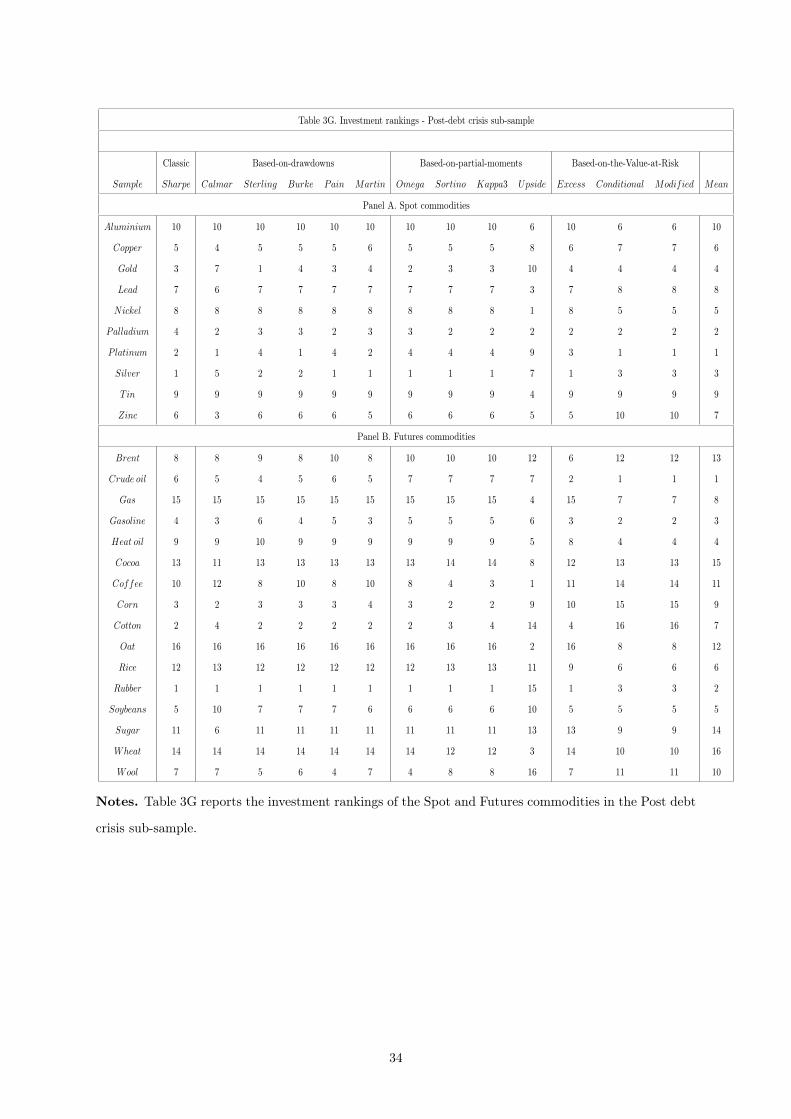
Table 3G. Investment rankings - Post-debt crisis sub-sample




Aluminium 10 10 10 10 10 10 10 10 10 6 10 6 6 10

Copper 5 4 5 5 5 6 5 5 5 8 6 7 7 6

Gold 3 7 1 4 3 4 2 3 3 10 4 4 4 4

Lead 7 6 7 7 7 7 7 7 7 3 7 8 8 8

Nickel 8 8 8 8 8 8 8 8 8 1 8 5 5 5

Palladium 4 2 3 3 2 3 3 2 2 2 2 2 2 2

Platinum 2 1 4 1 4 2 4 4 4 9 3 1 1 1

Silver 1 5 2 2 1 1 1 1 1 7 1 3 3 3

Tin 9 9 9 9 9 9 9 9 9 4 9 9 9 9

Zinc 6 3 6 6 6 5 6 6 6 5 5 10 10 7


Brent 8 8 9 8 10 8 10 10 10 12 6 12 12 13

Crude oil 6 5 4 5 6 5 7 7 7 7 2 1 1 1

Gas 15 15 15 15 15 15 15 15 15 4 15 7 7 8

Gasoline 4 3 6 4 5 3 5 5 5 6 3 2 2 3

Heat oil 9 9 10 9 9 9 9 9 9 5 8 4 4 4

Cocoa 13 11 13 13 13 13 13 14 14 8 12 13 13 15

Coffee 10 12 8 10 8 10 8 4 3 1 11 14 14 11

Corn 3 2 3 3 3 4 3 2 2 9 10 15 15 9

Cotton 2 4 2 2 2 2 2 3 4 14 4 16 16 7

Oat 16 16 16 16 16 16 16 16 16 2 16 8 8 12

Rice 12 13 12 12 12 12 12 13 13 11 9 6 6 6

Rubber 1 1 1 1 1 1 1 1 1 15 1 3 3 2

Soybeans 5 10 7 7 7 6 6 6 6 10 5 5 5 5

Sugar 11 6 11 11 11 11 11 11 11 13 13 9 9 14

Wheat 14 14 14 14 14 14 14 12 12 3 14 10 10 16

Wool 7 7 5 6 4 7 4 8 8 16 7 11 11 10

Notes. Table 3G reports the investment rankings of the Spot and Futures commodities in the Post debt

crisis sub-sample.

34

Table 4A. Rank correlations and corresponding ranking difference statistics; Full sample

Rank correlations Ranking differences

τ p Min Max MAD SDAD

Spot Futures Spot Futures Spot Futures Spot Futures Spot Futures Spot Futures

Based-on-drawdowns Calmar 0.6889 0.7833 0.8788 0.9265 -2 -4 2 3 1.20 1.25 0.7888 1.29

Sterling 0.9556 0.8333 0.9879 0.9500 -1 -3 1 3 0.2000 1.00 0.4216 1.10

Burke 0.9556 0.9000 0.9879 0.9765 -1 -2 1 2 0.2000 0.6250 0.4216 0.8062

Pain 0.9111 0.8667 0.9636 0.9559 -2 -4 1 2 0.4000 0.8750 0.6992 1.09

Martin 1.00 0.9167 1.00 0.9824 0 -2 0 2 0 0.5000 0 0.7303

Based-on-partial-moments Omega 0.9556 0.9000 0.9879 0.9647 -1 -4 1 2 0.2000 0.6250 0.4216 1.09

Sortino 0.7333 0.8000 0.8061 0.9324 -2 -2 5 4 1.00 1.25 1.56 1.18

Kappa3 0.7333 0.7667 0.8061 0.9147 -2 -3 5 4 1.00 1.38 1.56 1.36

Upside -0.3333 0.0333 -0.3939 0.0765 -6 -13 9 12 4.20 4.75 2.44 4.22

Based-on-the-Value-at-Risk Excess 0.7333 0.7167 0.8788 0.9059 -2 -4 3 4 1.00 1.63 1.05 1.20

Conditional 0.1111 0.5833 0.1030 0.7706 -5 -6 6 4 3.40 2.50 1.90 1.93

Modified 0.1111 0.5833 0.1030 0.7706 -5 -6 6 4 3.40 2.50 1.90 1.93

Mean - - - - -5 -6 6 3 3.40 2.50 1.90 1.83

Notes. Table 4A reports the Kendall’s (τ) and Spearman’s (p) correlations between rankings for spot and

futures commodities in the Full sample. The table also provides descriptive statistics of the differences

in rankings.

35

Table 4B. Rank correlations and corresponding ranking difference statistics; Argentina crisis





Sterling 1.00 0.9500 1.00 0.9912 0 -1 0 1 0 0.3750 0 0.5000

Burke 1.00 0.9500 1.00 0.9882 0 -1 0 2 0 0.3750 0 0.6191

Pain 0.9556 0.8833 0.9879 0.9676 -1 -3 1 3 0.2000 0.6250 0.4216 1.02

Martin 0.9556 0.9500 0.9879 0.9882 -1 -1 1 2 0.2000 0.3750 0.4216 0.6191

Based-on-partial-moments Omega 1.00 0.9333 1.00 0.9706 0 -4 0 1 0 0.5000 0 1.03

Sortino 0.7333 0.8667 0.8788 0.9588 -2 -2 3 4 1.00 0.8750 1.05 1.02

Kappa3 0.7333 0.8500 0.8788 0.9588 -2 -2 3 4 1.00 1.00 1.05 1.10

Upside 0.2000 -0.2833 0.2242 -0.4176 -5 -11 9 15 2.60 6.50 2.59 4.38


Conditional -0.0667 0.1167 0.8909 0.0647 -5 -7 6 10 4.00 5.63 1.83 2.94

Modified -0.0667 0.1333 -0.1515 0.0735 -5 -7 6 10 4.00 5.63 1.83 2.87

Mean - - - - -5 -6 3 6 2.00 3.25 1.33 2.32

Notes. Table 4B reports the Kendall’s (τ) and Spearman’s (p) correlations between rankings for spot

and futures commodities in the Argentina crisis subsample. The table also provides descriptive statistics

of the differences in rankings.

36

Table 4C. Rank correlations and corresponding ranking difference statistics; Growth





Sterling 0.8667 0.8833 0.9515 0.9676 -2 -3 1 2 0.6000 0.7500 0.6992 0.9309

Burke 0.9111 0.9667 0.9636 0.9941 -2 -1 1 1 0.4000 0.2500 0.6992 0.4472

Pain 0.9556 0.8833 0.9879 0.9618 -1 -4 1 2 0.2000 0.7500 0.4216 1.06

Martin 0.8667 0.9833 0.9515 0.9971 -2 -1 2 1 0.4000 0.1250 0.8433 0.3416

Based-on-partial-moments Omega 1.00 0.9000 1.00 0.9706 0 -3 0 2 0 0.7500 0 0.8563

Sortino 0.7778 0.7667 0.8909 0.8882 -1 -5 3 5 1.00 1.50 0.9428 1.63

Kappa3 0.7778 0.7000 0.8909 0.8412 -1 -7 3 6 1.00 1.63 0.9428 2.09

Upside -0.2000 -0.0833 -0.3091 -0.1412 -6 -13 8 14 4.20 5.25 2.10 4.73


Conditional 0.0667 0.2167 0.1515 0.3294 -5 -9 6 11 3.00 4.25 2.36 3.34

Modified 0.0667 0.2167 0.1515 0.3294 -5 -9 6 11 3.00 4.25 2.36 3.34

Mean - - - - -5 -9 6 5 2.60 3.25 2.32 2.86

Notes. Table 4C reports the Kendall’s (τ) and Spearman’s (p) correlations between rankings for spot

and futures commodities in the Growth subsample. The table also provides descriptive statistics of the

differences in rankings.

37

Table 4D. Rank correlations and corresponding ranking difference statistics; Lehman Brothers





Sterling 0.8222 0.8333 0.9394 0.9471 -2 -3 2 4 0.6000 1.00 0.8433 1.15

Burke 0.9111 0.9000 0.9758 0.9647 -1 -2 1 4 0.4000 0.6250 0.5164 1.09

Pain 0.9556 0.8667 0.9879 0.9471 -1 -5 1 2 0.2000 0.8750 0.4216 1.26

Martin 1.00 0.9667 1.00 0.9941 0 -1 0 1 0 0.2500 0 0.4472


Sortino 0.6889 0.8167 0.8545 0.9294 -2 -4 2 4 1.40 1.25 0.6992 1.24

Kappa3 0.6889 0.8167 0.8545 0.9294 -2 -4 2 4 1.40 1.25 0.6992 1.24

Upside -0.3333 -0.1833 -0.5273 -0.3000 -8 -10 7 11 4.00 6.88 3.20 2.92


Conditional 0.4667 0.4500 0.6727 0.6441 -3 -6 5 6 1.80 3.25 1.55 2.21

Modified 0.4667 0.4500 0.6727 0.6441 -3 -6 5 6 1.80 3.25 1.55 2.21

Mean - - - - -3 -5 4 5 1.80 2.25 1.40 1.88

Notes. Table 4D reports the Kendall’s (τ) and Spearman’s (p) correlations between rankings for spot

and futures commodities in the Lehman Brothers subsample. The table also provides descriptive statistics


38

Table 4E. Rank correlations and corresponding ranking difference statistics; EU crisis





Sterling 0.8222 0.8667 0.9394 0.9559 -2 -3 2 2 0.6000 1.00 0.8433 0.9661

Burke 0.8222 0.9667 0.9394 0.9941 -2 -1 2 1 0.6000 0.2500 0.8433 0.4472

Pain 0.9111 0.9500 0.9636 0.9882 -2 -2 1 2 0.4000 0.2500 0.6992 0.6831

Martin 0.9111 0.9667 0.9758 0.9941 -1 -1 1 1 0.4000 0.2500 0.5164 0.4472


Sortino 0.9111 0.9333 0.9636 0.9853 -1 -1 2 2 0.4000 0.5000 0.6992 0.6325

Kappa3 0.8667 0.9333 0.9515 0.9853 -1 -1 2 2 0.6000 0.5000 0.6992 0.6325

Upside 0.4222 0.2667 0.5636 0.4353 -6 -8 3 9 2.20 4.00 1.62 2.92


Conditional 0.5556 -0.1667 0.6606 -0.2912 -2 -10 6 12 1.80 6.63 1.62 3.42

Modified 0.5556 -0.1667 0.6606 -0.2912 -2 -10 6 12 1.80 6.63 1.62 3.42

Mean - - - - -1 -5 2 3 0.8000 1.50 0.6325 1.46

Notes. Table 4E reports the Kendall’s (τ) and Spearman’s (p) correlations between rankings for spot

and futures commodities in the EU crisis subsample. The table also provides descriptive statistics of the

differences in rankings.

39

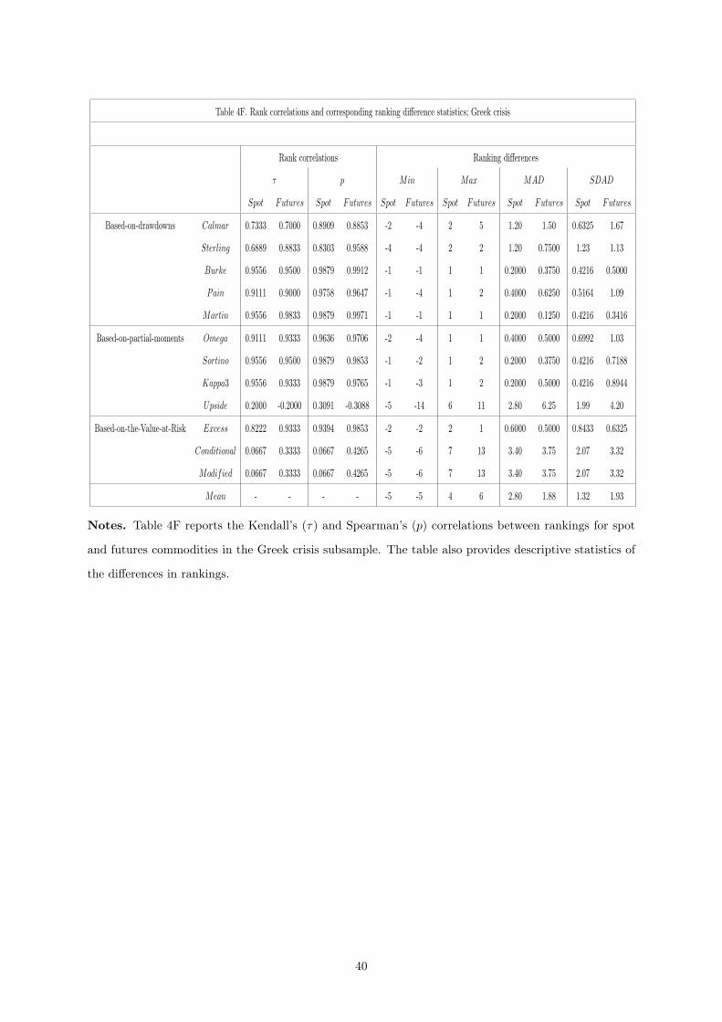
Table 4F. Rank correlations and corresponding ranking difference statistics; Greek crisis





Sterling 0.6889 0.8833 0.8303 0.9588 -4 -4 2 2 1.20 0.7500 1.23 1.13

Burke 0.9556 0.9500 0.9879 0.9912 -1 -1 1 1 0.2000 0.3750 0.4216 0.5000

Pain 0.9111 0.9000 0.9758 0.9647 -1 -4 1 2 0.4000 0.6250 0.5164 1.09

Martin 0.9556 0.9833 0.9879 0.9971 -1 -1 1 1 0.2000 0.1250 0.4216 0.3416


Sortino 0.9556 0.9500 0.9879 0.9853 -1 -2 1 2 0.2000 0.3750 0.4216 0.7188

Kappa3 0.9556 0.9333 0.9879 0.9765 -1 -3 1 2 0.2000 0.5000 0.4216 0.8944

Upside 0.2000 -0.2000 0.3091 -0.3088 -5 -14 6 11 2.80 6.25 1.99 4.20


Conditional 0.0667 0.3333 0.0667 0.4265 -5 -6 7 13 3.40 3.75 2.07 3.32

Modified 0.0667 0.3333 0.0667 0.4265 -5 -6 7 13 3.40 3.75 2.07 3.32

Mean - - - - -5 -5 4 6 2.80 1.88 1.32 1.93

Notes. Table 4F reports the Kendall’s (τ) and Spearman’s (p) correlations between rankings for spot

and futures commodities in the Greek crisis subsample. The table also provides descriptive statistics of

the differences in rankings.

40

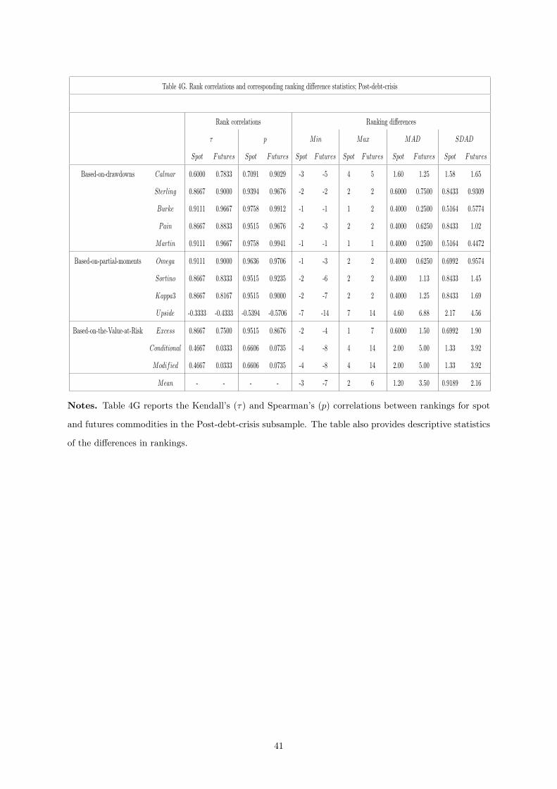
Table 4G. Rank correlations and corresponding ranking difference statistics; Post-debt-crisis





Sterling 0.8667 0.9000 0.9394 0.9676 -2 -2 2 2 0.6000 0.7500 0.8433 0.9309

Burke 0.9111 0.9667 0.9758 0.9912 -1 -1 1 2 0.4000 0.2500 0.5164 0.5774

Pain 0.8667 0.8833 0.9515 0.9676 -2 -3 2 2 0.4000 0.6250 0.8433 1.02

Martin 0.9111 0.9667 0.9758 0.9941 -1 -1 1 1 0.4000 0.2500 0.5164 0.4472


Sortino 0.8667 0.8333 0.9515 0.9235 -2 -6 2 2 0.4000 1.13 0.8433 1.45

Kappa3 0.8667 0.8167 0.9515 0.9000 -2 -7 2 2 0.4000 1.25 0.8433 1.69

Upside -0.3333 -0.4333 -0.5394 -0.5706 -7 -14 7 14 4.60 6.88 2.17 4.56


Conditional 0.4667 0.0333 0.6606 0.0735 -4 -8 4 14 2.00 5.00 1.33 3.92

Modified 0.4667 0.0333 0.6606 0.0735 -4 -8 4 14 2.00 5.00 1.33 3.92

Mean - - - - -3 -7 2 6 1.20 3.50 0.9189 2.16

Notes. Table 4G reports the Kendall’s (τ) and Spearman’s (p) correlations between rankings for spot

and futures commodities in the Post-debt-crisis subsample. The table also provides descriptive statistics


41

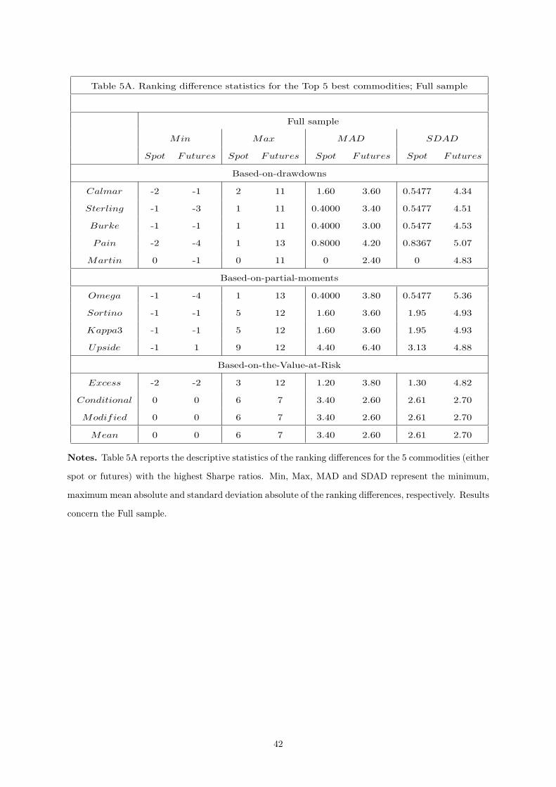
Table 5A. Ranking difference statistics for the Top 5 best commodities; Full sample

Full sample

Min Max MAD SDAD

Spot Futures Spot Futures Spot Futures Spot Futures

Based-on-drawdowns

Calmar -2 -1 2 11 1.60 3.60 0.5477 4.34

Sterling -1 -3 1 11 0.4000 3.40 0.5477 4.51

Burke -1 -1 1 11 0.4000 3.00 0.5477 4.53

Pain -2 -4 1 13 0.8000 4.20 0.8367 5.07

Martin 0 -1 0 11 0 2.40 0 4.83

Based-on-partial-moments

Omega -1 -4 1 13 0.4000 3.80 0.5477 5.36

Sortino -1 -1 5 12 1.60 3.60 1.95 4.93

Kappa3 -1 -1 5 12 1.60 3.60 1.95 4.93

Upside -1 1 9 12 4.40 6.40 3.13 4.88

Based-on-the-Value-at-Risk

Excess -2 -2 3 12 1.20 3.80 1.30 4.82

Conditional 0 0 6 7 3.40 2.60 2.61 2.70

Modified 0 0 6 7 3.40 2.60 2.61 2.70

Mean 0 0 6 7 3.40 2.60 2.61 2.70

Notes. Table 5A reports the descriptive statistics of the ranking differences for the 5 commodities (either

spot or futures) with the highest Sharpe ratios. Min, Max, MAD and SDAD represent the minimum,

maximum mean absolute and standard deviation absolute of the ranking differences, respectively. Results

concern the Full sample.

42

Table 5B. Ranking difference statistics for the Top 5 best commodities; Argentina crisis and Growth subsamples

Argentina crisis Growth

Min Max MAD SDAD Min Max MAD SDAD

Spot Futures Spot Futures Spot Futures Spot Futures Spot Futures Spot Futures Spot Futures Spot Futures

Based-on-drawdowns

Calmar -1 -1 2 3 0.8000 1.00 0.8367 1.22 -2 -1 2 3 0.8000 1.20 1.10 1.10

Sterling 0 -1 0 1 0 0.4000 0 0.5477 -2 -1 1 1 0.8000 0.6000 0.8367 0.5477

Burke 0 0 0 0 0 0 0 0 -2 0 1 0 0.8000 0 0.8367 0

Pain 0 -1 1 1 0.2000 0.4000 0.4472 0.5477 0 0 0 1 0 0.2000 0 0.4472

Martin -1 0 1 0 0.4000 0 0.5477 0 -2 0 2 0 0.8000 0 1.10 0


Omega 0 0 0 1 0 0.2000 0 0.4472 0 0 0 1 0 0.2000 0 0.4472

Sortino -2 -1 3 4 1.60 1.60 1.14 1.34 -1 -1 3 2 1.40 0.8000 1.14 0.8367

Kappa3 -2 -2 3 4 1.60 2.00 1.14 1.22 -1 -1 3 3 1.40 1.20 1.14 1.10

Upside -2 -3 9 15 2.80 9.60 3.56 4.28 -2 -1 8 14 4.60 6.00 2.41 5.70


Excess -1 -1 3 5 1.00 1.40 1.22 2.07 -1 -2 1 3 0.8000 1.20 0.4472 1.30

Conditional -2 -3 6 10 4.00 6.00 2.35 4.42 0 -1 6 11 3.00 3.80 2.83 4.38

Modified -2 -3 6 10 4.00 6.00 2.35 4.42 0 -1 6 11 3.00 3.80 2.83 4.38

Mean -2 -2 3 6 2.20 3.60 0.4472 2.07 0 -1 6 5 2.60 2.40 2.79 1.95

Notes. Table 5B reports the descriptive statistics of the ranking differences for the 5 commodities (either



concern the Argentina crisis and Growth subsamples.

43

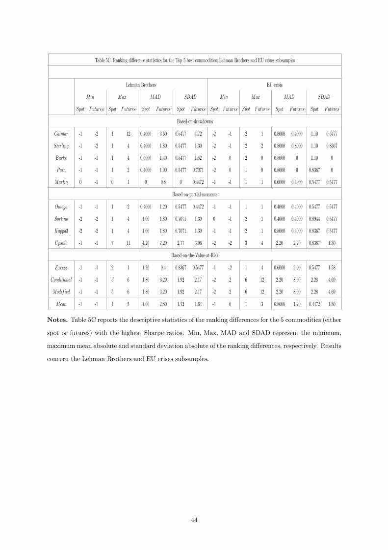
Table 5C. Ranking difference statistics for the Top 5 best commodities; Lehman Brothers and EU crises subsamples

Lehman Brothers EU crisis



Based-on-drawdowns

Calmar -1 -2 1 12 0.4000 3.60 0.5477 4.72 -2 -1 2 1 0.8000 0.4000 1.10 0.5477

Sterling -1 -2 1 4 0.4000 1.80 0.5477 1.30 -2 -1 2 2 0.8000 0.8000 1.10 0.8367

Burke -1 -1 1 4 0.6000 1.40 0.5477 1.52 -2 0 2 0 0.8000 0 1.10 0

Pain -1 -1 1 2 0.4000 1.00 0.5477 0.7071 -2 0 1 0 0.8000 0 0.8367 0

Martin 0 -1 0 1 0 0.8 0 0.4472 -1 -1 1 1 0.6000 0.4000 0.5477 0.5477


Omega -1 -1 1 2 0.4000 1.20 0.5477 0.4472 -1 -1 1 1 0.4000 0.4000 0.5477 0.5477

Sortino -2 -2 1 4 1.00 1.80 0.7071 1.30 0 -1 2 1 0.4000 0.4000 0.8944 0.5477

Kappa3 -2 -2 1 4 1.00 1.80 0.7071 1.30 -1 -1 2 1 0.8000 0.4000 0.8367 0.5477

Upside -1 -1 7 11 4.20 7.20 2.77 3.96 -2 -2 3 4 2.20 2.20 0.8367 1.30


Excess -1 -1 2 1 1.20 0.4 0.8367 0.5477 -1 -2 1 4 0.6000 2.00 0.5477 1.58

Conditional -1 -1 5 6 1.80 3.20 1.92 2.17 -2 2 6 12 2.20 8.00 2.28 4.69

Modified -1 -1 5 6 1.80 3.20 1.92 2.17 -2 2 6 12 2.20 8.00 2.28 4.69

Mean -1 -1 4 5 1.60 2.80 1.52 1.64 -1 0 1 3 0.8000 1.20 0.4472 1.30

Notes. Table 5C reports the descriptive statistics of the ranking differences for the 5 commodities (either



concern the Lehman Brothers and EU crises subsamples.

44

Table 5D. Ranking difference statistics for the Top 5 best commodities; Greek and Post-debt crises subsamples

Greek crisis Post-debt crisis



Based-on-drawdowns

Calmar -2 -2 2 5 1.40 2.40 0.5477 1.82 -2 -1 4 5 2.40 1.80 1.52 1.92

Sterling -4 -4 2 2 2.00 2.00 1.22 1.22 -2 0 2 2 1.20 0.8000 0.8367 1.10

Burke -1 -1 1 1 0.4000 0.8000 0.5477 0.4472 -1 0 1 2 0.8000 0.4000 0.4472 0.8944

Pain -1 -4 1 2 0.8000 1.60 0.4472 1.52 -2 0 2 2 0.8000 0.6000 1.10 0.8944

Martin -1 0 1 0 0.4000 0 0.5477 0 -1 -1 1 1 0.6000 0.6000 0.5477 0.5477


Omega -2 -4 1 1 0.8000 1.60 0.8367 1.34 -1 0 2 1 0.8000 0.4000 0.8367 0.5477

Sortino -1 0 1 0 0.4000 0 0.5477 0 -2 -1 2 1 0.8000 0.8000 1.10 0.4472

Kappa3 -1 0 1 1 0.4000 0.2000 0.5477 0.4472 -2 -1 2 2 0.8000 1.00 1.10 0.7071

Upside -3 1 6 11 3.20 8.60 1.64 4.34 -2 2 7 14 5.00 7.80 2.35 5.02


Excess -2 -1 2 1 1.20 0.4000 0.8367 0.5477 -2 -1 1 7 1.00 2.00 0.7071 2.92

Conditional -2 0 7 13 3.20 2.80 2.28 5.72 -2 -2 2 14 1.60 6.00 0.5477 6.48

Modified -2 0 7 13 3.20 2.80 2.28 5.72 -2 -2 2 14 1.60 6.00 0.5477 6.48

Mean -2 0 4 6 2.60 1.20 1.14 2.68 -2 -1 2 6 1.40 2.60 0.5477 2.70

Notes. Table 5D reports the descriptive statistics of the ranking differences for the 5 commodities (either



concern the Greek and Post-debt crises subsamples.

45

performance evaluation of commodity investments

Documents