performance evaluation in all-wireless wi-fi networks
TRANSCRIPT

UNIVERSIDADE TÉCNICA DE LISBOA
INSTITUTO SUPERIOR TÉCNICO
Performance Evaluation in
All-Wireless Wi-Fi Networks
Gonçalo Caldeira Carpinteiro
(Licenciado)
Dissertation submitted for obtaining the degree of
Master in Electrical and Computer Engineering
Supervisor: Doutor Luís Manuel de Jesus Sousa Correia
Jury
President: Doutor Luís Manuel de Jesus Sousa Correia
Members: Doutor Rui Manuel Rodrigues Rocha
Doutor Rui Luís Andrade Aguiar
April 2008


i
Acknowledgements
Acknowledgements
Firstly, I would like to thank Prof. Luís Correia for having supervised this work. He always
provided me the knowledge and motivation to achieve the proposed objectives and to distinguish
what is important from what is not.
To Lúcio Ferreira and Martijn Kuipers, I would like to thank the profitable discussions on WIP
project details, which were very useful on setting down the main goals of this work. To Daniel
Sebastião, who joined me on the task of tackling OPNET Modeler nuts and bolts. To all of them
and to Carla Oliveira, with whom I shared a positive and vibrant working environment at the
beginning of this work.
A special thanks to Inês, who teaches me how to “always look on the bright side of life”.
Somehow, this is her work too.
At last but not least, I would like to thank all my Family and Friends, for their constant support
and encouragement.

iii
Abstract
Abstract
This study aims at establishing a set of basic requirements for the network architecture of an
all-wireless Internet, implemented using mesh network concepts exclusively with WLANs. These
requirements can be used as inputs to more in-depth investigations, such as the WIP project. An
Implementation Model to evaluate network performance at single hop level is defined, with the
objective to assess the impact of the variation of several network parameters. A detailed analysis
of the results obtained from several simulation runs with OPNET Modeler reveals that: the
standard for backbone network with better performance is 802.11a; the number of clients
associated to each mesh access point must be lower than 30; the distance between mesh Access
Points must be lower than 140 m; the minimum nominal data rate at the backbone is 5.5 Mbps;
and mesh Access Points buffer size must be greater than 64 kbits. Using these requirements, the
maximum throughput obtained at the backbone network is 5.35 Mbps, the FTP response time is
10 s, and the VoIP end-to-end delay is 60 ms. These values can be used as figures of merit of the
network in order to measure the relative gain of future network architecture and protocol
enhancements.
Keywords
Wireless Mesh Network. All-Wireless Internet. WLANs. Service Mix. Mesh Access Points.

iv
Resumo
Resumo Este trabalho pretende estabelecer um conjunto de requisitos básicos para a arquitectura de uma
all-wireless Internet, implementada usando os conceitos de redes mesh exclusivamente com
WLANs. Estes requisitos podem ser utilizados como pontos de partida para investigações mais
detalhadas, tais como o projecto WIP. Foi desenvolvido um Modelo de Implementação para a
análise da performance da ligação entre dois pontos de acesso mesh, com o objectivo de avaliar o
impacto da variação de vários parâmetros da rede. A análise detalhada dos resultados de várias
simulações usando a ferramenta OPNET Modeler revela que: a norma com melhor performance
para a rede backbone é a 802.11a; o número de clientes associados a cada um dos pontos de acesso
mesh deve ser menor que 30; a distância entre pontos de acesso mesh deve ser menor que 140 m; o
ritmo de transmissão nominal mínimo, na rede backbone, deve ser 5.5 Mbps; e o tamanho da
memória dos pontos de acesso mesh deve ser superior a 64 kbits. Tendo em conta estes requisitos,
obteve-se um ritmo de transmissão máximo na rede backbone de 5.35 Mbps, um tempo de
resposta para a aplicação FTP de 10 s, e um atraso ponto-a-ponto para a aplicação VoIP de 60
ms. Estes valores podem ser considerados como figuras de mérito, com o objectivo de medir o
ganho relativo de melhorias futuras da arquitectura da rede e dos vários protocolos usados.
Palavras-chave
Rede Mesh Sem Fios. All-Wireless Internet. WLANs. Mistura de Serviços. Pontos de Acesso Mesh.

v
Table of Contents
Table of Contents
Acknowledgements ........................................................................................... i
Abstract ............................................................................................................ iii
Resumo ............................................................................................................ iv
Table of Contents ............................................................................................. v
List of Figures ................................................................................................. vii
List of Tables ................................................................................................... xi
List of Abbreviations ..................................................................................... xiii
List of Symbols .............................................................................................. xvi
List of Programs ........................................................................................... xvii
1 Introduction ...........................................................................................1
1.1 Overview ........................................................................................................ 2
1.2 Motivation and Contents .............................................................................. 6
2 802.11 Wireless LANs ............................................................................ 9
2.1 802.11 WLANs Overview .......................................................................... 10
2.2 802.11 Medium Access Control ................................................................ 14
2.2.1 MAC Data Services ................................................................................................ 14
2.2.2 MAC Frame Formats ............................................................................................. 19
2.3 802.11 Physical Layer .................................................................................. 22
2.3.1 The Various Physical Layers ................................................................................. 22
2.3.2 802.11a WLANs ...................................................................................................... 23
2.3.3 802.11b WLANs ..................................................................................................... 25
2.3.4 802.11g WLANs...................................................................................................... 26

vi
2.4 WLANs Backbone ...................................................................................... 27
2.5 Services and Applications ........................................................................... 32
3 Simulations of WLANs with Wireless Backbone .............................. 37
3.1 WLANs with Wireless Backbone .............................................................. 38
3.1.1 Related Work ........................................................................................................... 38
3.1.2 Performance Analysis of a Wireless Backbone .................................................. 43
3.2 OPNET Modeler Basics ............................................................................. 46
3.2.1 Initial Considerations ............................................................................................. 46
3.2.2 Modelling Domains ................................................................................................ 47
3.2.3 Discrete Event Simulations ................................................................................... 52
3.2.4 Data Collection and Analysis ................................................................................ 54
3.2.5 WLAN Models ........................................................................................................ 57
3.3 WLANs with Wireless Backbone using OPNET ................................... 60
4 Results Analysis .................................................................................. 65
4.1 Simulations Setup ........................................................................................ 66
4.2 Service Mix ................................................................................................... 74
4.3 Distance – MAPs ......................................................................................... 85
4.4 Number of Clients ....................................................................................... 90
4.5 Data Rate ...................................................................................................... 94
4.6 Buffer Size .................................................................................................... 99
4.7 Wired vs. Wireless Backbone ................................................................... 102
5 Conclusions ........................................................................................ 103
Annex A Applications Attributes ................................................................ 109
Annex B Results of Applications Evaluation Metrics ............................... 113
References ...................................................................................................... 123
vii
List of Figures
List of Figures Figure 1.1. Wireless Mesh Network (based on IEEE 802.11 standards). ............................................ 4
Figure 1.2. WIP project – The Radio Internet (extracted from [Fdid07]). .......................................... 5
Figure 1.3. Scope of the study. ................................................................................................................... 7
Figure 2.1. OSI and IEEE 802.11 reference models (adapted from [Stal05]). ................................. 10
Figure 2.2. Extended service set. .............................................................................................................. 12
Figure 2.3. CW value after several successive retransmission attempts. ............................................ 16
Figure 2.4. Timeline of DCF operation (adapted from [IEEE99]). ................................................... 16
Figure 2.5. Use of RTS/CTS frames (extracted from [IEEE99]). ...................................................... 17
Figure 2.6. DCF medium access process. ............................................................................................... 18
Figure 2.7. CF repetition interval. ............................................................................................................ 19
Figure 2.8. The general IEEE 802.11 MAC frame. .............................................................................. 19
Figure 2.9. IEEE 802.11a PPDU. ............................................................................................................ 24
Figure 2.10. IEEE 802.11b PPDU short format. .................................................................................. 25
Figure 2.11. IEEE 802.3 topologies. ....................................................................................................... 28
Figure 2.12. Data exchange definition (adapted from [OPMo06]). .................................................... 33
Figure 3.1. Basic approaches to wireless mesh networks. .................................................................... 39
Figure 3.2. Implementation model. ......................................................................................................... 45
Figure 3.3. Project editor (network domain) with an example of a network model. ....................... 48
Figure 3.4. Some node models representations. .................................................................................... 49
Figure 3.5. Example of a node model description. ............................................................................... 49
Figure 3.6. Examples of modules available at node domain. ............................................................... 50
Figure 3.7. Connections between modules in the node domain. ........................................................ 50
Figure 3.8. Developing a process model with processor editor. ......................................................... 51
Figure 3.9. Typical simulation timeline. .................................................................................................. 53
Figure 3.10. Aspect of a Choose Results window (accessible from project editor). ........................ 55
Figure 3.11. Example of a vector data analysis panel............................................................................ 56
Figure 3.12. Example of a scalar data analysis panel. ............................................................................ 56
Figure 3.13. Internal structure of wlan_wkstn node model. .................................................................. 58
Figure 3.14. Internal structure of wlan_station node model. ................................................................. 58

viii
Figure 3.15. Internal structure of wlan2_router node model. ................................................................. 59
Figure 3.16. WLAN Node and Module statistics. ................................................................................. 59
Figure 3.17. Implementation model using OPNET Modeler. ............................................................ 60
Figure 3.18. Static Routing Table attribute. ............................................................................................ 62
Figure 4.1. Representation of Profile_1 and Profile_4 attributes (adapted from [OPMo06]). ....... 68
Figure 4.2. Δ for two sets of 25 Seeds (with X = R in BSS2). ............................................................ 73
Figure 4.3. Global Delay for 25 simulation runs. .................................................................................. 73
Figure 4.4. Rcum_10 in MAP1 vs. AD. ......................................................................................................... 75
Figure 4.5. Rcum_10 in MAP2 vs. AD. ......................................................................................................... 75
Figure 4.6. _10cum
DLT for MAP1 vs. AD. ..................................................................................................... 77
Figure 4.7. _10cum
DLT for MAP2 vs. AD. ..................................................................................................... 77
Figure 4.8. RMAX_10 in MAP1 vs. AD. ...................................................................................................... 78
Figure 4.9. GR in MAP1 vs. AD. .............................................................................................................. 78
Figure 4.10. Prcvd in MAP1 vs. Technology used in BSS0. ..................................................................... 79
Figure 4.11. 10cum _
TXR for MAP1 vs. AD. .................................................................................................. 81
Figure 4.12. 10cum _
TXR for MAP2 vs. AD. .................................................................................................. 81
Figure 4.13. Qcum_10 in MAP1 vs. AD. ...................................................................................................... 82
Figure 4.14. Qcum_10 in MAP2 vs. AD. ...................................................................................................... 82
Figure 4.15. 10cum _
rtxD for MAP2 vs. AD (at Back11b_SameCh). ........................................................... 83
Figure 4.16. 10cum _
bufD for MAP2 vs. AD (at Back11b_SameCh). ........................................................... 83
Figure 4.17. 10cum _
FTPRT vs. AD. ................................................................................................................... 84
Figure 4.18. 10cum _
VoIPE vs. AD. ..................................................................................................................... 84
Figure 4.19. RMAX_10 in MAP1 vs. D. ....................................................................................................... 85
Figure 4.20. 10cum _
TXR for MAP1 vs. D. ...................................................................................................... 86
Figure 4.21. _10cum
DLT for MAP1 vs. D. ...................................................................................................... 86
Figure 4.22. Qcum_10 in MAP1 vs. D. .......................................................................................................... 87
Figure 4.23. 10cum _
FTPRT vs. D. ...................................................................................................................... 87
Figure 4.24. 10cum _
VoIPE vs. D.......................................................................................................................... 88
Figure 4.25. RMAX_10 in MAP1 vs. distance between MAPs (receivers’ sensitivity set to -76 dBm). ................................................................................................................................. 89
Figure 4.26. RMAX_10 in MAP1 vs. N. ....................................................................................................... 90
Figure 4.27. GR in MAP1 vs. N. ............................................................................................................... 91
Figure 4.28. 10cum _
TXR for MAP1 vs. N. ..................................................................................................... 92

ix
Figure 4.29. _10cum
DLT for MAP1 vs. N. ..................................................................................................... 92
Figure 4.30. Qcum_10 in MAP1 vs. N........................................................................................................... 93
Figure 4.31. 10cum _
FTPRT vs. N. ...................................................................................................................... 93
Figure 4.32. 10cum _
VoIPE vs. N. ........................................................................................................................ 94
Figure 4.33. RMAX_10 in MAP1 vs. RN in BSS0. ....................................................................................... 95
Figure 4.34. 10cum _
TXR for MAP1 vs. RN in BSS0. ..................................................................................... 96
Figure 4.35. _10cum
DLT for MAP1 vs. RN in BSS0. ..................................................................................... 96
Figure 4.36. Qcum_10 in MAP1 vs. RN in BSS0. ......................................................................................... 97
Figure 4.37. 10cum _
bufD for MAP1 vs. RN in BSS0. ...................................................................................... 97
Figure 4.38. 10cum _
FTPRT vs. RN in BSS0. ..................................................................................................... 98
Figure 4.39. 10cum _
VoIPE vs. RN in BSS0. ........................................................................................................ 98
Figure 4.40. Qcum_10 in MAP1 vs. Bf. ........................................................................................................ 100
Figure 4.41. 10cum _
bufD for MAP1 vs. Bf.. ..................................................................................................... 100
Figure 4.42. 10cum _
FTPRT vs. Bf. .................................................................................................................... 101
Figure 4.43. 10cum _
VoIPE vs. Bf. ....................................................................................................................... 101
Figure 4.44. ADSL2 and ADSL2plus maximum downstream data rates (extracted from [DSLF03]). ...................................................................................................................... 102
Figure B.1. 10cum _
mailDRT vs. AD. .................................................................................................................. 114
Figure B.2. 10cum _
webRT vs. AD. .................................................................................................................. 114
Figure B.3. 10cum _
videoE vs. AD. ..................................................................................................................... 115
Figure B.4. 10cum _
mailDRT vs. D. ..................................................................................................................... 115
Figure B.5. 10cum _
webRT vs. D. ..................................................................................................................... 116
Figure B.6. 10cum _
videoE vs. D. ........................................................................................................................ 116
Figure B.7. 10cum _
mailDRT vs. N. ..................................................................................................................... 117
Figure B.8. 10cum _
webRT vs. N. ..................................................................................................................... 117
Figure B.9. 10cum _
videoE vs. N. ........................................................................................................................ 118
Figure B.10. 10cum _
mailDRT vs. RN in BSS0. ................................................................................................... 118
Figure B.11. 10cum _
webRT vs. RN in BSS0. ................................................................................................... 119
Figure B.12. 10cum _
videoE vs. RN in BSS0. ...................................................................................................... 119

x
Figure B.13. 10cum _
mailDRT vs. Bf. ................................................................................................................... 120
Figure B.14. 10cum _
webRT vs. Bf. ................................................................................................................... 120
Figure B.15. 10cum _
videoE vs. Bf. ...................................................................................................................... 121

xi
List of Tables
List of Tables Table 1.1. Scope of some 802.11 sub-standards. ..................................................................................... 3
Table 2.1. IEEE 802.11 services. ............................................................................................................. 13
Table 2.2. Values for the duration/ID field. .......................................................................................... 21
Table 2.3. Information contained in the different address fields. ....................................................... 21
Table 2.4. IEEE 802.11a data rates. ........................................................................................................ 24
Table 2.5. IEEE 802.11b. .......................................................................................................................... 26
Table 2.6. IEEE 802.11g options. ........................................................................................................... 26
Table 2.7. Estimated distance vs. data rate. ............................................................................................ 27
Table 2.8. IEEE 802.3 10 Mbps PHY layer alternatives. ..................................................................... 30
Table 2.9. IEEE 802.3 100 Mbps PHY layer alternatives. ................................................................... 30
Table 2.10. IEEE 802.3 1 Gbps PHY layer alternatives. ..................................................................... 30
Table 2.11. ADSL technology options (extracted from [DSLF07]). .................................................. 32
Table 2.12. 3GPP Service Classes (adapted from [3GPP06a] and [3GPP06b]). .............................. 33
Table 3.1. Modeler secondary editors – incomplete list (adapted from [OPMo06]). ....................... 52
Table 3.2. Event attributes summary (adapted from [OPMo06]). ...................................................... 54
Table 3.3. Main attributes of wlan_wkstn model instances. ................................................................... 63
Table 3.4. Main attributes of instances of wlan_server model. ............................................................... 64
Table 3.5. Main attributes of instances of wlan2_router model. ............................................................ 64
Table 4.1. Technology used in each BSS. ............................................................................................... 66
Table 4.2. Profiles definition. .................................................................................................................... 67
Table 4.3. Applications Distribution (AD) values. ................................................................................ 68
Table 4.4. Implementation Model – default settings............................................................................. 69
Table 4.5. Service Mix Simulation Set definition. .................................................................................. 69
Table 4.6. Distance – MAPs Simulation Set definition. ....................................................................... 69
Table 4.7. Number of Clients Simulation Set definition. ..................................................................... 70
Table 4.8. Data Rate Simulation Set definition. ..................................................................................... 70
Table 4.9. Buffer Size Simulation Set definition. ................................................................................... 70
Table 4.10. Common Wireless LAN Parameters attributes. ................................................................ 71
Table 4.11. Actual simulation times. ........................................................................................................ 74

xii
Table 4.12. Maximum values of GR. ........................................................................................................ 79
Table 4.13. Calculated maximum distance between MAPs. ................................................................. 88
Table 4.14. Maximum throughput values at backbone network. ........................................................ 91
Table 5.1. Relation between Simulation Sets and degrees of freedom. ............................................ 105
Table 5.2. Maximum throughput values. .............................................................................................. 107
Table 5.3. Basic requirements of a mesh network. .............................................................................. 107
Table A.1. FTP Attributes....................................................................................................................... 110
Table A.2. E-mail attributes. ................................................................................................................... 110
Table A.3. Web Browsing attributes. ..................................................................................................... 111
Table A.4. Web Browsing – Page Properties attribute. ...................................................................... 111
Table A.5. Video Streaming attributes. ................................................................................................. 111
Table A.6. Video Conferencing attributes. ........................................................................................... 112
Table A.7. VoIP attributes. ..................................................................................................................... 112

xiii
List of Abbreviations
List of Abbreviations ACK Acknowledgment.
AD Applications Distribution.
ADSL Asymmetric Digital Subscriber Line.
AID Association Identifier.
AP Access Point.
ATIM Ad-hoc Traffic Indication Message
BSS Basic Service Set.
BSSID BSS Identifier.
CA Collision Avoidance.
CCK Complementary Code Keying.
CD Collision Detection.
CFP Contention-Free Period.
CRC Cyclic Redundancy Check.
CSMA Carrier Sense Multiple Access.
CTS Clear To Send.
CW Contention Window.
DA Destination Address.
DCF Distributed Coordination Function.
DIFS DCF IFS.
DMT Discrete Multitone.
DS Distribution System.
DSSS Direct Sequence Spread Spectrum.
EDCA Enhanced Distributed Access.
ERP Extended Rate Physical.
ESS Extended Service Set.
FCS Frame Check Sequence.
FHSS Frequency Hopping Spread Spectrum.
FTP File Transfer Protocol.
GSM Global System for Mobile Communications.

xiv
HCCA HCF Controlled Channel Access.
HCF Hybrid Coordination Function.
HTTP Hyper Text Transfer Protocol.
IBSS Independent BSS.
IFS Interframe Space.
IP Internet Protocol.
ISM Industrial, Scientific and Medical.
LAN Local Area Network.
LLC Logical Link Control.
MAC Medium Access Control.
MAP Mesh Access Point.
MIMO Multiple Input Multiple Output.
MP Mesh Point.
MPDU MAC Protocol Data Unit.
MSDU MAC Service Data Unit.
NAV Network Allocation Vector.
NIC Network Interface Card.
NoRTiSM Non-Real Time Service Mix.
NRTCeSM Non-Real Time Centric Service Mix.
OFDM Orthogonal Frequency Division Multiplexing.
OSI Open System Interconnection.
PBCC Packet Binary Convolutional Coding.
PDF Probability Density Function.
PC Point Coordinator.
PCF Point Coordination Function.
PHY Physical.
PIFS PCF IFS.
PLC Power Line Communications.
PLCP Physical Layer Convergence Procedure.
PMD Physical Medium Dependent
POP Post Office Protocol.
PPDU PLCP Protocol Data Unit.
PS Power Save.
QoS Quality of Service.
RA Receiver Address.

xv
ReferSM Reference Service Mix.
RF Radiofrequency.
RI Radio Interface.
RTiCeSM Real Time Centric Service Mix.
RTS Request to Send.
SA Source Address.
SFD Start-of-Frame Delimiter.
SIFS Short IFS.
SMTP Simple Mail Transfer Protocol.
STP Shielded Twisted Pair.
TA Transmitter Address.
TCP Transmission Control Protocol.
TDD Time Division Duplex.
TDMA Time Division Multiple Access.
TGs 802.11s Task Group.
UNII Universal Networking Information Infrastructure.
UTP Unshielded Twisted Pair.
VoIP Voicer over IP.
WEP Wired Equivalent Privacy.
WiMAX Worldwide Interoperability for Microwave Access.
WLAN Wireless LAN.

xvi
List of Symbols
List of Symbols
Δ Measure of cumulative mean stability.
Bf Buffer size (in MAP RI2).
D Distance between MAP1 and MAP2.
Dbuf Data dropped due to buffer overflow (in MAP RI2).
Drtx Data dropped due to retransmission threshold exceeded (in MAP RI2).
Evideo Video Streaming and Video Conferencing packet end-to-end delay.
EVoIP VoIP packet end-to-end delay.
GR RMAX_10 gain relative to Back11b_SameCh values.
M Number of servers
N Number of clients.
Prcvd Received packets size (in MAP RI2).
Q Queue size (in MAP RI2).
R Throughput (in MAP RI2).
RN Nominal data rate.
RTX Retransmission attempts (in MAP RI2).
RTFTP FTP download response time.
RTmailD E-mail download response time.
RTmailU E-mail upload response time.
RTweb Web Browsing page response time.
s Simulation run index.
S Total number of simulation runs.
TDL Media access delay (in MAP RI2).
Xcum_s Cumulative mean of a given evaluation metric X at simulation run s.
Xmax_i Maximum value of a given evaluation metric X obtained during simulation run i.
XMAX_s Cumulative maximum value of a given evaluation metric X at simulation run s.
Xmean_i Mean of a given evaluation metric X obtained at a simulation run i.

xvii
List of Programs
List of Programs OPNET Modeler Discrete Event Simulator, implementing all the basic concepts of an objects
programming language. Systems are described in terms of objects, which are instances of models (the OPNET equivalent to classes). There are a vast number of already implemented models addressing several technologies, protocols and commercially available equipment from various suppliers. They provide a user with all the necessary means to develop a complete description of a communication network or an information system.


Introduction
1
Chapter 1
Introduction
1 Introduction
This chapter gives a brief overview of the work, putting it into context and describing its
objectives. The possibility of using the obtained results as the basis for ongoing and future
projects is also emphasised. At the end of the chapter, the work structure is provided.
Performance Evaluation in All-Wireless Wi-Fi Networks
2
1.1 Overview
Today, it is possible to state without any in-depth analysis that IEEE 802.11 Wireless Local Area
Network (WLAN) technology has reached worldwide acceptance for wireless short-range
Internet access. The success of WLANs has led to a massive presence in the market of wireless
networked devices at relatively low prices and to their deployment in several scenarios, mainly as
a last mile solution for broadband wireless access (at homes and isolated hotspots), or as an
extension of wired LANs in small business environments. In fact, these statements are strongly
supported by the following sentence, extracted from a recent WiFi Alliance [WiFi07] press
release:
“WiFi is a pervasive wireless technology used by more than 350 million people at more than
200 000 public hotspots, millions of homes and business worldwide”.
Among many factors, this success was essentially driven by three different aspects: 802.11
WLANs are easy to implement and use; they are built for radio systems in unlicensed spectrum,
which is often harmonised throughout the world; and they are supported by a rapid development
of standards for interoperable products and increasing network performance, demanded by
commercial needs.
The original IEEE 802.11 standard was published in 1997, seven years after the creation of the
802.11 working group. Two years later, in 1999, a revised version [IEEE99] of improved
accuracy was released, together with 802.11a [IEEE99a] and 802.11b [IEEE99b] sub-standards,
as an extension to the original standard physical capacity. Another extension sub-standard,
802.11g [IEEE03], was published in 2003. The scope of these standards is the specification of
the two lowest Open System Interconnection (OSI) reference model layers (1 and 2), defining a
Medium Access Control (MAC) protocol and several physical transmission schemes (802.11a, b
and g).
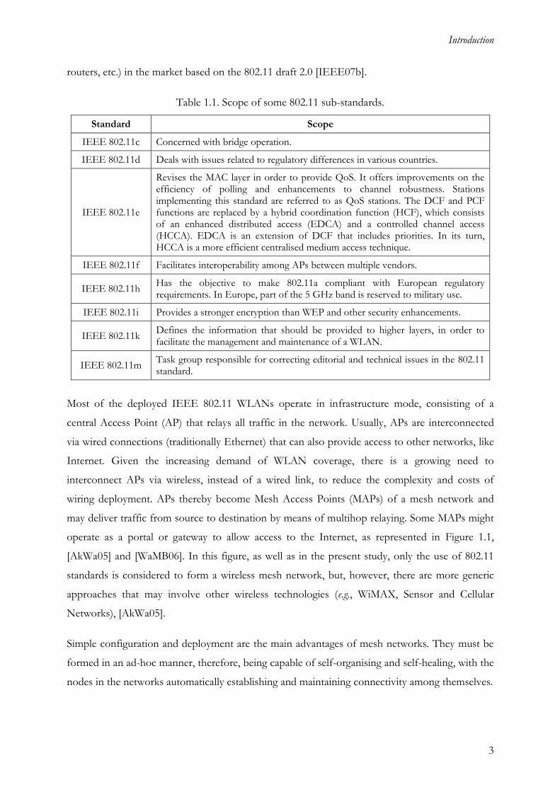
Additionally, 802.11 comprises many more sub-standards, each one addressing particular
extensions, as described in Table 1.1 [Stal04]. Many other sub-standards are currently being
developed, reflecting the 802.11 effort on providing an adequate level of standardisation. A good
example is 802.11n, which specifies a new physical layer scheme aiming at achieving data rates up
to 300 Mbps. It is based on the Multiple Input Multiple Output (MIMO) air interface technology,
which employs multiple receivers and transmitters to transport two or more data streams.
Currently, there are already some WiFi certified products (access points, laptop computers,
Introduction
3
routers, etc.) in the market based on the 802.11 draft 2.0 [IEEE07b].
Table 1.1. Scope of some 802.11 sub-standards.
Standard Scope
IEEE 802.11c Concerned with bridge operation.
IEEE 802.11d Deals with issues related to regulatory differences in various countries.
IEEE 802.11e
Revises the MAC layer in order to provide QoS. It offers improvements on the efficiency of polling and enhancements to channel robustness. Stations implementing this standard are referred to as QoS stations. The DCF and PCF functions are replaced by a hybrid coordination function (HCF), which consists of an enhanced distributed access (EDCA) and a controlled channel access (HCCA). EDCA is an extension of DCF that includes priorities. In its turn, HCCA is a more efficient centralised medium access technique.
IEEE 802.11f Facilitates interoperability among APs between multiple vendors.
IEEE 802.11h Has the objective to make 802.11a compliant with European regulatory requirements. In Europe, part of the 5 GHz band is reserved to military use.
IEEE 802.11i Provides a stronger encryption than WEP and other security enhancements.
IEEE 802.11k Defines the information that should be provided to higher layers, in order to facilitate the management and maintenance of a WLAN.
IEEE 802.11m Task group responsible for correcting editorial and technical issues in the 802.11 standard.
Most of the deployed IEEE 802.11 WLANs operate in infrastructure mode, consisting of a
central Access Point (AP) that relays all traffic in the network. Usually, APs are interconnected
via wired connections (traditionally Ethernet) that can also provide access to other networks, like
Internet. Given the increasing demand of WLAN coverage, there is a growing need to
interconnect APs via wireless, instead of a wired link, to reduce the complexity and costs of
wiring deployment. APs thereby become Mesh Access Points (MAPs) of a mesh network and
may deliver traffic from source to destination by means of multihop relaying. Some MAPs might
operate as a portal or gateway to allow access to the Internet, as represented in Figure 1.1,
[AkWa05] and [WaMB06]. In this figure, as well as in the present study, only the use of 802.11
standards is considered to form a wireless mesh network, but, however, there are more generic
approaches that may involve other wireless technologies (e.g., WiMAX, Sensor and Cellular
Networks), [AkWa05].
Simple configuration and deployment are the main advantages of mesh networks. They must be
formed in an ad-hoc manner, therefore, being capable of self-organising and self-healing, with the
nodes in the networks automatically establishing and maintaining connectivity among themselves.

Performance Evaluation in All-Wireless Wi-Fi Networks
4
Internet
802.11a
Network802.11b
Network
802.11b
Network
MAP1
with Gateway
MAP5MAP4
MAP6
MAP3
STAT1
STAT5STAT3STAT2
STAT4
STAT6
MAP2
with Gateway
Wired link
Wireless link
Backbone
Figure 1.1. Wireless Mesh Network (based on IEEE 802.11 standards).
Given their unique characteristics, mesh networks have a wide range of potential applications,
such as, [AkWa05]:
Broadband home networking – The deployment of MAPs in a home environment can easily
reduce zones without service coverage. Network capacity is also better compared with the
traditional solution of having APs connected to an access modem or hub via wire.
Community and neighbourhood networking – Mesh networks can simplify the connectivity of
users inside a community allowing direct links (or indirect via multiple hops) among them.
Applications such as distributed file access and video streaming are then facilitated.
Enterprise networking – The traditional application of WLAN networks in such scenarios is
the use of APs providing isolated “islands” of wireless access, connected to the wired
enterprise networks. The replacement of this topology by a mesh network presents several
advantages, e.g., the elimination of most Ethernet wires and the improvement of network
resource usage.
Metropolitan area networks – Considerations on this scenario are similar to the previous ones
related to enterprise networking, taking into account that a much larger area is covered, and
that scalability requirements assume an important role during network configuration.
Transportation systems – Mesh networks support convenient passenger information services,
remote monitoring of in-vehicle security video, and driver communications.
Building automation – Equipments, like elevators, air conditioners, electrical power devices,
etc., need to be controlled/monitored, thus, connected among themselves and to some sort of
central controller. This task can be greatly improved, and deployment costs greatly reduced if

Introduction
5
mesh networks are used.
Health and medical systems – For several purposes, there is the need to transmit broadband
data from one room to another. Transmission of high resolution medical images and various
periodical monitoring signals can generate a large volume of data, which can be handled by a
mesh network.
Security surveillance systems – Similar to the two previous applications, mesh networks are
adequate to connect several security surveillance systems in buildings, shopping malls, stores,
etc..
Due to all these possible usage scenarios, mesh networks are being extensively studied since the
past few years. Many works can be found in literature addressing several open issues that still
need to be answered. Along this effort, is the work of 802.11s task group (TGs) [IEEE07a],
which aim is to standardise a mesh WLAN as a network of interconnected APs. Stations served
by the several APs are interconnected through multihop operations, and may be also connected
to other broadcast domains via a portal or a gateway.
Taking the concept of mesh networking a step further, the WIP Project [WIPw07], under the
European IST Work Programme in FP6, aims at building an all-wireless network that can grow
and gradually replace the existing wired Internet. This new wireless communication
infrastructure, also called Radio Internet, will be based on the cooperation among APs of
unlicensed spectrum networks, forming a backbone that will require only limited access to the
wired infrastructure. Then, wireless networks are not only the access technology but also the core
of the network. Figure 1.2 represents the vision of the Radio Internet.
Figure 1.2. WIP project – The Radio Internet (extracted from [Fdid07]).

Performance Evaluation in All-Wireless Wi-Fi Networks
6
Such ambitious objectives require investigation on several issues, such as: wireless transmission
techniques, mesh networking, cross-layer optimisation, mechanisms for seamless mobility, and
self-organisation.
At the moment of the writing of this thesis, the WIP Project is at its intermediate stages, with the
Final Report planned for submission at January 2009.
1.2 Motivation and Contents
More than a promising technology, mesh networking is now considered a fundamental
instrument to enable a ubiquitous wireless Internet. The combination of wireless forwarding and
routing protocols allows the establishment of all wireless end-to-end routes among
communicating devices placed far away from each other, which could not exist if only standard
802.11 networks were used.
As mentioned in the previous section, the increasing importance of mesh networks and the great
number of foreseen applications has driven them to become a hot topic in wireless
communications research worldwide. Nevertheless, there is still a number of challenging research
topics at all protocol layers level that need to be addressed, in order to take advantage of all mesh
network potentialities. Among them is the identification of the relationship between network
capacity and other factors, such as: network architecture, network topology, traffic pattern,
network node density, number of channels used for each node, transmission power level and
node mobility, [AkWa05]. A good understanding of this relationship provides a guideline for
protocol development, architecture design, deployment and operation of the network.
The study of a network capacity is usually performed considering the network as a whole,
obtaining generic conclusions that sometimes can neglect the influence of some details, only
measured by a more fine-tuned analysis. Taking this observation into account, the present study
aims at evaluating the impact of several parameters into mesh networks capacity and
performance, not at a global perspective but instead at a single hop level, Figure 1.3.
This investigation is motivated by the need of establishing basic requirements and starting points
for other major studies (the WIP project, for instance) dedicated to design more complex
networks based on a mesh technology.

Introduction
7
Internet
802.11a
Network802.11b
Network
802.11b
Network
MAP1
with Gateway
MAP5MAP4
MAP6
MAP3
STAT1
STAT5STAT3STAT2
STAT4
STAT6
MAP2
with Gateway
Wired link
Wireless link
Backbone
Single hop link within
the mesh network.
Figure 1.3. Scope of the study.
Specifically, the impact of the following parameters is considered:
802.11 standard used within the backbone network – To investigate which of the existing
standards (802.11a, b or g) has a better performance when used at the backbone network.
The traffic mix delivered to the network – To establish network capacity in several scenarios
of traffic load.
Distance between MAPs – To obtain a minimum MAP density.
Number of stations associated to each MAP – To obtain a maximum of stations that can be
associated to each MAP.
Nominal data rate in backbone network – To evaluate which data rates do not satisfy
backbone requirements.
Internal buffer size of MAPs forming the network – To investigate if buffer size is a limitative
factor in network performance.
The obtained results allow the establishment of a reference single hop performance, together
with basic requirements for mesh network deployment, using 802.11 standards on both access
and backbone networks.
To address these issues in a convenient manner, the present document is composed of 5
chapters, including the present one, and two annexes. The following chapter presents all the
aspects of IEEE 802.11 standards that are relevant to the study. Moreover, two other issues that
are not directly related to 802.11 set of standards are also presented, which are an overview of the
most common technologies used as WLANs backbone, and a brief description of the services

Performance Evaluation in All-Wireless Wi-Fi Networks
8
and applications that can be found on this type of networks. Subsequently, Chapter 3 describes
the basic aspects of wireless backbones implemented with 802.11, reviewing several works found
in the literature. The remaining of the chapter is dedicated to the description of the used
simulation tool, OPNET Modeler, and to the detailed presentation of the simulation model and
its implementation. In Chapter 4, the results obtained from several simulation sets are presented,
pointing out the most important observations. Finally, Chapter 5 finalises the thesis, drawing
conclusions and providing some considerations about future work. Annex A describes and
provides values for the attributes of applications forming the traffic mix, while Annex B presents
all applications related simulation results.

802.11 Wireless LANs
9
Chapter 2
802.11 Wireless LANs
2 802.11 Wireless LANs
This chapter provides an overview of IEEE 802.11 WLANs, mainly focussing on the Medium
Access Control (MAC) Layer. A brief description of the Physical Layer (PHY) is also presented
as well as the most common alternatives for the WLAN backbone.

Performance Evaluation in All-Wireless Wi-Fi Networks
10
2.1 802.11 WLANs Overview
Resembling wired LANs, WLANs are organised in terms of a layering of protocols that
cooperate to provide all the basic functions of a LAN. All layers have their own functions that
rely on the ones provided by the layers immediately below. This section opens with a description
of the protocol architecture for WLANs, and then an overview is given on existing topologies
and services provided by WLANs, in order to have a global perspective of the system, [IEEE99]
and [RoLe05].
Regarding the OSI reference model, depicted in Figure 2.1, one can say that higher layer
protocols (network layer and above) are independent of the network architecture. This way, a
description of WLANs protocols is concerned mainly with lower layers of the OSI model. Figure
2.1 shows the correspondence between the WLANs protocols and the OSI architecture,
identifying the scope of IEEE 802.11 standards.
Medium
Physical
Data link
Network
Transport
Session
Presentation
Application
Medium
Physical medium
dependent
Physical layer
convergence procedure
Medium access control
Logical link control
Upper- layer
protocols
Scope of
IEEE
802.11
Figure 2.1. OSI and IEEE 802.11 reference models (adapted from [Stal05]).
Starting from the bottom, the PHY layer provides the following functions:
encoding/decoding of signals;
802.11 Wireless LANs
11
preamble generation/removal;
bit transmission/reception;
specification of the transmission medium and the topology.
As shown in Figure 2.1, for the 802.11 standard, the PHY layer is further divided into two
sublayers, the Physical Layer Convergence Procedure (PLCP) and the Physical Medium
Dependent Sublayer (PMD).
The PLCP is essentially a handshaking layer between MAC and PMD. It defines a method of
mapping MAC Protocol Data Units (MPDUs) onto an appropriate frame format to be
transmitted over the PMD, which defines the method of transmitting and receiving user data
through a wireless medium.
The functions associated with the MAC layer are above the PHY one. These include:
frame addressing (on transmission) and address recognition (on reception);
error detection;
control of the access to transmission medium.
All these functions are detailed in the next sections.
The concept of service set is the basis of the different types of WLAN topologies. A service set is
a grouping of devices that access the network by broadcasting a signal across a wireless radio
frequency (RF) carrier. Having this concept in mind, it is possible to identify the following
topologies:
Basic Service Set (BSS);
Independent Basic Service Set (IBSS);
Extended service set (ESS).
In a BSS, the service set consists of two entities: the station and the AP. There can be several
stations that communicate with one another via the AP, which acts as a relay station. An AP can
also function as a bridge to the outside world, providing a connection to some kind of backbone
Distribution System (DS).
The role of an AP does not exist in an IBSS. Stations communicate directly with one another
without the use of an intermediate. This self-contained network is a simple peer-to-peer WLAN,
which is also referred to as an ad-hoc network. Typically, an IBSS is small and only lasts enough
time until the communication being performed is completed.

Performance Evaluation in All-Wireless Wi-Fi Networks
12
The ESS is the most generic topology for a WLAN, consisting of two or more BSSs that are
interconnected by a DS. Figure 2.2 shows a simple representation of an ESS, where it is possible
to identify a collection of BSSs, grouped via a DS. In this case, if STAT6, located in BSS2, wants
to send a frame to STAT3, it has to send it first to STAT5, which acts as the AP of BSS2, being
responsible for forwarding the frame to STAT1 (the AP of BSS1). Finally, STAT1 is able to
deliver the frame to its final destination. It is important to note that this process is performed at
the MAC level, thus, the ESS appears as a single logical unit to the Logic Link Control (LLC)
one. This way, the frame that is exchanged according to the described process between MAC
users is known as the MAC Service Data Unit (MSDU). Moreover, the MSDU delivery from the
MAC to the upper layer constitutes the basic service of a WLAN.
AP
STAT1
STAT5
AP
Distribution
System
STAT2
STAT3
STAT4
STAT6
STAT7
STAT8
BSS1
BSS2ESS
Figure 2.2. Extended service set.
From the above simple description of a frame traversing an ESS, the need of the IEEE 802.11
standard to define a set of complementary services for the basic MSDU delivery becomes
evident, which are listed in Table 2.1. The provider column indicates who is responsible for the
service. Station services are provided among all stations, therefore, being implemented in every
802.11 station, including APs. Distribution services are available among BSSs, by the DS, being
implemented only in APs or in another special-purpose device attached to the DS.
802.11 Wireless LANs
13
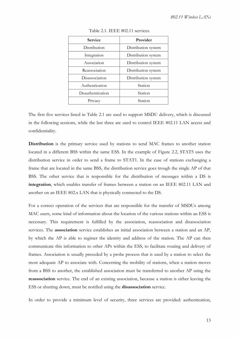
Table 2.1. IEEE 802.11 services.
Service Provider
Distribution Distribution system
Integration Distribution system
Association Distribution system
Reassociation Distribution system
Disassociation Distribution system
Authentication Station
Deauthentication Station
Privacy Station
The first five services listed in Table 2.1 are used to support MSDU delivery, which is discussed
in the following sessions, while the last three are used to control IEEE 802.11 LAN access and
confidentiality.
Distribution is the primary service used by stations to send MAC frames to another station
located in a different BSS within the same ESS. In the example of Figure 2.2, STAT5 uses the
distribution service in order to send a frame to STAT1. In the case of stations exchanging a
frame that are located in the same BSS, the distribution service goes trough the single AP of that
BSS. The other service that is responsible for the distribution of messages within a DS is
integration, which enables transfer of frames between a station on an IEEE 802.11 LAN and
another on an IEEE 802.x LAN that is physically connected to the DS.
For a correct operation of the services that are responsible for the transfer of MSDUs among
MAC users, some kind of information about the location of the various stations within an ESS is
necessary. This requirement is fulfilled by the association, reassociation and disassociation
services. The association service establishes an initial association between a station and an AP,
by which the AP is able to register the identity and address of the station. The AP can then
communicate this information to other APs within the ESS, to facilitate routing and delivery of
frames. Association is usually preceded by a probe process that is used by a station to select the
most adequate AP to associate with. Concerning the mobility of stations, when a station moves
from a BSS to another, the established association must be transferred to another AP using the
reassociation service. The end of an existing association, because a station is either leaving the
ESS or shutting down, must be notified using the disassociation service.
In order to provide a minimum level of security, three services are provided: authentication,
Performance Evaluation in All-Wireless Wi-Fi Networks
14
deauthentication and privacy. Before the association process is accomplished, the station that
wants to communicate with another one needs to prove its identity using the authentication
service. The standard does not mandate any particular authentication scheme, which can range
from a simple handshaking to a public key encryption scheme. The reverse process, when an
existing authentication is to be terminated, is performed by the deauthentication service.
Another security mechanism, used to prevent messages from being read by a casual
eavesdropper, is the privacy service. This service consists of an optional encryption mechanism
that takes the content of a data frame and passes it through an encryption algorithm, in both the
sending and the receiving stations.
Security in a WLAN is a complex issue that is not the object of this thesis. A more detailed
discussion of access and confidentiality services can be found in [RoLe05].
2.2 802.11 Medium Access Control
While the previous section presents a general overview of the IEEE 802.11 standard, describing
the services it provides to other layers in the protocol stack, this section looks into more detail to
the MAC layer and to the functionalities it provides. Section 2.2.1 describes the MAC data
services that are responsible for carrying out data frame exchanges among WLAN stations, and
Section 2.2.2 looks at the general frame format that support MAC layers protocol operation.
Besides data services, the MAC layer also provides management services that range from simple
session management and power control to synchronisation. They are fundamental for a correct
network operation, but are out of the scope of the present study. For a detailed description on
MAC management services refer to [IEEE99] or [RoLe05].
2.2.1 MAC Data Services
MAC data services are responsible for carrying out MSDUs exchange among peer LLC entities,
while the local MAC uses the underlying PHY layer services to transport an MSDU to a peer
MAC entity. This frame exchange between MAC entities requires a mechanism to access the
common medium in a WLAN.

802.11 Wireless LANs
15
The basic medium access protocol used by the MAC layer is a distributed control mechanism,
where each station has equal opportunity to access the medium. This technique, named
Distributed Coordination Function (DCF), is based on a Carrier Sense Multiple Access (CSMA)
with Collision Avoidance (CA) protocol that provides an asynchronous data service.
In the CSMA/CA protocol, a station intending to send data senses the medium first. If the
medium is found idle, the station is able to transmit. Otherwise, if the medium is busy, the station
does not transmit, in order to avoid a collision, picking instead a random backoff time, after
which it tries to access the medium again.
The first step in the DCF is the carrier sense mechanism, in order to assess the state of the
medium. A station trying to determine if the medium is idle has to go through two methods:
check the PHY layer to see whether a carrier is present;
use the virtual carrier sense function, the Network Allocation Vector (NAV).
Just checking the PHY layer is not enough, because although the medium may seem idle, it might
still be reserved by other station via the NAV. Basically, the NAV is a timer that is present in
every station, being updated by data frames transmitted on the medium. Every transmitted frame
has a duration field that is used by other stations to update their NAVs. This process is only
possible because the wireless medium is a broadcast-based shared one.
All stations contending the medium, the ones that transmit successfully and the ones that defer
transmission because the medium is found busy, have to pass through a backoff procedure,
which ensures a low probability of collision, and fair access opportunities for every station. Each
station has a backoff clock that is initiated with a random number of slot times selected from 0 to
the Contention Window (CW) value that the station must wait before it may transmit. The slot
time duration is derived from the PHY, based on the RF characteristics of the BSS. The CW
value varies from a starting CWmin to a maximum CWmax. Each successive attempt to transmit
the same packet is preceded by backoff within a window that doubles the size of the previous
one, as shown in the example illustrated in Figure 2.3.
In the receiving station, the received data frame must be acknowledged to the transmitting one.
This exchange is treated as a unit that cannot be interrupted by a transmission from another
station. If, by any reason, the transmitting station does not receive an Acknowledgment (ACK)
within a specific period of time, it tries to retransmit the frame. This scheme, together with the
use of Request To Send (RTS)/Clear to Send (CTS) frames, discussed later in this section,
Performance Evaluation in All-Wireless Wi-Fi Networks
16
provide the MAC layer with reliable data delivery mechanisms that are able to deal with errors. A
station trying to transmit an ACK frame does not need to pass through the usual backoff
procedure, and after receiving a data frame it can immediately access the medium. This way, the
need for having different interframe spacings in order to provide multiple priorities for medium
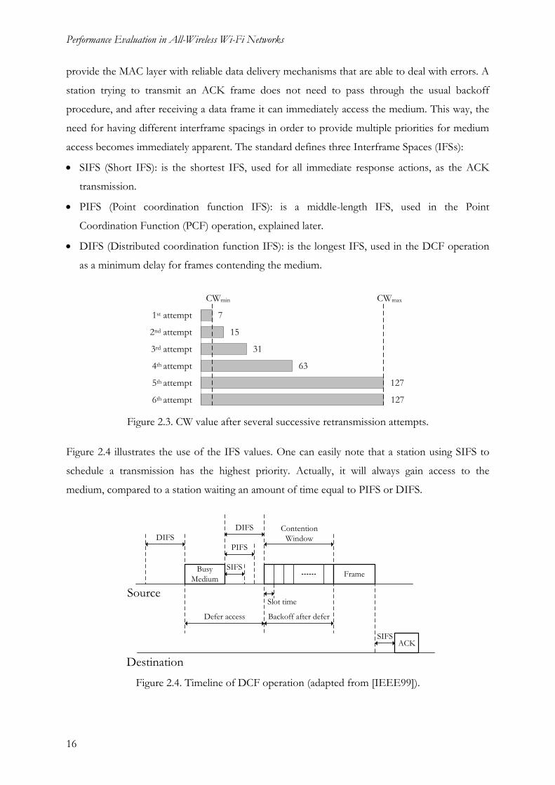
access becomes immediately apparent. The standard defines three Interframe Spaces (IFSs):
SIFS (Short IFS): is the shortest IFS, used for all immediate response actions, as the ACK
transmission.
PIFS (Point coordination function IFS): is a middle-length IFS, used in the Point
Coordination Function (PCF) operation, explained later.
DIFS (Distributed coordination function IFS): is the longest IFS, used in the DCF operation
as a minimum delay for frames contending the medium.
7
15
31
63
127
127
CWmin CWmax
1st attempt
2nd attempt
3rd attempt
4th attempt
5th attempt
6th attempt
Figure 2.3. CW value after several successive retransmission attempts.
Figure 2.4 illustrates the use of the IFS values. One can easily note that a station using SIFS to
schedule a transmission has the highest priority. Actually, it will always gain access to the
medium, compared to a station waiting an amount of time equal to PIFS or DIFS.
Busy
MediumFrame
Contention
WindowDIFS
DIFS
PIFS
SIFS
Slot timeSource
Defer access Backoff after defer
ACK
Destination
SIFS
Figure 2.4. Timeline of DCF operation (adapted from [IEEE99]).

802.11 Wireless LANs
17
As already mentioned, the use of RTS/CTS messages is another mechanism that provides reliable
data delivery. A station attempts to reserve the medium by sending a RTS frame that must go
through the DCF process as any normal frame would. This frame indicates the expected duration
of the future frame exchange to all stations within its range. The destination of the RTS frame
replies with a CTS frame after waiting a SIFS. All other stations receiving the CTS frame update
their NAVs to the time needed for the entire frame (including ACK) to be transmitted. When
large MPDUs are to be transmitted, RTS/CTS handshaking can improve the MAC efficiency,
even in the presence of hidden terminals, i.e., pairs of terminals that may not directly hear one
another. In fact, when a collision occurs, the time wasted while the medium is busy is smaller
when a RTS/CTS exchange is used than when the MPDU is transmitted immediately following
the DIFS. The use of RTS/CTS for a typical frame sequence is illustrated in Figure 2.5, which
also indicates the NAV setting for other stations.
DIFS
SIFSSource
Defer access
Backoff
after defer
RTS
CTS
Data
SIFS
ACK
SIFS
NAV (RTS)
NAV (CTS)
DIFS
Contention
WindowDestination
Other
Figure 2.5. Use of RTS/CTS frames (extracted from [IEEE99]).
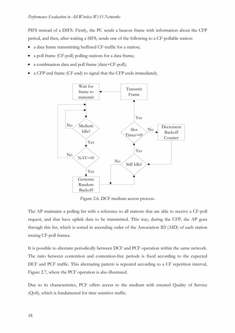
To finalise the discussion on DCF operation, Figure 2.6 represents the steps a station must go
through, in order to successfully transmit a frame.
Besides DCF, there is an optional access method based on a priority and centralised scheme. This
method, referred to as Point Coordination Function (PCF), provides a Contention-Free Period
(CFP) controlled by a centralised Point Coordinator (PC), which usually is the AP. This way, the
PCF is only implemented in an infrastructure BSS. Unlike DCF operation, the stations that are
able to work during the CFP period (referred to as CF-pollable stations) are not allowed to freely
access the medium and transmit data. They have to wait until the PC polls them.
At the beginning of a CFP, the PC gains control of the medium using DCF rules by waiting a
Performance Evaluation in All-Wireless Wi-Fi Networks
18
PIFS instead of a DIFS. Firstly, the PC sends a beacon frame with information about the CFP
period, and then, after waiting a SIFS, sends one of the following to a CF-pollable station:
a data frame transmitting buffered CF-traffic for a station;
a poll frame (CF-poll) polling stations for a data frame;
a combination data and poll frame (data+CF-poll);
a CFP end frame (CF-end) to signal that the CFP ends immediately.
Wait for
frame to
tramsmit
Medium
Idle?
NAV=0?
Generate
Random
Backoff
Still Idle?
Slot
Times=0?
Transmit
Frame
Decrement
Backoff
CounterYes
No
Yes
Yes
Yes
No
No
No
Figure 2.6. DCF medium access process.
The AP maintains a polling list with a reference to all stations that are able to receive a CF-poll
request, and that have uplink data to be transmitted. This way, during the CFP, the AP goes
through this list, which is sorted in ascending order of the Association ID (AID) of each station
issuing CF-poll frames.
It is possible to alternate periodically between DCF and PCF operation within the same network.
The ratio between contention and contention-free periods is fixed according to the expected
DCF and PCF traffic. This alternating pattern is repeated according to a CF repetition interval,
Figure 2.7, where the PCF operation is also illustrated.
Due to its characteristics, PCF offers access to the medium with ensured Quality of Service
(QoS), which is fundamental for time sensitive traffic.

802.11 Wireless LANs
19
Beacon D1+poll
SIFSPIFS
U1+ACK
SIFS SIFS
CF-end
Contention-Free Period Contention Period
Contention-Free Repetition Interval
D1 – Frame sent by
the point coodinator.
U1 – Frame sent by
polled station.
Figure 2.7. CF repetition interval.
2.2.2 MAC Frame Formats
All services provided by the MAC layer consist of well-defined frame sequences that allow a
meaningful exchange of information among stations.
There are three different types of MAC frames:
Control: these frames provide assistance during data frames exchange.
Management: these frames take care of several management services, essential for maintaining
a communication network.
Data: these frames carry station data between transmitter and receiver.
Each one of these frame types has several subtypes, described later in this section. All frame
types and subtypes are derived from the general IEEE 802.11 frame format, represented in
Figure 2.8. The MAC header of the general frame may seem too long; however, not all of these
fields are present in all frames, reflecting a trade off between efficiency and functionality.
Frame
Control
Duration
/IDAdress 1 Adress 2 Adress 3
Sequence
ControlAdress 4 Frame Body FCS
2 bytes 2 bytes 6 bytes 6 bytes 6 bytes 6 bytes0 - 2312
bytes2 bytes 4 bytes
Protocol
VersionType Subtype To DS
From
DS
More
Frag-
ments
Retry
Power
Mana-
gement
More
DataWEP Order
2 Bits 2 Bits 4 Bits 1 Bit 1 Bit 1 Bit 1 Bit 1 Bit 1 Bit 1 Bit 1 Bit
Figure 2.8. The general IEEE 802.11 MAC frame.

Performance Evaluation in All-Wireless Wi-Fi Networks
20
A description of all fields and subfields that compose the frame header is given in what follows:
Frame control: contains all the information that the MAC requires to correctly interpret all the
subsequent fields. As shown in Figure 2.8, it is made up of several subfields.
o Protocol version: specifies the version of the MAC protocol used to construct the frame.
To date, this subfield has only one valid value, since there is only one version.
o Type and subtypes: identify the function of the frame and which other MAC header fields
are present in the frame.
o To DS and From DS: indicate whether the frame is destined to the DS or comes from the
DS, respectively. When both subfields have a value of 0, the frame is directed from one
station to another, in the same IBSS. On the other hand, both subfields set to 1 indicate
that an IEEE 802.11 WLAN is being used as the DS.
o More fragments: indicates whether a frame is the last fragment of a larger frame or not.
o Retry: allows a receiver to realise if the frame is being retransmitted.
o Power management: used to announce the power management state of a station. If the
subfield is set to 1, the station enters in power save mode when the frame exchange is
completed. Frames from an AP always have a value of 0.
o More data: a station receiving a frame with the more data subfield set to 1 is notified that
there is at least one more data frame buffered at the AP.
o WEP: when set to 1, it indicates that the frame body has been encrypted using the Wired
Equivalent Privacy (WEP) algorithm.
o Order: indicates if the frame was provided to the MAC with a request for strictly ordered
service.
Duration/ID: the information contained in this field varies according to the state of the
station that is accessing the medium. Table 2.2 shows the different possible values for the
duration/ID field.
Address: each of these addresses contain one of the following subfields, depending on the to
DS and from DS subfields in the frame header, as shown in Table 2.3.
o BSS Identifier (BSSID): represents a unique identifier assigned to each BSS within an ESS.
o Transmitter Address (TA): MAC address of the station that transmits the frame.
o Receiver Address (RA): MAC address of the station to which the frame is sent over the
wireless medium.
o Source Address (SA): MAC address of the station that originates the frame.
Destination Address (DA): MAC address of the final destination of the frame.
Sequence control: sequence or fragment number of a frame.

802.11 Wireless LANs
21
Table 2.2. Values for the duration/ID field.
Duration/ID Field State of the station
Bit 15 Bit 14 Bit 13 – 0
0 0 – 32 767 DCF operation. Contains the duration of frame exchange (in microseconds), allowing other stations to update their NAVs.
1 0 0 PCF operation.
1 0 1 – 1683 Reserved.
1 1 0 Reserved.
1 1 1 – 2007 PS mode. Used in PS-poll frames to indicate the station AID.
1 1 2008 – 16 383 Reserved.
Table 2.3. Information contained in the different address fields.
To DS From DS Address 1 Address 2 Address 3 Address 4 Notes
0 0 RA=DA SA BSSSID - Frame exchange within an IBSS.
0 1 RA=DA BSSID SA - Frame from an AP.
1 0 RA=BSSID SA DA - Frame to an AP
1 1 RA TA DA SA IEEE 802.11 WLAN used as DS.
Frame body: this field carries the payload, or MSDU, of a frame delivered by upper layers.
There are several frames with an empty frame body. These are control frames, management
frames and the null data frame.
Frame check sequence (FCS): this field contains a 32-bit cyclic redundancy check (CRC) value
calculated over all fields in the MAC header and frame body.
As already mentioned, there are several frame subtypes for control, management and data frames.
A complete list of all of these frames is given below:
Control frames: PS-poll; RTS; CTS; ACK; CF-end; CF-end+CF-ACK.
Management frames: Beacon; Probe request; Probe response; Authentication;
Deauthentication; Association request; Association response; Reassociation request;
Reassociation response; Diassociation; Ad-hoc Traffic Indication Message (ATIM).
Data frames: Data; Null data; Data+CF-ACK; Data+CF-poll; Data+CF-ACK+CF-pool; CF-
ACK; CF-poll; CF-ACK+CF-poll.
Refer to [IEEE99] for a complete description of all frame subtypes.

Performance Evaluation in All-Wireless Wi-Fi Networks
22
Another important issue related to MAC frames is fragmentation. Basically, fragmentation is a
MAC function that brakes up a frame into smaller fragments, which are transmitted and
acknowledge individually. On the one hand, the effective throughput of the medium increases,
because if a collision occurs only a small fragment must be retransmitted, and not the entire
frame; on the other, the throughput decreases due to the higher overhead resulting from by an
increase of the number of headers and ACKs. Thus, fragmentation is a trade off between
medium reliability and medium overhead.
2.3 802.11 Physical Layer
To support all the functions of the MAC layer, described in the previous sections, there is the
need to define an underlying physical layer, which is also in the scope of 802.11 standards.
Besides this primary function, it is also responsible for other secondary ones, such as assessing
the state of the wireless medium and reporting it to the MAC. The following subsections present
a simple description of the existing physical layer specifications.
2.3.1 The Various Physical Layers
The basic function of the 802.11 PHY layer is to provide wireless transmission mechanisms for
the MAC layer. As described in Section 2.1, the PHY layer comprises two sublayers: the PLCP
and the PMD. While the former is responsible for mapping MPDUs frames, coming from the
upper MAC layer, onto an appropriate frame format, the latter provides adequate methods for
transmitting and receiving user data through a wireless medium. The PLCP sublayer can also be
seen as an interface between MAC and PMD, defining a set of primitives that enable
communication between the two adjacent layers. These primitives provide the interface for
transfer of data between the MAC and the PMD. Moreover, on transmission, there are primitives
that enable the MAC to tell PMD when to initiate transmission. On reception, PLCP primitives
indicate the start of an incoming transmission from another station to the MAC.
The IEEE 802.11 original standard has defined the MAC layer and three PHY layer
specifications, which are based on the following methods:

802.11 Wireless LANs
23
Direct Sequence Spread Spectrum (DSSS) operating in the 2.4 GHz Industrial, Scientific and
Medical (ISM) band, at data rates of 1 Mbps and 2 Mbps. DSSS WLANs use 22 MHz
channels that allow three non-overlapping channels in the 2.4 to 2.483 GHz range.
Frequency Hopping Spread Spectrum (FHSS) also operating in the 2.4 GHz ISM band, at the
same data rates. This technique uses 1 MHz channels and splits the available bandwidth into
79 non-overlapping channels.
Infrared at 1 Mbps and 2 Mbps, operating at a wavelength between 850 and 950 nm.
To overcome some limitations of the original PHY layer, several PHY specifications have been
issued: IEEE 802.11a [IEEE99a], 802.11b [IEEE99b] and 802.11g [IEEE03].
2.3.2 802.11a WLANs
IEEE 802.11a operates in the 5 GHz frequency band. It defines a set of 20 MHz channels within
the Universal Networking Information Infrastructure (UNII) band, which is divided into three
parts: the UNII-1 band (5.15 to 5.25 GHz), intended for indoor use; the UNII-2 (5.25 to
5.35 GHz), to be used for either indoor or outdoor; and the UNII-3 (5.725 to 5.825 GHz),
exclusively for outdoor use. The standard provides mandatory data rates up to 24 Mbps (6, 9, 12,
18 and 24 Mbps) and some optional rates up to 54 Mbps (36, 48 and 54 Mbps). 802.11a does not
use a spread spectrum scheme; instead, it uses Orthogonal Frequency Division Multiplexing
(OFDM), which uses multiple subcarriers for sending bits on each one.
The PLCP sublayer provides all the framing and signalling needed for PMD operations. It takes
the MPDUs coming from the upper MAC layer and adds some additional information, forming a
PLCP PDU (PPDU). Figure 2.9 illustrates the PPDU frame format.
The PLCP preamble enables the receiver to acquire an incoming signal and to synchronise the
demodulator. The signal field consists of the following subfields:
Rate: specifies the rate at which the subsequent data field will be transmitted.
r: reserved for future use.
Length: number of octets in the MPDU.
P: even parity bit.
Tail: provides six 0 bits for encoder use.

Performance Evaluation in All-Wireless Wi-Fi Networks
24
Rate r Length P Tail Service MPDU Tail Pad
DataSignalPLCP Preamble
12 OFDM symbols
1 OFDM
symbol Variable number of OFDM symbols
4
Bits
12
Bits
6
Bits16 Bits 6
Bits
1 1
Figure 2.9. IEEE 802.11a PPDU.
The preamble and signal fields are transmitted at the minimum data rate, i.e., 6 Mbps.
Subsequently, follows the transmission of the data field at the rate specified in the rate subfield.
Prior to transmission, the data field has to pass through a scrambling process. Besides the
MPDU, the data field consists of the following subfields:
Service: used to synchronise the scrambler at the receiver.
Tail: used for encoding purposes.
Pad: used to provide the remaining bits to make the data field a multiple of the number of bits
in an OFDM symbol.
Together with OFDM, the PMD sublayer supports several modulation and coding alternatives.
Each carrier is divided in up to 48 subcarriers that are modulated using BPSK, QPSK, 16-QAM
or 64-QAM. Table 2.4 shows the correspondence between available data rates and used
modulation.
Table 2.4. IEEE 802.11a data rates.
Data Rate [Mbps] Modulation
6 BPSK
9 BPSK
12 QPSK
18 QPSK
24 16-QAM
36 16-QAM
48 64-QAM
54 64-QAM
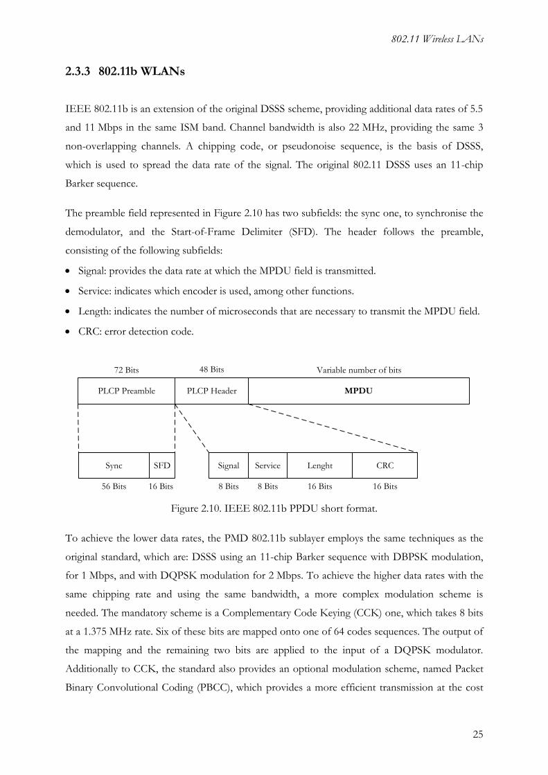
802.11 Wireless LANs
25
2.3.3 802.11b WLANs
IEEE 802.11b is an extension of the original DSSS scheme, providing additional data rates of 5.5
and 11 Mbps in the same ISM band. Channel bandwidth is also 22 MHz, providing the same 3
non-overlapping channels. A chipping code, or pseudonoise sequence, is the basis of DSSS,
which is used to spread the data rate of the signal. The original 802.11 DSSS uses an 11-chip
Barker sequence.
The preamble field represented in Figure 2.10 has two subfields: the sync one, to synchronise the
demodulator, and the Start-of-Frame Delimiter (SFD). The header follows the preamble,
consisting of the following subfields:
Signal: provides the data rate at which the MPDU field is transmitted.
Service: indicates which encoder is used, among other functions.
Length: indicates the number of microseconds that are necessary to transmit the MPDU field.
CRC: error detection code.
MPDUPLCP HeaderPLCP Preamble
72 Bits 48 Bits Variable number of bits
Sync SFD
56 Bits 16 Bits
Signal Service Lenght CRC
8 Bits 8 Bits 16 Bits 16 Bits
Figure 2.10. IEEE 802.11b PPDU short format.
To achieve the lower data rates, the PMD 802.11b sublayer employs the same techniques as the
original standard, which are: DSSS using an 11-chip Barker sequence with DBPSK modulation,
for 1 Mbps, and with DQPSK modulation for 2 Mbps. To achieve the higher data rates with the
same chipping rate and using the same bandwidth, a more complex modulation scheme is
needed. The mandatory scheme is a Complementary Code Keying (CCK) one, which takes 8 bits
at a 1.375 MHz rate. Six of these bits are mapped onto one of 64 codes sequences. The output of
the mapping and the remaining two bits are applied to the input of a DQPSK modulator.
Additionally to CCK, the standard also provides an optional modulation scheme, named Packet
Binary Convolutional Coding (PBCC), which provides a more efficient transmission at the cost

Performance Evaluation in All-Wireless Wi-Fi Networks
26
of increased computation requirements. Table 2.5 summarises the most important characteristics
of IEEE 802.11b.
Table 2.5. IEEE 802.11b.
Data Rate [Mbps] Chipping Code Length Modulation
1 11 (Barker sequence) DBPSK
2 11 (Barker sequence) DQPSK
5.5 8 (CCK) DQPSK
11 8 (CCK) DQPSK
2.3.4 802.11g WLANs
The IEEE 802.11g standard introduces an Extended Rate Physical (ERP) layer to support higher
data rates in the 2.4 GHz ISM band. The standard guarantees interoperability with the older
802.11b system, providing the same modulation and framing schemes for the lower data rates of
1, 2, 5.5 and 11 Mbps. Additionally, the 802.11g also provides a wide range of data rates: 6, 12
and 24 Mbps that are mandatory, and 9, 18, 36, 48 and 54 Mbps that are optional. To support
this additional data rates, a new modulation scheme is defined, referred to as ERP-OFDM. It is
also possible to optionally use a DSSS-OFDM scheme to support the same data rates and an
ERP-PBCC scheme to support 22 and 33 Mbps. Table 2.6 summarises some of the options in
terms of data rates and modulation schemes.
Table 2.6. IEEE 802.11g options.
Data Rate [Mbps] Modulation Scheme Data Rate [Mbps] Modulation Scheme
1 DSSS 18 ERP-OFDM
2 DSSS 22 ERP-PBCC
5.5 CCK or PBCC 24 ERP-OFDM
6 ERP-OFDM 33 ERP-PBCC
9 ERP-OFDM 36 ERP-OFDM
11 CCK or PBCC 48 ERP-OFDM
12 ERP-OFDM 54 ERP-OFDM
Five PPDU formats are provided, differing in the way the preamble is defined; three are
mandatory preambles (a long, a short, and an ERP-OFDM one), the remaining two, which are
optional, being the long and short DSSS-OFDM preambles.

802.11 Wireless LANs
27
An important figure when analysing WLANs performance or capacity is the relation between
distance and data rate. Since an RF signal experiences the decay of power while the distance to
the source increases, the available throughput decreases following a defined step function, thus,
the important capacity question is how far one can count on a particular data rate. The answer to
this question is not as straightforward as it may seem, and finding out the distance versus data
rate relation can be a complex issue. Different vendors provide different values, depending on
the environment. Table 2.7, based on [Layl04], gives estimated values for a typical office
environment with the maximum allowed power level.
Table 2.7. Estimated distance vs. data rate.
Data Rate [Mbps]
Distance [m]
802.11a 802.11b 802.11g
1 - 90 90
2 - 75 75
5.5 - 60 65
6 60 - 65
9 50 - 55
11 - 50 50
12 45 - 50
18 40 - 50
24 30 - 45
36 25 - 35
48 15 - 25
54 10 - 20
Note that the values in Table 2.7 are only an initial reference. Propagation in real environments,
possible occurrence of interferences from other sources, and the existence of multiple stations
using the same AP, contribute to the degradation of the presented values.
2.4 WLANs Backbone
As already mentioned in Section 2.1, the broadest topology for WLANs is the ESS. This
topology comprises several BSSs that are grouped via a DS. Although the services that are
provided by a DS are well-defined in the standard, their implementation is not specified. The

Performance Evaluation in All-Wireless Wi-Fi Networks
28
number of available possibilities is very high, since any type of data communication network can
be used. However, the most widely adopted implementation is the Ethernet LAN.
Of course, this perspective can be viewed the other way around, considering that one of the most
important applications of WLANs is the extension of wired LANs. In fact, WLANs are being
widely deployed as an extension of already existing wired LANs in locations where wiring is
difficult or not economical. Additionally, there are a number of other attractive characteristics of
WLANs, e.g., the flexibility on network modifications, and the possibility of nomadic access.
No matter what the initial perspective is, the fact remains that APs often appear coupled to a
wired backbone LAN. Therefore, this section focuses on the IEEE 802.3 standard [Stal00], being
based on the original Ethernet LAN technique, which is the most popular 802 LAN standard.
As all other IEEE 802 standards, 802.3 defines the MAC and the PHY layers of a LAN system.
Before considering these two layers in more detail, it is important to mention the two possible
topologies that are used to aggregate all the devices participating in the network: the bus and star
ones. While the former is characterised by a multipoint medium, where all stations attach, the
latter consists of a common central node (hub) that establishes point-to-point links with several
stations. Figure 2.11 represents these two topologies.
Ethernet
Hub
STAT2
STAT3
STAT1
Ethernet Bus
STAT1 STAT2 STAT3
a) Star b) Bus
Figure 2.11. IEEE 802.3 topologies.
IEEE 802.3 LAN being a broadcast network, that is to say when a station transmits all other
stations are able to receive, it must provide a fair access mechanism for all stations contending
the shared medium. This requirement is fulfilled by the MAC layer, which implements a CSMA
with Collision Detection (CSMA/CD); the principle of operation of CSMA/CD is quiet similar
to the one of CSMA/CA, which rules the medium access for WLANs. However, in the case of
an IEEE 802.3 LAN, there is no need for having such a stringent control mechanism, since

802.11 Wireless LANs
29
collision detection is easy to perform on a wired network. This way, the CSMA/CD operation
can be summarised as follows:
a station wishing to transmit first listens to the medium to determine if another transmission is
in progress (carrier sense);
if the medium is idle, it transmits;
if the medium is busy, it continues to listen until the channel is idle, and then transmits
immediately;
if a collision is detected during transmission, it stops transmitting and waits a random amount
of time, then, it attempts to transmit again.
An important rule followed in CSMA/CD systems is that frames should be long enough to allow
collision detection prior to the end of transmission. This fact must be taken into account in the
MAC frames definition.
The IEEE 802.3 standard provides a wide range of alternative PHY layer configurations to be
used with different transmission media. Basically, there are three reasons for having such an
extensive array of possibilities: keep the standard responsive to evolving technology; answer to
the increasingly demand of network capacity; and take advantage of already existing transmission
media (for instance, office buildings already wired with excess telephone cable).
All the PHY layer alternatives are grouped into three sets of specifications:
10 Mbps (Ethernet);
100 Mbps (Fast Ethernet);
1 Gbps (Gigabit Ethernet).
Some important features that characterise the most common implementations of each set of
specifications are presented in Table 2.8 to Table 2.10. The various implementations are labelled
according to the following IEEE 802.3 committee concise notation:
<data rate in Mbps> <signalling method> <maximum segment length in hundreds of meters>
The word BASE stands for Baseband, meaning that all the listed alternatives use Baseband
signalling techniques. In fact, all of them are encoding schemes that encode digital data into a
suitable digital signal. The details related with the signalling techniques, as well as the specific
characteristics of each transmission media, are out of the scope of this thesis. However, these
topics are extensively treated in literature, e.g., [Stal00].

Performance Evaluation in All-Wireless Wi-Fi Networks
30
Table 2.8. IEEE 802.3 10 Mbps PHY layer alternatives.
Implementation Data rate [Mbps]
Transmission media Signalling technique
Maximum segment length [m]
10BASE5 10 Coaxial cable (50 Ω) Manchester 500
10BASE2 10 Coaxial cable (50 Ω) Manchester 185
10BASE-T 10 Unshielded twisted pair
(UTP) Manchester 100
10BASE-FP 10 850 nm optical fiber pair Manchester/
on-off 500
Table 2.9. IEEE 802.3 100 Mbps PHY layer alternatives.
Implementation Data rate [Mbps]
Transmission media Signalling technique
Maximum segment length [m]
100BASE-TX 100
2 pair, shielded twisted pair (STP)
MLT-3 100
2 pair, Category 5 UTP MLT-3 100
100BASE-FX 100 2 optical fibers 4B5B, NRZI 100
100BASE-T4 100 4 pair, Category 3, 4 or 5
UTP 8B6T, NRZ 100
Table 2.10. IEEE 802.3 1 Gbps PHY layer alternatives.
Implementation Data rate [Gbps]
Transmission media Signalling technique
Maximum segment length [m]
1000BASE-SX 1
62.5 µm multimode optical fiber
8B/10B 275
50 µm multimode optical fiber
8B/10B 550
1000BASE-LX 1
62.5 µm or 50 µm multimode optical fiber
8B/10B 550
10 µm single-mode optical fiber
8B/10B 5000
1000BASE-CX 1 STP 8B/10B 25
1000BASE-T 1 4 pair, Category 5 UTP 8B/10B 100
The maximum allowed length for a cable segment in an IEEE 802.3 LAN is obtained
considering several factors, as for instance, the restrictions imposed to allow collision detection.
Besides the typical perspective that has been discussed in the present section, which consists of
viewing a WLAN as a set of APs that connect to the access layer of a LAN, there are other
common WLAN deployment scenarios. One that is becoming very popular is the use of APs to
support broadband access of the general public to the Internet, via the wireless medium and in

802.11 Wireless LANs
31
particular areas, usually referred to as “hot spots”. Actually, during the past few years, thousands
of hot spots have already been deployed, and this number is increasing. Dozens of APs have
been installed at hotels, airports, restaurants, bookstores, schools, theatres, convention centres,
health clubs, and other public venues.
The use of WLANs to provide public access to broadband Internet raises some specific issues,
e.g., in the area of authentication and billing. However, the basic configuration is quite simple,
consisting of an AP that supports roaming to other networks connected to the Internet [Vars03].
The available data rate for each client station depends on the WLAN characteristics, but it is also
limited by the network to which the AP is connected.
There are a number of available technologies providing broadband access to Internet. Currently,
the most prominent ones are:
Asymmetric Digital Subscriber Line (ADSL);
cable modem;
satellite based networks;
third-generation cellular networks;
Power Line Communications (PLC).
Among all these possibilities, the most popular one is ADSL, having a worldwide market share
greater than 60 %, [DSLF07].
ADSL is a technology designed to provide high-speed digital data transmission over ordinary
telephone wires (e.g., UTP), which were installed to carry voice signals in a bandwidth up to
4 kHz. However, they have a far broader capacity of 1 MHz, which is exploited by ADSL using a
frequency division modulation technique. The lowest 25 kHz band is reserved for voice, while
the remaining bandwidth is further subdivided into a smaller upstream band (25 to 200 kHz) and
a larger downstream one (250 kHz to 1 MHz). This asymmetric division of resources fits well in
Internet requirements, were downstream traffic (from the carrier’s central office to the
customer’s site) may involve large amounts of data and include images or even video. The ADSL
scheme provides a range up to 5.5 km, depending on the diameter of the cable and its quality
[Stal00].
The underlying technology of ADSL is Discrete Multitone (DMT), which consists of using
multiple carrier signals at different frequencies, each one carrying some bits of the total stream to
be transmitted. The available transmission band (upstream or downstream) is divided into a
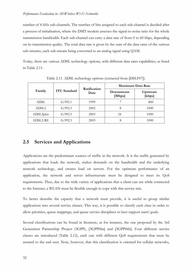
Performance Evaluation in All-Wireless Wi-Fi Networks
32
number of 4 kHz sub-channels. The number of bits assigned to each sub-channel is decided after
a process of initialisation, where the DMT modem assesses the signal-to-noise ratio for the whole
transmission bandwidth. Each sub-channel can carry a data rate of from 0 to 60 kbps, depending
on its transmission quality. The total data rate is given by the sum of the data rates of the various
sub-streams, each sub-stream being converted to an analog signal using QAM.
Today, there are various ADSL technology options, with different data rates capabilities, as listed
in Table 2.11.
Table 2.11. ADSL technology options (extracted from [DSLF07]).
Family ITU Standard Ratification
Date
Maximum Data Rate
Downstream [Mbps]
Upstream [kbps]
ADSL G.992.1 1999 7 800
ADSL2 G.992.3 2002 8 1000
ADSL2plus G.992.5 2003 24 1000
ADSL2-RE G.992.3 2003 8 1000
2.5 Services and Applications
Applications are the predominant sources of traffic in the network. It is the traffic generated by
applications that loads the network, makes demands on the bandwidth and the underlying
network technology, and creates load on servers. For the optimum performance of an
application, the network and server infrastructure must be designed to meet its QoS
requirements. Thus, due to the wide variety of applications that a client can use while connected
to the Internet, a WLAN must be flexible enough to cope with this service mix.
To better describe the capacity that a network must provide, it is useful to group similar
applications into several service classes. This way, it is possible to classify each class in order to
allow priorities, queue mappings, and queue service disciplines to best support users’ goals.
Several classifications can be found in literature, as for instance, the one proposed by the 3rd
Generation Partnership Project (3GPP), [3GPP06a] and [3GPP06b]. Four different service
classes are introduced (Table 2.12), each one with different QoS requirements that must be
assured to the end user. Note, however, that this classification is oriented for cellular networks,

802.11 Wireless LANs
33
which are in many aspects different from WLANs.
The Conversational class is the most symmetric one, the amount of downlink traffic flow being
very similar to the uplink one. The remaining classes are not characterised by this symmetry, since
downlink traffic is much higher than uplink one, which is originated mainly by client requests to
servers. The distinction between client-to-client (also known as peer-to-peer) and client-to-server
applications is apparent, Figure 2.12. Data exchange, or conversation, consists in a client issuing a
request and a server or client returning a response. A conversation includes a pattern, typically
defined in a statistical manner that repeats over time.
Table 2.12. 3GPP Service Classes (adapted from [3GPP06a] and [3GPP06b]).
Class Characteristics Class
Conversational Streaming Interactive Background
Real-time Yes Yes No No
Symmetric Yes No No No
Assured throughput Yes Yes No No
Delay Minimum and
fixed Minimum and
variable Moderate and
variable Large and variable
Conversation
Client1
a) Client-to-Client
Client2
Request
Response
Request
Response
Conversation
Client
b) Client-to-Server
Request
Response
Server
Figure 2.12. Data exchange definition (adapted from [OPMo06]).
Another important characteristic that distinguishes the Conversational class from the others is
the requirement of low end-to-end delays, in order to keep a communication perceptible at both
ends (voice and video conferencing are good examples to illustrate the importance of this
requirement).
Another service classification is provided by the 802.1D standard [IEEE04], which is more
oriented to WLANs. Seven service classes are defined, in decreasing order of priority:
Network Control – Represents the traffic necessary to maintain and support the network
infrastructure.

Performance Evaluation in All-Wireless Wi-Fi Networks
34
“Voice” – Characterised by requiring very low delays.
“Video” – Also requires low delays, but is not as stringent as previous class.
Controlled Load – Represents applications with some sort of admission control and with
controlled throughput.
Excellent Effort.
Best Effort – Typical LAN traffic.
Background – Characterises activities that are permitted on the network, but that should not
impair the use of the network by other applications.
The expression service mix, used at the beginning of this section, stands for the traffic that flows
throughout a network, being generated by users running applications of different service classes.
To have such a mix, with the presence of all service classes defined above, the following
commonly-used applications can be selected:
FTP (File Transfer Protocol);
E-mail;
Web Browsing;
Video Streaming;
Video Conferencing;
VoIP (Voice over Internet Protocol (IP)).
An FTP application enables file transfers between a client and a server, using two basic
commands: “get” and “put”. While the “get” command triggers the transfer of a file from a
remote server, the “put” command sends a file to it. For each commanded file transfer, the FTP
application sends a control message and a data message, using a single Transmission Control
Protocol (TCP) connection.
The common E-mail packages use a combination of Simple Mail Transfer Protocol (SMTP) and
Post Office Protocol (POP). Usually, the default transport protocol is TCP.
Traffic generated by Web Browsing applications essentially results from clients downloading
pages from a remote server. Pages can contain text and graphic information (also referred to as
“inline objects”). Note that each page request may result in multiple TCP connections, allowing
the transfer of inline objects embedded in the page.
Video Streaming is characterised by a main unidirectional stream with limited end-to-end delay.

802.11 Wireless LANs
35
This requirement is not very stringent due to the existence of buffers, which can cope with delay
variations. Thus, for the sake of convenience, Video Streaming is classified during the present
study as a non-real time application.
The flexibility in terms of end-to-end delay that characterises the previous applications is not
allowed in Video Conferencing, which is an example of a time-based application. A continuous
sequence of data blocks must be received by the client at a pre-determined order and at
pre-defined instants.
A voice application, as VoIP, enables two clients to establish a virtual channel over which they
can communicate using encoded voice signals. Voice data arrives in spurts that are followed by a
silence period.
Independently of the service classes that can be defined, the existence of two broadest
application types is evident: non-real time centric (FTP, E-mail, Web Browsing, and Video
Streaming) and real time centric (Video Conferencing and VoIP).
Modelling the traffic flow generated by each application can be a complex task, requiring the
consideration of several attributes and settings. All the necessary attributes for each application
are listed in Annex A, together with a detailed description.
Finally, and to assess the overall performance of every application, it is important to define a set
of evaluation metrics:
FTP Download Response Time (RTFTP): Time elapsed between sending a request and
receiving the response packet, measured from the time a client application sends a request to
the server to the time it receives a response packet.
E-mail Download Response Time (RTmailD): Time elapsed between sending request for e-mails
and receiving them from e-mail server in the network. This time includes signalling delay for
the connection setup.
E-mail Upload Response Time (RTmailU): Time elapsed between sending e-mails to the e-mail
server and receiving acknowledgments from the email server. This time includes signalling
delay for the connection setup.
Web Browsing Page Response Time (RTweb): Time required to retrieve the entire page with all
the contained inline objects.
Video Streaming and Video Conferencing Packet End-to-End Delay (Evideo): The time taken to
send a video application packet to a destination node application layer.

Performance Evaluation in All-Wireless Wi-Fi Networks
36
VoIP Packet End-to-End Delay (EVoIP): The total voice packet delay, called "analog-to-analog"
or "mouth-to-ear" delay, which is computed by summing the following delays: Network delay
(time at which the sender node gave the packet to physical layer to the time the receiver got it
from the same layer); Encoding delay on the sender node (computed from the encoder
scheme); Decoding delay on the receiver node (assumed to be equal to the encoding delay);
Compression and Decompression delays.
From the above statistics, EVoIP is the one with strictest requirements. In fact, values above
200 ms [ITUT03] are not considered acceptable to maintain a VoIP connection able to provide
an appropriate quality to end users.
Response times of non-real time application do not have stringent requirements, being subjected
to users’ expectations. Thus, analysis of these parameters is considered in relative terms,
comparing the results obtained at different scenarios.

Simulations of WLANs with Wireless Backbone
37
Chapter 3
Simulations of WLANs
with Wireless Backbone
3 Simulations of WLANs with Wireless Backbone
This chapter provides the rationale behind the simulations conducted within the present study. It
starts with an introduction to wireless backbone issues as the background to the implementation
model setup, associated with thesis objectives. Then, it gives a general overview of the selected
simulation tool and details about specific models for WLANs. Finally, it describes how these
models are combined to implement the scenario that is the basis of all simulation runs.

Performance Evaluation in All-Wireless Wi-Fi Networks
38
3.1 WLANs with Wireless Backbone
In order to introduce the discussion on wireless backbones, Section 3.1.1 begins by pointing out
the main issues related to mesh networks, while presenting a review of the available literature on
each of them. Then, a brief description of commercial solutions that are already available is
presented, as well as the standardisation efforts that are being conducted within IEEE. Note that
Section 3.1.1 can be viewed as an extension of Section 2.4, providing a description of another
possibility for a DS implementation. Having established the appropriate background, Section
3.1.2 puts the objective of the present work into context, by setting up the simulation
environment and all adopted options.
3.1.1 Related Work
In the past few years, wireless mesh networks have been widely studied by the scientific
community, [AkWa05]. Many related works can be found in the literature, focusing on several
key functionalities, performance parameters and implementation problems of mesh networks.
This generalised effort is being motivated by the increasing demand on extending the coverage
range of WLANs, interconnecting APs through a wireless link, which, in other words, can be
described as the creation of mesh networks based on 802.11.
When implementing or analysing a wireless mesh network, it is necessary to consider several key
issues, in order to obtain satisfactory results. As described in the following paragraphs, these
issues can include backbone networking, mesh topology creation, routing, security and QoS.
Note that the backbone of a wireless mesh network has the characteristics of multihop
transmissions, thus, studies specifically related to multihop networks can also be considered in
the context of mesh networks.
Within backbone networking, there are several proposed solutions in terms of the number of
radio interfaces installed in each MAP, and also in terms of radio channels usage. Figure 3.1
depicts the 3 basic approaches to wireless mesh networks.
The single radio approach is the weakest one. It uses only one radio on a single channel in the
AP, shared by wireless clients and backbone traffic (forwarded between APs). It is easy to
understand that the more APs are added the more channel capacity is dedicated to backbone

Simulations of WLANs with Wireless Backbone
39
traffic, very little capacity remaining to support clients.
The use of two radios in the dual radio approach, one for client support and another for
backbone, represents an improvement compared to single radio. However, wireless backbone is
still a shared network, also subjected to network contention issues.
Like the dual radio wireless mesh, the multi radio approach separates access and backbone, but it
goes a step further, by allowing links between different APs that can transmit and receive
simultaneously on separate channels. Backbone mesh is no longer a shared network.
a) Single Radio
AP
AP
AP
AP
AP
AP
AP
AP
AP
b) Dual Radio c) Multi Radio
Same channel for access
and backbone
One channel for access
and other for backbone
One channel for access
and several for backbone
Figure 3.1. Basic approaches to wireless mesh networks.
Several interesting works exploring different questions related to the above approaches can be
found in literature. Most of them consist of new MAC schemes proposals, aiming at taking
advantage of the several channels that are available in the ISM band. As an example, [FAMZ03]
introduces a dynamic mechanism for the choice of transmission channels. The new MAC scheme
is based on the use of a common signalling channel and several different dedicated channels to
carry traffic. The assignment of dedicated channels is conducted by a four-handshake procedure
with the use of two RTS/CTS transmissions over the common signalling channel. Regarding the
use of multiple radios interfaces, [RaCh05] and the references therein provide good examples of
possible approaches. The authors describe an 802.11 multihop network architecture (called
Hyacinth) that employs multiple radio channels simultaneously by equipping each node with

Performance Evaluation in All-Wireless Wi-Fi Networks
40
multiple NICs. Simulation results show that, by using just 2 NICs per node, it is possible to
achieve an improvement of throughput (by a factor of 6 to 7), compared to the conventional
single-channel architecture.
In addition to new proposals, as the ones referred above, there are also several works dedicated
to the identification of 802.11 MAC problems over multihop and mesh networks. A well known
reference is [XuSa04], which revealed some of the CSMA/CA problems by using TCP as the
transport layer protocol to evaluate the throughput performance. Simulation results show
instability and unfairness among TCP connections mainly caused by the hidden node and the
exposed terminal problems. Following similar approaches, [HsSi02] and [TsCh05] also conclude
that the 802.11 MAC protocol does not fit the requirements of mesh networks.
Upon activation, Mesh Points (MPs) need to discover mesh networks that may be already present
in their vicinity. When a network is detected, MPs must be able to associate to it, otherwise, they
need to be capable of initiating a new one. This process is part of the mesh topology creation
[FWKD06]. Due to their characteristics, mesh networks functionality does not end in the
topology creation phase. They must be able to move a step further and deal with topology
maintenance. Each node needs to obtain information about the current state of the topology, in
order to refresh its connectivity associations and update them when necessary (for instance, due
to mobility).
Most of the backbone topology creation algorithms that are available in the literature have been
designed for ad hoc networks. In such networks, all nodes use a single radio module that is
operated across a single common frequency band, thus, the referred algorithms do not fully
explore all the mesh networks potentialities. Nevertheless, a few studies considering the use of
multiple radio modules at a device and multiple communication channels can be found, e.g.,
[JuRu06]. Here, the authors propose a scalable and fully distributed Multi-Radio Backbone
Synthesis Algorithm (MR-BSA) that is used for constructing and maintaining the backbone of a
mesh network. It is considered that a mesh network is made of Backbone Capable Nodes
(BCNs) and Regular Nodes (RNs), depending on their processing and transmission capabilities.
The backbone network is formed by dynamically electing BCNs to act as backbone nodes (BNs),
which interconnect with other BNs in the neighbourhood. The algorithm aims at selecting a
sufficient but not excessive number of BNs, while providing high coverage.
One of the most important issues in mesh network investigation is routing, which is essential to
allow communication among MPs [FWKD06]. Reflecting this importance, in the past few years a

Simulations of WLANs with Wireless Backbone
41
lot of work has been done on routing protocols suitable for wireless ad hoc networks. One
important contributor for this effort has been the IETF MANET [IETF07] working group,
which concentrates its activity on standardising IP (layer 3) routing protocol functionalities.
However, layer 3 routing may not directly apply to mesh networks needs. This type of networks
is composed of mesh stations and also of MAPs, which traditionally are purely layer 2 devices,
thus, being incapable of decoding IP packets. Since adding layer 3 functionality to APs is typically
considered unacceptable, routing in 802.11 mesh networks has to be performed at layer 2 level,
or, in other words, routing has to be based on MAC addresses.
The determination of the preferred route between source and destination is achieved with the
help of evaluation metrics. In order to provide efficient routing and support complex mesh
networks, it is necessary to consider an extended set of metrics, besides the conventional “hop
count”. This set may include [FWKD06]: QoS parameters, power efficiency, security of wireless
links and intermediate nodes, reliability, etc..
Just to give an example, [JuRu06] presents a routing protocol that tries to reduce the amount of
Route Request (RREQ) packets (typical of protocols for ad hoc networks) broadcasted across the
entire network. The aim of this approach is to increase scalability of existing protocols.
Another key issue in the design of mesh networks is security. Efficient solutions for
authentication and encryption are expected to be based on the use of 802.11i standard
[FWKD06].
Finally, QoS mechanisms must also be considered in the context of mesh networks. In addition
to the existence of applications with QoS requirements, it is necessary to differentiate between
access network traffic and backbone one, in order to obtain the appropriate service level
[FWKD06]. For inter-MP traffic, the MAC layer is able to guarantee a minimum service level by
means of different interframe spaces for access and backbone traffic, or by means of service
differentiation mechanisms (802.11e). Another interesting solution is given in [ZhWH06], where
MPs use time division techniques. The proposed MAC protocol for interconnecting APs is called
Mesh Distributed Coordination Function (MDCF), being based on Time Division Multiple
Access/Time Division Duplex (TDMA/TDD) technology. In general terms, with MDCF an MP
contends for channel access to reserve a number of periodic TDMA slots for data transmission,
according to QoS requirements. If successful, the reserved time slots form the link to connect
two MPs in the TDD mode of operation to multiplex all packets having the link in their route.

Performance Evaluation in All-Wireless Wi-Fi Networks
42
In addition to this type of works, proposing new MAC schemes to guarantee QoS, it is also
possible to find in literature several studies evaluating the performance of current 802.11
standards when supporting applications with QoS requirements. One example is [VaHa05],
which evaluates VoIP usage over a multihop 802.11b WLAN. Via simulations, the authors have
concluded that this type of networks cannot support a large number of random VoIP
connections.
Despite all the challenges and open issues remaining in literature, several commercial solutions
are already available in the market, e.g.: [BeAr07], [Fire07], [MhDy06], [PkHo07], [StSy07] and
[Trop07], just to list a few. Most of them try to deploy solutions that are self-forming (network
automatically formed upon powering up), self-configuring and self-healing (backbone radios
switch channels automatically, depending on channel characteristics). All proposals provide
proprietary solutions to comply with mesh networks requirements, e.g., routing protocols are
proposed by each vendor.
To take advantage of the increased capacity achieved when using multiple radios, [MhDy06] and
[StSy07] provide mesh routers equipped with several radios interfaces. In addition, mesh nodes
from [Fire07] can be configured with directional antennas to achieve longer ranges or to
minimise wireless interferences. Moreover, [BeAr07] provides the interesting possibility to
integrate radio modules for WiMAX and GSM.
Such proprietary approaches work satisfactorily in certain conditions, if all devices in the network
are provided by the same manufacturer. To overcome this problem, the IEEE 802.11 working
group has established the 802.11s TGs, which is chartered to develop an additional amendment
to the existing 802.11 MAC to realise mesh networks. Essentially, the main objective is to make
the DS wireless over self-configuring multihop topologies.
At the moment this thesis is being written, TGs is evaluating the several proposals that have been
issued. All proposals recognise that wireless mesh networks are networks that are not fully
managed by a service provider, thus, needing to be self-configurable. The multiple aspects that
must be considered are [IEEE07a]:
basic MAC extensions;
topology discovery and channelisation proposals;
routing proposals (a layer 2 routing approach will be introduced);
additional extensions (as for instance, use of multiple radio devices).

Simulations of WLANs with Wireless Backbone
43
It is likely that the 802.11s amendment will provide a sort of “default” configuration regarding
the several topics mentioned above. Additionally, vendors will have the possibility to implement
enhanced versions to address some particular aspect of the new standard.
3.1.2 Performance Analysis of a Wireless Backbone
As described in the previous subsection, several studies in literature have shown that the
integration of multiple radio interfaces within a single device can improve performance and
capacity of wireless mesh networks. This represents a general improvement to the most
restrictive solution of considering a network formed only by single radio, single channel nodes. In
fact, equipping MAPs with multiple radio interfaces allows simultaneous transmission between
MAPs and clients (access network), and among MAPs (backbone network), via the use of
different channels. This possibility is implemented by algorithms of channel selection, which
automatically select channels based on certain parameters, e.g., RF channel characteristics.
Reflecting the importance of such algorithms, several studies in literature and also several
commercial solutions address the issue of automatic channel selection (refer to Subsection 3.1.1
and references therein).
To reduce even more interference among simultaneous transmissions, there is also the possibility
to select channels among different frequency bands. The most common approach is to use a
frequency band for client access (for example, the 2.4 GHz IEEE 802.11b/g band) and another
for backbone (for example, the 5 GHz IEEE 802.11a band). Despite several vendors already
provide solutions using multiple radios and multiple frequency bands ([BeAr07] and [MhDy06],
for instance), there is still a number of open issues on this alternative to provide a wireless
backbone in the context of an All-Wireless network. From the point of view of the present study,
they are:
The selection of technologies (and thus of frequency bands) to use within a mesh network,
which is performed at network set up. Usually, the criteria for this selection are based on
capacity and reduction of RF interference between adjacent connections. Nevertheless, there
are other metrics that can be used, e.g., the presence, or not, of traffic with QoS requirements.
The number of stations associated to each MAP, as well as the distance between MAPs, are
important parameters, since they can constrain the global performance of such a network.
Thus, knowing the maximum values that they can assume without any performance

Performance Evaluation in All-Wireless Wi-Fi Networks
44
degradation will help on taking some decisions during network set up and operation. Note
that the maximum value of distance can be used (with some assumptions) for the calculation
of a minimum MAPs density.
From the wide range of data rates provided by 802.11 standards, it is important to know
which ones can be used without impairing the overall performance.
Some internal MAPs parameters can also play an essential role in network performance, as for
instance buffer size. Thus, there is a need to investigate in which particular conditions it will
influence performance.
In general terms, these issues represent the guideline of the present study. Moreover, it is always
considered a worst case perspective to provide boundary values for the above mentioned
parameters, in order not to have degradation in network performance. Having this in mind, the
following paragraphs are dedicated to develop an adequate implementation scenario, and to select
a set of evaluation statistics.
In order to separate the influence of RF interference between adjacent connections from other
network parameters, the implementation scenario contains just two MAPs. Moreover, to
guarantee that all generated traffic passes through the backbone network, all clients are associated
to one MAP, while all servers are associated to the other. Figure 3.2 represents this scenario,
where:
RI stands for radio interface;
N is the number of clients associated to MAP1;
M is the number of servers associated to MAP2;
BSS0 is the basic service set composed of both MAP1 and MAP2 RI2;
BSS1 is the basic service set composed of MAP1 RI1 and all the N client stations;
BSS2 is the basic service set composed of MAP2 RI1 and all the M servers.
This implementation scenario has several degrees of freedom (parameters that can assume
different values), which can be used to investigate some aspects of the backbone network (BSS0).
From the point of view of this study, they are:
Technology used in BSS0 (802.11a, b or g);
Applications Distribution (AD), which represents the assignment of applications (refer to
Section 2.5) to client stations; variation of this degree of freedom delivers different traffic
patterns to BSS0;
distance between MAP1 and MAP2 (D);

Simulations of WLANs with Wireless Backbone
45
number of clients associated to MAP1 – N;
nominal data rate (RN) in BSS0;
MAP1 and MAP2 buffer size (Bf).
RI2
CLIENT1R
I1 MAP1CLIENT2
CLIENTN
CLIENT3
MAP2
SERVER1
RI2
RI1
SERVER2
SERVERM
BSS1 BSS2BSS0
Figure 3.2. Implementation model.
The methodology adopted during the study consists of varying two degrees of freedom
simultaneously, while the remaining ones are fixed in a pre-selected value. In order to compare
the results obtained with different technologies in BSS0, this is always one of the changing
degrees of freedom.
To study the performance of the backbone network (BSS0), one has to identify a set of adequate
evaluation metrics. They are used to quantify this generic term of performance, allowing the
comparison of results from several simulation runs. The ones that best fit this aim, considering
the described scenario, are listed below. All of them are collected on both MAP1 and MAP2 RI2:
Throughput (R) – Total data traffic successfully received and forwarded to the higher layer by
the MAC.
Retransmission attempts (RTX) – Number of retransmission attempts until either the packet is
successfully transmitted or it is discarded as a result of reaching the retransmission threshold.
Media access delay (TDL) – The total of queuing and contention delays of data packets received
by the MAC from higher layer.
Queue Size (Q) - Size of the queue that holds the frames received from higher layer until their
transmission is completed. In stations operating as access points, the queue size represented

Performance Evaluation in All-Wireless Wi-Fi Networks
46
by this statistic also includes the frames that are received from physical layer and awaiting
being forwarded to their final destination within the AP's BSS.
Data dropped due to buffer overflow (Dbuf) – Higher layer data traffic dropped by the MAC
due to: full higher layer data buffer, or the size of the higher layer packet, which is greater than
the maximum allowed data size defined in the IEEE 802.11 standard.
Data dropped due to retransmission threshold exceeded (Drtx) – Higher layer data traffic
dropped by the MAC due to consistently failing retransmissions. This statistic reports the
number of the higher layer packets that are dropped because the MAC could not receive any
ACKs for the (re)transmissions of those packets or their fragments, and the packets' retry
counts reached the MAC's retry limit.
Additionally, all evaluation metrics described in Section 2.5 are also considered. This way, it is
possible to quantify the effect of varying network parameters on applications running in the
client stations.
3.2 OPNET Modeler Basics
OPNET Technologies [OPNT07] is a leading provider of management software for networks
and applications. Its solutions provide analysis of the behaviour of applications, networks and
systems. OPNET simulation tools are used worldwide by a large number of costumers, ranging
from IT enterprises and service providers to governmental agencies and R&D organisations.
From all available tools, there is one that is fully adequate to investigate the impact of using a
wireless backbone in a WLAN design. That tool is OPNET Modeler, which is the focus of this
section. A detailed explanation on the complete portfolio of OPNET tools is available at
[OPNT07].
3.2.1 Initial Considerations
Modeler incorporates a vast suite of protocols and technologies, including a development
environment to enable the modelling of all network types and technologies. Moreover, together
with the Modeler Wireless Module, it allows the analysis of a broad range of wireless network
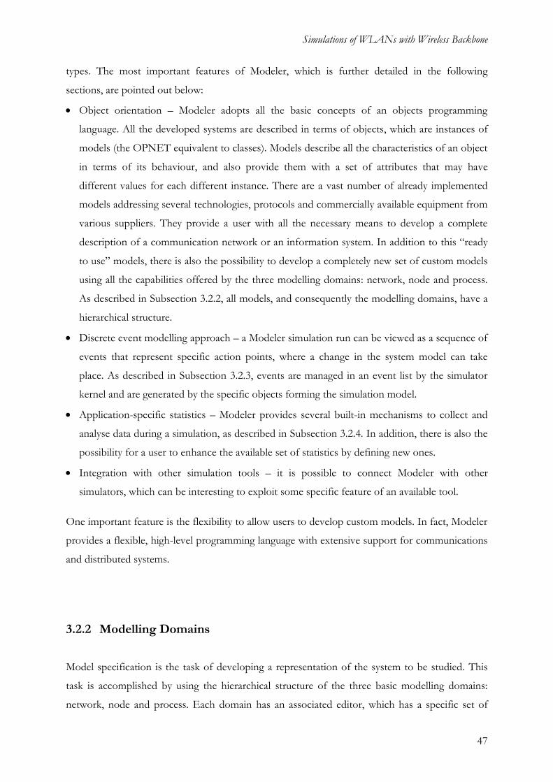
Simulations of WLANs with Wireless Backbone
47
types. The most important features of Modeler, which is further detailed in the following
sections, are pointed out below:
Object orientation – Modeler adopts all the basic concepts of an objects programming
language. All the developed systems are described in terms of objects, which are instances of
models (the OPNET equivalent to classes). Models describe all the characteristics of an object
in terms of its behaviour, and also provide them with a set of attributes that may have
different values for each different instance. There are a vast number of already implemented
models addressing several technologies, protocols and commercially available equipment from
various suppliers. They provide a user with all the necessary means to develop a complete
description of a communication network or an information system. In addition to this “ready
to use” models, there is also the possibility to develop a completely new set of custom models
using all the capabilities offered by the three modelling domains: network, node and process.
As described in Subsection 3.2.2, all models, and consequently the modelling domains, have a
hierarchical structure.
Discrete event modelling approach – a Modeler simulation run can be viewed as a sequence of
events that represent specific action points, where a change in the system model can take
place. As described in Subsection 3.2.3, events are managed in an event list by the simulator
kernel and are generated by the specific objects forming the simulation model.
Application-specific statistics – Modeler provides several built-in mechanisms to collect and
analyse data during a simulation, as described in Subsection 3.2.4. In addition, there is also the
possibility for a user to enhance the available set of statistics by defining new ones.
Integration with other simulation tools – it is possible to connect Modeler with other
simulators, which can be interesting to exploit some specific feature of an available tool.
One important feature is the flexibility to allow users to develop custom models. In fact, Modeler
provides a flexible, high-level programming language with extensive support for communications
and distributed systems.
3.2.2 Modelling Domains
Model specification is the task of developing a representation of the system to be studied. This
task is accomplished by using the hierarchical structure of the three basic modelling domains:
network, node and process. Each domain has an associated editor, which has a specific set of

Performance Evaluation in All-Wireless Wi-Fi Networks
48
objects and operations for the modelling task on which it is focused.
The first hierarchical level is the network domain with its associated project editor, Figure 3.3.
This editor has a central role on all the graphical interfaces of Modeler. Using the project editor, a
user can define the topology of an entire communications network, by deploying node and link
objects that are instances of models developed in the lower levels.
Nodes
Links
Figure 3.3. Project editor (network domain) with an example of a network model.
In order to break down the complexity of large networks, models make use of an abstraction
known as subnetwork. A subnetwork can be viewed as a network in its own right, with its own
nodes and links, and can be included on a larger network as a simple node. This abstraction can
be carried out at many levels, but at the bottom of this hierarchy there can be only nodes and
links, and no other subnetwork.
As already mentioned, Modeler comes with a wide range of already implemented node models.
Figure 3.4 depicts just a few of them.
The node models that can be interconnected at the network level are developed at the second
hierarchical level, the node domain. Node models are developed in the node editor and consist of
small functional elements (modules) and the connections among them. As an example, Figure 3.5
shows the wlan_wkstn node model internal structure. This model represents a workstation with

Simulations of WLANs with Wireless Backbone
49
client-server applications running over TCP/IP or UDP/IP, supporting an underlying WLAN
connection. Each module controls the behaviour of the specific capabilities and protocols
implemented in the node. For example, the wireless_lan_mac module is the implementation of
the 802.11 MAC layer.
Figure 3.4. Some node models representations.
Node Editor
Modules
Data Flow
Between Modules
Figure 3.5. Example of a node model description.
Some modules offer capabilities that are predefined and can only be configured through a set of
specific parameters, which include various transmitters and receivers that are responsible for the
connection with communication links in the network domain. Other modules (processors and
queues) are highly programmable, with their behaviour being described by an assigned process
model, as described later in this section. Figure 3.6 shows some examples of the referred

Performance Evaluation in All-Wireless Wi-Fi Networks
50
modules.
Figure 3.6. Examples of modules available at node domain.
Figure 3.7 illustrates the three types of connections that can be used to support interaction
among the various modules within a node. Packet streams allow the flow of packets between
modules. Statistic wires transmit simple control information between modules, being typically
used when one module needs to know the state of another. Logical associations are only used to
connect a receiver to a transmitter, indicating that they should be used as a pair when attaching
the node to a link in the network domain.
Packet
Stream
Statistic
Wire
Logical
Association
Figure 3.7. Connections between modules in the node domain.
As already mentioned, processors and queues are user-programmable modules that can perform
any specific task within a node, called processes, which are instances of a process model. The
relationship between a process model and a process is similar to the relationship between a
program and a particular session of that program running as a task.
The specification of a process model is performed at the bottom of the modelling hierarchical
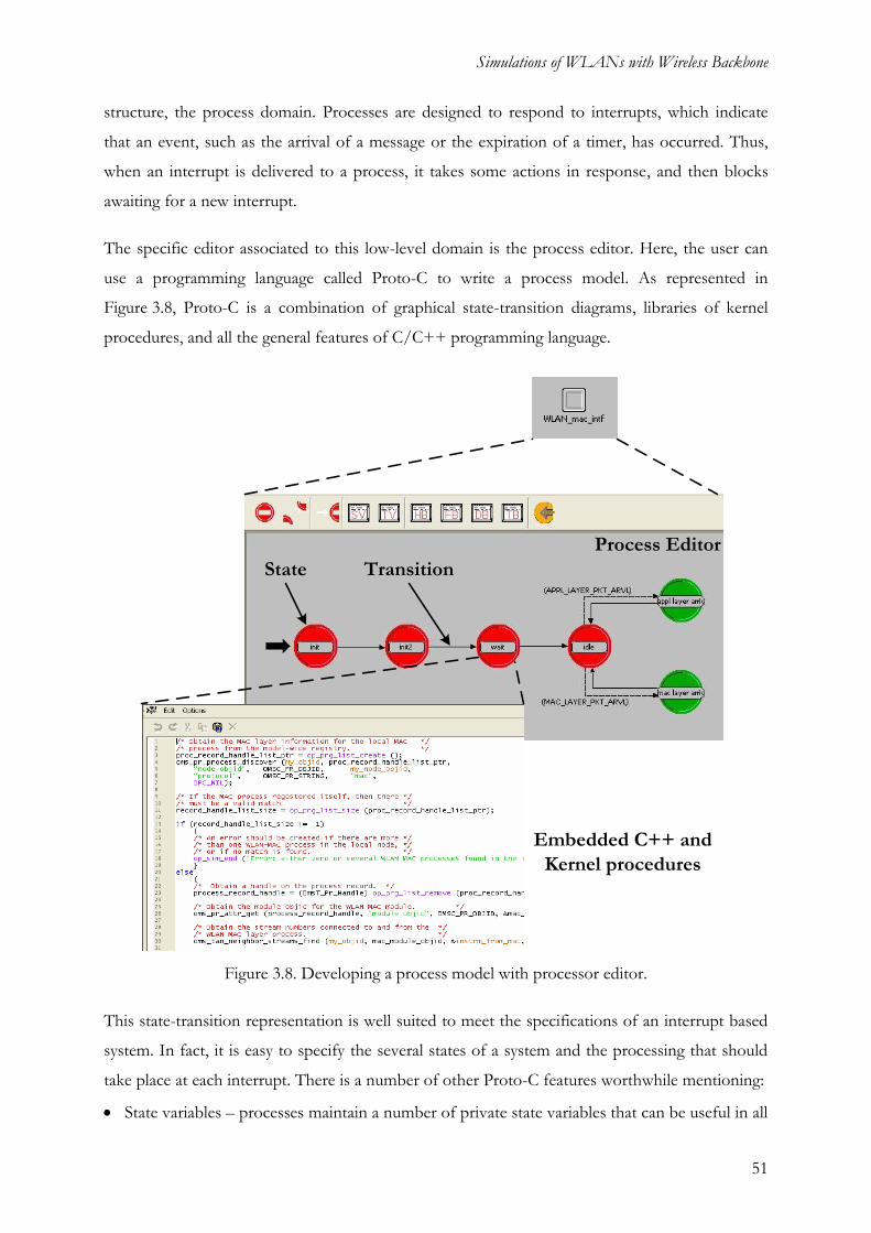
Simulations of WLANs with Wireless Backbone
51
structure, the process domain. Processes are designed to respond to interrupts, which indicate
that an event, such as the arrival of a message or the expiration of a timer, has occurred. Thus,
when an interrupt is delivered to a process, it takes some actions in response, and then blocks
awaiting for a new interrupt.
The specific editor associated to this low-level domain is the process editor. Here, the user can
use a programming language called Proto-C to write a process model. As represented in
Figure 3.8, Proto-C is a combination of graphical state-transition diagrams, libraries of kernel
procedures, and all the general features of C/C++ programming language.
Process Editor
Embedded C++ and
Kernel procedures
State Transition
Figure 3.8. Developing a process model with processor editor.
This state-transition representation is well suited to meet the specifications of an interrupt based
system. In fact, it is easy to specify the several states of a system and the processing that should
take place at each interrupt. There is a number of other Proto-C features worthwhile mentioning:
State variables – processes maintain a number of private state variables that can be useful in all

Performance Evaluation in All-Wireless Wi-Fi Networks
52
the implemented decisions and actions.
State executives – each state can specify the execution of some actions when the process
enters or leaves the state. These actions are programmed by using the flexibility of C++ and
the functionality of kernel procedures within two executives: the Enter and the Exit ones.
Transition conditions – the determination whether a transition between states may occur or
not can be expressed in terms of a C++ condition statement, which may use both properties
of an interrupt and values of the state variables.
Transition executives – resembling state executives, it is possible to specify general actions to
be executed during a transition between states.
The three editors (project, node and process) described previously are the basic components of
the interface environment of Modeler. There are a number of other tools to support the usage of
these model-specification editors where a user can perform several specific tasks. The most
important auxiliary editors are listed in Table 3.1, together with a simple description of their
purpose.
Table 3.1. Modeler secondary editors – incomplete list (adapted from [OPMo06]).
Editor Purpose
Link Model Editor Create, edit, and view link models.
Analysis Configuration Editor
(Analysis Tool)
Plot and process numerical data generated by simulations.
Probe Model Editor Identify sources of statistics and animation that are to be collected during a simulation.
Simulation Sequence Editor
(Simulation Tool)
Design and run sequences of simulations, each potentially configured with different inputs and/or outputs.
Packet Format Editor Specify packet format, defining the order, data type, and size of fields contained within the packet.
PDF Editor Create, edit, and view probability density functions (PDFs)
3.2.3 Discrete Event Simulations
The tools introduced in Subsection 3.2.2 allow the complete definition of a network model, with
a more or less detailed specification of its components. During a simulation run, the progression
of simulation time is decomposed into individual points (events) where the state of the model can

Simulations of WLANs with Wireless Backbone
53
change. This approach has some implications in the interpretation of simulation time, which is
considered simply as a variable maintained by the simulation kernel with no direct relation to the
actual time. Actually, the simulation time can be viewed as a variable that “jumps” from the time
of occurrence of a specific event to the time of the following one. Figure 3.9 gives a schematic
perspective of this concept.
Event
Events can cluster at the
same simulation time
Event densities
are variable
Simulation
Time
Figure 3.9. Typical simulation timeline.
Modeler simulations manage events in an event list. The simulation kernel is responsible for
inserting or deleting events from the list when they are generated or cancelled. The purpose of
maintaining a list of events is to guarantee that they are executed at the correct time order, since
each event has an associated time at which it is specified to occur.
At the beginning of a simulation, the event list receives from the network model components (or
to be more exact from their underlying processes) all the initially scheduled events. Just after the
beginning of the simulation, the header of the list becomes an interrupt, being delivered by the
kernel to the appropriate module. Then, the process that runs within the module gains control of
the simulation and executes all the necessary actions in response to the received interrupt. These
actions can result in the generation of new events, scheduled for any future time, or in the
cancellation of events already inserted in the list. At the end of the processing of the first
interrupt, simulation kernel regains control and deletes the event that was already executed,
allowing the second event to reach the top of the list. The simulation cycle goes on, until there
are no more events to process. It is easy to understand that the event list is dynamic. It may
continually grow or shrink while a simulation runs, following a particular pattern that depends on
the activities that are modelled.
Modeler events are much more than abstract entities representing simulation activities and having
an associated time of execution. In fact, they are relatively complex structures with a number of
attributes describing the way they should be executed. Based on this information, the process

Performance Evaluation in All-Wireless Wi-Fi Networks
54
handling the event decides which action should be taken. Table 3.2 lists some of the most
important event attributes.
Table 3.2. Event attributes summary (adapted from [OPMo06]).
Attribute Name Attribute Meaning
Time Simulation time at which event should be executed.
Execution ID Unique identifier related to event’s order of execution.
Source object ID Object ID of the module that has processed the event during which this event was generated.
Module Module (node domain object) where event will occur.
Process Unique process that will receive the event.
Type Classification of the activity related to the event.
To obtain the attributes of an event, a process model makes use of several kernel procedures
provided as built-in libraries.
3.2.4 Data Collection and Analysis
The main goal of most modelling efforts is to obtain measures of a system’s performance, or to
evaluate its behaviour in some particular aspects. This way, Modeler provides several mechanisms
to collect the desired data from one or more simulation runs of a system model. There are three
basic output types:
Output vectors – vectors can be viewed as a collection of pairs of values from two different
variables, one considered as independent (abscissa) and the other as dependent (ordinate).
Usually, the independent variable of a vector is the simulation time. This output type is very
useful when it is necessary to monitor the evolution of some parameter of interest during the
entire simulation time. Note that it is possible to generalise the concept of vector by storing in
an output multiple ordinate values with the same abscissa value.
Output scalars – scalars are individual values obtained over a single simulation run,
representing a metric of interest. Typically, they are averages, standard deviations, peak values
and so on, obtained from a set of measurements. Frequently, scalar statistics are obtained
from an output vector collected during a simulation. In fact, from a single output vector, it is
possible to obtain several scalars. A scalar output resulting from just one simulation run can
be of limited interest. However, Modeler allows the configuration of several simulations

Simulations of WLANs with Wireless Backbone
55
running automatically one after the other, with different values for some parameter of interest
characterising the system model under analysis. Scalars obtained from each simulation run can
be combined in a single graphic, allowing the observation of how a system variable varies as a
function of another system parameter.
Animations – In contrast to previous output types, animations are not numerical statistics.
They are dynamic graphical representations of selected events that occurred during a
simulation. Modeler provides several predefined animations, as for instance: packet flow, node
movement and state transitions.
Besides these basic output types, a user can use the general programmability of models to define
a set of custom outputs to collect data during a simulation.
Before running a simulation, a user must select which parameters he/she wants to monitor from
the vast number of possible statistics. This selection is performed by specifying a list of probes,
which indicates that some particular scalar statistics, vector statistics and forms of animations
should be collected. Probes are selected at network domain level, using the Choose Results
operation in the project editor. Figure 3.10 shows the probes that are available at network level
for WLAN models.
Figure 3.10. Aspect of a Choose Results window (accessible from project editor).
In addition, other advanced forms of probes can be specified in the probe editor (refer to
Table 3.1).
To analyse and visualise data collected in the various types of outputs, it is possible to use all the
basic access mechanisms provided by the project editor. A more complete investigation can be

Performance Evaluation in All-Wireless Wi-Fi Networks
56
accomplished using the analysis tool (see Table 3.1), which is a complete graphical and numerical
processing environment.
Output vectors, as well as scalars, resulting from multi-simulation studies can be loaded and
displayed as traces. As an example, Figure 3.11 is the visualisation of a vector collected during a
simulation run. The trace represented in the figure shows the evolution of FTP traffic sent during
simulation time.
Figure 3.11. Example of a vector data analysis panel.
Figure 3.12 shows an example of a trace obtained from a multi-simulation scalar output. Here,
network load was continuously modified over several simulations to evaluate the behaviour of
end to end delay.
Figure 3.12. Example of a scalar data analysis panel.

Simulations of WLANs with Wireless Backbone
57
3.2.5 WLAN Models
OPNET Modeler comes with a complete suite of WLAN models shipped as part of the standard
model library. Release 12.0 together with the Wireless Module implements the features of
IEEE 802.11, 802.11a, 802.11b, 802.11g and 802.11e standards. Some of these features are
highlighted below:
Access mechanism – both DCF and PCF are supported.
Frame exchange sequence – reliable data transmission is supported via threshold-based RTS-
CTS exchange.
Fragmentation and reassembly – fragmentation is available, based on the size of data packets
received from higher layers. The several fragments are reassembled at the destination station.
Inter-operability support – it is possible to model WLANs where capable and non-capable
11b, 11g and 11e nodes coexist.
Physical layer technologies – FHSS, IR, DSSS, OFDM and ERP-OFDM. Note that,
optionally, it is possible to auto-assign channels to a BSS.
Supported data rates – 1, 2, 5.5, 6, 9, 11, 12, 18, 24, 36, 48 and 54 Mbps.
Supported modulations – DPSK, BPSK, QPSK, CCK-55, CCK-11, QAM-16 and QAM-64.
Communication distance – the maximum communication distance between two WLAN
nodes is modelled as a function of three parameters: transmission power of the source node,
path-loss propagation model, and receiver sensitivity.
The WLAN model suite is composed of several node and process models that can be combined
to form a network model. The remaining of this section is dedicated to describe some of the
most important models that are needed to implement a WLAN.
Figure 3.13 and Figure 3.14 depict the internal structure of two node models, wlan_wkstn and
wlan_station respectively, that can be used both as a wireless station and as an AP. While the
former implements all layers from the physical to the application one, the latter just implements
the 802.11 protocol. Higher layers are emulated by a bursty source and a sink module.
All MAC layer functionalities are executed in the wireless_lan_mac module, whose behaviour is
controlled by the wlan_dispacth process. It has a very simple structure, with just one state, and can
be viewed as the parent process for the WLAN functionality. Depending on whether, or not,
standard 802.11e is enabled on the node, wlan_dispacth spawns one of two possible child
processes: wlan_mac_hacf if 802.11e is enabled or wlan_mac otherwise. The interface between MAC

Performance Evaluation in All-Wireless Wi-Fi Networks
58
and higher layers is performed by the ARP (Address Resolution Protocol) module, or by its
equivalent wlan_mac_intf.
Physical
Layer
MAC
Layer
Network
Layer
Application
and Transport
Layers
Figure 3.13. Internal structure of wlan_wkstn node model.
Figure 3.14. Internal structure of wlan_station node model.
As described in Section 3.1, in several scenarios, there is the need to use a node model with two
wireless interfaces: one for the access network and another for the backbone one. Modeler
provides a model complying with these needs, the wlan2_router node model that is depicted in
Figure 3.15. When this node is configured as an AP, which is the default configuration, it can
connect a BSS with a wireless DS.
In order to evaluate the performance of a WLAN, several statistics can be collected while
running a simulation. They can be obtained at a global, per-node, or per-module basis. All the

Simulations of WLANs with Wireless Backbone
59
available probes at node and module levels are listed in Figure 3.16. Note that all the evaluation
metrics defined in Section 3.1.2 are already implemented (highlighted in the figure).
Routing Domain
Node Management
Wireless
Interfaces
Figure 3.15. Internal structure of wlan2_router node model.
WLAN Node Statistics
WLAN Module Statistics
(wireless_lan_mac)
Figure 3.16. WLAN Node and Module statistics.
When deploying a wireless network, as for instance a WLAN, OPNET uses the concept of radio

Performance Evaluation in All-Wireless Wi-Fi Networks
60
links to establish a connection between any radio transmitter-receiver. Radio links are not
represented by objects, rather existing as a function of dynamic conditions, such as frequency
band, modulation type, transmitter power, distance, and antenna pattern. Thus, radio transmitter
and receiver objects are responsible for determining when and if a packet is successfully received.
One of the performed calculations is the propagation loss between transmitter and receiver,
which, by default, is assumed to be the well-known free-space model. More details on the
implementation of radio links can be found in [OPMo06].
3.3 WLANs with Wireless Backbone using OPNET
By using OPNET Modeler tools and models, it is possible to implement the scenario described
in Subsection 3.1.2, providing all the necessary degrees of freedom. Figure 3.17 shows the
implementation model at the network level.
Figure 3.17. Implementation model using OPNET Modeler.
The network represented in Figure 3.17 is composed of several nodes (objects), which are

Simulations of WLANs with Wireless Backbone
61
instances of node models picked from the WLAN model suite. The used node models are:
Application Config, Profile Config, wlan_wkstn, wlan_server and wlan2_router. In order to describe the
implementation scenario, the paragraphs below give a generic description of each model,
describing their role in the network.
The Application Config model, which describes the behaviour of node Applications, is used to
configure all the applications running in client stations. It provides a set of preconfigured models
of the following commonly used network applications: FTP, E-mail, Remote Login, Database,
HTTP (Hyper Text Transfer Protocol), Print, Voice and Voice Conferencing. Each of these
models has specific attributes that can be configured to generate and appropriate traffic pattern.
Applications defined in the Applications node are used by the Profiles node, which is an instance
of the Profile Config model, to create user profiles. These user profiles can be assigned to different
nodes in the network, defining the usage pattern of the applications that are running in the node.
From the previous discussion, it is easy to understand that the network traffic load is defined by a
three steps procedure:
First, the Applications node is used to configure all applications that can run in the network.
Secondly, based on the applications defined in the first step, the Profiles node is used to
define user profiles. Each profile must specify when, how long, and how often each
application is used.
Finally, the defined profiles are assigned to client stations.
It is important to note that Applications and Profiles objects are not like client stations or servers
– they do not represent a physical entity of the network. Their goal is to help on the task of
traffic generation.
All client stations (Stat1 to StatN) associated with MAP1 are instances of the wlan_wkstn model,
representing a workstation with client-server and client-client applications running over TCP/IP
and UDP/IP. There are also three instances of wlan_wkstn at the servers side (associated with
MAP2) dedicated to the client-client applications running over the network. The remaining nodes
associated with MAP2 are instances of the wlan_servers model that can be configured to act as
servers for the client stations applications.
Finally, MAP1 and MAP2 nodes are the focal points of the network. They act as MAPs,
participating in the backbone network (BSS0), and in access networks BSS1 and BSS2,
respectively. Thus, most part of evaluation metrics are collected within these nodes, as already

Performance Evaluation in All-Wireless Wi-Fi Networks
62
described in Subsection 3.1.2. MAP1 and MAP2 are instances of wlan2_router (Figure 3.15), which
models a wireless router with two RIs.
When having client stations and servers in different BSSs, all the generated traffic has to pass
through BSS0 using the IP routing protocols implemented in the wlan2_router model. Several IP
routing protocols are provided by OPNET Modeler, with the function of helping in the task of
moving datagrams from source to destination addresses. One important function of such
protocols is to maintain information about the proper routes to use for each possible destination
node, which implies the sharing of information among routers during network setup and while it
evolves.
Although the choice on which routing protocol to use is an in-depth topic in network design, this
is not the aim of the present study. This way, and since all nodes in the implementation network
are fixed, the option is to define static routing tables in MAP1 and MAP2, in order to reduce the
traffic delivered to the network related to routing protocols. To do this, first it is necessary to
assign an IP address to each RI in the network, and then, to configure the attribute IP > IP
Routing Parameters > Static Routing Table of both MAP1 and MAP2, Figure 3.18.
Figure 3.18. Static Routing Table attribute.
To finalise this introduction to the implementation scenario, Table 3.3, Table 3.4 and Table 3.5
provide a short description of the network nodes main attributes, instances of wlan_wkstn,
wlan_server and wlan2_router.
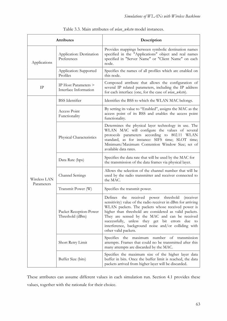
Simulations of WLANs with Wireless Backbone
63
Table 3.3. Main attributes of wlan_wkstn model instances.
Attributes Description
Applications
Application: Destination Preferences
Provides mappings between symbolic destination names specified in the "Applications" object and real names specified in "Server Name" or "Client Name" on each node.
Application: Supported Profiles
Specifies the names of all profiles which are enabled on this node.
IP IP Host Parameters > Interface Information
Composed attribute that allows the configuration of several IP related parameters, including the IP address for each interface (one, for the case of wlan_wkstn).
Wireless LAN Parameters
BSS Identifier Identifies the BSS to which the WLAN MAC belongs.
Access Point Functionality
By setting its value to “Enabled”, assigns the MAC as the access point of its BSS and enables the access point functionality.
Physical Characteristics
Determines the physical layer technology in use. The WLAN MAC will configure the values of several protocols parameters according to 802.11 WLAN standard, as for instance: SIFS time; SLOT time; Minimum/Maximum Contention Window Size; set of available data rates.
Data Rate (bps) Specifies the data rate that will be used by the MAC for the transmission of the data frames via physical layer.
Channel Settings Allows the selection of the channel number that will be used by the radio transmitter and receiver connected to the MAC.
Transmit Power (W) Specifies the transmit power.
Packet Reception-Power Threshold (dBm)
Defines the received power threshold (receiver sensitivity) value of the radio receiver in dBm for arriving WLAN packets. The packets whose received power is higher than threshold are considered as valid packets. They are sensed by the MAC and can be received successfully, unless they get bit errors due to interference, background noise and/or colliding with other valid packets.
Short Retry Limit Specifies the maximum number of transmission attempts. Frames that could no be transmitted after this many attempts are discarded by the MAC.
Buffer Size (bits) Specifies the maximum size of the higher layer data buffer in bits. Once the buffer limit is reached, the data packets arrived from higher layer will be discarded.
These attributes can assume different values in each simulation run. Section 4.1 provides these
values, together with the rationale for their choice.

Performance Evaluation in All-Wireless Wi-Fi Networks
64
Table 3.4. Main attributes of instances of wlan_server model.
Attributes Description
Applications Application: Supported Services
Parameters to start and setup services for various applications at the server. Clients can send traffic to the server for only those applications which are supported by this attribute (one, for the case of wlan_server).
IP IP Host Parameters > Interface Information
Composed attribute that allows the configuration of several IP related parameters, including the IP address for each interface.
Wireless LAN Parameters The same as Table 3.3.
Table 3.5. Main attributes of instances of wlan2_router model.
Attributes Description
IP Routing Parameters
Interface Information Composed attribute that allows the configuration of several IP related parameters, including the IP address for each interface (two, for the case of wlan2_router).
Static Routing Table Allows the configuration of a user defined static routing table.
Wireless LAN Parameters The same as Table 3.3. However, since wlan2_router has two RIs, there are two identical sets of Wireless LAN Parameters: one for interface 0 and other for interface 1.

Results Analysis
65
Chapter 4
Results Analysis
4 Results Analysis
Using the concepts introduced in previous chapters, this chapter starts by defining all Simulation
Sets analysed during the present study, together with an analysis of results statistical meaning. A
detailed results analysis is then conducted, pointing out the most important observations for each
set of simulations.

Performance Evaluation in All-Wireless Wi-Fi Networks
66
4.1 Simulations Setup
In order to analyse the impact of the degrees of freedom variation on network performance in a
systematic manner, it is necessary to establish several Simulation Sets. Each Simulation Set is
composed of several Simulations, representing a specific realisation of the varying degrees of
freedom. As mentioned before, in each Simulation Sets there are always two varying degrees of
freedom, one being the Technology used in BSS0. The values that this parameter can assume,
together with the related settings for access networks (BSS1 and BSS2), are represented in Table
4.1, defining four simulation scenarios. Note that these parameters are configured in the Wireless
LAN Parameters attribute of each node.
Table 4.1. Technology used in each BSS.
Parameters
Scenario Designation
(values for Technology used in BSS0)
Back11b_SameCh Back11b_DiffCh Back11a Back11g
Standard in BSS0(1) 802.11b 802.11b 802.11a 802.11g
Channel in BSS0(1) Channel 6
(2.426 MHz)
Channel 1
(2.401 MHz)
5 GHz Channel 36
(5.170 MHz)
Channel 6
(2.426 MHz)
Standard in BSS1 802.11b 802.11b 802.11b 802.11b
Channel in BSS1 Channel 6
(2.426 MHz)
Channel 6
(2.426 MHz)
Channel 1
(2.401 MHz)
Channel 1
(2.401 MHz)
Standard in BSS2 802.11b 802.11b 802.11b 802.11b
Channel in BSS2 Channel 6
(2.426 MHz)
Channel 11
(2.451 MHz)
Channel 11
(2.451 MHz)
Channel 11
(2.451 MHz)
(1) These two parameters represent the degree of freedom Technology used in BSS0.
Scenario Back11b_SameCh represents the worst solution, with the use of the same 802.11
standard and the same radio channel in every BSS. It is used as a basis for comparison of the
performance of the other three scenarios, in order to evaluate which of the available technologies
(802.11a, b and g) best fit the requirements of a wireless backbone. The results obtained from
simulating these four scenarios are used to answer to the first open issue listed in Subsection
3.1.2.
Using the scenarios defined in Table 4.1, each Simulation Set can be viewed as a sequence of
simulation runs for each scenario, which last until the second degree of freedom assumes all its
possible values. Since the factor that differentiates each Simulation Set is the second varying

Results Analysis
67
degree of freedom, five Sets are defined: Service Mix, Distance – MAPs, Number of Clients,
Data Rate, and Buffer Size, having a direct relation to the open issues referred in Subsection
3.1.2, which are the guidelines of the present study.
Before the description of each Simulation Set, it is important to carry out some considerations on
the definition of profiles and applications used in the network. As mentioned in Section 3.3, this
definition is fundamental to characterise the traffic load delivered to the network. Although
several applications can be present in a profile, the option was to configure just one application
per profile, which, as described later, is useful in the task of services mix definition. This way, six
different profiles were configured with the attributes provided in Table 4.2.
Table 4.2. Profiles definition.
Attributes Profiles
Profile_0 Profile_1 Profile_2 Profile_3 Profile_4 Profile_5
Start Time [s] uniform (60,120)
Duration Until End of Simulation
Ap
plic
atio
ns
Name E-mail FTP Video
Conferencing Video
Streaming VoIP
Web Browsing
Start Time Offset [s]
No Offset No Offset No Offset No Offset No Offset No Offset
Duration [s] End of Profile
End of Profile
uniform (100, 140)
uniform (100, 600)
uniform (100, 140)
End of Profile
Repeatability > Inter-rep. Time [s]
Not Applicable
Not Applicable
exp (900) exp (900) exp (600) Not
Applicable
In order to clarify the meaning of Profiles attributes, Figure 4.1 provides a graphical
representation of Profile_1 and Profile_4 time related attributes. Settings of the applications
attributes referred in Table 4.2 are specified in Annex A. A detailed description of each attribute
is also provided.
After having an adequate set of profiles, it is possible to define the values that the AD parameter
can assume. Basically, AD values, which are characterised in Table 4.3, represent several
distributions of profiles assigned to client stations. The value ReferSM (Reference Service Mix) is
adapted from the applications distribution provided in [LjDa06] and [Karl04], for business users.
It is considered as the basic value for the AD parameter, and provides the most balanced
distribution between applications with and without real time requirements. RTiCeSM (Real Time
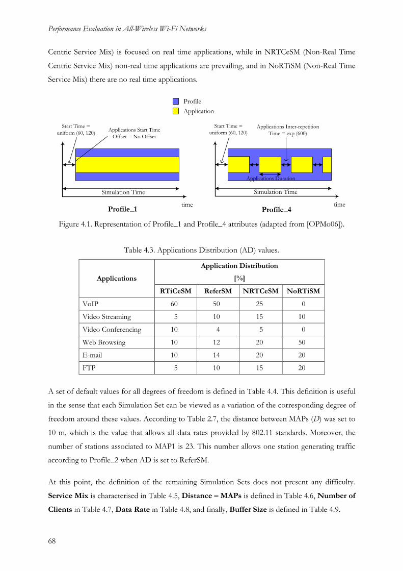
Performance Evaluation in All-Wireless Wi-Fi Networks
68
Centric Service Mix) is focused on real time applications, while in NRTCeSM (Non-Real Time
Centric Service Mix) non-real time applications are prevailing, and in NoRTiSM (Non-Real Time
Service Mix) there are no real time applications.
time
Start Time =
uniform (60, 120)Applications Start Time
Offset = No Offset
Simulation Time
time
Start Time =
uniform (60, 120)Applications Inter-repetition
Time = exp (600)
Simulation Time
Applications Duration
Profile
Application
Profile_1 Profile_4
Figure 4.1. Representation of Profile_1 and Profile_4 attributes (adapted from [OPMo06]).
Table 4.3. Applications Distribution (AD) values.
Applications
Application Distribution
[%]
RTiCeSM ReferSM NRTCeSM NoRTiSM
VoIP 60 50 25 0
Video Streaming 5 10 15 10
Video Conferencing 10 4 5 0
Web Browsing 10 12 20 50
E-mail 10 14 20 20
FTP 5 10 15 20
A set of default values for all degrees of freedom is defined in Table 4.4. This definition is useful
in the sense that each Simulation Set can be viewed as a variation of the corresponding degree of
freedom around these values. According to Table 2.7, the distance between MAPs (D) was set to
10 m, which is the value that allows all data rates provided by 802.11 standards. Moreover, the
number of stations associated to MAP1 is 23. This number allows one station generating traffic
according to Profile_2 when AD is set to ReferSM.
At this point, the definition of the remaining Simulation Sets does not present any difficulty.
Service Mix is characterised in Table 4.5, Distance – MAPs is defined in Table 4.6, Number of
Clients in Table 4.7, Data Rate in Table 4.8, and finally, Buffer Size is defined in Table 4.9.

Results Analysis
69
Table 4.4. Implementation Model – default settings.
Degree of Freedom Value
AD ReferSM
D [m] 10
N 23
RN in BSS0 [Mbps] 11
Bf [kbit] 1024
Table 4.5. Service Mix Simulation Set definition.
Degree of Freedom Simulation #
1 2 3 4
AD RTiCeSM ReferSM NRTCeSM NoRTiSM
D [m]
Default Settings N
RN in BSS0 [Mbps]
Bf [kbit]
Table 4.6. Distance – MAPs Simulation Set definition.
Degree of Freedom
Simulation #
2 5 6 7 8 9 10 11 12 13
D [m] 10 20 30 40 60 80 120 160 220 280
AD
Default Settings N
RN in BSS0 [Mbps]
Bf [kbit]
The correspondence between the respective degree of freedom, for each of the previous
Simulation Sets, and a specific network/node attribute is given below:
AD is defined by using attributes “Applications > Application: Destination Preferences” and
“Applications > Application: Supported Profiles” of all client stations.
D, which represents the physical distance between MAPs, is defined at model setup, during
the deployment of MAP1 and MAP2 in the network.
N is also defined at model setup. Client stations are randomly deployed around MAP1 using
the rapid configuration tool provided with OPNET Modeler (for more details refer to
Modeler documentation [OPMo06]).

Performance Evaluation in All-Wireless Wi-Fi Networks
70
RN in BSS0 is configured using the “Wireless LAN Parameters > Data Rate” attribute of both
MAP1 and MAP2.
Bf is configured using the “Wireless LAN Parameters > Buffer Size” attribute.
Table 4.7. Number of Clients Simulation Set definition.
Degree of Freedom
Simulation #
14 2 15 16
N 10 23 30 40
AD
Default Settings D [m]
RN in BSS0 [Mbps]
Bf [kbit]
Table 4.8. Data Rate Simulation Set definition.
Degree of Freedom Simulation #
17 18 2
RN in BSS0 [Mbps] 1 5.5 11
AD
Default Settings D [m]
N
Bf [kbit]
Table 4.9. Buffer Size Simulation Set definition.
Degree of Freedom Simulation #
19 20 2
Bf [kbit] 64 256 1024
AD
Default Settings D [m]
N
RN in BSS0 [Mbps]
From the Wireless LAN Parameters attributes described in Section 3.3, there is still a few that
need to be defined. The values of these attributes are presented in Table 4.10, being the same for
all network interfaces and in every simulation runs.

Results Analysis
71
Table 4.10. Common Wireless LAN Parameters attributes.
Attributes Value
Transmit Power [W] 0.005
Packet Reception-Power Threshold [dBm]
-95
Short Retry Limit 7
All Simulations presented in Table 4.4 to Table 4.9 consist of at least 4 simulation runs, one for
each scenario: Back11b_SameCh, Back11b_DiffCh, Back11a and Back11g. In order to provide
statistical meaning to results, 10 simulation runs were performed for each scenario, leading to a
total of 40 runs for the complete Simulation. To give an example, for the Service Mix Simulation
Set, 160 simulation runs were conducted (160 = 4 (scenarios, representing the values for
Technology used in BSS0 degree of freedom) × 10 × 4 (Simulations)).
The number of 10 simulation runs per scenario was obtained from a study of the results provided
by two sequences of simulations. The goal of this study was to assess the number of simulation
runs that need to be performed, until the variation of the cumulative mean becomes stable. The
scenario used during the study was Back11b_DiffCh, configured with the implementation model
default settings (Table 4.4). The considered evaluation metric was R in MAP2, which measures
the traffic flowing from clients to servers.
This scenario was simulated over two sequences of 25 simulation runs, using two distinct sets of
25 Seeds. Note that a Seed is a parameter of a simulation run configuration, acting as the initial
value for all random number generators used during a discrete event simulation. This way, the
use of different Seeds leads to different results.
To analyse the cumulative mean of a given evaluation metric X after several simulation runs, it is
useful to define a measure of stability, Δ:
_ _
_% 100
cum s cum S
cum S
X X
X
(4.1)
where,
s is the simulation run index.
S is the total number of simulation runs conducted during the study of stability.

Performance Evaluation in All-Wireless Wi-Fi Networks
72
Xcum_s is the X cumulative mean at simulation run s.
Xcum_S is the final X cumulative mean (mean of the means from all simulation runs).
The cumulative mean of X at simulation run s is given by:
_
_ 1
smean i
cum s i
XX
s
(4.2)
where,
Xmean_i is the mean of X for simulation run i.
Additionally it is also useful to define the cumulative maximum of an evaluation metric X:
1
smax_ i
MAX _ s i
XX
s
(4.3)
where,
Xmax_i is the maximum value of X obtained during simulation run i.
As already mentioned, Back11b_SameCh is the worst case scenario that is used in subsequent
sections as a reference to assess the performance increase of other scenarios. To quantify this
assessment in terms of throughput, it is convenient to define a relative gain to Back11b_SameCh,
(4.4). GR is a function of x (Technology used in BSS0) and y (any of the other degrees of
freedom).
10
10 11
MAX _
R MAX _
R x, yG x, y
R Back b _ SameCh, y (4.4)
The values of Δ for the two sets of 25 seeds, and using R in BSS2 as the evaluation metric, are
given at Figure 4.2. In this figure, it is possible to observe that for s ≥ 10, the values of Δ are less
than 2 %. Thus, it is possible to conclude that running S = 10 simulations per scenario is enough
to obtain results with a reasonable statistical meaning.
This conclusion represents the bottom line of the stability study, which is: all the values presented
in subsequent sections represent the related evaluation metric cumulative mean after 10
simulation runs.

Results Analysis
73
0
5
10
15
20
25
1 2 3 4 5 6 7 8 9 10 11 12 13 14 15 16 17 18 19 20 21 22 23 24 25
s
Δ [
%] Set_1
Set_2
2%
Figure 4.2. Δ for two sets of 25 Seeds (with X = R in BSS2).
Each simulation run intends to simulate the network behaviour during 1 hour, collecting all the
adequate results during this period of time. For instance, Rmean_s represents the Throughput mean
of the entire set of values collected during 1 hour. However, there is a “transitory” period at the
beginning of a simulation run that needs to be ignored, since it can have a misleading effect in
evaluation metric means. To select the time period to discard, Figure 4.3 shows the value of
Global Delay over 1 hour of simulation, using the same implementation model settings as the
stability study (with one set of 25 Seeds). Global Delay represents the end-to-end delay of all the
packets received by wireless LAN MACs of all WLAN nodes in the network and forwarded to
the higher layer.
Time
Glo
ba
l D
ela
y [s]
Figure 4.3. Global Delay for 25 simulation runs.
From the results presented in Figure 4.3, it is possible to conclude that the first 5 minutes of the

Performance Evaluation in All-Wireless Wi-Fi Networks
74
simulation must be discarded. This way, parameter Duration of the simulation configuration was
set to 65 minutes.
Since OPNET Modeler is a discrete event simulator, the actual time that takes to complete a
simulation is less than 65 minutes. Table 4.11 represents the simulation times for every
Simulation defined in Table 4.4 to Table 4.9. When analysing the table, remember that each
Simulation # consists of 40 simulation runs.
Table 4.11. Actual simulation times.
Simulation # Simulation time Simulation # Simulation time
1 13h 30m 43s 11 12h 10m 54s
2 12h 29m 04s 12 11h 55m 06s
3 08h 15m 20s 13 11h 53m 38s
4 03h 03m 44s 14 03h 56m 27s
5 12h 30m 00s 15 17h 29m 01s
6 11h 47m 26s 16 26h 13m 59s
7 11h 50m 19 17 08h 31m 33s
8 12h 11m 55s 18 12h 17m 22s
9 11h 55m 54s 19 12h 33m 37s
10 11h 47m 48s 20 12h 31m 25s
The sum of all values presented in Table 4.11 is 238h 55m 15s (approximately 12 consecutive
days), not including the time spent during initial studies (cumulative mean stability and
“transitory” period). This value shows that, due to the large amount of events to be handled,
simulations of the implementation model are a very time consuming task.
4.2 Service Mix
The goal of defining the Service Mix Simulation Set is to assess the impact of having different
traffic patterns coming from the clients’ side on the performance of applications and backbone
network. The two varying degrees of freedom are Technology used in BSS0 and AD, assuming
all their possible values as defined in Section 4.1:
Technology used in BSS0 = Back11b_SameCh; Back11b_DiffCh; Back11a; Back11g.
AD = RTiCeSM; ReferSM; NRTCeSM; NoRTiSM.
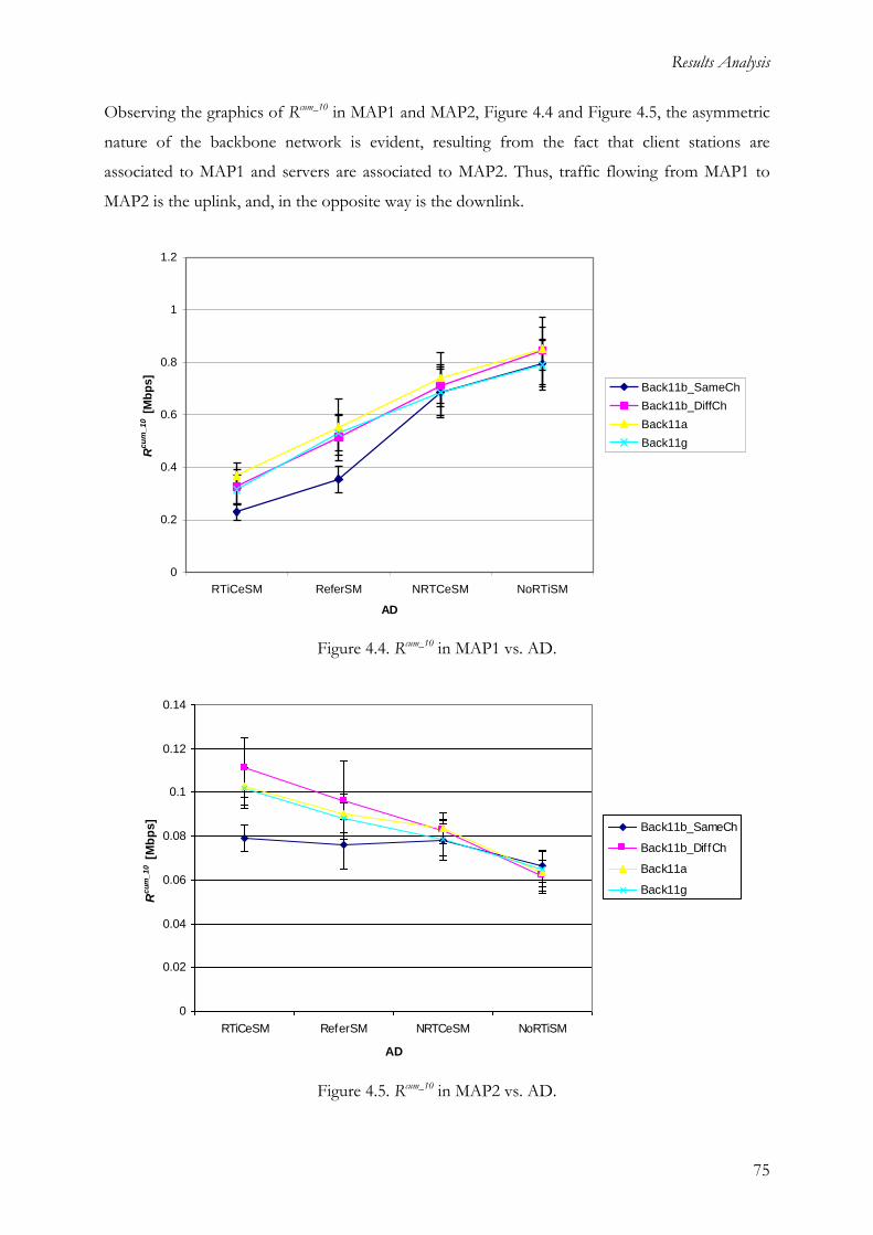
Results Analysis
75
Observing the graphics of Rcum_10 in MAP1 and MAP2, Figure 4.4 and Figure 4.5, the asymmetric
nature of the backbone network is evident, resulting from the fact that client stations are
associated to MAP1 and servers are associated to MAP2. Thus, traffic flowing from MAP1 to
MAP2 is the uplink, and, in the opposite way is the downlink.
0
0.2
0.4
0.6
0.8
1
1.2
RTiCeSM ReferSM NRTCeSM NoRTiSM
AD
Rcu
m_10 [
Mb
ps]
Back11b_SameCh
Back11b_DiffCh
Back11a
Back11g
Figure 4.4. Rcum_10 in MAP1 vs. AD.
0
0.02
0.04
0.06
0.08
0.1
0.12
0.14
RTiCeSM ReferSM NRTCeSM NoRTiSM
AD
Rc
um
_1
0 [
Mb
ps]
Back11b_SameCh
Back11b_DiffCh
Back11a
Back11g
Figure 4.5. Rcum_10 in MAP2 vs. AD.
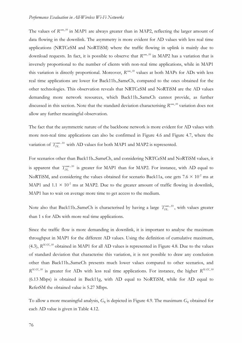
Performance Evaluation in All-Wireless Wi-Fi Networks
76
The values of Rcum_10 in MAP1 are always greater than in MAP2, reflecting the larger amount of
data flowing in the downlink. The asymmetry is more evident for AD values with less real time
applications (NRTCeSM and NoRTiSM) where the traffic flowing in uplink is mainly due to
download requests. In fact, it is possible to observe that Rcum_10 in MAP2 has a variation that is
inversely proportional to the number of clients with non-real time applications, while in MAP1
this variation is directly proportional. Moreover, Rcum_10 values at both MAPs for ADs with less
real time applications are lower for Back11b_SameCh, compared to the ones obtained for the
other technologies. This observation reveals that NRTCeSM and NoRTiSM are the AD values
demanding more network resources, which Back11b_SameCh cannot provide, as further
discussed in this section. Note that the standard deviation characterising Rcum_10 variation does not
allow any further meaningful observation.
The fact that the asymmetric nature of the backbone network is more evident for AD values with
more non-real time applications can also be confirmed in Figure 4.6 and Figure 4.7, where the
variation of _10cum
DLT with AD values for both MAP1 and MAP2 is represented.
For scenarios other than Back11b_SameCh, and considering NRTCeSM and NoRTiSM values, it
is apparent that _10cum
DLT is greater for MAP1 than for MAP2. For instance, with AD equal to
NoRTiSM, and considering the values obtained for scenario Back11a, one gets 7.6 × 10⁻² ms at
MAP1 and 1.1 × 10⁻² ms at MAP2. Due to the greater amount of traffic flowing in downlink,
MAP1 has to wait on average more time to get access to the medium.
Note also that Back11b_SameCh is characterised by having a large _10cum
DLT , with values greater
than 1 s for ADs with more real time applications.
Since the traffic flow is more demanding in downlink, it is important to analyse the maximum
throughput in MAP1 for the different AD values. Using the definition of cumulative maximum,
(4.3), RMAX_10 obtained in MAP1 for all AD values is represented in Figure 4.8. Due to the values
of standard deviation that characterise this variation, it is not possible to draw any conclusion
other than Back11b_SameCh presents much lower values compared to other scenarios, and
RMAX_10 is greater for ADs with less real time applications. For instance, the higher RMAX_10
(6.13 Mbps) is obtained in Back11g, with AD equal to NoRTiSM, while for AD equal to
ReferSM the obtained value is 5.27 Mbps.
To allow a more meaningful analysis, GR is depicted in Figure 4.9. The maximum GR obtained for
each AD value is given in Table 4.12.
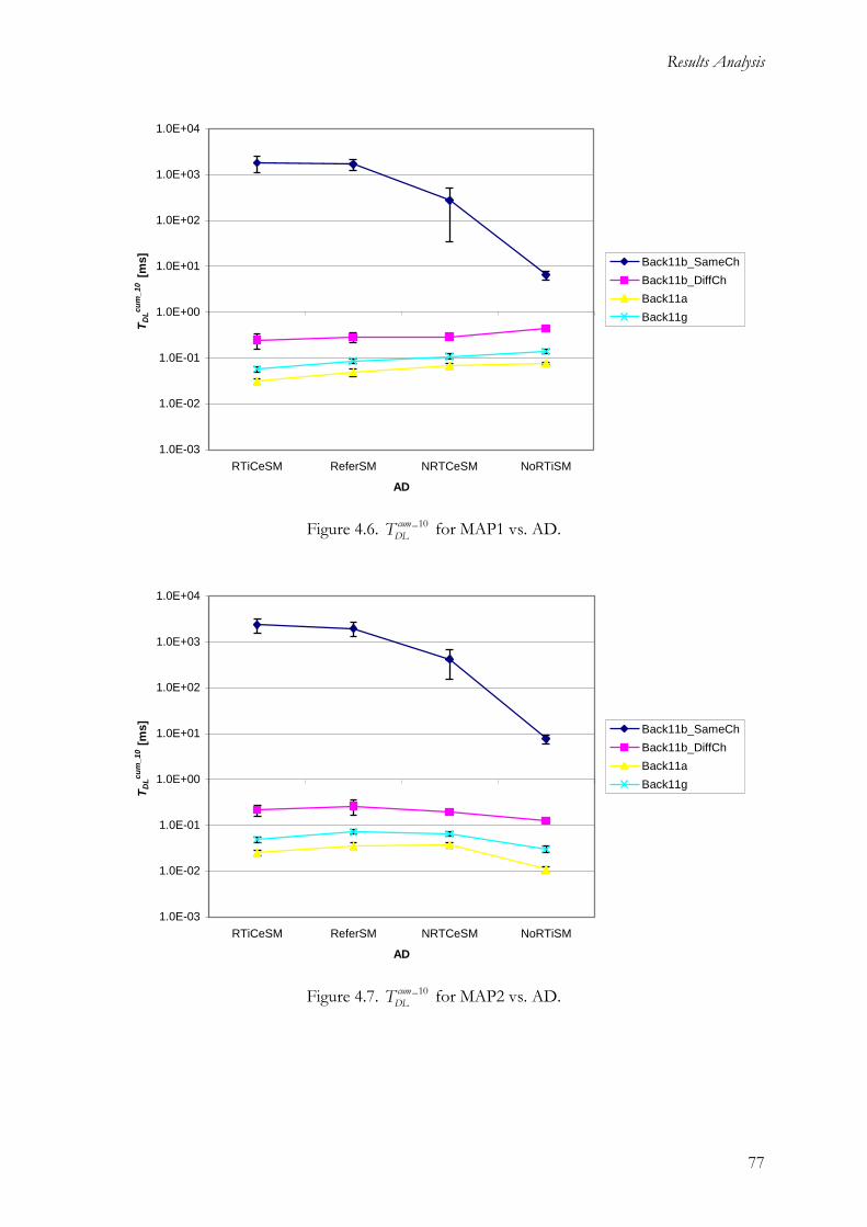
Results Analysis
77
1.0E-03
1.0E-02
1.0E-01
1.0E+00
1.0E+01
1.0E+02
1.0E+03
1.0E+04
RTiCeSM ReferSM NRTCeSM NoRTiSM
AD
TD
Lcu
m_10 [
ms]
Back11b_SameCh
Back11b_DiffCh
Back11a
Back11g
Figure 4.6. _10cum
DLT for MAP1 vs. AD.
1.0E-03
1.0E-02
1.0E-01
1.0E+00
1.0E+01
1.0E+02
1.0E+03
1.0E+04
RTiCeSM ReferSM NRTCeSM NoRTiSM
AD
TD
Lcu
m_10
[ms]
Back11b_SameCh
Back11b_DiffCh
Back11a
Back11g
Figure 4.7. _10cum
DLT for MAP2 vs. AD.
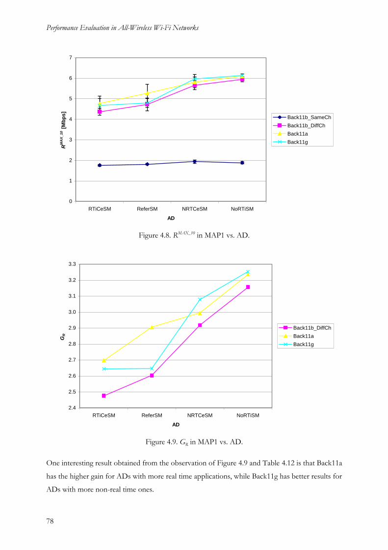
Performance Evaluation in All-Wireless Wi-Fi Networks
78
0
1
2
3
4
5
6
7
RTiCeSM ReferSM NRTCeSM NoRTiSM
AD
RM
AX
_1
0 [
Mb
ps
]
Back11b_SameCh
Back11b_DiffCh
Back11a
Back11g
Figure 4.8. RMAX_10 in MAP1 vs. AD.
2.4
2.5
2.6
2.7
2.8
2.9
3.0
3.1
3.2
3.3
RTiCeSM ReferSM NRTCeSM NoRTiSM
AD
GR
Back11b_DiffCh
Back11a
Back11g
Figure 4.9. GR in MAP1 vs. AD.
One interesting result obtained from the observation of Figure 4.9 and Table 4.12 is that Back11a
has the higher gain for ADs with more real time applications, while Back11g has better results for
ADs with more non-real time ones.

Results Analysis
79
Table 4.12. Maximum values of GR.
x y Maximum GR
Back11a RTiCeSM 2.70
Back11a ReferSM 2.90
Back11g NRTCeSM 3.08
Back11g NoRTiSM 3.25
Considering the previous results, it is clear that the service mix offered by clients to the network
is an important parameter, when deciding which technology to use in the backbone network.
Results show that a distinction can be made between ADs with more (RTiCeSM and ReferSM)
and less (NRTCeSM and NoRTiSM) real time applications. Thus, it is interesting to have an easy
way to obtain evaluation metrics to assess which of these broadest services mixes is present at the
clients’ side. As shown in Figure 4.10, packets size received in a MAP RI2, Prcvd, satisfies this
objective.
0
500
1000
1500
2000
2500
Back11b_SameCh Back11b_DiffCh Back11a Back11g
Technology used in BSS0
Prc
vd
[b
yte
s]
RTiCeSM
ReferSM
NRTCeSM
NoRTiSM
750
Non-Real Time
Real Time
Figure 4.10. Prcvd in MAP1 vs. Technology used in BSS0.
Prcvd is not directly available from the WLAN model statistics suite. It is calculated using the
statistics Data Traffic Rcvd (bps) and Data Traffic Rcvd (packet/s), giving the average size of all
data packets received in RI2. From the obtained results, it is possible to consider that if
Prcvd > 750 bytes, clients’ service mix is real time centric, otherwise, non-real time applications
prevail.

Performance Evaluation in All-Wireless Wi-Fi Networks
80
Other interesting statistics to evaluate backbone performance are RTX, Q, Dbuf and Drtx, depicted in
Figure 4.11 to Figure 4.16, respectively.
RTX is a good measure of the backbone network congestion. Results of 10cum _
TXR for both MAP1
and MAP2 are represented in Figure 4.11 and Figure 4.12, showing that Back11b_SameCh is the
only scenario with values that compromise network performance. This is reflected in the
significant data dropped rate due to retransmission limit being exceeded, Figure 4.15. For
Back11b_DiffCh, Back11a and Back11g, RTX is greater for ReferSM due to the trade off between
the number of received packets and packets size. While RTiCeSM is characterised by generating
many small packets, NoRTiSM generates less but bigger packets. Thus, ReferSM represents an
in-between situation.
From all MAP internal characteristics, Bf is the one that can have a greater impact in network
performance. However, Figure 4.13 and Figure 4.14 show that the number of packets waiting for
transmission in MAPs’ queue is significant only for Back11b_SameCh. This large queue size leads
to the occurrence of data drop due to buffer overflow, Figure 4.16.
The observation of TDL, RTX and Q related figures reveals that Back11a is the scenario where
values of these evaluation metrics are smaller. This way, and despite the differences to
Back11b_DiffCh and Back11g not being significant, standard 802.11a can be elected as the
default standard for the backbone network.
All evaluation metrics discussed until now are used to characterise the backbone network (BSS0).
Still, it is also important to study the entire network as a whole, considering the evaluation
metrics collected for all applications running over the network.
Results obtained for the Service Mix Simulation Set have shown that Back11b_SameCh is the
only Technology used in BSS0 providing unacceptable values for all applications. For the
remaining scenarios, the variation of AD does not have a great impact in applications
performance. Just to give two examples, Figure 4.17 shows the response time of a non-real time
application (FTP), and Figure 4.18 illustrates the end-to-end delay of a real time application
(VoIP).
Note that VoIP end-to-end delay is greater than 1 s for all ADs in the case of Back11b_SameCh,
while for the other scenarios this evaluation metric is always lower than 200 ms.
Results related to other applications are presented in Annex B.

Results Analysis
81
0.01
0.1
1
10
100
RTiCeSM ReferSM NRTCeSM NoRTiSM
AD
RT
Xcu
m_10
Back11b_SameCh
Back11b_DiffCh
Back11a
Back11g
Figure 4.11. 10cum _
TXR for MAP1 vs. AD.
0.01
0.1
1
10
100
RTiCeSM ReferSM NRTCeSM NoRTiSM
AD
RT
Xcu
m_10
Back11b_SameCh
Back11b_DiffCh
Back11a
Back11g
Figure 4.12. 10cum _
TXR for MAP2 vs. AD.

Performance Evaluation in All-Wireless Wi-Fi Networks
82
0.01
0.1
1
10
100
1000
RTiCeSM ReferSM NRTCeSM NoRTiSM
AD
Qcu
m_10 [
packets
]
Back11b_SameCh
Back11b_DiffCh
Back11a
Back11g
Figure 4.13. Qcum_10 in MAP1 vs. AD.
0.01
0.1
1
10
100
1000
RTiCeSM ReferSM NRTCeSM NoRTiSM
AD
Qc
um
_1
0 [
packets
]
Back11b_SameCh
Back11b_DiffCh
Back11a
Back11g
Figure 4.14. Qcum_10 in MAP2 vs. AD.

Results Analysis
83
0
1000
2000
3000
4000
5000
6000
7000
RTiCeSM ReferSM NRTCeSM NoRTiSM
AD
Drt
xcu
m_10 [
bp
s]
Figure 4.15. 10cum _
rtxD for MAP2 vs. AD (at Back11b_SameCh).
0
10
20
30
40
50
60
70
RTiCeSM ReferSM NRTCeSM NoRTiSM
AD
Db
ufc
um
_10 [
kb
ps]
Figure 4.16. 10cum _
bufD for MAP2 vs. AD (at Back11b_SameCh).

Performance Evaluation in All-Wireless Wi-Fi Networks
84
1
10
100
1000
RTiCeSM ReferSM NRTCeSM NoRTiSM
AD
RT
FT
Pcu
m_10 [
s]
Back11b_SameCh
Back11b_DiffCh
Back11a
Back11g
Figure 4.17. 10cum _
FTPRT vs. AD.
1
10
100
1000
10000
RTiCeSM ReferSM NRTCeSM
AD
EV
oIP
cu
m_10 [
ms]
Back11b_SameCh
Back11b_DiffCh
Back11a
Back11g
Figure 4.18. 10cum _
VoIPE vs. AD.

Results Analysis
85
4.3 Distance – MAPs
The extensive analysis conducted in the previous section can be used as a guideline to the analysis
of remaining the Simulation Sets. Since Distance – MAPs set uses ReferSM as AD, the backbone
network is not affected by the asymmetry nature as it is for ADs with more non-real time
applications. Thus, it is enough to consider the evaluation metrics obtained just in MAP1.
Moreover, Back11b_SameCh is only represented as a worst case reference. All conclusions are
oriented towards Back11b_DiffCh, Back11a and Back11g.
Before starting the analysis, it is important to underline a limitation of the WLAN model suite:
the transmission data rate used by a WLAN node is static through the entire simulation time, in
other words, the model does not implement the rate adaptation feature specified in the standard.
This limitation, together with the use of the free-space propagation model, presents a drawback
in the model implementation using OPNET Modeler. In fact, results obtained for the Distance –
MAPs Simulation Set do not provide any relevant observation. No variation of network
performance is expected for distances between MAPs where the received power is greater than
the specified receiver sensitivity. This statement is illustrated in Figure 4.19 to Figure 4.24,
showing that RMAX_10, RTX, TDL, Q, RTFTP and EVoIP do not present any significant variation among
the considered D values. Moreover, the values obtained at each distance are similar to the ones
already observed during Service Mix Simulation Set analysis with AD equal to ReferSM.
0
1
2
3
4
5
6
7
0 50 100 150 200 250 300
D [m]
RM
AX
_10 [
Mb
ps
]
Back11b_SameCh
Back11b_DiffCh
Back11a
Back11g
Figure 4.19. RMAX_10 in MAP1 vs. D.
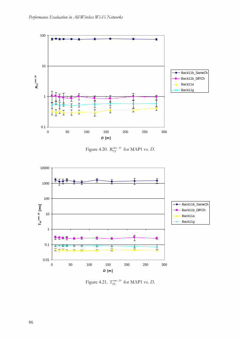
Performance Evaluation in All-Wireless Wi-Fi Networks
86
0.1
1
10
100
0 50 100 150 200 250 300
D [m]
RT
Xc
um
_1
0
Back11b_SameCh
Back11b_DiffCh
Back11a
Back11g
Figure 4.20. 10cum _
TXR for MAP1 vs. D.
0.01
0.1
1
10
100
1000
10000
0 50 100 150 200 250 300
D [m]
TD
Lc
um
_1
0 [
ms] Back11b_SameCh
Back11b_DiffCh
Back11a
Back11g
Figure 4.21. _10cum
DLT for MAP1 vs. D.
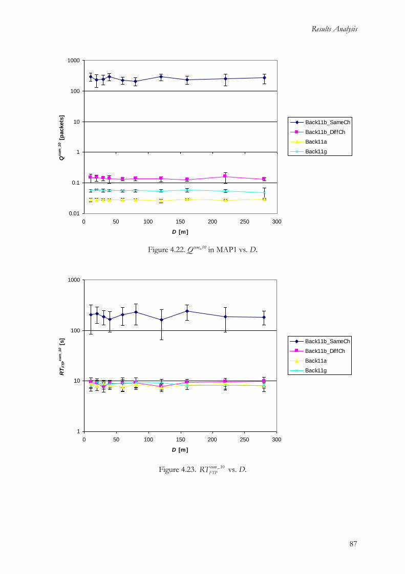
Results Analysis
87
0.01
0.1
1
10
100
1000
0 50 100 150 200 250 300
D [m]
Qc
um
_1
0 [
packets
]
Back11b_SameCh
Back11b_DiffCh
Back11a
Back11g
Figure 4.22. Qcum_10 in MAP1 vs. D.
1
10
100
1000
0 50 100 150 200 250 300
D [m]
RT
FT
Pc
um
_1
0 [
s]
Back11b_SameCh
Back11b_DiffCh
Back11a
Back11g
Figure 4.23. 10cum _
FTPRT vs. D.

Performance Evaluation in All-Wireless Wi-Fi Networks
88
1
10
100
1000
10000
0 50 100 150 200 250 300
D [m]
EV
oIP
cu
m_
10 [
ms]
Back11b_SameCh
Back11b_DiffCh
Back11a
Back11g
Figure 4.24. 10cum _
VoIPE vs. D.
Considering the free-space model and the link budget expression, it is possible to obtain the
maximum distance between MAPs for which the received power is greater than the receiver
sensitivity, when transmitting at a specific power level. These values are presented in Table 4.13,
for a combination of default receiver sensitivity (-95 dBm), maximum allowed sensitivity at the
default nominal data rate (-76 dBm for 802.11b and g, and -79 dBm for 802.11a), default
transmission power (5 mW), and maximum allowed transmission power (100 mW).
Table 4.13. Calculated maximum distance between MAPs.
Standard Transmit Power
[mW] Receiver Sensitivity
[dBm] Distance [m]
802.11b and g 5 -95 1250
802.11a 5 -95 600
802.11b and g 5 -76 140
802.11a 5 -79 95
802.11b and g 100 -76 628
802.11a 100 -79 425
Values in the first two rows are in accordance with the observations in Figure 4.19 to Figure 4.24,
since all values of D are well below the calculated distances. When receiver sensitivity is set to the
maximum allowed value, and keeping transmission power at 5 mW, the obtained distances are
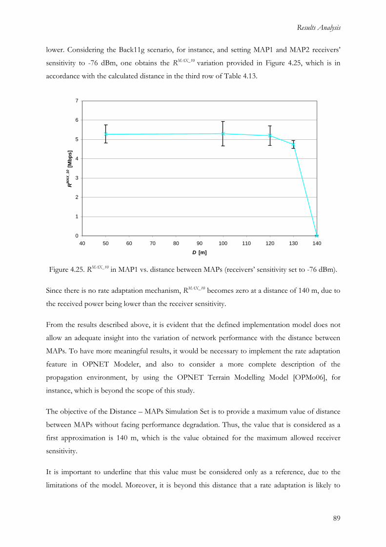
Results Analysis
89
lower. Considering the Back11g scenario, for instance, and setting MAP1 and MAP2 receivers’
sensitivity to -76 dBm, one obtains the RMAX_10 variation provided in Figure 4.25, which is in
accordance with the calculated distance in the third row of Table 4.13.
0
1
2
3
4
5
6
7
40 50 60 70 80 90 100 110 120 130 140
D [m]
RM
AX
_1
0 [
Mb
ps]
Figure 4.25. RMAX_10 in MAP1 vs. distance between MAPs (receivers’ sensitivity set to -76 dBm).
Since there is no rate adaptation mechanism, RMAX_10 becomes zero at a distance of 140 m, due to
the received power being lower than the receiver sensitivity.
From the results described above, it is evident that the defined implementation model does not
allow an adequate insight into the variation of network performance with the distance between
MAPs. To have more meaningful results, it would be necessary to implement the rate adaptation
feature in OPNET Modeler, and also to consider a more complete description of the
propagation environment, by using the OPNET Terrain Modelling Model [OPMo06], for
instance, which is beyond the scope of this study.
The objective of the Distance – MAPs Simulation Set is to provide a maximum value of distance
between MAPs without facing performance degradation. Thus, the value that is considered as a
first approximation is 140 m, which is the value obtained for the maximum allowed receiver
sensitivity.
It is important to underline that this value must be considered only as a reference, due to the
limitations of the model. Moreover, it is beyond this distance that a rate adaptation is likely to
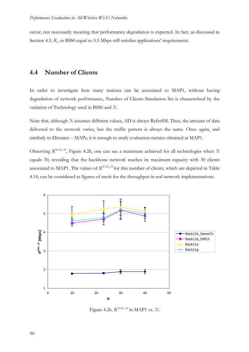
Performance Evaluation in All-Wireless Wi-Fi Networks
90
occur, not necessarily meaning that performance degradation is expected. In fact, as discussed in
Section 4.5, RN in BSS0 equal to 5.5 Mbps still satisfies applications’ requirements.
4.4 Number of Clients
In order to investigate how many stations can be associated to MAP1, without having
degradation of network performance, Number of Clients Simulation Set is characterised by the
variation of Technology used in BSS0 and N.
Note that, although N assumes different values, AD is always ReferSM. Thus, the amount of data
delivered to the network varies, but the traffic pattern is always the same. Once again, and
similarly to Distance – MAPs, it is enough to study evaluation metrics obtained at MAP1.
Observing RMAX_10, Figure 4.26, one can see a maximum achieved for all technologies when N
equals 30, revealing that the backbone network reaches its maximum capacity with 30 clients
associated to MAP1. The values of RMAX_10 for this number of clients, which are depicted in Table
4.14, can be considered as figures of merit for the throughput in real network implementations.
1
2
3
4
5
6
0 10 20 30 40 50
N
RM
AX
_10 [
Mb
ps]
Back11b_SameCh
Back11b_DiffCh
Back11a
Back11g
Figure 4.26. RMAX_10 in MAP1 vs. N.

Results Analysis
91
Table 4.14. Maximum throughput values at backbone network.
Technology used in BSS0 RMAX_10 @ N = 30
[Mbps]
Back11b_SameCh 1.88
Back11b_DiffCh 5.18
Back11a 5.35
Back11g 5.20
The high variation around RMAX_10 does not allow any further conclusion on the various
technologies. Thus, it is useful to use the relative gain definition to study the relative differences
among all technologies used in the backbone network. Figure 4.27 depicts GR, using (4.4), with x
representing Technology used in BSS0 and y representing N. It is possible to observe that a
maximum gain is obtained with N = 23 for Back11a, and with N = 30 for both Back11_DiffCh
and Back11g. If the criterion to determine the maximum number of clients would be the
maximisation of GR, Back11a should have a lower value than other scenarios, N = 23.
2.4
2.5
2.6
2.7
2.8
2.9
3.0
0 10 20 30 40 50
N
GR
Back11b_DiffCh
Back11a
Back11g
Figure 4.27. GR in MAP1 vs. N.
The other related backbone evaluation metrics (RTX, TDL and Q) do not give any new insight into
network performance. As expected, values of these statistics increase with N, as represented in
Figure 4.28, Figure 4.29 and Figure 4.30. A big difference is noticed between Back11b_SameCh
and the remaining technology settings, once more underlining that Back11b_SameCh represents
by far the worst case scenario.
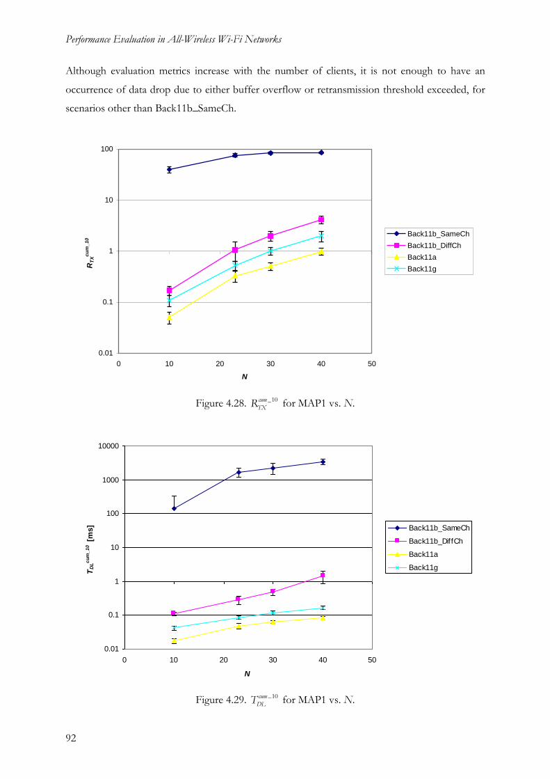
Performance Evaluation in All-Wireless Wi-Fi Networks
92
Although evaluation metrics increase with the number of clients, it is not enough to have an
occurrence of data drop due to either buffer overflow or retransmission threshold exceeded, for
scenarios other than Back11b_SameCh.
0.01
0.1
1
10
100
0 10 20 30 40 50
N
RT
Xc
um
_1
0
Back11b_SameCh
Back11b_DiffCh
Back11a
Back11g
Figure 4.28. 10cum _
TXR for MAP1 vs. N.
0.01
0.1
1
10
100
1000
10000
0 10 20 30 40 50
N
TD
Lc
um
_1
0 [
ms] Back11b_SameCh
Back11b_DiffCh
Back11a
Back11g
Figure 4.29. _10cum
DLT for MAP1 vs. N.

Results Analysis
93
0.001
0.01
0.1
1
10
100
1000
0 10 20 30 40 50
N
Qc
um
_1
0 [
packets
]
Back11b_SameCh
Back11b_DiffCh
Back11a
Back11g
Figure 4.30. Qcum_10 in MAP1 vs. N.
The overall degradation of backbone network performance for larger N is reflected in the
increase of non-real time applications response time and real time applications end-to-end delay,
as exemplified in Figure 4.31 and Figure 4.32, respectively. Nevertheless, for all simulated
situations, they are always within acceptable values (with the already known exception of scenario
Back11b_SameCh).
1
10
100
1000
0 10 20 30 40 50
N
RT
FT
Pc
um
_1
0 [
s]
Back11b_SameCh
Back11b_DiffCh
Back11a
Back11g
Figure 4.31. 10cum _
FTPRT vs. N.

Performance Evaluation in All-Wireless Wi-Fi Networks
94
10
100
1000
10000
0 10 20 30 40 50
N
EV
oIP
cu
m_10 [
ms]
Back11b_SameCh
Back11b_DiffCh
Back11a
Back11g
Figure 4.32. 10cum _
VoIPE vs. N.
Considering all previous results, the factor that determines the maximum number of clients
associated to MAP1 is the maximisation of R in the backbone network. Thus, 30 stations is the
higher value that N can assume without impairing network performance. Note that although
N = 23 maximises GR for Back11a, considering N = 30 does not have a significant impact on
applications performance.
4.5 Data Rate
The set of nominal data rates provided by both MAPs has a great impact on backbone network
performance. As pointed out in Subsection 3.1.2, it is important to investigate which data rates
can be used within BSS0. Simulation Set Data Rate is dedicated to this investigation, obtaining
results for the several values of Technology used in BSS0 and RN in BSS0 degrees of freedom.
Since the data rates provided by 802.11a do not have a correspondence to other standards,
scenario Back11a cannot be simulated with the above RN in BSS0 values. Instead, the following
values are used:
RN in BSS0 [Mbps] = 6; 12.

Results Analysis
95
The most important difference is the fact that 802.11a does not provide a 1 Mbps data rate. This
way, and to simplify results analysis, Back11a results are represented together with the other
scenarios.
RMAX_10 increases with the nominal data rate in BSS0, as expected, Figure 4.33. One interesting
observation is that the maximum throughput is closer to the theoretical data rate when RN in
BSS0 is equal to 1 Mbps. Once again, Back11b_SameCh presents the worst values for this and
the other evaluation metrics. In a similar way to previous sections, Back11b_SameCh values are
only considered as a reference to help on the task of interpreting other scenarios results.
0
1
2
3
4
5
6
0 1 2 3 4 5 6 7 8 9 10 11 12
R N in BSS0 [Mbps]
RM
AX
_10 [
Mb
ps]
Back11b_SameCh
Back11b_DiffCh
Back11a
Back11g
Figure 4.33. RMAX_10 in MAP1 vs. RN in BSS0.
Evaluation metrics RTX, TDL and Q reflect the lower throughput that the backbone network can
provide when configured with lower nominal data rates. As observed in Figure 4.34, Figure 4.35
and Figure 4.36, values for these three statistics are higher when RN in BSS0 is equal to 1 Mbps.
The higher Q value is even enough to give rise to dropped data due to buffer overflow, for
scenarios other than Back11b_SameCh, Figure 4.37.
Besides the occurrence of data drop, Figure 4.38 (FTP) and Figure 4.39 (VoIP) show that the
overall applications performance is greatly affected by backbone network operation when the
nominal throughput is 1 Mbps.

Performance Evaluation in All-Wireless Wi-Fi Networks
96
0.1
1
10
100
0 1 2 3 4 5 6 7 8 9 10 11 12
R N in BSS0 [Mbps]
RT
Xcu
m_10
Back11b_SameCh
Back11b_DiffCh
Back11a
Back11g
Figure 4.34. 10cum _
TXR for MAP1 vs. RN in BSS0.
0.01
0.1
1
10
100
1000
10000
0 1 2 3 4 5 6 7 8 9 10 11 12
R N in BSS0 [Mbps]
TD
Lcu
m_10 [
ms]
Back11b_SameCh
Back11b_DiffCh
Back11a
Back11g
Figure 4.35. _10cum
DLT for MAP1 vs. RN in BSS0.

Results Analysis
97
0.01
0.1
1
10
100
1000
0 1 2 3 4 5 6 7 8 9 10 11 12
R N in BSS0 [Mbps]
Qc
um
_1
0 [
packets
]
Back11b_SameCh
Back11b_DiffCh
Back11a
Back11g
Figure 4.36. Qcum_10 in MAP1 vs. RN in BSS0.
100
1000
10000
0 1 2 3 4 5 6 7 8 9 10 11 12
R N in BSS0 [Mbps]
Db
ufc
um
_1
0 [
bp
s]
Back11b_SameCh
Back11b_DiffCh
Back11a
Back11g
Figure 4.37. 10cum _
bufD for MAP1 vs. RN in BSS0.

Performance Evaluation in All-Wireless Wi-Fi Networks
98
1
10
100
1000
10000
0 1 2 3 4 5 6 7 8 9 10 11 12
R N in BSS0 [Mbps]
RT
FT
Pcu
m_10 [
s]
Back11b_SameCh
Back11b_DiffCh
Back11a
Back11g
Figure 4.38. 10cum _
FTPRT vs. RN in BSS0.
10
100
1000
10000
0 1 2 3 4 5 6 7 8 9 10 11 12
R N in BSS0 [Mbps]
EV
oIP
cu
m_10 [
ms]
Back11b_SameCh
Back11b_DiffCh
Back11a
Back11g
Figure 4.39. 10cum _
VoIPE vs. RN in BSS0.
For scenarios Back11b_DiffCh, Back11a and Back11g, values of FTP response time and VoIP
end-to-end delay increase approximately one order of magnitude, when RN in BSS0 decreases

Results Analysis
99
from 5.5 to 1 Mbps. Indeed, 10cum _
FTPRT becomes greater than 100 s and 10cum _
VoIPE almost reaches 1 s
(765 ms for Back11b_DiffCh and 724 ms for Back11g).
The results analysed in this section show that 1 Mbps needs to be excluded as a possible nominal
data rate in BSS0. The other two simulated data rates, 5.5 and 11 Mbps, do not impair backbone
network performance. Note that although the evaluation metrics reflect network degradation
when 5.5 Mbps is used instead of 11 Mbps, applications performance is still within acceptable
values.
4.6 Buffer Size
The previous section shows that the size of the buffer where packets coming from higher layers
are queued assumes an important role in some particular situations. It shows that, for lower data
rates, the queue size can reach the full buffer capacity, leading to an occurrence of data drop,
thus, buffer size is one of the most important MAPs’ internal parameters.
Buffer Size Simulation Set intends to investigate whether or not this parameter imposes any
limitation on backbone performance, when the default nominal rate is used (11 Mbps).
The most important evaluation metrics when analysing this Simulation Set are Q and Dbuf, which
are represented in Figure 4.40 and Figure 4.41. For Back11b_SameCh, it is noticed that Q
increases with increasing Bf, revealing that higher layers deliver to MAPs MAC a number of
packets greater than its buffer capacity. For the remaining scenarios, Q does not present any
significant variation, only a slight decrease occurring for Back11b_DiffCh when Bf is equal to
64 kbits. In fact, the observation of a small data drop rate in this situation shows that 64 kbits
must not be considered as a possible Bf. Note, however, that this is not an important limitation of
the network, since APs with greater Bf are commercially available and easy to found [Cisc07].
All the other backbone related evaluation metrics do not present a significant variation with
buffer size, with the exception of the already known situation of Back11b_SameCh.
Moreover, the analysis of applications statistics also shows a stable behaviour, meaning that the
overall network performance is not affected by buffer size decrease. Figure 4.42 and Figure 4.43
exemplify this statement, showing FTP and VoIP results.

Performance Evaluation in All-Wireless Wi-Fi Networks
100
0.0
0.1
1.0
10.0
100.0
1000.0
0 200 400 600 800 1000 1200
B f [kbits]
Qc
um
_1
0 [
packets
]
Back11b_SameCh
Back11b_DiffCh
Back11a
Back11g
Figure 4.40. Qcum_10 in MAP1 vs. Bf.
1
10
100
1000
10000
0 200 400 600 800 1000 1200
B f [kbits]
Db
ufc
um
_1
0 [
bp
s]
Back11b_SameCh
Back11b_DiffCh
Back11a
Back11g
Figure 4.41. 10cum _
bufD for MAP1 vs. Bf..

Results Analysis
101
1
10
100
1000
0 200 400 600 800 1000 1200
B f [kbits]
RT
FT
Pc
um
_1
0 [
s]
Back11b_SameCh
Back11b_DiffCh
Back11a
Back11g
Figure 4.42. 10cum _
FTPRT vs. Bf.
1
10
100
1000
10000
0 200 400 600 800 1000 1200
B f [kbits]
EV
oIP
cu
m_
10 [
ms]
Back11b_SameCh
Back11b_DiffCh
Back11a
Back11g
Figure 4.43. 10cum _
VoIPE vs. Bf.

Performance Evaluation in All-Wireless Wi-Fi Networks
102
4.7 Wired vs. Wireless Backbone
Results obtained in previous sections show that, for distances between MAPs below 140 m, the
maximum throughput that the backbone network can provide is 5.35 Mbps, obtained with the
802.11a standard.
As discussed in Section 2.4, one of the most widely used technologies to provide broadband
access to Internet is ADSL. Due to some intrinsic limitations, this type of technology has a
limited range, as illustrated in Figure 4.44 for ADSL2 and ADSL2plus.
Figure 4.44. ADSL2 and ADSL2plus maximum downstream data rates (extracted from
[DSLF03]).
For distances of 140 m (i.e., 460 feet, since 1 feet = 0.304 m), it is shown that ADSL technologies
are still able to provide the maximum data rates, which are greater than the values obtained with a
wireless backbone. Thus, in the perspective of an all-wireless Internet, some protocol and
architecture enhancements are needed. To obtain wired-like throughputs it is not enough to
deploy a mesh network topology using the existing 802.11 standards. But, one should keep in
mind that a wireless backbone requires no infrastructure deployment.

Conclusions
103
Chapter 5
Conclusions
5 Conclusions
This chapter finalises this work, summarising all the results obtained for each Simulation Set, and
pointing out the overall conclusions. Moreover, some considerations on future work are also
presented.

Performance Evaluation in All-Wireless Wi-Fi Networks
104
In the context of an increasing demand on mesh network investigation, several studies can be
found in literature addressing several important issues, such as: backbone networking, mesh
topology creation, routing, security and QoS. An overview on all of them in provided, describing
some important related studies, together with a description of the already available commercial
products providing mesh networking solutions. In parallel with these investigation efforts, is the
standardisation work of IEEE 802.11 TGs, aiming at standardising a mesh WLAN as a network
of interconnected APs [IEEE07a].
From all the ongoing research projects on mesh networks, WIP [WIPw07], under the European
R&D IST Work Programme in FP6, is one of the most prominent ones. WIP’s objective is the
development of an all-wireless Internet, using all mesh networks’ capabilities to establish a new
communications infrastructure, the so-called Radio Internet (where access and backbone
networks are wireless). To study the capacity of such a network, and to obtain guidelines for the
necessary enhancements, one must rely on some basic assumptions, which are obtained from a
simplified analysis of the network building blocks.
The objective of the present study lies in the context of the previous statement: the generic goal
is to evaluate the impact of several parameters on a mesh network capacity and performance, not
at a global perspective but instead at a single hop level. The obtained conclusions can then be
used as inputs to more complex studies, such as WIP.
Specifically, the impact of the following parameters is considered:
802.11 standard used within the backbone network.
The traffic mix delivered to the network.
Distance between MAPs.
Number of client stations associated to each MAP.
Data rate in backbone network.
Internal buffer size of MAPs.
To address the previous topics, a specific Implementation Model, with several degrees of
freedom, was defined, containing two MAPs with two RIs each, in order to allow the definition
of three BSSs (BSS0 for the backbone; BSS1 and BSS2 for the access network). The 802.11b
standard was used in BSS1 and BSS2, with a data rate of 11 Mbps. This generic Model was
implemented in OPNET Modeler, which was the selected simulation tool. The impact of the
previous parameters was analysed by running several Simulation Sets, Table 5.1, each one being
characterised by the variation of two specific network degrees of freedom. Note that although

Conclusions
105
OPNET Modeler is an efficient discrete event simulator, the amount of events to process makes
each simulation a very time consuming task. The total number of simulations took approximately
238h 55m 15s to complete.
Table 5.1. Relation between Simulation Sets and degrees of freedom.
Simulation Set
Degree of Freedom
#1 #2
Name Values Name Values
Service Mix
Technology used in BSS0
Back11b_SameCh; Back11b_DiffCh;
Back11a; Back11g
Application Distribution –
AD
RTiCeSM; ReferSM; NRTCeSM; NoRTiSM
Distance – MAPs
Distance between MAP1 and MAP2 – D
[m]
10; 20; 30; 40; 60; 80; 120; 160; 220; 280
Number of Clients
Number of clients – N
10; 23; 30; 40
Data Rate Nominal data rate – RN – in BSS0 [Mbps]
1; 5.5; 11
Buffer Size Buffer size in MAP RI2 – Bf
[kbit]
64; 256; 1024
In terms of the Technology used in BSS0, Back11b_SameCh represents the worst case scenario,
using the same technology (802.11b) and channel on both backbone and access networks. Thus,
it was considered only as a reference, since it is well known that such a configuration does not
satisfy mesh network requirements. In Back11b_DiffCh, 802.11b is also used, but the radio
channels on the several BSSs are different, corresponding to the non-overlapping channels of the
standard. In Back11a and Back11g, 802.11a and g were used in BSS0, respectively.
Regarding AD values, RTiCeSM and ReferSM represent distributions with a prevalence of real
time oriented applications, while NRTCeSM and NoRTiSM are non-real time centric.
Each Simulation Set was evaluated by means of several evaluation metrics, all considered in
MAPs RI2, characterising the backbone network performance: Throughput (R), Retransmission
attempts (RTX), Media access delay (TDL), Queue size (Q), Data dropped due to buffer overflow
(Dbuf), and Data dropped due to retransmission threshold exceeded (Drtx). Moreover, other
evaluation metrics to assess applications performance were also considered: Response time (RT)
for non-real time applications, and End-to-end delay (E) for real time applications.

Performance Evaluation in All-Wireless Wi-Fi Networks
106
The Service Mix Simulation Set aimed at studying the impact of having different applications
distributions among client stations in the overall network performance. Moreover, the differences
between the several technologies used in BSS0 were also evaluated. It is observed that 6.13 Mbps
is the higher RMAX_10, obtained in Back11g with AD equal to NoRTiSM, while for AD equal to
ReferSM the obtained value was 5.27 Mbps, for Back11a. These observations, together with the
values of GR, support the conclusion that Back11a has better performance for ADs with more
real time applications, while Back11g is better for ADs with prevalence of non-real time.
This relation between technology performance and AD indicates that it would be interesting to
have a metric able to indicate if the service mix offered to the network by client stations is real
time or non-real time centric. It is observed that Prcvd satisfies this requirement. In fact, from the
obtained results, it is possible to consider that if Prcvd > 750 bytes, clients’ service mix is real time
centric, otherwise, non-real time applications prevail.
Observation of TDL, RTX and Q related figures reveals that Back11a is the scenario were values of
these evaluation metrics are smaller. This way, and despite the differences to Back11b_DiffCh
and Back11g not being significant, standard 802.11a can be elected as the default standard for the
backbone network.
Due to the identified OPNET Modeler limitations, Distance – MAPs Simulation Set does not
provide any new input, compared to the analysis using the free-space model and the receivers’
sensitivity values. Thus, as a first approximation, it is considered that a distance of 140 m
between MAPs does not impair network performance. This distance was obtained considering a
receivers’ sensitivity of -76 dBm, which is the maximum allowed by 802.11 standards.
Results obtained from the Number of Clients Simulation Set show that 30 is the maximum
number of clients associated to MAP1, without having performance degradation. The values
obtained for RMAX_10, reproduced in Table 5.2, can than be considered as figures of merit for the
throughput in real network implementations.
The use of 1 Mbps as the backbone nominal data rate (when 802.11b or g is used) must be
excluded, considering the results of Data Rate Simulation Set. When RN in BSS0 is set to
1 Mbps, an occurrence of data drop is observed, as well as the degradation of overall applications
performance. Indeed, 10cum _
FTPRT becomes greater than 100 s and 10cum _
VoIPE almost reaches 1 s
(765 ms for Back11b_DiffCh and 724 ms for Back11g).
The other two simulated data rates, 5.5 and 11 Mbps, do not impair backbone network

Conclusions
107
performance. Note that although evaluation metrics reflect the network degradation when 5.5
Mbps is used instead of 11 Mbps, applications performance is still within acceptable values.
Table 5.2. Maximum throughput values.
Technology used in BSS0 RMAX_10 @ N = 30
[Mbps]
Back11b_DiffCh 5.18
Back11a 5.35
Back11g 5.20
Finally, Buffer Size Simulation Set reveals that for Back11b_DiffCh, with Bf set to 64 kbits, a
small data drop rate occurs. Thus, 64 kbits must not be considered as a possible Bf, what is not an
important limitation of the network, since APs with greater Bf are commercially available and easy
to found.
As already mentioned, the previous results are useful, in the sense that they can be used as inputs
to more in-depth studies (WIP, for instance). Table 5.3 summarises the most important results,
which can be viewed as the basic requirements of mesh network deployment, using 802.11
standards on both access and backbone networks.
Table 5.3. Basic requirements of a mesh network.
Parameter Basis Requirement
Technology used in backbone 802.11a (default)
Distance between MAPs ≤ 140 m
Number of client stations associated to each MAP
≤ 30
Nominal data rate in backbone ≥ 5.5 Mbps
Buffer size of each MAP > 64 kbits
Considering the values provided in Table 5.3, a specific network performance is expected,
quantified by the figures of merit of Table 5.2, and a specific applications performance with
values for FTP response time (representing non-real time applications) in the order of 10 s, and
for VoIP end-to-end delay (representing real time applications) around 60 ms.
Any new network architecture or protocol enhancement can be measured in terms of the gain
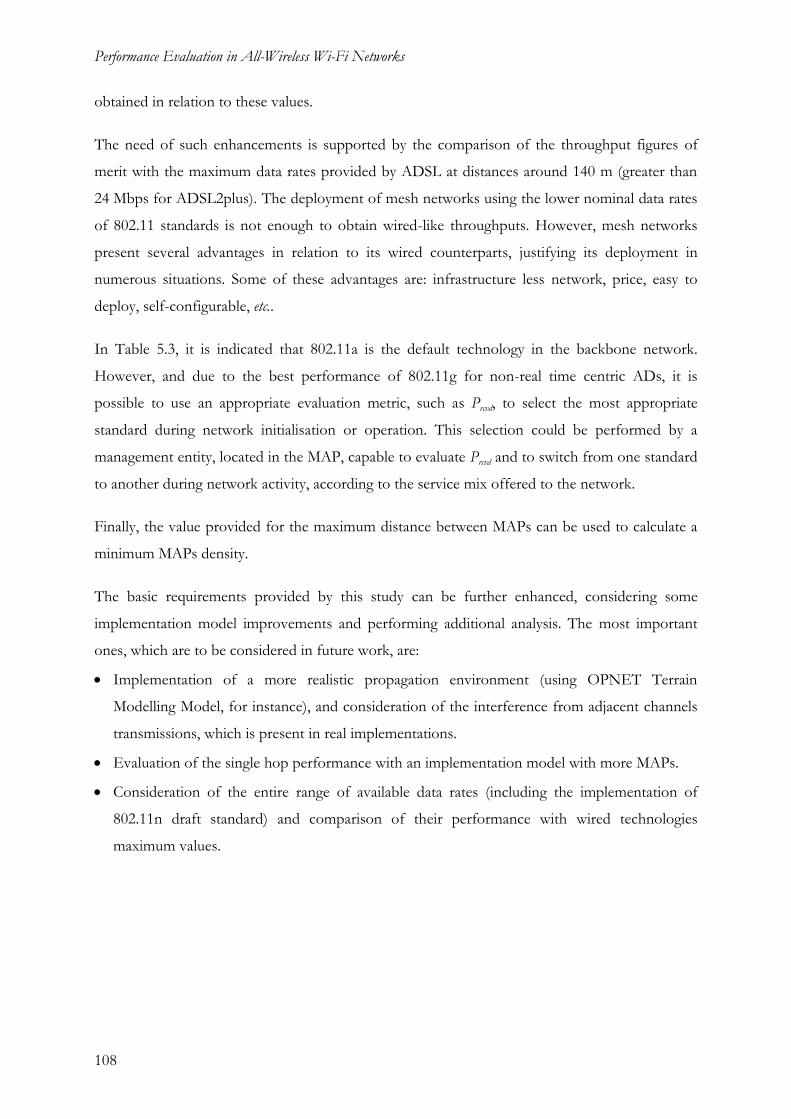
Performance Evaluation in All-Wireless Wi-Fi Networks
108
obtained in relation to these values.
The need of such enhancements is supported by the comparison of the throughput figures of
merit with the maximum data rates provided by ADSL at distances around 140 m (greater than
24 Mbps for ADSL2plus). The deployment of mesh networks using the lower nominal data rates
of 802.11 standards is not enough to obtain wired-like throughputs. However, mesh networks
present several advantages in relation to its wired counterparts, justifying its deployment in
numerous situations. Some of these advantages are: infrastructure less network, price, easy to
deploy, self-configurable, etc..
In Table 5.3, it is indicated that 802.11a is the default technology in the backbone network.
However, and due to the best performance of 802.11g for non-real time centric ADs, it is
possible to use an appropriate evaluation metric, such as Prcvd, to select the most appropriate
standard during network initialisation or operation. This selection could be performed by a
management entity, located in the MAP, capable to evaluate Prcvd and to switch from one standard
to another during network activity, according to the service mix offered to the network.
Finally, the value provided for the maximum distance between MAPs can be used to calculate a
minimum MAPs density.
The basic requirements provided by this study can be further enhanced, considering some
implementation model improvements and performing additional analysis. The most important
ones, which are to be considered in future work, are:
Implementation of a more realistic propagation environment (using OPNET Terrain
Modelling Model, for instance), and consideration of the interference from adjacent channels
transmissions, which is present in real implementations.
Evaluation of the single hop performance with an implementation model with more MAPs.
Consideration of the entire range of available data rates (including the implementation of
802.11n draft standard) and comparison of their performance with wired technologies
maximum values.

Annex A
109
Annex A
Applications Attributes
Annex A Applications Attributes
This annex describes the most important attributes characterising the applications that form the
service mix: FTP, E-mail, Web Browsing, Video Streaming, Video Conferencing and VoIP.
Client stations running these applications load the network with a mix of traffic that is
representative of all service classes. Moreover, values for each attribute used during simulation
runs are also provided.

Performance Evaluation in All-Wireless Wi-Fi Networks
110
Table A.1. FTP Attributes.
Attribute Definition Value
Command Mix (Get/Total)
Denotes the percentage of file "get" commands to the total FTP commands. The remaining percent of the commands are FTP file "put" transactions.
95%
Inter-Request Time [s]
Defines the amount of time between file transfers. The start time for a file transfer session is computed by adding the inter-request time to the time that the previous file transfer started.
exponential(600)
File Size [bytes] Defines the size in bytes of a file transfer. uniform_int(100000,
5000000)
Type of Service
Type of Service (ToS) assigned to packets sent from the client. It represents a session attribute which allows packets to be processed faster in IP queues. It is an integer between 0 - 252, 252 being the highest priority.
Best Effort(0)
Table A.2. E-mail attributes.
Attribute Definition Value in use
Send Interarrival Time [s]
Defines when the next email is sent. The start time of the next email is computed by adding the inter-arrival time to the time at which the previous email completed.
exponential(360)
Send Group Size
Defines the number of "queued emails" to be sent. uniform_int(1, 5)
Receive Interarrival Time [s]
Defines the amount of time between receiving emails. The start time for the next email reception is computed by adding the inter-arrival time to the time at which the previous emails were received.
exponential(360)
Receive Group Size
Defines the number of "queued emails" to be received. uniform_int(1, 5)
E-mail Size [bytes]
Defines the size in bytes of a 'typical' email. lognormal (100000,
660000)
Type of Service Same as Table A.1. Background(1)

Annex A
111
Table A.3. Web Browsing attributes.
Attribute Definition Value in use
HTTP Specification
Specifies HTTP parameters which are particular to the version of HTTP that is being used.
HTTP 1.1
Page Interarrival Time [s]
Defines the time in seconds between page requests. The start time for a page request is computed by adding the inter-arrival time to the time of the previous page request.
exponential(39.5)
Page Properties
Specifies the page properties. Each page contains many objects. Each object is represented by a row specification for this attribute.
Note: The first row represents the "page" itself, and the subsequent rows represent the objects within this page.
Refer to
Type of Service Same as Table A.1. Best Effort(0)
Table A.4. Web Browsing – Page Properties attribute.
Object Size [bytes] Number of Objects (objects per page)
Location
lognormal (20000, 50000) constant(1) HTTP Server
lognormal (14400,252000) gamma(47.258, 0.232) HTTP Server
Table A.5. Video Streaming attributes.
Attribute Definition Value in use
Incoming Stream Interarrival Time [s]
Defines the time in seconds between video frames in the incoming stream. The start time for an incoming video frame is computed by adding the inter-arrival time to the time the previous video frame completed.
constant(0.04)
Outgoing Stream Interarrival Time [s]
Defines the time in seconds between video frames in the outgoing stream. The start time for a new outgoing frame is computed by adding the inter-arrival time to the time that the pervious frame completed.
None
Incoming Stream Frame Size [bytes]
Defines the size in bytes of a single incoming video frame. constant(2000)
Outgoing Stream Frame Size [bytes]
Defines the size in bytes of a single outgoing video frame. constant(2000)
Type of Service Same as Table A.1. Streaming
Multimedia(4)

Performance Evaluation in All-Wireless Wi-Fi Networks
112
Table A.6. Video Conferencing attributes.
Attribute Definition Value in use
Incoming Stream Interarrival Time [s]
Same as Table A.5.
constant(0.0667)
Outgoing Stream Interarrival Time [s]
constant(0.0667)
Incoming Stream Frame Size [bytes]
constant(533)
Outgoing Stream Frame Size [bytes]
constant(533)
Type of Service Interactive Multimedia(5)
Table A.7. VoIP attributes.
Attribute Definition Value in use
Incoming Silent Length [s]
Defines the time in seconds spent in silence mode by the called party.
exponential(0.456)
Outgoing Silent Length [s]
Defines the time in seconds spent in silence mode by the calling party.
exponential(0.456)
Incoming Talk Spurt Length [s]
Defines the time in seconds spent in speech mode by the called party.
exponential(0.854)
Outgoing Talk Spurt Length [s]
Defines the time in seconds spent in speech mode by the calling party.
exponential(0.854)
Encoder Scheme
Encoder Scheme to be used by the calling and called party. G.729 A (silence)
Type of Service Same as Table A.1. Interactive Voice (6)
Compression Delay [s]
This attribute specifies the delay in compressing a voice packet. The total voice packet delay, called "analog-to-analog" or "mouth-to-ear", is given by:
delay = network_delay + encoding_delay + decoding_delay + compression_delay + decompression_delay
0.02
Decompression Delay [s]
This attribute specifies the delay in decompressing a voice packet. The total voice packet delay, called "analog-to-analog" or "mouth-to-ear", is given by:
delay = network_delay + encoding_delay + decoding_delay + compression_delay + decompression_delay
0.02

Annex B
113
Annex B
Results of Applications
Evaluation Metrics
Annex B Results of Applications Evaluation
Metrics
This annex presents the results of E-mail, Web Browsing and Video applications, obtained for
each Simulation Sets. It intends to be a complement of the FTP and VoIP results described in
Chapter 4.

Performance Evaluation in All-Wireless Wi-Fi Networks
114
0.1
1
10
100
1000
RTiCeSM ReferSM NRTCeSM NoRTiSM
AD
RT
ma
ilD
cu
m_
10[s
]
Back11b_SameCh
Back11b_DiffCh
Back11a
Back11g
Figure B.1. 10cum _
mailDRT vs. AD.
0.1
1
10
100
RTiCeSM ReferSM NRTCeSM NoRTiSM
AD
RT
we
bc
um
_1
0 [
s]
Back11b_SameCh
Back11b_DiffCh
Back11a
Back11g
Figure B.2. 10cum _
webRT vs. AD.

Annex B
115
1
10
100
1000
10000
RTiCeSM ReferSM NRTCeSM NoRTiSM
AD
Ev
ide
oc
um
_1
0 [m
s]
Back11b_SameCh
Back11b_DiffCh
Back11a
Back11g
Figure B.3. 10cum _
videoE vs. AD.
0.1
1
10
100
1000
0 20 40 60 80 100 120 140 160 180 200 220 240 260 280 300
D [m]
RT
ma
ilD
cu
m_
10 [
s]
Back11b_SameCh
Back11b_DiffCh
Back11a
Back11g
Figure B.4. 10cum _
mailDRT vs. D.

Performance Evaluation in All-Wireless Wi-Fi Networks
116
0.1
1
10
100
0 20 40 60 80 100 120 140 160 180 200 220 240 260 280 300
D [m]
RT
we
bc
um
_1
0 [
s]
Back11b_SameCh
Back11b_DiffCh
Back11a
Back11g
Figure B.5. 10cum _
webRT vs. D.
1
10
100
1000
10000
0 20 40 60 80 100 120 140 160 180 200 220 240 260 280 300
D [m]
Ev
ide
oc
um
_1
0 [
ms]
Back11b_SameCh
Back11b_DiffCh
Back11a
Back11g
Figure B.6. 10cum _
videoE vs. D.
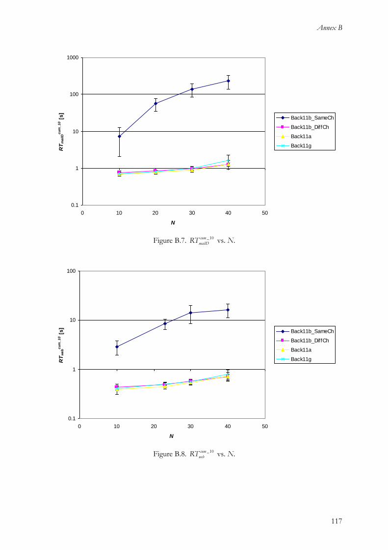
Annex B
117
0.1
1
10
100
1000
0 10 20 30 40 50
N
RT
ma
ilD
cu
m_
10 [
s]
Back11b_SameCh
Back11b_DiffCh
Back11a
Back11g
Figure B.7. 10cum _
mailDRT vs. N.
0.1
1
10
100
0 10 20 30 40 50
N
RT
we
bc
um
_1
0 [
s]
Back11b_SameCh
Back11b_DiffCh
Back11a
Back11g
Figure B.8. 10cum _
webRT vs. N.

Performance Evaluation in All-Wireless Wi-Fi Networks
118
0.1
1
10
100
1000
10000
0 10 20 30 40 50
N
Ev
ide
oc
um
_1
0 [
ms]
Back11b_SameCh
Back11b_DiffCh
Back11a
Back11g
Figure B.9. 10cum _
videoE vs. N.
0.1
1
10
100
1000
0 1 2 3 4 5 6 7 8 9 10 11 12
R N in BSS0 [Mbps]
RT
ma
ilD
cu
m_
10 [
s]
Back11b_SameCh
Back11b_DiffCh
Back11a
Back11g
Figure B.10. 10cum _
mailDRT vs. RN in BSS0.
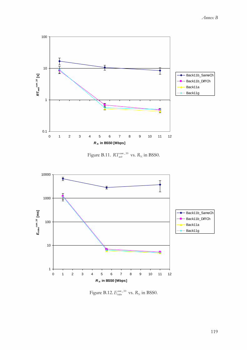
Annex B
119
0.1
1
10
100
0 1 2 3 4 5 6 7 8 9 10 11 12
R N in BSS0 [Mbps]
RT
we
bc
um
_1
0 [s
] Back11b_SameCh
Back11b_DiffCh
Back11a
Back11g
Figure B.11. 10cum _
webRT vs. RN in BSS0.
1
10
100
1000
10000
0 1 2 3 4 5 6 7 8 9 10 11 12
R N in BSS0 [Mbps]
Ev
ide
oc
um
_1
0 [
ms]
Back11b_SameCh
Back11b_DiffCh
Back11a
Back11g
Figure B.12. 10cum _
videoE vs. RN in BSS0.

Performance Evaluation in All-Wireless Wi-Fi Networks
120
0.1
1
10
100
1000
0 200 400 600 800 1000 1200
B f [kbits]
RT
ma
ilD
cu
m_
10 [
s]
Back11b_SameCh
Back11b_DiffCh
Back11a
Back11g
Figure B.13. 10cum _
mailDRT vs. Bf.
0.1
1
10
100
0 200 400 600 800 1000 1200
B f [kbits]
RT
web
cu
m_
10 [
s]
Back11b_SameCh
Back11b_DiffCh
Back11a
Back11g
Figure B.14. 10cum _
webRT vs. Bf.
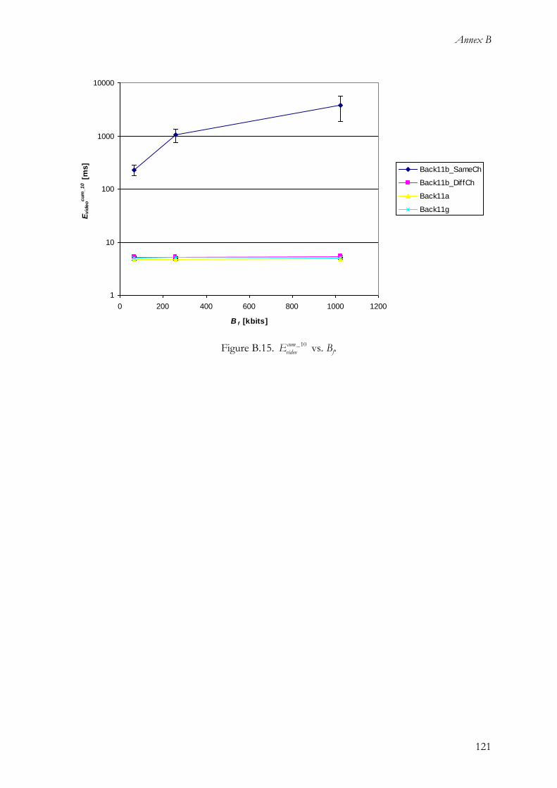
Annex B
121
1
10
100
1000
10000
0 200 400 600 800 1000 1200
B f [kbits]
Ev
ide
oc
um
_1
0 [
ms]
Back11b_SameCh
Back11b_DiffCh
Back11a
Back11g
Figure B.15. 10cum _
videoE vs. Bf.


References
123
References
References
[3GPP06a] 3GPP, Services and service capabilities, Report TS 22.105, V8.1.0, Sep. 2006
(http://www.3gpp.org).
[3GPP06b] 3GPP, Quality of Service (QoS) concept and architecture, Report TS 23.107, V6.4.0, Mar.
2006 (http://www.3gpp.org).
[AkWa05] Akyildiz,I., Wang,X., Wang,W., “Wireless Mesh Networks: a Survey”, Computer
Networks, Vol. 47, No. 4, pp. 445-487, Mar. 2005.
[BeAr07] BelAir Networks (http://www.belairnetworks.com/).
[Cisc07] Cisco Systems, Cisco Aironet Wireless Access Points – Solution Overview, 2007
(http://www.cisco.com).
[DSLF03] DSL Forum, ADSL2 and ADSL2plus – The new ADSL standards, White Paper, Mar.
2003 (http://www.dslforum.org/).
[DSLF07] DSL Forum (http://www.dslforum.org/).
[FAMZ03] Fitzek,F., Angelini,D., Mazzini,G. and Zorzi,M., “Design and Performance of an
Enhanced IEEE 802.11 MAC Protocol for Multihop Coverage Extension” IEEE
Wireless Communications, Vol. 10, No. 6, Dec. 2003, pp. 30-39.
[Fdid07] Fdida,S. (ed.), An All-Wireless Mobile Network Architecture, IST-WIP Project, Mar. 2005
(http://www.ist-wip.org).
[Fire07] Firetide, Inc. (http://www.firetide.com/).
[FWKD06] Faccin,S., Wijting,C., Kneckt,J. and Damle,A., “Mesh WLAN Networks: Concepts
and System Design”, IEEE Wireless Communications, Vol. 13, No. 2, Apr. 2006, pp.
10-17.
[HsSi02] Hsieh,H. and Sivakumar,R., “IEEE 802.11 over Multi-hop Wireless Networks:

124
Problems and New Perspectives”, in Proceedings of VTC’02 Fall – 56thVehicular
Technology Conference, Vancouver, BC, Canada, Sep. 2002.
[IEEE99] ANSI/IEEE, Wireless LAN Medium Access Control (MAC) and Physical Layer (PHY)
Specifications, Std. 802.11, 2003 (http://www.ieee.org).
[IEEE99a] ANSI/IEEE, Wireless LAN Medium Access Control (MAC) and Physical Layer (PHY)
Specifications: High-speed Physical Layer in the 5 GHz Band, Std. 802.11a, 1999
(http://www.ieee.org).
[IEEE99b] ANSI/IEEE, Wireless LAN Medium Access Control (MAC) and Physical Layer (PHY)
Specifications: Higher-speed Physical Layer Extension in the 2.4 GHz Band, Std. 802.11b,
1999 (http://www.ieee.org).
[IEEE03] ANSI/IEEE, Wireless LAN Medium Access Control (MAC) and Physical Layer (PHY)
Specifications. Amendment 4: Further Higher Data Rate Extension in the 2.4 GHz Band, Std.
802.11g, 2003 (http://www.ieee.org).
[IEEE04] ANSI/IEEE, IEEE Standard for Local and Metropolitan Area Network. Media Access
Control (MAC) Bridges, Std. 802.1D, 2004 (http://www.ieee.org).
[IEEE07a] IEEE 802.11s Task Group (http://www.ieee802.org/11/Reports/tgs_update.htm).
[IEEE07b] ANSI/IEEE, Wireless LAN Medium Access Control (MAC) and Physical Layer (PHY)
Specifications. Amendment: Enhancements for Higher Throughput, Draft Std.
P802.11n/D2.00, 2007 (http://www.ieee.org).
[IETF07] IETF (Internet Engineering Task Force) MANET (Mobile Ad-hoc Networks)
(http://www.ietf.org/html.charters/manet-charter.html).
[ITUT03] ITU-T, General Recommendations on the transmission quality for an entire international telephone
connection – One-way transmission time, Recommendation G.114, 2003.
[JuRu06] Ju,H. and Rubin,I., “Backbone Topology Synthesis for Multiradio Mesh Networks”,
IEEE Journal on Selected Areas in Communications, Vol. 24, No. 11, Nov. 2006, pp. 2116-
2126.
[Karl04] Karlsson,P. (ed.), Target Scenarios specification: vision at project stage 1, IST-EVEREST
Project, Deliverable D05, Apr. 2004.

References
125
[Layl04] Layland,R., “Understanding Wi-Fi Performance”, Business Communications Review, Mar.
2004, pp. 34-37.
[LjDa06] Ljung,R. and Dahlen,A. (eds.), Target Scenarios specification: vision at project stage 1,
IST-AROMA Project, Deliverable D05, Apr. 2006.
[MhDy06] MeshDynamics (http://www.meshdynamics.com/).
[OPMo06] OPNET Modeler 12.0 Documentation, OPNET Technologies,Inc., Bethesda, MD, USA,
2006 (http://www.opnet.com/).
[OPNT07] OPNET Technologies (http://www.opnet.com/).
[PkHo07] PacketHop, Inc. (http://www.packethop.com/).
[RaCh05] Raniwala,A. and Chiueh,T., “Architecture and Algorithms for an IEEE 802.11-Based
Multi-Channel Wireless Mesh Network”, in Proceedings of INFOCOM’05 – 24th Annual
Joint Conference of the IEEE Computer and Communications Societies, Miami, FL, USA, Mar.
2005.
[RoLe05] Roshan,P. and Leary,J., 802.11 Wireless LAN Fundamentals, Cisco Press, Indianapolis,
IN, USA, 2005.
[Stal00] Stallings,W., Data and Computer Communications, Prentice Hall, Upper Saddle River, NJ,
USA, 2000.
[Stal04] Stallings,W., “IEEE 802.11: Wireless LANs from a to n”, IT Professional, Vol. 6,
No. 5, Sep. 2004, pp. 32-37.
[Stal05] Stallings,W., Wireless Communications & Networks, Pearson Prentice Hall, Upper Saddle
River, NJ, USA, 2005.
[StSy07] Strix Systems, Inc. (http://www.strixsystems.com/).
[Trop07] Tropos Networks (http://www.tropos.com/).
[TsCh05] Tsai,T. and Chen,J., “IEEE 802.11 MAC Protocol over Wireless Mesh Networks:
Problems and Perspectives”, in Proceedings of AINA’05 - 19th International Conference on
Advanced Information Networking and Applications, Taipe, Taiwan, Mar. 2005.

126
[VaHa05] Vanhatupa,T. and Hämäläinen,T., “Multihop IEEE 802.11b WLAN Performance
for VoIP”, in Proceedings of PIMRIC’06 – IEEE 17th International Symposium on Personal,
Indoor and Mobile Radio Communications, Helsinki, Finland, Sep. 2005.
[Vars03] Varshney,U., “The Status and Future of 802.11 Based WLANs”, Computer, Vol. 36,
No. 6, June 2003, pp. 102-105.
[WaMB06] Walke,B., Mangold,S. and Berlemann,L., IEEE 802 Wireless Systems – Protocols,
Multi-hop Mesh/Relaying, Performance and Spectrum Coexistence, John Wiley & Sons,
Chichester, UK, 2006.
[WiFi07] Wi-Fi Alliance (http://www.wi-fi.org/).
[WIPw07] WIP – An All-Wireless Mobile Network Architecture (http://www.ist-wip.org).
[XuSa04] Xu,S. and Saadawi,T., “Does the IEEE 802.11 MAC Protocol Work Well in
Multihop Wireless Ad Hoc Networks?”, IEEE Communications Magazine, Vol. 39, No.
6, June 2001, pp. 130-137.
[ZhWH06] Zhao,R., Walke,B. and Hiertz,G., “An Efficient IEEE 802.11 ESS Mesh Network
Supporting Quality-of-Service”, IEEE Journal on Selected Areas in Communications, Vol.
24, No. 11, Nov. 2006, pp. 2005-2017.