Performance characteristics of packed bed thermal

energy storage for solar thermal power plants

by Kenneth Guy Allen

Thesis presented in partial fulfilment of the requirements for the degree of

Master of Science in Engineering at the Faculty of Engineering University of Stellenbosch

Supervisor: Prof. Detlev G. Kröger

Department of Mechanical and Mechatronic Engineering

March 2010

i

Declaration

By submitting this thesis electronically, I declare that the entirety of the work contained therein is my own, original work, that I am the owner of the copyright thereof (unless to the extent explicitly otherwise stated) and that I have not previously in its entirety or in part submitted it for obtaining any qualification.

Signature of candidate 12th day of February 2010

Copyright © 2010 Stellenbosch University All rights reserved

ii

Abstract Solar energy is by far the greatest energy resource available to generate power. One of the difficulties of using solar energy is that it is not available 24 hours per day - some form of storage is required if electricity generation at night or during cloudy periods is necessary. If a combined cycle power plant is used to obtain higher efficiencies, and reduce the cost of electricity, storage will allow the secondary cycle to operate independently of the primary cycle. This study focuses on the use of packed beds of rock or slag, with air as a heat transfer medium, to store thermal energy in a solar thermal power plant at temperatures sufficiently high for a Rankine steam cycle. Experimental tests were done in a packed bed test section to determine the validity of existing equations and models for predicting the pressure drop and fluid temperatures during charging and discharging. Three different sets of rocks were tested, and the average size, specific heat capacity and density of each set were measured. Rock and slag samples were also thermally cycled between average temperatures of 30 ºC and 510 ºC in an oven. The classical pressure drop equation significantly under-predicts the pressure drop at particle Reynolds numbers lower than 3500. It appears that the pressure drop through a packed bed is proportional to the 1.8th power of the air flow speed at particle Reynolds numbers above about 500. The Effectiveness-NTU model combined with a variety of heat transfer correlations is able to predict the air temperature trend over the bed within 15 % of the measured temperature drop over the packed bed. Dolerite and granite rocks were also thermally cycled 125 times in an oven without breaking apart, and may be suitable for use as thermal storage media at temperatures of approximately 500 ºC. The required volume of a packed bed of 0.1 m particles to store the thermal energy from the exhaust of a 100 MWe gas turbine operating for 8 hours is predicted to be 24 × 103 m3, which should be sufficient to run a 25-30 MWe steam cycle for over 10 hours. This storage volume is of a similar magnitude to existing molten salt thermal storage.

iii

Opsomming Sonenergie is die grootste energiebron wat gebruik kan word vir krag opwekking. ‘n Probleem met die gebruik van sonenergie is dat die son nie 24 uur per dag skyn nie. Dit is dus nodig om die energie te stoor indien dit nodig sal wees om elektrisiteit te genereer wanneer die son nie skyn nie. ‘n Gekombineerde kringloop kan gebruik word om ‘n hoër benuttingsgraad te bereik en elektrisiteit goedkoper te maak. Dit sal dan moontlik wees om die termiese energie uit die primêre kringloop te stoor, wat die sekondêre kringloop onafhanklik van die primêre kringloop sal maak. Dié gevalle studie ondersoek die gebruik van ‘n slak-of-klipbed met lug as hitteoordragmedium, om te bepaal of dit moontlik is om hitte te stoor teen ‘n temperatuur wat hoog genoeg is om ‘n Rankine stoom kringloop te bedryf. Eksperimentele toetse is in ‘n toets-bed gedoen en die drukverandering oor die bed en die lug temperatuur is gemeet en vergelyk met voorspelde waardes van vergelykings en modelle in die literatuur. Drie soorte klippe was getoets. Die gemiddelde grootte, spesifieke hitte-kapasiteit en digtheid van elke soort klip is gemeet. Klip en slak monsters is ook siklies tussen temperature van 30 ºC en 510 ºC verkoel en verhit. Die klassieke drukverlies vergelyking gee laer waardes as wat gemeet is vir Reynolds nommers minder as 3500. Dit blyk dat die drukverlies deur ‘n klipbed afhanklik is van die lug vloeispoed tot die mag 1.8 as die Reynolds nommer groter as omtrent 500 is. Die ‘Effectiveness-NTU’ model gekombineerd met ‘n verskeidenheid van hitteoordragskoeffisiënte voorspel temperature binne 15 % van die gemete temperatuur verskil oor die bed. Doloriet en graniet klippe het 125 sikliese toetse ondergaan sonder om te breek, en is miskien gepas vir gebruik in ‘n klipbed by temperature van sowat 500 ºC Die voorspelde volume van ‘n klipbed wat uit 0.1 m klippe bestaan wat die termiese energie vir 8 ure uit die uitlaat van ‘n 100 MWe gasturbiene kan stoor, is 24 × 103 m3. Dit behoort genoeg te wees om ‘n 25 – 30 MWe stoom kringloop vir ten minste 10 ure te bedryf. Die volume is min of meer gelyk aan dié van gesmelte sout store wat alreeds gebou is.

iv

Acknowledgements My thanks to the following people in particular for their input: Prof Kröger for his guidance, numerous ideas, numerous questions and suggestions, the many things he has taught me, and the opportunity he has given me. My parents for their support both physically and spiritually, and the opportunities they have given me, not only over the past two years, but over my whole life. Mr Zietsman; Kelvin and Julian for the laboratory support work, including fabrication of the test section. Without them, this would have taken a great deal longer, if it happened at all. Tom Fluri for his help and input, and others who have collected rock samples and given input such as Prof Harms, Dr Blaine and Cynthia Sanchez-Garrido. Also to Sonia Woudberg and Prof du Plessis Nico-Ben J.V Rensburg and Ross Taylor for the manual labour and good-natured company they provided whilst collecting rock samples; also to Joey Rootman for getting permission for the collection of the granite from Welbedacht farm. JC Ruppersberg, Sewis van Zyl, Tim Bertrand, Andrew Gill and other postgraduate students for general help. Murray and Roberts for giving me a leave of absence to study. Also to Ramsay Brierley for his help. CRSES (SANERI) for funding. Somerset Sports for the loan of 1200 golf balls; Maties tennis for 300 tennis balls.

v

“And God made two great lights; The greater light to rule the day...”

Genesis 1:16

vi

Table of contents

Declaration .......................................................................................................i

Abstract........................................................................................................... ii

Opsomming .................................................................................................... iii

Acknowledgements.......................................................................................... iv

Table of contents.............................................................................................vi

Table of figures ................................................................................................x

List of tables..................................................................................................xiii

Nomenclature................................................................................................ xiv

1 INTRODUCTION........................................................................................1

1.1 BACKGROUND...........................................................................................1

1.2 OBJECTIVES..............................................................................................3

1.3 MOTIVATION ............................................................................................3

1.4 PREVIOUS WORK.......................................................................................4

1.4.1 Solar thermal power generation......................................................4

1.4.2 Thermal storage and packed beds ...................................................5

2 MATERIAL PROPERTIES AND DESIGN CONSIDERATIONS...... ..8

2.1 ROCK AND SLAG PROPERTIES....................................................................8

2.2 DESIGN CONSIDERATIONS.......................................................................10

2.3 EDGE EFFECTS OR WALL CHANNELLING..................................................14

2.4 THERMAL STORAGE DESIGN FIGURES FOR COMPARISON.........................15

3 POROUS MATERIALS AND PRESSURE DROP PREDICTION......16

3.1 POROUS MATERIALS................................................................................16

3.1.1 Homogeneous and heterogeneous .................................................16

3.1.2 Structure.........................................................................................16

3.1.3 Porosity..........................................................................................16

vii

3.2 REYNOLDS NUMBER AND PARTICLE SIZE DEFINITIONS............................17

3.2.1 Reynolds number definitions..........................................................17

3.2.2 Particle size definition ...................................................................18

3.3 PRESSURE DROP PREDICTION..................................................................19

3.3.1 The Darcy and Forchheimer flow regimes....................................20

3.3.2 The Ergun equation .......................................................................21

3.3.3 The Representative Unit Cell model (RUC) ..................................22

3.3.4 Equation of Singh et al...................................................................23

3.3.5 Present method ..............................................................................24

4 THERMAL MODELS...............................................................................28

4.1 SUMMARY OF PREVIOUS WORK...............................................................28

4.2 HEAT TRANSFER CORRELATIONS............................................................31

4.2.1 Void fraction / Reynolds number correlations...............................31

4.2.2 The Lévêque analogy (friction - heat transfer correlation)...........33

4.3 GOVERNING EQUATIONS.........................................................................35

4.3.1 The Schumann model and assumptions .........................................35

4.3.2 The Effectiveness - NTU method of Hughes ..................................38

4.3.3 Jeffreson particle conductivity adjustment ....................................39

4.3.4 Continuous Solid Phase (C-S) model.............................................40

5 EXPERIMENTAL AND ANALYTICAL METHOD................. ............41

5.1 APPARATUS: WIND TUNNEL LAYOUT AND TEST SECTION........................41

5.1.1 Weighted particle size, volume and density ...................................44

5.1.2 Void fraction ..................................................................................45

5.1.3 Specific heat capacity ....................................................................46

5.1.4 Thermal conductivity .....................................................................46

5.1.5 Thermal cycling resistance of rock samples ..................................46

5.2 NUMERICAL AND ANALYTICAL METHOD .................................................47

6 EXPERIMENTAL MEASUREMENTS AND PREDICTED RESULTS

......................................................................................................................49

viii

6.1 INITIAL TESTS AND FINDINGS..................................................................49

6.2 MEASURED ROCK PROPERTIES................................................................49

6.3 PRESSURE DROP......................................................................................51

6.3.1 Test section influence on pressure drop ........................................51

6.3.2 Comparison with predictions, repeatability and edge effects........51

6.3.3 Best fit present method...................................................................56

6.3.4 Comparison with a packed bed of spheres ....................................58

6.4 THERMAL CHARACTERISTICS..................................................................61

6.5 ROCK THERMAL CYCLING TESTS AT TEMPERATURES ABOVE 500 ºC .......67

7 LARGE PACKED BEDS ..........................................................................70

7.1 GEOMETRY .............................................................................................70

7.2 TEMPERATURE AND PRESSURE DROP PREDICTIONS FOR LARGE BEDS......71

8 CONCLUSIONS AND FURTHER WORK REQUIRED......................78

8.1 CONCLUSIONS FROM WORK DONE...........................................................78

8.2 RECOMMENDATIONS AND FURTHER WORK REQUIRED.............................79

9 REFERENCES ...........................................................................................81

APPENDIX A CALIBRATION AND INSTRUMENTATION...............A1

APPENDIX B APPARATUS AND ROCK SAMPLE PICTURES.........B1

APPENDIX C EQUATION MANIPULATION .......................................C1

THE HAGEN NUMBER AS A FUNCTION OF PRESSURE DROP..................................C1

EXPONENTIAL TEMPERATURE DISTRIBUTION FOR E-NTU MODEL .....................C1

APPENDIX D SOLUTION OF E-NTU NUMERICAL MODEL ...........D1

APPENDIX E MEASURING ROCK THERMAL CONDUCTIVITY ..E1

ix

APPENDIX F WIND TUNNEL MASS FLOW CALCULATION ......... F1

APPENDIX G ROCK DENSITY MEASUREMENTS ............................G1

APPENDIX H ADDITIONAL PRESSURE DROP MEASUREMENTS....

..............................................................................................H1

TEST SECTION INFLUENCE ON PRESSURE DROP MEASUREMENT..........................H1

EDGE EFFECTS AND REPEATABILITY OF THE 42 MM DOLERITE ...........................H2

APPENDIX I SAMPLE CALCULATIONS.................................................. I1

WIND TUNNEL MASS FLOW RATE........................................................................ I1

PRESSURE DROP CALCULATION........................................................................... I1

The Ergun equation ....................................................................................... I2

The RUC model.............................................................................................. I2

The correlation of Singh et al. .......................................................................I2

THE BEST FIT PRESENT METHOD FOR PRESSURE DROP......................................... I2

HEAT TRANSFER COEFFICIENT CALCULATION..................................................... I3

ROCK HEATING RATE IN OVEN: HEAT TRANSFER COEFFICIENT ESTIMATE............ I5

STEAM CYCLE POWER GENERATION.................................................................... I7

x

Table of figures Figure 1: Simplified schematic of proposed SUNSPOT cycle (Fluri, 2009; partly

based on Quaschning et al., 2002)............................................................2 Figure 2: Effect of stone size on absorption of heat; thermally long or short

packing during discharge (from Sanderson and Cunningham, 1995a)...11 Figure 3: Diagram of RUC ....................................................................................22 Figure 4: Wind tunnel layout (based on Kröger, 2004).........................................41 Figure 5: Thermocouple positions .........................................................................42 Figure 6: Dimensions of test section without wall lining ......................................43 Figure 7: Shale: density measurement ...................................................................50 Figure 8: 43 mm shale : edge effects and repeatability (Ta : 23 ºC; pa : 100.3 kPa;

padded Acs≈ 0.435×0.460 m2) ................................................................52 Figure 9: 66 mm granite: edge effects and repeatability (Ta : 24 ºC; pa : 100.4 kPa)

................................................................................................................53 Figure 10: 43 mm shale pressure drop detail .........................................................53 Figure 11: RUC model comparison with measured pressure drop........................54 Figure 12: Comparison with correlation of Singh et al. (2006).............................55 Figure 13: Comparison of particle dimension definition (shale; Ta : 23 ºC; pa :

100.3 kPa) ...............................................................................................55 Figure 14: c2 as a function of pore Reynolds number (43 mm shale, repacked) ...56 Figure 15: c2 as a function of pore Reynolds number (66 mm granite, repacked) 56 Figure 16: 43 mm shale – present method.............................................................57 Figure 17: 42 mm dolerite – present method.........................................................57 Figure 18: 66 mm granite (repacked) – present method........................................58 Figure 19: Comparison with a bed of 42.6 mm spheres (golf balls) .....................59 Figure 20: Kays and London (1984) friction factor for a bed of spheres, ε ≈ 0.38

................................................................................................................59 Figure 21: Components of the Ergun equation compared with the correlation of

Singh et al. and measurements from the repacked shale ........................60 Figure 22: Altered turbulent term in the Ergun equation.......................................61 Figure 23: Mid bed fluid temperatures: predicted and measured (shale,

Martin/GLE heat transfer correlation and Hughes E-NTU method) ......62 Figure 24: Bed exit fluid temperatures: predicted and measured (shale,

Martin/GLE heat transfer correlation and Hughes E-NTU method) ......62 Figure 25: 43 mm shale, discharging, 0.0940 kg/s (0.470 kg/m2s) .......................63 Figure 26: Comparison of heat transfer coefficient correlations (shale, 0.297

kg/m2s)....................................................................................................64 Figure 27: Comparison of Martin GLE air outlet temperature predictions for

Ergun predicted and measured pressure drop (43 mm shale, 0.297 kg/m2s)....................................................................................................64

xi

Figure 28: Temperature of a sphere cooled in a fluid at 25 ºC (BiD ≈ 0.4) ...........65 Figure 29: Effect of thermal conductivity on predicted fluid temperatures

(dolerite, 0.365 kg/m2s, Martin GLE, xf=0.45) ......................................65 Figure 30: 66 mm granite air temperatures (charging, 0.321 kg/m2s)...................66 Figure 31: 42 mm dolerite air temperatures (charging, 0.365 kg/m2s)..................67 Figure 32: Structural failure of shale above 500 ºC...............................................69 Figure 33: Fragmented slag sample after 60 cycles...............................................69 Figure 34: Fragmented quartz sample after 30 cycles...........................................69 Figure 35: Dolerite explosive failure during first heating .....................................69 Figure 36: Hairline fracture of dolerite after 110 cycles .......................................69 Figure 37: Granite after 110 cycles........................................................................69 Figure 38: Slag packed in a conical mound as in Curto and Stern (1980) ............70 Figure 39: Cross-sectional bed layout with charging air-flow direction ...............70 Figure 40: Additional ducts for charging sections of the bed................................71 Figure 41: Cross-section of alternative horizontal bed layout...............................71 Figure 42: Cross-sectional area of bed to reduce thermal losses...........................71 Figure 43: Air discharge temperatures for 0.2 m rock (L = 23 m; G = 0.14 kg/m2s)

................................................................................................................74 Figure 44: Comparison of rock size effect on air outlet temperature during

discharge of packed bed at 0.14 kg/m2s (224 kg/s, air inlet temperature 25 ºC) ......................................................................................................74

Figure 45: Pressure drop during charging of bed for different rock sizes .............76 Figure 46: Solid temperature profile at different positions in a bed of 0.05 m rocks

................................................................................................................77 Figure 47: Nozzle pressure transducer (Channel 17; p = 2600.9V - 2501.6) .......A1 Figure 48: Nozzle upstream pressure transducer (Channel 18; p = 2603.1V - 2500)

...............................................................................................................A2 Figure 49: Packed bed pressure transducer calibration (Channel 19; p = 637.35V –

637.22) ...................................................................................................A2 Figure 50: Comparison of thermocouple readings with a thermometer ...............A3 Figure 51: Wind tunnel wall insulation with mixer visible ..................................B1 Figure 52: Namibian shale in test section.............................................................B1 Figure 53: Calvinian granite in test section ..........................................................B2 Figure 54: Edge effect reduction ..........................................................................B2 Figure 55: Time step independence, 43 mm shale, 0.47 kg/m2s ..........................D1 Figure 56: Segment size independence, 100 mm rocks, 0.19 kg/m2s...................D2 Figure 57: Divided bar apparatus (Jones, 2003) ................................................... E1 Figure 58: Granite: density measurement.............................................................G1 Figure 59: Dolerite: density measurement............................................................G1 Figure 60: Empty box pressure drop (Ta : 20 ºC; pa : 100.44 ×103 N/m2)............H1 Figure 61: Box effect on measured pressure drop (43 mm shale, repacked; Ta : 23

ºC; pa : 100.7 ×103 N/m2).......................................................................H2

xii

Figure 62: Edge effects and repeatability for 42 mm dolerite ..............................H2

xiii

List of tables Table 1: Sample rock density and thermal conductivity at 27 ºC (Özkahraman et

al. 2004)....................................................................................................9 Table 2: South African rock properties (25 ºC, Jones, 2003) ..................................9 Table 3: Material density, conductivity and specific heat capacity (332.5 ºC,

Dinter, 1992)...........................................................................................10 Table 4: Measured and calculated rock properties ................................................50 Table 5: Summary of shale dimensions.................................................................51 Table 6: Best fit values of c and c2 ........................................................................57 Table 7: Rock thermal conductivity for numerical analysis ..................................61 Table 8: Values used for calculating large bed performance.................................72 Table 9: Packed bed characteristics (Acs = 40 × 40 m2) ........................................75 Table 10: Typical bed power and energy requirements for 8 hours charging .......77 Table 11: Wind tunnel nozzle sizes ...................................................................... F1 Table 12: Input values for mass flow rate calculation ........................................... I1 Table 13: Input values for pressure drop calculation............................................. I2 Table 14: Input values best fit present method ...................................................... I3 Table 15: Values to calculate heat transfer parameters ......................................... I3

xiv

Nomenclature Acs cross-sectional area of test section perpendicular to flow direction, m2 An cross-sectional area of mass flow nozzle, m2 Avs specific surface area of particles (ratio of total surface area of particles to

volume of solid particles) m-1 As total surface area of solid particles in bed/RUC volume, m2 Atus cross-sectional area upstream of mass flow nozzle, m2 a particle surface area per unit volume of whole packed bed, m-1 B particle conductivity adjustment term of Sagara and Nakahara (1991) BiD Biot number, hD/2ks b constant for power law viscosity approximation gTf

b (0.683) Cn nozzle coefficient of discharge, for mass flow correlation cd drag coefficient for a packed bed, as used in the RUC model cpf specific heat capacity of fluid at constant pressure, J/kgK cvf specific heat capacity of fluid at constant volume, J/kgK cs specific heat capacity of rock/solid, J/kgK cw specific heat capacity of water, J/kgK c friction factor coefficient for present method pressure drop fit c2 coefficient for present method pressure drop fit/estimation c3 coefficient for present method pumping power estimate D particle hydraulic/equivalent diameter or size, m d RUC model cube side length for whole RUC cube, m dh generalised hydraulic diameter, m di particle size of particle i, m ds RUC model solid cube side length, m dt bed diameter/hydraulic diameter, m eeff effectiveness of heat exchanger F drag factor of Du Plessis and Woudberg (2008) f friction factor as defined for present method in this study fer Ergun friction factor

fK friction factor of Kays and London g

shfK

gGf

2/2

σρ= , shσ is an equivalent

shear stress in the flow direction fs friction factor defined by Singh et al. (2006) G air mass flux, csf AmG /�= , kg/m2s

G dimensionless mass flux Gr Grashof number g constant for viscosity approximation gTf

b: 3.75 × 10-7 kg/m s Kb gg constant of gravitational acceleration, m/s2 Hg Hagen number h heat transfer coefficient (surface area), W/m2 hv volumetric heat transfer coefficient – product ha, W/m3

xv

hv* adjusted volumetric heat transfer coefficient, W/m3

K Darcy permeability coefficient, m2 kef effective thermal conductivity of fluid for C-S model, W/mK kes effective thermal conductivity of solid packing in bed, C-S model, W/mK kf fluid thermal conductivity, W/mK ks Rock/solid thermal conductivity, W/mK L flow-wise length of the bed, m Le estimated tortuous flow length through packed bed, m Lf GLE characteristic length, m l general characteristic length of object (as used in Re or Bi), m

fm� mass flow rate of fluid flowing through bed cross section, kg/s

ms mass of solid, kg msseg mass of solid in discrete segment, kg mw mass of water, kg Nu Nusselt number NTU number of transfer units NTUc adjusted NTU value from correlation of Jeffreson NTU* adjusted NTU value from correlation of Sagara and Nakahara n number of spheres in a given control volume ni number of particles of size di

Pe Peclet number Pe electrical pumping power required, W Pp pumping hydraulic power, W Pr fluid Prandtl number Pw wetted perimeter, m pa ambient pressure, N/m2 pup pressure upstream of mass flow nozzle, N/m2 ∆ pn pressure drop over mass flow nozzle, N/m2

Lp /∆ pressure gradient (generally over a packed bed), N/m2/m

Q� heat flow rate, W

maxQ� maximum possible heat transfer rate between air and rock, W

totQ total heat flowing into packed bed in a given time, J

R Ideal gas constant, 287 J/kgK (for air) Ra Rayleigh number, Ra = GrPr Re generalised Reynolds number or pore Reynolds number Re /f b t fu dρ µ=

Reer Ergun definition of the Reynolds number Re /[ (1 )]er f s fv Dρ µ ε= −

ReK Kays and London Reynolds number A

LGA

f

csK µ

ε4Re = ; A is the total heat

transfer area Ren mass flow nozzle Reynolds number Re /n n n n nv dρ µ=

Rep particle Reynolds number fsfp Dv µρ /Re =

Ta ambient temperature, ºC

xvi

Tenv ambient/surrounding temperature, °C Tf fluid/air temperature, °C Tfilm average film temperature of fluid surrounding an object, ºC To initial bed temperature before charging, ºC Tov oven temperature for thermal cycling tests of rocks, ºC Ts solid/rock temperature, °C t time, s ∆ t time interval for finite difference numerical solution, s U overall thermal loss coefficient for a packed bed, W/m2K ub average interstitial air speed in voids/pores between rocks, m/s V� air volume flow rate through packed bed, m3/s Vbed volume of packed bed, m3 Vf void volume in sample / RUC, m3 VH ratio of solid to fluid thermal capacitance Vo total sample volume / total RUC volume, m3 Vs solid volume in sample / RUC, m3 v speed of temperature wave through packed bed, m/s vn air speed in wind tunnel flow nozzle, m/s vs superficial speed through porous medium, m/s Wp Pumping energy through packed bed, J wi mass fraction of particle i in a selection of particles x co-ordinate in flow direction, m xf frictional fraction of total pressure drop ∆x discrete segment length of bed, m Y approach velocity factor for mass flow correlation z constant to determine friction factor in present method Greek letters α thermal diffusivity, m2s

axα axial fluid thermal dispersion coefficient, m2/s

β volumetric coefficient of expansion of fluid, 1/K ε void fraction (porosity) of a material

rε emissivity (radiated heat)

η ( )

1x

NTULe

∆−−

fanη efficiency of fan (to blow air through bed)

motorη efficiency of electric motor to drive fan

λ dynamic performance factor of Torab and Beasley (1987)

fµ fluid (dynamic) viscosity, kg/ms

nµ fluid viscosity at mass flow nozzle, kg/ms

υ fluid (kinematic) viscosity, m2/s ρf density, kg/m3

xvii

ρn air density at mass flow nozzle, kg/m3 ρs rock/solid density, kg/m3 σ Boltzmann constant, 5.67 × 10-8 W/m2K4

τ time constant of a packed bed (1 )s s cs s s

f pf f pf

c A L m c

m c m c

ρ ε− =� �

, s

oτ time to charge a given packed bed, s

φ availability in bed, J

gφ gas expansion factor for mass flow correlation

ψ sphericity of particle, /s eA a

Subscripts and superscripts i condition of a particular segment or particle f fluid condition/property/characteristic n reference to condition or property at wind tunnel mass flow nozzle s solid condition/property/characteristic + condition at next time step Abbreviations E – NTU Hughes effectiveness - NTU analytical thermal model GLE Generalised Lévêque Equation RUC representative unit cell (analytical model for pressure drop)

1

1 Introduction It is becoming increasingly necessary for countries to obtain power from sources other than conventional fossil fuels. This is as a consequence of an increasing population, people becoming more aware of environmental constraints, and the rising cost of conventional fuels. Nuclear and renewable energy sources will have to provide an increasing percentage of total power capacity. Nuclear power is still reliant on limited sources of fuel, and has strong environmental and political implications, limitations by which renewable energy is generally unaffected. It therefore makes sense to consider renewable energy sources as a means of power generation. The largest supply of renewable energy is in the form of solar energy. There are, at present, two different ways of converting incident solar light into electrical power: solar thermal, where the sun’s light is captured as heat; and photovoltaic, where the light is used to produce electricity by means of semiconductors. The intention of this study is to determine the feasibility of using packed beds of rocks to store thermal energy for solar thermal power plants. This chapter presents a brief background on solar energy and the need for storage. The objectives for the study are listed and motivated. A brief introduction to previous work completed on solar power plants, combined cycles and thermal storage is provided.

1.1 Background Solar thermal power plants are being built on a large scale in North America (The California Energy Commission [s.a]), Spain (Solar Millenium, 2009) and other countries. Interest in solar power generation is growing, and the technology is improving. South Africa has some of the best solar irradiation levels in the world (Fluri, 2009), which are not being used to their potential, as there are currently no concentrating solar power plants in use. ESKOM has a shortage of installed generating capacity, and solar power plants should be considered as an alternative power source. The major barrier to the construction of solar power plants is the high capital cost, and the area of land required for their use. However, it may be possible to somewhat reduce the required area and the overall cost by using a combined cycle plant, and developing new methods of storage, which would improve the plant efficiency and reduce costs. An example of such a cycle is the SUNSPOT (Stellenbosch UNiversity Solar Power Technology) cycle, proposed by Kröger (2008), shown in Figure 1.

2

The SUNSPOT cycle is a combined cycle - the primary cycle is a Brayton cycle gas turbine, while the secondary cycle is a Rankine steam cycle. Ambient air is compressed and heated to 800 ºC or more by means of solar heat in a central receiver, from where it passes to a gas turbine. If desired, a combustion chamber could be used to reduce temperature fluctuations from weather effects and also to allow the turbine to run when the sun is not available. It would also allow turbine inlet temperatures to be higher than 1000 ºC, which would allow for higher operating efficiencies. The remaining heat in the exhaust from the turbine (400 - 500 ºC) is stored in a storage volume (such as a rock or slag bed, where the turbine exhaust gas passes directly through the bed) for use in a boiler to produce steam for a typical steam cycle. Since solar thermal power plants will generally be situated in arid areas, where cooling water is scarce, dry-cooling of the steam cycle by means of air cooled condensers will be desirable. The advantage of storage is that the steam cycle could be run mostly at night, when ambient temperatures are lower than they are in the day and dry-cooling is more effective, resulting in higher turbine efficiencies. During periods of high demand, combustion of gas or other renewable fuel in the gas turbine may be used to provide additional power for a limited period.

Figure 1: Simplified schematic of proposed SUNSPOT cycle (Fluri, 2009; partly based on Quaschning et al., 2002) The problem with solar power is that it is intermittent – it is unavailable at night and every time a shadow is cast on the collection area, the power output is reduced. As a consequence of the intermittent supply, energy supply and demand curves do not necessarily match. For this reason it is desirable to store the energy to reduce the fluctuations, or supply it at a later stage when there is a demand. In solar thermal plants, the most feasible way to do this is to store the energy as heat before it is converted to electricity. Once converted to electricity, it is more difficult to store on a large scale unless there is a pumped storage scheme available. In the words of Spiga and Spiga (1982), “In solar electrical conversion,

3

the storage of large amounts of high-temperature energy is a key technology for the successful exploitation of this energy source on a significant scale.”. There are several different methods for storage of heat energy. It can be done with phase change materials (latent heat), or sensible heat storage in solids, liquids, gases or combinations of these. However, not all of these have been examined in detail, and there is scope for further work to improve them or test new applications.

1.2 Objectives In light of the need for thermal storage in solar thermal power plants, the objective of the present study is to determine the feasibility of using packed beds of rock or slag for thermal storage.

• Derive or obtain expressions for pressure drop and heat transfer over the bed.

• Compare experimental measurements with predicted values of pressure drop and temperature.

• The possibility of using local rock types must be examined. • Sample rocks should be tested for thermal cycling, specific heat capacity,

conductivity and density and examined for their suitability for heat storage.

• Suggestions for packed bed geometry and for practical and effective layout of a packed bed storage system should be given.

• Look at basic system performance for a combined cycle gas/steam turbine solar powered plant, and estimate mass flow rates of air and electrical power output, based on values from literature.

• Rough sizing should be done for the storage requirements for storage in a combined cycle plant with a 100 MWe gas turbine.

1.3 Motivation ESKOM is suffering from a generating capacity shortage, and the time required to build conventional power stations is of the order of 7 to 8 years, while solar power plants, although smaller in individual generating capacity, can be built in a shorter time frame – 2 to 3 years. In addition to this, the emission of CO2 is becoming more undesirable, and it is possible that South Africa may set emission targets in the future (Van der Merwe, 2009). The combination of these factors with the high solar irradiation levels received by South Africa means that it will become more favourable in the future to build solar power plants. There is a need to develop thermal storage concepts for solar thermal plants, and it may be that rock or slag

4

storage will provide a feasible alternative to other storage concepts currently in use. A combined cycle such as SUNSPOT will allow higher efficiencies than a single cycle plant, and may generate electricity at a lower cost. In order to supply the steam cycle with heat when there is no insolation, it is necessary to have thermal storage. If a packed rock bed could be used for this, it might be possible to provide a storage system that is cheaper than molten salt storage. A rock bed has the advantage that it is more environmentally neutral than molten salt or thermal oil storage. The available literature has examined, to some extent, artificially produced materials and slag for use in packed beds at temperatures above 400 ºC, but natural rock has had less attention. There is a need to determine the suitability of rock and slag for thermal storage. The study should provide basic sizing and mass flows for the plant in order to estimate the storage volume and land area required, and in future work, the cost. The study should also compare mathematical models for pressure drop and heat transfer characteristics in packed beds with experimental results.

1.4 Previous work

1.4.1 Solar thermal power generation This section provides a brief overview of solar thermal power generation, combined cycles, cycle efficiencies and previous work to provide the context in which a packed bed store would be used. A simplified theoretical approach for estimating combined cycle efficiency was provided by Fraidenraich et al. (1992). It uses typical performance efficiencies for steam and gas turbines as well as solar collectors, and develops an expression for the overall plant efficiency. Efficiencies between 23% and 25% are predicted for solar thermal combined cycle plants operating with current central receiver technology. Modern turbine electrical efficiency (Gas Turbines, [s.a]) ranges from 28 % to 42 % for a simple cycle, and it is possible for combined cycles to be 55 -60 % efficient. Schott et al. (1981) presented an analytical analysis of a gas-cooled solar central receiver plant with storage. Curto and Stern (1980) suggested a combined cycle solar plant consisting of a central receiver to heat air for a gas turbine, a slag store to store thermal energy from the gas turbine exhaust, and a steam cycle driven by heat from the slag store. More recently, Heller et al. (2005) showed at the CESA 1 facility in Spain that, with current technology, it is feasible to use solar heating of compressed air in a central receiver to power a gas turbine. 230 kWe was

5

produced from energy of which up to 70 % was supplied by solar heat. The final estimated solarised efficiency of the turbine was 20 %. At present the receiver limits the temperatures to which the air can be heated by concentrated solar irradiation. The higher the receiver temperature, the larger the losses by re-radiation to the environment become. There is an optimum operating temperature where the increase in cycle efficiency from the higher fluid temperature is larger than the decrease in efficiency resulting from higher receiver radiation losses. Developments in the receiver will allow higher temperatures to be used in the future, which will allow higher cycle efficiencies. Schwarzbözl et al. (2005) calculate that combined cycle solar powered systems can have efficiencies from 40 % to over 50 %, and present a performance assessment of solar gas turbine systems designed to produce 1 MW, 5 MW and 15 MW. Predicted plant efficiencies are around 19 %, and levelised energy costs between 12.68 and 89.69 €c/kWh for a first generation plant. Current ESKOM generation costs in South Africa are estimated as 30 - 40 Rc/kWh (3 - 4 €c/kWh). The National Energy Regulator of South Africa (NERSA) set a feed-in-tariff in 2009 of 210 Rc/kWh (about 20 €c/kWh) for concentrating solar power (NERSA, 2009).

1.4.2 Thermal storage and packed beds The previous section shows that it is technologically feasible and economically desirable to make use of combined cycle solar power plants. This section provides further detail on storage in solar thermal power plants. Dinter (1992) lists the following basic requirements for thermal storage, which should be considered when storage media are chosen and thermal storage is designed: (translated)

1. Good utilisation of the storage at affordable cost, from available materials; 2. High thermal conductivity and heat transfer capabilities; 3. High specific heat capacity; 4. High resistance to thermal cycling damage; 5. Clearly and carefully thought out design; 6. Simple and quick to build; 7. Environmentally friendly/compatible.

Thermal storage in solar plants has been achieved with oil/rock beds or molten salt. In addition to this, cast concrete and ceramic modules for storing sensible heat at 400 ºC have been tested at the Plataforma Solar de Almería. (Laing et al., 2006; Laing and Lehmann, 2008). According to Laing and Lehmann, “So far, thermal storage in concrete has been tested and proven in the temperature range up to 400 ºC”, and the thrust now is to increase this to 500 ºC. Different types of sand have also been considered for use in storage; for example, an air-sand fluidized storage bed has been tested by Elsayed et al. (1988). Curto and Stern

6

(1980) proposed using a packed bed of slag for thermal storage. Geyer (1987) gives details of a packed bed of magnesium oxide bricks for storage between 500 and 800 ºC in a solar power plant. Py et al. (2009) suggest using vitrified asbestos-containing waste, which has similar properties to rock, for thermal storage. Gil et al. (2010) give a list of different storage technologies. Oil rock beds use oil as a heat transfer medium – the oil flows through packed beds of rock, concrete or even sand. A solar power plant in North America, Solar 1, used sand and rock impregnated with oil for thermal storage; however, the silica in the sand and rock caused the oil to degrade more quickly than it would otherwise have done (Mills, 2001). Silicone oil degrades at temperatures much higher than 400 ºC, which limits the thermal efficiency of conversion to electricity (Mills, 2001). Dinter (1992) discusses the limitations of using oil for storage, since synthetic oils have high costs and a limited life of approximately 5 to 6 years. He proposes using concrete as an alternative to oil or molten salt. Another disadvantage of oil is that it is not environmentally friendly. Molten salt can be used at higher temperatures than oil – for example nitrate salts can be used at temperatures up to 565 ºC (Mills, 2001). However, the salts currently used have freezing points near 200 ºC, which means that not all heat energy can be extracted from the salt. This high freezing point can lead to complications with salt freezing in pipes and blocking them. If packed beds of rock or slag with air as a heat transfer medium are technically feasible and compare favourably economically with other storage concepts, they could be used in place of them. When compared with the requirements listed by Dinter above, the requirement of being environmentally friendly is better fulfilled by an air - rock bed than molten salt or oil. Curto and Stern (1980) presented a study on the use of a packed bed of slag (iron orthosilicate from a copper smelter) for thermal storage to provide heat to a steam power cycle. Fricker (1991) discusses the suitability of granite for thermal storage. Dincer et al. (1997) discuss storage limitations and costs, and include an energy and exergy analysis for a full cycle of charging and discharging a sensible heat storage volume. This includes pressure drop pumping losses which, in a packed bed, can be significant. Dincer et al. recommend that exergy efficiency be used as a basis for optimising storage beds. Krane (1987) uses an exergy analysis to minimise entropy generation of a thermal storage system. He shows that an optimum packed bed system can destroy 70 – 90% of the entering availability in a full operational cycle. Adebiyi et al. (1998) predict Second Law (exergy based) efficiencies of 50 % or less. An equation for pressure drop prediction over a packed bed of spheres is given by Ergun (1952). Du Plessis and Woudberg (2008) present the recently updated ‘Representative Unit Cell’ (RUC) analytical model, which is derived from the

7

Navier Stokes equations averaged over a representative element. The RUC predictions are similar to those of the Ergun equation in the region in which the Ergun equation is valid. However, the RUC model is more useful as it does not rely on empirical coefficients for different materials, and is valid over the full porosity range from 0 to 1. Singh et al. (2006) present a pressure drop correlation based on experimental findings. It takes the shape of the particles into consideration in addition to the particle size. An analytical model of the governing equations for heat transfer in packed beds was first presented by Schumann (1929), generally regarded by the literature as the classical model for packed beds. More recently, amongst others, Jalalzadeh-Azar et al. (1996), Adebiyi et al. (1998), and Schröder et al. (2006) have presented experimental results for the thermal characteristics of beds. Martin (2005) presents the Generalised Lévêque Equation (GLE) as a means for predicting the heat transfer coefficient as a function of pressure drop through the bed, while Gunn (1978), Wakao et al. (1979), Singh et al. (2006) and others present experimentally obtained correlations for predicting the heat transfer coefficient. Hughes (1975) presents an analysis called the Effectiveness – NTU (E-NTU) method for numerical simulation of the transient behaviour of packed beds, which Duffie and Beckmann (1991) make use of. This method uses a heat exchanger analogy for the packed bed, which means that only one differential equation and an ordinary heat exchanger relation are necessary to describe the fluid and solid temperature. This allows the temperatures to be calculated more easily than the Schumann model and other more complicated models do. There have been several papers on the pressure drop and heat transfer characteristics of packed beds which include experimental measurements for small test sections, generally under 1 m in length and hydraulic diameter. Unfortunately little operating data from large air-rock packed beds is available, so it is not really possible at present to compare predictions of large packed beds with measured values.

8

2 Material properties and design considerations This chapter provides details on material properties and various design considerations and requirements found in literature. Properties found in literature for rocks, concrete, slag, thermal oil and molten salt are presented in section 2.1. The rock types considered suitable for thermal storage are mentioned. Design considerations and recommendations for test sections or large-scale beds are given in section 2.2. Section 2.3 discusses edge effects, their possible influence, and suggestions to reduce them. Section 2.4 provides some figures for specific thermal storage designs in literature.

2.1 Rock and slag properties As mentioned in Chapter 1, rock in packed beds could provide an alternative to existing energy storage media. An advantage of rock or slag is that it is freely available and only requires transport to the site. However, not all rock is suitable for high temperature storage, as it can fail structurally or decompose chemically. Thermal cycling will be an important factor - rock beds in a solar power plant may be required to last for periods of up to 20 years. If the rocks are heated and cooled once per day 360 days a year, they will undergo over 7 000 thermal cycles in this time period. Unweathered granite has been suggested as less likely to suffer from structural failure or chemical decomposition, although pure quartz (a mineral, not really a rock) is considered better in terms of strength and cycling resistance (Sanchez-Garrido, 2008). Özkahraman et al. (2004) state that rocks containing quartz as a binding material are the strongest, and that as a general rule rock strength increases with quartz content. Rock strength is generally greater for fine-grained rocks, while it decreases with an increase in porosity. Arndt et al. (1997) heated granodioritic rock samples from the Andes. Quartz and iron bearing samples were mechanically stable up to 500 ºC, although the iron bearing minerals started to oxidise. On further heating to 1000 ºC, quartz showed significant fracturing. Rock properties vary substantially from rock type to rock type. Thermal conductivities are generally between 0.5 W/mK and 5 W/mK depending on the moisture content in the rock and rock type (Troschke and Burkhardt, 1998). Rocks with higher quartz content can have conductivities of 3–5 W/mK (at room temperature - Jõeleht and Kukkonen, 1998), while pure quartz can have conductivities up to 7.5 W/mK (Özkahraman et al. 2004). Vosteen and Schellschmidt (2003) list equations which describe the influence of rock temperature on the thermal conductivity, capacity and diffusivity for different rock types. Some values of rock thermal conductivity and density are shown in

9

Table 1 as a general guide (Özkahraman et al., 2004). According to Jones (2003), who lists several properties of South African rocks, thermal conductivities from the Witwatersrand mining area vary between 1.88 W/mK (shale, Ecca group) and 7.59 W/mK (quartzite, Venterspost formation). Table 1: Sample rock density and thermal conductivity at 27 ºC (Özkahraman et al. 2004)

Rock ρs, kg/m3 ks, W/mK Concrete (stone mix) 2300 1.40 Cement mortar 1860 0.72 Granite (Barre) 2630 2.79 Limestone (Salem) 2320 2.15 Marble (Halston) 2680 2.80 Quartzite (Sioux) 2640 5.38 Sandstone (Berea) 2150 2.90 If large diameter rocks with a low thermal conductivity are used for storage, the inner volume of the rock may not heat up or cool down completely during the charging and discharging process. This will mean that rock mass and bed volume is inefficiently used to store heat. The specific heat capacity and density of rock are important parameters for sizing beds - Özkahraman et al. (2004) suggest that the product of rock density and specific heat capacity should be greater than 1 MJ/m3K for thermal storage applications. Dincer et al. (1997) give the average specific heat capacity for rocks and ceramics as 840 J/kgK, and Kulakowski and Schmidt (1982) give values for granite specific heat capacity and density as 880 J/kgK and 2675 kg/m3 respectively. Neither of these appear to specify the temperature at which these properties were measured; it is probable that they were at temperatures in the region of 20 – 40 ºC. Some measured properties of South African rocks in the Witwatersrand mining area are shown in Table 2. The figures in round brackets represent the standard deviation of the measured values. Table 2: South African rock properties (25 ºC, Jones, 2003)

Rock type (average of all subgroups) ρs, kg/m3 ks, W/mK cs, J/kgK Pre-Karoo diabase 2900 (80) 3.97 (0.78) 840 (30) Lava: Ventersdorp Supergroup 2850 (60) 3.46 (0.56) 880 (20) Quartzite: Witwatersrand Supergroup 2690 (40) 6.35 (0.78) 810 (40) Conglomerate: Witwatersrand Supergroup 2730 (60) 6.86 (0.75) 830 (50) Shale: Witwatersrand Supergroup 2790 (60) 4.77 (1.20) 880 (20) Figure in brackets is the standard deviation of the measurements

10

Saldanha steel in the Western Cape produces approximately 12 000 tons/year of slag that is dumped on site, and 240 000 tons/year that is used at cement factories (van Zyl, 2009). It might be possible to transport it inland on the Sishen-Saldanha iron ore railway line to sites suitable for solar power plants. The advantage of slag is that it can be more chemically and mechanically stable than some or most rocks at elevated temperatures. According to Curto and Stern (1980), iron orthosilicate is thermally and mechanically stable in structure up to 1200 ºC. Curto and Stern give the density and specific heat capacity of iron orthosilicate as 4340 kg/m3 and 837 J/kgK, respectively. The material properties in Table 3 (Dinter, 1992) are to compare rock properties with other materials used for thermal storage. Table 3: Material density, conductivity and specific heat capacity (332.5 ºC, Dinter, 1992)

Material ρs , kg/m3 ks, W/mK cs, J/kgK ρs cs, MJ/m3K Concrete 2400 1.1 1000 2.4 Thermal oil (VP-1) 781.5 0.090 2404 1.9 Salt (NaCl) 2160 4 950 2.1 Steel plates 7850 35 550 4.3

2.2 Design considerations When rocks or slag are packed together to form packed beds, with air as a transport medium, there are certain characteristics and problems which should be considered in the design. An advantage of air is that it is free and non-degradable. However, at high temperatures, air density is low, so the volumetric flow of air is very high and may require pumping power that is significant compared to the power generated by means of the heat extracted from the bed. Hughes (1975) points out that, since air flow requires large cross-sectional area ducts, thermal losses from ductwork can be significant even with insulation. Duct sections carrying heated air should be as short as possible to reduce thermal and pumping losses. Natural convection can have a significant influence on packed beds (Sanderson and Cunningham, 1995b). Packed beds should be designed so that forced and natural convection aid each other, as this gives rise to a stable temperature distribution in the bed, and prevents natural convection from destratifying the storage. Allowing forced and natural convection currents to act against each other can destratify the bed and reduce the instantaneous heat transfer rate, which increases the pumping energy required to remove a given amount of heat from storage.

11

If forced and natural convection currents are to aid each other, a vertical bed should be charged by introducing the hot fluid at the top of the bed and removing the cooled fluid at the bottom of the bed. When the bed is discharged, cold fluid should be introduced from the bottom and the heated fluid removed at the top. This should prevent natural convection causing destratification during times when charging is not occurring, provided the bed is sufficiently insulated (see also Singh et al., 2006 and Meier et al., 1991). As the bed temperature changes during charging or discharging, natural convection may give rise to noticeable variation in the heat transfer coefficient. (Cunningham and Sanderson, 1995a). Sanderson and Cunningham (1995a, b) state that the equivalent diameter of particles in a packed bed should be greater than 13 mm to avoid excessive pressure losses and high pumping power requirements. Meier et al. (1991) suggest that the power requirement for blowing air through a packed bed in a power plant should not exceed 1 – 2 % of the electrical power output of the plant. Torab and Beasley (1987) state that particle diameters should be larger than 12.7 mm but less than one thirtieth of the bed diameter. Larger particle sizes result in a lower pressure drop, but also lower the volumetric heat transfer coefficient in the bed. Small particles result in higher availability in a packed bed, as there is better stratification, which results in a steeper temperature wave (seen in Figure 2). Figure 2 plots the axial temperature profile of packing in a bed during discharge for two different particles sizes. Smaller particles allow less axial thermal dispersion through the bed – which always occurs to some extent – than larger particles do (Sanderson and Cunningham, 1995a, b). Small particles give a higher volumetric heat transfer coefficient than larger particles.

Figure 2: Effect of stone size on absorption of heat; thermally long or short packing during discharge (from Sanderson and Cunningham, 1995a) The availability from a packed bed also increases with the bed length - the greater the bed length, the greater the availability (Sanderson and Cunningham, 1995a, b). Figure 2 shows the difference between thermally long and short packed beds in a discharge cycle. A thermally ‘long’ packing is one where there is sufficient length

Temperature wave

Ts

Thermally long

Thermally short

Axial position in bed

12

in the flow direction to heat the incoming fluid to a constant temperature over time, while a ‘short’ packing does not - a temperature wave-front extends over the length of the bed, as in Figure 2. A thermally ‘long’ packing has a greater availability than a ‘short’ packing. In summary, Sanderson and Cunningham state that “… for efficient operation of a given packing volume, packed beds should use the smallest practical DE spheres, the longest practical packing lengths, and the smallest practical packing dimensions normal to the direction of flow.” Torab and Beasley (1987) show that the total availability in a bed increases with decreasing particle diameter and increasing bed length. On the other hand, as particle size decreases and bed length increases, pumping power increases, with the result that “the ratio of total availability to total pumping energy increases with increasing particle size and decreasing [bed] length”. Paul and Saini (2004) consider the unit energy cost for energy delivered from a bed as a suitable parameter to optimise, as it includes pumping energy used. However, Krane (1987) places emphasis on the fact that thermal energy storage systems must store useful work, not just energy. An analysis based on the Second Law of thermodynamics for a full charge-discharge cycle includes losses of exergy from entropy production caused by heat transfer between the fluid and solid; heat transfer between the fluid exiting the bed and the environment; and friction (pumping) losses (Fricker, 2004). Krane recommends a Second Law analysis to determine optimum bed performance and design parameters. The total thermodynamic availability in a packed bed may be calculated from the expression below, used by Torab and Beasley (1987) or Mawire et al. (2009):

0(1 ) [( ) ln ]

Ls

s s cs s o oo

Tc A T T T dx

Tφ ρ ε

= − − −

∫ (2.1)

where To is the initial bed temperature before charging commences, Ts is the solid temperature, ρs is the solid density, cs the specific heat capacity of the solid, ε is the void fraction, and Acs the cross-sectional area of the bed of a bed of length L. Krane (1987) calculated that typical optimised sensible heat thermal storage systems destroy approximately 70 – 90 % of the entering Second Law availability. The system has to be designed to minimise entropy generation over the whole cycle. Krane found that a sample system optimised according to the Second Law would only have a First Law efficiency of 58 %. At a First Law efficiency of 100 %, the Second Law efficiency was only 11 %. Adebiyi et al. (1998) predict Second Law efficiencies up to 50 % in their work. According to Krane, the product of the inverse of equation (4.22) with the time taken to charge the bed should be of order unity to give reasonable Second Law efficiencies.

13

Krane (1987) defines a dimensionless mass flux

a

env

cs

f

p

RT

A

mG

�

= (2.2)

where R is the gas constant - 287 J/kgK for air. Tenv and pa refer to ambient temperature and pressure. Krane suggests that G should be approximately 0.05 for an optimum Second Law design. Values of G larger than 0.5 result in increased viscous losses in the bed, while values below 0.005 result in very large beds. Sanderson and Cunningham use a dimensionless dynamic performance factor, λ, (from Torab and Beasley, 1987) to predict dynamic similarity for different packed beds. It is based on the velocity at which an ideal temperature wave moves through a packed bed:

[ ](1 )

f pfs o

f pf s s

cv

L c c

ρτλρ ε ρ ε

=+ −

(2.3)

τo is the time required to charge the bed. ρf is the fluid density, cpf the fluid specific heat capacity, and vs the superficial speed of the fluid in the bed. For a solar plant, an appropriate charging time could be of the order of eight hours. Sanderson and Cunningham (1995b) give an estimate of the speed at which the temperature wave will travel through a packed bed:

( )cs s s fA nhA T Tν = − (2.4)

n is the number of spheres in a control volume; As the total surface area of packing; and h the convection coefficient. This assumes there is no axial dispersion. Torab and Beasley (1987) recommend that the pressure drop per unit length in a packed bed be between 0.5 – 1×103 N/m2/m. According to Torab and Beasley, lower pressure drops result in greater flow non-uniformity, while higher pressure drops result in high pumping costs. They suggest that the volumetric flow rate through the bed be related to the volume of the bed by the expression

1/ 220 [ ]bedV V hour−≈� (2.5)

which is applicable for approximately eight hours of charging time. Vbed is the volume of the bed, and V� the volume flow rate through the bed.

14

2.3 Edge effects or wall channelling One of the complications that arises with packed beds, particularly small test sections with low ratios of section diameter to particle size, is wall channelling. The packing arrangement of spheres near a solid surface is different to the bulk packing further away from the wall (Kaviany, 1995). This results in large porosity close to the boundary wall – which causes lower flow resistance near the wall. The fluid flow is channelled to these areas, which means that the interior of the bed has a lower flow rate than it should, which can lead to poor heat distribution and incorrect pressure drop measurements. Kaviany (1995) states that the speed in a packed bed near a wall can be 30-100 % larger than the average speed in the bed. The maximum speed is found within 1 to 3 particle diameters of the solid surface/wall, and the edge effects may intrude up to 6 or 7 particle diameters into the bed from the wall if severe distortion of the packing occurs. Channelling must be reduced in experiments, particularly where there is a low ratio of container diameter to particle size. If this is not done, incorrect pressure drop and heat transfer characteristics may be measured. If large packed beds are used to store thermal energy, channelling needs to be reduced to prevent heated air bypassing the core of the storage and only heating the edges. Handley and Heggs (1968), Jalalzadeh-Azar et al. (1996) and Nsofor and Adebiyi (2001) used compressible linings in the test section to reduce edge effects. The liner used by Nsofor and Adebiyi was 12.7mm thick Fiberfrax durablanket. These authors all state that the padding should allow the particles to become embedded in it at the wall. However, they do not include an analysis of the effect that this actually had on the packing near the wall, or a comparison of pressure drop measurements with and without this layer in place. Adebiyi et al. (1998) used a 12.7 mm liner on the container wall even though the container to particle ratio was over 25, where edge effects are considered to be small. Adebiyi et al. state that this liner reduced the effective diameter of the bed from 0.61 m to 0.58 m, but do not state how they measured this - the liner is compressed by the packing, so it may be incorrect to subtract the uncompressed liner thickness from the original bed radius. Once the packing is in place, it is very difficult to measure the diameter. They used the total volume of the empty bed to calculate the void fraction of the particles, but do not state if this included or excluded the liner thickness. The particles embed in the liner and fill a part of the liner volume in addition to the effective bed diameter. In general a container diameter to particle size ratio of 25 - 30 or higher is recommended to reduce edge effects (for example Beasley and Clark, 1984). However, several sets of experimental results in the literature are for lower values than this: Chandra and Willits (1981) tested with a ratio of 12 and Meier et al. (1991) 7.5. Sagara and Nakahara (1991) tested bricks and concrete blocks up to

15

0.13 m in size with container to particle ratios between 4.5 and 7, and Sanderson and Cunningham (1995b) tested spheres in a square cross section with ratios between 3 and 9. Sanderson and Cunningham say that rectangular or square cross-sectional test areas should cause less flow channelling, packing disruption or radial temperature variation than beds with a circular cross-sectional area.

2.4 Thermal storage design figures for comparison If a packed bed is to be used for thermal storage, it must compare favourably with existing storage methods, in terms of size and cost. Some design figures from literature for molten salt and packed bed thermal storage are given below. The two-tank 1010 MWhth molten salt system at Andasol is designed to supply thermal energy to a 50 MWe power plant for 7.5 hours (375 MWhe). Each tank is 14 m high with a diameter of 37 m (volume ≈ 15 × 103 m3). About 28 × 106 kg of salt are required. The hot and cold tank temperatures are 386 ºC and 292 ºC (Herrmann and Nava, 2006). Curto and Stern (1980) proposed a combined cycle solar power plant, in which a slag bed thermal store heated air to produce steam to generate electricity. The bed was to be a conical mound of slag (total volume 20 000 m3) covered in soil for insulation and containment, to store up to 5000 MWhth at around 540 ºC. They calculated that the thermal losses from the slag bed to the environment would be less than 0.07 % of the bed capacity per day. The use of slag for thermal storage has been of interest in the iron industry for decades (Schott et al., 1981). A size estimate for a packed bed of artificially shaped particles with air as the heat transfer medium is given by Fricker (2004). A steam cycle producing 10 MWe for 10 hours would require 240 MWhth storage capacity, at an estimated cost of € 17.5 /kWhth. 45 minutes of storage to provide 23.9 MWth and generate roughly 7.1 MWe by means of a steam cycle would require 39.5 kg/s of air with a boiler air inlet temperature of 650 ºC. The estimated pressure drop over the storage is 1200 N/m2.

16

3 Porous materials and pressure drop prediction This chapter introduces porous materials and some of the Reynolds number and particle size definitions found in literature. A brief overview of flow regimes at low Reynolds numbers is also given. Following this, equations for estimating pressure drop over packed beds are presented.

3.1 Porous materials There are different types of porous media. Du Plessis (2002) and Terblanche (2006) list several classifications, some of which are listed below.

3.1.1 Homogeneous and heterogeneous According to Bear and Bachmat (1991), a homogeneous medium on the macroscopic scale is one in which the parameters of the medium (such as porosity) do not vary across the considered domain. Du Plessis (2002) includes a comment by Dullien (1979) that, since in practice a perfectly homogeneous material is not found, this criteria can be relaxed, particularly with reference to randomly arranged solids.

3.1.2 Structure In general, there are three different structures to be found in porous materials. These are listed by Terblanche (2006), and are: foam-like materials, in which the solid phase is all connected, as in a sponge; granular materials, in which the solid phase is viewed as non-connected, as found in loose sand and stones; and prismatic bundles, which consist of parallel tubes (or fibres), such as bundles of wood. Models for these have been developed – foam-like materials by Du Plessis and Masliyah (1988); granular materials by Du Plessis and Masliyah (1991) and Du Plessis and Woudberg (2008); and prismatic bundles by Du Plessis (1991).

3.1.3 Porosity The porosity of a material (Terblanche, 2006), or void fraction (Du Plessis, 2002), is defined as the ratio ε of the void volume fV to the total volume oV of a sample

volume including both void and solid. That is,

17

/f oV Vε = (3.1)

If the value of this is unity, it implies an empty space; when it is zero, it implies a solid material. Usually porosity will vary throughout the medium; in the case of a randomly packed rockbed, this should be the case. Dullien (1979) presents methods for measuring the porosity of samples. The porosity of crushed rock may be between 0.44 and 0.45 (Kaviany, 1995). Kaviany lists some of the methods that can be used to determine porosity from Dullien (1992). The simplest is to fill a container with rock, and pour water into the container until it fills the void space between the rocks (for example, Löf and Hawley, 1948).

3.2 Reynolds number and particle size definitions There are several different definitions of Reynolds number in use in literature. This section introduces the definitions of Reynolds number that are used in this study. A selection of particle size definitions are presented after the Reynolds number definitions.

3.2.1 Reynolds number definitions Du Plessis and Woudberg (2008) define the particle Reynolds number as

Re / /p f s f f b fv D u Dρ µ ρ ε µ= = (3.2)

where ρf is fluid density, µf the fluid viscosity and ub is the average interstitial speed (air speed in the pores between rocks) at any cross-section in the bed. It is related to the superficial speed vs by the relation

s bv uε= (3.3) D is the hydraulic diameter of the particle, while vs is the superficial speed of the fluid passing through the porous media. Most works, including Bennett and Myers (1962), Diedericks (1999), Du Plessis (2002) and Martin (2005) use this superficial speed, defined as

/s f f csv m Aρ= � (3.4)

fm� is the mass flow of fluid passing through the cross-sectional area of the bed

(Acs) per unit time. vs represents the average speed of air in an empty duct section.

18

The Ergun equation uses a slightly different definition, a partial derivation of which is provided by Bennett and Myers (1962). The Ergun Reynolds number (Ergun, 1952) includes a void fraction dependent term:

Re /[ (1 )]er f s fv Dρ µ ε= − (3.5)

3.2.2 Particle size definition Sommer (2001) refers to particle size characteristic determination as “the difficult question of the definition of particle size (i.e., equivalent diameter)”. Diedericks (1999), Du Plessis and Woudberg (2008) and Schröder et al. (2006) define the hydraulic particle diameter D as

6 / vsD A= (3.6) where /vs s sA A V= is the specific surface area, As is the total surface area of the

solid particles in the control volume, and Vs is the volume of the solid particles. Singh et al. (2006) also use an equivalent spherical volume to calculate the equivalent diameter. For a sphere, the D value as defined above is the diameter of that sphere. This is an awkward definition for an irregularly shaped object such as a rock (unless it closely approximates a sphere in shape), where the surface area is difficult to measure. In the case of irregularly shaped rocks, the suggested method by Martin (2009) and Du Plessis (2008b) is to measure the volume displacement of the rock by the Archimedes principle, and define a side length of an equivalent cube (or diameter of an equivalent sphere if appropriate), which has the same volume. Since the hydraulic diameter of a cube is equal to the length of a side of the cube, D is equal to the RUC solid side length ds, as defined in section 3.3.3. Balakrishnan and Pei (1979a) found that, in the case of non-uniform spheres, a simple arithmetic average value for the particle diameter provided a satisfactory agreement with measured data. However, De Souza-Santos (2004) states that “the determination of an average particle size… … should consider the intended utilization of that value.”. A simple arithmetic average particle size does not take into account the surface area and volume effect of different particle sizes. Heat transfer in a rock bed depends on the available surface area of rock, as a function of the total bed volume, while pressure drop is sensitive to particle size and volume. An average based on surface area and particle volume, the area-volume average, is given by De Souza-Santos (2004):

19

1/ i

i

wD

d= ∑ (3.7)

where wi is the mass fraction of particle i, and di is the size of particle i. The volume weighted mean volume of a collection of particles gives the volume of larger particles more emphasis (Russ, 2006). Barreiros et al. (1996) use the volume weighted definition of particle size, although they use the median instead of the mean. The median is the average value above and below which 50% of the particles (by number) are found. Brittain (1995) lists several different definitions of equivalent diameters/lengths. He defines the volume weighted mean length of a collection of particles as

4

3i i

i i

n dD

n d

Σ=Σ

(3.8)

where ni is the number of particles of diameter di. This is suggested by Woudberg (2009) as a suitable definition for calculating pressure drop in packed beds. Hollands and Sullivan (1984) also make use of a volume weighted size. A sieve analysis is an alternative method for obtaining an average particle dimension. The material is placed in a sieve with square openings different known sizes. The size of the particle is based on the size of the sieve hole (Diedericks, 1999). The hydraulic diameter of the pore sizes between particles may be estimated from an equation given by Diedericks (1999)

4 4 / 4 / (1 )t h o s vsd R V A Aε ε ε= = = − (3.9)

Rh is the hydraulic radius of the pore, defined as the ratio cross-section available for flow : wetted perimeter, or alternatively, volume available for flow : total wetted surface. In variable form, Rh=(Vf/Vo)/(As/Vo). For a cube, the total solid surface area is As= 6D2. The solid volume specific surface area Avs= As/[Vo(1-ε)] = 6/D.

3.3 Pressure drop prediction Diedericks (1999) points out that, in the context of packed beds, it is usually no use being able to predict flow exactly at the microscopic level, since this alone does not provide macroscopic behaviour. It is necessary to average over the microscopic level and obtain a representative average to use on the macroscopic

20

scale. The method he uses to do this is volume averaging, based on the representative unit cell (RUC) model. Kaviany (1995) lists three different methods of analysis for porous materials: capillary models, which apply Navier-Stokes equations to flow in small diameter conduits; the hydraulic radius model, which uses an equivalent diameter of the particles and models them as spheres; and drag models, in which the Navier-Stokes equations are solved for flow over a collection of particles. The classical equation for predicting pressure drop over a packed bed is known as the Ergun equation (Ergun, 1952). It is based on the hydraulic radius model (Diedericks, 1999). The other pressure drop model used for this study is known as the representative unit cell (RUC) model, which is developed on an analytical basis instead of the semi-empirical basis used by Ergun. It assumes Hagen-Poiseulle flow – based on flow between parallel plates – and averages the Navier-Stokes equations over a representative volume. Diedericks (1999) and Du Plessis and Woudberg (2008) provide details on the RUC model. The Ergun and RUC model are given below, together with a pressure drop correlation from Singh et al. (2006) and a suggested present method of estimating pressure drop over packed beds.

3.3.1 The Darcy and Forchheimer flow regimes Terblanche (2006) writes the Darcy law for creep flow through porous media as

KvLp sf // µ=∆− (3.10)

where K is the Darcy permeability coefficient of the medium, fµ is the dynamic

viscosity of the fluid, and Lp /∆ is the pressure gradient in the streamwise direction. The Darcy law only applies to creeping flow in which viscous effects are dominant, where Rep→0, known as the Darcy flow regime. At higher Rep (> 100) the intermediate Forchheimer flow regime is encountered (Du Plessis and Woudberg, 2008). The Forchheimer deviation of the Darcy equation is (Du Plessis, 2002)

nss BvAvLp +=∆− / (3.11)

Here A and B are experimentally obtained coefficients for the medium, and n is usually in the range 1.6 2.0n< < . This equation is intended to include nonlinear behaviour at higher flow rates and Reynolds numbers. According to Du Plessis (2002), the cause of this nonlinearity may be turbulence, microscopic inertial forces or microscopic drag forces. However, he notes that this is a debated point.

21

3.3.2 The Ergun equation Du Plessis and Woudberg (2008) give a simplified derivation of the Ergun equation: For laminar Newtonian flow in the Darcy regime, the Blake-Kozeny equation gives an estimate of pressure drop in the flow direction:

2

3 2

150(1 ) f svp

L D

µεε

∆ −− = (3.12)

The Burke-Plummer equation models the Forchheimer regime of inertial flow, (now generally accepted as being laminar flow) as turbulent flow, to account for the non-linear behaviour observed at higher Reynolds numbers: (see section 3.3.1)

2

3

(1 )1.75 f svp

L D

ρεε

∆ −− = (3.13)

Ergun (1952) combined the Darcy and Forchheimer flow equations by simple addition:

22

3 2 3

(1 ) (1 )150 1.75f s f sv vp

L D D

µ ρε εε ε

∆ − −− = + (3.14)

As can be seen from the vs

2 term, the right-hand term is insignificant at low flow speeds, but becomes dominant at high flow speeds. The left-hand term is significant in the Darcy regime (small Re, close to 0), and the early Forchheimer regime up to Re = 100. After this the right-hand term becomes the overriding term. The coefficients 1.75 and 150 are sometimes altered for different materials. The Ergun equation may be rewritten in terms of a friction factor fer: (Bennett and Myers, 1962)

3

2 (1 )ers f

p Df

L v

ερ ε

∆=−

(3.15)

where fer is the friction factor according to Ergun (1952), who proposed the relation 1.75 150 / Reer erf = + . Ergun uses his equation in the Rep range from 0 to

approximately 3000. The exact range within which it is valid is not clearly stated. The Ergun equation has been evaluated as being satisfactory, although limited to a certain porosity range as a result of the assumptions of straight parallel internal passages (Diedericks, 1999).

22

Some of the shortcomings of the Ergun model are discussed by Du Plessis and Woudberg (2008): Its derivation was based on straight parallel internal passages, which in a randomly packed bed they consider unreasonable. The use of a turbulent flow model to describe the Forchheimer flow regime appears to be incorrect, as the flow in this region is generally accepted to be inertial laminar flow, not turbulent flow. The coefficients of the Ergun equation were obtained empirically, so the equation is strictly only valid for Newtonian fluids flowing through beds of similar porosity to those from which the empirical results were obtained. Finally, the coefficients are often used as ‘tuning factors’ to get quantitative agreement with other experiments. This is not ideal, in that it shows an incomplete model or a possible lack of understanding of the flow conditions.

3.3.3 The Representative Unit Cell model (RUC) The RUC (representative unit cell) model for granular porous media avoids ‘tuning factors’; it is valid for porosities from zero to one, and takes into account the physics of the flow in the pore spaces more carefully. It produces results that are similar to those obtained from the Ergun equation in the region where the Ergun equation is generally accepted and used (Du Plessis and Woudberg, 2008). The RUC model is based on what is known as a representative unit cell, shown in Figure 3. The definition of the RUC, given by Du Plessis and Woudberg (2008), is “the smallest rectangular control volume into which the average geometric properties of the granular packed bed are embedded.” Figure 3 shows this control volume, with the solid volume Vs; the total volume (solid and fluid) Vo, and the fluid volume Vf. d represents the side length of a cubic RUC, and ds represents the length dimension of a solid cube within the RUC.

Figure 3: Diagram of RUC The relationship between the cell length and the solid cube length, for an isotropic medium, is given by

1 / 3(1 )sd dε= − (3.16)

Vf

d

ds

Vo

Vs

23

The value of ds is equal to the hydraulic diameter of the solid particles, D, as was explained in section 3.2.1. Diedericks (1999) derives governing equations – based on the RUC model – for the three groups of porous materials: foam, granular and tubular porous materials. The assumptions underlying these equations are that the fluid is Newtonian, and at constant density and viscosity. It is assumed that the flow is time-independent (steady state). In addition to this, the flow is assumed to be laminar, local flow separation may occur within the microscopic channels, and a no-slip condition applies at the fluid/solid interfaces. Du Plessis and Woudberg (2008) use the RUC to predict pressure drop for Reynolds numbers up to Rep ≈ 10 000. Du Plessis and Woudberg (2008) define a drag factor F:

f s

pv F

Lµ∆− = (3.17)

where, in a randomly packed isotropic granular bed, F is given by:

43

21 2 22 23 3 3

(1 )25.4(1 )

(1 (1 ) )(1 (1 ) ) 2 (1 (1 ) )

f s sds

f

v dcFd

ρεεµε ε ε ε

−−= +− − − − − −

(3.18)

Diedericks (1999) states that for two-dimensional flow over a cube, cd may be taken as 1.1. More recently, however, Du Plessis and Woudberg (2008) have suggested that a value of 2 or 1.9 is more appropriate for cd for packed beds, while Du Plessis (2008) recommended the use of 1.9. According to Du Plessis (2008), the exact significance of cd is still being examined. The RUC pressure drop equation in terms of the particle Reynolds number is

4 / 3

2 1 / 3 2 / 3 2 2 / 3 2

(1 )25.4(1 )Re

(1 (1 ) )(1 (1 ) ) 2 (1 (1 ) )f s d

ps

v cp

L d

µ εεε ε ε ε

−∆ −− = + − − − − − − (3.19)

This is applicable for isothermal pressure drop over a bed. If the air temperature changes significantly over a packed bed, average air properties are used.

3.3.4 Equation of Singh et al. Singh et al. (2006) present a correlation, determined from experimental results on packed beds consisting of differently shaped materials, which depends on a sphericity factor ψ. The sphericity is defined as the ratio of the surface area of a

24

sphere (having an equivalent volume to the particle), to the actual measured surface area of the particle, or /s eA aψ = . The correlation is

20.2 0.696 2.945 11.85(log )4.466 ReS pf e ψψ ε− −= (3.20)

where the pressure drop is calculated from 2 /[ ]S fp f LG Dρ∆ = . This correlation

was obtained for an equivalent spherical particle size. The pressure drop equations of Ergun, Du Plessis and Woudberg, Singh, and the present method ignore momentum effects from acceleration and deceleration of the air through the bed caused by changes in air density from changing temperature. If air is heated as it passes through a charged bed, the air density will decrease and the air will accelerate through the bed, resulting in a higher pressure drop over the bed than would occur under isothermal conditions. When the air is heating the bed, the air will cool and increase in density as it passes through the bed, resulting in deceleration of the air through the bed. This will result in a smaller pressure drop over the bed. The relative importance of this is likely to be influenced by the magnitude of the change in temperature of the air over the bed.

3.3.5 Present method A method of analysis suggested by Kröger (2009) for predicting pressure drop over a packed bed is the well known relation for pressure drop along a pipe: (White, 2003)

20.5 /f b tp f u x dρ∆ = ∆ (3.21)

dt is the hydraulic diameter of the pore space (“tube”) between the rocks. ∆x represents the length of this pore space through which the fluid flows. Based on the RUC model, the path length for fluid flowing through a staggered granular bed of length L will be Le=L+(L/d)ds/2 (Terblanche, 2006). The friction factor (in pipe flow) f, for laminar flow, can be obtained from / Re /f f b tf c c u dµ ρ= = , where c

is a constant for a packed bed, which may be determined from isothermal flow tests. Blasius (White, 2003) presented the approximation f=c/Re0.25 for turbulent flow (c ≈ 0.316 for a smooth pipe at pipe diameter Reynolds numbers between 4000 and 105). At even higher Reynolds numbers, the friction becomes independent of the Reynolds number and f is constant. Temperature change, and the effect on fluid properties, can be taken into account by expressing fluid density and viscosity as functions of pressure and temperature. The interstitial velocity can be written in terms of the mass flow rate, since ub = vs/ε and /s f cs fv m A ρ= � . Since /f a fp RTρ = , where R is the gas constant (for air,

25

287 J/kgK), the pressure drop can be written as a function of air temperature, assuming the fluid pressure is approximately the same as atmospheric pressure pa. The air viscosity is a function of the air temperature; if a power law approximation can be used, where µf = gTf

b, then the pressure drop may be written in terms of the temperature and pressure of the air. In the given domain, a value of 3.75×10-7 for g and 0.683 for b provides a close approximation. Let the friction factor f be equal to cRez, where z is some constant and Re /[ ]f t cs fm d A εµ= � . For laminar flow in a smooth pipe, z= -1; for turbulent flow,

the Blasius equation gives a value of z= -0.25 (c=0.316 for a smooth pipe); and fully turbulent flow at high Reynolds numbers is independent of the Reynolds number; that is, f=c and z=0. Substitution into (3.21) results in

2

/ / 2

z

f t fe f t

cs f f cs

m d mp L c d

A Aρ

εµ ρ ε

∆ =

� �

(3.22)

When multiplied out and simplified with the above approximations for viscosity and density, this results in

2 12 1

22 22 ( )f

z zf t e f z bz

fz z b zcs a

cm d L RTp c G T L

A gT pε

+ −+ −

+ +∆ = =�

(3.23)

where 1

2 2

(1 / 2 )

2

zt

z za

cRd D dc

g pε

−

+

+=

For laminar flow, z = -1 and this reduces to the following expression:

1.6832 fp c GT L∆ = (3.24)

where 2

2 (1 / 2 ) / 2 a tc cgR D d p dε= + is constant for a given packing under

constant atmospheric conditions. This suggests that the pressure drop over a packed bed is dependent on the fluid temperature to a higher power than 1. It may be inadequate to use average air properties as an approximation for the whole bed. If turbulent flow is assumed, and the Blasius friction relation is used, (3.23) becomes:

1.75 1.1712 fp c G T L∆ = (3.25)

where 0.25 1.25 1.75

2 (1 / 2 ) / 2 a tc cg R D d p d ε= +

26

At higher Reynolds numbers, where the friction factor f becomes constant and independent of the Reynolds number (that is, z=0)

22 fp c G T L∆ = (3.26)

where 2

2 (1 / 2 ) / 2 a tc cR D d p dε= +

It can be seen that the pressure drop from turbulent flow is less influenced by variation in the temperature of the fluid than the pressure drop from laminar flow. The parameters in c2 will be constant for a given system, if the pressure drop through the bed is negligible in comparison to the ambient pressure. The only unknown is the friction related coefficient c, which can be determined experimentally, by means of isothermal tests, for a given set of rocks. Once this is known, equation (3.23) can be used to predict pressure drop over a packed bed at different temperatures. Since it is a function of void diameter dt and void fraction, it might be applicable to different rocks sizes. Pumping power required to force air through the bed can be estimated from the pump hydraulic power equation (Ramadan et al., 2007):

/p f fP pm ρ= ∆ � (3.27)

The pumping energy Wp is the pumping power multiplied by the time over which the power is used. The pumping power may be rewritten as a function of temperature, from equation (3.23):

2 1 3 22 3/ /z bz z bz

p f f f f f a fP pm c G T Lm RT p c G T Lρ + − + −= ∆ = =� � (3.28)

where 3 2 /cs ac c RA p=

Pumping power for laminar flow is obtained with z = -1:

2 2.6833p fP c G T L= (3.29)

Blasius smooth pipe turbulence with z = -0.25 gives

2.75 2.1713p fP c G T L= (3.30)

High Reynolds number constant friction factor flow with z = 0 gives

3 23p fP c G T L= (3.31)

27

Equation (3.29) shows that the pumping power through the packed bed is proportional to the square of the mass flow rate and the 2.7th power of the temperature. Clearly air temperature variation will influence pumping power through the bed and the assumption of an average fluid temperature for the calculation of properties through a packed bed may not be sufficient if there is a large temperature variation over the bed. However, turbulent flow pumping power is less dependent on the fluid temperature than is laminar flow, as seen in equations (3.30) and (3.31). The pumping power requirements may be estimated from typical fan and electrical motor efficiencies; Ramadan et al. (2007) suggest the use of a fan efficiency ηfan of 70 % and a motor efficiency ηmotor of 90 %. The total electrical power required to pump air through the bed is

/e p fan motorP P η η= (3.32)

For a more complete analysis of the pumping power required for a packed bed, the pressure drop caused by pipe friction, bends and other fittings should be added to the pressure drop over the bed. This is not included in this work.

28

4 Thermal models This chapter presents a brief list of some previous work on heat transfer in packed beds, which is grouped according to the findings or problems encountered. Some heat transfer correlations to estimate the heat transfer coefficient in packed beds are presented, after which the governing equations from some models are given.

4.1 Summary of previous work Furnas (1930) tested heat transfer between gas streams and beds of solids. He heated different sizes of iron balls in a bed in gas temperatures up to 750 ºC. Furnas suggests that heat losses from the test bed to the environment or the test section wall heat capacity could be up to half of the total heat transferred by the gas travelling through the bed. Löf and Hawley (1948) heated and cooled packed beds of granitic gravel (uniform sizes, between 5 mm and 38 mm diameter) with air at temperatures up to 120 ºC and superficial speeds between 0.09 to 0.49 m/s. The test section was 0.94 m in length with a cross sectional area of 0.072 m2. Löf and Hawley placed heating elements with variable resistors around the test section to balance heat lost to the environment and test section walls. They used thin plywood sheets with fibreglass wool between them for the test section walls, in an effort to reduce the heat capacity of the walls. The heating elements reduced thermal losses during charging of the bed, but when the bed was discharged, since there were no cooling elements around the test section walls, it was found that the wall heat capacity influenced the air temperature of the air exiting the packed bed. Chandra and Willits (1981) measured pressure drop and heat transfer characteristics of a packed bed of river gravel and crushed granite, ranging in equivalent spherical particle diameter from 9.9 mm to 26.9 mm with air as the heat transfer medium. The packed bed was 0.6 m long, and the cross-sectional area 0.31 × 0.31 m. The bed structure was built with wood and insulated with polystyrene on the outside to reduce heat loss. To account for the wall thermal capacitance, each test was run twice in succession and only measurements from the second test were used, since the walls would in theory be at an average intermediate temperature. This has the advantage that it can be used for heating and cooling, unlike the heating method of Löf and Hawley. However, it is problematic in that the rocks in the bed need to be cooled to a uniform known temperature between the tests. Humid air can increase the thermal storage capacity of a rock bed, as rocks can absorb up to 0.03 kg of water per kg of rock; despite this, Chandra and Willits

29

found that, for their test between 15 – 90 ºC, heat transfer coefficients in the bed are insensitive to humidity changes in the air used for heating the bed. Wall heat capacity and thermal losses were also found significant by Beasley and Clark (1984). Beasley and Clark tested 12.6 mm glass particles in a bed 0.62 m long and 0.375 m in diameter, and include the effects of void fraction variation in the packing, radial velocity variation, wall heat capacity and wall thermal losses in their two-dimensional analysis. They measured significant radial temperature variation from the centre of the bed to the wall, with differences over 5 ºC at a given axial position. They suggest this was a consequence of having a large wall heat capacity and high wall thermal conductivity. Meier et al. (1991) insulated their test section internally and externally to reduce thermal losses and wall capacitance, in addition to including estimated losses in their analytical model. Meier et al. present work on analytical modelling and testing of high temperature packed beds of magnesium silicate (porcelain) spheres with air as transport medium. They tested spheres 20 mm in diameter at temperatures up to 700 ºC in a bed 0.15 m in diameter and 1.2 m in length. Balakrishnan and Pei (1979a) provide a critical review of work undertaken prior to 1979. They also examine various models for predicting the bulk conductivity of packed beds, and provide their own in (1979b), with a brief examination of radiation heat transfer between particles in the bed, and conclude that radiation transfer of heat between particles in packed beds becomes significant (compared to thermal conduction between particles) at temperatures higher than 400 K, and at 950 K the radiation heat transfer between particles in the bed can be as high as the transfer by conduction between particles in the bed. They suggest that temperatures above 500 K require radiation to be taken into account in a “detailed and sophisticated analysis”. In (1979c), they present a model that incorporates axial (thermal) conduction, radiation transfer, convection transfer between solid and fluid, and the effect of convection on conduction through the bed. Jalalzadeh-Azar et al. (1996) tested a bed of 18.3 mm diameter zirconium dioxide (ZrO2) cylinders (thermal conductivity 2 W/mK, specific heat capacity 620 J/kgK, density 5400 kg/m3) at mass fluxes of 0.43 and 0.26 kg/m2s. The gas inlet temperature to the packed bed (0.61 m diameter) reached 900 ºC, achieved by means of a gas-fired burner. They compared predictions with and without conduction effects between particles and radiation transfer between particles and the heat transfer fluid. They conclude that “thermal radiation and intraparticle conduction do not play a major role in the overall heat transfer in the packed bed under the specified operating conditions.”. Jalalzadeh-Azar et al. (1996) do not take radiation between particles into account - they consider that the temperature difference between adjacent solid surfaces will be small enough not to allow significant radiation heat transfer. However, if sufficient time is allowed this may become significant.

30

Schröder et al. (2006) tested a packed bed, 0.250 m in diameter and 0.190 m high, containing porous slate and wood cubes 5 – 10 mm in diameter. They examined the importance of radiation effects in the bed to see whether it is necessary that they be included in theoretical models. The mass fluxes were between 0.074 – 0.113 kg/m2s at temperatures from 100 to 500 ºC. They used nitrogen as the heat transfer fluid. They found that at temperatures above 300 ºC radiation effects in slate beds could influence calculated results by approximately 10 %. Adebiyi et al. (1998) present work linked to that of Jalalzadeh-Azar et al. (1996). They state that radiation heat transfer between the air and the bed particles has a negligible influence on the performance of the packed bed. They tested at mass fluxes between 0.121 kg/m2s and 0.643 kg/m2s and temperatures up to 1040 ºC. They use a correlation from Handley and Heggs (1969) for predicting the possible influence of the particle thermal conductivity on bed performance. They found that, provided they kept to the requirements of the correlation, particle conductivity was relatively unimportant. Adebiyi et al. (1998) calculated and measured bed efficiencies based on the First and Second Laws for co-current and counter-current discharging of the packed bed. In co-current discharge, the air passes through the bed in the same direction as the charging air, while counter-current discharge means the discharge air passes through the bed in the opposite direction to the charging air. At a mass flux of 0.47 kg/m2s they measured First Law efficiencies of approximately 43 % (predicted 44 %) for counter-current discharge and 38 % (predicted 35 %) for co-current discharge. The measured Second Law efficiencies were approximately 49 % (predicted 51 %) and 50 % (predicted 46 %). They found that counter-current recovery from beds can result in a peak Second Law efficiency up to 18 % greater than that for co-current recovery. Singh et al. (2006) examined the effect different shaped particles (T-joints, bricks, cubes and spheres, diameter 125 - 186 mm) have on the Nusselt number and friction factor. The tests were at particle Reynolds numbers between 1000 and 2200, in a cylindrical packed bed of length 0.75 m and diameter 0.60 m. They defined a sphericity parameter to try to take into account the shape of the object – a sphere has a sphericity of one, while other particles have lower sphericities – an ordinary brick has sphericity of 0.72; a cube 0.80 and a T-piece 0.55. Singh et al. (2006) found that the Nusselt number decreases as sphericity decreases from 1 to 0.8, and then increases as the sphericity drops from 0.8 to 0.55 – the measured Nusselt numbers for a sphericity of 0.55 are similar to those for a sphericity of 1. Singh et al. consider this variation to be due to flow effects, and the available surface area of the solid on which heat may be transferred. The reason the Nusselt numbers increase at lower sphericities is thought to be the influence of sharp corners and consequent turbulence, in addition to the larger

31

surface area available for heat transfer. Void fraction also has some influence on the Nusselt number, as it affects the air passages through the solid, and hence the area of contact between the fluid stream and the packing material. Schröder et al. (2006) and Peters et al. (2003) model the bed as a collection of a finite number of particles. According to Peters et al. this method of calculation has the advantage that only single particle models have to be validated experimentally, instead of an entire packed bed model.

4.2 Heat transfer correlations A selection of different heat transfer correlations available in literature from previous work are discussed in the next few pages.

4.2.1 Void fraction / Reynolds number correlations Shen et al. (1981) performed low Reynolds number tests (between 5 and 229) on 1.3 and 2.7 mm glass beads packed into a 63 mm inside diameter polystyrene cylinder. They suggest using a correlation by Gunn (1978), valid for porosities between 0.35 and 1, and Reynolds numbers up to 105:

2 0.2 1 / 3 2 0.7 1 / 3(7 10 5 )(1 0.7 Re Pr ) (1.33 2.4 1.2 ) Re Prp pf

hDNu

kε ε ε ε= = − + + + − +

(4.1) where Nu is the Nusselt number, Pr the fluid Prandtl number, h the surface area based heat transfer coefficient and kf the fluid thermal conductivity. The equation of Gunn (1978) is intended to combine the interaction between convection, conduction and inter-phase transfer, including diffusion effects. At a flow rate of zero, it predicts a minimum Nusselt number of four. Shen et al. state that, at low Reynolds number flows, they prefer a minimum number of two, although they consider this difference from a value of four not to be practically very important, since the “particle-to-fluid heat transfer cannot be a controlling step in the overall process at low flow rate”. According to Gunn (1978), “Experimental measurements of heat transfer to particles in fixed beds [at low Reynolds number] show either a constant value of the Nusselt group as the Reynolds number is reduced, or, if axial dispersion has been neglected, the Nusselt group decreases to zero.” Gunn, Wakao (1976) and Wakao et al. (1979) are of the opinion that Nusselt numbers of zero are a result of neglecting axial thermal dispersion/diffusion by conductance in the bed. These effects are significant in low flow rates found in the 0 – 100 Reynolds number

32

regime. As Rep→0, there is a scatter of over two orders of magnitude in the calculated fluid/solid Nusselt numbers, from as low as 0.1 to 12.4. Wakao et al. (1979) have presented a correlation that is corrected for axial fluid thermal dispersion:

1 / 3 0.6/ 2 1.1Pr Ref pNu hD k= = + (4.2)

This is valid for 15 < Rep < 8500. Wakao et al. do not appear to state whether this is only for a specific void fraction or if it is applicable to any void fraction. Nsofor and Adebiyi (2001), when referring to Wakao et al. (1979), present the same equation as 0.6 1 / 3 0.62 1.1[6(1 )] Pr RepNu ε= + − , while Schröder et al. (2006) use

the form as given by Wakao et al. Dixon and Cresswell (1979) pursued a theoretical method for the prediction of heat transfer in radial packed beds. The correlation they suggest is valid for Rep > 100 and a bed to particle size ratio > 8.

1 / 3 2 / 30.255Pr Rep

f

hDNu

k ε= = (4.3)

kf is the fluid thermal conductivity. Chandra and Willits (1981), from their tests on rocks, obtained the following correlation for the volumetric heat transfer coefficient hv:

2 0.7/ 1.45 Rev f ph D k = (4.4)

which is valid for the Reynolds number range of their tests: 100 < Rep <1000. The volumetric heat transfer coefficient is related to the surface area heat transfer coefficient by the expression hv = ha, where a is the particle surface area per unit volume of the packed bed. a is defined as a=As/Vo and Vo = Vs/(1-ε), so

Da /)1(6 ε−= for spheres or cubes. Aly and El-Sharkawy (1990) recommend

0.75700( )v

Gh

D= (4.5)

G is the mass flow rate per unit area, or mass flux, defined as f sG vρ= .

Singh et al. (2006) present a heat transfer correlation dependent on the sphericity ψ of particles. At a void fraction of 0.40 and Rep=1000, they found that the

33

Nusselt number could vary from approximately 220 for ψ = 0.8, to 350 for ψ = 1 and 0.55. They found that as sphericity decreased below 0.8, the Nusselt number increased, until at sphericities of 0.55, the Nusselt number was similar to that of a sphere (ψ = 1). The volumetric Nusselt number correlation of Singh et al. is

2* 2 0.75 3.35 1.62 29.03(log )/ 0.437 Rev f pNu h D k e ψψ ε −= = (4.6)

*

vh is the apparent volumetric heat transfer coefficient, which includes the effect

of temperature gradients in large diameter material of finite conductivity. The definition is given by Sagara and Nakahara (1991):

* * /v pf f csh c m NTU A L= � (4.7)

where )203/(20* += BNTUNTU for a spherical solid and 2 /[4 (1 )]v sB h D k ε= − .

The number of transfer units (NTU) in the packed bed is defined as (Hughes et al., 1976)

)/()/( pfvpffcsv GcLhcmLAhNTU == � (4.8)

This definition of NTU applies to the whole bed, and is used by several authors – for example Sagara and Nakahara (1991). B may be written in terms of NTU as

))1(4/())1(4/( 22 LkGcNTUDLkAcmNTUDB spfscspff εε −=−= � (4.9)

which allows NTU* to be calculated directly from NTU. The adjustment for thermal conductivity by Sagara and Nakahara is based on the assumption of a quadratic temperature profile (distributed symmetrically around the particle centre) within the solid. The value of NTU* can be substituted into the governing equations (4.20) or (4.21) in place of NTU as defined by (4.8).

4.2.2 The Lévêque analogy (friction - heat transfer correlation) Martin (2005) uses the ‘Generalised Lévêque Equation’ (GLE) to predict heat transfer from fluid friction. Martin (1978) has also examined heat and mass transfer in packed beds at low Peclet numbers, and examined how void fraction variation affects heat and mass transfer. This analogy between frictional pressure drop and heat transfer is an alternative means for predicting heat transfer coefficients. According to Martin (2005) this may be used for (amongst others) single spheres, cylinders, and packed beds. He plots results for Reynolds numbers up to Rep ≈ 10 000. The GLE allows the pressure drop characteristics of the bed to be used to predict thermal

34

characteristics of the bed, which is convenient if pressure drop characteristics are already available. The GLE is given by Martin (2005) as:

1 / 3 1 / 3/ Pr 0.4038(2 / )f h fNu x Hg d L= (4.10)

where / fNu hD k= , xf is the frictional fraction of total pressure drop; dh is a

hydraulic diameter defined for the GLE (see equation (4.12)). Lf is a characteristic length in the direction of flow; and Hg is the Hagen number, defined as

3( / ) /f fHg p x Dρ µ= ∆ ∆ .

The Ergun equation is suggested for calculation of the pressure drop and friction factor; it is considered to give “very reasonable results” (Martin, 2005). The equivalent particle diameter suggested for use is the same as that from section 3.2.1: 6 / vsD A= . For reasons already stated, this definition is problematic. The

particle dimension (based on a volume equivalent cube for this study) is therefore based solely on the displacement volume of the particle. In the case of a packed bed of non-spherical solids, Martin defines Lf as the average distance between two ‘equivalent’ spheres in the bed:

3/1)1/( ε−= DL f (4.11)

In this case the hydraulic diameter is defined as

)1/()3/2( εε −= Ddh (4.12) The ratio dh/Lf is a function of void fraction only:

2 / 3

(2 / 3)/

(1 )h fd Lε

ε=

− (4.13)

The Hagen number may be written in terms of the Ergun equation (see Appendix C) as follows:

3Re [150(1 ) 1.75 Re ](1 ) /p pHg ε ε ε= − + − (4.14)

All that remains to make use of the GLE is to determine a value for xf. The value for a cube is 0.197, and the value for a sphere is 0.447. All of the values determined by Martin (2005) for different shaped particles fall between these limits. It should be noted that, as the sphericity of a particle is reduced below that

35

of a cube (≈ 0.8), it is possible that the Nusselt number will increase, as found by Singh et al. (2006).

4.3 Governing equations

4.3.1 The Schumann model and assumptions The 1929 Schumann model for modelling thermal behaviour of packed beds, as found in Hughes et al (1976) or Sagara and Nakahara (1991), is considered to be the classical analytical model for thermal behaviour of packed beds. It assumes that the bed material has infinite conductivity in the radial direction; there is no temperature gradient within individual particles, the fluid is assumed to be in plug flow; the bed material has no conductivity in the axial direction; no axial thermal dispersion or conduction occurs in the case of the fluid; the system has constant properties; no mass transfer occurs; and no heat losses to the environment occur (Hughes et al, 1976). It also ignores radiation transfer between the fluid and solid, and between particles in the bed, which is an assumption not often listed in literature. The Schumann model for the packed bed makes use of the following equation to predict fluid thermal behaviour:

( )f fb f s

pf f

T T hau T T

t x cε ρ∂ ∂

= − − −∂ ∂

(4.15)

It is easier to write this in terms of the superficial velocity vs, which is achieved through multiplication by ε.

)( sff

fpfsf

fpf TThax

Tcv

t

Tc −−

∂∂

−=∂

∂ρρε (4.16)

The solid phase equation of the Schumann model is

)()1( sfss

s TTc

ha

t

T−=

∂∂

−ρ

ε (4.17)

Ts is the temperature on the particle surface; Tf the fluid temperature; cpf is the specific heat capacity of the fluid. These equations may be found in Hughes et al. (1976) or Duffie and Beckman (1991). The validity of some of the assumptions of the Schumann model is now discussed:

36

Thermal dispersion effects, according to Gunn and De Souza (1974), Gunn (1978) and Wakao et al. (1979) may cause “substantial differences”, possibly over two orders of magnitude, in experimentally obtained Nusselt numbers at low Rep (of the order of 100 or less). They consider it necessary to include dispersion effects in models for accurate predictions at low Rep. Wakao et al. (1979) suggest that the thermal diffusion term (omitted in the Schumann model) should be included in order to accurately predict bed behaviour. Torab and Beasley (1987) consider axial thermal conduction through packed beds to be small for “practical values of flow rate and bed size”. Axial thermal dispersion is dependent on the extent of convective heat transfer, axial turbulent dispersion in the fluid, diffusion through the porous matrix, and conduction between particles (Torab and Beasley). Torab and Beasley state that analytical model comparison with experimental data has shown that turbulent dispersion and diffusion effects are generally small, which means that the extent of axial thermal dispersion depends on the convective heat transfer coefficient and the conduction between particles in the bed. Ramadan et al. (2007) neglect the thermal conductivity of the bed, based on the low thermal conductivity of the material used in their tests – limestone (1.3 W/mK) and gravel (0.72 W/mK). Adebiyi et al. (1998) ignored axial thermal dispersion in the energy balance of the gas stream, based on the assumption that the Peclet number was greater than 50 (defined as Pr /f f cs fDm A µ� ).

Jalalzadeh-Azar et al. found that, for 18.3 mm ZrO2 particles (ks 2 W/mK), neglecting temperature gradients within the particles was reasonable for mass fluxes between 0.265 – 0.442 kg/m2s and fluid charging temperatures up to 900 ºC. In order to examine the effect of internal particle conductivity, Adebiyi et al. (1998) tested ZrO2 and copper (Cu) particles (ks 360 W/mK) subject to the condition of Handley and Heggs (1969):

12(1 )60cs s

D f pf

A kNTU L

Bi Dm c D

ε−= >�

(4.18)

where BiD is defined as hD/2ks. The difference in results between the ZrO2 and Cu beds was negligible, which suggests that including the internal particle conduction in the model is not necessary, provided the criterion proposed by Handley and Heggs is satisfied. Jalzadeh-Azar et al. (1996) do not consider radiation transfer between particles to be significant, in the range tested – up to 900 ºC. Schröder et al. (2006) found that at low mass fluxes (0.07 – 0.1 kg/m2s) radiation between particles only becomes significant at temperatures greater than 300 ºC. It would seem that if bed temperatures are below 300 ºC, radiation effects need not be considered. It is possible that they will need to be considered at higher temperatures.

37

Material properties are assumed constant in the range of temperatures. Hughes (1975) makes the statement that “[air] property variations are unimportant in low temperature thermal systems”. He considers low temperatures to range from 20 ºC to 150 ºC. The Prandtl number varies less than 1.5% in this range. He also suggests that the Reynolds number may be calculated at an average temperature in order to obtain average heat transfer coefficients. Mills (1999) gives the specific heat capacity of air at 300 K as 1005 J/kgK, and at 800 K as 1089 J/kgK. This is of the order of 8 % variation over the range of temperatures. However, the air density varies from 1.177 to 0.442 kg/m3 over the same range. Adebiyi et al. (1998) found that the thermal conductivity of zirconium dioxide particles (2 W/mK) varied almost 300 % between room temperature and 1000 ºC. A simplification may be introduced into the Schumann model. According to Duffie and Beckmann (1991) and Hughes et al. (1976), in the case of air, the thermal capacitance term /pf f fc T tρ ∂ ∂ may be neglected. In this case the fluid

equation (4.16) simplifies to

( )f vs f

s pf f

T hT T

x v c ρ∂

= −∂

(4.19)

The volumetric heat transfer coefficient hv replaces the product ha. Substitution of the expression for NTU (4.8) into the simplified fluid equation (4.19), rewritten in terms of the mass flow rate, gives

( ) ( )f v css f s f

f pf

T h A L NTUT T T T

x m c L L

∂= − = −

∂ � (4.20)

This may be altered to include losses to the environment by means of an additional term, as in Hughes et al. (1976) and Duffie and Beckman (1991)

( ) ( )fs f env f

f pf

T NTU UPT T T T

x L m c

∂= − + −

∂ � (4.21)

where Tenv is the environment temperature; U is the overall loss coefficient calculated under steady state conditions at an average temperature; P is the bed perimeter (assumed to be of the cross section). The solid equation may be modified to a similar form by means of a time constant term used by Duffie and Beckmann (1991):

38

(1 )s s cs s s

f pf f pf

c A L m c

m c m c

ρ ετ −= =� �

(4.22)

where ms is the solid (rock) mass in the bed. When substituted into (4.17) this gives

)()()1( sfsf

ss

s TTNTU

TTc

ha

t

T −=−−

=∂

∂τερ

(4.23)

4.3.2 The Effectiveness - NTU method of Hughes Duffie and Beckmann (1991) suggest using the “Effectiveness-NTU” method of Hughes (1975), a numerical approximation related to the Schumann model. The bed is divided (along the direction of flow) into segments of length x∆ . The temperature of the bed is assumed uniform across each segment. If the air temperature is assumed to have an exponential profile then the air temperature may be found from the effectiveness-NTU equation for an evaporator or condenser (Duffie and Beckman, 1991) – as found in Mills (1999) (see Appendix C). The fluid equation is given by

( )

, 1 , , ,( )(1 )x

NTUL

f i f i f i s iT T T T e∆−

+ = − − − (4.24)

where i represents the segment number being considered. Since NTU applies to the whole bed, it is scaled by /x L∆ (the number of segments in the bed) to give an NTU value that applies to a single segment only. An energy balance on the rock in the segment results in

( )

, ,( )(1 )seg

xNTU

s Ls s f pf f i s i

dTm c Q m c T T e

dt

∆−= = − −� � (4.25)

segsm is the mass of solid in the bed segment of length ∆x. Rearrangement and

regrouping of (4.25) gives

( )

, ,( )(1 )x

NTUf pfs Lf i s i

s s

m cdT LT T e

dt x m c

∆−= − −

∆�

(4.26)

where, since

segsm is the segment rock mass only, it may be expressed in terms of

the total bed rock mass as /segs sm m x L= ∆ .

39

4.3.3 Jeffreson particle conductivity adjustment Both Hughes et al. (1976) and Duffie and Beckmann (1991) discuss modifications to this method in order to account for temperature gradients in the solid particles. These gradients are generally ignored when the Biot number is less than 0.1 (Mills, 1999). Duffie and Beckmann use a new NTU term – NTUc – to replace the original NTU term, used in equation (4.20) and (4.21), as follows (Jeffreson, 1972):

/[1 / 5]c DNTU NTU Bi= + (4.27)

where / / 2D s sBi hl k hD k= = .

Hughes (1975) and Hughes et al. (1976) present a more detailed relation from Jeffreson (1972) that includes adjustments for axial dispersion and conduction in addition to temperature gradients within particles. According to Hughes, this correlation is valid up to BiD ≈ 4. It allows the following assumptions to be relaxed: infinite conductivity of the bed material in the radial direction, zero conductivity in the axial direction; fluid in plug flow; and no fluid phase axial dispersion or conduction (Hughes, 1975). According to Hughes, the Pe dependent part of the correlation is not necessary unless the heat transfer correlation used was generated from a mass transfer experiment. The Jeffreson (1972) model calculates the new NTU as

2(1 / 5)1 D

c

BiD

NTU L Pe NTU

β+= + (4.28)

where /( 1)H HV Vβ = + and VH is the ratio of thermal capacitance of the solid

packing to that of the fluid in the voids:

(1 ) /[ ]H s s f pfV c cρ ε ρ ε= − (4.29)

According to Jeffreson (1972), Pe is based on the particle diameter. However, no definitions for the characteristic length to use in Bi or Pe are given by Hughes et al. The general definition of Pe is given by Mills (1999) as

α/PrRe luPe b== (4.30)

where α is the thermal diffusivity of the fluid and l the characteristic size/length.

40

An alternative particle conductivity adjustment by Sagara and Nakahara is presented in section 4.2.1, equations (4.7) and (4.9), with the heat transfer correlation of Singh et al. (2006), which includes the adjustment of Sagara and Nakahara.

4.3.4 Continuous Solid Phase (C-S) model If a diffusion term to describe thermal diffusion in the fluid is included in the Schumann model, the governing equations are known as the Continuous Solid Phase (C-S) model (Wakao et al., 1979):

2

2( )f ef f f

b f spf f pf f

T k T T hau T T

t c x x cε ρ ε ρ∂ ∂ ∂

= − − −∂ ∂ ∂

(4.31)

αax is the axial fluid thermal dispersion coefficient and may be obtained from the expression

efax

pf f

k

cα

ε ρ= (4.32)

kef is the effective thermal conductivity of the fluid. The equation defining the solid thermal behaviour in the C-S model is

2

2(1 ) ( )s es s

f ss s s s

T k T haT T

t c x cε

ρ ρ∂ ∂− = + −∂ ∂

(4.33)

kes is the effective thermal conductance of the solid.

41

5 Experimental and analytical method This chapter presents the apparatus and measurement equipment that was used for the experimental measurements. The methods to determine the rock properties are outlined, and the uncertainties of the measurement equipment are given. The numerical method for solving the temperature distribution in the bed with the E-NTU model is also presented.

5.1 Apparatus: wind tunnel layout and test section All pressure drop and thermal storage measurements on the rock-filled test section were done in the low speed wind tunnel depicted in Figure 4. The wind tunnel draws air through it, the fan being situated at the exit of the tunnel. The fan is run by a variable speed drive. Air passes through a bell-mouth air inlet at the entrance of the wind tunnel, and then through a finned tube bundle heat exchanger, which can heat the air up to a maximum of about 75 ºC. The heat exchanger is heated by means of water from a boiler that can be heated to a maximum of about 80 ºC. For this study the temperature was set at 70 ºC. Some photographs are shown in Appendix B. The heated air flows into the test section packed with rocks. After the test section it enters a mixer to mix the air prior to temperature measurement. In order to measure the mass flow in the tunnel, there is a plate with five different diameter nozzles in it. The nozzles may be selected in any combination by closing those not desired with a plug. The static pressure drop over the nozzles is measured with pressure transducers and converted into a mass flow by means of the correlations presented by Kröger (2004).

Figure 4: Wind tunnel layout (based on Kröger, 2004) The pressure transducer to measure the pressure drop over the rock bed was attached to the two taps shown on the upstream and downstream side of the

Air

∆p nozzle ∆p rock bed

NozzleMixer Fan Heat exchanger Rock bed

42

packed bed in Figure 5. The fluid temperature was measured with thermocouples at the inlet to the bed, the middle of the mid, the bed exit, and after the mixer. The thermocouples were placed as shown in Figure 5. Another 3 thermocouples (15, 16 and 17 not shown) were approximately 1.5 m further downstream, after the mixer. Further detail of the instrumentation and data capture unit is given in Appendix A.

Figure 5: Thermocouple positions Pressure and temperatures were recorded every 30 s during the initial phase of charging and discharging when the rate of temperature change was faster. Later readings were taken every 60 - 120 s, and for mass fluxes under 0.7 kg/m2s, the final period of charging was only recorded every 240 - 300 s. By way of comparison Schröder et al. (2006) recorded temperatures at 180 s intervals while heating a packed bed for a duration of one hour. The static pressure drop over the nozzles in the wind tunnel is measured and converted into a mass flow by means of the following correlation, from Kröger (2004):

0.5(2 )f n g n n nm C YA pφ ρ= ∆� (5.1)

where An is the cross sectional area of the nozzle, ρn is the air density at the nozzle pressure and temperature, ∆pn is the measured pressure drop over the nozzle, gφ is

the gas expansion factor, Y is the approach velocity factor and Cn is the nozzle coefficient of discharge. Further detail is given in Appendix F. Slight fluctuations of the pressure measured over the mass flow nozzle occurred when the pressure rise over the fan was greater than 300 N/m2. This fluctuation was approximately 3 % of the total measured pressure, and appears to have been caused by the fan drawing air irregularly, presumably as a result of low upstream pressures. The correlation for Cn in equation (5.1) is not valid at nozzle Reynolds

5

1 2

3

4

6

13

12

11

10 Air flow direction

Heat exchanger

0.25 m 0.3 m 0.25 m 0.015 m

Pressure tap

14

8

9

7

∆p

43

numbers lower than 30 000. This means that it is not possible to accurately measure mass flows lower than about 0.02 kg/s – a mass flux of 0.1 kg/m2s in the test section. For a bed of 40 mm particles, this means it is not possible to measure pressure drop over the bed at particle Reynolds numbers lower than 250. The uncertainty of the mass flow measurement, as a consequence of pressure transducer and area measurement uncertainty, was estimated by means of the partial differential equation method found in Kirkup (1994). At a mass flow rate of 0.02 kg/s through nozzle 1 (Ren ≈ 30 000), the uncertainty is within about 4 %. The uncertainty reduces as the pressure drop over the nozzle increases – at a mass flux through the test section of 0.35 kg/m2s, it is within 2 %. The dimensions of the test section packed with rocks are shown in Figure 6. The cross-sectional area of the wind tunnel on each side of the test section is the same as the test section (470 mm wide by 500 mm high). Since there may be wall channelling in a packed bed with a bed to particle diameter ratio lower than 25, it is necessary to find a means of reducing this in order to obtain more reliable measurements. A flexible insulation layer on the wall surface may be used to reduce wall channelling. This is the method used by Handley and Heggs (1968), Jalalzadeh-Azar et al. (1996) and Nsofor and Adebiyi (2001) and is the method that was chosen for this study. A neoprene mat (7 mm thick) and layer of sponge foam (20 – 25 mm thick when uncompressed) was placed on the bottom of the test section. The side walls and top of the section were covered with sponge foam 15 – 20 mm thick. This has the disadvantage that it is only possible to estimate to the nearest 5 - 8 mm the available cross-sectional flow dimensions, as the lining compresses differently in different places. Several measurements taken at different positions around the box inlet and outlet, and internally during unpacking, provide an average width and height. At temperatures much higher than 70 ºC, an alternative padding material would be necessary, as foam will melt or disintegrate.

Figure 6: Dimensions of test section without wall lining In order to obtain an estimate of the importance of the packing distortion caused by the limited container dimensions, the rocks were removed from the bed and repacked after one set of pressure drop measurements. A new set of measurements

Flow direction

Acs

470

L = 500 500

44

was taken with the new packing. The rocks were packed the same way for all tests: the rocks near the edges were pushed tightly into the wall padding to fill up spaces at the side, but the rocks in the middle of the bed were not packed in any special way. A ruler or tape measure was used to measure the test section dimensions and the inner dimension of the test section with the wall lining in place. The flexible wall lining means that the inner dimensions of the test section cannot be measured to within more than 5 mm of the actual figure, since the lining compresses as the rocks are packed in. This is of the order of 2 % uncertainty of the available flow cross-sectional area. The following sections describe the means by which the rock density, particle size, specific heat capacity and void fraction were measured. The final section discusses the thermal cycling tests of the rock and slag samples.

5.1.1 Weighted particle size, volume and density The mass ms and volume Vs of sample rocks was measured. The uncertainty of the displacement volume of a single rock, measured in an ordinary measuring cylinder, was of the order of 4 - 10 %. In order to reduce this uncertainty for small rocks, the total volume of several rocks (of similar mass) together was measured, which reduced the reading uncertainty to 1 - 2 % of the total volume. This equivalent particle size is already an approximation of the true shape of the rock, so the actual uncertainty of shape remains unknown. If the rock is modelled as a cube of equivalent volume to the measured volume Vs, the particle characteristic length is calculated from

1

3( )sD V= (5.2)

This cube equivalent side length has been used for calculating the particle size for all rocks tested in this study. If a particle is modelled as a sphere of equivalent volume, the equivalent diameter may be calculated from

3/1)4/3(2 πsVD = (5.3)

This definition was used for the [spherical] golf balls tested. The average particle size of the rocks was calculated from a weighted average by converting the measured individual particle volumes into equivalent cube lengths, and then applying the volume weighted definition (3.8).

45

The volume weighting gives more weight to larger particles, and is seen to represent the effect of varying particle size on the average dimension seen by the flow, whereas the arithmetic average merely takes into consideration the number of volumes. As stated earlier, a weighted value is suggested or used by Barreiros et al. (1996), Russ (2006) and Woudberg (2009). The volume weighted definition given in equation (3.8) is used to calculate the average weighted particle size for this study. However, it is worth noting that the different definitions listed in section 3.2.2 gave values of D within about 7 % of the volume weighted size. For example, the values calculated for the 42 mm dolerite were between 39 mm for an unweighted average and 45 mm from the definition of De Souza-Santos. Rock density was estimated from the mass ms and volume Vs of sample rocks and the relation

/s s sm Vρ = (5.4)

For a large number of samples, a graph of rock mass as a function of volume was plotted, and the slope of the best fit line through the points used as the average density.

5.1.2 Void fraction The void fraction of the rocks was measured by placing stones in a cylindrical bucket (in this case, 220 mm high and 282.5 mm in diameter) and then filling it with water to the 220 mm mark. The total volume of water to fill the bucket, with stones in it, up to the 220 mm mark represents the total void volume in the packed stones. This allows the void fraction to be calculated from its definition, since the water volume represents the void volume between the rocks. This is the method used by Löf and Hawley (1948). This method of measurement has the disadvantage that edge effects from the bucket wall will cause packing disruption at the edges, and hence result in a larger void fraction than is actually the case. However, without rigid walls, it is not possible to measure the enclosed volume accurately. The void fraction was also calculated based on the volume of the test section and the volume of the rock in the test section (calculated from the measured rock mass and density). However, with the edge packing allowing flexible conditions at the walls, it is not possible to give a definite measurement of the volume in the box which was available for the rock to occupy. Despite this, this method was chosen as the preferred method of estimating the void fraction.

46

5.1.3 Specific heat capacity In this study several small rocks (< 30 mm) of each rock type were selected and weighed, and their initial temperature measured. They were placed in a polystyrene container with warm water, the initial temperature of which was about 65 ºC. The temperature of the mixture was measured at intervals up to a maximum of 20 minutes from the mixing time. The energy lost from the water may be calculated, since the specific heat capacity of water, the mass of water, and the change in temperature are all known or measurable. This must be equal to the energy gained by the rock, if there are no losses to the environment. The rock mass and change in temperature are also known, so the specific heat capacity may be calculated from:

w w w s s sm c T m c T∆ = ∆ (5.5)

This method requires that the container in which the rock and water is placed is well insulated and does not lose heat to, or gain heat from, the environment. The polystyrene container was tested to take into consideration thermal losses to the environment. The container was filled with water at about 50 ºC - at a similar temperature to that which the rock – water mixture reached soon after mixing took place. The total heat lost to the environment was calculated and subtracted from the change in energy of the water when the rock heat capacity was calculated from equation (5.5).

5.1.4 Thermal conductivity There are different methods for measuring thermal conductivity of rock samples, one of which is given in Appendix E. In this study the thermal conductivity was not measured.

5.1.5 Thermal cycling resistance of rock samples Samples of slag and rock were thermally cycled between room temperature and 510 ºC in a Gallenkamp high temperature oven to determine their ability to undergo thermal cycling without fracturing. The oven was pre-heated to 510 ºC, and the rocks were placed in it for approximately 45 minutes and then taken out to cool in ambient conditions – about 25 ºC – for 45 minutes before being replaced in the oven. This was repeated for several weeks.

47

5.2 Numerical and analytical method The Hughes E-NTU model was used for all temperature calculations. The air inlet temperature to the bed during charging in the E-NTU model is a best fit of the measured inlet temperature to take into account the change of the inlet temperature with time. An average mass flow rate is used, and the air density and viscosity is calculated as a function of temperature. During discharge of the test section, the air inlet temperature is the air temperature upstream of the packed bed, and the inlet and outlet remain in the same positions in the numerical model for the test section. However, for large bed predictions, where the flow direction during discharge is reversed and the air flows into the bed from the charging outlet, the inlet and outlet switch positions. This change in inlet and outlet position is achieved by switching the segment positions, and the associated fluid and solid temperatures, around. The Hughes E - NTU model is written in the form of a nested loop, with the outer loop incrementing time steps, and the inner loop incrementing segment positions. The 0.5 m long bed is divided into approximately 44 segments along its length. Time increments less than 5 s at 0.47 kg/m2s did not affect the calculated temperature profiles. Appendix D contains a plot of the time step dependence of a calculation at a mass flux of 0.47 kg/m2s. Time steps of 1 - 2 s were used for test section calculations. Appendix D also contains a plot of segment size dependence of predicted temperatures over a large packed bed. The finite difference computation method used to solve equation (4.26) is that of Duffie and Beckmann (1991). Euler-stepping is used as an approximation for the derivative. The notation below uses a superscript ‘+’ to represent the next time step values. The time derivative from (4.26) is approximated by

, ,( )s i s isT TdT

dt t

+ −≈

∆ (5.6)

Duffie and Beckmann also suggest that the bed temperature Ts,i in equation (4.26) is represented as the average temperature over the finite time interval, given by

2/)( ,,,, isisavgis TTT += + (5.7)

This allows the change in the solid temperature over the time step to be taken into account. If these two approximations are substituted into equation (4.26) the following is obtained:

( ), ,, , ,( ) ( ( ))(1 )

2

xNTUf pf s i s i L

s i s i f is s

m c T TLT T t T e

x m c

+ ∆−+ +− = ∆ − −

∆�

(5.8)

48

This may be rearranged to provide an explicit equation for the temperature of the

solid in a given segment at the next time step, where ( )

1x

NTULeη

∆−= − and τ have

been substituted to simplify the expression:

, ,

,

1 11

21

12

s i f i

s i

t L LT T t

x xT

t L

x

η ητ τ

ητ

+

∆ − + ∆ ∆ ∆ = ∆+∆

(5.9)

Hughes (1975) points out that, since the components in the system all have time constants, it is necessary for the finite difference time step to be less than the time constant of a component if it is necessary to model the transient behaviour of that component. Kulakowski and Schmidt (1982) used 10 mm segments and up to 14 400 time steps in a numerical solution of the Schumann equation. They do not specifically state what time period this covered – a few hours, or a full daily cycle. Presumably the time step fell in the range between 0.25 s (for a 1 h cycle) and 6 s (for a full 24 h day cycle). Sagara and Nakahara (1991) used a time step of 0.3 ms and 16.7 mm segments. Mawire et al. (2009) found 30 s time steps adequate. Time steps of 5 s or less were found sufficiently small to describe the thermal behaviour in the experimental bed used for this study. The large bed predictions were based on time steps of 1 s or less. The smaller time steps for the large bed were found necessary for the simulation of the repeated charging and discharging process, where the output from the previous step was used as an input for the next.

49

6 Experimental measurements and predicted results This chapter discusses the experimental results, and compares them with the equations presented in earlier chapters. Some initial findings are presented in section 6.1 and the measured rock properties are briefly discussed in section 6.2. The measured and predicted pressure drop through different sets of rocks and a set of spheres is discussed in section 6.3, while section 6.4 presents thermal test results. Section 6.5 concludes with findings from thermal cycling of rock and slag samples. Sample calculations for sections 6.3, 6.4 and 6.5 are in Appendix I.

6.1 Initial tests and findings The first rock tested was sandstone, a sedimentary rock, with a density of approximately 2200 kg/m3. The rock size was roughly 18 mm in equivalent diameter. The wind tunnel wall was not insulated on the inside. The following points summarise the initial findings: There was significant heat loss from the air stream to the wind tunnel walls. The walls need to be insulated on the inside – they absorb sufficient heat to introduce noticeable thermal losses, particularly at mass fluxes < 0.4 kg/m2s. When the bed outlet temperature was 70 ºC, thermocouples 1.5 m downstream of the exit measured temperatures up to 8 ºC lower than the actual outlet temperature. This may be partly reduced by placing thermocouples closer to the outlet of the bed, although this limits the amount of mixing that can occur in the air exiting the bed. A characteristic of the layout of the wind tunnel is that, as the air temperature passing through the fan changes, the mass flow rate changes. The measured difference in mass flow between the start of charging where the air through the fan is at room temperature and the end of a test, where the air is between 60 – 70 ºC is between 7 % and 9.5 %. It is possible that the mass flow in the numerical model will need to be approximated by a best-fit curve rather than an average. The time delay between allowing warm water through the heat exchanger to warm it up and starting the wind tunnel results in the rocks heating slightly from natural convection before the wind tunnel is started. That is, the time from start of heating is not the same as that for the numerical model.

6.2 Measured rock properties The first set of rock tested in detail was a dense, fine-grained black shale from southern Namibia. It is referred to as shale or ‘Namibian shale’. The second set of

50

rock was a granite consisting of quartz, mica and possibly feldspar, from the farm Welbedacht (Kleinberg) roughly 40 km northeast of Calvinia in the Hantam mountains. It is referred to as granite or ‘Calvinian granite’. The third tests were on a fine-grained dolerite from the R27, 40 - 50 km south of Kenhardt in the Northern Cape. It has a smooth dark outer surface, the dark colour being partly as a result of polishing by wind-blown sand, and also as a result of manganese content. There are dolerite intrusions throughout the Karoo. Dolerite is from solidified magma, with a melting point of the order of 103 ºC. These rocks were identified in the Geology Department of Stellenbosch University. The measured results for the rock types are summarised in Table 4, and are followed by a brief explanation. The product ρs cs for all tested rocks is greater than 2 MJ/m3K, above the minimum of 1 MJ/m3K suggested by Özkahraman et al. (2004). It is larger than that of thermal oil (1.9 MJ/m3K from Table 3) and similar to salt and concrete. Table 4: Measured and calculated rock properties

Material ρs, kg/m3

cs, J/kgK 45ºC

ε (± 0.008)

D, m

ρs cs, MJ/m 3K

Shale 2750 820 (64) 0.381 0.0426 2.3 Granite 2893 845 (40) 0.395 0.0655 2.5 Dolerite 2657 839 (41) 0.385 0.0422 2.2 172 kg of shale was placed into the test box. Over 150 rocks with a total mass over 18 kg (more than 10 % of the rocks in the test section) were weighed in groups or individually and their volume displacement measured. The shale density measurements are shown in Figure 7, and the unweighted and weighted particle dimensions are summarised in Table 5.

0

0.2

0.4

0.6

0.8

1

1.2

1.4

0 100 200 300 400 500

Displacement volume, 10-6 m3

Roc

k m

ass,

kg

Figure 7: Shale: density measurement

ms = 2750 Vs R2 = 0.993

51

Table 5: Summary of shale dimensions Average particle

volume, ml Cube dimension, mm

equation (5.2) Sphere dimension, mm

equation (5.3) 52.5 (unweighted) 37.4 46.4 77.1 (weighted: eq (3.8)) 42.6 52.8 The void fraction was calculated based on the method described in section 5.1.2. The measured void fraction for the shale is 0.381. This value falls within the range found in literature (0.36 – 0.41 – see Beasley and Clark, 1984) for randomly packed uniform spheres or broken solids. Nine tests were done with different rocks to measure the specific heat capacity of the Namibian shale at an average temperature of 45 - 48 ºC. The average value is 820 J/kgK with a standard deviation of 64. The total mass of the granite in the test section was 172 kg, and 26 kg of samples were used to estimate the average rock density, shown in Figure 58. The density plot is included in Appendix G. The total mass of dolerite in the test section was 175 kg, and 22 kg of rocks were used to measure the density and size of the rock. The density plot is also in Appendix G.

6.3 Pressure drop

6.3.1 Test section influence on pressure drop The test section box was tested when empty in order to determine the pressure drop across it. This is about 15 Pa at a mass flux of 3 kg/m2s, under 2 % of the average measured pressure drop for all of the rock types tested (at a similar mass flux). Given the irregularity of the rock shape, and the void fraction measurement uncertainty, this is negligible. Further detail may be seen in Appendix H.

6.3.2 Comparison with predictions, repeatability and edge effects The RUC and Ergun model were used to predict pressure drops for measured mass flows based on the equivalent average volume weighted cube length. The Ergun model and correlation of Singh et al. was used with the same particle dimension D as the RUC model. The rocks were packed in a wall lining to reduce the channelling at the edge of the rocks. Two full sets of pressure drop readings were taken with the box lining in place. The rocks were removed and repacked between the first and second set of readings, in order to check the repeatability of packing of the rocks in the test section. The wall lining was then removed and a

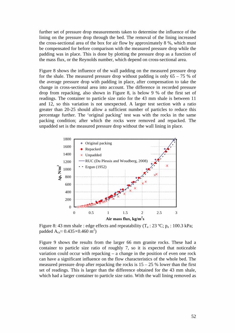
52

further set of pressure drop measurements taken to determine the influence of the lining on the pressure drop through the bed. The removal of the lining increased the cross-sectional area of the box for air flow by approximately 8 %, which must be compensated for before comparison with the measured pressure drop while the padding was in place. This is done by plotting the pressure drop as a function of the mass flux, or the Reynolds number, which depend on cross-sectional area. Figure 8 shows the influence of the wall padding on the measured pressure drop for the shale. The measured pressure drop without padding is only 65 – 75 % of the average pressure drop with padding in place, after compensation to take the change in cross-sectional area into account. The difference in recorded pressure drop from repacking, also shown in Figure 8, is below 9 % of the first set of readings. The container to particle size ratio for the 43 mm shale is between 11 and 12, so this variation is not unexpected. A larger test section with a ratio greater than 20-25 should allow a sufficient number of particles to reduce this percentage further. The ‘original packing’ test was with the rocks in the same packing condition; after which the rocks were removed and repacked. The unpadded set is the measured pressure drop without the wall lining in place.

0

200

400

600

800

1000

1200

1400

1600

1800

0 0.5 1 1.5 2 2.5 3

Air mass flux, kg/m2s

∆p,

N/m

2

Original packing

Repacked

Unpadded

RUC (Du Plessis and Woudberg, 2008)

Ergun (1952)

Figure 8: 43 mm shale : edge effects and repeatability (Ta : 23 ºC; pa : 100.3 kPa; padded Acs≈ 0.435×0.460 m2) Figure 9 shows the results from the larger 66 mm granite rocks. These had a container to particle size ratio of roughly 7, so it is expected that noticeable variation could occur with repacking – a change in the position of even one rock can have a significant influence on the flow characteristics of the whole bed. The measured pressure drop after repacking the rocks is 15 – 25 % lower than the first set of readings. This is larger than the difference obtained for the 43 mm shale, which had a larger container to particle size ratio. With the wall lining removed as

53

before, the recorded pressure drop was 35 – 45 % of the average drop with padding in place. It is expected that the padding would make a bigger difference with larger stones, since there are larger gaps between the stones and the walls with large stones than with small stones.

0

200

400

600

800

1000

1200

1400

1600

1800

0 0.5 1 1.5 2 2.5 3 3.5 4

Air mass flux, kg/m2s

∆p,

N/m

2

Original packing

Repacked

Unpadded

RUC (Du Plessis and Woudberg, 2008)

Ergun (1952)

Figure 9: 66 mm granite: edge effects and repeatability (Ta : 24 ºC; pa : 100.4 kPa) Figure 10 shows the pressure drop over the packed bed at lower flow rates. It is plotted in terms of the inverse of dimensionless pressure drop and the particle Reynolds number. This figure shows mass fluxes between 0 and 2.5 kg/m2s. The difference between the predicted pressure drop and the measured pressure drop where Rep < 3500, not visible in Figure 8 or Figure 9, is more easily seen in the dimensionless format. The RUC and Ergun pressure drop predictions tends to be below the measured pressure drop.

0

0.0005

0.001

0.0015

0.002

0.0025

0 1000 2000 3000 4000 5000 6000Rep

1/K

= 0

.5ρ

fvs2 /∆

p

Measured: originalMeasured: repackedRUC (Du Plessis and Woudberg, 2008)Ergun (1952)

Figure 10: 43 mm shale pressure drop detail

54

The dimensionless pressure drop is influenced by the uncertainty of the mass flow and area measurement in addition to the test section pressure drop measurement. For the shale the uncertainty is greater than 10-15 % at mass fluxes lower than 0.2 kg/m2s (Rep < 500). Where Rep ≤ 3000, the difference between the predicted pressure drop and the measured pressure drop is between 15 % and 35 % (40 % for Ergun) of the measured pressure drop. Above Rep ≈ 3500 (vs ≈ 1.4 m/s) this gap narrows until Rep ≈ 6000, where the predicted pressure may rise above the measured pressure. Figure 11 shows this pattern also occurred with the dolerite and granite rock.

0

0.0005

0.001

0.0015

0.002

0.0025

0.003

0.0035

0.004

0 1000 2000 3000 4000 5000 6000 7000Rep

1/K

=0.

5ρfv

s2 /∆p

Measured: 42 mm dolerite (both packings)Dolerite RUC (Du Plessis and Woudberg, 2008)43 mm shale (both packings)Shale RUC66 mm granite (repacked)Granite RUC

Figure 11: RUC model comparison with measured pressure drop Wen and Ding (2006) measured the pressure drop over a heated cylindrical packed bed of 5 mm spheres. They found that the Ergun equation underestimated pressure drop in a similar Rep range. They suggest that the underestimate of pressure drop at low Reynolds numbers may be due to edge effects and consequent void variation near the walls of the bed, or temperature change of the air through the bed as the air is heated or cooled. However, the difference at lower Rep may also be a consequence of the early onset of turbulence, which will increase the pressure drop through the bed. The shale, although smooth, was generally in the form of flat wide particles, while the granite, although more spherical, was extremely rough. This may have caused higher turbulence and pressure drop through the packed bed. It is not certain whether form drag or surface friction contributes most to the pressure drop in this region. The measured pressure drop over all three sets of rocks is shown in Figure 12 and compared with the correlation of Singh et al. (2006). The only input parameter not known - the sphericity of the rocks – was estimated based on the fit of the correlation, so these plots should be considered best fit lines for the measured

55

data. All three lines are able to fit the measured data with a sphericity of the order of 0.55. The correlation of Singh et al. is dependent on the 1.8th power of the flow speed through the medium.

0

0.0005

0.001

0.0015

0.002

0.0025

0.003

0.0035

0 1000 2000 3000 4000 5000 6000 7000Rep

1/K

=0.

5ρfv

s2 /∆p

Measured: 42 mm dolerite (both packings)43 mm shale (both packings)66 mm granite (repacked)42 mm: Singh et al. (2006); sphericity fit: 0.55566 mm: Singh; sphericity 0.5443 mm: Singh; sphericity 0.54

Figure 12: Comparison with correlation of Singh et al. (2006) Figure 13 shows a comparison of the RUC model against a trendline plotted from the measured data, which shows how the weighted cube length allows for a closer correlation over the full range of pressures. The RUC model was examined with the weighted and unweighted diameters, and was found to follow the measured data less closely over the whole range with the unweighted cubic length. However, a packed bed will probably be used at mass fluxes less than about 1 kg/m2s, so it is more important to predict the pressure drop at low mass fluxes.

0

500

1000

1500

2000

2500

3000

0 0.5 1 1.5 2 2.5 3 3.5Air mass flux, kg/m2s

∆p,

N/m

2

Measured (trendline)

RUC (weighted size)

RUC (unweighted size)

Figure 13: Comparison of particle dimension definition (shale; Ta : 23 ºC; pa : 100.3 kPa)

56

6.3.3 Best fit present method Figure 14 shows the values calculated for c2, defined in equation (3.23), from the Namibian shale pressure drop measurements for different friction factor approximations (values of z). The flow behaviour appears to be turbulent, with friction factors larger than those predicted by Blasius for a smooth pipe, but smaller than those occurring at high Reynolds numbers where f becomes constant. For the shale, a best-fit value of z = -0.21 was found to give an approximately constant value for c2 of 0.74 (c = 10.8). An average value of c2 (0.63) based on the Blasius equation was used to calculate an equivalent Blasius value of c of 14.7. This may be compared with the Blasius value of c for smooth pipes of 0.316.

0

0.5

1

1.5

2

2.5

3

0 500 1000 1500 2000 2500 3000 3500Re

c 2: t

urbu

lent

0

0.01

0.02

0.03

0.04

0.05

0.06

0.07

0.08

0.09

c 2: l

amin

ar

Best fit: z = -0.21Blasius: z = -0.25High Reynolds number: z = 0Laminar flow (secondary axis)

Figure 14: c2 as a function of pore Reynolds number (43 mm shale, repacked) Figure 15 shows a similar pattern for the 66 mm granite, although the friction appears to have been closer to a constant value, with the best fit obtained from z = -0.12. The flow regime again appears to be between Blasius and constant friction factor high Reynolds flow.

0

0.2

0.4

0.6

0.8

1

1.2

0 1000 2000 3000 4000 5000 6000Re

c 2: t

urbu

lent

0

0.01

0.02

0.03

0.04

0.05

0.06

c 2: l

amin

ar

Best fit z = -0.12Blasius z = -0.25High Reynolds number z = 0Laminar flow (secondary axis)

Figure 15: c2 as a function of pore Reynolds number (66 mm granite, repacked)

57

Table 6 summarises the values of c and c2 for the three rock types tested. Table 6: Best fit values of c and c2

Rock z (best fit) c2 c z (Blasius) c2 c 42 mm dolerite -0.18 0.79 8.38 -0.25 0.59 14.3 43 mm shale -0.21 0.74 10.8 -0.25 0.63 14.7 66 mm granite -0.12 0.56 4.9 -0.25 0.34 14.2 Figure 16 shows the inverse of dimensionless measured pressure drop over the bed, for the 43 mm shale, as a function of particle Reynolds number. The Blasius fit (with the measured average value of c2) and the value of z that gave the most constant value of c2 are both plotted. A line showing a possible laminar pressure drop profile - which assumes that the lowest Rep data point measured was close to a transition to laminar flow behaviour - is also plotted. Figure 17 and Figure 18 show the best fit results for the dolerite and granite, which show a similar trend to the shale.

0

0.0005

0.001

0.0015

0.002

0.0025

0 1000 2000 3000 4000 5000 6000 7000Rep

1/K

= 0

.5ρ

fvs2 /∆

p

Measured 43 mm shale (original packing)

Measured (repacked)

Friction factor fit: z = - 0.21

Friction factor fit: Blasius (z = - 0.25)

Friction factor fit: laminar z = -1

Figure 16: 43 mm shale – present method

0

0.0005

0.001

0.0015

0.002

0.0025

0 1000 2000 3000 4000 5000 6000 7000Rep

1/K

=0.

5ρfv

s2 /∆p

Measured: 42 mm dolerite (original packing)

Measured (repacked)

Friction factor fit: z = - 0.18

Friction factor fit: Blasius (z = - 0.25)

Figure 17: 42 mm dolerite – present method

58

0

0.0005

0.001

0.0015

0.002

0.0025

0.003

0.0035

0.004

0 2000 4000 6000 8000 10000Rep

1/K

= 0

.5ρ

fvs2 /∆

p

Measured: 66 mm granite (repacked)

Friction factor fit: z = - 0.12

Friction factor fit: Blasius (z= - 0.25)

Figure 18: 66 mm granite (repacked) – present method For all three sets of tests, the flow regime and friction factor of the bed appears to be between high Reynolds number constant friction factor (z = 0), and Blasius friction (z = -0.25). This suggests that the flow in the bed may be turbulent. The larger, more spherical 66 mm stones, rough on the outside, appear to be close to an almost constant friction factor, while the smaller, smooth but more irregularly shaped 43 mm stones are in the Blasius friction region. For all three tests, the best fit lines show a pressure drop dependence on a power of the flow speed of approximately 1.8. The equation of Singh et al. (2006) is also dependent on the 1.8th power of the superficial flow speed. This suggests that the flow is more turbulent than expected. If the flow is turbulent, then according to equations (3.25) and (3.26), the assumption of an average fluid temperature over the packed bed will be more accurate than for laminar flow.

6.3.4 Comparison with a packed bed of spheres 1200 golf balls, with a void fraction of 0.376 (±0.008), were placed in the test section and the pressure drop measured to show how the Ergun, RUC and Singh et al. equations predict pressure drop for spheres, shown in Figure 19. The particle dimension used in the equations is the actual diameter of the golf balls, 42.6 mm. The RUC and Ergun equations over-predict the pressure drop for Rep > 1000. This is different to the results obtained from the rocks, where the Ergun and RUC model under-predicted the pressure drop at low Rep. The correlation of Singh et al. (2006) predictions are within 8 % of the measured pressure drop. Using the particle sphericity to take the particle shape into account appears to improve the pressure drop estimate and the range of applicability of the Singh et al. correlation.

59

0

0.0005

0.001

0.0015

0.002

0.0025

0.003

0.0035

0 1000 2000 3000 4000 5000 6000 7000Rep

1/K

=0.

5ρfv

s2 /∆p

MeasuredRUC (Du Plessis and Woudberg, 2008)Ergun (1952)Singh et al. (2006) sphericity 1

Figure 19: Comparison with a bed of 42.6 mm spheres (golf balls) In this instance again, the pressure drop appears to be dependent on the 1.8th power of the flow speed, or the friction factor on the flow speed to the power of -0.2. Kays and London (1984) present data showing the friction factor of a packed bed of spheres which also shows a dependence on the flow speed to the power of approximately -0.2. The friction factor data of Kays and London is shown in Figure 20.

0.1

1

100 1000 10000 100000ReK

f K

Kays and London data

Figure 20: Kays and London (1984) friction factor for a bed of spheres, ε ≈ 0.38 Kröger (2004) lists several correlations for predicting the pressure drop over heat exchanger bundles, somewhat similar in principle to packed beds. The correlations show friction factor dependence on powers of the flow speed between -0.2 and -0.316. One of these correlations, by Ganguli et al. (1985), has a term

fK=1.43 ReK-0.15

60

proportional to the flow speed to the power -1 – for the laminar region – and a term proportional to the flow speed to the power -0.2. The Ergun and RUC equations only have friction factor terms dependent on a flow speed power of -1 and 0, which is probably the reason that they do not predict the higher measured pressure drop in the region where Rep < 3500. Figure 21 shows the separate components of the Ergun equation: the laminar term, proportional to 1/Rep, and the fully turbulent term, which is constant. At Rep > 5000 the dimensionless pressure drop approaches that of fully turbulent flow, where the friction factor is constant. At lower flow rates, the laminar friction term drops quickly, which results in an under-prediction of the pressure drop.

0

200

400

600

800

1000

1200

0 1000 2000 3000 4000 5000 6000Rep

K=∆

p/0.

5ρfv

s2

Ergun: turbulent termErgun: laminar termErgun: sum of laminar and turbulentSingh et al (2006) fit: sphericity 0.54Measured

Figure 21: Components of the Ergun equation compared with the correlation of Singh et al. and measurements from the repacked shale If the turbulent term in the Ergun equation is altered so that the pressure drop is dependent on the 1.8th power of the flow speed – the friction factor is proportional to the flow speed to the power -0.2 – and the constant of the turbulent term is altered (reduced by a factor of 10 for this data), it is possible to get it to fit the measured pressure drop and the correlation of Singh et al. This is shown in Figure 22.

61

0

200

400

600

800

1000

1200

0 1000 2000 3000 4000 5000 6000Rep

K=∆

p/0.

5ρfv

s2

Ergun: turbulent termErgun: laminar termErgun: sum of laminar and turbulentSingh et al (2006) fit: sphericity 0.54MeasuredErgun: altered turbulent termErgun: sum of laminar and altered turbulent

Figure 22: Altered turbulent term in the Ergun equation

6.4 Thermal characteristics In this section the measured fluid temperatures at the middle and exit of the rock bed are compared with the temperatures predicted by the E-NTU method of Hughes (1975), described in 4.3.2. The volume weighted mean cube size was used for all predictions. The rock thermal conductivities used for the conductivity correlation of Jeffreson are shown in Table 7, and are based on the values from literature given in Table 1 and Table 2. The lowest expected values are used, and a sensitivity analysis (see Figure 29) was completed to show the influence of the thermal conductivity. Table 7: Rock thermal conductivity for numerical analysis

Rock ks, W/mK Shale 2 Dolerite 3 Granite 3

Figure 23 and Figure 24 show the mid-bed and bed outlet air temperature respectively as a function of time for different mass fluxes. Both figures also show the air inlet temperature to the bed. The general trend of the E-NTU prediction is similar to that of the measured results. The theory over-predicts the air temperature during the initial minutes of charging. This may be due to the thermal capacity of the actual test box. The GLE based on the Ergun equation may tend to under-predict the heat transfer, because the measured pressure drop across the bed is larger than the predicted pressure drop – possibly as a result of higher than expected turbulence from the irregularly shaped rocks.

62

20

25

30

35

40

45

50

55

60

65

70

0 20 40 60 80 100 120Time, min

Tf,

ºC

0.297 kg/m²s mid-bed0.467 kg/m²s mid-bed0.842 kg/m²s mid-bed0.297 kg/m²s Martin xf=0.1970.467 kg/m²s Martin xf=0.1970.842 kg/m²s Martin xf=0.1970.297 kg/m²s inlet0.467 kg/m²s inlet0.842 kg/m²s inlet0.297 kg/m²s Martin xf=0.450.467 kg/m²s Martin xf=0.450.842 kg/m²s Martin xf=0.45

Figure 23: Mid bed fluid temperatures: predicted and measured (shale, Martin/GLE heat transfer correlation and Hughes E-NTU method) Figure 24 shows that the final air temperature measured at the exit of the bed does not reach the temperature of the air at the bed entrance. This is probably due to thermal losses from the fluid to the test section and environment – which should be more significant when low flow rates are tested, since the incoming air is only able to supply a limited amount of energy. However, the final temperature difference recorded between ingoing air and outlet air was between 1 - 2 ºC for 0.297, 0.467, and 0.842 kg/m2s, so this may not be the cause, particularly since the temperature difference between the mid-bed measurement and the inlet temperature (Figure 23) at the end of charging is negligible.

20

25

30

35

40

45

50

55

60

65

70

0 20 40 60 80 100 120Time, min

Tf,

ºC

0.297 kg/m²s outlet0.467 kg/m²s outlet0.842 kg/m²s outlet0.297 kg/m²s Martin xf=0.1970.467 kg/m²s Martin xf=0.1970.842 kg/m²s Martin xf=0.1970.297 kg/m²s inlet0.467 kg/m²s inlet0.842 kg/m²s inlet0.297 kg/m²s Martin xf=0.450.467 kg/m²s Martin xf=0.450.842 kg/m²s Martin xf=0.45

Figure 24: Bed exit fluid temperatures: predicted and measured (shale, Martin/GLE heat transfer correlation and Hughes E-NTU method)

63

A comparison between calculated and measured mid-bed and exit air temperatures during discharge is shown in Figure 25. There was a time interval between the completion of charging and initiation of discharging of 10 minutes. When the wind tunnel was turned on to discharge, it took several minutes for the outlet thermocouples to heat up, which is why there is a discrepancy between the predicted and measured outlet air temperature during the initial 5 – 7 minutes. The experimental apparatus did not allow the packed bed to be turned around before discharge, so the flow direction through the bed remained the same. The analytical model took this into account.

20

25

30

35

40

45

50

55

60

65

70

0 10 20 30 40 50 60Time, min

Tf,

ºC

Measured (inlet)Measured (exit)Measured (mid-bed)Martin GLE, xf=0.45 (mid-bed)Martin GLE, xf=0.45 (exit)

º

Figure 25: 43 mm shale, discharging, 0.0940 kg/s (0.470 kg/m2s) The different heat transfer correlations are compared with each other and a set of measured temperatures in Figure 26. The Martin GLE equation with xf = 0.45 predicts fluid temperatures similar to the equations of Gunn, Aly and El-Sharkawy, and Wakao et al. The only correlation that does not match up with the others is the GLE used with xf = 0.197. The difference between the Martin GLE for xf = 0.197 and the measured results may be because it is based on the Ergun equation, which, as seen from Figure 10, underestimates the pressure drop where Rep < 3500. If the flow is more turbulent than expected at low Rep, it will result in higher heat transfer coefficients, and hence the GLE will underestimate the heat transfer to the solid particles. If the GLE is written in terms of the measured pressure drop, by means of a best fit form of equation (3.23), it will be based on the actual measured pressure drop through the packed bed. It may be seen in Figure 23 - Figure 26 that xf = 0.45 in the Martin GLE gives temperature prediction similar to the other heat transfer correlations used and the measured data. Singh et al (2006) found that if the sphericity of the particles is close to 0.55, the Nusselt numbers will be similar to those for spheres (ψ = 1).

64

Since the pressure drop results for the Singh pressure drop correlation best match the measured pressure drop for a sphericity of 0.5–0.6, it appears that the rocks tested give rise to flow patterns similar to particles of sphericity 0.5–0.6. Thus the heat transfer coefficient may be similar to that of spheres, not cubes, and the GLE will give closer predictions with xf = 0.45 instead of 0.197.

20

25

30

35

40

45

50

55

60

65

70

0 20 40 60 80 100 120Time, min

Tf,

ºC

Inlet (measured)

Mid-bed (measured)

Outlet (measured)

Gunn / Shen and Wakao

Aly and El-Sharkawy

Wakao et al.

Martin GLE, xf=0.197

Martin GLE, xf=0.45

Figure 26: Comparison of heat transfer coefficient correlations (shale, 0.297 kg/m2s) A comparison between predicted temperatures from the GLE, based on the Ergun equation and the measured pressure drop, is shown in Figure 27. The difference in predicted temperatures based on the Ergun equation and the measured pressure drop is less than 1.5 ºC.

25

30

35

40

45

50

55

60

0 10 20 30 40 50 60Time, min

Tf,

ºC

Martin GLE, z = - 0.25, xf=0.45

Martin GLE, Ergun, xf=0.45

Martin GLE, z = - 0.25, xf=0.197

Martin GLE, Ergun, xf=0.197

Figure 27: Comparison of Martin GLE air outlet temperature predictions for Ergun predicted and measured pressure drop (43 mm shale, 0.297 kg/m2s)

65

The influence of the particle conductivity depends on the heating or cooling rate of the particle. Figure 28 shows the temperature change for a single 40 mm sphere (ks = 2 W/mK) initially at 70 ºC that is placed in a stream of air at 25 ºC and allowed to cool at a Biot number of 0.4. The maximum difference between the sphere surface temperature calculated from the lumped capacity method, and the Biot–Fourier number method (see Mills, 1999) is less than 3 ºC. However, this is for one sphere only, and does not imply that there will be equally small temperature differences over a packed bed of several particles. The Biot-Fourier method cannot be used for packed beds with the Hughes E-NTU method, so it is replaced by the correlations of Sagara and Nakahara (1991) or Jeffreson (1972) for the calculation of bed temperatures in this study.

20

30

40

50

60

70

0 5 10 15 20 25 30 35Time, min

Ts,

ºC

Biot modified centre temperatureLumped capacitance modelBiot modified surface temperature

Figure 28: Temperature of a sphere cooled in a fluid at 25 ºC (BiD ≈ 0.4) The effect of the rock thermal conductivity on the predicted temperatures in the packed bed is shown in Figure 29, for BiD ≈ 0.5.

15

20

25

30

35

40

45

0 5 10 15 20 25 30Time, min

Tf,

ºC

Jeffreson, ks=3 W/mK Sagara & Nakahara, ks=3 W/mKJeffreson, ks=7 W/mK Sagara & Nakahara, ks=7 W/mK

Figure 29: Effect of thermal conductivity on predicted fluid temperatures (dolerite, 0.365 kg/m2s, Martin GLE, xf=0.45)

66

The NTU adjustments of Jeffreson (1972) – equation (4.27) – and Sagara and Nakahara (1991) – equation (4.9) – were used to generate Figure 29. The maximum difference is less than 2 ºC between predictions with a thermal conductivity of 3 W/mK and 7 W/mK. This suggests that, for the given conditions, measuring the exact value of the thermal conductivity is not critical to correctly simulate the thermal behaviour of the bed, provided an approximate value from literature may be used. For these conditions, the correlations of Sagara and Nakahara and Jeffreson give similar results for a given conductivity. Predicted and measured temperatures for the air in the 66 mm granite and the 42 mm dolerite packed bed are shown in Figure 30 and Figure 31. The results are similar to those obtained for the shale – including a difference of 2 – 3 ºC between the fluid inlet and outlet temperature at the end of the charging process. It is probable that this is due to thermal losses to the test section walls. Apart from this, it can be seen that the E-NTU method predicts the trend of the air temperature passing through the packed bed.

20

25

30

35

40

45

50

55

60

65

70

0 20 40 60 80 100 120 140 160Time, min

Tf,

ºC

Inlet (measured)Mid-bed (measured)Exit (measured)Martin GLE, xf = 0.45, mid-bedMartin GLE, xf = 0.45, exit

Figure 30: 66 mm granite air temperatures (charging, 0.321 kg/m2s)

67

10

20

30

40

50

60

70

80

0 20 40 60 80 100 120 140Time, min

Tf,

ºC

Inlet (measured)Mid-bed (measured)Exit (measured)Martin GLE, xf=0.45, mid-bedMartin GLE, xf=0.45, exit

Figure 31: 42 mm dolerite air temperatures (charging, 0.365 kg/m2s)

6.5 Rock thermal cycling tests at temperatures above 500 ºC The sandstone heated in the packed bed was heated to 70 ºC. Even at this relatively low temperature, a fine powder formed on the surface of the rocks and blew into the tunnel. This implies that sandstone is unsuitable for use in thermal storage. The shale was thermally cycled between room temperature and about 200 ºC in an oven. Some of the samples formed hairline cracks after 15 cycles. Three samples each of shale, granite, dolerite, slag and veined (impure) quartz were thermally cycled at temperatures between room temperature (≈ 21 ºC) and 510 ºC. For the first ten cycles, the samples were heated to 510 ºC by placing them in the oven before turning it on, and allowing them to warm with the oven. The oven took approximately 1 hour to heat up to 510 ºC. After the first ten cycles the oven was pre-heated to 510 ºC, and the samples were placed in the oven and removed at intervals of about 45 - 50 minutes. This process was continued for over a hundred cycles. The rate at which the samples are heated and cooled will have an influence on the number of cycles rocks can withstand. The samples in the oven are heated by natural convection, radiation from the oven walls, and conduction from contact with the oven walls. The equivalent heat transfer coefficient for radiation and convection heat transfer to the rock, when the rock is at 50 ºC and the oven at 510 ºC, is of the order of 20 - 30 W/m2K (see Appendix I), if conduction to the rock from the oven is considered to be negligible in comparison with radiation and convection heat transfer. By way of comparison, the heat transfer coefficient in a packed bed with forced convection, at mass fluxes of about 0.2 kg/m2s, is of the order of approximately

68

20 - 40 W/m2K (see Appendix I), depending on particle size. The rate at which the rocks in a packed bed will heat or cool may be higher than the rate at which the samples in the oven are heated, so the number of cycles they last in the oven is not an exact indication of the number of cycles they can last. On the other hand, the samples in the oven are handled all the time, and are subjected to shock changes in temperature when they are placed in the oven or removed, so it is probably a fair indication. The shale fractured severely in the first two thermal cycles – as shown in Figure 32. One quartz sample cracked along a seam of impurity during the first 5 cycles and separated into two parts within the first 10. It fragmented completely within 30 cycles, shown in Figure 34. A second quartz sample with fewer impurities and veins broke in two after 60 cycles. The slag became brittle and friable and pieces broke off when the samples were removed from the oven. In 60 cycles both samples of slag broke into several parts, shown in Figure 33. One dolerite sample fractured the first time it was placed into the pre-heated oven; although it did not fracture when heated up slowly with the oven for the first ten cycles. The fractured sample is shown in Figure 35. If the dolerite tends to shatter like this when suddenly heated, it has implications for the maximum rate of charging of a packed bed, and the initial air inlet temperature at the onset of charging. The other dolerite samples did not fracture noticeably in 125 cycles, although they started showing hairline cracks after about 60 cycles, shown in Figure 36. The granite samples did not break apart or show any noticeable cracks after 125 cycles. Some very small fragment broke off the surface of one of the samples. A granite sample is shown in Figure 37.

69

Figure 32: Structural failure of shale above 500 ºC

Figure 33: Fragmented slag sample after 60 cycles

Figure 34: Fragmented quartz sample after 30 cycles

Figure 35: Dolerite explosive failure during first heating

Figure 36: Hairline fracture of dolerite after 110 cycles

Figure 37: Granite after 110 cycles

70

7 Large packed beds Some possible configurations of large beds are examined in this chapter, along with approximate bed sizes for chosen power outputs.

7.1 Geometry As seen in the literature, in order to reduce the effects of natural convection (Sanderson and Cunningham, 1995b), and obtain a higher efficiency (Adebiyi et al., 1998), a packed bed should be charged by allowing the hot air in at the top of the bed and removing the cooled air from the bottom of the bed and reversing this process for discharge. The slag bed of Curto and Stern (1980) was designed in the shape of a cone, with the hot air for charging the bed introduced at the top and several outlets at the base of the cone. This has the disadvantage that the fluid flow speed changes through the bed, and will be higher near the inlet where the cross-sectional area is small. This will result in a larger pressure drop near the top of the bed. There might be difficulties with flow distribution over the entire cross-section of the bed, which would result in part of it not storing heat.

Figure 38: Slag packed in a conical mound as in Curto and Stern (1980) Turner (1980) suggests excavating a trench in the ground, placing air headers at the bottom of the trench, filling it with rock, and placing air headers at the top. Sanderson and Cunningham (1995a,b) recommend the use of flow distributors at the inlet and outlet of packed beds. The simplest packed bed geometry is probably that shown in Figure 39. Ducts at the top and bottom of the bed carry the air into and out of the bed.

Figure 39: Cross-sectional bed layout with charging air-flow direction

71

Additional ducts might be placed between the top and bottom of the bed in order to allow sections of the bed to be charged at a time, as shown in Figure 40. This would allow a reduction in pressure drop and pumping power requirements.

Figure 40: Additional ducts for charging sections of the bed This layout has the disadvantage that the top and sides of the bed are at elevated temperatures, which might result in significant losses to the environment unless they are well insulated. Figure 41 shows a layout which may allow for less high temperature surface in contact with the surroundings. The segments will have to be divided horizontally to reduce natural convection effects.

Figure 41: Cross-section of alternative horizontal bed layout Another layout for reducing the thermal losses is shown in Figure 42. The air will be cooled as it passes through the bed from the centre, so the outer edges of the bed are not at temperatures higher than the environment. A disadvantage of this is that the upper half of the bed will be charged from the bottom up, which may result in natural convection destratifying the bed.

Figure 42: Cross-sectional area of bed to reduce thermal losses

7.2 Temperature and pressure drop predictions for large beds This section discusses the assumptions and calculation methods used to simulate and predict the thermal and pressure drop characteristics of large packed beds of

72

rock, intended for use in solar power plants. The predicted thermal performance and pressure drop characteristics are presented for packed beds of 50, 100 and 200 mm rocks, sized to store the thermal energy in the exhaust of a gas turbine which runs at design capacity for 8 hours. If a packed bed is to be used in the SUNSPOT concept, it may be required to store approximately 8 hours of thermal energy from the gas turbine exhaust. For a 100 MWe gas turbine, the charging of the bed is simulated for an assumed turbine exhaust gas temperature of 528 ºC and a mass flow rate of 300 kg/s. This mass flow rate is linearly scaled from the Siemens SGT-700 gas turbine (Siemens, 2009). In 8 hours, the total heat energy in the exhaust is about 1200 MWhth. It is assumed that the exhaust mass flow rate and temperature are constant for the full 8 hours. In other words, if the available solar power is insufficient to power the gas turbine, a combustion chamber is used either to keep the gas turbine running at constant (design) mass flow rate and outlet temperature, or to provide hot air directly to charge the packed bed at the same mass flow rate and temperature which would be available if the gas turbine were running under design conditions. The rock beds of different rock sizes are sized to store all the heat from a mass flow of 300 kg/s at a temperature of 528 ºC. The exhaust air from the bed during charging does not rise more than 1 ºC above the ambient temperature, assumed to be 25 ºC. The air inlet temperature to the bed during discharging is assumed to be 25 ºC. In future the possibility of feeding the exhaust air, at higher temperature, from the steam boiler back into the packed bed should also be examined. When the beds are discharged, the bed discharge is halted as soon as the air outlet temperature drops below the chosen temperature limit, chosen to be 475 ºC. The packed bed is then re-charged for 8 hours and discharged again. The time before the bed outlet temperature drops below the limit during discharing is the total time for which the steam turbine is assumed to generate electricity from the stored heat. The input parameters for the simulations are listed in Table 8. The properties of the granite were used, with a slightly lower specific heat capacity of 840 J/kgK instead of 845 J/kgK, since this matches the average value for rock given by Dincer et al (1997). Table 8: Values used for calculating large bed performance cs 840 J/kgK Initial bed temperature 25 ºC ks 3 W/mK Tf (discharge inlet temp) 25 ºC ρs 2893 kg/m3 Gas turbine outlet temperature 528 ºC ε 0.38 ψ 0.54

fm� (charging) 300 kg/s fm� (discharging) 224 kg/s

Acs 40 × 40 m2 Tenv (ambient air temperature) 25 ºC The average specific heat capacity of air between 528 ºC and 25 ºC is taken as 1028 J/kgK, from Mills (1999). The total heat Qtot entering the packed bed in 8 hours of charging, calculated from these input parameters, is 4.5 × 1012 J. The

73

initial bed temperature before charging begins, the air inlet temperature to the bed during discharging, and the ambient temperature are all assumed to be 25 ºC. The atmospheric pressure is assumed to be 100 kPa. The calculation method used for simulating the large bed characteristics is the same as that used to predict the characteristics of the test section used for the experimental tests (Chapter 6). The bed was divided into segments 20 – 58 mm in length (depending on bed length) and the Hughes E-NTU method (equations (4.24) and (4.26)), in conjunction with the Martin GLE equation, (4.10) (xf = 0.45), was used to simulate the temperature profile through the packed bed. The particle conductivity NTU adjustment of Sagara and Nakahara (1991) was used to include particle internal thermal resistance effects. The temperature profile of the bed at the end of the charging cycles was used as the temperature profile at the start of the discharging process. The pressure drop over the bed is determined by calculating the pressure drop over each bed segment, with the correlation of Singh et al. (2006) – equation (3.20) – and the air properties inherent to that segment, and summing the individual segment pressure drops together to obtain the total pressure drop. The bed discharge temperature characteristics below exclude possible losses to the environment, poor flow distribution effects, and radiation and conductivity diffusion effects through the bed. Diffusion may become significant, especially if the heat is stored for several hours before use. Further work is required to determine the importance of these effects where heat is to be stored for relatively lengthy time periods. The air mass fluxes through the bed during charging and discharging were chosen below 0.2 kg/m2s in order to reduce pressure drop over the bed. Bed performance was simulated for 0.05, 0.1 and 0.2 m rock sizes, greater than the minimum of 13 mm recommended by Sanderson and Cunningham (1995a,b) but less than one thirtieth of the bed hydraulic diameter and length (Torab and Beasley, 1987). The cross-sectional area of the bed was kept constant, while the length of the bed was allowed to vary to determine the required bed volume for different particle sizes. Figure 43 and Figure 44 show air outlet temperature profiles for rock beds of different particle sizes, sized to store all the heat from a mass flow of 300 kg/s at a temperature of 528 ºC. The discharge temperatures from a packed bed of 200 mm rocks during the first four charge-discharge cycles of the bed are shown in Figure 43. The packed bed does not charge completely during the first charging period of 8 hours, and is not even able to supply air at temperatures above 475 ºC for an hour. However, after the next charging cycle, the bed is able provide air above 475 ºC for over 8 hours. The bed reaches its maximum capacity after the third charging session, and after this is able to supply air for 10 hours.

74

Figure 44 compares the outlet temperatures from packed beds of the different rock sizes. It can be seen that smaller rocks allow for a constant air outlet temperature from the bed for longer than large rocks allow. The low volumetric surface area of large rocks reduces the heat transfer from the rock to the air. However, the smaller rocks result in a larger pressure drop over the packed bed, as seen in Figure 45.

460

470

480

490

500

510

520

530

540

0 1 2 3 4 5 6 7 8 9 10 11Time, hours

Tf,

ºC

Discharge 1

Discharge 2

Discharge 3

Discharge 4

Figure 43: Air discharge temperatures for 0.2 m rock (L = 23 m; G = 0.14 kg/m2s)

470

480

490

500

510

520

530

540

0 1 2 3 4 5 6 7 8 9 10 11 12 13Time, hours

Tf,

ºC

0.05 m discharge 10.05 m discharge 40.10 m discharge 10.10 m discharge 40.20 m discharge 10.20 m discharge 4

Figure 44: Comparison of rock size effect on air outlet temperature during discharge of packed bed at 0.14 kg/m2s (224 kg/s, air inlet temperature 25 ºC) The dimensions of the beds for the different rock sizes are summarised in Table 9. The ratio of the increase in availability (from equation (2.1)) in the bed with every charge to the total heat stored in 8 hours during charging is also shown. It can be seen that the small rocks allow for more efficient storage of exergy – useful

75

energy – than large rocks. However, these figures do not include pumping energy requirements, which may be larger for small particles than large particles, even if the bed can be charged in segments. The charging mass flux for a cross-sectional area of 1600 m2 is 0.1875 kg/m2s. Equation (2.2) gives 0005.0=G , which is smaller than the value of 0.05 recommended by Krane (1987). This means the bed is larger than he considers necessary, and that the mass flux is sufficiently low to avoid large pressure drop pumping requirements. Table 9: Packed bed characteristics (Acs = 40 × 40 m2)

D, m L, m Vbed, m3 Rock mass, kg ∆φ /Qtot, %

0.05 10.5 17 × 103 50 × 106 29 0.1 14.5 24 × 103 68 × 106 23 0.2 23 37 × 103 106 × 106 16

The discharge of the bed is based on an assumed average steam cycle efficiency of η = 30 %, which is similar to efficiencies found in literature (for example, Fricker, 2004). The total heat energy flow rate available in the bed outlet air for the steam cycle is estimated from f pf fQ m c T= ∆� � where the change in air

temperature is the difference between the average outlet temperature (≈ 500 ºC) and the ambient temperature. The electrical power output from the steam cycle is roughly estimated from eP Qη= � .

The discharge air flow of 0.14 kg/m2s, (224 kg/s for 40 × 40 m2) should be more than sufficient to supply a 25 - 30 MWe steam turbine for 10 hours (see Appendix I), generating 250 – 300 MWhe, depending on the ambient temperature. The electrical energy generated from the storage can be compared with the figure for the Andasol molten salt storage (section 2.4) – 375 MWhe for a total salt storage tank volume of about 30 × 103 m3. If the bed of 0.05 m rocks is only able to allow the generation of 250 MWhe, and is linearly scaled to the same output as the Andasol salt storage generation capacity of 375 MWhe, it has a volume of 26 × 103 m3. The bed of 0.1 m rocks would need to be about 36 × 103 m3 in volume. A rock bed with the given properties would require a similar storage volume to existing molten salt storage. It should be remembered that this excludes possible thermal losses. The pressure drop over the packed bed of different rock sizes is shown in Figure 45. These pressure drop curves were calculated with the equation of Singh et al. (2006) and the best fit sphericity of 0.54 that was obtained from the experimental tests. The pressure drops over each segment were calculated with the air properties of the segment. The total pressure drop was calculated by summing the segment pressure drops together. The pressure drop for the initial charge, when the bed is at 25 ºC throughout, is lower than the pressure drop during the second charge of the bed, since the air temperature through the bed is higher after the second charge than the first. As the bed temperature increases during charging, the

76

pressure drop increases, presumably as a consequence of decreasing air density and increased flow speeds.

0

50

100

150

200

250

300

350

400

450

0 1 2 3 4 5 6 7 8Time, hours

∆p,

N/m

2

0.05 m charge 1 0.05 m charge 20.1 m charge 1 0.1 m charge 20.2 m charge 1 0.2 m charge 2

Figure 45: Pressure drop during charging of bed for different rock sizes The pressure drop over the bed increases more in 8 hours of charging for the small rocks than the large rocks. This is because the smaller rock sizes make the pressure drop more sensitive to changes in the air speed through the bed than larger rocks do. However, even the 0.05 m rock bed does not have a bed pressure drop as large as 1.2 × 103 N/m2, which is the figure given by Fricker (2004) – see section 2.4 – for a packed bed supplying heat to a 7 MWe steam cycle. The pressure drop is lower than that recommended by Torab and Beasley (1987) – 0.5 – 1 N/m2/m – so even flow distribution through the bed may be problematic. It may be possible to reduce this by means of air distribution headers at the bed inlet and outlet - further work is required to determine the importance of this. It is assumed that the air density at the fans will be about 1.1 – 1.2 kg/m3. This is possible if the fans are used to draw air through the bed during charging, and the reverse during discharging. The suggestion of Meier et al. (1991) that the pumping power requirement should not be more than 1 – 2 % of the power output from the plant is met even by the 0.05 m rocks, which would require less than 0.5 % of the output from a 25 MWe steam cycle, which the packed bed should be able to drive for at least 10 hours. This figure does however exclude pumping power requirements for air ducts and other sources of pressure drop. Figure 46 shows the temperature profile in the packed bed of 0.05 m rocks at positions along the length of the bed. It can be seen that for the first 3 hours of every charge cycle, the exhaust air could be extracted from the bed three quarters along its length, since the temperature at this point does not rise above 25 ºC until after 3 hours. This would reduce the pressure drop over the bed, and reduce the total pumping power required. Since smaller rocks give sharper temperature

77

waves (higher volumetric heat transfer), it will be possible to charge smaller segments at a time with beds of small rocks than beds of bigger rocks. This possible reduction in pumping power through packed beds may allow the use of smaller particles for a similar total pumping power, but at a higher exergetic efficiency than large particles would give.

0

100

200

300

400

500

600

0 1 2 3 4 5 6 7 8Time, hours

Tf,

ºC

QuarterMid-bedThree quarterExit

Figure 46: Solid temperature profile at different positions in a bed of 0.05 m rocks Average hydraulic pumping power requirements for the beds are given in Table 10. The reduced pumping work for the 0.05 m bed if the air is removed at the three quarter length position for the first 3 hours is also shown – the reduction in pumping energy required is about 7 %. Even with this reduction, however, the ratio of bed availability gained during charging is smaller than those for the larger rocks. This matches the statement of Torab and Beasley (1987) in section 2.2 that the ratio of total availability to total hydraulic pumping energy increases with increasing particle size; and in this case, this is despite the fact that the bed length has also increased. Table 10: Typical bed power and energy requirements for 8 hours charging D, m Pp, W (eqn (3.27)) Wp, J Wp reduced, J ∆φ /Wp 0.05 90 × 103 2.6× 109 2.4 × 109 522 0.1 53 × 103 1.5 × 109 - 670 0.2 35 × 103 1.0 × 109 - 720

The cost of the packed bed, beyond the scope of this study, will be an important parameter in determining an optimum bed and rock size.

78

8 Conclusions and further work required Conclusions from the study are summarised, after which suggestions for further work are made.

8.1 Conclusions from work done The existing pressure drop prediction models are able to predict the general trend of the pressure drop over a packed bed of irregularly shaped rocks up to particle Reynolds numbers of about 7000. However, The RUC model of Du Plessis and Woudberg (2008) predicts pressure drops about 25 - 35 % less than the measured pressure drop at Rep < 3500. The Ergun equation tends to under-predict by up to 30 - 40 %. The pressure drop correlation of Singh et al. (2006) fits the measured pressure drop for all three rock sets for Rep < 4000 for sphericities between 0.54 and 0.56. It predicts the measured pressure drop over a packed bed of spheres to within 8 %. The best fit present method needs further experimental data over a range of sizes to determine if rocks have friction constant values that could be used to predict pressure drop. The dependence of z – if there is – on the rock geometry and size also needs to be found. This method found best fit lines for predicting pressure drop that suggest the pressure drop is proportional to a power of the Reynolds number/superficial speed between 1.79 and 1.89 for the three rock types tested. This is a similar power to that used in the correlation of Singh et al. even though it does not take the particle shape into account. This suggests that the pressure drop in packed beds over a significant range of Reynolds numbers is proportional to the 1.8th power of the Reynolds number/flow speed, which implies that the friction factor is proportional to air speed to the power -0.2. The experimental data given by Kays and London (1984) also follows this trend, as do several correlations for determining the pressure drop across heat exchangers. The Hughes E-NTU method, combined with the heat transfer correlations of Gunn (1978), Wakao et al. (1979), Aly and El-Sharkawy (1990) and Martin (GLE) (2005) estimate the fluid temperature to within 15 % of the temperature drop over the packed bed. The GLE provides heat transfer coefficients similar to the other correlations where xf = 0.45 (spheres), but not for xf = 0.197 (cubes). From the work of Singh et al. (2006) it appears that the Nusselt number of particles with a sphericity of 0.55 is similar to the Nusselt number of a sphere (ψ = 1). Hence for particles of sphericity 0.6 or less the use of xf =0 .45 will probably give more accurate Nusselt number predictions than xf = 0.197.

79

The sandstone and shale rock samples failed structurally at temperatures above 70 and 200 ºC respectively, and are therefore not suitable for use at higher temperatures. Quartz samples with impurities (veins) in them fractured and fell apart within 40 cycles when thermally cycled between 510 ºC and room temperature. Quartz with veins of impurities is not suitable for thermal cycling. Slag samples all broke apart within 60 cycles. Dolerite samples started showing hairline cracks after 60 cycles, but did not break within 125 cycles. However, one dolerite sample cracked significantly the first time it was heated. The granite rocks did not fracture noticeably within 125 cycles. Based on these results, granite, and to a slightly lesser extent dolerite, may be suitable for use in packed bed storage. However, their ability to withstand several thousand thermal stress cycles is still uncertain. The volume of rock beds to store the energy from the exhaust of a 100 MWe gas turbine is estimated to fall in the range of 17 – 37 × 103 m3, depending on the rock size. Such a bed should be able to provide 224 kg/s of air at temperatures above 475 ºC for 10 hours or more after they have been through three charge-discharge cycles. This should be sufficient to provide heat to a 25 – 30 MWe steam turbine for at least 10 hours. When compared to the Andasol molten salt storage on a volumetric basis only, a packed bed of 0.05 m or 0.1 m particles should be able to store the same quantity of heat in a similar volume.

8.2 Recommendations and further work required Further work is needed in the areas discussed below, if the concept of rock storage is to be examined in further detail and accurate sizing and costing of packed beds is to bed done. Pressure drop and thermal tests on larger rock beds with a higher bed to particle size ratio should be completed to confirm that the results obtained are similar to results obtained at low bed to particle size ratios with a lining to reduce channelling; that the analytical model predictions are still correct. This should be done in combination with more accurate void fraction measurements. Further work is needed to examine the influence of particle shape and roughness on the pressure drop, heat transfer and flow regime, particularly in the region where Rep < 4000, where the Ergun and Du Plessis equations generally underestimate the pressure drop for rock beds. Rigorous thermal cycling tests of thousands of cycles are needed to determine longevity of rock or slag and its resistance to cracking, exfoliation or powdering. Further testing on quartz, granites, dolerites and other rocks is needed to determine the effect of particle size and rock composition on their ability to

80

withstand thermal cycling. Examination of the rate at which rocks are heated and cooled and the influences on how easily they crack is needed to determine limitations on the speed of charging and discharging the packed bed. The influence pre-heating and drying has on preventing fracture should also be considered. The airflow distribution in large beds needs to be planned and analysed to determine a means of distributing the air evenly through the bed while minimising pressure drop. The air needs to be transported in some form of channel, duct or canal that will not rust, corrode or fracture at temperatures near 500 ºC. The feasibility of charging segments of a packed bed at a time should also be considered, since this should require less pumping work. The cost of a large bed needs to be estimated and compared with existing storage options to determine its economic feasibility. Aspects such as the environmental friendliness of the rock/slag bed should be considered when comparison is made with molten salt or oil beds. The importance of radiation and conduction heat transfer between particles in the bed and other particles and the fluid in the bed at temperatures above 300 ºC needs to be examined. The effect of radiation on thermal diffusion through a large packed bed over time periods of hours or days should be analysed. Jalalzadeh-Azar et al. (1996) calculated values for L/D that provided a maximum First and Second Law efficiency for their specific conditions. It would be useful to have a parameter including the dimensionless L/D value that could be used to predict maximum second law efficiency of a packed bed. Suggested improvements in the experimental apparatus include the ability to turn the rock bed around for discharge to emulate reversal of flow direction. A door/barrier between the heat exchanger and the packed bed would allow pre-heating of the heat exchanger without pre-heating of the rocks. Since the packed bed would probably be used at Rep <1000, measurement accuracy at low flow rates needs to be improved, to allow measurements to be made. The heat loss to the tunnel walls should be reduced or compensated for in some way.

81

9 References Adebiyi, G. A., Nsofor, E. C., Steele W. G., Jalalzadeh-Azar, A. A., 1998. Parametric study on the operating efficiencies of a packed bed for high-temperature sensible heat storage, ASME Journal of Solar Energy Engineering, 120: 2 – 13 Aly, S. L., El-Sharkawy, A. I., 1990. Effect of storage medium on thermal properties of packed beds, Heat Recovery Systems and CHP, 10.5/6: 509-517 Arndt, J., Bartel, T., Scheuber, E., Schilling, F., 1997. Thermal and rheological properties of granodioritic rocks from the central Andes, North Chile, Tectonophysics, 271: 75-88 Balakrishnan, A. R., Pei, D. C. T., 1979a. Heat transfer in gas-solid packed bed systems: A critical review, Industrial Engineering Chemistry Process Design and Development, 18.1: 30 – 40 Balakrishnan, A. R., Pei, D. C. T., 1979b. Heat transfer in gas-solid packed bed systems: The conduction mode, Industrial Engineering Chemistry Process Design and Development, 18.1: 40 – 46 Balakrishnan, A. R., Pei, D. C. T., 1979c. Heat transfer in gas-solid packed bed systems: The conduction mode, Industrial Engineering Chemistry Process Design and Development, 18.1: 47 – 50 Barreiros, F.M., Ferreira, P.J., Figueiredo, M.M., 1996. Calculating shape factors from particle sizing data, Particle and Particle Systems Characterization, 13: 368 - 373 Bear, J., Bachmat, Y., 1991. Introduction to Modelling of Transport Phenomena in Porous Media. Kluwer Academic Publishers, Netherlands. Beasley and Clark, 1984. Transient response of a packed bed for thermal energy storage, Int Journal of Heat and Mass Transfer, 27.9: 1659 – 1669 Beltagui, S.A., 1983. Optimum design of a packed bed thermal storage system, Alternative Energy, 6.1: 183 – 190 Bennett, C.O., Myers, J.E., 1962. Momentum, Heat and Mass Transfer, McGraw-Hill Book Company, Inc., New York Brittain, H. G., 1995. Physical Characterization of Pharmaceutical Solids, Informa Health Care

82

Chandra, P., Willits, D. H., 1981. Pressure drop and heat transfer characteristics of air-rockbed thermal storage systems, Solar Energy, 27.6: 547 – 553 Curto, P.A, Stern, G., 1980. Thermal storage using slag, Alternative Energy, 3.1: 195 – 208 De Souza-Santos, M. L., 2004. Solid Fuels Combustion and Gasification: Modeling, Simulation and Equipment Operation, Marcel Dekker Inc., New York Diedericks, G.P.J., 1999. Pore-scale modelling of transport phenomena in homogeneous porous media. PhD thesis, Stellenbosch University, Stellenbosch Dincer, I., Dost, S. and Xianguo, L., 1997. Performance of sensible heat storage systems for thermal applications, Int Journal of Energy Research, 21:12 1157 – 1171 Dinter, F., 1992. Thermische Energiespeicher in Solarkraftwerken und ihre Bewertung. Aachen: Verlag Shaker Dixon, A.G., Cresswell, D.L, 1979. Theoretical prediction of effective heat transfer parameters in packed beds, American Institute of Chemical Engineers (AIChE) Journal, 25.4: 663-676 Dullien, F.A.L. 1979. Porous media: fluid transport and pore structure. Academic Press Dullien, F.A.L, 1992. Porous media: fluid transport and pore structure. Second edition, Academic Press [Not read] Duffie, J.A., Beckmann, W.A., 1991. Solar engineering of thermal processes, Second edition, Wiley, New York Du Plessis, J.P., Masliyah, J.H., 1988. Mathematical modeling of flow through consolidated isotropic porous media, Transport in Porous Media, 3: 145-161 Du Plessis, J.P., 1991. Saturated crossflow through a two-dimensional porous medium, Advances in Water Resources, 14.3: 131-137 Du Plessis, J.P., Masliyah, J.H., 1991. Flow through isotropic granular porous media, Transport in Porous Media, 6.3: 207-221 Du Plessis, J.P. 2002. Modelling and industrial application of flow through two-dimensional porous media. MScEng Thesis, Stellenbosch: University of Stellenbosch

83

Du Plessis, J.P., Woudberg, S., 2008. Pore-scale derivation of the Ergun equation to enhance its adaptability and generalisation, Chemical Engineering Science, 63: 2576-2586 Du Plessis, J.P., email correspondence, December (10th – 19th) 2008 Elsayed, M.M., Megahed, I.E., El-Refaee, M.M., 1988. Experimental testing of fluidized bed thermal storage, Solar and Wind technology, 5.1: 15 – 25 [Not read] Energy Solutions Centre, Accessed 5th February 2009 http://www.energysolutionscenter.org/boilerburner/Eff_Improve/Primer/Boiler_Introduction.asp Ergun, S., 1952. Fluid flow through packed columns, Chemical Engineering Progress, 48.2: 89-94 Figliola, R.S., Beasley, D.E., 2006. Theory and Design for Mechanical Measurements, 4th edition, John Wiley and Sons, inc. Pp 307 Fluri, T.P., 2009. Personal communication Fraidenraich, N., Gordon, J.M., Tiba, C., 1992. Optimisation of gas-turbine combined cycles for solar energy and alternative fuel power generation, Solar Energy, 48.5: 301 – 307 Fricker, H.W., 1991. High temperature heat storage using natural rock, Solar Energy Materials, 24: 249 – 254 Fricker, H.W., 2004. Regenerative thermal storage in atmospheric air system solar power plants, Energy, 29: 871 – 881 Furnas, C. C., 1930. Heat transfer from a gas stream to a bed of broken solids, Industrial and Engineering Chemistry, 22.1: 26 – 31 Ganguli, A., Tung, S.S., Taborek, J., 1985. Parametric study of air-cooled heat exchanger finned tube geometry, AIChE symposium series, 81.245: 122 – 128 [Not read] Gas Turbines, [s.a]. [Online]. http://www.localpower.org/deb_tech_gt.html [accessed 14th July 2008] Geyer, M.A., 1987. Hochtemperatur-Speichertechnologie, Springer-Verlag

84

Gil, A., Medrano, M, Martorell, I., Lázaro, A., Dolado, P., Zalba, B., Cabeza, L.F., 2010. State of the art on high temperature thermal energy storage for power generation. Part 1 – concepts, materials and modelling, Renewable and Sustainable Energy Reviews, 14: 31 – 55 Gunn, D.J., De Souza, J.F.C, 1974. Heat transfer and axial dispersion in packed beds, Chemical Engineering Science, 29: 1363-1371 Gunn, D.J., 1978. Transfer of heat or mass to particles in fixed and fluidised beds, Int. Journal of Heat and Mass Transfer, 21.4: 467-476 Handley, D., Heggs, P.J., 1968. Momentum and heat transfer mechanism in regular shaped packing, Transactions of the Institute of Chemical Engineering, 46.9: 251-264 Handley, D., Heggs, P.J., 1969. The effect of thermal conductivity of the packing material on transient heat transfer in a fixed bed, International Journal of Heat and Mass Transfer, 12: 549 – 570 Heller, P., Pfänder, M., Denk, T., Tellez, F., Valverde, A., Fernandez, J., Ring, A., 2005. Test and evaluation of a solar powered gas turbine system, Solar Energy, 80.10: 1225 - 1230 Herrmann, U., Nava, P., February 2006. Thermal Storage Concept for a 50 MW Trough Power Plant in Spain, Trough workshop in Lake Tahoe, Incline Village, Flagsol and Solar Millenium. Accessed on 10th October 2009 www.nrel.gov/csp/troughnet/pdfs/nava_andasol_storage_system.pdf Hollands, K.G.T, Sullivan, H.F., 1983. Pressure drops across rock bed thermal storage systems, Solar Energy, 33.2: 221 – 225 Hughes, P.J., 1975. The design and predicted performance of Arlington House. MSc thesis, University of Wisconsin – Madison Hughes, P. J., Klein, S. A., Close, D. J., 1976. Packed bed thermal storage models for solar air heating and cooling systems, ASME Journal of Heat Transfer, 98: 336 - 338 Jalalzadeh-Azar, A.A., Steele, W.G., Adebiyi, G.A., 1996. Heat transfer in a high-temperature packed bed thermal energy storage system – roles of radiation and intraparticle conduction, ASME Journal of Energy Resources Technology, 118: 50 - 57 Jeffreson, C. P., 1972. Prediction of breakthrough curves in packed beds, American Institute of Chemical Engineers Journal (AIChE), 18.2:409-420

85

Jõeleht, A., Kukkonen, I.T., 1998. Thermal properties of granulite facies rocks in the Precambrian basement of Finland and Estonia, Tectonophysics, 291: 195-203 Jones, M. Q. W., 2003. Thermal properties of stratified rocks from Witwatersrand gold-mining areas, Journal of the South African Institute of Mining and Metallurgy, April 2003:173-185 Kaviany, M., 1995. Principles of Heat Transfer in Porous Media. New York: Springer-Verlag Kays, W.M., London, A.L., 1984. Compact Heat Exchangers, 3rd edition. McGraw-Hill, New York Kirkup, L., 1994. Experimental Methods: an introduction to the analysis and presentation of data, 1st edition, John Wiley and Sons Australia Ltd Krane, R.J., 1987. A second law analysis of the optimum design and operation of thermal energy storage systems, Int Journal of Heat and Mass Transfer, 30.1: 43 – 57 Kröger, D.G., 2004. Air-Cooled Heat Exchangers and Cooling Towers, Penwell Corporation, Tulsa, Oklahoma Kröger, D.G., 2008. Personal communication Kröger, D.G., 2009. Personal communication Kulakowski, B.T., Schmidt, F.W., 1982. Design of a packed bed thermal storage unit for a solar system, ASME Journal of Solar Energy Engineering, 104: 223 – 228. Laing, D., Steinmann, W., Tamme, R., Richter, C., 2006. Solid media thermal storage for parabolic trough power plants, Solar Energy, 80: 1283 – 1289 Laing, D., Lehmann, D., 2008. Concrete storage for solar thermal power plants and industrial process heat, 3rd International Renewable Energy Storage Conference (IRES III 2008) Löf, G. O. G., Hawley, R. W., 1948. Unsteady-state heat transfer between air and loose solids, Industrial and Engineering Chemistry, 40.6: 1061 – 1070 Mawire, A., McPherson, M., van den Heetkamp, R.R.J., Mlatho, S.J.P., 2009. Simulated performance of storage materials for pebble bed thermal energy storage systems, Applied Energy, 86: 1246 – 1252

86

Martin, H., 1978. Low Peclet number particle-to-fluid heat and mass transfer in packed beds, Chemical Engineering Science, 33.7: 913 - 919 Martin, H., 2005. How to predict heat and mass transfer from fluid friction, HEFAT 2005 conference, paper K2 (corrected version) Meier, A. Winkler, C., Wuillemin, D., 1991. Experiment for modelling high temperature rock bed storage, Solar Energy Materials, 24: 255 – 264 Mills, A.F., 1999. Heat Transfer, Second edition, Prentice Hall, Upper Saddle River New, Jersey Mills, D.R., 2001. Solar thermal electricity, The State of the Art ISES Position Papers, edited by J Gordon, Cromwell Press, United Kingdom. NERSA (National Energy Regulator of South Africa) 2009. NERSA consultation paper: Renewable energy feed-in tariff phase 2, NERSA Nsofor, E.C., Adebiyi, G.A., 2001. Measurements of the gas-particle convective heat transfer coefficient in a packed bed for high-temperature energy storage, Experimental Thermal and Fluid Science, 24: 1-9 Özkahraman, H.T., Selver, R., Isik, E.C., 2004. Determination of the thermal conductivity of rock from P-wave velocity, International Journal of Rock Mechanics and Mining Sciences, 41.4: 703-708 Paul, B., Saini, J. S., 2004. Optimization of bed parameters for packed bed solar energy collection system, Renewable Energy, 29: 1863 – 1876 Peters, B., Schröder, E., Bruch, C., 2003. Measurents and particle resolved modelling of the thermo- and fluid dynamics of a packed bed, Journal of Applied Pyrolysis, 70: 211 – 231 Py, X., Calvet, N., Olives, R., Echegut, P., Bessada, C., Jay, F., 2009. Low-cost recycled material for thermal storage applied to solar power plants, SolarPACES 2009 Quaschning, V., Dersch, J., Trieb, F., Ortmanns, W., 2002, Hybride Solarkraftwerke. FVS Themenheft, pp 50-54 Ramadan, M. R. I., El-Sebaii, A. A., Aboul-Enein, S., El-Bialy, E., 2007. Thermal performance of a packed bed double-pass solar air heater, Energy, 32: 1524 – 1535

87

Russ, J. C., 2006. The Image Processing Handbook, 5th edition, CRC Press Sagara, K., Nakahara, N., 1991. Thermal performance and pressure drop of rock beds with large storage materials, Solar Energy, 47.3: 157 - 163 Sanchez-Garrido, C., 2008. Email correspondence from 25th July 2008. (PhD student in the department of Geology, University of Stellenbosch) Sanderson, T.M., Cunningham, G.T., 1995a. Performance and efficient design of packed bed thermal storage systems part 1, Applied Energy, 50.2: 119 – 132 Sanderson, T.M., Cunningham, G.T., 1995b. Packed bed thermal storage systems, Applied Energy, 51.1: 51 – 67 pp 60 Schott, T., Nitsch, J., Hänle, A., 1981. System analysis of regenerative heat storage combined with gas cooled solar tower plants, Alternative Energy IV Volume 1: Solar Collectors and Storage, pp 261 – 274 Schröder, E., Class, A., Krebs, L., 2006. Measurements of heat transfer between particles and gas in packed beds at low to medium Reynolds numbers, Experimental Thermal and Fluid Science, 30.6: 545 – 558 Schumann, T. E. W., 1929. Heat transfer: a liquid flowing through a porous prism Journal of the Franklin Institute, 208.3: 405 – 416 [not read] Schwarzbözl, P., Buck, R., Sugarmen, C., Ring, A., Crespo, M.J.M., Altwegg, P., Enrile, J., 2005. Solar gas turbine systems: design, cost and perspectives, Solar Energy, 80.10: 1231 – 1240 Shen, J., Kaguei, S., Wakao, N., 1981. Measurements of particle-to-gas heat transfer coefficients from one-shot thermal responses in packed beds, Chemical Engineering Science, 36: 1283 – 1286 Siemens, 2009. Industrial gas turbines. Accessed 10th November 2009 http://www.energy.siemens.com/hq/pool/hq/power-generation/gas-turbines/downloads/Industrial%20Gas%20Turbines/E50001-G430-A100-V1-4A00_Gas%20Turbine_Broschuere_E_LR.pdf Singh, R., Saini, R. P., Saini, J. S., 2006. Nusselt number and friction factor correlations for packed bed solar energy storage system having large sized elements of different shapes, Solar Energy, 80.7: 760 – 771 Solar Millenium, Andasol 3, 2009. Accessed 4th November 2009 http://www.solarmillennium.de/upload/pdf/PM_SMAG_Andasol3_earlyworks_eng_final.pdf

88

Sommer, K., 2001. 40 years of presentation particle size distributions – yet still incorrect? Particle and Particle Systems Characterization, 18.1: 22 – 25 Spiga, G., Spiga, M., 1982. Response of thermal storage units to periodic operating conditions. International Journal of Heat and Fluid Flow, 3.3: 143 – 146 Terblanche, L., 2006. The prediction of flow through two-dimensional porous media. MScEng Thesis, Stellenbosch: University of Stellenbosch The California Energy Commission. Accessed 4th November 2009 http://www.energy.ca.gov/siting/solar/index.html Torab, H., Beasley, D. E., 1987. Optimization of a packed-bed thermal-energy storage unit, Journal of Solar Energy Engineering (Transactions of the ASME), 109: 170 – 175 Troschke, B., Burkhardt, H., 1998. Thermal conductivity models for two-phase systems, Physics and Chemistry of the Earth, 23.3: 351 - 355 Turner R. H., 1980 High temperature sensible heat storage, Solar Energy Technology Handbook: Part A (American section International Solar Energy Society) editors Dickinson, W. C., Cheremisinoff, P. N.., Dekker, New York Van der Merwe, C., 2009. Accessed 5th November 2009 http://www.polity.org.za/article/sas-emission-reduction-plan-lacks-action-wwf-2009-07-01-1, SA’s emission reduction plan lacks action – WWF. Van Zyl, C., 26th October 2009. Email communication. Vosteen, H.D., Schellschmidt, R., 2003. Influence of temperature on thermal conductivity, thermal capacity and thermal diffusivity for different types of rock, Physics and Chemistry of the Earth, 28: 499–509 Wakao, N., 1976. Paticle-to-fluid transfer coefficients and fluid diffusivities at low flow rate in packed beds, Chemical Engineering Science, 31.12: 1115-1122 Wakao, N., Kaguei, S., Funazkri, T., 1979. Effect of fluid dispersion coefficients on particle-to-fluid heat transfer coefficients in packed beds, Chemical Engineering Science, 34: 325-336 Wen, D., Ding, Y., 2006. Heat transfer of a gas flow through a packed bed, Chemical Engineering Science, 61: 3532 – 3542

89

White, F.M., 2003. Fluid Mechanics, 5th edition, McGraw-Hill, New York Woudberg, S., 2009. Email correspondence, 23rd April 2009.

A-1

Appendix A Calibration and instrumentation The mass of rock samples was measured on a Nagata FAT 12 scale (serial number 29870) with an uncertainty of 2 × 10-3 kg. The displacement volume of rocks was measured by means of 1000 or 500 ml measuring cylinders, with graduation marks of 10 ml and 5 ml respectively. Endress Hauser Deltabar pressure PMD 230 transducers (4 – 20 mA output) measured pressure drop in the test apparatus. Initially transducers with a range of 0 … 2.5 kPa (serial 6F00142) and an accuracy of 0.1 % were used. Two new Endress Hauser transducers (PMD 70/75) with a 0 … 10 kPa range and uncertainty of 0.075 % were purchased part way through the testing, and replaced the nozzle transducer and the nozzle upstream transducer (code 710 39831, serial number 408471 and 408472). All transducers were calibrated with a Betz 5000 (Van Essen, Delft, Holland – no 12453) calibration unit with 10 N/m2 graduation marks. Voltages were recorded for several different pressures (measured on the Betz) and they were plotted against the pressures, as shown in Figure 47, Figure 48 and Figure 49. The pressure transducer readings during testing were converted to pressures by means of these equations. A new calibration was performed for every new set of tests, that is, new rocks, repacking of the old rocks, and between pressure tests and thermal tests if the time interval was several days or more.

0

500

1000

1500

2000

2500

3000

0 0.5 1 1.5 2 2.5Voltage, V

Pre

ssur

e, N

/m2

Figure 47: Nozzle pressure transducer (Channel 17; p = 2600.9V - 2501.6)

A-2

0

500

1000

1500

2000

2500

3000

0 0.5 1 1.5 2 2.5

Voltage, V

Pre

ssur

e, N

/m2

Figure 48: Nozzle upstream pressure transducer (Channel 18; p = 2603.1V - 2500)

0

200

400

600

800

1000

1200

1400

1600

1800

0 0.5 1 1.5 2 2.5 3 3.5 4Voltage, V

Pre

ssur

e, N

/m2

Figure 49: Packed bed pressure transducer calibration (Channel 19; p = 637.35V – 637.22) The air temperature was measured with T type copper-constantan thermocouples attached to a Schlumberger data recorder (SI 35951 C IMP). Figliola and Beasley (2006) list a systematic error of 0.75 % or ± 1 ºC (whichever is greater) for type T thermocouples. The thermocouples were tested in water at different temperatures and compared with the temperature measured by a glass thermometer. This is shown in Figure 50.

A-3

0

10

20

30

40

50

60

70

80

90

100

0 10 20 30 40 50 60 70 80 90 100Thermometer temperature, ºC

The

rmoc

oupl

e te

mpe

ratu

re, º

C Channel 1 Channel 2Channel 3 Channel 5Channel 6 Channel 7Channel 8 Channel 12Channel 13 Channel 14Channel 15 Channel 16Average

Figure 50: Comparison of thermocouple readings with a thermometer

B-1

Appendix B Apparatus and rock sample pictures Figure 51 shows the wind tunnel mouth with the polystyrene insulation in place on the walls, and some thermocouples in place. Figure 52 shows the 43 mm shale in the test section, and Figure 53 shows the 66 mm granite in the test section. The foam lining used on the walls of the test section, and the way in which the rocks embed in it, is shown in Figure 54.

Figure 51: Wind tunnel wall insulation with mixer visible

Figure 52: Namibian shale in test section

B-2

Figure 53: Calvinian granite in test section

Figure 54: Edge effect reduction

C-1

Appendix C Equation manipulation

The Hagen number as a function of pressure drop The Hagen number used by Martin may be written in terms of the Ergun equation. The Ergun friction factor may be written in terms of the particle Reynolds number

perf Re/)1(15075.1 ε−+= (C.1)

Equation (3.15) may be rewritten in terms of the friction factor as

)/()1(]Re/)1(15075.1[)/()1(/ 3232 εερεεερ DvDvfLp fspfser −−+=−=∆ (C.2)

The Hagen number defined by Martin may be rewritten in terms of this pressure drop:

)/()1(]Re/)1(15075.1[/)/( 2322223fsfpff vDDLpHg µεερεµρ −−+=∆= (C.3)

Simplification of the right hand side results in the same equation as (4.14). If Hg is written in terms of the suggested present method pressure drop equation, (3.23),

2122

323 //)/( fbz

fz

fff TGcDDLpHg µρµρ −+=∆= (C.4)

The viscosity and density may be written as functions of temperature and pressure, which gives

2222

3 / RgTGcDpHg bbzf

za

−−+= (C.5)

Exponential temperature distribution for E-NTU model The E-NTU packed bed temperature prediction method of Hughes is based on the assumption of an exponential air temperature through the bed. The effectiveness-NTU equation for an evaporator or condenser, where the air temperature is assumed to have an exponential temperature profile, is given by Mills (1999) as

C-2

( ), 1 ,

, ,

xNTUf i s i L

f i s i

T Te

T T

∆−+ −=

− (C.6)

The derivation of (C.6) is as follows: In a segment, the energy lost by the air is gained by the bed. The heat transfer is calculated from (Mills, 1999, and Duffie and Beckmann, 1991):

, , 1( )f pf f i f iQ m c T T += −� � (C.7)

This may be rewritten in terms of the effectiveness of the bed as

( )

max , ,(1 ) ( )x

NTUL

eff f pf f i s iQ e Q e m c T T∆−

= = − −� � � (C.8)

eeff is the effectiveness of the exchanger (for the case where the thermal capacity of air is negligible in comparison with the rock so that the effectiveness is of the form eeff = 1-e – NTU ) and Q� max the maximum heat that can be transferred by the air stream, which has a lower thermal capacity than the rock bed. NTU is scaled by the ratio ∆x/L. Combine equations (C.7) and (C.8) to get

( )

, , 1 , ,( ) ( )(1 )x

NTUL

f pf f i f i f pf f i s im c T T m c T T e∆−

+− = − −� � (C.9)

Cancellation of like terms and re-arrangement allows an explicit equation for Tf,i+1, which is the same as (C.6) but written in a slightly expanded form:

( )

, 1 , , ,( )(1 )x

NTUL

f i f i f i s iT T T T e∆−

+ = − − − (C.10)

D-1

Appendix D Solution of E-NTU numerical model The time step independence is plotted in Figure 55 for the 43 mm shale at a mass flux of 0.47 kg/m2s. As may be seen in the figure, time steps of less than 5 s are more than sufficient to avoid noticeable variation in the calculated temperatures for this bed size and charging time. The test section comparison calculations were run with intervals of about 2 s or less, while the large bed calculations, with four consecutive charge-discharge cycles, were run with intervals of 1 s or less.

20

30

40

50

60

70

80

0 20 40 60 80 100Time, min

Tf,

ºC

0.03s5s10s60s

Figure 55: Time step independence, 43 mm shale, 0.47 kg/m2s The temperature predictions for the experimental test section were based on a segment size 12 - 14 mm, depending on the length of time required for charging. The large bed calculations were based on segment sizes between 25 – 58 mm, depending on the rock size used and the consequent required bed length to store all of the thermal energy from the gas turbine exhaust. The segment size effect on the calculations is shown in Figure 56, for a large bed simulation. The final discharge temeperature of the air at the bed exit, after four complete charge-discharge cycles, is shown for three different segment sizes. The results shown are for a 15 m long bed, consisting of 100 mm rocks, with a cross-sectional area of 40 × 40 m2. There is little difference (less than 1.5 ºC) between calculations based on 19 mm segments and calculations based on 150 mm segments.

D-2

450

460

470

480

490

500

510

520

530

540

0 2 4 6 8 10 12Time, hours

Tf,

ºC

19 mm segments

150 mm segments

300 mm segments

Figure 56: Segment size independence, 100 mm rocks, 0.19 kg/m2s

E-1

Appendix E Measuring rock thermal conductivity Thermal conductivity is more difficult to measure than properties such as specific heat capacity, and requires more specialised equipment. The most straightforward apparatus is known as a ‘divided bar’, or ‘comparative-longitudinal heat flow technique’, and is explained in ASTM standard E 1225-99. Jones (2003) includes a short explanation and diagram in his paper. Only the apparatus described by Jones is discussed here. The divided bar apparatus has a heat source on one side and a heat sink on the other of the rock specimen to be measured. Thermocouples and reference materials allow steady state temperature gradients and hence heat flow to be measured, from which the rock thermal conductivity may be calculated from the equation

dTQ kA

dx= (E.1)

The layout of the apparatus is shown in Figure 57. The apparatus of Jones uses thin polycarbonate samples between copper disks. Since the polycarbonate samples have a much lower conductivity than copper, each of the copper disks is assumed to be at a uniform temperature. Measurement of T1 and T2 and T3 and T4 gives the temperature gradient over the polycarbonate disk, which is of a known thickness and conductivity. The average heat flow through the polycarbonate may then be calculated by means of the above equation. The interfacial contact resistances must be minimised with conductive grease and pressure as indicated.

Figure 57: Divided bar apparatus (Jones, 2003)

Pressure

Rock sample

Heat sink

Heater

Copper

Standard

T1

T2

T3

T4

E-2

Once the heat flow is known, the measured temperature gradient over the rock sample may be used in combination with the measured heat flow to calculate the conductivity of the rock. Jones suggests sample diameters between 30 mm and 38 mm, and thickness of 20 mm in order to take coarse rock grains into account. The polycarbonate sample disks used should be 1 mm thick, since they have such a high resistance to heat flow. This will require careful cutting to ensure a uniform smooth surface. If possible the heater and the heat sink temperatures should be such that the rock sample is at a temperature similar to room temperature. This will reduce losses to (or gains from) the environment. Conductive paste is necessary to ensure good contact between the thermocouples and the copper disks.

F-1

Appendix F Wind tunnel mass flow calculation The calculation of the mass flow rate through the wind tunnel from equation (5.1), as found in Kröger (2004) is based on several flow factors, which are dependent on the geometry of the wind tunnel and the air properties. The coefficient Cn in (5.1) is obtained from the following, where Ren is defined Re /n n n n nv dρ µ= , dn is the nozzle diameter; vn the air speed in the nozzle, and µn

the viscosity of the air in the nozzle.

7 12 2 17 3

7 13 2

30000 Re 100000 :

0.954803 6.37817(10 ) Re 4.65394(10 ) Re 1.33514(10 ) Re

100000 Re 350000 :

0.9758 1.08(10 ) Re 1.6(10 ) Re

Re 350000 :

0.994

n

n n n n

n

n n n

n

n

C

C

C

− − −

− −

< <

= + − +

< <

= + −

>=

(F.1) The dimensions of the mass flow nozzles in the nozzle plate are shown in Table 11. Table 11: Wind tunnel nozzle sizes

Nozzle number: Diameter [mm]: 1 50 (± 0.5) 2 75 (± 0.5) 3 150 (± 0.5) 4 200 (± 1) 5 250 (± 1)

gφ is the gas expansion factor, given by

3

14 /

f f

ng

up p v

p

p c cφ ∆= − (F.2)

For air, the ratio cp / cv may be taken as 1.4. The nozzle upstream pressure is represented by pup.

F-2

Y is the approach velocity factor, which, for a compressible fluid, may be obtained from

2 21 0.5( ) 2( )( / )

n n n

tus tus up pf vf

A A pY

A A p c c

∆= + + (F.3)

Atus is the upstream cross sectional area before the nozzles, which is 1.44 m2 in the wind tunnel used for this study.

G-1

Appendix G Rock density measurements The measured density of the granite and dolerite is shown in Figure 58 and Figure 59.

0

0.2

0.4

0.6

0.8

1

1.2

1.4

1.6

1.8

2

0 100 200 300 400 500 600 700

Displacement volume, 10-6 m3

Roc

k m

ass,

kg

Figure 58: Granite: density measurement

0

0.05

0.1

0.15

0.2

0.25

0.3

0.35

0.4

0.45

0.5

0 25 50 75 100 125 150 175

Displacement volume, 10-6 m3

Roc

k m

ass,

kg

Figure 59: Dolerite: density measurement

ms = 2893 Vs

R2 = 0.9956

ms = 2657 Vs R2=0.9982

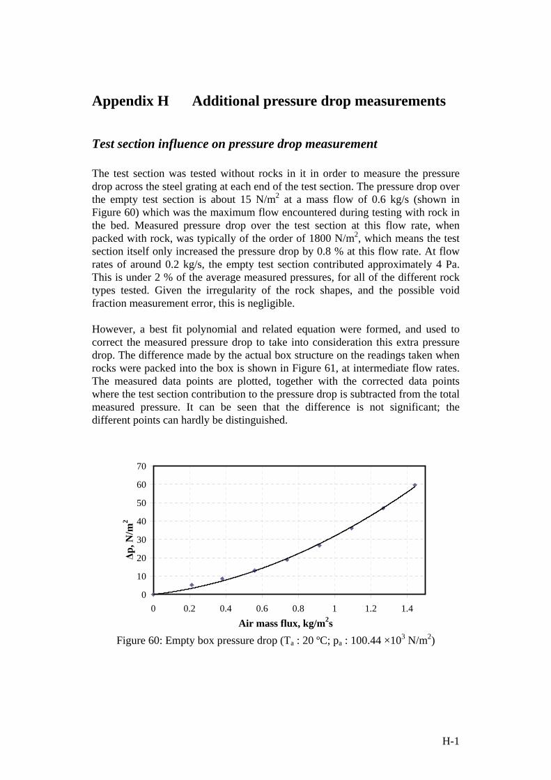
H-1

Appendix H Additional pressure drop measurements

Test section influence on pressure drop measurement The test section was tested without rocks in it in order to measure the pressure drop across the steel grating at each end of the test section. The pressure drop over the empty test section is about 15 N/m2 at a mass flow of 0.6 kg/s (shown in Figure 60) which was the maximum flow encountered during testing with rock in the bed. Measured pressure drop over the test section at this flow rate, when packed with rock, was typically of the order of 1800 N/m2, which means the test section itself only increased the pressure drop by 0.8 % at this flow rate. At flow rates of around 0.2 kg/s, the empty test section contributed approximately 4 Pa. This is under 2 % of the average measured pressures, for all of the different rock types tested. Given the irregularity of the rock shapes, and the possible void fraction measurement error, this is negligible. However, a best fit polynomial and related equation were formed, and used to correct the measured pressure drop to take into consideration this extra pressure drop. The difference made by the actual box structure on the readings taken when rocks were packed into the box is shown in Figure 61, at intermediate flow rates. The measured data points are plotted, together with the corrected data points where the test section contribution to the pressure drop is subtracted from the total measured pressure. It can be seen that the difference is not significant; the different points can hardly be distinguished.

0

10

20

30

40

50

60

70

0 0.2 0.4 0.6 0.8 1 1.2 1.4

Air mass flux, kg/m2s

∆p,

N/m

2

Figure 60: Empty box pressure drop (Ta : 20 ºC; pa : 100.44 ×103 N/m2)

H-2

0

50

100

150

200

250

300

350

0 500 1000 1500 2000 2500 3000Rep

∆p,

N/m

2

MeasuredCorrected

Figure 61: Box effect on measured pressure drop (43 mm shale, repacked; Ta : 23 ºC; pa : 100.7 ×103 N/m2)

Edge effects and repeatability of the 42 mm dolerite The effect of the wall lining on the pressure drop measurements of the dolerite is shown in Figure 62. The repeatability of the pressure drop measured before and after repacking the rocks is also shown. It can be seen that these results are of a similar trend to those for the granite and shale.

0

0.0005

0.001

0.0015

0.002

0.0025

0.003

0.0035

0.004

0.0045

0 1000 2000 3000 4000 5000 6000 7000Rep

1/K

=0.

5ρfv

s2 /∆p

Measured: original packingMeasured: repackedRUC (Du Plessis and Woudberg, 2008)Ergun (1952)Singh et al. (2006) sphericity 0.555Measured: no wall lining

Figure 62: Edge effects and repeatability for 42 mm dolerite

I-1

Appendix I Sample calculations

Wind tunnel mass flow rate The wind tunnel mass flow rate calculation is shown for pressure drops measured over nozzle 3 while the shale was tested:

Table 12: Input values for mass flow rate calculation Tf 22.2 ºC An 0.01767 m2 ∆p (test section) 573.7 N/m2 Atus 1.44 m2

pa - pn 590.1 N/m2 cpf/cvf 1.4 ∆pn 145.2 N/m2 dn 0.15 m pa (ambient pressure) 100 300 N/m2 pup 99 709.9 N/m2 µf (air viscosity) 1.81 × 10-5 kg/ms The mass flow rate through the wind tunnel is estimated from equation (5.1), where the air density at the nozzles is given by 177.1)/( == fnf RTpρ kg/m3.

The ambient air density is 184.1)/( == faf RTpρ kg/m3, which is 0.5 % larger

than the density at the nozzle. These values and those from Table 12 when substituted into equation (F.3) give Y=1.000076, and (F.2) gives gφ =0.99922.

In order to calculate a value for Cn, it is necessary to estimate a value of the nozzle Reynolds number and iterate by estimating new Reynolds numbers until the calculated number matches the estimate. If the Reynolds number is assumed to be Ren =152 000, the middle term of equation (F.1) gives a value for Cn of 0.9885. If these values are substituted into (5.1), it gives a mass flow rate of 0.32271 kg/s. The value of Ren is checked to determine if the initial guessed value is correct.

fnnfn Adm µ/Re �= =151 347, where nf Am /� =0.32271/0.01767=18.26 kg/m2s.

This is close to the guessed value of Ren. A further iteration with a nozzle Reynolds number of 151 300 gives a mass flow of 0.32269 kg/s, which is only 0.006 % different from the value estimated at Ren=152 000.

Pressure drop calculation The values of the variables given in Table 13 are used in the Ergun, RUC and Singh et al. equations shown below. The calculated pressure drop and dimensionless pressure drop for the Ergun and RUC equations may be compared with Figure 10. The inverted dimensionless pressure drop from the equation of Singh et al. is shown in Figure 12.

I-2

Table 13: Input values for pressure drop calculation

ε 0.381 G 1.5 kg/m2s Acs 0.2001 m2 µf 1.81 ×10-5 kg/ms D ( = ds) 0.0426 m L 0.5 m ρf 1.184 kg/m3 cd 1.9 ψ 0.54

The Ergun Reynolds number is 5703)1(/Re =−= εµ fer GD and the particle

Reynolds number is 3530/Re == fp GD µ . The superficial velocity

267.1184.1/5.1/ === fs Gv ρ m/s.

The Ergun equation The pressure drop is calculated from equation (3.15) as 887/ =∆ Lp N/m2/m,

where the friction factor 776.1Re/15075.1 =+= ererf . The total pressure drop

over the bed at this flow rate is then 5.4435.0887 =×=∆p N/m2. The

dimensionless pressure drop 467)5.0/( 2 =∆= sf vpK ρ , and 1/K = 0.00214.

The RUC model Equation (3.19) is used to calculate a pressure drop per meter bed length of

9353.9193.15/ =+=∆ Lp N/m2/m, or a total pressure drop over the bed of 467 N/m2. K = 491 and 1/K = 0.00203.

The correlation of Singh et al. Equation (3.20) gives a value of fs=22.74. This gives a pressure drop of

1014)/(/ 2 ==∆ DGfLp fs ρ N/m2/m or 507=∆p N/m2. The values of K and 1/K

are 534 and 0.00187 respectively.

The best fit present method for pressure drop The values given in Table 14 are used to calculate the values of c2 and c for the 42.6 mm shale, at the same mass flow rate calculated from the wind tunnel nozzle pressure drop.

I-3

Table 14: Input values best fit present method Tf 22.2 ºC (295 K) z -0.21 ∆p 573.7 N/m2 b 0.683 pa 100 300 N/m2 g 3.77×10-7

µf 1.81 × 10-5 kg/ms G 0.3227/0.2001=1.613 kg/m2s L 0.5 m R 287 J/kgK pa 100 300 N/m2 D (=ds) 0.0426 m The particle Reynolds number at this flow rate is 3796/Re == fp GD µ .

The value of c2 is calculated from the measured pressure drop by means of

equation (3.23). A value of z= -0.21 gives 731.0)/( 122 =∆= −+ bz

fzTLGpc . The

definition 1

2 2

(1 / 2 )

2

zt

z za

cRd D dc

g pε

−

+

+= , is used to calculate the value of c. The RUC

size is calculated from equation (3.16); 0500.0)1/( 3/1 =−= εsdd m. The pore

diameter is estimated from equation (3.9): 0175.0)1(/4 =−= εε vst Ad m, where

Avs=6/D. When substituted into the definition for c2, these values give c = 10.65. This is very close to the average value for c, shown in Table 6, which was calculated from all the measured pressure drop points. The value of c2 is shown graphically in Figure 14.

Heat transfer coefficient calculation Table 15: Values to calculate heat transfer parameters G 0.4669 kg/m2s Ts at t = 0 25 ºC pa 100 450 N/m2 ψ 0.54 ε 0.381 Pr 0.69 kf 0.0288 W/mK Tf (inlet) 61 ºC (334 K) D (= ds) 0.0426 m cpf 1006 J/kgK ks 2 W/mK L 0.5 m ∆x 0.0109 m ρs 2750 kg/m3 cs 820 J/kgK ∆t 1 s g 3.75 × 10 -7 kg/msKb b 0.683 These calculations are for the 42.6 mm shale, during the charging cycle, with an air mass flux of 0.4669 kg/m2s. The calculation is for the first segment of the packed bed for the first time step of charging. The Nusselt number may be calculated from correlations (4.1) to (4.6) or the Martin GLE equation (4.10). These are very similar in form, so only that of Martin GLE and Wakao et al. – equation (4.2) – is shown here.

I-4

The air density 05.1)334287/(100450/ =×== faf RTpρ kg/m3 and the air

viscosity at 61 ºC is estimated as 51099.1 −×== bff gTµ kg/ms. The particle

Reynolds number is 999/Re == fp GD µ .

The Hagen number is calculated from equation (4.14) as 20.5×106. The ratio dh/Lf, from (4.13) is 0.350. The value of xf is chosen as 0.45, the value Martin gives for spheres. When substituted into (4.10), these give a Nusselt number of 66.4, or h = 45 W/m2K. The equation of Wakao et al. - (4.2) - gives 2.63/ == fkhDNu , or h = 43

Wm2K. This is very similar to the value from the Martin GLE equation. (For a mass flux of 0.2 kg/m2s – as discussed in section 6.5 – 428/Re == fp GD µ and

the equation of Wakao et al. gives h = 26 W/m2K.) The next step is based on the heat transfer coefficient calculated from the equation of Wakao et al.: 42.7 W/m2K. In order to calculate the NTU value, it is necessary to convert h into a volumetric heat transfer coefficient: 3723== hahv W/m3K,

where 2.87/)1(6 =−= Da ε m2/m3. NTU is calculated from equation (4.8) as 3.97. If the value of NTU is adjusted to take into account the thermal resistance of the individual rocks, the Jeffreson correlation (4.27) gives NTUc = 3.63, 9 % smaller than the unmodified value, where 45.02/ == sD khDBi . If the values of ks were 3

W/mK, NTUc = 3.75, which is only 6 % smaller than the unmodified value. The adjustment of Sagara and Nakahara given in equations (4.7) and (4.9) gives a modified NTU* value of 29.3)203/(20* =+= BNTUNTU where =B 1.367 from equation (4.9). The new NTU value is 17 % smaller than the unmodified value. If ks were 3 W/mK, B = 0.911 and NTU* = 3.49, which is 12 % smaller than the unmodified value. The modification of Sagara and Nakahara is more sensitive to low particle conductivity than the correlation of Jeffreson, and it predicts a reduction in heat transfer through the packed bed that is almost double that of the prediction by Jeffreson. The fluid and solid temperatures in the inlet segment may now be calculated for the next time step. The NTUc value of 3.63 from the Jeffreson correlation is used for all NTU terms. Equation (4.24) allows the average fluid temperature in the segment to be calculated from the inlet air temperature (equivalent to Tf,i = 61 ºC in this case):

27.58)1)(2561()61( )5.0/0109.0(63.31, =−−−= −

+ eT if ºC

I-5

The value of 07588.011 )5.0/0109.0(63.3)/( =−=−= −∆− ee LxNTUη and 1489=τ s for the whole bed from equation (4.22). Equation (4.26) is solved according to the finite difference scheme presented in equation (5.9), where τ is scaled according to the segment size by the ratio Lx /∆ , which gives a time constant for each segment of about 32 s. The time step used, 1 s, is less than this, as required. The segment average temperature at the next time step, from (5.9), is

07588.01489

146

2

11

)07588.01489

146)(27358()07588.0

1489

146

2

11)(27325(

,

+

++−+=+

isT

so 077.2980012.1/)776.065.297(, =+=+

isT K or 25.077 ºC. In other words, the

rock temperature in the first segment warms by 0.077 ºC in the first time step of the charging process.

Rock heating rate in oven: heat transfer coefficient estimate The rock samples that were thermally cycled between room temperature and 500 - 520 ºC in the oven were heated by natural convection, radiation from the oven walls, and conduction from resting on the oven floor. The heat transfer by conduction is ignored, based on the assumption of very small contact area between the rock and the floor. However, the radiation from the oven walls and the natural convection heat transfer to the samples is roughly estimated to allow an effective heat transfer coefficient to be calculated and compared with that in a packed bed with forced convection. In a packed bed, the rock temperature at a given cross-section should be similar to each other; this should result in less radiation heat transfer between particles than in an oven. Mills (1999) lists some equations to calculate natural convection Nusselt numbers. For a sphere,

9/416/9

25.0

]Pr)/469.0(1[

589.02

++= Ra

Nu (I.1)

where the Rayleigh number 23 /PrPr υβ DTgGrRa g∆== . The volumetric

coefficient of expansion β = 1/Tfilm for an ideal gas, Tfilm is the film temperature and gg is the gravitational acceleration. υ is the kinematic viscosity. ∆T is the difference in temperature between the rock and the air. When the rocks are replaced in the oven they are at approximately 50 ºC. If the air properties are evaluated at the mean film temperature of (50+510)/2 = 280 ºC, Pr

I-6

= 0.69 and υ = (28.0×10-6/0.648) = 4.32 ×10-5 m2/s and kf = 0.0418 W/mK. The average rock size is about 0.05 m. The Rayleigh number is calculated based on air properties at the film temperature

3253 10377)]273280()1032.4/[(05.081.9)50510(69.0 ×=+×××−×= −Ra . When substituted into equation (I.1), this gives Nu = 13.2. The heat transfer coefficient is therefore 11/ == DkNuh f W/m2K. The heat flux per unit surface area at this

temperature difference is 546011/ =×=∆= ThAQ s� kW/m2. However, this may

over-estimate the natural convection heat transfer, as the rocks rest on the floor of the oven. If the heat transfer coefficient is estimated for a flat plate, Mills (1999) gives the relation

2.082.0 RaNu = (I.2) which is for a cooled square horizontal plate facing up. It is valid in the range 105 < Ra < 1010. If the plate dimension is assumed to be the particle size D of 0.05 m, the Nusselt number is 11 W/m2K, very similar to that predicted by equation (I.1). The initial radiation heat transfer to the rock may be estimated for the same rock and oven temperatures used above. The rock is treated as a convex grey object in a grey enclosure. It is assumed that the oven is long and the walls are all at an equal temperature of 510 ºC. The emissivity εr of the rock and oven walls is assumed to be 0.5. The heat flux absorbed by the stone is

10)(/ 44 =−= sovrs TTAQ σε kW/m2, where σ is the Boltzmann constant of 5.67

(10-8) W/m2K4. Ts is the rock temperature, 50 ºC (323 K) and Tov is the oven temperature, 510 ºC (783 K). The total initial heat flux on the rocks is the sum of that from convection and radiation: 15 kW/m2. This is the equivalent of a heat transfer coefficient of about

33/ =∆= TAQh stot� W/m2K. This is of a similar order of magnitude to the heat

transfer coefficient calculated for the shale at a mass flux of 0.4667 kg/m2s – about 42 - 45 W/m2K. It is likely that a packed bed will be used at a lower mass flux then 0.47 kg/m2s. At a mass flux of 0.2 kg/m2s, for 0.05 m particles, at an air temperature of 61 ºC,

51099.1 −×== bff gTµ , kf = 0.0288 W/mK and 501/Re == fp GD µ . The

equation of Wakao predicts a Nusselt number of 42.5, which is a heat transfer coefficient of 24.5 W/m2K. This is of a similar magnitude to the estimated heat transfer coefficient of the rock samples in the oven, so it appears that the estimated heating rates in the thermal cycling tests and the expected heating rates

I-7

in large packed beds are roughly comparable when the temperature difference between the rocks and air is large.

Steam cycle power generation If it is assumed that the average steam cycle efficiency is η = 30 % as in section 7.2 (heat energy to electrical output, with all losses taken into account), the power generated from a steam cycle may be roughly estimated from the expression

fpffe TcmP ∆= �η . fT∆ is the difference between the temperature of the air

supplied to the steam cycle from the packed bed, and the ambient temperature. The calculation is based on conditions listed in Table 9 (constant discharge mass flow rate of 224=fm� kg/s for 10 hours, and an ambient temperature of 25 ºC),

and a specific heat capacity of air cpf = 1028 J/kgK. The air supply to the steam cycle is assumed to be at a minimum average temperature of 480 ºC, which is lower than the expected average temperature, 500 ºC or more for the first 8 hours of discharging (see Figure 43 and Figure 44). The electrical power generation potential is estimated as

4.31)25480(10282243.0 =−×××=eP MWe.

If the ambient temperature were as high as 50 ºC, which may be possible under extreme conditions in arid regions, the power generation is estimated as

7.29)50480(10282243.0 =−×××=eP MWe.

Note that this ignores the fact that the air inlet temperature to the storage will be 50 ºC and not 25 ºC, which would increase the time for which the storage could provide air at temperatures above 475 - 480 ºC. Both calculations ignore the possibility of feeding the exhaust heat from the steam boiler back into the rock bed, so that the discharge air enters the rock bed at a higher temperature. This should slightly prolong the time for which the storage could provide air at above the minimum temperature. It should be noted that these calculations are idealised and do not take into account any thermal losses from storage, or other losses that may occur. Further work and analysis is required to determine the importance of these influences.