1

Performance (and) Persistence in Commodity Funds

JESSE BLOCHER*, RICKY COOPER** AND MARAT MOLYBOGA***

ABSTRACT This study documents persistent, net-of-fees, alpha-generating Commodity Trading Advisor funds focused on commodity investment (“Commodity Funds”). A new benchmark model, which includes factors established in the literature, is the baseline for performance measurement. A nonparametric bootstrap test establishes the existence of alpha that cannot be explained by luck. Performance persists 12 months out of sample, and subsequently disappears. This abnormal performance, without a reversal, indicates that persistent alpha is based in information about fundamentals, not fund flows or sentiment. These results are robust to data biases established in the literature.

Current version: August 26, 2015

*Assistant Professor of Finance, Owen Graduate School of Management, Vanderbilt University, 401 21st Avenue South, Nashville, TN 37203. **Assistant Professor of Finance, Stuart School of Business, Illinois Institute of Technology, ***Chief Risk Officer and Director of Research, Efficient Capital Management and Adjunct Faculty at the Stuart School of Business, Illinois Institute of Technology. Blocher acknowledges support from the Chicago Mercantile Exchange and the Vanderbilt’s Financial Markets Research Center. We are grateful for comments and suggestions from Craig Lewis, Nick Bollen, Bob Whaley, Luke Taylor, Adam Reed, Clemens Sialm, Vikas Agarwal, Jeff Busse, and Sohpie Shive. We benefitted from conversations with Christophe L’Ahelec. Cheng Jiang provided excellent research assistance. The authors can be contacted via email at: jesse.blocher@owen.vanderbilt.edu, rcooper3@stuart.iit.edu, and molyboga@efficientcapital.com.

2

Performance (and) Persistence in Commodity Funds

“Like most products in the liquid alternatives space, this is not a simple plug-and-play category, where any above-average fund will suffice… The challenge, as always, is finding the right manager. But it doesn't help that the managed futures space is still a very long way from enabling simple and straightforward comparisons.” - Investment News, Jan 14, 2015 “Managed futures funds shine anew, but mystery remains” "Accessing skilled managers is ever more critical – Manager selection is becoming increasingly important, as the gap between outperforming and underperforming hedge funds widens.”- Deutsche Bank, March 3, 2015 Alternative Investment Survey of hedge funds and commodity trading advisors.

Studies evaluating asset managers date back at least to Treynor (1965) and Jensen

(1968,1969), and the literature specifically assessing mutual fund managers continues to grow.

While there are some established results evaluating hedge fund managers’ skill, there exist no

studies (to our knowledge) evaluating Commodity Funds, a subset of Commodity Trading

Advisors (CTAs) that solely trade commodity futures.

There are two reasons why. First, commodity funds (and CTAs more generally) are

typically combined with hedge funds in studies of managerial skill. Assessing the skill of hedge

fund managers is difficult due to time-varying (or non-existent) market exposure, ‘catastrophe

insurance’-like returns, and no public mark-to-market for many holdings (Bollen 2013, Bollen

and Whaley 2009). Second, data for hedge funds and CTAs is typically subject to various biases,

most recently the ‘graveyard bias’ identified in Bhardwaj, Gorton, and Rouwenhorst (2014).

This paper addresses concerns in both performance measurement and data bias. To address

the measurement issue, we isolate commodity funds because they operate in an environment

much closer to mutual funds than hedge funds. Thus, they are largely free of the issues that

plague hedge fund performance assessment. Commodity funds invest in a definable set of

commodity futures contracts. This is similar to equity mutual funds that invest in a definable set

3

of publicly traded equities, but contrasts with hedge funds, which can, and do, trade any security.

Commodity futures are also publicly traded and marked to market with daily closing prices. This

is again similar to equity mutual funds, which invest in publicly traded equities, but contrasts

with hedge funds, which have great discretion on valuing their portfolios (e.g., Bollen and

Whaley 2009, Agarwal, Daniel, and Naik 2011).1

The second issue inhibiting evaluation of commodity fund managers is data bias. We

address this by obtaining monthly updates from Barclay Hedge, the largest data provider for

CTAs. Because we maintain our own graveyard database, we can control for the ‘graveyard bias’

identified in Bhardwaj, Gorton, and Rouwenhorst (2014) as well as the other biases established

in the literature. Finding persistent poor performance (discussed later) is also excellent evidence

that our sample is sufficiently de-biased.

While it is true that commodities represent a smaller market than publicly traded bonds or

equities, commodities as an asset class are becoming higher profile. Gorton and Rouwenhorst

(2006) first proposed the idea of including commodities in diversified portfolios as an equally

weighted passive index of commodities. Since then, commodity investing has grown such that

the “financialization” of commodities is now its own nascent literature (e.g., Cheng and Xiong

2014). Financial advisors are even suggesting that individuals include commodities in their

personal asset allocation.2 Yet, to our knowledge, there is still no established benchmark to

evaluate commodity fund managers or a comprehensive evaluation of their ability to deliver

alpha. This paper addresses both of these gaps.

1 Unlike mutual funds, commodity funds do take rather arbitrary levels of leverage and market exposure. This is

easily controlled for, and we discuss this difference later in the paper. 2 “Speculating on commodities can add diversity to your portfolio”, The Financial Times, June 16, 2015.

http://www.ft.com/intl/cms/s/2/eee82070-ea99-11e4-96ec-00144feab7de.html

4

To evaluate fund manager performance, we first implement and test a five-factor asset

pricing model as a benchmark for commodity manager performance measurement. The model

includes a market factor, a time series momentum factor, a spot basis factor, and high and low

term premia factors. These factors are drawn from the extant literature, based in commodity

fundamentals, and each has been shown separately to capture a risk premium embedded in

commodity futures (e.g., Szymanowska et al. 2014, Bakshi, Gao Bakshi, and Rossi 2014,

Moskowitz, Ooi, and Pedersen 2012). This factor model for commodity futures parallels Fama

and French’s now ubiquitous model for publicly traded equities (now also with five factors, see

Fama and French 2015).

We then use this five-factor model benchmark to identify commodity fund manager

performance and persistence. First, we conduct a bootstrap analysis of the distribution of alpha

t-statistics and find both top and bottom performers that cannot be explained by luck. Second, we

find that both good and bad performance persists for approximately 12 months. Annualized alpha

of the top performing quintile is 2.53%, while the same for the bottom performing quintile is -

1.94%. This performance persistence disappears after 12 months, but does not reverse. This non-

reversal indicates that commodity fund manager performance is based on information and/or

skill, rather than sentiment or other non-fundamental factor, which is often the case in mutual

funds (Blocher 2015, Lou 2012).

The closest study to ours is Bhardwaj, Gorton, and Rouwenhorst (2014). They study a

more diverse set of Commodity Trading Advisors (not just commodity funds) from 1994-2012

and find that, on average, there is no positive alpha net of fees.3 They conclude that CTAs are not

worthwhile investments and attempt to explain the (seemingly irrational) continued investor

3 This confirms earlier findings by Elton, Gruber, and Rentzler (1987,1989), which look at the average

performance of a random sample of CTAs.

5

flows into the asset class. We validate their main result that average alpha is zero, but differ in

our overall conclusion because we further investigate the whole distribution, not just the average.

This is a timely study because so-called ‘passive investment’ strategies are ascendant

(Blocher and Whaley 2015). The Wall Street Journal recently referred to passive investing as

“Goliath” and quoted a practitioner as saying that “The superiority of indexing is on the verge of

becoming something very close to a secular religion.”4 In light of such momentum around

passive investing, it is important to document how to identify valuable actively managed funds,

where they exist.

I. Background on commodity trading advisor skill and commodities’ fundamentals

Commodity Trading Advisors (also called Managed Futures, as in the opening quote) are

similar to hedge funds, with a few subtle differences. Legally, they register with the Commodity

Futures Trading Commission (CFTC) rather than the Securities and Exchange Commission

(SEC). They are only available to "Qualified Eligible Persons", similar to the SEC’s "Accredited

Investor" definition for hedge funds. CTAs are also similar to hedge funds because they have

broad discretion in terms of what securities they buy or sell short, and often use derivatives,

options, and other alternative investments. CTA managers also typically have performance

incentives in their compensation contract, though recent contracts have been less lucrative due to

increased competition. Given these commonalities, they are often included together in hedge

fund studies (e.g., Bollen and Whaley 2009).

However, commodity fund managers exhibit diverse skills similar to equity mutual fund

managers. While many employ trend-following strategies (e.g., Baltas and Kosowski 2012),

4 Investing in stocks against the indexing goliath, WSJ, April 3, 2014.

http://blogs.wsj.com/moneybeat/2015/04/03/investing-in-stocks-against-the-indexing-goliath/

6

many commodity fund managers also do fundamental research similar to their equity

counterparts.5

Fundamental equity research often involves forecasting customer demand (i.e. market

growth and market share growth) as well as the supply side of a business: personnel costs, raw

material costs, etc. Similarly, commodity fund managers investigate supply and demand for the

commodities they trade. On the supply side, they investigate factors like soil and weather

conditions for agricultural commodities and political and labor risk for extractive commodities

(metals and energy).

Consider agricultural commodities. According to an anonymous agricultural commodities

trader, there are several inefficiencies they can exploit in the market. First, early market reports

(mid-August/early-September) are often of low quality, but markets often respond strongly to

them. The skilled trader can measure this over-reaction and profit from it. Second, weather

forecasts are critical. Some traders (and hedgers) rely on a centralized weather data, but skilled

traders can gather more dispersed data from dozens or even hundreds of weather stations. Global

weather forecasts matter as well since most commodities have a global market. Third, people

generalize. An early wet season in the US typically means a poor yield, but an early wet season

in South America is less material. This type of mistake can cause over- or under-reaction by the

market that can be exploited. Finally, a skilled trader might talk to seed and fertilizer companies

about sales numbers. If sales are low of drought-resistant seeds and rain levels are lower than

average, the skilled analyst may forecast a poorer crop yield.

In some ways, commodity analysts may actually have some advantages over equity

analysts. Publicly traded equities have significant requirements for disclosure, but often the most

5 Given the pairing of trend-followers and fundamentals-based traders, the commodity futures market is likely

well described by the model of Hong and Stein (1999).

7

important information about customer demand and supplier capacity is labeled “inside

information” on which it is illegal (but profitable) to trade (e.g. Jeng, Metrick, and Zeckhauser

2003, Cohen, Frazzini, and Malloy 2008). In contrast, commodity funds are legally able to gather

important information about supply and demand, and deploy it in profitable trades. This

information is costly to gather and complicated to filter and transform into expected price

forecasts. It is also susceptible to over- and under-reaction, which gives rise to profitable

momentum and trend-following strategies.

Explaining commodity risk premia dates back at least to Keynes (1923), who proposed a

theory of Normal Backwardation. The theory of normal backwardation postulates that short

hedgers of commodities outnumber long hedgers such that natural hedgers are net short. Thus,

the natural state of the market is for futures prices to be less than expected future spot prices to

give speculators a positive expected return for assuming the price risk.6 This is also the common

‘insurance’ view of commodity futures risk premia, in which commodity futures traders are

accepting price risk from hedgers in exchange for a risk premium. Rouwenhorst and Tang (2012)

survey the extensive literature and conclude that evidence for this theory is weak.

Keynes’ theory predates modern asset pricing theory, embodied in the Capital Asset

Pricing Model (CAPM). Early studies mostly found no evidence that the CAPM applied to

commodities markets (e.g. Dusak 1973, Carter, Rausser, and Schmitz 1983), confirmed recently

by Gorton and Rouwenhorst (2006), Rouwenhorst and Tang (2012), Erb and Harvey (2006). The

explanation of commodity risk premia in the context of the CAPM remains an open question in

the commodities literature.7

6 Note that normal backwardation (futures price < expected future spot price) is different from backwardation

(futures price < current spot price). 7 There is a literature relating forwards and futures premia to the consumption CAPM model (for example, see

Cooper 1993) which reports that forward and futures contracts do respond to time varying risk premium

8

The strongest empirical evidence associates inventory with commodity risk premia in the

context of the theory of storage, which dates back to Kaldor (1939), Working (1949) and

Brennan (1958). The theory of storage links commodities futures prices to the storage decisions

of inventory holders in terms of financing and warehousing costs net a convenience yield.

Gorton, Hayashi, and Rouwenhorst (2012) provide a thorough investigation into the

fundamentals of commodity investing and find that inventory and storage are the key

fundamentals in pricing commodity risk premia, and that they show up primarily in the

commodity future’s basis. This finding features prominently in our benchmark five-factor model.

II. A factor model of commodity returns

Before we can measure the performance of commodity funds, we must first construct a

reliable benchmark. In this first section, we select factors already established in the literature and

adjust them for use in benchmarking monthly commodity fund returns. Following Szymanowska

et al. (2014), we use a spot premium factor and term premium factors to account for the futures

basis. We then add a market factor, common in the commodities literature (e.g., Bakshi, Gao

Bakshi, and Rossi 2014), and a time series momentum factor also present in several commodities

papers (e.g., Baltas and Kosowski 2012, Moskowitz, Ooi, and Pedersen 2012). Finally, we use a

monthly time series, in contrast to Szymanowska et al. who use bimonthly returns and holding

periods of up to 8 months. Overall, these adjustments result in factors that are easier to

implement with comparable explanatory power. We next discuss our data before describing these

factors in more detail.

formulations. These models, however, were never re-visited because the literature moved on to arbitrage pricing models of derivatives.

9

A. Data and computation of futures premia and returns

We utilize 21 different commodity futures obtained from Commodity Systems Inc. (CSI)

that represents all major sub-sectors of commodity markets (i.e., energy, agricultural and metals).

The contracts include Soybean Oil, Corn, Cocoa, Light Crude Oil, Cotton, Gold, Copper, NY

Harbor ULSD (Heating Oil), Coffee, Lumber, Hogs, Oats, Orange Juice, Soy Beans, Silver, Soy

Meal, Wheat (CBT only), Feeder Cattle, Live Cattle, Gasoline RBOB, and Rice Rough over the

period between September of 1987 and December of 2014. Appendix 1 provides information

about Bloomberg codes and exchanges associated with each futures market.

In constructing our factors we follow convention and consider the spot price to be the price

of the nearest to expiration contract which will expire at least two months from the current

month. This avoids problems with liquidity that can plague the pricing of shorter maturity

contracts. The two-month, four-month, and six-month contracts are then defined as the first

contract to expire at least two months, four months, and six months after the spot contract

expires.8

From the commodity price series we construct several variables, from which all the

model’s factors are constructed. We define the spot premium of the commodity as the change in

the logarithm of the spot price, si(t). Therefore, the realized spot premium of commodity i at time

t, ,ˆ ( )s i tπ , is defined as

π̂ s,i(t) = ln si(t)⎡⎣ ⎤⎦ − ln si(t −1)⎡⎣ ⎤⎦ . (1)

8 As a simple example of the above discussion, corn has contracts expiring in months 3, 5, 7, 9, 12. So in

October (10), the spot contract will be December (12), the two-month contract will be March (3), the four-month contract May (5) and the six-month contract July (7). Also, note there are some commodities with monthly expirations. In this case some expiration months would be skipped on any given date. This approach is similar to Szymanowska et al. (2014).

10

As is standard in the literature, this formulation of premium does not include any return on

the required collateral from transacting in futures contracts. Intuitively, these returns are

comparable to returns in excess of the risk-free rate, since collateral is typically reinvested at that

rate.9

The n-month basis for commodity i, ( )niy t , is defined as the logarithm of the ratio of the

n-month futures price, ( )nif t , to the spot price. Generally, the n-month maturity term premium,

,ˆ ( )ny i tπ is defined as the change in this value,

π̂ y ,i

n (t) = yin(t)− yi

n*(t −1) = ln[ fin(t) fi

n*(t −1)]− ln[si(t) / si(t −1)] (2)

This may be thought of as a calendar spread which is computed by going long the n-month

futures contract and short the spot futures contract. The futures returns themselves may be

written as

rf ,i

n (t) = ln fin−1(t)⎡⎣ ⎤⎦ − ln fi

n(t −1)⎡⎣ ⎤⎦ .10 (3)

B. Factor selection and construction

The cost of carry relationship for the futures markets allows us to break the n-month

expected futures return for commodity i into a spot premium and a term premium.11 We consider

factors for each premium in turn, starting with the spot premium. Szymanowska et al. (2014)

motivate and derive a high-minus-low factor to explain spot premia. Bakshi, Gao Bakshi, and

9 The derivation of the premium formulas in this section, as well as the formal definitions of the factors are

discussed in Appendix 2. 10 n does not always decrement to n-1 because contracts do not necessarily expire every month. 11 We show this rigorously in Appendix 2. Erb and Harvey (2006), Routledge, Seppi, and Spatt (2000), and

Fama and French (1987) establish a link between basis and commodity futures risk premia.

11

Rossi (2014) and Gorton, Hayashi, and Rouwenhorst (2012) find that market and momentum

factors are also necessary.12 Thus, to price the spot premium we choose three factors initially13:

1) A high minus low spot factor (HML), which is the average above median spot return

for the 21 commodities less the average below median spot return;

2) A market factor (MKT), which is an equal weighted average of all the commodities one

period spot return;

3) A time series momentum factor (TSMOM), which is the difference in return between

an equal weighted portfolio of commodities with positive return over the previous

twelve months and an equal weighted portfolio of those with negative return over the

previous twelve months.

Each factor is derived in detail in Appendix 2. Our HML factor is very similar to

Szymanowska et al. (2014) and Bakshi, Gao Bakshi, and Rossi (2014). In constructing the MKT

factor we follow Bakshi, Gao Bakshi, and Rossi (2014) and Gorton, Hayashi, and Rouwenhorst

(2012) by choosing an equally-weighted portfolio of all commodities as the average market

factor. Establishing a market factor for commodities is non-trivial because there is no established

weighting scheme and even popular industry indices can vary greatly in composition (Erb and

Harvey 2006). The TSMOM factor is constructed using return over the last 12 months without

12 Others who find evidence for some type of momentum factor include Erb and Harvey (2006), Asness,

Moskowitz, and Pedersen (2013), Moskowitz, Ooi, and Pedersen (2012), Fuertes, Miffre, and Rallis (2010), and Miffre and Rallis (2007).

13 There is a long and growing literature of commodities factors that price commodity returns, summarized in Rouwenhorst and Tang (2012). We do not comprehensively test all possibilities, but rather focus on the factors most commonly employed.

12

any lag because skipping one month is not relevant in futures markets.14 For robustness, we

considered variations of cross-sectional momentum, but found none that added significantly to

our model. These results are available in the online appendix.

We next consider the term premium. To price the term premium we choose two factors:

4) A high term premium factor (Hterm) consisting of the average of the 2-month, 4-month,

and 6-month realized term premia for the 10 commodities with above median returns;

5) A low term premium factor (Lterm) computed the same way as Hterm except using the 10

commodities with below median returns.

These two factors follow the intuition of Szymanowska et al. (2014) who also construct

their longer term basis factor as separate high and low factors to explain commodity term premia.

However, Szymanowska et al. compute their term structure basis factor using so-called

“spreading” returns that span the maturity difference of the computed term premia. Thus, to

explain two-, four-, and six-month term premia, they require three H factors and three L factors,

each with maturities matching those three holding periods. This has two implications. First, it is

not obvious that a set of factors that explain multi-month holding period returns will continue to

perform well explaining one month returns. Second, including six additional factors in a single

benchmark model for commodity funds is unwieldy and likely redundant. Our goal is to preserve

the economic intuition and econometric relationships while creating easily implementable

14 Jegadeesh and Titman (1993), Fama and French (1996), and Grinblatt and Moskowitz (2004) use the

common measure of the past 12-month cumulative raw return on the assets, skipping the most recent month’s return. The most recent month is typically skipped in the literature to avoid the one-month reversal in stock returns potentially driven by liquidity and microstructure issues (Jegadeesh 1990, Lo and MacKinlay 1990, Boudoukh, Richardson, and Whitelaw 1994, and Grinblatt and Moskowitz 2004). However, excluding the most recent month of returns is irrelevant for commodities (Asness, Moskowitz, and Pedersen 2013) and, thus, we define momentum measure either as the cumulative raw return over the last 12 months without skipping the last month.

13

factors. Our results will demonstrate that our factors, though simpler, maintain power in

explaining futures returns.

Intuitively, our three (total) basis factors represent the spot basis (the HML factor) and the

equally-weighted average of the expected change in spot basis (Hterm and Lterm) across different

time horizons. Thus, while computed monthly, theoretically they should still capture both the

spot and term premia of commodity returns.

We summarize our factors in Table I. For all asset pricing tests, we apply Newey and West

(1987) corrections for heteroskedasticity and autocorrelation with 12 lags because there is a

pronounced seasonal effect in commodities (Gorton, Hayashi, and Rouwenhorst 2012). The

monthly excess return for almost every factor is modestly positive, but statistically different from

zero. Only the market factor is negative, but insignificant. The factors are also only modestly

correlated with each other, with the highest correlation in the entire matrix equal to 0.40.

C. Results of factor asset pricing tests

While the literature provides compelling evidence for our factor model, it has not been

tested in the form we propose. A factor model that prices commodity returns should have an

intercept of zero on average - i.e. there should be zero alpha, both economically and statistically.

We start with our test assets: portfolios sorted on basis and momentum. Since the literature

has converged on basis and momentum as the two key characteristics explaining commodity

returns, we focus on those two for brevity.15 Summary statistics are in Table II. Both sets of

portfolios are monotonically ordered with statistically significant high-minus-low portfolio

returns of 0.84%, with t-statistics of 2.7 (Basis) and 2.56 (Momentum).

15 Szymanowska et al. (2014) rigorously test a variety of other test assets based on other fundamentals such as inflation, liquidity, and open interest, etc.

14

Table III presents the results of running regressions using various combinations of our

factors explaining spot premia of basis-sorted portfolios. The dependent variable in these

regressions is the spot premium. Panels A-C use single factors: HML, MKT, and TSMOM,

respectively. HML prices the portfolios well with small and insignificant alpha for all 4

portfolios. MKT has higher R2 but also larger alphas. The TSMOM factor cannot price the B1

and B2 portfolios and has R2 mostly close to zero.

Combining factors increases the explanatory power. In Panel D, the HML and MKT do an

excellent job pricing the test assets. Alphas are very low (magnitude of 0.01-0.05% monthly) and

highly insignificant (t-statistics of magnitude 0.38 or less) with large R2 (0.71-0.75). Panels E

and F pair the MKT and TSMOM factors and the HML and TSMOM factors, respectively.

Neither pair performs particularly well in one or more dimensions (magnitude of alpha, statistical

significance, and R2). Panel G combines all three factors, with the result that the alpha is driven

to nearly zero with very small t-statistics, though there is little change in R2. Regardless of this

result, we include TSMOM because it is justified more substantively in later tests.

Table IV repeats the analysis but with Momentum sorted portfolios. The interpretation is

largely the same, though the results are not quite as strong. TSMOM is the strongest solo

performer, as both HML and MKT have some trouble pricing the M1 portfolio (t-statistics

of -1.93 and -3.96). The combination of TSMOM and MKT (Panel E) results in insignificant

t-statistics, and the combination of all three factors gives alphas close to zero, though higher than

in Table II. From a t-statistic perspective alone, one could argue that TSMOM and MKT by

themselves price momentum portfolios best. However, HML is important for basis sorted

portfolios and lowers the overall alpha of momentum-sorted portfolios.

15

In unreported results, when we repeat the analysis using term premia instead of spot

premia, the HML factor no longer prices portfolios sorted on basis. However, Table V confirms

that when we use Hterm and Lterm, all portfolios are priced with alpha near zero and nearly all

alphas have insignificant t-statistics, confirming Szymanowska et al. (2014). Table V also

confirms that combining the two term premium factors into a single HMLterm does not price the

test assets and thus is rejected.

The contrast between the left column of results (the HMLterm factor) and right column of

results (Hterm and Lterm separate) is striking. In the right column, 9 of 12 computed alphas are

0.04 or less in absolute value. Only two are statistically significant and both are small in

economic significance (0.08% and -0.1% monthly). In contrast, the HMLterm factor in the left

column fails to price all but two of the test portfolios. While the performance of our Hterm and

Lterm factors is not quite as good as those of Szymanowska et al. (2014), we believe the trade-off

for investability and parsimony is worth the small reduction in pricing ability.

As a final test of our factor model, we regress the factors on each other. If a subset of

factors can completely “price” the remaining factor (i.e. set the intercept statistically equal to

zero) then the factor is redundant in the model. Table VI shows the results. Panels A and B test

the HML, TSMOM, and MOM factors. MOM is a typical cross-sectional momentum factor

defined as the top quartile portfolio less the bottom quartile portfolio of commodities sorted on

the previous twelve months of spot returns. Panel A, row 1 clearly shows this MOM factor as

redundant and fully priced by the MKT, HML, and TSMOM factors. The same cannot be said,

however, of TSMOM and HML, both of which show a statistically significant intercept in rows 2

and 3 of Panel A.

16

Further bolstering the case for our chosen factors, Panel B again shows TSMOM as

necessary when we include the other four factors as independent variables. The t-statistic is 3.06.

HML seems redundant with a low t-statistic, but given our previous evidence pricing test assets,

we nevertheless keep HML in the specification. Finally, in Panel C, we test Hterm and Lterm. In all

cases, the intercept is statistically significant, with t-statistics above 3 in all four rows. Overall,

we see this as additional evidence for our chosen five-factor model including MKT, HML,

TSMOM, Hterm, and Lterm.

III. Performance (and) Persistence in Commodity Funds

Having established our benchmark, we next turn to measuring the performance and

performance persistence of commodity funds. First, we summarize our dataset that accounts for

the known biases in the literature, including ‘graveyard’ bias. Then, we describe our

bootstrapping methodology and results to establish the existence of skill as distinct from luck.

Finally, we discuss our performance persistence results. The first result derives from an OLS

specification and for robustness, we re-run the specification in a Bayesian analysis. In addition to

the overall sample results, we also test metal and non-metal commodity subsamples.

A. Data

In this study, we use the Barclay Hedge database, the largest publicly available database of

Commodity Trading Advisors (CTAs). This is indicated by their usage as the benchmark for

total Assets Under Management (AUM) held by CTAs (e.g., Bhardwaj, Gorton, and

Rouwenhorst 2014, Hurst, Ooi, and Pedersen 2013).16 Our de-biased, final sample of

Commodity Funds includes 183 unique active and defunct funds over the period between

16 Joenväärä, Kosowski, and Tolonen (2014) evaluate five commonly used databases of hedge funds including

Barlcay Hedge, TASS, HFR, Eurohedge and Morningstar. They find that the Barclay Hedge is the highest quality database in many respects including least likely to suffer from survivorship bias.

17

December of 2006 and December of 2014 and represents 24% of the Barclay Hedge database by

AUM. Because we require 24 months of data for evaluation, our first performance prediction is

for January 2009.17

To get to this final sample, we first filter on fund category. We eliminate multi-advisors

(Funds of Funds) and select funds that specialize in commodity trading by picking funds with

classifications of Technical – Energy, Fundamental – Energy, Technical – Agricultural,

Fundamental – Agricultural, Technical – Financial/Metals, Fundamental – Financial/Metals

available in the Barclay Hedge database. See Appendix 1 Table II for a full listing of categories

both included and excluded.

We further limit the study to the funds that report returns net of all fees to ensure

comparability of returns. As a final filter, we exclude the bottom 20% of funds based on AUM.

This filter serves two purposes: first, it controls for incubation bias and other small-fund effects

and second, it makes our study most relevant for institutional money managers who typically

will not invest in the smallest funds. This dynamic AUM threshold approach is more appropriate

than a fixed AUM approach commonly used in the literature (Kosowski, Naik, and Teo 2007)

because the level of AUM has fluctuated over the last 10 years.18

We minimize selection bias by using the largest, highest quality data available on the

market. To control for survivorship bias, we include the graveyard database that contains defunct

funds. Additionally, to eliminate the ‘graveyard bias’ identified by Bhardwaj, Gorton, and

Rouwenhorst (2014) we obtain monthly updates to the Barclay Hedge database starting in

17 As a reference point, Bhardwaj, Gorton, and Rouwenhorst (2014) have a final sample from Barclay Hedge

that represents 21% of the total by AUM. If there is concern about small sample size, all of our results are the same in the full sample starting from 1993, available in the online appendix. This sample is subject to graveyard bias prior to 2006, however.

18 We obtain similar results with thresholds of 15%, 25% and 30%, available upon request. Kosowski, Naik, and Teo (2007) also use a dynamic median calculation to separate large and small funds. A table listing the exact AUM threshold and number of fund included/excluded due to this screen is available in Appendix 1.

18

November 2006 through December 2014. Thus, our set of closed funds only grows even if funds

request their history deleted from the graveyard dataset.19

Backfill bias also arises due to the voluntary nature of self-reporting. Typically, funds go

through an incubation period during which they build a track record using proprietary capital.

Fund managers choose to start reporting to a CTA database to raise capital from outside

investors only if the track record is attractive and they are allowed to “backfill” the returns

generated prior to their inclusion in the database. Since funds with poor performance are unlikely

to report returns to the database, this behavior results in the incubation/backfill bias.

We combine two standard approaches to mitigate backfill and incubation biases. First, we

apply a technique suggested by Kosowski, Naik, and Teo (2007) that eliminates the first 24

months regardless of the level of AUM20. Second, we include funds that reach US$ 1 million

AUM normalized to 2014 values as in Fama and French (2010). Once a fund passes the AUM

minimum (even if that occurs in the first 24 months), it is included in all subsequent tests to

avoid creating selection bias.

Finally, we account for reporting delays as in Molyboga, Baek, and Bilson (2014). If we

build a portfolio in December of 2009, we use data through the end of November 2009 since that

is the most recent data available to practitioners at the time of portfolio formation. Forming

“December” portfolios with December data is common in the literature but not implementable.

19 Bhardwaj, Gorton, and Rouwenhorst (2014) document a new ‘graveyard bias’ which arises when CTAs

request that their entire history be deleted, including that in the graveyard database. Since these data providers are beholden to these CTAs to voluntarily report, such requests are granted.

20 Bhardwaj, Gorton, and Rouwenhorst (2014) note that using the initial reporting date is a better control for backfill bias, but this is only available in the smaller TASS database, not more comprehensive Barclay Hedge dataset we use. Brown, Goetzmann, and Park (1998) find 27 month incubation periods for CTAs, so we view a 24 month cutoff as a close approximation to the initial reporting date. We view this as an acceptable and necessary trade-off to use the larger dataset.

19

Table VI provides summary statistics for our sample of commodity fund managers. We

have 183 unique funds divided into three categories: Energy, Agricultural, and Metals. The

sample is slanted towards Metals, but we show later that our results are robust to this. While all

have positive excess returns, none are statistically different from zero on average, which is

consistent with the literature. Skewness is slightly positive on average and excess kurtosis differs

from the normal distribution on more than half the population of funds, confirmed by the Jarque-

Bera test statistic. 21

For robustness, we conduct a Bayesian, seemingly unrelated assets (SURA) analysis. For

the seemingly unrelated assets, we use monthly returns of the Barclay Agricultural Traders index

and the Barclay Financial and Metals Index during the period between December of 1993 and

December of 2014 reported in the Barclay Hedge database. The Barclay Agricultural Traders

Index is an equal weighted composite of funds that trade agricultural markets such as grains,

meats and foods. In 2014 the index included 40 agricultural funds. The Barclay Financial and

Metals Index is an equal weighted composite of funds that trade primarily financials and

metals.22 In 2014 the index included 76 funds. Figure 1 Panel A displays the time trend of these

commodity index returns versus the S&P 500, with all three normalized at 100 in December of

1993, which is the beginning of the sample of index returns. Panel B starts in October 2006, just

before our CTA sample begins, again with each index re-normalized to 100. For the risk free rate

we use the 3-month Treasury bill (secondary market rate) series with ID TB3MS from the Board

of Governors of the Federal Reserve System.

21 Excess kurtosis is computed as Kurtosis minus 3, which is the kurtosis of the Normal distribution. 22 The industry terminology for these is ‘managed programs.’ They are not organized like ‘funds’ in the mutual

fund sense, but they are conceptually similar and the difference is irrelevant here.

20

B. Commodity fund outperformance with bootstrapping

To assess the performance of commodity funds, we first turn to a bootstrap analysis.

Bootstrap tests compare the distribution of the actual alphas and t-statistics of alpha to the

distribution of the alpha and t-statistics of alpha generated using bootstrap simulations of returns.

The bootstrap distribution is designed to have the same properties as the original distribution but

with true alpha set to zero for each fund. Alpha is always calculated with reference to our five-

factor benchmark model, and is set to zero by subtracting each fund’s estimate of alpha from its

returns. This bootstrap distribution then generates the return distribution funds exhibit assuming

the expected value of alpha were actually zero. This provides a baseline for comparison.

A bootstrap approach has several benefits. Bootstrap analyses have the advantage of not

requiring ex-ante assumptions about the distribution of returns. The commodity funds we study

are typically included in hedge fund studies, which have been shown to have non-normal

distributions of various performance metrics (e.g., Kosowski, Naik, and Teo 2007). We confirm

this in Table VII, which shows that over half of our sample is non-normal using the Jarque-Bera

test of skewness and kurtosis. A bootstrap approach also allows a robust approach to dealing

with possibly unknown serial correlation and heteroskedasticity in the residuals from a

performance regression. Table VI shows that 14.2% of our sample exhibits heteroskedasticity as

measured by the Breusch-Pagan test and 19.7% exhibits autocorrelation according to a Ljung-

Box test. Finally, the bootstrap approach has already proven useful in both mutual funds and

hedge funds (e.g., Kosowski et al. 2006, Kosowski, Naik, and Teo 2007, Fama and French

2010).

Our bootstrap sampling approach combines the methods outlined in Fama and French

(2010) and Kosowski, Naik, and Teo (2007) (which is based on Kosowski et al. 2006). Each of

these three studies uses slightly different methodologies to generate the bootstrap distribution

21

based on how they choose to handle cross-correlation and auto-correlation inherent in most

security returns.

With mutual fund data, Kosowski et al. (2006) perform independent simulations for each

fund which guarantees that the number of months in simulated returns for each fund exactly

matches the fund’s actual length of track record but implicitly assumes zero correlation of alpha

estimates across funds in the same month. Fama and French (2010) critique this approach, and

instead draw a single month’s cross-section of adjusted returns, which has an important benefit

of capturing the cross-correlations of fund returns. This approach preserves the impact of cross-

correlation on the estimated distribution of the fund alpha t-statistic. However, Fama and French

capture none of the serial correlation in the data which is insignificant for their mutual fund

context but is important for commodity funds. The Fama and French approach also likely creates

problems in a dataset with short histories and high attrition, which is a characteristic of CTAs

and hedge funds but not mutual funds.

Kosowski, Naik, and Teo (2007) extend Kosowski et al. (2006) to account for both cross-

sectional and serial correlations by sampling cross-sectional blocks of data instead of single

months. We combine both approaches and follow Fama and French (2010) by drawing a single

month’s cross-section of adjusted data and Kosowski, Naik, and Teo (2007) by drawing blocks

of three and six months to preserve some of the necessary autocorrelation. Thus, we define a

simulation run as a random sample with replacement of 97 months drawn from 97 calendar

months from December 2006 through December of 2014 of the adjusted dataset with true alpha

of zero. We eliminate all funds that have less than 12 months of returns in our simulated dataset.

We evaluate funds based on both alpha and the t-statistic of alpha. Alpha is the typical

measure of economic significance when evaluating fund performance (hedge fund, mutual fund,

22

commodity fund). But high alphas can arise in funds with shorter histories and thus have lower

t-statistics indicating statistical insignificance. The t-statistic of alpha, however, corrects this

problem by normalizing estimated alpha by the estimated precision of alpha. The t-statistic is

also related to the information ratio of Treynor and Black (1973), which is commonly used by

practitioners to rate fund managers (Grinold and Kahn 2000, Goodwin 1998).

C. Performance results via bootstrapping

We present our results graphically first in Figure 2. This figure plots the bootstrapped

distribution of t-statistics, centered at zero, along with the actual distribution of t-statistics. In

Panel A, we plot the distribution for the full sample from December 1993 to December 2014.

This plot illustrates the effect of our de-biasing of the data. Panel A clearly has a nonzero mean

and much fatter tails, particularly in the positive direction. Panel B is December of 2006 to

December 2014, which is our de-biased (and primary) sample, and shows how de-biasing the

data moves the mean much closer to zero. Panel B also shows that after removing bias from the

data, there is ‘fatness’ in both the lower and upper tail, which we next investigate more

rigorously.

The statistics that reinforce the conclusions observed in Figure 2 Panel B are displayed in

Table VIII. The first row presents the rank ordered t-statistics from the actual fund regressions.

The second row reports the p-values based on the bootstrapped distribution of t-statistics.

Consider the upper tail first. The t-stat in the first percentile is significant at 0.18% level, and the

third percentile is significant at the 1.30% level. The 5th percentile of t-statistics is significant at

the 3.14% level. These all exceed what we would expect from mere chance. At the lower end of

the distribution, we see a similar pattern of under-performance. The bottom first percentile is

significant at the 1.48% level and the third percentile is significant at the 2.10% level. This poor

23

performance validates the effect of our de-biasing work and also motivates the careful selection

of commodity fund managers.

Next, we report the ranked alpha estimates, with p-values based on the bootstrapped

distribution. The results are similar, and equally strong. The top 1% alpha of 3.29% per month is

significant at the 0.10% level and the third percentile alpha of 1.69% is significant at the 1.02%

level. The bottom 1% alpha of -2.67% is significant at the 0.2% level and the bottom 5% alpha

of -1.49% is significant at the 1.24% level. Overall, we view this as positive evidence of

performance (good and bad) that cannot be explained by simple statistical variation (i.e. luck).

D. Performance persistence

Having established the existence of outperformance through nonparametric tests, we turn

to establishing performance persistence, both positive and negative. To establish persistence, we

perform a quintile analysis using OLS regression as in Carhart (1997), with Newey and West

(1987) corrected standard errors. For robustness, we also estimate alphas using the Bayesian

SURA methodology of Pastor and Stambaugh (2002) as implemented in Kosowski, Naik, and

Teo (2007). The detailed Bayesian methodology is described in Appendix 3.

We start with graphical results, available in Figure 3, panels A and B. In Panel A, we sort

based on alpha computed over the previous 24 months and then plot cumulative unleveraged

returns over the subsequent twelve months (skipping one intervening month due to reporting

delays). 23 Performance is split into five quintiles, and all portfolios are normalized to start at 0.

The figure shows the top performing quintile exhibiting phenomenal cumulative returns while

the middle 3 quintiles cumulative returns are approximately 0. The lowest performing quintile

23 “Unleveraged Returns” - Commodity funds use margin to trade futures, forwards and options without incurring the cost of borrowing. Because of the cash efficiency of margin, fund managers often let institutional investors customize the level of exposure desired. Performance of all funds is normalized to 15% annualized volatility level (see Appendix 4 or Molyboga, Baek, and Bilson (2014) for details).

24

ends up significantly trailing the others. While alpha remains a key performance metric, the

t-statistic of alpha is the more rigorous measure, presented in Panel B. This figure shows clear

differentiation of the top performing portfolio vs. the other four, all of which cumulate negative

returns over the out-of-sample period.

Table IX (OLS estimates) and Table X (Bayesian estimates) tabulate the statistical analysis

of performance persistence observed in Figure 3. In each table, we present the annualized alpha

estimates with portfolios sorted on the t-statistic of alpha over two time periods. In Panel A, we

estimate annualized alpha for months 1-12 after quintile portfolio formation. In Panel B, we

estimate annualized alpha for months 13-24 post-formation. Table IX Panel A shows a positive

alpha of 2.53% for the top performing quintile (portfolio I) with a t-statistic of 3.31 and Sharpe

Ratio of 1.12.24 At the bottom end, the lowest performing quintile (portfolio V) yields an

annualized alpha of -1.94 and a t-statistic of -1.65, which is significant at the 5% level (one-sided

test). The Sharpe Ratio is -.26. The hedge portfolio (I-V) shows even stronger results, but is for

informational purposes only since it is not possible to short these funds. Finally, we see that

overall alpha for the whole sample, regardless of performance, is 0.28% with a t-statistic of 0.36,

not significantly different from zero. This corroborates the findings of Bhardwaj, Gorton, and

Rouwenhorst (2014) who find no outperformance, on average, among CTAs.

Panel B displays results for the subsequent 12 months (13-24). The purpose of this

analysis is to further understand the source of commodity fund manager performance. If it is

based in fundamental drivers of value, then we would expect performance to either continue or to

diminish to zero as investors allocate money to top-performing funds thus eroding their ability to

continue to deliver alpha, as in Berk and Green (2004). Alternatively, if abnormal performance is

24 This may seem unconditionally high, but other work in commodities has shown that this estimate is well

within a reasonable range for this market (e.g., Neuhierl and Thompson 2014).

25

non-fundamental, and instead based on fund-flows driving up prices or other sentiment-based

explanations, we would expect performance to revert as in Blocher (2015). Empirically, we find

evidence that abnormal returns are based in fundamentals, with all five quintiles exhibiting 13-24

month alpha indistinguishable from zero. The highest t-statistics is 1.38 (portfolio III) and none

of the others are above 1. This result shows that the skill displayed by these fund managers is

based in fundamentals.

The Bayesian estimates, which we expect to be more immune to model misspecification,

are presented in Table X. In Panel A, The top quintile alpha is 2.31% with a t-statistic of 1.72.

The bottom quintile (portfolio V) has an alpha of -1.67% and a t-statistic of -1.91. Each is

significant at the 5% level in a one-sided test. We again see the same result for months 13-24

post-formation. All t-statistics are less than 1, though the alpha estimates are still ordered from

portfolio I to V. This indicates that there may be some additional persistence early in the period,

but it is minimal. It also confirms the earlier result that skill is based in fundamental analysis

since the returns to top-performing funds do not subsequently mean-revert. If anything,

according to the Bayesian analysis, there is further upward drift among top performers.

In Tables XI and XII, we show the same results, but for subsamples of Non-Metals and

Metals. As can be seen in Table VII, our sample is skewed toward CTAs trading metals

commodities. Tables XI and XII show that our result applies broadly to both metals and non-

metals. In Table XI (non-metals), the results are even stronger than the full sample. The top

performing quintile in Panel A (OLS Estimates) has an annualized alpha of 4.08% and a

t-statistic of 3.49. The bottom quintile has an alpha of -3.48% with a t-statistic of -1.65,

significant in a one-sided test. The Bayesian estimates in Panel B of Table XI give similar results

with top and bottom alphas of 2.76% and –4.26%, respectively, and t-statistics of 1.89 and -2.30,

26

respectively. In Table XII, focusing on Metals CTAs gives similar results. The top and bottom

OLS-estimated alphas are 2.80% and -1.89% respectively, with t-statistics of 2.78 and -1.11,

respectively. Panel B shows Bayesian estimates, with top and bottom alphas of 2.72%

and -1.96%, respectively, and t-statistics of 1.63 and -1.91, respectively. Full-sample alphas are

indistinguishable from zero across all estimation methods and subsets, confirming that

commodity funds do not outperform on average, regardless of grouping.

Finally, to demonstrate again the robustness of the de-biasing of the data, we compare the

quintile sorts of t-statistics in our shorter, de-biased sample versus the full sample. There are two

differences in these datasets. First, obviously, the time frame is different, but second, the full

sample is subject to graveyard bias prior to 2006. All else is held constant.

The results are interesting in that the significant differences between the two are in the

middle three quintiles. The difference between the upper and lower quintiles is noticeable, but

not significant. It is also interesting to see that in the full (biased) sample, Quintiles I-III are all

positive and significant, whereas in the unbiased sample they are not. However, Quintile V has a

far greater magnitude of significance in the unbiased sample, and the difference from Quintile 1-

V remains significant in both samples.

This analysis is far from comprehensive, but it is suggestive. It could be that including the

older time period itself is what introduces the upward bias. But at least our de-biasing efforts

introduce a correction in the right direction when data are manually adjusted for survivorship

bias.

27

IV. Conclusion

We have shown both performance and performance persistence in commodity funds.

Investors who want to differentiate the best and worst commodity funds ex ante can reliably do

so. Given literature has shown that CTAs do not outperform on average, this is an important

result for commodity investors. Top performing funds predictably generate approximately of

2.5% in annualized alpha with a Sharpe Ratio of 1.12.

These results cannot be attributed to luck. We show that the distribution of actual fund

returns is different from a simulated bootstrapped distribution with alpha set to zero. This

difference shows up both in the upper and lower tails, with both top (bottom) funds generating

much better (worse) performance than would be expected by simple statistical variation in the

distribution. A Bayesian analysis incorporating seemingly unrelated assets refines our estimates

of alpha, giving additional robustness against model misspecification. Our results hold when run

on subsets of our data for both Metals and non-Metals.

We also contribute a monthly, implemental, five-factor model of commodity returns. Our

factors include a market factor, a spot HML factor, time series momentum, and Hterm and Lterm

factors based on returns to calendar spreads to price the term premia inherent in commodity

futures.

We believe our results are intuitive. Gorton, Hayashi, and Rouwenhorst (2012) (among

others) have shown that the risk premia of commodities, and basis in particular, is strongly

linked to inventory and storage costs of the underlying commodities. It is possible for motivated

commodity traders or investors to gather information on expected inventories and storage of

commodities. Thus, it stands to reason that informed investors can profitably trade on that

information.

28

We make no claims about managerial skill as in Berk and van Binsbergen (2015), which

we leave to future research. Our focus is not on identifying managerial skill per se, but rather the

fund selection problem of the fund investor who wants to maximize risk-adjusted return to her

portfolio. Specifically we have in mind an institutional investor, typically a large pension fund or

asset manager, who needs to choose a Commodity Fund for the portion of assets it wants to

allocate solely to commodities. Given that the recent performance of passive investments in

commodities has been poor25, our conclusion that active management in commodities can be

profitable is indeed timely.

25 “Investment: Revaluing Commodities”, The Financial Times, June 3, 2015.

http://www.ft.com/intl/cms/s/0/a6ff2818-094c-11e5-8534-00144feabdc0.html

29

Appendix 1: Supplemental tables

Table A1.I List of Commodities included in study.

Column 1 is the name, column 2 is the exchange on which they are traded, column 3 is the Bloomberg symbol, column 4 is the Commodity Systems, Inc (CSI) symbol.

Name Exchange BB symbol CSI Data Symbol

Corn CBOT C C2Rice Rough CBOT RR RR2Lumber CME LB LBWheat CBOT W W2Oats CBOT O O2Coffee ICE-US KC KC2Cocoa ICE-US CC CC2Cotton ICE-US CT CT2Hogs Lean CME LH LHSoybean Oil CBOT BO BO2Orange Juice ICE-US OJ OJ2Silver COMEX SI SI2Gold COMEX GC GC2Soybeans CBOT S S2Feeder Cattle CME FC FCCattle Live CME LC LCNY Harbor ULSD NYMEX HO HO2Crude Oil Light NYMEX CL CL2Soybean meal CBOT SM SM2Copper HG COMEX HG HG2Gasoline RBOB NYMEX XB RB2

30

Table A1.II List of Commodity Trading Advisor Categories

Listed are the categories for CTAs available in Barclay Hedge, along with counts of unique funds included in each category. The first group lists the categories included in our study, the second group those excluded.

Categories

Unique Funds in Dataset

Included in Study 571 Fundamental - Agricultural 73 Fundamental - Energy 36 Fundamental - Financial/Metals 112 Technical - Agricultural 14 Technical - Energy 13 Technical - Financial/Metals 323 Excluded from Study 2,390 No Category 228 Arbitrage 50 Discretionary 53 Fundamental - Currency 121 Fundamental - Diversified 144 Fundamental - Interest Rates 12 Option Strategies 153 Stock Index 178 Stock Index,Arbitrage 2 Stock Index,Option Strategies 4 Systematic 76 Technical - Currency 300 Technical - Diversified 1,050 Technical - Diversified,Currency 1 Technical - Diversified,Financial/Metals 1 Technical - Interest Rates 17 Grand Total 2,961

31

Table A1.III Impact of annual threshold - counts of funds included and excluded by year

This table presents the threshold level of assets under management at the bottom quintile. It also lists the number of funds with at least 24 months of returns included in the dataset and the corresponding number omitted due to this cutoff. While 20% is an arbitrary cutoff, results with the cutoff set at 15%, 25%, and 30% are available upon request and confirm our results.

Year

AUM threshold

($M)

Number of funds

Included

Number of Fund

Excluded1996 2.03$ 75 191997 2.31$ 71 181998 1.87$ 65 161999 2.99$ 64 162000 2.69$ 66 172001 2.31$ 62 162002 2.03$ 62 162003 2.79$ 62 162004 3.91$ 72 182005 2.85$ 86 222006 2.55$ 86 222007 2.64$ 93 232008 3.74$ 91 232009 6.61$ 99 252010 4.00$ 104 262011 4.64$ 96 242012 2.70$ 112 282013 3.00$ 113 282014 3.88$ 104 26

32

Appendix 2. The Cost of Carry Model, Risk Premia, and Factor Definitions

The cost of carry model may be defined as

A2.1) fin(t) = si(t)e

yi (τ )dτt

t+n

∫

Where y(t), the time t instantaneous cost of carry is composed of the risk free rate, the storage

rate for the commodity i, and a generally negative rate known as the convenience yield. The spot

price si(t) is the true underlying commodity price and !!fin(t) is the futures price with maturity n.

The total cost of carry over the life of the contract is summarized by the basis, defined as

A2.2)

yin = ln fi

n(t)⎡⎣ ⎤⎦ − ln si(t)⎡⎣ ⎤⎦ = yi (τ )dτt

t+n

∫

Taking derivatives and rearranging yields the equation

A2.3) [ ]ln ( ) ln ( )n ni i id f t d s t y⎡ ⎤ = +⎣ ⎦

If we now consider small discrete time changes (so A2.3 is still approximately correct), we can

write the expected spot premium as

A2.4) 1, ( ) ln( ( 1) ln( ( ) ( )s i t i i it E s t s t y tπ ⎡ ⎤= + − −⎣ ⎦ ,

and the expected term premium as

A2.5) 1 1, ( ) [ ( ) ]n n ny i t i i it E y t y yπ −= + − .

A2.4 gives the premium as the difference between the expected change in the spot price and the

one period basis. A2.5 gives the premium as the deviation from the expectation hypothesis.

We can now expand A2.3 to expected futures return as

A2.6) 1 1 1 1,[ ( 1)] [ ( 1) ( )] [ ( 1) ( 1) ( ) ( ) ( ) ( )]n n n n n

t f i t i i i i i i i iE r t E f t f t E s t y t s t y t y t y t− −+ = + − = + + + − − + −

This reduces into

33

A2.7) , , ,[ ( 1)] ( 1) ( 1)n nt f i s i y iE r t t tπ π+ = + + + ,

which is in terms of risk premia. Recall that we have defined the spot commodity to be the

nearest term futures contract, and this definition includes the true spot price plus the one period

cost of carry. Thus, our spot premium and term premia measures correspond to realizations of

the premia in equation A2.7.

The three factors considered in this paper to price the spot premium are:

A2.8) , ,1 ˆ ˆ( ) ( ) ( )s i s i

i H i Lg

HML t t tN

π π∈ ∈

⎡ ⎤= −⎢ ⎥⎣ ⎦∑ ∑

where H is the set of commodities that have spot return above median, L is the set of

commodities that have spot return below median, and Ng is the number of commodities in each

group. Since we have 21 total commodities, Ng is 10. Our market factor is simply

A2.9) ,1

1 ˆ( ) ( )N

s ii

MKT t tN

π=

= ∑

where N, the number of total commodities, is 21. We define momentum as

A2.10) , ,1 1ˆ ˆ( ) ( ) ( )s i s i

i P i Lpos neg

TSMOM t t tN N

π π∈ ∈

⎡ ⎤⎡ ⎤ ⎡ ⎤= −⎢ ⎥⎣ ⎦ ⎣ ⎦⎢ ⎥⎣ ⎦

∑ ∑

where neg and pos refer to the set of commodities with positive and negative trailing 12 month

returns. Npos and Nneg refer to the number of commodities in each group.

The two factors used in this paper to price the term premium are

A2.11)

,2,4,6

,2,4,6

1 1 ˆ( ) ( )3

1 1 ˆ( ) ( )3

nterm y i

i H ng

nterm y i

i L ng

H t tN

L t tN

π

π

∈ =

∈ =

⎡ ⎤= ⎢ ⎥

⎣ ⎦⎡ ⎤

= ⎢ ⎥⎣ ⎦

∑ ∑

∑ ∑

34

where H is the set of commodities with above median returns, and L is the set of commodities

with below median returns. Ng is the number of commodities in each group, which again is 10.

Appendix 3: Bayesian Methodology

The precision of performance measures such as the t-statistic of alpha or Sharpe ratio

suffers from short track records of commodity traders. Pastor and Stambaugh (2002) introduce a

powerful Bayesian framework that improves accuracy of estimates by incorporating return

information of seemingly unrelated assets that are not explicitly used in the definition of funds’

alphas but have longer time histories. The precision gains from the framework are the highest

when the seemingly unrelated assets, or non-benchmark passive assets, have high correlation to

fund returns and, therefore, industry indices are good candidates for that role as suggested in

Pastor and Stambaugh (2002) for mutual funds and Kosowski, Naik, and Teo (2007) for hedge

funds. In this paper we use Barclay Agricultural Traders index and the Barclay Financial and

Metals Index as seemingly unrelated assets, or non-benchmark passive assets.

Following Pastor and Stambaugh (2002), we denote , the vector of returns in

month on seemingly unrelated assets and , the vector of returns in month on

benchmarks (or factors). Non-benchmark assets are regressed on the benchmarks, using the

whole time series available at the time of analysis26:

,

with the variance-covariance matrix of the residuals denoted by . In our paper we utilize

our four-factor model as the benchmark specify the two industry indices as non-benchmark

26 If analysis began at the end of December of 2012, the complete dataset available at the time of analysis would’ve been the period between December of 1993 and November of 2012 (108 months). In contrast individual funds are evaluated using only 24 months of data.

rN ,t 1×m

t m tBr , 1×p t p

!!rN ,t =αN +BNrB ,t + εN ,t

tN ,ε Σ

35

assets. The fund’s returns are regressed on non-benchmark assets and benchmark assets as

follows:

,

with the variance of denoted as . After replacing , we get

.

Since is not correlated with ether or , the regression coefficients of the fund’s returns

on the benchmark factors can be expressed as for the intercept and

for the vector of slope coefficients. Pastor and Stambaugh provide analytic

solutions to the posterior moments of that are then used to estimate the corresponding value of

the t-statistic of alpha.

In this paper we employ completely non-informative, or diffuse, prior beliefs about

funds’ performance as in Pastor and Stambaugh for mutual funds and Kosowski, Naik, and Teo

(2007) for hedge funds. Pastor and Stambaugh apply an empirical Bayesian methodology to

estimate the prior distributions of model parameters.

The prior distribution for , the variance-covariance matrix of the residuals , is

specified as inverted Wishart distribution

,

where the degrees off freedom consistent with non-information prior assumptions, and

! = !! ! −! − 1 !! with !! equal to the average of the diagonal elements of the sample OLS

estimate of . This choice of specification follows the empirical Bayes approach of Pastor and

Stambaugh such that ! Σ = !!!!.

ittB

iBtN

iN

iit urcrcr +++= ,, ''δ

itu

2uσ tNr ,

( ) ( ) ( )ittNiNtB

iBN

iNN

iN

iit ucrcBccr +++++= ,, '''' εαδ

tBr , tN ,ε itu

NiN

ii c αδα '+=

iBN

iN

i cBc '' +=β

iα

Σ tN ,ε

!! Σ−1 ∼W H−1 ,v( )

!!v =m+3

Σ

36

Conditional on , the prior distribution for is specified as a normal distribution

!!|Σ ∼ ! 0,!!!!!!! Σ with !!! = ∞, consistent with the diffuse prior assumption. The prior

distribution for , the variance of , is specified as inverted gamma distribution

!!!~ !!!!!!!!!

,

where !!!! denotes a chi-square variate with !! degrees of freedom.

Define ! = !′!!!′! ′. Conditional on , the prior distributions for ! and ! are specified as

normal distributions that are independent of each other with

!|!!!~! !!, !!!! !!!

!!! ,

and

!|!!!~! !!, !!!! !!!

Φ! .

We select the marginal prior variance !!! = ∞, consistent with the diffuse prior assumption for

!, and, therefore, the prior mean !! is irrelevant27.

We follow the empirical Bayesian methodology of Pastor and Stambaugh and specify

values for !!, !!, !!, and Φ! such that the prior uncertainty about a parameter for the fund is

based on the cross-sectional dispersion of that parameter.

Appendix 4. Unleveraged returns.

Typically, leverage is associated with borrowing that can be costly particularly during

periods of financial distress. In contrast, commodity traders who utilize futures, forwards and

options exclusively are able to benefit from the inherent leverage of those instruments built into

the margin requirements. Therefore, investors in commodity traders can focus on scaling 27 In all numerical calculations we use a large number instead of infinity.

Σ Nα

2uσ

itu

2uσ

37

investments to the desired risk levels without having to worry about the costs of borrowing. Let

us consider an investor with risk appetite measured in terms of expected annual volatility of 15%

who considers two commodity traders A and B. A has expected volatility of 10% and return of

20% while trader B has expected volatility of 30% and return of 40%. To accomplish the desired

risk level of 15% in a customized portfolio, the investor can request trader A increases her

position size by 50% and trader B to reduce his position size by 50% relative to each trader’s

standard programs. Both customized investments will have expected volatility of 15% and the

expected returns will be 30% for trader A and 20% for trader B.

Though this approach is often used in managed futures, it has its limitations. If an

individual CTA’s volatility is very low, the leverage coefficient may be too high to scale a CTA

to a target volatility level due to margin requirements constraints. We compute the unlevered

return scaling factor for CTA i at time t, , as follows:

!!! (!) = min !!"# ,!!"#

!"#!!(!)

Where Tvol is the target volatility and is is the annualized standard deviation of CTA i at

time t using the k most recent monthly returns. is the maximum leverage factor, which we

set to 3 and we set Tvol equal to 15%. We set k equal to the 24 month in-sample estimation

period, and apply the computed scaling factor to the subsequent in-sample evaluation period.

!λti

!volti

!λmax

38

References

Agarwal, Vikas, N D Daniel, and Narayan Y Naik, 2011, Do Hedge Funds Manage Their Reported Returns? Review of Financial Studies 24, 3281–3320.

Asness, Clifford S, Tobias J Moskowitz, and Lasse Heje Pedersen, 2013, Value and Momentum Everywhere, Journal of Finance 68, 929–985.

Bakshi, Gurdip, Xiaohui Gao Bakshi, and Alberto G Rossi, 2014, Understanding the Sources of Risk Underlying the Cross-Section of Commodity Returns, SSRN Working Paper.

Baltas, Akindynos-Nikolaos, and Robert Kosowski, 2012, Momentum Strategies in Futures Markets and Trend-following Funds, SSRN Working Paper, 1–60.

Berk, Jonathan B, and Jules H van Binsbergen, 2015, Measuring Skill in the Mutual Fund Industry, Journal of Financial Economics, forthcoming.

Berk, Jonathan B, and Richard C Green, 2004, Mutual Fund Flows and Performance in Rational Markets, Journal of Political Economy 112, 1269–1295.

Bhardwaj, Geetesh, Gary B Gorton, and K Geert Rouwenhorst, 2014, Fooling Some of the People All of the Time: The Inefficient Performance and Persistence of Commodity Trading Advisors, Review of Financial Studies 27, 3099–3132.

Blocher, Jesse, 2015, Network Externalities in Mutual Funds, SSRN Working Paper, 1–57.

Blocher, Jesse, and Robert E Whaley, 2015, Passive Investing: The Role of Securities Lending, SSRN Working Paper.

Bollen, Nicolas P B, 2013, Zero-R2 Hedge Funds and Market Neutrality, Journal of Financial and Quantitative Analysis 48, 519–547.

Bollen, Nicolas P B, and Robert E Whaley, 2009, Hedge Fund Risk Dynamics: Implications for Performance Appraisal, Journal of Finance 64, 985–1035.

Boudoukh, Jacob, Matthew P Richardson, and Robert F Whitelaw, 1994, A Tale of Three Schools: Insights on Autocorrelations of Short-Horizon Stock Returns, Review of Financial Studies 7, 539–573.

Brennan, Michael J, 1958, The Supply of Storage, The American Economic Review 48, 50–72.

Brown, Stephen, William N Goetzmann, and James M Park, 1998, Conditions for Survival: Changing Risk and the Performance of Hedge Fund Managers and CTAs, SSRN Working Paper.

Carhart, Mark M, 1997, On Persistence in Mutual Fund Performance, Journal of Finance 52, 57–82.

Carter, Colin A, Gordon C Rausser, and Andrew Schmitz, 1983, Efficient Asset Portfolios and the Theory of Normal Backwardation, Journal of Political Economy 91, 319–331.

39

Cheng, Ing-Haw, and Wei Xiong, 2014, Financialization of Commodity Markets, Annual Review of Financial Economics 6, 419–441.

Cohen, Lauren, Andrea Frazzini, and Christopher J Malloy, 2008, The small world of investing: Board connections and mutual fund returns, Journal of Political Economy 116, 951–979.

Cooper, Rick, 1993, Risk premia in the futures and forward markets, Journal of Futures Markets 13, 357–371.

Dusak, Katherine, 1973, Futures Trading and Investor Returns: An Investigation of Commodity Market Risk Premiums, Journal of Political Economy 81, 1387–1406.

Elton, E J, Martin J Gruber, and Joel C Rentzler, 1987, Professionally Managed, Publicly Traded Commodity Funds, The Journal of Business 60, 175–199.

Elton, E J, Martin J Gruber, and Joel Rentzler, 1989, New Public Offerings, Information, and Investor Rationality: The Case of Publicly Offered Commodity Funds, The Journal of Business 62, 1–15.

Erb, Claude B, and Campbell R Harvey, 2006, The Strategic and Tactical Value of Commodity Futures, Financial Analysts Journal 62, 69–97.

Fama, Eugene F, and Kenneth R French, 1987, Commodity Futures Prices: Some Evidence on Forecast Power, Premiums, and the Theory of Storage, The Journal of Business 60, 55–73.

Fama, Eugene F, and Kenneth R French, 1993, Common risk factors in the returns on stocks and bonds, Journal of Financial Economics 33, 3–56.

Fama, Eugene F, and Kenneth R French, 1996, Multifactor Explanations of Asset Pricing Anomalies, Journal of Finance 51, 55–84.

Fama, Eugene F, and Kenneth R French, 2010, Luck versus Skill in the Cross-Section of Mutual Fund Returns, Journal of Finance 65, 1915–1947.

Fama, Eugene F, and Kenneth R French, 2015, A five-factor asset pricing model, Journal of Financial Economics 116, 1–22.

Fuertes, Ana-Maria, Joëlle Miffre, and Georgios Rallis, 2010, Tactical allocation in commodity futures markets: Combining momentum and term structure signals, Journal of Banking and Finance 34, 2530–2548.

Goodwin, Thomas H, 1998, The Information Ratio, Financial Analysts Journal 54, 34–43.

Gorton, Gary B, and Geert Rouwenhorst, 2006, Facts and Fantasies about Commodity Futures, Financial Analysts Journal 62, 47–68.

Gorton, Gary B, Fumio Hayashi, and K Geert Rouwenhorst, 2012, The Fundamentals of Commodity Futures Returns, Review of Finance 17, 35–105.

40

Grinblatt, Mark, and Tobias J Moskowitz, 2004, Predicting stock price movements from past returns: the role of consistency and tax-loss selling, Journal of Financial Economics 71, 541–579.

Grinold, R C, and R N Kahn, 2000, Active Portfolio Management. 2nd ed. (McGraw-Hill).

Hong, Harrison G, and Jeremy C Stein, 1999, A Unified Theory of Underreaction, Momentum Trading, and Overreaction in Asset Markets, Journal of Finance 54, 2143–2184.

Hurst, Brian, Yao Hua Ooi, and Lasse Heje Pedersen, 2013, Demystifying Managed Futures, Journal of Investment Management 11, 1–29.

Jegadeesh, Narasimhan, 1990, Evidence of Predictable Behavior of Security Returns, Journal of Finance 45, 881–898.

Jegadeesh, Narasimhan, and Sheridan Titman, 1993, Returns to Buying Winners and Selling Losers: Implications for Stock Market Efficiency, Journal of Finance 48, 65–91.

Jeng, Leslie A, Andrew Metrick, and RICHARD Zeckhauser, 2003, Estimating the Returns to Insider Trading: A Performance-Evaluation Perspective, The Review of Economics and Statistics 85, 453–471.

Jensen, Michael C, 1968, THE PERFORMANCE OF MUTUAL FUNDS IN THE PERIOD 1945–1964, Journal of Finance 23, 389–416.

Jensen, Michael C, 1969, Risk, The Pricing of Capital Assets, and The Evaluation of Investment Portfolios, The Journal of Business 42, 167–247.

Joenväärä, Juha, Robert Kosowski, and Pekka Tolonen, 2014, Hedge Fund Performance: What Do We Know? SSRN Working Paper.

Kaldor, Nicholas, 1939, Speculation and Economic Stability, The Review of Economic Studies 7, 1.

Kosowski, Robert, Allan Timmermann, Russ R Wermers, and HAL White, 2006, Can Mutual Fund “Stars” Really Pick Stocks? New Evidence from a Bootstrap Analysis, Journal of Finance 61, 2551–2595.

Kosowski, Robert, Narayan Y Naik, and Melvyn Teo, 2007, Do hedge funds deliver alpha? A Bayesian and bootstrap analysis, Journal of Financial Economics 84, 229–264.

Lo, Andrew W, and A. Craig MacKinlay, 1990, When are contrarian profits due to stock market overreaction? Review of Financial Studies 3, 175–205.

Lou, Dong, 2012, A Flow-Based Explanation for Return Predictability, Review of Financial Studies 25, 3457–3489.

Miffre, Joëlle, and Georgios Rallis, 2007, Momentum strategies in commodity futures markets,

41

Journal of Banking and Finance 31, 1863–1886.

Molyboga, Marat, Seungho Baek, and John F O Bilson, 2014, A New Approach to Testing for Anomalies in Hedge Fund Returns, SSRN Working Paper.

Moskowitz, Tobias J, Yao Hua Ooi, and Lasse Heje Pedersen, 2012, Time series momentum, Journal of Financial Economics 104, 228–250.

Neuhierl, Andreas, and Andrew Thompson, 2014, Trend Following Strategies in Commodity Markets and the Impact of Financialization, Unpublished working paper.

Newey, Whitney K, and Kenneth D West, 1987, A Simple, Positive Semi-Definite, Heteroskedasticity and Autocorrelation Consistent Covariance Matrix, Econometrica 55, 703–708.

Pastor, Lubos, and R F Stambaugh, 2002, Mutual fund performance and seemingly unrelated assets, Journal of Financial Economics 63, 315–349.

Routledge, Bryan R, Duane J Seppi, and Chester S Spatt, 2000, Equilibrium Forward Curves for Commodities, Journal of Finance 55, 1297–1338.

Rouwenhorst, K Geert, and Ke Tang, 2012, Commodity Investing, Annual Review of Financial Economics 4, 447–467.

Szymanowska, Marta, Frans A De Roon, Theo E Nijman, and Rob ven den goorbergh, 2014, An Anatomy of Commodity Futures Risk Premia, Journal of Finance 69, 453–482.

Treynor, Jack L, 1965, How to Rate Management of Investment Funds, Harvard Business Review 43, 63–75.

Treynor, Jack L, and Fischer Black, 1973, How to Use Security Analysis to Improve Portfolio Selection, The Journal of Business 46, 66–86.

Working, Holbrook, 1949, The Theory of Price of Storage, The American Economic Review 39, 1254–1262.

42

Panel A: 1993 to 2014

Panel B: 2006 to 2014

Figure 1: Commodity Indices used in SURA analysis along with the S&P500. The blue line is the Barclay Agricultural Traders Index, which is an equal-weighted composite of managed programs that trade agricultural markets such as grains, meats and foods. In 2014 the index included 40 agricultural trading programs. The red line is the Barclay Financial and Metals Index is an equal weighted composite of managed programs that trade primarily financials and metals. In 2014 the index included 76 programs. In green, for reference, is the S&P 500. All three indices are normalized at 100 at the beginning of each graph for comparison purposes.

0"

50"

100"

150"

200"

250"

300"

350"

400"

450"

500"

Dec+93" Dec+95" Dec+97" Dec+99" Dec+01" Dec+03" Dec+05" Dec+07" Dec+09" Dec+11" Dec+13"

Barclay"Ag" Barclay"Fin+Met" S&P500"

0"

20"

40"

60"

80"

100"

120"

140"

160"

180"

Oct+06" Oct+07" Oct+08" Oct+09" Oct+10" Oct+11" Oct+12" Oct+13" Oct+14"

Barclay"Ag" Barclay"Fin+Met" S&P500"

43

Panel A: December 1993 to December 2014 (Full Sample)

Panel B: December 2006 to December 2014 (de-biased Sample)

Figure 2: Comparison of Actual to Bootstrapped distribution of alpha t-statistics. The blue line is the actual distribution of alpha t-statistics in the data. The dotted green line is the nonparametric bootstrapped distribution of alpha t-statistics. The sample period for Panel A is December 1993 to December 2014. The sample period for Panel B is December 2006 to December 2014.

0.00#

0.05#

0.10#

0.15#

0.20#

0.25#

0.30#

0.35#

0.40#

0.45#

0.50#

)6# )5# )4# )3# )2# )1# 0# 1# 2# 3# 4# 5#

Actual# Simulated#

t"sta%s%c'of'fund'alpha'

Prob

ability'Den

sity'Fun

c%on

##

0.00#

0.05#

0.10#

0.15#

0.20#

0.25#

0.30#

0.35#

0.40#

0.45#

0.50#

)6# )5# )4# )4# )3# )2# )1# 0# 1# 2# 2# 3# 4# 5# 6#

Actual# Simulated#

t"sta%s%c'of'fund'alpha'#

Prob

ability'Den

sity'Fun

c%on

#

44

Panel A: Performance of portfolios sorted on alpha

Panel B: Performance of portfolios sorted on t-statistic of alpha

Figure 3: Plot of performance persistence. This figure plots the subsequent 12 month performance of quintile portfolios sorted on previous 24 months alpha (Panel A) and t-statistic of alpha (Panel B). Plotted is cumulative excess return (less the risk-free rate) less the sample mean. All portfolios are normalized to start at 0. Quintile I (blue) is the top performer, Quintile V (teal) the bottom. The sample period is December 2006 to December 2014.

!3.0%&

!2.0%&

!1.0%&

0.0%&

1.0%&

2.0%&

3.0%&

0& 1& 2& 3& 4& 5& 6& 7& 8& 9& 10& 11& 12&

I& II& III& IV& V&

!3.0%&

!2.0%&

!1.0%&

0.0%&

1.0%&

2.0%&

3.0%&

4.0%&

0& 1& 2& 3& 4& 5& 6& 7& 8& 9& 10& 11& 12&

I& II& III& IV& V&

45

Table I Performance measurement model summary statistics: September 1987-December 2014

This table reports summary statistics and the cross-correlations of 5 candidate factors to explain the cross section of commodity risk premia. The market factor is an equally weighted average of all futures contracts. The HML factor is the difference between the above and below median portfolios sorted on spot basis. TSMOM is equal weighted return of commodities with positive 12 month trailing return less those with negative trailing 12 month return. Hterm and Lterm are constructed from three equally weighted calendar spread portfolios of two, four, and six months, split on the median for High and Low.

Table II Performance of portfolios sorted on basis and momentum: Sept 1987-Dec 2014

This table reports summary statistics for portfolios sorted based on basis and momentum. Basis is computed as the log of the ratio of the nearest-dated contract and next-nearest dated contract. Momentum is computed based on excess return over the past year. Each portfolio contains on average 5 commodities and is rebalanced monthly. Monthly excess return is computed as the return on the futures contract without adding in any returns due to collateral reinvestment and as such is net of the risk free rate.

Monthly Excess Std t-stat for

Factor Return Dev Mean = 0 MKT HML TSMOM Hterm Lterm

Market -0.19% 3.46% -0.97 1.00HML 0.60% 3.46% 3.12 0.03 1.00TSMOM 0.86% 4.39% 3.55 0.20 0.39 1.00Hterm 0.13% 0.73% 3.22 -0.19 -0.35 -0.19 1.00Lterm 0.21% 0.63% 5.94 -0.36 0.40 0.08 0.11 1.00

Cross-Correlations

Basis Monthly Excess Standard t-stat for Momentum Monthly Excess Standard t-stat forPortfolios Return Deviation Mean = 0 Portfolios Return Deviation Mean = 0

B1 (bottom) -0.58% 4.54% -2.30 M1 (bottom) -0.65% 4.70% -2.50B2 -0.42% 4.53% -1.68 M2 -0.38% 4.09% -1.67B3 -0.03% 4.33% -0.15 M3 0.04% 4.09% 0.20B4 (top) 0.26% 4.84% 0.97 M4 (top) 0.19% 5.22% 0.67B4-B1 0.84% 5.61% 2.70 M4-M1 0.84% 5.95% 2.56

46

Table III Asset pricing tests of spot returns - basis portfolios.

Data is 21 commodities monthly spot returns from September 1987 to December 2014. This table reports asset pricing tests for spot returns when futures are sorted on basis. Basis is computed as the log of the ratio of the nearest-dated contract and next-nearest dated contract. Each portfolio contains on average 5 commodities and is rebalanced monthly. Monthly excess return is net of the risk free rate (no collateral reinvestment). The market factor is an equally weighted average of all futures contracts. The HML factor is the difference between the above and below median portfolios sorted on spot basis. TSMOM is equal weighted return of commodities with positive 12 month trailing return less those with negative trailing 12 month return. Spot returns are based on the nearest-dated contract. T-statistics are computed based on standard errors with a Newey-West correction of 12 lags.

Alpha T stat Adj-R2 Alpha T stat Adj-R2Panel A. HML Panel B. Market

B1 -0.20% -0.78 0.23 B1 -0.41% -2.08 0.49B2 -0.20% -0.95 0.07 B2 -0.22% -1.82 0.65B3 -0.25% -0.96 0.08 B3 0.16% 1.24 0.68B4 -0.14% -0.65 0.23 B4 0.44% 2.32 0.50

Panel C. TSMOM Panel D. Market and HMLB1 -0.51% -1.66 0.00 B1 -0.01% -0.09 0.74B2 -0.48% -2.01 0.00 B2 0.01% 0.09 0.74B3 -0.22% -0.79 0.04 B3 -0.05% -0.38 0.75B4 -0.10% -0.46 0.14 B4 0.05% 0.38 0.71

Panel E. Market and TSMOM Panel F. HML and TSMOMB1 -0.19% -1.06 0.54 B1 -0.28% -1.08 0.24B2 -0.13% -1.23 0.66 B2 -0.33% -1.44 0.11B3 0.11% 0.83 0.68 B3 -0.32% -1.14 0.09B4 0.19% 1.09 0.56 B4 -0.28% -1.30 0.27

Panel G. Market, HML and TSMOMB1 0.01% 0.06 0.74B2 -0.01% -0.06 0.74B3 0.00% -0.03 0.75B4 0.00% 0.03 0.71

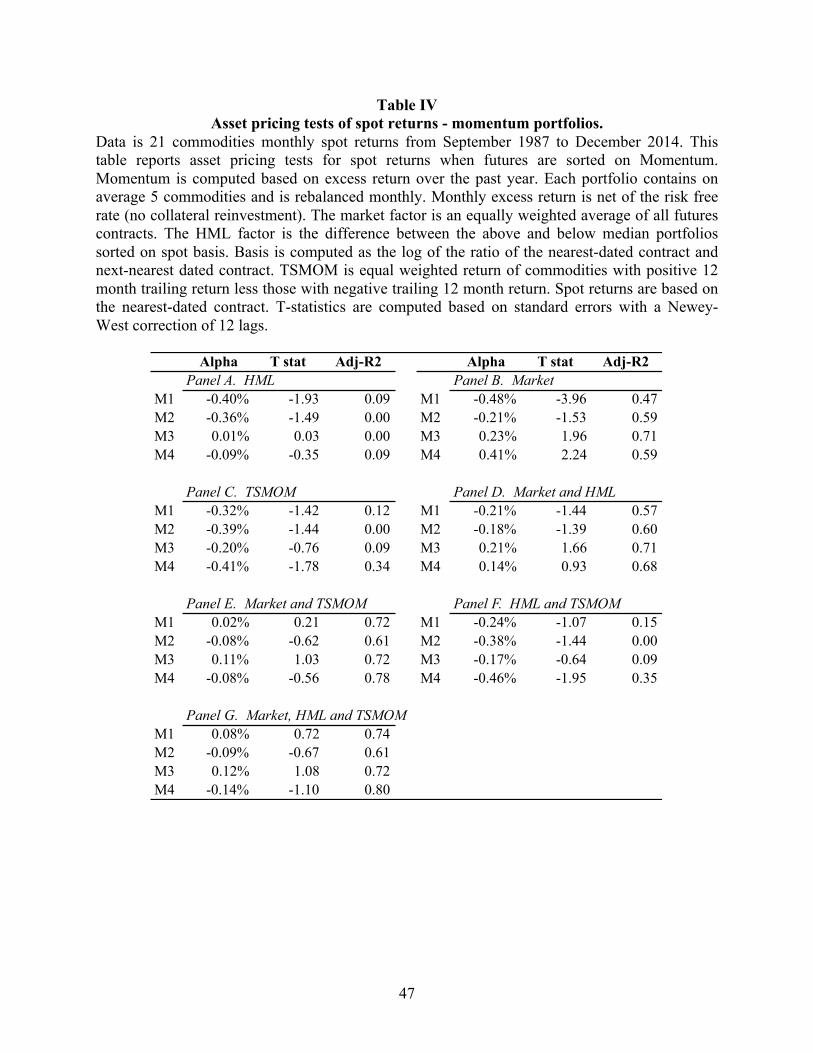
47

Table IV Asset pricing tests of spot returns - momentum portfolios.

Data is 21 commodities monthly spot returns from September 1987 to December 2014. This table reports asset pricing tests for spot returns when futures are sorted on Momentum. Momentum is computed based on excess return over the past year. Each portfolio contains on average 5 commodities and is rebalanced monthly. Monthly excess return is net of the risk free rate (no collateral reinvestment). The market factor is an equally weighted average of all futures contracts. The HML factor is the difference between the above and below median portfolios sorted on spot basis. Basis is computed as the log of the ratio of the nearest-dated contract and next-nearest dated contract. TSMOM is equal weighted return of commodities with positive 12 month trailing return less those with negative trailing 12 month return. Spot returns are based on the nearest-dated contract. T-statistics are computed based on standard errors with a Newey-West correction of 12 lags.

Alpha T stat Adj-R2 Alpha T stat Adj-R2Panel A. HML Panel B. Market

M1 -0.40% -1.93 0.09 M1 -0.48% -3.96 0.47M2 -0.36% -1.49 0.00 M2 -0.21% -1.53 0.59M3 0.01% 0.03 0.00 M3 0.23% 1.96 0.71M4 -0.09% -0.35 0.09 M4 0.41% 2.24 0.59

Panel C. TSMOM Panel D. Market and HMLM1 -0.32% -1.42 0.12 M1 -0.21% -1.44 0.57M2 -0.39% -1.44 0.00 M2 -0.18% -1.39 0.60M3 -0.20% -0.76 0.09 M3 0.21% 1.66 0.71M4 -0.41% -1.78 0.34 M4 0.14% 0.93 0.68

Panel E. Market and TSMOM Panel F. HML and TSMOMM1 0.02% 0.21 0.72 M1 -0.24% -1.07 0.15M2 -0.08% -0.62 0.61 M2 -0.38% -1.44 0.00M3 0.11% 1.03 0.72 M3 -0.17% -0.64 0.09M4 -0.08% -0.56 0.78 M4 -0.46% -1.95 0.35

Panel G. Market, HML and TSMOMM1 0.08% 0.72 0.74M2 -0.09% -0.67 0.61M3 0.12% 1.08 0.72M4 -0.14% -1.10 0.80

48

Table V Asset pricing tests of term premia - basis portfolios.

Data is 21 commodities two-, four- and six-month term premia from September 1987 to December 2014. This table reports asset pricing tests for term premia with holding period returns of two-, four-, and six-months when futures are sorted on basis computed at sequentially longer dated maturities. Basis is computed as the log of the ratio of the nearest-dated contract and longer dated contract (two-, four- or six-months later). Each portfolio contains on average 5 commodities and is rebalanced monthly. Hterm is the equal weighted average of top quartile portfolio of two-, four-, and six-month calendar spread returns. Lterm is the same but the bottom quartile. The HML factor is the difference between Hterm and Lterm. T-statistics are computed based on standard errors with a Newey-West correction of 12 lags.

HML (term) Factor Hterm and Lterm

Alpha T stat Adj-R2 Alpha T stat Adj-R2

B1 0.16% 3.44 0.20 B1 0.02% 1.00 0.57B2 0.09% 2.48 0.10 B2 0.01% 0.34 0.34B3 0.08% 2.31 0.07 B3 0.02% 0.56 0.20B4 0.26% 4.53 0.39 B4 0.08% 2.65 0.66

B1 0.22% 3.11 0.24 B1 -0.02% -0.58 0.68B2 0.14% 3.41 0.15 B2 0.00% 0.15 0.42B3 0.06% 1.41 0.08 B3 -0.04% -1.00 0.23B4 0.31% 3.84 0.41 B4 0.03% 0.65 0.71

B1 0.32% 3.57 0.26 B1 0.01% 0.21 0.67B2 0.14% 2.87 0.14 B2 -0.03% -0.69 0.39B3 0.03% 0.62 0.06 B3 -0.10% -2.32 0.24B4 0.38% 3.93 0.43 B4 0.04% 0.66 0.71

Panel A. Two Month Term Premia

Panel B. Four Month Term Premia

Panel C. Six Month Term Premia

49

Table VI Tests for redundancy among factors in factor model

Data is 21 commodities monthly spot returns from September 1987 to December 2014. This table reports results from regressions of the factors on each other to test for redundancy. If a factor has an intercept no different from zero, it is redundant. The momentum factor (MOM) is a cross-sectional momentum factor not used in our final model. It is defined as the top quartile portfolio less the bottom quartile portfolio of commodities sorted on the previous twelve months of spot returns. The market factor (MKT) is an equally weighted average of all futures contracts. The HML factor is the difference between the above and below median portfolios sorted on spot basis. Basis is computed as the log of the ratio of the nearest-dated contract and next-nearest dated contract. TSMOM is equal weighted return of commodities with positive 12 month trailing return less those with negative trailing 12 month return. Hterm is the equal weighted average of top quartile portfolio of two-, four-, and six-month calendar spread returns. Lterm is the same but the bottom quartile. Spot returns are based on the nearest-dated contract. T-statistics are computed based on standard errors with a Newey-West correction of 12 lags.

Dependent Variable Intercept t-statistic Adj-R2 Independent Variables

MOM 0.08% 0.33 0.02 MKT, HML and TSMOMTSMOM 0.61% 3.31 0.19 MKT and HMLHML 0.31% 1.86 0.15 MKT and TSMOM

Dependent Variable Intercept t-statistic Adj-R2 Independent Variables

MOM -0.01% -0.03 0.02 MKT, HML, TSMOM, Hterm, Lterm

TSMOM 0.63% 3.06 0.18 MKT, HML, Hterm, Lterm

HML 0.12% 0.76 0.40 MKT, TSMOM, Hterm, Lterm

Dependent Variable Intercept t-statistic Adj-R2 Independent Variables

Hterm 0.17% 3.30 0.15 MKT, HML and TSMOMLterm 0.15% 3.11 0.29 MKT, HML and TSMOMHterm 0.12% 3.08 0.19 MKT, HML and TSMOM, Lterm

Lterm 0.12% 3.04 0.33 MKT, HML and TSMOM, Hterm

50

Table VII Summary statistics of commodity trading funds

This table presents the time-series averages of cross-sectional statistics from December of 2006 through December of 2014. Standard deviation, skewness and kurtosis are also computed on excess returns. These excess returns are the futures contract return without adding in any return from collateral reinvestment and so are net of the risk free rate. Excess kurtosis is computed kurtosis minus 3, which is the kurtosis of the normal distribution. The Jarqua-Bera p-value tests the null hypothesis that skewness and excess kurtosis are zero. The Breusch-Pagan Tests for heteroskedasticity and the Ljung-Box tests for autocorrelation. The percent of p-values less than 0.10 is displayed for each. Track record length is in months. Total number of unique funds spans the entire sample. Average number of funds is per month and average amount of assets under management in millions of US dollars. Live funds are those in operation at the end of the sample, December of 2014. Dead funds are those that stopped reporting prior to the data. Statistics are documented for three groups of CTA fund manager categories: energy traders, agricultural traders and metal traders..

Mean Excess Return

Median Excess Return

Standard Deviation Skewness

Excess Kurtosis

Jarque-Bera p values < 0.1

Breusch-Pagan p values < 0.1

Ljung-Box p values

< 0.1

Average Track

Record Length

(Months)

Total Number

of unique funds

Average Number of funds per

month

Average AUM ($M)

Number of observations

All Funds 0.35% 0.25% 4.25% 0.21 2.14 53.55% 14.21% 19.67% 65 183 122 726$ 11,859

By CategoryEnergy 0.51% 0.26% 4.07% 0.59 2.69 66.67% 6.67% 13.33% 74 15 11 79$ 1,104 Agricultural 0.17% -0.13% 5.93% 0.63 3.77 69.44% 13.89% 2.78% 71 36 26 31$ 2,542 Metals 0.39% 0.36% 3.81% 0.05 1.63 47.73% 15.15% 25.00% 62 132 85 989$ 8,213

By Current StatusLive funds 0.61% 0.33% 4.25% 0.40 2.12 93 53 51 2,123 4,954 Dead funds 0.25% 0.22% 4.25% 0.13 2.14 53 130 71 157 6,905

51

Table VIII Statistical significance of the best and worst funds' performance.

This table reports results on the nonparametric bootstrap of distribution is done as in Kosowski, Naik, and Teo (2007). The first row reports the t-statistic of alpha based on heteroskedasticity and autocorrelation consistent standard errors. The second row reports the p-value of that t-statistic based on the bootstrapped distribution. Row 3 reports the ranked alpha based on the commodity four-factor model of Market, HML, Hterm and Lterm. Row 4 reports the p-value for alpha based on the bootstrapped distribution. Note that Row 1 and Row 3 are not necessarily in the same order. The first column is the bottom-ranked fund, the last column the top. In between, we report the bottom and top 1st, 3rd, 5th, and 10th percentiles of the distribution. The sample is from December of 2006 through December 2014.

Bottom 1% 3% 5% 10% 10% 5% 3% 1% TopT stat of alpha -2.37 -2.34 -2.13 -1.88 -1.41 1.53 1.81 2.27 3.29 6.00p-value(bootstrapped) 1.39% 1.48% 2.10% 3.34% 7.50% 5.35% 3.14% 1.30% 0.18% 0.01%

Alpha -4.09% -2.67% -2.08% -1.49% -0.92% 0.94% 1.46% 1.69% 3.29% 4.27%p-value(bootstrapped) 0.04% 0.20% 0.48% 1.24% 3.87% 3.82% 1.48% 1.02% 0.10% 0.03%

52

Table IX Portfolios of funds formed on the t-statistic of alpha (OLS)

This table reports out-of-sample performance of portfolios sorted on the OLS-estimated t-statistic of alpha over the period January 2009 and December of 2014. The in-sample period starts in December 2006. Performance metrics include annualized alpha, t-statistic of alpha, standard deviation, and Sharpe Ratio. Quintile I is the highest performing, Quintile V is the lowest performing. The final row reports the spread. Below that are the pooled sample results (“Overall”). Panel A presents results for the first 12 months post-formation, Panel B reports results for the subsequent 12 months (months 13-24 post-formation). T-statistics are computed based on standard errors with a Newey-West correction of 12 lags.

Panel A. 12 Months Post-Formation

Quintiles Alpha T-statI 2.53% 3.31

II 0.70% 0.32III 0.20% 0.12IV -0.07% -0.06V -1.94% -1.65

I-V 4.47% 3.15Overall 0.28% 0.36

Panel B. 13-24 Months Post-Formation

Quintiles Alpha T-statI 0.61% 0.35

II 0.59% 0.33III 2.01% 1.38IV -1.42% -0.77V -0.94% -0.58

I-V 1.55% 0.72

Std DevSharpe Ratio

3.64% 1.12 5.48% 0.08 4.99% 0.38 5.35% 0.23 5.04% (0.26) 5.90% 0.91

3.33% 0.38

Std DevSharpe Ratio

4.72% 0.34 3.98% 0.18 4.88% 0.69 4.88% 0.26 4.13% 0.27 4.76% 0.11

53

Table IX Portfolios of funds formed on the t-statistic of alpha (Bayesian SURA)

This table reports out-of-sample performance of portfolios sorted on the Bayesian SURA-estimated t-statistic of alpha over the period January 2009 and December of 2014. The in-sample period starts in December 2006. Performance metrics include annualized alpha, t-statistic of alpha, standard deviation, and Sharpe Ratio. Quintile I is the highest performing, Quintile V is the lowest performing. The final row reports the spread. Below that are the pooled sample results (“Overall”). Panel A presents results for the first 12 months post-formation, Panel B reports results for the subsequent 12 months (months 13-24 post-formation). T-statistics are computed based on standard errors with a Newey-West correction of 12 lags.

Panel A. 12 Months Post-Formation

Quintiles Alpha T-statI 2.31% 1.72

II 1.41% 0.78III 0.25% 0.16IV -0.97% -0.84V -1.67% -1.91

I-V 3.98% 2.84Overall 0.27% 0.34

Panel B. 13-24 Months Post-Formation

Quintiles Alpha T-statI 1.34% 0.87

II 0.84% 0.72III -0.24% -0.18IV -0.26% -0.28V -0.93% -0.62

I-V 2.27% 1.13

Std DevSharpe Ratio

4.72% 0.92 5.11% 0.31 5.78% 0.37 4.41% 0.08 3.94% (0.51) 5.81% 1.09

3.33% 0.38

Std DevSharpe Ratio

4.76% 0.61 4.39% 0.46 5.52% 0.29 3.62% 0.29 3.32% 0.12 4.09% 0.61

54

Table XI Portfolios of funds formed on the t-statistic of alpha (non-metals)

This table reports out-of-sample performance of portfolios of non-metal CTAs sorted on estimated t-statistic of alpha over the period January 2009 and December of 2014. The in-sample period starts in December 2006. Performance metrics include annualized alpha, t-statistic of alpha, standard deviation, and Sharpe Ratio. Quintile I is the highest performing, Quintile V is the lowest performing. The final row reports the spread. Below that are the pooled sample results (“Overall”). Panel A presents results for the OLS estimates, Panel B reports results for the Bayesian SURA estimates. T-statistics are computed based on standard errors with a Newey-West correction of 12 lags.

Panel A. OLS

Quintiles Alpha T-stat Std DevSharpe Ratio

I 4.08% 3.49 5.19% 1.02 II 5.49% 1.50 10.95% 0.59 III 0.71% 0.33 6.68% 0.31 IV -0.07% -0.02 7.42% 0.16 V -3.48% -1.65 6.90% (0.45)

I-V 7.56% 4.11 6.82% 1.24 Overall 1.34% 0.91 5.00% 0.47

Panel B. Bayesian SUR

Quintiles Alpha T-stat Std DevSharpe Ratio

I 2.76% 1.89 6.09% 0.59 II 4.66% 1.79 7.10% 0.89 III 2.53% 0.76 9.35% 0.40 IV 0.98% 0.39 8.15% 0.30 V -4.26% -2.30 7.11% (0.60)

I-V 7.02% 3.25 7.80% 1.01 Overall 1.34% 0.91 4.98% 0.47

55

Table XII Portfolios of funds formed on the t-statistic of alpha (metals)

This table reports out-of-sample performance of portfolios of Metals CTAs sorted on estimated t-statistic of alpha over the period January 2009 and December of 2014. The in-sample period starts in December 2006. Performance metrics include annualized alpha, t-statistic of alpha, standard deviation, and Sharpe Ratio. Quintile I is the highest performing, Quintile V is the lowest performing. The final row reports the spread. Below that are the pooled sample results (“Overall”). Panel A presents results for the OLS estimates, Panel B reports results for the Bayesian SURA estimates. T-statistics are computed based on standard errors with a Newey-West correction of 12 lags.

Panel A. OLS

Quintiles Alphat-stat alpha StDev Sharpe

I 2.80% 2.78 5.19% 1.02 II 0.36% 0.20 10.95% 0.59 III -1.09% -0.46 6.68% 0.31 IV -0.98% -0.69 7.42% 0.16 V -1.89% -1.11 6.90% (0.45)

I-V 4.69% 2.59 6.82% 1.24 Overall -0.16% -0.16 4.27% 0.18

Panel B. Bayesian SUR

Quintiles Alphat-stat alpha StDev Sharpe

I 2.72% 1.63 6.09% 0.59 II 0.77% 0.34 7.10% 0.89 III -1.97% -1.10 9.35% 0.40 IV -0.04% -0.03 8.15% 0.30 V -1.96% -1.91 7.11% (0.60)

I-V 4.68% 2.39 7.80% 1.01 Overall -0.10% -0.09 4.28% 0.19

56

Table XIII

The effect of biased data: adjusted data vs full sample This table reports out-of-sample Bayesian SURA estimated performance of the quintiles portfolios for the period between January of 1996 and December of 2014 and January of 2009 to December of 2014. Only alpha and the t-statistic of alpha are reported (note that 2009-2014 results duplicate Table VIII and are replicated for ease of comparison). The final two columns are simply the difference in values for the two sample periods displayed.

Quintiles Alpha T-stat Alpha T-stat Alpha T-statI 4.89% 3.02 2.31% 1.72 2.57% 1.31II 4.09% 2.93 1.41% 0.78 2.68% 2.16III 3.56% 2.31 0.25% 0.16 3.31% 2.15IV 2.12% 1.62 -0.97% -0.84 3.09% 2.46V -0.23% -0.17 -1.67% -1.91 1.45% 1.73I-V 5.11% 3.65 3.98% 2.84 1.13% 0.82

1996-2014 2009-2014 Difference