performance analysis on free-piston linear expander
TRANSCRIPT
UNF Digital Commons
UNF Graduate Theses and Dissertations Student Scholarship
2017
Performance analysis on Free-piston linearexpanderFurkan KodakogluUniversity of North Florida
This Master's Thesis is brought to you for free and open access by theStudent Scholarship at UNF Digital Commons. It has been accepted forinclusion in UNF Graduate Theses and Dissertations by an authorizedadministrator of UNF Digital Commons. For more information, pleasecontact Digital Projects.© 2017 All Rights Reserved
Suggested CitationKodakoglu, Furkan, "Performance analysis on Free-piston linear expander" (2017). UNF Graduate Theses and Dissertations. 766.https://digitalcommons.unf.edu/etd/766

PERFORMANCE ANALYSIS ON FREE-PISTON LINEAR EXPANDER
by
Furkan Kodakoğlu
A thesis submitted to the Department of Mechanical Engineering
In partial fulfillment of the requirements for the degree of
Masters of Science in Mechanical Engineering
UNIVERSITY OF NORTH FLORIDA
COLLEGE OF COMPUTING, CONSTRUCTION, AND ENGINEERING
August, 2017
Unpublished work © Furkan Kodakoğlu

ii
Certificate of Approval
The thesis “Performance analysis on free-piston linear expander” submitted by Furkan Kodakoğlu
in partial fulfillment of the requirements for the degree of Master of Science in Mechanical
Engineering has been
Approved by the thesis committee: Date Dr. John Nuszkowski Thesis Advisor and Committee Chairperson Dr. Stephen Stagon Dr. Gregory Thompson Accepted for the School of Engineering: Dr. Murat Tiryakioğlu Director of the School Accepted for the College of Computing, Engineering, and Construction: Dr. Mark Tumeo Dean of the College Accepted for the University: Dr. John Kantner Dean of the Graduate School

iii
Acknowledgements
First, I would like to express my deepest gratitude to my advisor Dr. John Nuszkowski for
giving me the opportunity to work on this project under his supervision. I had a golden
learning experience by benefiting from your professional knowledge, guidance and
experimentalist skills throughout my study.
I am also grateful to Dr. Gregory Thompson and Dr. Stephen Stagon for their interests in
this study and accepting to be on my thesis committee.
I would like to thank Dr. Murat Tiryakioğlu for his valuable and motivational support. His
encouragement has given me a priceless power. My appreciation is extended to my friend
Aygun Baltaci, a former electrical engineering student of UNF, for helping me through the
adapting process from the beginning of my USA journey. I wish him great successes during
his master’s studies in the Technical University of Munich and after his graduation.
I would also like to thank Dr. Alexandra Schonning for keeping her door always open to
me. In addition, a special thanks goes to the great staff of UNF, especially Jean Loos for
giving me the chance to learn very useful skills in the machining stages of my study. She
is an excellent teaching specialist.
The completion of this research project would not be possible without the constant support
of my family. I thank my father and my mother for being my personal guidance and raising
me to this day, and my brother for always being there whenever I need him.

iv
Table of Contents
Certificate of Approval ....................................................................................................... ii
Acknowledgements ............................................................................................................ iii
Table of Contents ............................................................................................................... iv
List of Figures ................................................................................................................... vii
List of Tables .......................................................................................................................x
List of Abbreviations ........................................................................................................ xii
List of Symbols ................................................................................................................ xiii
Abstract ..............................................................................................................................xv
1 Introduction ..............................................................................................................1
2 Low Temperature Energy Recovery ........................................................................4
2.1 Carnot Cycle ...........................................................................................................4
2.2 Kalina Cycle ...........................................................................................................6
2.3 Transcritical CO2 Cycle .........................................................................................8
2.4 Stirling Engine........................................................................................................9
2.5 Thermoelectric Generators ...................................................................................11
2.6 Organic Rankine Cycle ........................................................................................12
2.6.1 Cycle Configurations ......................................................................................13
2.6.2 Working Fluids ...............................................................................................15
2.6.3 Irreversibilities ................................................................................................18

v
2.6.4 Cycle Improvements .......................................................................................19
2.6.5 Applications ....................................................................................................20
2.7 Comparison of Low Temperature Energy Recovery Methods ............................22
2.8 Expansion Machines ............................................................................................22
2.8.1 Turbomachinery .............................................................................................23
2.8.2 Scroll Expander ..............................................................................................26
2.8.3 Screw Expander ..............................................................................................29
2.8.4 Rotary Vane Expander ...................................................................................32
2.8.5 Gerotor Expander ...........................................................................................33
2.8.6 Reciprocating Piston Expander ......................................................................35
2.8.7 Rotary Piston Expander ..................................................................................37
2.8.8 Free-Piston Linear Expander ..........................................................................39
2.8.9 Comparison of Expanders ..............................................................................44
3 Experimental Setup and Analysis ..........................................................................47
3.1 Design...................................................................................................................48
3.1.1 Previous Design ..............................................................................................48
3.1.2 Modifications ..................................................................................................50
3.2 Measurement Devices ..........................................................................................57
3.2.1 Temperature Measurements ...........................................................................58
3.2.2 Pressure Measurements ..................................................................................58

vi
3.2.3 Flow Rate Measurement .................................................................................59
3.2.4 LabJack U12 ...................................................................................................60
3.3 Thermodynamic Analysis ....................................................................................61
3.3.1 Propagation of Error .......................................................................................67
4 Results and Discussion ..........................................................................................68
4.1 Different Inlet Air Pressures ................................................................................69
4.2 Different Inlet Air Temperatures..........................................................................74
4.3 Different Resistance Magnitudes .........................................................................80
5 Conclusion .............................................................................................................87
6 Future Work ...........................................................................................................90
References ..........................................................................................................................91
Appendix A ........................................................................................................................98

vii
List of Figures
Figure 2.1: Carnot Efficiency as a Function of Heat Source Temperature (TH), T0=25 °C 5
Figure 2.2: Component Diagram of a Simplified Kalina Cycle ......................................... 6
Figure 2.3: Comparison of Isentropic T-S Diagrams of Rankine (Left) and Kalina Cycle
(Right) ................................................................................................................................. 7
Figure 2.4: R123 (left) vs CO2 (right) Heat Transfer.......................................................... 8
Figure 2.5: (a) T-s and (b) P-ѵ Diagrams and (c) Demonstration of an Ideal Stirling Cycle
........................................................................................................................................... 10
Figure 2.6: The Arrangement of the P and N-type Semiconductors in a TEG ................. 12
Figure 2.7: Component Diagram of a Basic Organic Rankine Cycle ............................... 14
Figure 2.8: Regenerative Configuration of ORC .............................................................. 15
Figure 2.9: T-s Diagrams of Different Type of Organic Working Fluids ........................ 16
Figure 2.10: Irreversibility-Turbine Inlet Pressure Relation for Different Working Fluids
at Constant Inlet Temperature ........................................................................................... 19
Figure 2.11: Turbine Types: Impulse Turbine (left), Reaction Turbine (Middle), and Radial
Inflow Turbine (right) ....................................................................................................... 23
Figure 2.12: Centripetal (left) and Centrifugal (right) Turbines ....................................... 24
Figure 2.13: Working Process of a Scroll Expander......................................................... 27
Figure 2.14: Flank and Radial Leakages........................................................................... 28
Figure 2.15: Working Processes of a Twin Screw Expander ........................................... 30
Figure 2.16: Working Mechanism of a Single Screw Expander ...................................... 30
Figure 2.17: Design and Working Processes of a Rotary Vane Expander ....................... 32
Figure 2.18: Working Processes of a Gerotor Expander .................................................. 34

viii
Figure 2.19: Operation of a Reciprocating Piston Expander ............................................ 35
Figure 2.20: Intake, Expansion, and Discharge Processes of a Rolling Piston Expander 38
Figure 2.21: Cut-away View of a FPLE ........................................................................... 41
Figure 3.1: Schematic of the Test Bench .......................................................................... 48
Figure 3.2: The Piston with O-rings (O-rings in red color) .............................................. 51
Figure 3.3: 2-D Drawing of the Washer Cap with Dimensions ........................................ 53
Figure 3.4: The Flange of the Cylinder with O-ring and the Spring-Washer Cap Assembly
........................................................................................................................................... 54
Figure 3.5: FPLE Modified Experimental Setup; 1) FPLE, 2) Heater, 3) Pressure Gauge,
4) Flow Meter, 5) Control Panel, 6) Flow Control Valve, 7) Resistor Bank, 8) LabJack for
Voltage Measurements, 9) LabJack for Temperature and Pressure Measurements, 10) C-
Clamp for Table, 11) L-Clamp for Expander Support, 12) Pipe Clamp for FPLE, 13) Inlet
Air Temperature Thermocouple ....................................................................................... 57
Figure 4.1: Determination of Steady State Region ........................................................... 69
Figure 4.2: Variation in Expander Frequency for Different Inlet Air Pressures .............. 72
Figure 4.3: Efficiencies at Different Inlet Air Pressures................................................... 73
Figure 4.4: The Average RMS Voltages at Different Inlet Air Pressures ........................ 73
Figure 4.5: Actual Expander Work and Irreversibility Variations in Different Inlet Air
Pressures ........................................................................................................................... 74
Figure 4.6: Variation of Expander Frequency for Different Inlet Air Temperatures ....... 77
Figure 4.7: The Average RMS Voltages at Different Inlet Air Temperatures ................. 77
Figure 4.8: Efficiencies at Different Inlet Air Temperatures ............................................ 79

ix
Figure 4.9: Actual Expander Work and Irreversibility Variations in Different Inlet Air
Temperatures..................................................................................................................... 80
Figure 4.10: The Average RMS Voltages at Different Resistance Magnitudes ............... 83
Figure 4.11: Variation of Expander Frequency for Different Resistance Magnitudes ..... 83
Figure 4.12: Efficiencies at Different Resistance Magnitudes ......................................... 85
Figure 4.13: Actual Expander Work and Irreversibility Variations in Different Resistance
Magnitudes ........................................................................................................................ 86

x
List of Tables
Table 1.1: World Primary Energy Demand by Source ....................................................... 2
Table 2.1: Working Fluids for Low Grade Heat Sources ................................................. 18
Table 3.1: Chamber-to-Chamber Working Processes ...................................................... 49
Table 3.2: Spring Technical Specifications ...................................................................... 52
Table 3.3: Heater Technical Specifications ...................................................................... 55
Table 3.4: Technical Specifications of Insulation Material .............................................. 55
Table 3.5: Technical Specifications of the Thermocouples .............................................. 58
Table 3.6: Specifications of the Pressure Gauge .............................................................. 59
Table 3.7: Technical Specifications of the Pressure Sensors ............................................ 59
Table 3.8: Technical Specifications of the Flow Meter .................................................... 60
Table 3.9: Analog Inputs (AI0 – AI7) Technical Specifications of the LabJack U12 ...... 61
Table 3.10: Design of Experiments .................................................................................. 66
Table 4.1: Experimental Thermodynamic Data Collected at Different Inlet Air Pressures
........................................................................................................................................... 70
Table 4.2: The FPLE Performance Summary at Different Inlet Air Pressures ................ 71
Table 4.3: Experimental Thermodynamic Data Collected at Different Inlet Air
Temperatures..................................................................................................................... 75
Table 4.4: The FPLE Performance Summary at Different Inlet Air Temperatures.......... 76
Table 4.5: Experimental Thermodynamic Data Collected at Different Resistance
Magnitudes ........................................................................................................................ 81
Table 4.6: The FPLE Performance Summary at Different Resistance Magnitudes ......... 82

xi
Table A.1: Standard Deviation Results of the Calculated Parameters for Experimental Set
1......................................................................................................................................... 98
Table A.2: Standard Deviation Results of the Calculated Parameters for Experimental Set
2......................................................................................................................................... 98
Table A.3: Standard Deviation Results of the Calculated Parameters for Experimental Set
3......................................................................................................................................... 99
xii
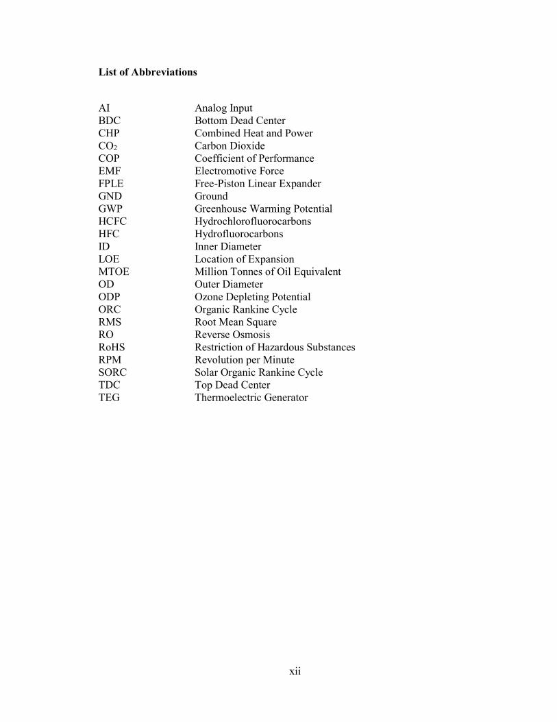
List of Abbreviations
AI Analog Input BDC Bottom Dead Center CHP Combined Heat and Power CO2 Carbon Dioxide COP Coefficient of Performance EMF Electromotive Force FPLE Free-Piston Linear Expander GND Ground GWP Greenhouse Warming Potential HCFC Hydrochlorofluorocarbons HFC Hydrofluorocarbons ID Inner Diameter LOE Location of Expansion MTOE Million Tonnes of Oil Equivalent OD Outer Diameter ODP Ozone Depleting Potential ORC Organic Rankine Cycle RMS Root Mean Square RO Reverse Osmosis RoHS Restriction of Hazardous Substances RPM Revolution per Minute SORC Solar Organic Rankine Cycle TDC Top Dead Center TEG Thermoelectric Generator

xiii
List of Symbols
��𝑔𝑒𝑛 Entropy Generation ��𝑒,𝑎𝑣𝑔 Average Electrical Power Output ��𝑜𝑢𝑡,𝑎 Rate of Actual Work Output ��𝑜𝑢𝑡,𝑠 Rate of Isentropic Work Output 𝑚𝑎 Mass Flow Rate of Air E𝑐𝑣 Total Internal Energy in Control Volume m𝑐𝑣 Mass in Control Volume η𝐶𝑎𝑟𝑛𝑜𝑡 Carnot Efficiency �� Rate of Heat Transfer 𝑅𝑎 Gas Constant of Air 𝑅𝑒𝑞 Equivalent Resistance 𝑇𝑜𝑢𝑡,𝑎 Exit Temperature in Actual Process 𝑇𝑜𝑢𝑡,𝑠 Exit Temperature in Isentropic Process 𝑇𝑠 Temperature of Surroundings �� Volumetric Flow Rate 𝑉𝑅𝑀𝑆 RMS Voltage 𝑉𝑑 Displacement Volume �� Rate of Work 𝑐𝑝 Specific Heat �� Mass Flow Rate 𝜂𝑐 Mechanical-Electrical Conversion Efficiency 𝜂𝑠 Isentropic Efficiency 𝜌𝑎 Density of Air ∆𝑇 Temperature Gradient ∆𝑉 Voltage Differential ℎ Enthalpy Pcrit Critical Pressure S Entropy T0 Ambient Temperature Tcrit Critical Temperature TH Constant Temperature of High Heat Source TL Constant Temperature of Low Heat Source 𝐷 Diameter 𝐼 Irreversibility 𝑉 Velocity 𝑓 Frequency 𝑘 Specific Heat Ratio 𝑛 Shaft Speed 𝑡 Time 𝑣 Tip Speed 𝑧 Height Level 𝛼 Seebeck Coefficient

xiv
𝜆 Volumetric Efficiency 𝜎 Standard Deviation

xv
Abstract
The growing global demand for energy and environmental implications have created a need
to further develop the current energy generation technologies (solar, wind, geothermal,
etc.). Recovering energy from low grade energy sources such as waste heat is one of the
methods for improving the performance of thermodynamic cycles. The objective of this
work was to achieve long-term steady state operation of a Free-Piston Linear Expander
(FPLE) and to compare the FPLE with the currently existing expander types for use in low
temperature energy recovery systems. A previously designed FPLE with a single piston,
two chambers, and linear alternator was studied and several modifications were applied on
the sealing and over expansion. An experimental test bench was developed to measure the
inlet and outlet temperatures, inlet and outlet pressures, flow rate, and voltage output. A
method of thermodynamic analysis was developed by using the first and second law of
thermodynamics with air as the working fluid. The experimental tests were designed to
evaluate the performance of the FPLE with varying parameters of inlet air pressure, inlet
air temperature, and electrical resistance. The initial and steady-state operation of the FPLE
were successfully achieved. An uncertainty analysis was conducted on the measured values
to determine the accuracies of the calculated parameters. The trends of several output
parameters such as frequency, average root mean square (RMS) voltage, volumetric
efficiency, electrical-mechanical conversion efficiency, isentropic efficiency,
irreversibility, actual expander work, and electrical power were presented. Results showed
that the maximum expander frequency was found to be 44.01 Hz and the frequency tended
to increase as the inlet air pressure increased. The FPLE achieved the maximum isentropic

xvi
efficiency of 21.5%, and produced maximum actual expander work and electrical work of
75.13 W and 3.302 W, respectively.
1
1 Introduction
A great amount of energy that the planet earth contains and “the unlimited” energy
that the sun keeps providing shows the energy potential that can be reached. The human
race has started to become more capable of using this potential in order to improve the
quality of human life. However, “usable” energy has always been an essential need. Since
the industrial revolution, the need for energy has been rapidly increasing mainly due to
industrialization, and the changes in transportation and manufacturing processes around
the world. In conjunction with this revolution, the power of heat was discovered and
replaced the power need that was met by means of human- or/and animal-based methods.
After the invention of the steam engine, by James Watt [1], in the 1800s and the technology
developments that followed, society entered into a "technology era." This demand on
technology that relies on mechanical or electrical power ensures the continued significance
of the global energy supply.
Unfortunately, the vast majority of the growing global energy demand (81.6%) is
met by fossil fuels [2]. Table 1.1 presents the share distribution of the world global energy
demand by source. The combustion of the fossil fuels consisting of hydrocarbon
components produces several pollutants such as carbon dioxide, sulfur dioxide, nitric
oxides, carbon monoxide, and partly unburned particulates. These byproducts are
responsible for several global threats, e.g. global warming, acid rain, ocean acidification,
and environmental pollution that have hazardous effects for all living beings [3,23].

2
Table 1.1: World Primary Energy Demand by Source [2]
MTOE Percent %
Coal 3 773 28.9
Oil 4 108 31.4
Gas 2 787 21.3
Nuclear 674 5.2
Hydro 300 2.3
Bioenergy 1 300 9.9
Other renewables 127 1
Total 13 069 100
The percentages above do not represent the total amount of energy that is converted
into usable power. The efficiency of power generation, at this point, becomes the crucial
consideration. Efficiency is defined by the ratio of the energy obtained to the energy input
and is usually expressed in percentages. As is the case with all processes, energy
conversion from chemical to electrical power has inherent losses and limitations. Heat and
friction losses can be considered as the main inherent losses. The Carnot efficiency, which
is the theoretical maximum efficiency of any thermodynamic cycle, is one of the
limitations.
The primary energy consumption of the U.S. is approximately 100 quadrillion [Btu]
(approximately 2521 MTOE, or 1.06 X 10²⁰ Joules) each year, and 20% of this total
amount, 20 quadrillion Btu, is provided by coal. In addition to this, 92% of the coal source
used in the U.S. is converted into electricity power [4]. The average conversion efficiency
of the coal power plants operating in the U.S. is about 34% [5]. These facts indicate that
3
6.26 of the 18.4 quadrillion [Btu] of energy has been converted into electricity and the rest
is released into the environment as waste energy in the U.S. each year. Power generation
from other sources can be assumed to have a similar situation that results in waste energy.
Current global trends clearly show that the demand for fossil fuels will increase
until 2035 [2], thereby forcing us to further develop current energy generation
technologies. In this regard, efficiencies of the current thermodynamic cycle designs also
need to be improved so that the dependence on the fossil fuels can be decreased. Low
temperature heat recovery, in this case, has the potential to utilize the waste energy, thereby
increasing the efficiency of the cycles and helping to reduce air pollution.
The purpose of this work was to investigate the potential of a new type of expander,
the free-piston linear expander (FPLE), outlined by Henry B. Bonar [6]. It was also of
interest to this work to design and build the FPLE to analyze the feasibility of the expander
for advanced low temperature heat recovery systems.

4
2 Low Temperature Energy Recovery
The energy sources can be categorized by their grade and divided into three main
categories, low temperature (<230 °C), medium temperature (230-650 °C), and high
temperature (>650 °C) [7]. There are several methods to utilize the waste energy sources
including the Carnot cycle, the Transcritical CO2 cycle, the Kalina cycle, the Organic
Rankine cycle (ORC), the Stirling engine and the thermoelectric generator (TEG). ORC,
Transcritical CO2 and Kalina cycles can be considered as modifications of the Rankine
cycle. The Stirling engine is a closed reversible cycle that typically resembles the Carnot
cycle. TEGs are devices working on the principle of the Seebeck effect and producing a
voltage from a heat flux [8]. A cursory review and considerations of these methods and the
expanders will be presented.
2.1 Carnot Cycle
The efficiency of any thermodynamic cycle is limited by the second law of
thermodynamics. The low temperature energy recovery cycles are, therefore, limited by
the Kelvin-Planck statement, which is best expressed as follows:
“It is impossible to construct a device that will operate in a cycle and produce no effect
other than the raising of a weight and the exchange of heat with a single reservoir [3].”
Regarding the statement, the Carnot cycle expresses the maximum efficiency that
any heat engine operating between two different, hot and cold, reservoirs can achieve as
follows:

5
η𝐶𝑎𝑟𝑛𝑜𝑡 = 1 −𝑇𝐿
𝑇𝐻
where TH is the constant temperature of the high temperature heat source and TL is the
constant temperature of the low temperature heat rejection sink. Therefore, the Carnot
efficiency, achieved by assuming all the processes are reversible, clearly indicates that the
maximum efficiency of any cycle only depends on the temperatures of the reservoirs. It is
usually not possible to configure the temperature of rejection sink, but the temperature of
the heat source may be pre-adjusted in order to increase the efficiency. Figure 2.1 presents
the Carnot efficiency values as a function of heat source temperature (TH) with the ambient
temperature (T0) value taken as a reference for the rejection sink temperature. It can be
easily seen that the maximum efficiency that can be achieved acts quite sensitive under 700
°C, indicating that the low temperature energy recovery systems will have lower thermal
efficiency.
Figure 2.1: Carnot Efficiency as a Function of Heat Source Temperature (TH), T0=25 °C
0%10%20%30%40%50%60%70%80%90%
0 200 400 600 800 1000 1200
Car
not E
ffic
ienc
y
High Temperature Reservoir [°C]
6
2.2 Kalina Cycle
The Kalina cycle is a thermodynamic cycle invented by Alexander Kalina [9] that
can be considered as a modification of the Rankine cycle. The major difference of this
cycle from the Rankine cycle is the use of a mixture of two different fluids with different
boiling points, most commonly ammonia-water, as a working fluid [10]. The process flow
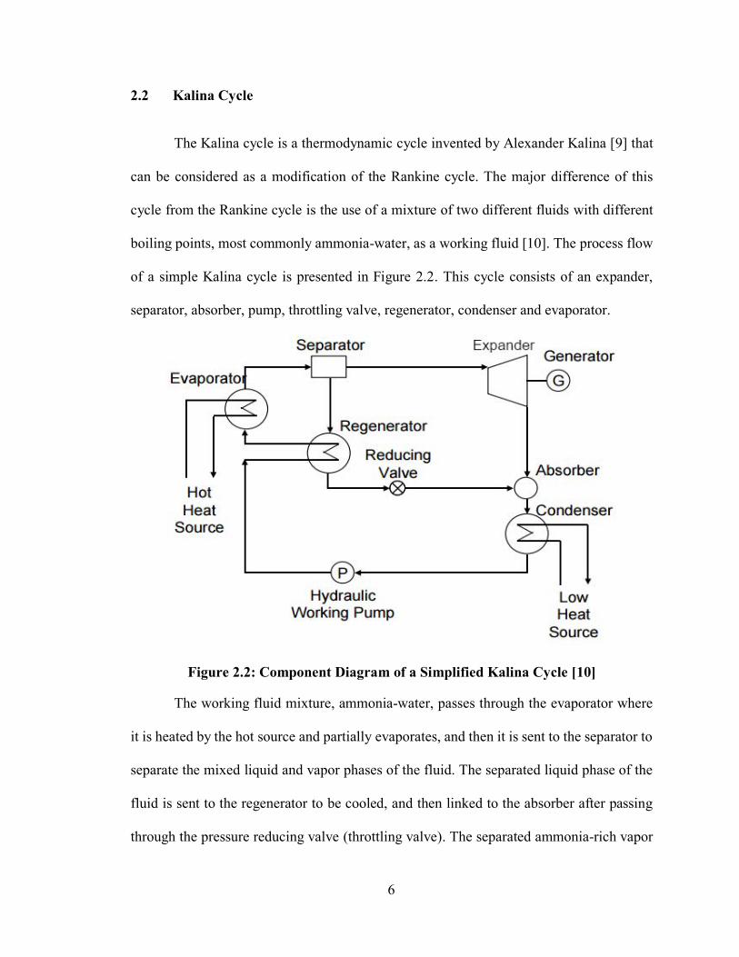
of a simple Kalina cycle is presented in Figure 2.2. This cycle consists of an expander,
separator, absorber, pump, throttling valve, regenerator, condenser and evaporator.
Figure 2.2: Component Diagram of a Simplified Kalina Cycle [10]
The working fluid mixture, ammonia-water, passes through the evaporator where
it is heated by the hot source and partially evaporates, and then it is sent to the separator to
separate the mixed liquid and vapor phases of the fluid. The separated liquid phase of the
fluid is sent to the regenerator to be cooled, and then linked to the absorber after passing
through the pressure reducing valve (throttling valve). The separated ammonia-rich vapor

7
is sent to the expander where it drives the expander and produces the mechanical work that
is, later on, optionally converted into electricity by means of a generator. The vapor stream
leaves the expander as depressurized and cooled fluid and goes into the absorber where the
two streams are accumulated and sent to the condenser. The fluid is, in this step, cooled by
a low heat source and condensed to a complete liquid phase. Afterwards, the pump
pressurizes the condensed liquid and sends the stream to the regenerator where the fluid is
preheated by the separated liquid in the separator. The preheated fluid is, then, sent to the
evaporator where it completes one cycle.
The main goal of this cycle is to, theoretically, increase the average heat absorption
temperature corresponding to the value of TH in the Carnot efficiency (see section 2.1) and
decrease the average heat rejection temperature (TL) by using azeotropic fluids. The feature
of the azeotropic fluids that provides an advantage to the Kalina cycle over the Rankine
cycle is that the temperature of the fluid does not stay constant even during the phase
changes (non-isothermal process). As shown in Figure 2.3, the temperature increases
during evaporation and decreases during condensation achieving the main goal mentioned
above.
Figure 2.3: Comparison of Isentropic T-S Diagrams of Rankine (Left) and Kalina Cycle (Right) [10]
8
The Kalina cycle has been found to have higher performance potential in the heat
recovery applications compared to the usual steam power plants as mentioned by Marston
[11] and Corman et. al. [12]. Hettiarachchi et al. modeled and compared Kalina cycles to
ORCs by using different mixtures of ammonia and water. They obtained higher thermal
efficiencies with the Kalina cycle than the ORC for a given heat supply [13]. Park and
Sontag also performed the second law analysis for the Kalina cycle and steam power cycle
and they stated that the exergy efficiency of the Kalina cycle was 15% higher than that of
the steam power cycle [14].
2.3 Transcritical CO2 Cycle
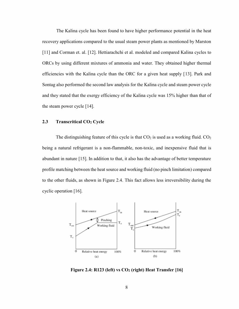
The distinguishing feature of this cycle is that CO2 is used as a working fluid. CO2
being a natural refrigerant is a non-flammable, non-toxic, and inexpensive fluid that is
abundant in nature [15]. In addition to that, it also has the advantage of better temperature
profile matching between the heat source and working fluid (no pinch limitation) compared
to the other fluids, as shown in Figure 2.4. This fact allows less irreversibility during the
cyclic operation [16].
Figure 2.4: R123 (left) vs CO2 (right) Heat Transfer [16]

9
CO2’s relatively low critical temperature (31.10 °C [17]) allows the cycle to operate
close to the triple point, which decreases the amount of work needed to compress the fluid.
The main drawback of this cycle is the fact that the high working pressure of this cycle
must be higher than 73.8 bar in order to achieve supercritical conditions [15]. Therefore,
the capital cost of the system will be higher compared to the subcritical cycles due to the
requirement of thicker piping and pressure vessels [18].
Kinnaly and Nuszkowski emphasize using an expander to recover pressure drop in
a throttling process of the CO2 cycle, which, they believe, can increase the efficiency of
the cycle up to 35% [17,19]. The transcritical cycle could then be competitive with
traditional cycles. Chen et al. conducted a comparative study between a traditional ORC
using R123 as a working fluid and a transcritical CO2 cycle with a 150 °C heat source [20].
From the simulation results, they found that the transcritical CO2 cycle had slightly higher
efficiency over the ORC; confirming that the theoretical efficiency of the CO2 cycle should
have a higher performance than an ORC [20,21].
2.4 Stirling Engine
The Stirling engine is a regenerative cycle invented by Robert Stirling in 1816
(patent no. 4081) [22]. A simple Stirling cycle consists of a cylinder that includes two
pistons in each chamber and a regenerator in the middle, and it comprises four
thermodynamic processes. The main difference between this cycle and the Carnot cycle is
that the Stirling cycle involves two constant-volume regeneration processes, whereas two
isentropic processes take place in the Carnot cycle. The T-s and P-v diagrams of the Stirling
cycle are shown in Figure 2.5 (a) and (b).

10
(a) (b) (c) Figure 2.5: (a) T-s and (b) P-ѵ Diagrams and (c) Demonstration of an Ideal Stirling
Cycle [23]
The thermodynamic processes shown in the diagrams above are:
Isothermal expansion 1-2: heat is added externally to the first chamber at the high
temperature, TH. The piston in the first chamber moves outward isothermally, thereby
increasing the volume and decreasing the pressure.
Constant-volume (isochoric) regeneration (heat removal) 2-3: both pistons move at the
same rate to keep the total volume constant. The fluid moves into the second chamber
while the heat is absorbed by the regenerator in the middle of two chambers. The
temperature of the fluid is, therefore, reduced to TL.
Isothermal compression 3-4: the piston in the second chamber moves inward, thereby
decreasing the volume and increasing the pressure. In the interim, heat is transferred
from the fluid to the heat rejection sink at TL to keep the temperature of the fluid
constant at TL.
Constant-volume (isochoric) regeneration (heat addition) 4-1: both pistons move at the
same rate to keep the total volume constant. The fluid in the second chamber moves

11
into the first chamber while the heat stored by the regenerator is transferred back to the
fluid. This increases the temperature of the fluid to TH and completes one cycle.
The heat addition to the Stirling cycle, demonstrated in Figure 2.5, occurs
externally, which provides an advantage to use any kind of heat source to run the cycle.
However, the external heating also decreases the amount of heat transferred into the system
as mentioned by Tarique [24]. For this cycle, it is recommended to use a working fluid that
has high thermal conductivity, low viscosity, low density and good specific heat capacity.
The working fluids that are most commonly used and give relatively higher performance
are helium and hydrogen [15,16,22,23,24,25,26]. The Stirling engines can be applicable to
low temperature heat recovery systems such as waste energy, solar power, geothermal
sources, etc. [22,25,26].
2.5 Thermoelectric Generators
The thermoelectric generators (TEGs), also called the Seebeck generators, are not
power cycles but devices that generate a voltage differential from a heat flux. TEGs work
on the principle of the Seebeck effect that was discovered by Thomas Seebeck in 1821.
When a temperature gradient is applied to a semiconductor, the heat flowing between the
hot and cold ends will generate an electromotive force (EMF) due to the charge carrier
diffusion and phonon drag [27]. The voltage differential generated via these devices is
defined by:
∆𝑉 = 𝛼∆𝑇
where ∆𝑉 is the voltage differential, ∆𝑇 is the temperature gradient and 𝛼 is the Seebeck
coefficient. The Seebeck coefficient is a property of the conductor and limits the
performance of these devices. A simple TEG is composed of several semiconductors
12
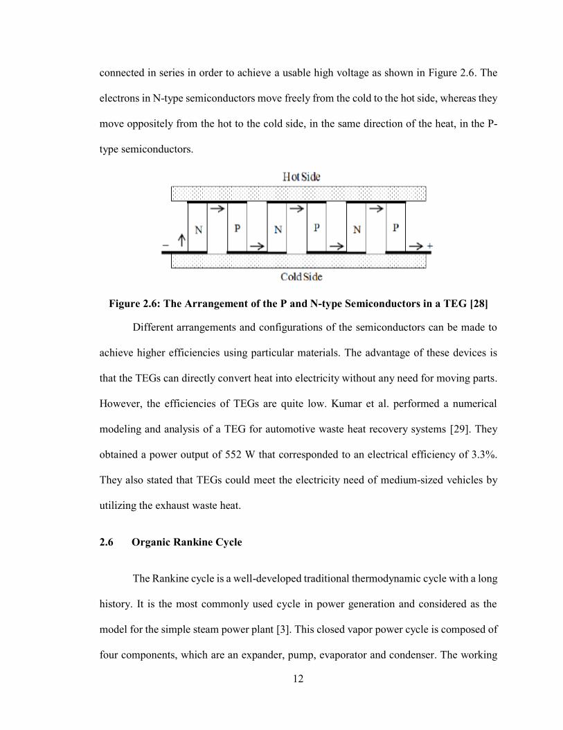
connected in series in order to achieve a usable high voltage as shown in Figure 2.6. The
electrons in N-type semiconductors move freely from the cold to the hot side, whereas they
move oppositely from the hot to the cold side, in the same direction of the heat, in the P-
type semiconductors.
Figure 2.6: The Arrangement of the P and N-type Semiconductors in a TEG [28]
Different arrangements and configurations of the semiconductors can be made to
achieve higher efficiencies using particular materials. The advantage of these devices is
that the TEGs can directly convert heat into electricity without any need for moving parts.
However, the efficiencies of TEGs are quite low. Kumar et al. performed a numerical
modeling and analysis of a TEG for automotive waste heat recovery systems [29]. They
obtained a power output of 552 W that corresponded to an electrical efficiency of 3.3%.
They also stated that TEGs could meet the electricity need of medium-sized vehicles by
utilizing the exhaust waste heat.
2.6 Organic Rankine Cycle
The Rankine cycle is a well-developed traditional thermodynamic cycle with a long
history. It is the most commonly used cycle in power generation and considered as the
model for the simple steam power plant [3]. This closed vapor power cycle is composed of
four components, which are an expander, pump, evaporator and condenser. The working

13
fluid is pressurized via the pump and it is sent to the evaporator where it reaches the
saturated or superheated vapor point. Then, it passes through the expander, generates the
shaft work and is condensed into the liquid phase by a cooling source before returning to
the pump.
The usual working fluid used in Rankine cycles is water. In the case of utilizing a
low temperature source, water is not the recommended fluid due to its high boiling
temperature and pressure, and its low efficiency under low temperature heat source
conditions. The Organic Rankine Cycle, also called low-temperature Rankine cycle, differs
from the Rankine cycle in using organic fluids as the working fluid. Organic working fluids
provide an increase in cycle performance compared to water-steam at low power levels
but, this advantage disappears at 300 kW or more due to their poor heat transfer properties
[15].
The ORC is the most widely used cycle to produce electricity from low temperature
heat sources [30,31]. These sources can be based on waste heat [32,33,34], solar power
[35,36,37], geothermal power [38,39], and biomass power [35]. The organic working fluids
have low boiling thermodynamic properties that provide an advantage to the ORCs over
traditional cycles. They are more economical and effective in sources as low as 80 °C [38-
40].
2.6.1 Cycle Configurations
The ORC produces power by taking advantage of the amount of energy that can be
extracted from the working fluid in the saturated or superheated vapor phase while
requiring only a small amount of work to pressurize the working fluid. The configuration
of the basic ORC, the model for traditional low-grade heat source power cycles, is shown

14
in Figure 2.7. The advantage of the organic fluid, used in ORCs, allows low grade heat
sources to be utilized with higher performance. Engin and Ari [41] conducted an energy
audit analysis of a kiln system working in a cement production plant in Turkey. They found
that approximately 40% of the total input energy was lost as a waste energy through the
hot flue gases, cooling stack and kiln shell. This waste energy was at temperatures between
215 °C and 315 °C.
Figure 2.7: Component Diagram of a Basic Organic Rankine Cycle [28]
The basic Rankine cycle shown above can be reconfigured with the inclusion of
additional heat exchangers, pumps, and condensers in order to achieve higher efficiency.
However, these component additions will increase the cost and they can also hurt the
overall power plant efficiency if the system is not optimized [42]. Saleh et al. [42]
conducted thermodynamic property analysis of 31 different working fluids (alkanes, ethers,
fluorinated alkanes and fluorinated ethers) in different ORC configurations. They obtained
the highest thermal efficiency in subcritical configurations with a regenerator. They also
stated that the shape of the saturated vapor line of the fluid and the state of the vapor
entering the expander should be evaluated carefully when considering the configuration of

15
the cycle. Another common configuration of the ORCs is the regenerative ORC as
presented in Figure 2.8.
Figure 2.8: Regenerative Configuration of ORC [24]
2.6.2 Working Fluids
The selection of the organic fluid has a profound impact on the thermal efficiencies
of ORCs. The classification of organic working fluids can be divided into three main
categories by their saturated vapor lines in a T-s diagram as shown in Figure 2.9. The slope
of these saturated vapor lines can be negative (dT/ds<0), positive (dT/ds>0), or infinitely
large (dT/ds=0) for wet fluids, dry fluids and isentropic fluids, respectively [43].

16
Figure 2.9: T-s Diagrams of Different Type of Organic Working Fluids [15]
Quoilin et al. [44] suggest reviewing the following criteria for fluid selection:
Thermodynamic properties: for given temperature reservoirs, the performance of the
cycle depends on the expander-fluid, the reservoirs fluid-temperatures, and the
compatibility of the expander-temperatures. Therefore, the thermodynamic properties
of the fluid such as critical points, acentric factor, density, specific heat, etc. should be
considered carefully.
Positive or isentropic saturation vapor curve: due to the two-phase mixture interaction
of wet fluids with the expansion machine, dry or isentropic fluids are considered as the
most well suited working fluids for ORC. However, the phenomenon of wet fluids can
be overcome by using positive displacement machines, which are compatible with
operating in two-phase conditions.
High vapor density: low vapor density will result in a larger volumetric flow rate, which
will lead to an increase in pressure drop within the heat exchangers and a requirement
of a larger expander. Consequently, this will increase the size and the cost of the system.
Low viscosity: low viscosity is needed to maintain a high heat transfer rate and to
decrease the frictional losses.

17
High thermal conductivity: important to have a high rate of heat transfer in the heat
exchangers.
Optimal evaporating pressure and positive condensing pressure: a fluid with higher
evaporating pressures requires higher costs and more complicated configurations. To
prevent air infiltration in the system, the condensing pressure should be higher than the
atmospheric pressure.
Safety and environmental considerations: flammability, toxicity and environmental
effects of the fluid such as ozone depleting potential (ODP) and greenhouse warming
potential (GWP) should be taken into consideration.
The melting point: this value should below the lowest ambient temperature to prevent
freezing of the fluid.
Availability and cost: lower cost fluids that are easy to acquire should be preferred.
Tchanche et al. [45] conducted a thermodynamic characteristic and performance
analysis of different working fluids by considering several criteria. They concluded that
only a number of the working fluids are suitable for low temperature ORC with heat
sources below 90 °C. The important parameters of these fluids are presented in Table 2.1.
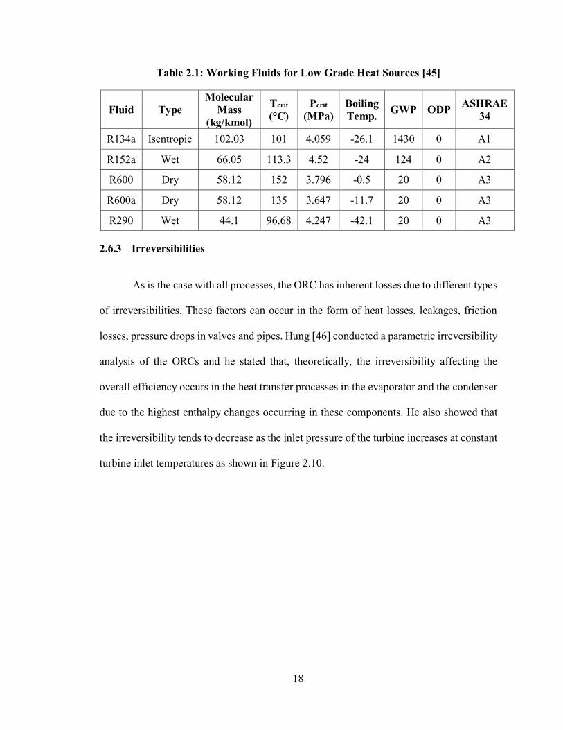
18
Table 2.1: Working Fluids for Low Grade Heat Sources [45]
Fluid Type Molecular
Mass (kg/kmol)
Tcrit (°C)
Pcrit (MPa)
Boiling Temp. GWP ODP ASHRAE
34
R134a Isentropic 102.03 101 4.059 -26.1 1430 0 A1
R152a Wet 66.05 113.3 4.52 -24 124 0 A2
R600 Dry 58.12 152 3.796 -0.5 20 0 A3
R600a Dry 58.12 135 3.647 -11.7 20 0 A3
R290 Wet 44.1 96.68 4.247 -42.1 20 0 A3
2.6.3 Irreversibilities
As is the case with all processes, the ORC has inherent losses due to different types
of irreversibilities. These factors can occur in the form of heat losses, leakages, friction
losses, pressure drops in valves and pipes. Hung [46] conducted a parametric irreversibility
analysis of the ORCs and he stated that, theoretically, the irreversibility affecting the
overall efficiency occurs in the heat transfer processes in the evaporator and the condenser
due to the highest enthalpy changes occurring in these components. He also showed that
the irreversibility tends to decrease as the inlet pressure of the turbine increases at constant
turbine inlet temperatures as shown in Figure 2.10.

19
Figure 2.10: Irreversibility-Turbine Inlet Pressure Relation for Different Working Fluids at Constant Inlet Temperature [46]
The largest portion of irreversibility in a cycle that occurs in evaporation and
condensation processes as mentioned are caused by the temperature profile differences
between the working fluid and the heat sources. Larjola [34] emphasizes that for moderate
temperature heat recovery systems, organic working fluids show higher performance and
power output compared to water-steam Rankine cycle due to the small amount of energy
needed for vaporization and better temperature profile matching with low grade heat
sources.
2.6.4 Cycle Improvements
There are certain ways to improve the performance of a cycle. However, most of
the variations cannot be easily implemented to a cycle after the configuration is complete.
The highest efficiency a thermodynamic cycle can achieve is limited by the temperatures
20
of the reservoirs as aforementioned. These temperature values define the maximum heat
transfer that can occur in a particular system.
Increasing the heat source temperature or decreasing the rejection sink temperature
would increase the overall efficiency. However, it is usually not possible to modify the
temperature of the heat rejection sink and the heat source when it comes to low temperature
energy recovery. Therefore, in order to enhance the overall performance of ORCs the
attention should be focused on the compatibility between the working fluid and the
expander, the addition of a regenerator, and mechanical and thermal efficiencies of the
components. The heat transfer efficiency in the evaporator and the expander efficiency are
considered as the main factors for efficiencies of low temperature energy recovery systems.
2.6.5 Applications
There is no standardized classification of heat sources based on their temperature
range but, different classifications are taken into considerations by many studies in the
literature. As aforementioned, Imran et. al [7] consider temperatures below than 230 °C as
low temperature heat sources. Peterson et. al [47] consider low-grade heat sources for
temperature below than 150 °C, moderate-grade for a range of 150-400 °C and high-
temperature for temperatures higher than 400 °C. Saleh et. al [42] mentioned that the low
temperature was approximately 100 °C and medium temperature was approximately 350
°C. According to U.S. Department of Energy [48], the heat sources are categorized as low-
quality for a temperature range of 0-232 °C, medium-quality for a range of 232-650 °C and
high-quality for temperatures above 650 °C.
The heat sources most commonly used in ORC applications can be divided into three main
categories as stated by Quoilin [16]:
21
Waste heat: As mentioned by Larjola [34], the ORCs are considered as the most useful
cycles for waste heat recovery systems since they can use organic fluids which provide
the best performance and the highest power output in low-grade energy recovery
compared to the traditional cycles. Hung et al. [33] indicated that 50% or more of the
overall heat generated in industry has been released to the atmosphere in the form of
low-grade energy, which also causes environmental concerns due to thermal pollution.
Waste heat recovery using ORC can also be applied to the Combined Heat and Power
(CHP) plants, cement production plants, biomass plants, exhaust gasses of vehicles,
and the condenser of power cycles.
Solar power: solar power is another heat source that can be used in ORCs since the
temperatures reached by solar panels are relatively low. Manolakos et al. [49]
conducted an experimental study on the performance analysis of a low-temperature
solar ORC (SORC) using HFC-134a as the working fluid for reverse osmosis (RO)
desalination. They obtained a maximum overall system efficiency of 4% and
approximately 2.05 kW of maximum power generation, which they believe is sufficient
to drive the RO unit.
Geothermal plants: the temperature of geothermal heat sources vary from 50 to 350 °C
and the source can be steam, mixture of steam and liquid, or only liquid water.
Hettiarachchi [38] et al. considered geothermal sources as low-temperature for a range
of 70-100 °C and they showed that the ORC efficiency using a geothermal heat source
is highly dependent on the working fluid selection and the geothermal water
temperature.
22
2.7 Comparison of Low Temperature Energy Recovery Methods
The methods mentioned above have their own advantages and disadvantages over
each other depending on a variety of working conditions such as pressure, temperature,
working fluid, etc. The transcritical CO2 and Kalina cycles are, theoretically, promising
thermodynamic cycles with high performance. However, they have not been widely proven
in the literature and, therefore, are not common in a wide range of applications. Due to
their high operating pressure conditions, these two cycles also require thicker materials
which may significantly increase the capital costs of the systems. The high toxicity of
ammonia limits the material selection in the Kalina cycle. The Stirling engine and TEG
also promise high thermodynamic performance. The main drawback of the Stirling engine
is the required operation at very high temperatures and pressures. The ORC has a minimal
number of components and is a well-developed technology with a long history of research.
It allows the use of a number of working fluids which can operate well with a variety of
heat sources. The ORC can also have high performance under a wide range of temperature
and pressure working conditions.
2.8 Expansion Machines
The expander is a key part of the ORC that has an impact on the overall performance
and efficiency of the system. There are many types of expansion machines, each of which
can work well under different system parameters and working fluids. The selection of the
most suitable expander plays a key role in achieving the optimum thermal efficiency.
Expansion machines, in general, can be divided into two main categories by their
designs and working principles. These categories are dynamic machines, such as
23
turbomachinery, and positive displacement machines, also called volumetric expanders
[15]. Positive displacement expanders include scroll, screw, rotary vane, gerotor,
reciprocating piston, rotary (rolling) piston and free-piston linear expanders. The
parameters that should be considered when selecting an expander are high isentropic
efficiency, pressure ratio, power output, rotational speed, dynamic balance, complexity,
lubrication requirements, reliability, and cost as indicated by Harada [15].
2.8.1 Turbomachinery
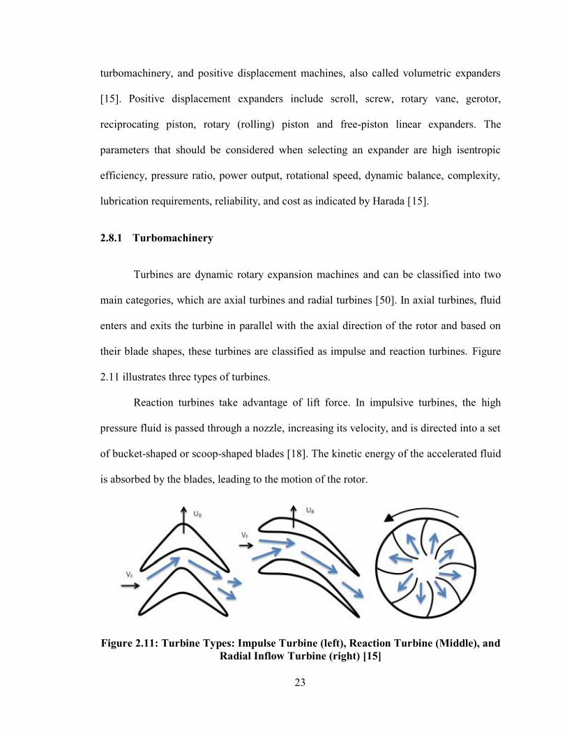
Turbines are dynamic rotary expansion machines and can be classified into two
main categories, which are axial turbines and radial turbines [50]. In axial turbines, fluid
enters and exits the turbine in parallel with the axial direction of the rotor and based on
their blade shapes, these turbines are classified as impulse and reaction turbines. Figure
2.11 illustrates three types of turbines.
Reaction turbines take advantage of lift force. In impulsive turbines, the high
pressure fluid is passed through a nozzle, increasing its velocity, and is directed into a set
of bucket-shaped or scoop-shaped blades [18]. The kinetic energy of the accelerated fluid
is absorbed by the blades, leading to the motion of the rotor.
Figure 2.11: Turbine Types: Impulse Turbine (left), Reaction Turbine (Middle), and Radial Inflow Turbine (right) [15]

24
In radial inflow turbines, the fluid enters the turbine in the axial alignment of the
center of the turbine shaft and leaves at 90° angle to the turbine shaft. Based on the direction
of flow, there are two different configurations of these turbines, centripetal (towards the
center) and centrifugal (away from the center), as shown in Figure 2.12.
Figure 2.12: Centripetal (left) and Centrifugal (right) Turbines [50]
To evaluate the performance of turbomachinery, there are several parameters that
need to be compatible with each other. However, one of the parameters that plays a key
role in the efficiency of turbomachinery is the tip speed, 𝑣, of the machine. Pressure ratio,
which is the ratio of the pressure drop per stage, determines the number of stages of the
turbomachinery and is also dependent on the tip speed [18]. There are two major tip speed-
dependent losses in displacement machines, the leakage and throttling losses. As the tip
speed increases, the leakage losses are reduced, but the throttling losses will increase [51].
The term of optimum tip speed is then defined and can be determined for any
turbomachinery. The optimum tip speed is fairly independent from the machine size, as
indicated by Persson and Sohlenius [51], and is related to the shaft speed, 𝑛, with the
following fundamental relation:
𝑛 = (𝑣 ∗ 60) (𝜋 ∗ 𝐷)⁄

25
where 𝐷 is the diameter of the expander. From this relation, it can be shown that the
expander will have to rotate at much higher rotational speeds as the diameter decreases in
order to operate at the optimum tip speed and maintain good performance. This fact makes
it impractical to use a small turbine in applications.
Depending on the design and operating conditions of the turbomachinery, the
primary source of loss can differ. Due to the interaction of the fluid with the surfaces of the
blades, the housings, and the rotor hub, fluid friction occurs in the boundary layer. The
boundary-layer losses can be considered as the inevitable and most important loss source
of up to 30 percent of the machine output [18]. Another source of loss is due to the blade
tip leakage. A portion of the fluid flow tends to leak from the clearance between the blade
tips and the housings resulting in a loss due to the decrease in the mass flow and the change
in the flow pattern in the blade tips. This clearance is machine-sized and kept to a minimum
regardless of the size of blades. For large blades, the tip leakage losses amount to 1-2
percent. However, relatively the same loss may account for 10-15 percent in small scale
turbines [18]. Other sources that contribute to loss in efficiency include seal leakage (1%),
eddy losses (1-2%), moisture churning (1% per 1% of moisture), and bearing losses (<1%)
[18].
Yamamoto et al. [52] performed a numerical and experimental study on the
efficiency of an ORC using a micro-turbine. The turbine was a radial type, made of
aluminum, with 18 blades, 30 mm in diameter and 4.5 mm thick. The maximum isentropic
efficiency that the turbine achieved was shown as 46%, however, any deviation from the
designed conditions caused a rapid decrease in the turbine efficiency. The maximum cycle
efficiency was obtained as 1.25% by using HCFC-123 as the working fluid.
26
Yagoup et al. [53] conducted an experimental study on a micro-CHP ORC utilizing
solar energy as the heat source. The total capacity of the solar source was 25 kW and the
maximum turbine capacity was 1.5 kW. The turbine rotated at 60,000 RPM and they
achieved 85% turbine isentropic efficiency using HFE-301. The maximum electrical and
overall cycle efficiencies were obtained as 7.6% and 17%, respectively.
Kang [54] designed a radial turbine with a pressure ratio of 4.1 and an ORC. He
also conducted experiments in different evaporator temperatures to analyze the efficiencies
and the operational characteristics of the system. He showed that the efficiencies of both
the turbine and overall cycle increased as the evaporator temperature increased. Maximum
average cycle and turbine efficiencies and power output were achieved as 5.2%, 78.7%,
and 32.7 kW, respectively, using a low temperature heat source and R245fa as the working
fluid.
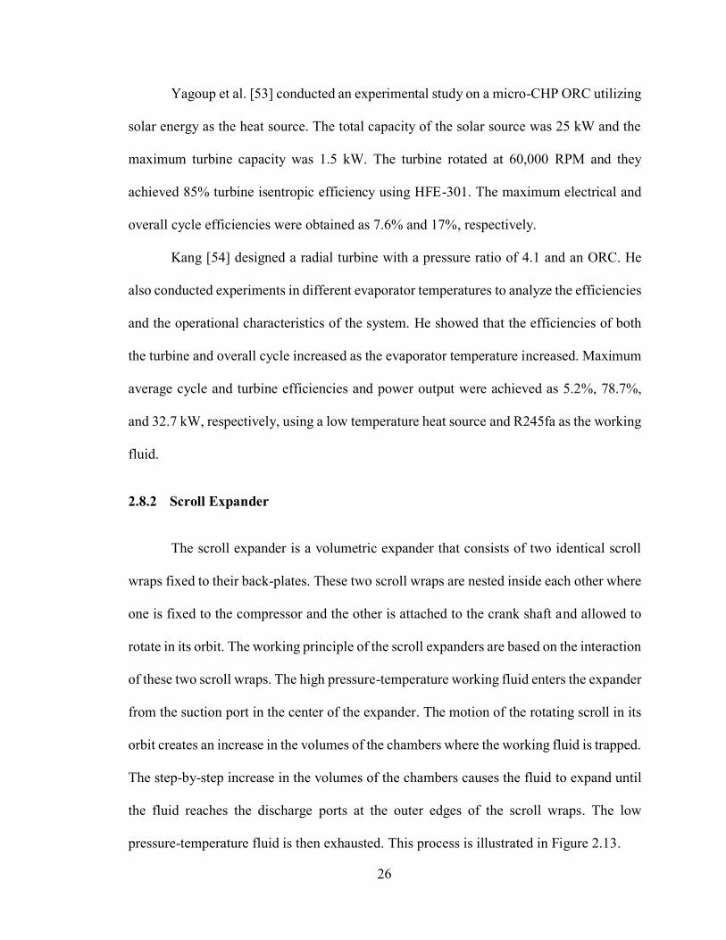
2.8.2 Scroll Expander
The scroll expander is a volumetric expander that consists of two identical scroll
wraps fixed to their back-plates. These two scroll wraps are nested inside each other where
one is fixed to the compressor and the other is attached to the crank shaft and allowed to
rotate in its orbit. The working principle of the scroll expanders are based on the interaction
of these two scroll wraps. The high pressure-temperature working fluid enters the expander
from the suction port in the center of the expander. The motion of the rotating scroll in its
orbit creates an increase in the volumes of the chambers where the working fluid is trapped.
The step-by-step increase in the volumes of the chambers causes the fluid to expand until
the fluid reaches the discharge ports at the outer edges of the scroll wraps. The low
pressure-temperature fluid is then exhausted. This process is illustrated in Figure 2.13.
27
Figure 2.13: Working Process of a Scroll Expander [55]
There are two types of scroll expanders; compliant type and kinematically
constrained type. The constrained type of expanders is usually made of three cranks
separated from each other by an angle of 120°. The orbiting scroll is constrained axially,
radially, or both. Thus, two scroll wraps do not interact with each other during the operation
and there is a small clearance gap between them. Therefore, they do not require lubrication,
but sealing becomes the paramount factor on their performance. The gaps have to be
minimized during manufacturing to reduce leakage losses. Constrained expanders are more
effective when used at higher rotation speed because the time that the working fluid has to
escape from the chambers is reduced at higher speeds. In the compliant type of expanders,
however, an orbiting scroll is present and they use the centrifugal effect during operation.
The scrolls are always in contact. Therefore, lubrication is needed to prevent overheating
of the scrolls and to reduce frictional losses. Low friction materials are used in the
28
compliant scroll types for sealing and they have better sealing compared to the constrained
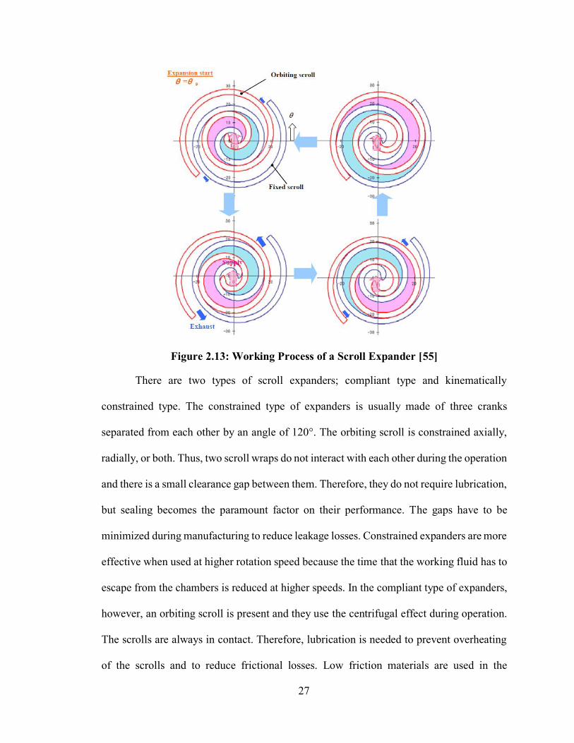
types [15]. In scroll expanders, there are two leakage passages; radial leakage and flank
leakage, as illustrated in Figure 2.14 [56].
Figure 2.14: Flank and Radial Leakages [56]
Scroll expanders are commonly used in small power output applications with a
wide range of isentropic efficiencies between 50-89% as indicated by Kinnaly and
Nuszkowski [17]. An experimental study by Lemort et al. [57] was carried out on a
prototype of an open-drive oil-free scroll expander using HCFC-123 in an ORC. The
results showed that the tested prototype reached a maximum isentropic efficiency of 68%.
Another experimental study by Mathias et al. [58] was conducted on a scroll expander used
in an ORC. They obtained an isentropic efficiency of 83% for the scroll expander with an
electric production of 2.96 kW. They also concluded that the scroll expanders were good
candidates to be used in power production from low-grade energy.
29
2.8.3 Screw Expander
The screw expander, a type of volumetric expander, was developed to utilize the
energy in geothermally hot water in the 1970s [59]. They can have expansion ratios up to
3:1 [50]. Two different screw expander designs exist: the twin screw and single screw
designs.
The twin screw expander consists of three parts; a casing and a meshing pair of two
helical screw rotors that are called female and male rotors. The male rotor is known as the
rotor with a larger diameter, whereas the female rotor has smaller thickness. Helical screws
of both rotors mesh and rotate in opposite directions. The fluid flows through the intake
port. As the pressurized hot fluid drives the rotors (mechanical energy extraction), the
volumes of v-shaped expansion chambers increase, thereby leading to the expansion of the
fluid. Then, the depressurized warmer fluid is exhausted when the expansion chamber
reaches the discharge port. Figure 2.15 illustrates the operation of a twin screw expander
from intake to discharge.

30
Figure 2.15: Working Processes of a Twin Screw Expander [17]
The single screw expander, on the other hand, has a single helical screw rotor (main
rotor) with, additionally, two gate rotors located symmetrically on each side of the main
rotor. The only difference in the working process of the single screw expander from the
twin screw expander is that the fluid is trapped with the gate rotors instead of using two
helical rotors. Figure 2.16 shows the working processes of a single screw expander.
Figure 2.16: Working Mechanism of a Single Screw Expander [60]
31
For efficient operation of the screw expanders, Smith et al. [61] suggests the
following:
Maximum flow area between the lobes and casing
Minimum leakage
Optimum choice of built-in volume ratio
Optimum choice of tip speed
The main challenge of the screw expanders is preventing the internal leakages
between the expansion chambers and between the shafts and casing while keeping the
contact surface friction minimized [50]. Two methods for screw expanders have been
developed to overcome this situation: oil-free and oil injection designs. In oil injection
designs, the working fluid is mixed with oil in order to seal the clearances, lubricate the
rotor motion, and prevent overheating of the machine. No internal sealing is required in
this type of design. It has a simpler mechanical design, is inexpensive to manufacture and
highly efficient [62]. In the oil-free machines, oil is separated from the working fluid and
lubrication of the bearings is done externally. Internal seals are required to avoid lubricant
entering the rotor lobes. Timing gears are used to prevent contact between rotors. These
additional parts require a more sophisticated design and manufacturing costs than needed
for the oil injection design [62,63].
Screw expander applications include ORC, SORC, geothermal, refrigeration
cycles, and trilateral flash cycle for low-grade heat sources [17]. Long term developments
and investigations have been carried out by Smith et al. [61,62,64]. They emphasized that
the screw expanders are the expanders most suitable with two-phase working conditions
and they achieved a peak isentropic efficiency of 76% [62].

32
2.8.4 Rotary Vane Expander
Another type of volumetric expander is the rotary vane expander and it has a simple
mechanical design consisting of a housing and rotor with sliding vanes. The design and
operation of this expander are illustrated in Figure 2.17. Operation of this expander starts
with the pressurized fluid entering the inlet (1). The sliding vanes that are located inside
the rotor are pushed outward by the centrifugal effect driving the rotor and extracting the
mechanical energy. As the vanes rotate, the volume in the expansion chamber increases (2-
3). Thus, the fluid expands and, at the end, is discharged from the outlet (4).
Figure 2.17: Design and Working Processes of a Rotary Vane Expander [15]
Rotary vane expanders have several advantages over other types such as low
manufacturing cost due to their simple designs and minimal mechanical parts, capability
of handling high pressure, high tolerances to operate under wet expansion conditions with
little or no erosion [65,66]. They also have relatively high volumetric expansion ratios
ranging up to 10 and cause low noise and vibration during operation [66]. Lubrication is
33
required in order to enhance sealing, prevent overheating, reduce friction losses and
minimize wear during operation [67]. It is also mentioned by Badr et al. [66] that the main
power losses occur due to the pressure drop at the inlet accounting for 65% of the total loss,
whereas leakage losses account for 20%.
In a study conducted by Yang et al. [68], a rotary vane expander prototype was
tested in the transcritical CO2 refrigeration cycle with a suction pressure range from 7.5 to
9.0 MPa and a suction temperature range from 32.4 to 44.3 °C. The optimal isentropic
efficiency of 23% was obtained at 800 RPM. To clarify that the efficiency decreased at
higher speeds, the authors concluded that the frictional losses increased more rapidly than
the reduction in the leakage losses via better sealing at higher speeds. Kinnaly and
Nuszkowski reported that the maximum output power output of a rotary vane expander in
the literature was found to be less than 2 kW with an isentropic efficiency range between
23-73% [17].
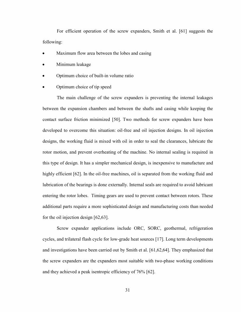
2.8.5 Gerotor Expander
The gerotor is a volumetric rotary expansion machine that consists of an inner rotor
and outer stator located eccentrically on the same shaft. In the design, the rotor has one less
tooth than the stator and the expansion chamber volumes constantly change as the shaft is
rotated by the high pressure fluid. The expansion process of the gerotor is shown in Figure
2.18. During half of each shaft rotation, the expansion chamber volumes increase (1-5) and
they start decreasing through the second half of shaft rotation (6-10). Via inlet port, the
fluid enters the expansion chamber at the minimum volume and expands as the volume
increase. The depressurized fluid is forced out when it reaches the exit port. While the
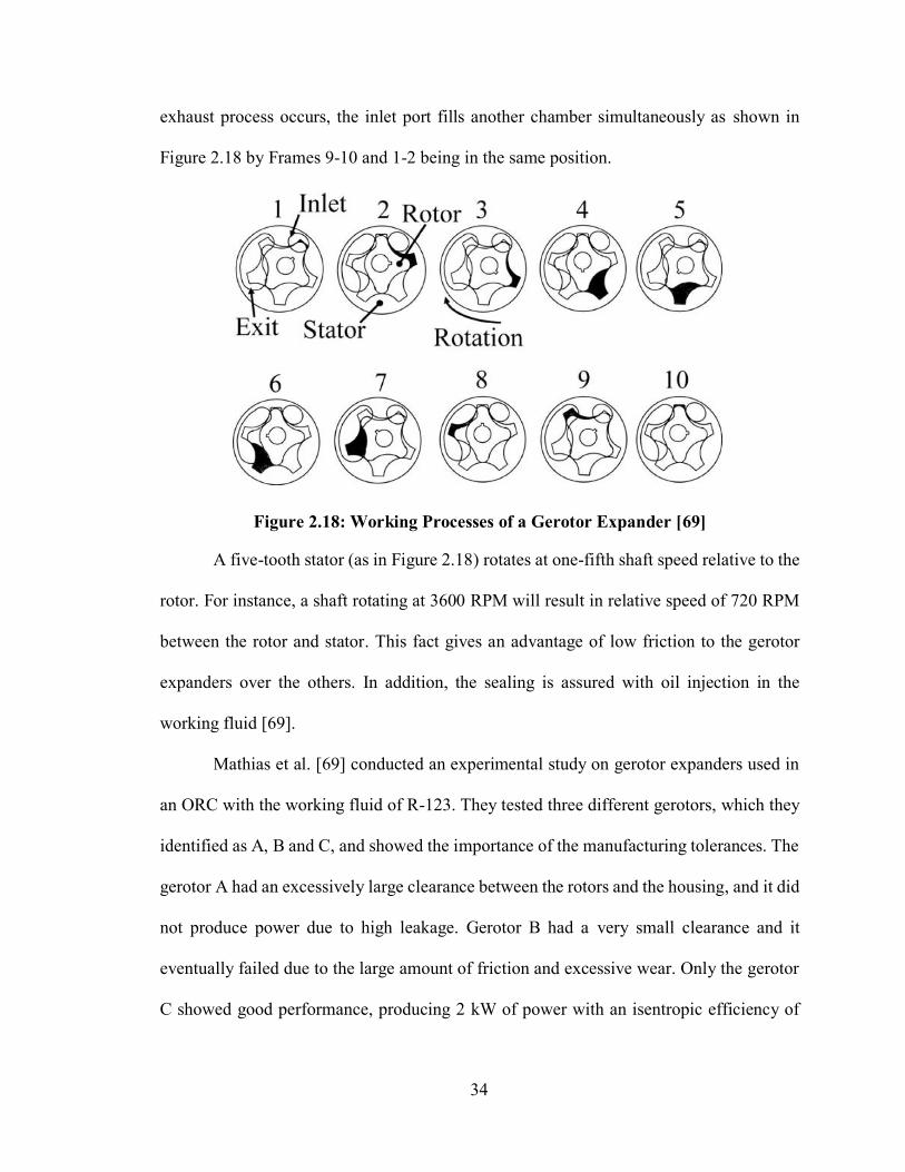
34
exhaust process occurs, the inlet port fills another chamber simultaneously as shown in
Figure 2.18 by Frames 9-10 and 1-2 being in the same position.
Figure 2.18: Working Processes of a Gerotor Expander [69]
A five-tooth stator (as in Figure 2.18) rotates at one-fifth shaft speed relative to the
rotor. For instance, a shaft rotating at 3600 RPM will result in relative speed of 720 RPM
between the rotor and stator. This fact gives an advantage of low friction to the gerotor
expanders over the others. In addition, the sealing is assured with oil injection in the
working fluid [69].
Mathias et al. [69] conducted an experimental study on gerotor expanders used in
an ORC with the working fluid of R-123. They tested three different gerotors, which they
identified as A, B and C, and showed the importance of the manufacturing tolerances. The
gerotor A had an excessively large clearance between the rotors and the housing, and it did
not produce power due to high leakage. Gerotor B had a very small clearance and it
eventually failed due to the large amount of friction and excessive wear. Only the gerotor
C showed good performance, producing 2 kW of power with an isentropic efficiency of
35
85%. Thus, they showed that the performance of the gerotor highly relied on the
manufacturing tolerances.
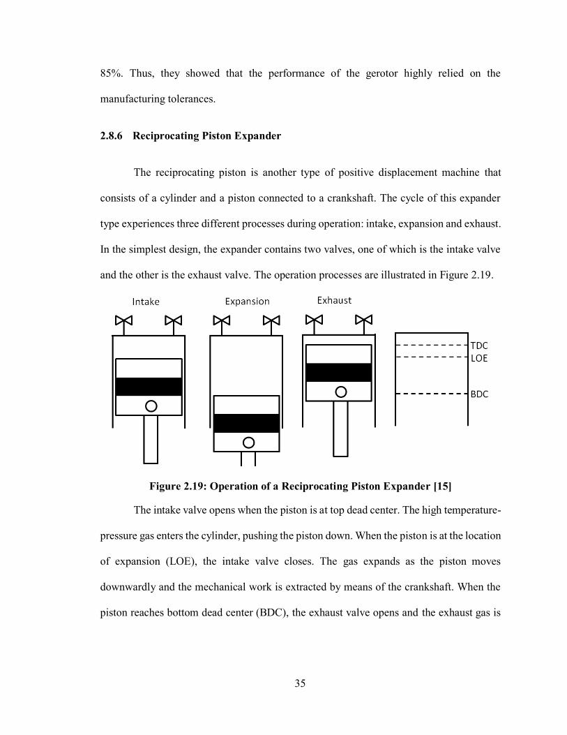
2.8.6 Reciprocating Piston Expander
The reciprocating piston is another type of positive displacement machine that
consists of a cylinder and a piston connected to a crankshaft. The cycle of this expander
type experiences three different processes during operation: intake, expansion and exhaust.
In the simplest design, the expander contains two valves, one of which is the intake valve
and the other is the exhaust valve. The operation processes are illustrated in Figure 2.19.
Figure 2.19: Operation of a Reciprocating Piston Expander [15]
The intake valve opens when the piston is at top dead center. The high temperature-
pressure gas enters the cylinder, pushing the piston down. When the piston is at the location
of expansion (LOE), the intake valve closes. The gas expands as the piston moves
downwardly and the mechanical work is extracted by means of the crankshaft. When the
piston reaches bottom dead center (BDC), the exhaust valve opens and the exhaust gas is

36
expelled from the system by the piston moving upwardly. When the piston reaches TDC,
the intake valve opens and, thus, one cycle is completed.
The reciprocating piston expander is very robust, which is an advantage over the
other expanders. However, for efficient operation, they require structure balancing to
prevent excessive vibrations and precise timing of the intake and exhaust valves with the
piston motion [50]. Sealing is assured by the use of piston rings. The primary contribution
to the performance losses is the friction due to the large contact surfaces between the rings
and the cylinder wall. Therefore, a lubricant such as oil is also required to reduce the
friction losses and to avoid excessive wear.
Zhang et al. [70] developed a double acting free piston expander to replace the
throttling valve for work recovery in the transcritical CO2 cycle. They achieved an
isentropic expander efficiency of 62% and they also stated that utilizing a slider-based
inlet/outlet control scheme led to proper operation of the expander and an increase in the
efficiency. In another study by Baek et al. [71], a piston expander replaced the expansion
valve in a transcritical CO2 refrigeration cycle with a goal to increase the coefficient of
performance (COP) of the system. The expander was a modified four-cycle, two-piston
gasoline engine with a displacement volume of 2×13.26 cm3.The expander achieved an
isentropic efficiency of approximately 11%, enhancing the system performance (COP) by
up to 10.5%.
Glavatskaya et al. [72] modelled a semi-empirical reciprocating expander for
exhaust heat recovery in an automobile application. The expander achieved a maximum
isentropic efficiency of 70%. They also observed and stated that the isentropic efficiency
37
of the expander increased with the rotary speed, but decreased as the pressure ratio on the
expander increased.
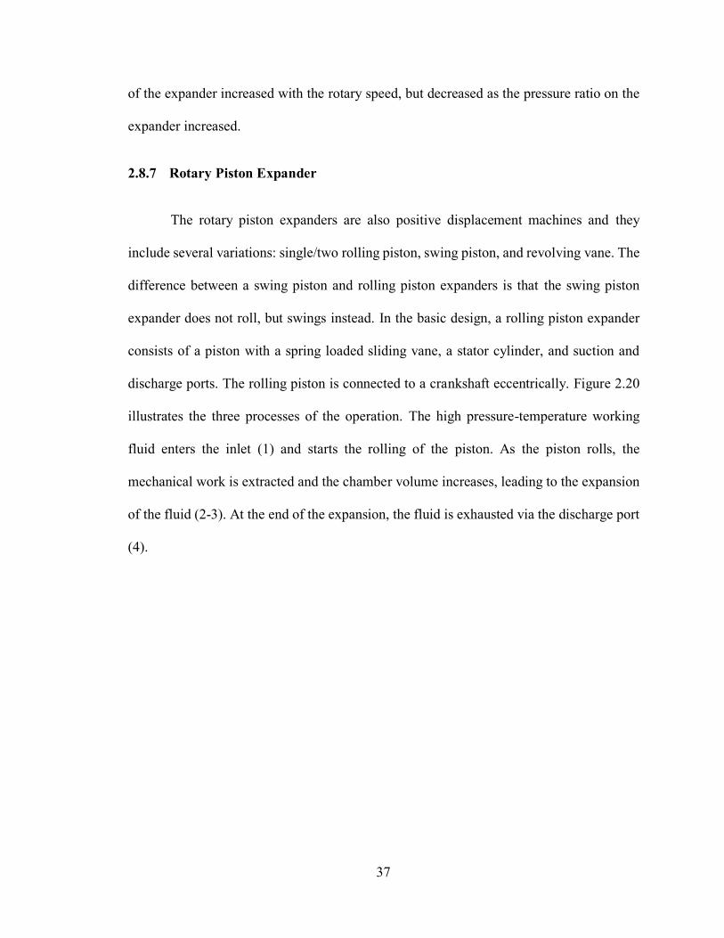
2.8.7 Rotary Piston Expander
The rotary piston expanders are also positive displacement machines and they
include several variations: single/two rolling piston, swing piston, and revolving vane. The
difference between a swing piston and rolling piston expanders is that the swing piston
expander does not roll, but swings instead. In the basic design, a rolling piston expander
consists of a piston with a spring loaded sliding vane, a stator cylinder, and suction and
discharge ports. The rolling piston is connected to a crankshaft eccentrically. Figure 2.20
illustrates the three processes of the operation. The high pressure-temperature working
fluid enters the inlet (1) and starts the rolling of the piston. As the piston rolls, the
mechanical work is extracted and the chamber volume increases, leading to the expansion
of the fluid (2-3). At the end of the expansion, the fluid is exhausted via the discharge port
(4).
38
Figure 2.20: Intake, Expansion, and Discharge Processes of a Rolling Piston Expander [15]
These types of expanders are able to handle very high pressures, and also have
simple designs with few parts. The main sources of performance losses are friction and
internal leakages. Lubrication is necessary to minimize friction and wear, and to assure
sealing. The primary internal leakage occurs at the interaction surfaces of the piston and
the cylinder wall due to the high pressure differential between the neighboring volumes
[73].
Wang et al. [74] conducted an experimental study on a rolling piston expander used
in a solar Rankine cycle with R-245fa as the working fluid. The tested expander achieved
an average isentropic efficiency of 45.2% at 800-900 RPM, producing an average power
output of 1.73 kW. Haiqing et al. [73] developed a swing piston expander prototype to
replace the throttling valve in a CO2 transcritical cycle. They obtained an isentropic
efficiency range generally between 28% and 44% for the expander and mentioned that the
39
friction and leakage losses must be evaluated carefully in the design of this type of
expander. Jiang et al. [75] designed a two-rolling piston expander and tested the expander
in a transcritical CO2 cycle. In a range of rotation speed from 850 to 1000 RPM, the
expander achieved an isentropic efficiency of 28-33%. In another study carried out by Hu
et al. [76], a two-rolling piston expander prototype was developed and tested in a CO2
transcritical heat pump system. The expander achieved a maximum efficiency of 77% at
the rotation speed of 867 RPM.
2.8.8 Free-Piston Linear Expander
The free-piston linear expander (FPLE) is a positive displacement machine that
converts thermal energy directly into electrical energy. It has been a subject of research in
recent years and a few design alternatives are proposed in the literature [78-83]. In its
traditional design, the FPLE consist of a piston that is free to move within a bore from TDC
to BDC without a mechanical linkage, unlike the typical design of the reciprocating piston
expander. One of the compact designs is considered to be the free-piston with double-
piston structure [79] or, in another words, a piston with two chambers structure [6,77,78].
It consists of a piston with two chambers and a cylinder with four ports, two of which are
intake ports and the others are exhaust ports. The cylinder housing has an electric coil. The
piston has two chambers connected to each other with a rod, to which permanent magnets
are coupled. In each chamber, there are intake and exhaust ports. Figure 2.21 illustrates an
example of a piston with two chambers structure of a FPLE. It should be noted that the
FPLE design in Figure 2.21 does not use control valves to control the opening of the intake
and exhaust ports [6,77,78], unlike other designs [79].

40
The FPLE, designed by Bonar [6], was designed in such a way that the port of the
first chamber of the piston is aligned with the intake port of the cylinder while the port of
the second chamber of the piston is in exhaust position, and vice versa. The pressurized
working fluid enters the first chamber, creating high-low pressure differential between the
two chambers. The piston starts moving in one direction until the second chamber is
aligned with intake port of the cylinder and the first chamber is positioned in the exhaust
port of the cylinder. The depressurized fluid in the first chamber is then discharged from
the exhaust port while the pressurized fluid enters the second chamber of the piston via the
intake port of the cylinder. The pressure differential is now created in the opposite
direction, directing the piston to move in the opposite direction. When the depressurized
fluid in the second chamber reaches the exhaust port, the fluid is pushed out and the
pressurized fluid enters the first chamber of the piston through the intake port of the
cylinder, completing one cycle. As the piston reciprocates, the magnets coupled to the
connecting rod create a magnetic field in the electric coils coupled to the cylinder housing,
which is converted into electricity [6].

41
Figure 2.21: Cut-away View of a FPLE [77]
One of the major advantages of this expander is its simple and low manufacturing
cost. The expander also has only one moving part, the piston, since the intake and exhaust
ports are valveless. On the other hand, the major contributions to the performance losses
are due to the friction between the piston and the cylinder wall, heat loss from the cylinder,
and the internal leakages between the piston and the cylinder walls.
Nuszkowski et al. [78] modelled and tested a FPLE to analyze the performance of
the expander using air as the working fluid. The expander did not succeed in running for
periods over ten minutes and due to the electrical generator operating without a load, the
isentropic efficiency of the system was zero. However, they achieved a maximum
isentropic efficiency of 42% from the parametric study. Hawn et al. [77] designed and
tested a FPLE that involved several changes from the expander tested previously by
Nuszkowski et al. Air was used as the working fluid. However, the expander failed to
achieve the desired steady-state operation due to the seizing of the piston inside the cylinder
housing.
42
Wang et al. [79] conducted an experimental study of a dual-piston air-driven free-
piston linear expander coupled with a linear electric generator. In their conceptual design,
the air flow into and out of the system was managed by using intake valve and electro-
magnetic exhaust valve in each cylinder. They investigated the operational characteristics
of the FPLE, which included the piston dynamics, output voltage, operation frequency, and
system energy conversion efficiency, at a driven air pressure range between 2-3.75 bar. It
was concluded that the expander reached to higher frequency and system energy
conversion efficiencies as the driven air pressures increased. The authors also stated that
the configuration of the FPLE, compared to the conventional expansion machines, presents
significant benefits, such as compact design, low frictional loss, high efficiency, and good
operational flexibility [79].
Zhang et al. [80] developed a design of a double acting free piston expander to
recover the work in the throttling process of the transcritical CO2 cycle. A slider-based
inlet/outlet control scheme was used to ensure the proper suction, expansion, and discharge
processes during operation. The expander was experimentally validated and showed stable
operation in a wide range of pressure differences between the inlet and outlet conditions.
The optimal working frequency range was observed to be between 10 to 17 Hz and the
isentropic efficiency of 62% was achieved from the p-V diagram.
Preetham and Weiss [81] designed a small-scale free piston expander based on a
sliding-piston architecture and investigated its operation to use in the conversion of low
temperature waste heat sources into useful power output. The control variables were chosen
as piston mass, input heat rate, duration of heat input, and external load. The output
conditions and trends such as efficiency, operating frequency, and output power were

43
evaluated to identify optimal performance characteristics. It was observed that increasing
the heat inputs into the expander resulted in an increase in the power output while
decreasing the operating frequency. From the results, the expander efficiency was
concluded to be dependent on design parameters, mainly the piston mass and heat input
rate.
Champagne and Weiss [82] constructed a millimeter scale free piston expander to
use in the low temperature waste heat recovery and its operational parameters were
examined to characterize and optimize the piston motion. The optimized parameters
included piston sealing, lubrication, piston length, FPE cross sectional area, and input
pressure. The results indicated that as the viscosity of the lubricant increased, more efficient
sealing was achieved in static environments. The thinner lubricants increased sealing in
dynamic motion of the piston.
Li et al. [83] proposed to recover waste heat from vehicle engines by using a novel
free-piston expander-linear generator integrated unit. The unit consisted of two free piston
expanders and a linear generator connected to each other with piston rods and flexible
joints. The intake and exhaust processes of the expander were controlled by mechanical
control valve trains driven by servo motors, and the dynamic characteristics of the in-
cylinder flow field during the gas inlet-outlet processes were analyzed by using 3-D
numerical simulation models. The results indicated that the expander was capable of
achieving an efficiency of 66.2% and produce a maximum electrical power output of 22.7
W when the working frequency and intake pressure were 3 Hz and 0.2 MPa, respectively.

44
2.8.9 Comparison of Expanders
Each expander has advantages and disadvantages depending on several criteria
such as its operational limitations, performance, reliability, cost, and noise. Therefore,
several parameters need to be evaluated when selecting an expander. Considerations of
each type of expanders are presented in summary below.
Turbomachinery: Turbines have a good reputation for high isentropic efficiency
and reliability at large scale power generation systems. At small-scale power generation,
however, they require excessively high speeds to operate efficiently as the machine size
gets smaller. They are also not tolerant of wet expansion and have complicated designs and
high manufacturing costs. They are able to achieve isentropic efficiencies as high as 85%,
but limited number of studies exists in the literature for small scale power generation.
Scroll Expander: The scroll expanders have been extensively tested in the literature
and are commonly used in a variety of applications. The most crucial factor affecting the
performance is the leakage. They have complicated geometry and require strict
manufacturing tolerances. The scroll expanders are able to operate with wet fluid and have
shown isentropic efficiencies as high as 89% in small scale power generation systems.
Screw Expander: The screw expanders have complicated rotor geometry, but robust
design. The main challenge of this expander type is sealing which can be assured with oil
injection. They are able to handle operations at very high pressure with isentropic
efficiencies as high as 76% in small scale power generation systems.
Rotary Vane Expander: This type of expanders has a simple and robust design, and
low manufacturing cost. They are capable of handling high operational pressures and have
high tolerances of wet expansion. Friction and leakage are the major performance losses.

45
The rotary vane expanders are able to achieve isentropic efficiencies as high as 73%, but
studies on this type of expanders are in limited number in the literature.
Gerotor Expander: In gerotor expanders, both the housing and the rotor rotate and
they have complex, but robust design. It can handle high pressures and wet expansion. A
relatively low rotational velocity between the rotor and stator provides the advantage of
lower friction loss. It is recorded that the gerotor expander was able to achieve an isentropic
efficiency of 85%. However, they have not been extensively researched in the literature.
Reciprocating Piston Expander: This expander has a robust design, but is subjected
to high frictional losses due to the large contact surfaces. It requires precise valve timing,
and vibrations may occur if the structural balance is not assured. They are able to achieve
isentropic efficiencies up to 70%, but no literature was found on their performance in an
ORC.
Rotary Piston Expander: The rotary piston expander has a simple and robust design,
and low manufacturing cost with few parts. It is able to handle high pressure. The main
challenge of this expander is to reduce friction and leakage between the piston and the
cylinder wall. It has been documented to have an isentropic efficiency of 77%. However,
there are a limited number of studies on their performance in an ORC in the literature.
Free-Piston Linear Expander: The configuration of FPLE involves several
advantages over conventional expansion machines, such as compact and simple design,
low manufacturing cost, good operational flexibility, and high efficiency. Friction and
leakage are assumed to be prominent factors on its performance. Another contribution to
performance losses is a possible heat loss which can be minimized with proper insulation
techniques. In addition, structural balancing is required to prevent excessive vibrations.
46
Research and development studies on FPLE exist in limited number in the literature. Only
one study presents the electrical performance by the free-piston linear expander [79].
Many studies have been observed on conventional expansion machines in the
literature. Although the FPLE has a simple design and low manufacturing cost, a limited
number of experimental studies on this expander exists in the literature. For this reason,
the objective of this study was to develop a FPLE to investigate its performance for use in
low temperature energy recovery systems.
47
3 Experimental Setup and Analysis
The objective of this work was to investigate the performance of the FPLE and to
analyze its viability for low temperature heat recovery systems. Heat sources such as waste
energy, solar power, and geothermal energy can be utilized to drive the selected expander.
However, as aforementioned, a limited number of experimental studies of the FPLE were
found in the literature. For this reason, primary attention was focused on the initial
operation of the FPLE. For this study, the testing was performed at the University of North
Florida’s College of Computing, Engineering & Construction’s Mechanical Engineering
Energy Efficiency Laboratory by using the air as the working fluid provided by means of
a compressor. In order to analyze the performance of the FPLE and to compare it with other
expander types in the literature, a test bench was developed with measurement devices such
as pressure and temperature sensors, LabJack U12, and flow rate meter. The schematic of
the testing configuration is shown in Figure 3.1. Below is a brief explanation of the
expander design, equipment, measurement devices, and the method of thermodynamic
analysis.
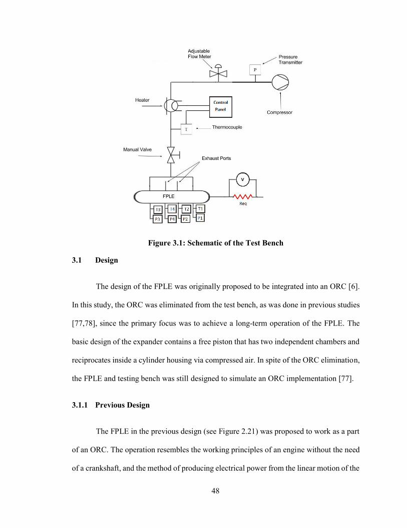
48
Figure 3.1: Schematic of the Test Bench
3.1 Design
The design of the FPLE was originally proposed to be integrated into an ORC [6].
In this study, the ORC was eliminated from the test bench, as was done in previous studies
[77,78], since the primary focus was to achieve a long-term operation of the FPLE. The
basic design of the expander contains a free piston that has two independent chambers and
reciprocates inside a cylinder housing via compressed air. In spite of the ORC elimination,
the FPLE and testing bench was still designed to simulate an ORC implementation [77].
3.1.1 Previous Design
The FPLE in the previous design (see Figure 2.21) was proposed to work as a part
of an ORC. The operation resembles the working principles of an engine without the need
of a crankshaft, and the method of producing electrical power from the linear motion of the

49
piston is performed by means of magnets coupled to the piston and a coil lined to the
cylinder. During its operation, the parameters in each chamber change simultaneously and
electrical power is produced as one chamber expands while the other chamber compresses.
This process is briefly described in Table 3.1 below.
Table 3.1: Chamber-to-Chamber Working Processes
Process Left Chamber Right Chamber
1 → 2 Air Discharge Air Suction
2 → 3 (Power Extraction) Compression Expansion
3 → 4 Air Suction Air Discharge
4 → 1 (Power Extraction) Expansion Compression
The working fluid in an ORC is an organic fluid that is pressurized and then
vaporized before entering the expander. However, air was chosen as the working fluid in
the previous study [77]. To simulate the expander as a part of an ORC, the organic fluid
was modeled. The pressures and the fluid flow rate determined from the parametric model
were kept consistent with the use of air. Therefore, the operation of the FPLE was simulated
as it would operate in an ORC with an organic fluid. The expander was proposed to
generate 60 W and to show an isentropic efficiency of 60% with the following assumptions
[77]:
Air is considered as an ideal gas
Heat loss is negligible
The piston is perfectly sealed

50
The magnet weight in the piston void is the same as if the void is filled with
aluminum
3.1.2 Modifications
Several issues in the previous design were addressed to enhance the performance
of the FPLE. Amongst those, the major attention was paid to frictional losses and sealing
issues. The leakage was foreseen to occur due to the gap between the piston and the
cylinder wall and also in the flange connections of the cylinder. These gaps would cause
the leakage of the inlet fluid to both chambers while one of the chambers needs to exhaust
the expanded fluid. Leakage due to the gaps would also be caused by air moving from one
chamber to another of the piston since the two zones were not sealed in the design. Besides
the fact that the leakage would cause a loss in the mass flow rate, thereby in the
performance, the primary issue would be the pressure differences between the zones not
being created as required and hindering the movement of the piston inside the cylinder.
The gaps in the flange connections of the cylinder, on the other hand, will cause the leaking
of the air from inside of the cylinder to the environment, adversely affecting the
performance of the expander.
Three silicone rubber O-rings on each chamber of the piston (six in total) were used
to manage the fluid flow as desired. These rings enhanced the sealing between the cylinder
wall and the piston, and also separated the two zones to provide sealing between the two
chambers. The reasons for choosing the silicone rubber O-rings are their resistant to high
temperatures up to 260 °C and hardness characteristics with a durometer of 70A. However,
it was known that the use of three O-rings would increase the contact surface which leads
to increased friction. For this reason, a multi-purpose synthetic grease resistant to
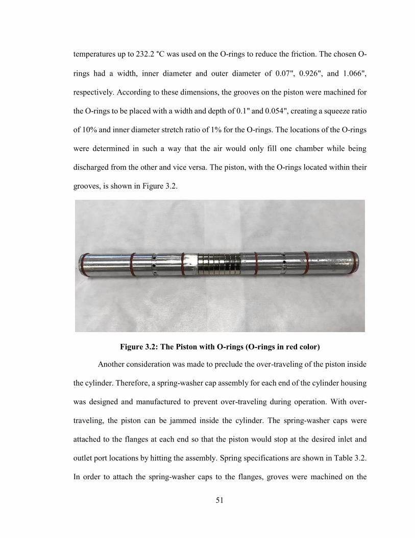
51
temperatures up to 232.2 °C was used on the O-rings to reduce the friction. The chosen O-
rings had a width, inner diameter and outer diameter of 0.07", 0.926", and 1.066",
respectively. According to these dimensions, the grooves on the piston were machined for
the O-rings to be placed with a width and depth of 0.1" and 0.054", creating a squeeze ratio
of 10% and inner diameter stretch ratio of 1% for the O-rings. The locations of the O-rings
were determined in such a way that the air would only fill one chamber while being
discharged from the other and vice versa. The piston, with the O-rings located within their
grooves, is shown in Figure 3.2.
Figure 3.2: The Piston with O-rings (O-rings in red color)
Another consideration was made to preclude the over-traveling of the piston inside
the cylinder. Therefore, a spring-washer cap assembly for each end of the cylinder housing
was designed and manufactured to prevent over-traveling during operation. With over-
traveling, the piston can be jammed inside the cylinder. The spring-washer caps were
attached to the flanges at each end so that the piston would stop at the desired inlet and
outlet port locations by hitting the assembly. Spring specifications are shown in Table 3.2.
In order to attach the spring-washer caps to the flanges, groves were machined on the
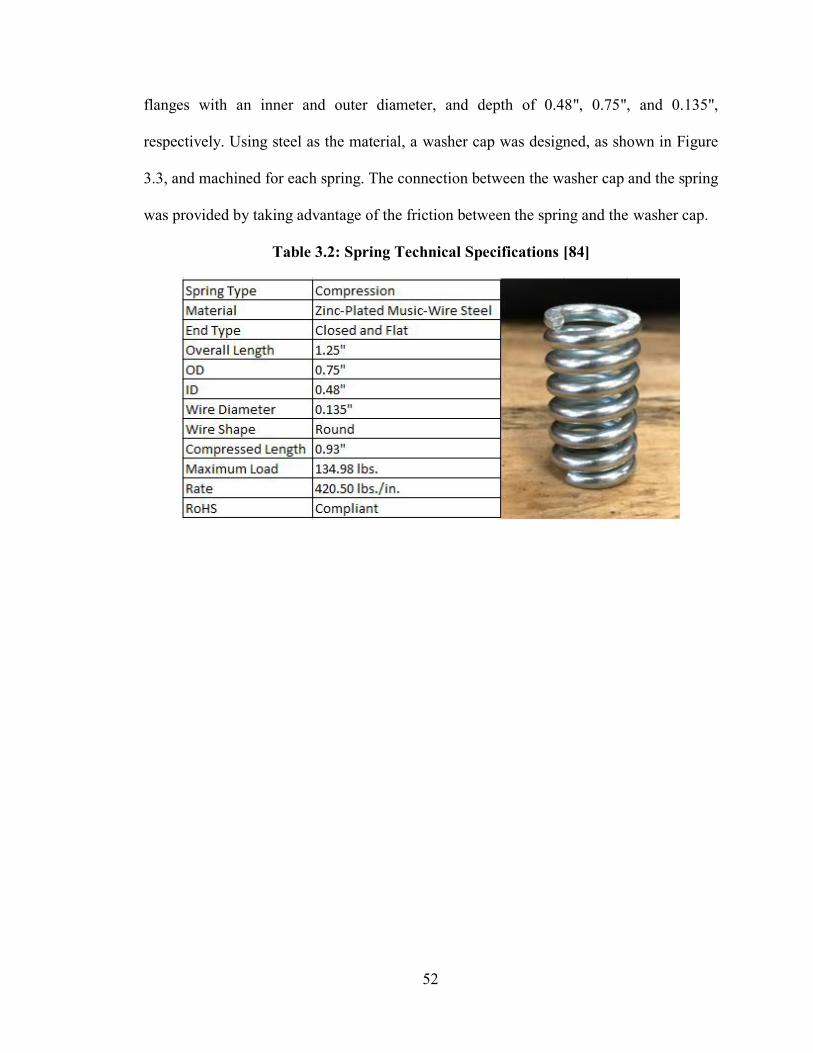
52
flanges with an inner and outer diameter, and depth of 0.48", 0.75", and 0.135",
respectively. Using steel as the material, a washer cap was designed, as shown in Figure
3.3, and machined for each spring. The connection between the washer cap and the spring
was provided by taking advantage of the friction between the spring and the washer cap.
Table 3.2: Spring Technical Specifications [84]

53
Figure 3.3: 2-D Drawing of the Washer Cap with Dimensions
The sealing at the flange connections of the cylinder was provided via the use of
silicone rubber O-rings with the width, inner diameter, and outer diameter of 0.210",
1.475", and 1.895", respectively. According to the O-ring’s dimensions, an additional
groove on each flange was machined with an inner and outer diameter, and depth of 1.505",
1.925", and 0.146", respectively, creating a squeeze ratio of 30% and inner diameter stretch
ratio of 2% for the O-Rings. The Figure 3.4 presents one of the flanges with O-ring and
spring-washer cap assembly located in their grooves.

54
Figure 3.4: The Flange of the Cylinder with O-ring and the Spring-Washer Cap Assembly
Due to inadequate heating and restriction in the flow rate, the heater used in the
previous design was replaced with AHP-7561 in-line air heater. The AHP-7561 in-line air
heater was capable of providing 750 W with a maximum volumetric flow rate of 20 cfm
and was used to heat the air before entering to the FPLE. Table 3.3 presents the technical
specification of the AHP-7561.

55
Table 3.3: Heater Technical Specifications [85]
To reduce the heat being released to the environment during the operation of the
FPLE, the cylinder vessel and the inlet air pipeline were insulated with a fiberglass
insulation material. The technical specifications of the insulation material are shown in the
Table 3.4 below.
Table 3.4: Technical Specifications of Insulation Material [86]
Insulation Type Tube
Wall Thickness 1"
Temperature Range 0° to 850° F
Jacket Temperature Range
-20° to 150° F
R Value 4.3
Heat Flow Rate 0.23 @ 75° F
Density 4.5 lbs./cu. ft.
Material Fiberglass
Jacket Material Kraft Paper/Fiberglass/Foil
Flexibility Rigid
Tube Style Slit
Jacket Closure Type Adhesive Strip
For Use Outdoors No
Specifications Met ASTM C547, ASTM C585,
ASTM E84 25/50 for Flame and Smoke
56
It was also observed in the previous study that there was no load attached to the
coils wrapped around the middle of the cylinder vessel. Therefore, even if operation was
achieved, there would be no electrical power output. For this reason, a resistor bank was
established with six resistors of equivalent magnitude in parallel. There were four different
resistance magnitudes. Having six resistors at magnitudes of 4 ohm, 10 ohm, 20 ohm, and
50 ohm in parallel made it possible to run the FPLE under an equivalent resistance
magnitude of 0.667, 1.667, 3.333, and 8.333 ohm, respectively.
In addition, several clamps were used to clamp the complete experimental setup to
the table in order to reduce the vibration during the operation. The Figure 3.5 presents the
modified complete system.

57
Figure 3.5: FPLE Modified Experimental Setup; 1) FPLE, 2) Heater, 3) Pressure Gauge, 4) Flow Meter, 5) Control Panel, 6) Flow Control Valve, 7) Resistor Bank, 8)
LabJack for Voltage Measurements, 9) LabJack for Temperature and Pressure Measurements, 10) C-Clamp for Table, 11) L-Clamp for Expander Support, 12)
Pipe Clamp for FPLE, 13) Inlet Air Temperature Thermocouple
3.2 Measurement Devices
Once the initial operation and a steady state operation of the FPLE were achieved,
several measurement devices were required for the calculations of the equations presented
in Section 3.3. In order to conduct a performance analysis of the FPLE, the parameters
necessary to be measured were the inlet and outlet temperatures, inlet and outlet pressures,
flow rate, and voltage output.

58
3.2.1 Temperature Measurements
K-type thermocouples were used to measure the temperatures of the inlet air and
the inlet and outlet temperatures of the FPLE’s chambers. The inlet air temperature
thermocouple was wired to the control panel where a user adjusted the temperature inlet as
desired. Therefore, the control panel enabled experiments to be operated at different inlet
air temperatures as planned in the design of experiments. In addition, four thermocouples
were attached to the inlet and outlet ports of both chambers of the FPLE and connected to
the LabJack U12 device (see 3.2.1.4. LabJack U12) in order to measure the inlet and outlet
chamber temperatures of the FPLE. Table 3.5 presents the technical specifications of the
thermocouples.
Table 3.5: Technical Specifications of the Thermocouples [87]
3.2.2 Pressure Measurements
The pressure gauge of Husky air compressor C301H was used to monitor the inlet
air pressure supplied to the system, see Table 3.6 for its specifications.

59
Table 3.6: Specifications of the Pressure Gauge [88]
Additionally, four gauge pressure sensors were attached to the inlet and outlet ports
of both chambers of the FPLE and connected to the LabJack U12 device (see 3.2.1.4.
LabJack U12) to measure the inlet and outlet chamber pressures of the FPLE. The technical
specifications of the gauge pressure sensor are shown in Table 3.7 below.
Table 3.7: Technical Specifications of the Pressure Sensors [89]
3.2.3 Flow Rate Measurement
A panel-mount flow meter (Table 3.8) was used to measure the flow rate entering
and exiting the expander. This flow meter was also manually adjustable, allowing flow rate
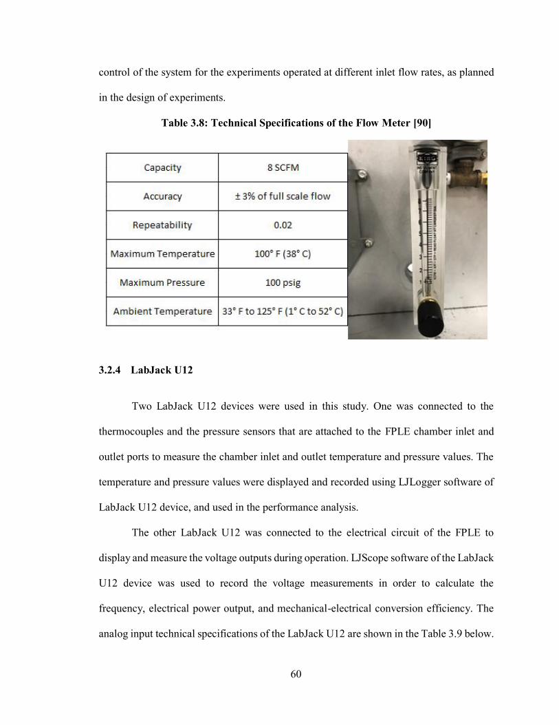
60
control of the system for the experiments operated at different inlet flow rates, as planned
in the design of experiments.
Table 3.8: Technical Specifications of the Flow Meter [90]
3.2.4 LabJack U12
Two LabJack U12 devices were used in this study. One was connected to the
thermocouples and the pressure sensors that are attached to the FPLE chamber inlet and
outlet ports to measure the chamber inlet and outlet temperature and pressure values. The
temperature and pressure values were displayed and recorded using LJLogger software of
LabJack U12 device, and used in the performance analysis.
The other LabJack U12 was connected to the electrical circuit of the FPLE to
display and measure the voltage outputs during operation. LJScope software of the LabJack
U12 device was used to record the voltage measurements in order to calculate the
frequency, electrical power output, and mechanical-electrical conversion efficiency. The
analog input technical specifications of the LabJack U12 are shown in the Table 3.9 below.

61
Table 3.9: Analog Inputs (AI0 – AI7) Technical Specifications of the LabJack U12 [91]
3.3 Thermodynamic Analysis
Thermodynamic analysis of the FPLE was necessary to investigate its performance.
The analysis was carried out by using the first and second laws of thermodynamics.
Conservation of mass, energy, and entropy were applied to analyze the performance of the
expander. The cylinder vessel of the FPLE was taken as the control volume for the analysis,
which has two inlets and outlets.
The conservation of energy for the control volume is:
𝑑E𝑐𝑣
𝑑𝑡= �� + �� + ��𝑖𝑛 (ℎ𝑖𝑛 +
𝑉𝑖𝑛2
2 + 𝑔𝑧𝑖𝑛) − ��𝑜𝑢𝑡 (ℎ𝑜𝑢𝑡 +
𝑉𝑜𝑢𝑡2
2 + 𝑔𝑧𝑜𝑢𝑡) (1)
where 𝑑Ecv
𝑑𝑡 is the rate of change in total internal energy (W), �� is the rate of heat transfer
(W), �� is the power output of the expander (W), ��𝑖𝑛/𝑜𝑢𝑡 is the mass flow rate of inlet and

62
outlet (kg/s). ℎ𝑖𝑛/𝑜𝑢𝑡, 𝑉𝑖𝑛/𝑜𝑢𝑡, and 𝑧𝑖𝑛/𝑜𝑢𝑡 represent enthalpy, velocity and the height level
of the air at the inlet and outlet (J/kg), respectively.
The conservation of mass for the control volume is:
𝑑m𝑐𝑣
𝑑𝑡= ��𝑖𝑛 − ��𝑜𝑢𝑡 (2)
The entropy balance and irreversibility equations for the control volume are:
𝑑S𝑐𝑣
𝑑𝑡= ��𝑖𝑛𝑠𝑖𝑛 − ��𝑜𝑢𝑡𝑠𝑜𝑢𝑡 +
��
𝑇𝑠+ ��𝑔𝑒𝑛 (3)
𝐼 = 𝑇𝑠 ��𝑔𝑒𝑛 (4)
where 𝑑S𝑐𝑣
𝑑𝑡 is the rate of change in total entropy of the system, 𝑠𝑖𝑛/𝑜𝑢𝑡 is the entropy of the
air at inlet and outlet, 𝑇𝑠 is the temperate of surroundings (equivalent to 293.15 K in this
study), and ��𝑔𝑒𝑛 is the entropy generated during the expansion process.
The volumetric efficiency of the FPLE can be defined as the ratio of the actual mass
flow rate to the mass flow rate of the ideal process. Therefore, during operation, the
volumetric efficiency is determined by:
𝜆 =𝑚𝑎
𝜌𝑎𝑉𝑑𝑓 (5)
where 𝜆 is the volumetric efficiency, 𝑚𝑎 , 𝜌𝑎, 𝑉𝑑, and 𝑓 represent air mass flow rate
supplied into one of the chambers, density of air evaluated at atmospheric conditions,
displacement volume, and frequency of the piston motion, respectively.
After a long-enough time, when the readings from the control volume did not
change, the operation of the expander can be assumed to be steady state. Therefore, steady
state conditions are assumed for this thermodynamic analysis. This assumption simplifies
the analysis and the change in any property with respect to time become equal to zero. As
is done by the previous study [77], heat losses are assumed to be negligible and the system

63
is assumed to be perfectly sealed. In addition, the changes in kinetic and potential energy
are negligibly small values and are equal to zero in this analysis. It was also assumed that
the volumetric flow rates into both chambers are equal and half of the total volumetric flow
rate. Since the air was considered as ideal gas, enthalpy properties of the air at the inlet and
outlet, and the change in the entropy of the air were calculated by the following equations:
ℎ = 𝑐𝑝𝑇 (6)
𝑠𝑖𝑛 − 𝑠𝑜𝑢𝑡 = 𝑐𝑝 ln (𝑇𝑜𝑢𝑡
𝑇𝑖𝑛) − 𝑅𝑎ln (
𝑃𝑜𝑢𝑡
𝑃𝑖𝑛) (7)
where 𝑐𝑝 is the specific heat of the air and taken as a constant value, 1.005 kJ/kg-K, T is
the temperature of the air. 𝑅𝑎 denotes the gas constant of air and taken as constant value,
0.2869 kJ/kg-K. After applying the assumptions into equation (1), (2), and (3) and
substituting the equation (6) and (7) into equation (1) and (3), respectively, the following
equations were obtained:
��𝑖𝑛 = ��𝑜𝑢𝑡 = 2��1,𝑖𝑛 = 2��2,𝑜𝑢𝑡 = 2��3,𝑖𝑛 = 2��4,𝑜𝑢𝑡 = �� = 𝜌𝑎��𝑖𝑛 (8)
��𝑜𝑢𝑡,𝑎 = ��
2𝑐𝑝{(𝑇1,𝑖𝑛 − 𝑇2,𝑜𝑢𝑡,𝑎) + (𝑇3,𝑖𝑛 − 𝑇4,𝑜𝑢𝑡,𝑎)} (9)
��𝑔𝑒𝑛 =��
2{[𝑐𝑝 ln (
𝑇2
𝑇1) − 𝑅𝑎ln (
𝑃2
𝑃1)] + [𝑐𝑝 ln (
𝑇4
𝑇3) − 𝑅𝑎 ln (
𝑃4
𝑃3)]} (10)
where the subscripts of 1, 2, 3, and 4 represent the states of the right chamber inlet, right
chamber outlet, left chamber inlet, and left chamber outlet, respectively. ��𝑖𝑛 represents the
total volumetric flow rate entering the control volume. ��𝑜𝑢𝑡,𝑎, 𝑇2,𝑜𝑢𝑡,𝑎, and 𝑇4,𝑜𝑢𝑡,𝑎 denote
actual expander work, and actual temperature at the outlets of the right and left chambers,
respectively. Finally, the isentropic efficiency for the control volume can be defined as the
ratio of the actual expander work output to the isentropic expander work output:
𝜂𝑠 =��𝑜𝑢𝑡,𝑎
��𝑜𝑢𝑡,𝑠 (11)

64
where 𝜂𝑠 is the isentropic efficiency, and ��𝑜𝑢𝑡,𝑠 is the isentropic work output of the
expander which is defined by:
��𝑜𝑢𝑡,𝑠 = ��
2𝑐𝑝{(𝑇1,𝑖𝑛 − 𝑇2,𝑜𝑢𝑡,𝑠) + (𝑇3,𝑖𝑛 − 𝑇4,𝑜𝑢𝑡,𝑠)} (12)
where 𝑇2,𝑜𝑢𝑡,𝑠 and 𝑇4,𝑜𝑢𝑡,𝑠 are the exit temperature of the air at, respectively, right and left
chambers for an isentropic expansion process and can be calculated by the following
relationship:
𝑇𝑜𝑢𝑡,𝑠 = 𝑇𝑖𝑛 (𝑃𝑜𝑢𝑡
𝑃𝑖𝑛)
𝑘−1
𝑘 (13)
where 𝑃𝑖𝑛 is the inlet chamber pressure, 𝑃𝑜𝑢𝑡 is the outlet chamber pressure. The
atmospheric pressure in this study was taken as 101.325 kPa, and 𝑘 is the specific heat ratio
and taken as a constant value, 1.401. Moreover, the average electrical power output is
calculated by the following relationship:
��𝑒,𝑎𝑣𝑔 =𝑉𝑅𝑀𝑆
𝑅2𝑒𝑞
(14)
where ��𝑒,𝑎𝑣𝑔, 𝑉𝑅𝑀𝑆, and 𝑅2𝑒𝑞 represent the average electrical power (W), RMS (root of
mean square) voltage (V), and the equivalent resistance (ohm), respectively. The RMS
voltage of a sample voltage data set of n value can be calculated using the following
relationship:
𝑉𝑅𝑀𝑆 = √𝑉12+𝑉2
2+𝑉3
2+...+𝑉𝑛2
𝑛 (15)
Mechanical-electrical conversion efficiency of the FPLE can be defined as the ratio
of the electrical power output (average) to the actual expander work. Therefore, during the
operation of the FPLE, the mechanical-electrical conversion efficiency, 𝜂𝑐, is defined as:
𝜂𝑐 =��𝑒,𝑎𝑣𝑔
��𝑜𝑢𝑡,𝑎 (16)

65
After achieving steady state operation of the FPLE, the inlet-outlet relationships
were evaluated in order to examine the operational characteristics and to identify the
conditions and trends for optimal performance of the FPLE. Table 3.10 presents the design
of experiments with the independent and dependent variables.

66
Table 3.10: Design of Experiments
Test
# Independent Variable Dependent Variables Controlled Variables
1
Inlet Air Pressure
(Range: 275.8-551.6
kPa in Absolute Units)
Actual Expander Work
Irreversibility
Isentropic Efficiency
Frequency
Volumetric Flow Rate
Volumetric Efficiency
RMS Voltage
Electrical Power Output
Conversion Efficiency
Inlet Air Temperature
Resistance Magnitude
2 Inlet Air Temperature
(Range: 50–90 °C)
Actual Expander Work
Irreversibility
Isentropic Efficiency
Frequency
Volumetric Efficiency
RMS Voltage
Electrical Power Output
Conversion Efficiency
Inlet Air Pressure
Resistance Magnitude
Volumetric Flow Rate
3
Resistance Magnitude
(Range: 0.667-8.333
Ohm)
Actual Expander Work
Irreversibility
Isentropic Efficiency
Frequency
Volumetric Efficiency
RMS Voltage
Electrical Power Output
Conversion Efficiency
Inlet Air Pressure
Inlet Temperature
Volumetric Flow Rate

67
3.3.1 Propagation of Error
Uncertainty analysis was performed to provide the accuracies of the calculated
parameters since the measurements from multiple instruments were included in the
calculation of the parameters. Standard deviations of the calculated parameters were
determined by using the exact formula for propagation of error [92]:
𝜎𝑥2 = (
𝛿𝑥
𝛿𝑎)
2
𝜎𝑎2 + (
𝛿𝑥
𝛿𝑏)
2
𝜎𝑏2 + (
𝛿𝑥
𝛿𝑐)
2
𝜎𝑐2 (17)
where x is defined as the parameter desired (e.g., 𝜂𝑠, ��𝑜𝑢𝑡,𝑠, ��𝑔𝑒𝑛, etc.) and is function of
a, b, and c. The standard deviations of x, a, b, and c, are represented by 𝜎𝑥, 𝜎𝑎, 𝜎𝑏, and 𝜎𝑐,
respectively.

68
4 Results and Discussion
The steady state operation of the Free-Piston Linear Expander was successfully
achieved after applying the forementioned modifications. The experiments were conducted
at the University of North Florida’s College of Computing, Engineering & Construction’s
Mechanical Engineering Energy Efficiency Laboratory in order to analyze the performance
of the FPLE by varying the inlet pressure and inlet temperature of the air, and the electrical
resistance, connected as the output load to the expander. The thermodynamic and voltage
data recordings were started after running each experiment. A range in the temperature
readings where the readings were steady was chosen as the steady state region. The average
values of the thermodynamic and voltage data in the steady state regions were used as the
steady state properties for the analysis of each experiment. The Figure 4.1 presents an
example for the selection of the steady state region of an experiment with the inlet air
pressure and temperature, and the resistance magnitude of 413.7 kPa, 50 °C, and 0.667
ohm, respectively. The bars labeled with 1500 and 1680 in Figure 4.1 indicates the
boundaries of the steady state region. The 1500 and the 1680 labels are the time since the
data recording started.
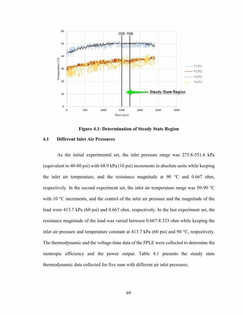
69
Figure 4.1: Determination of Steady State Region
4.1 Different Inlet Air Pressures
As the initial experimental set, the inlet pressure range was 275.8-551.6 kPa
(equivalent to 40-80 psi) with 68.9 kPa (10 psi) increments in absolute units while keeping
the inlet air temperature, and the resistance magnitude at 90 °C and 0.667 ohm,
respectively. In the second experiment set, the inlet air temperature range was 50-90 °C
with 10 °C increments, and the control of the inlet air pressure and the magnitude of the
load were 413.7 kPa (60 psi) and 0.667 ohm, respectively. In the last experiment set, the
resistance magnitude of the load was varied between 0.667-8.333 ohm while keeping the
inlet air pressure and temperature constant at 413.7 kPa (60 psi) and 90 °C, respectively.
The thermodynamic and the voltage-time data of the FPLE were collected to determine the
isentropic efficiency and the power output. Table 4.1 presents the steady state
thermodynamic data collected for five runs with different air inlet pressures.
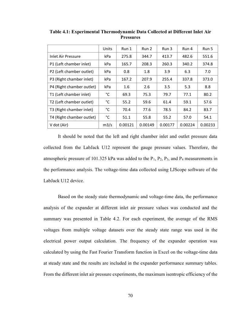
70
Table 4.1: Experimental Thermodynamic Data Collected at Different Inlet Air Pressures
Units Run 1 Run 2 Run 3 Run 4 Run 5
Inlet Air Pressure kPa 275.8 344.7 413.7 482.6 551.6
P1 (Left chamber inlet) kPa 165.7 208.3 260.3 340.2 374.8
P2 (Left chamber outlet) kPa 0.8 1.8 3.9 6.3 7.0
P3 (Right chamber inlet) kPa 167.2 207.9 255.4 337.8 373.0
P4 (Right chamber outlet) kPa 1.6 2.6 3.5 5.3 8.8
T1 (Left chamber inlet) °C 69.3 75.3 79.7 77.1 80.2
T2 (Left chamber outlet) °C 55.2 59.6 61.4 59.1 57.6
T3 (Right chamber inlet) °C 70.4 77.6 78.5 84.2 83.7
T4 (Right chamber outlet) °C 51.1 55.8 55.2 57.0 54.1
V dot (Air) m3/s 0.00121 0.00149 0.00177 0.00224 0.00233
It should be noted that the left and right chamber inlet and outlet pressure data
collected from the LabJack U12 represent the gauge pressure values. Therefore, the
atmospheric pressure of 101.325 kPa was added to the P1, P2, P3, and P4 measurements in
the performance analysis. The voltage-time data collected using LJScope software of the
LabJack U12 device.
Based on the steady state thermodynamic and voltage-time data, the performance
analysis of the expander at different inlet air pressure values was conducted and the
summary was presented in Table 4.2. For each experiment, the average of the RMS
voltages from multiple voltage datasets over the steady state range was used in the
electrical power output calculation. The frequency of the expander operation was
calculated by using the Fast Fourier Transform function in Excel on the voltage-time data
at steady state and the results are included in the expander performance summary tables.
From the different inlet air pressure experiments, the maximum isentropic efficiency of the
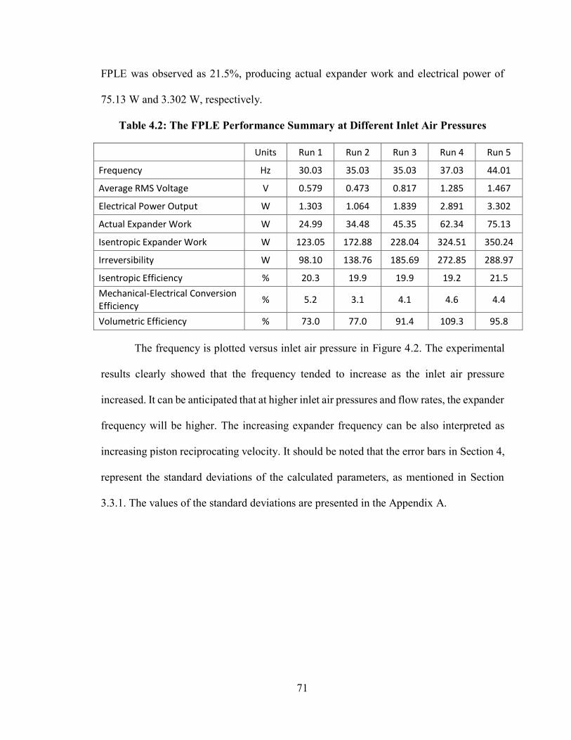
71
FPLE was observed as 21.5%, producing actual expander work and electrical power of
75.13 W and 3.302 W, respectively.
Table 4.2: The FPLE Performance Summary at Different Inlet Air Pressures
Units Run 1 Run 2 Run 3 Run 4 Run 5
Frequency Hz 30.03 35.03 35.03 37.03 44.01
Average RMS Voltage V 0.579 0.473 0.817 1.285 1.467
Electrical Power Output W 1.303 1.064 1.839 2.891 3.302
Actual Expander Work W 24.99 34.48 45.35 62.34 75.13
Isentropic Expander Work W 123.05 172.88 228.04 324.51 350.24
Irreversibility W 98.10 138.76 185.69 272.85 288.97
Isentropic Efficiency % 20.3 19.9 19.9 19.2 21.5
Mechanical-Electrical Conversion Efficiency
% 5.2 3.1 4.1 4.6 4.4
Volumetric Efficiency % 73.0 77.0 91.4 109.3 95.8
The frequency is plotted versus inlet air pressure in Figure 4.2. The experimental
results clearly showed that the frequency tended to increase as the inlet air pressure
increased. It can be anticipated that at higher inlet air pressures and flow rates, the expander
frequency will be higher. The increasing expander frequency can be also interpreted as
increasing piston reciprocating velocity. It should be noted that the error bars in Section 4,
represent the standard deviations of the calculated parameters, as mentioned in Section
3.3.1. The values of the standard deviations are presented in the Appendix A.
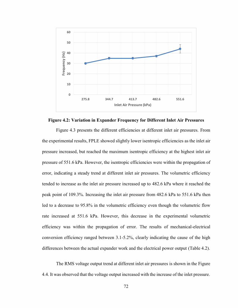
72
Figure 4.2: Variation in Expander Frequency for Different Inlet Air Pressures
Figure 4.3 presents the different efficiencies at different inlet air pressures. From
the experimental results, FPLE showed slightly lower isentropic efficiencies as the inlet air
pressure increased, but reached the maximum isentropic efficiency at the highest inlet air
pressure of 551.6 kPa. However, the isentropic efficiencies were within the propagation of
error, indicating a steady trend at different inlet air pressures. The volumetric efficiency
tended to increase as the inlet air pressure increased up to 482.6 kPa where it reached the
peak point of 109.3%. Increasing the inlet air pressure from 482.6 kPa to 551.6 kPa then
led to a decrease to 95.8% in the volumetric efficiency even though the volumetric flow
rate increased at 551.6 kPa. However, this decrease in the experimental volumetric
efficiency was within the propagation of error. The results of mechanical-electrical
conversion efficiency ranged between 3.1-5.2%, clearly indicating the cause of the high
differences between the actual expander work and the electrical power output (Table 4.2).
The RMS voltage output trend at different inlet air pressures is shown in the Figure
4.4. It was observed that the voltage output increased with the increase of the inlet pressure.
0
10
20
30
40
50
60
275.8 344.7 413.7 482.6 551.6
Freq
uen
cy (
Hz)
Inlet Air Pressure (kPa)
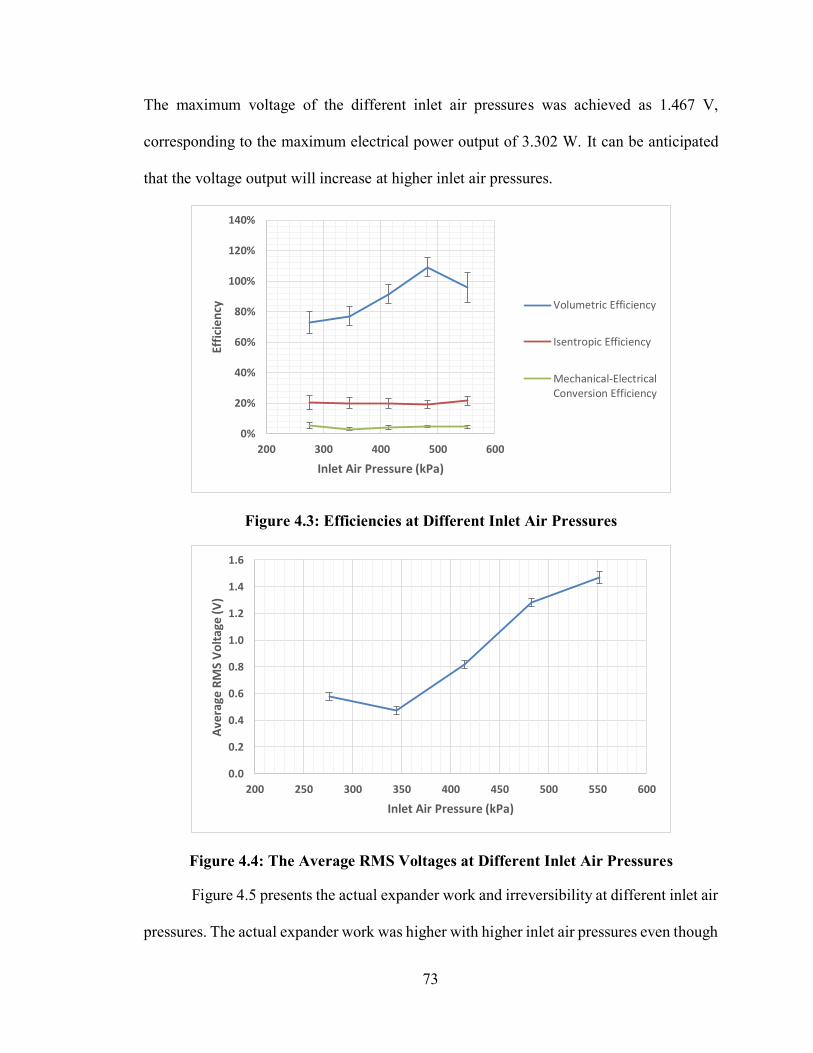
73
The maximum voltage of the different inlet air pressures was achieved as 1.467 V,
corresponding to the maximum electrical power output of 3.302 W. It can be anticipated
that the voltage output will increase at higher inlet air pressures.
Figure 4.3: Efficiencies at Different Inlet Air Pressures
Figure 4.4: The Average RMS Voltages at Different Inlet Air Pressures
Figure 4.5 presents the actual expander work and irreversibility at different inlet air
pressures. The actual expander work was higher with higher inlet air pressures even though
0%
20%
40%
60%
80%
100%
120%
140%
200 300 400 500 600
Effi
cien
cy
Inlet Air Pressure (kPa)
Volumetric Efficiency
Isentropic Efficiency
Mechanical-ElectricalConversion Efficiency
0.0
0.2
0.4
0.6
0.8
1.0
1.2
1.4
1.6
200 250 300 350 400 450 500 550 600
Ave
rage
RM
S V
olt
age
(V)
Inlet Air Pressure (kPa)
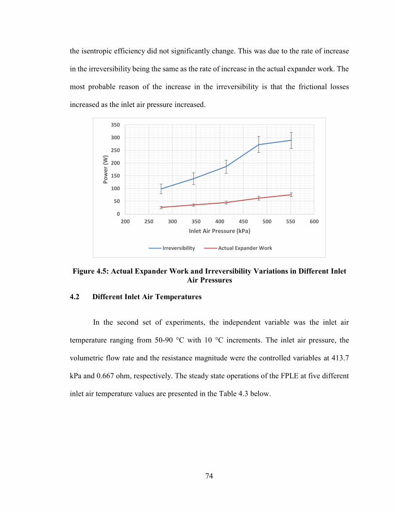
74
the isentropic efficiency did not significantly change. This was due to the rate of increase
in the irreversibility being the same as the rate of increase in the actual expander work. The
most probable reason of the increase in the irreversibility is that the frictional losses
increased as the inlet air pressure increased.
Figure 4.5: Actual Expander Work and Irreversibility Variations in Different Inlet Air Pressures
4.2 Different Inlet Air Temperatures
In the second set of experiments, the independent variable was the inlet air
temperature ranging from 50-90 °C with 10 °C increments. The inlet air pressure, the
volumetric flow rate and the resistance magnitude were the controlled variables at 413.7
kPa and 0.667 ohm, respectively. The steady state operations of the FPLE at five different
inlet air temperature values are presented in the Table 4.3 below.
0
50
100
150
200
250
300
350
200 250 300 350 400 450 500 550 600
Po
wer
(W
)
Inlet Air Pressure (kPa)
Irreversibility Actual Expander Work
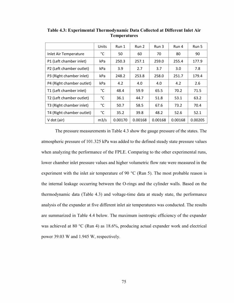
75
Table 4.3: Experimental Thermodynamic Data Collected at Different Inlet Air Temperatures
Units Run 1 Run 2 Run 3 Run 4 Run 5
Inlet Air Temperature °C 50 60 70 80 90
P1 (Left chamber inlet) kPa 250.3 257.1 259.0 255.4 177.9
P2 (Left chamber outlet) kPa 3.9 2.7 3.7 3.0 7.8
P3 (Right chamber inlet) kPa 248.2 253.8 258.0 251.7 179.4
P4 (Right chamber outlet) kPa 4.2 4.0 4.0 4.2 2.6
T1 (Left chamber inlet) °C 48.4 59.9 65.5 70.2 71.5
T2 (Left chamber outlet) °C 36.1 44.7 51.8 53.1 63.2
T3 (Right chamber inlet) °C 50.7 58.5 67.6 73.2 70.4
T4 (Right chamber outlet) °C 35.2 39.8 48.2 52.6 52.1
V dot (air) m3/s 0.00170 0.00168 0.00168 0.00168 0.00205
The pressure measurements in Table 4.3 show the gauge pressure of the states. The
atmospheric pressure of 101.325 kPa was added to the defined steady state pressure values
when analyzing the performance of the FPLE. Comparing to the other experimental runs,
lower chamber inlet pressure values and higher volumetric flow rate were measured in the
experiment with the inlet air temperature of 90 °C (Run 5). The most probable reason is
the internal leakage occurring between the O-rings and the cylinder walls. Based on the
thermodynamic data (Table 4.3) and voltage-time data at steady state, the performance
analysis of the expander at five different inlet air temperatures was conducted. The results
are summarized in Table 4.4 below. The maximum isentropic efficiency of the expander
was achieved at 80 °C (Run 4) as 18.6%, producing actual expander work and electrical
power 39.03 W and 1.945 W, respectively.
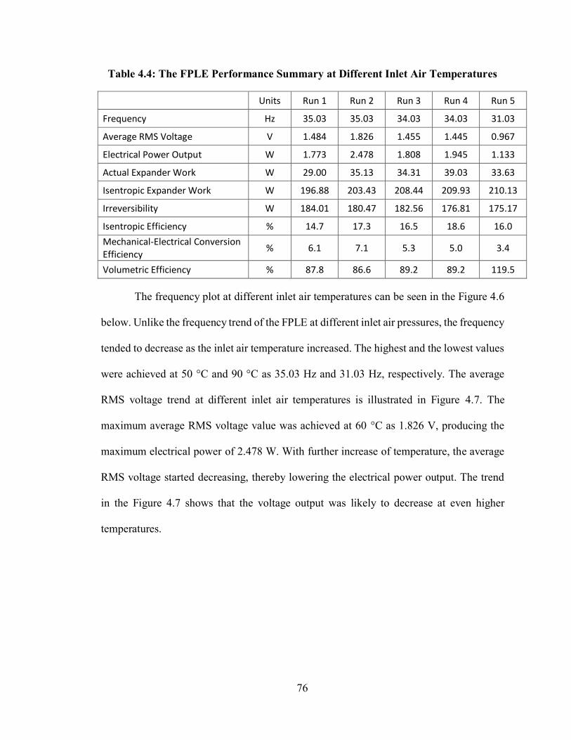
76
Table 4.4: The FPLE Performance Summary at Different Inlet Air Temperatures
Units Run 1 Run 2 Run 3 Run 4 Run 5
Frequency Hz 35.03 35.03 34.03 34.03 31.03
Average RMS Voltage V 1.484 1.826 1.455 1.445 0.967
Electrical Power Output W 1.773 2.478 1.808 1.945 1.133
Actual Expander Work W 29.00 35.13 34.31 39.03 33.63
Isentropic Expander Work W 196.88 203.43 208.44 209.93 210.13
Irreversibility W 184.01 180.47 182.56 176.81 175.17
Isentropic Efficiency % 14.7 17.3 16.5 18.6 16.0
Mechanical-Electrical Conversion Efficiency
% 6.1 7.1 5.3 5.0 3.4
Volumetric Efficiency % 87.8 86.6 89.2 89.2 119.5
The frequency plot at different inlet air temperatures can be seen in the Figure 4.6
below. Unlike the frequency trend of the FPLE at different inlet air pressures, the frequency
tended to decrease as the inlet air temperature increased. The highest and the lowest values
were achieved at 50 °C and 90 °C as 35.03 Hz and 31.03 Hz, respectively. The average
RMS voltage trend at different inlet air temperatures is illustrated in Figure 4.7. The
maximum average RMS voltage value was achieved at 60 °C as 1.826 V, producing the
maximum electrical power of 2.478 W. With further increase of temperature, the average
RMS voltage started decreasing, thereby lowering the electrical power output. The trend
in the Figure 4.7 shows that the voltage output was likely to decrease at even higher
temperatures.

77
Figure 4.6: Variation of Expander Frequency for Different Inlet Air Temperatures
Figure 4.7: The Average RMS Voltages at Different Inlet Air Temperatures
The trends of the efficiencies at different inlet air temperatures are shown in Figure
4.8. For different inlet air temperatures, the isentropic efficiency ranged between 14.7%
and 18.6%. The maximum electrical power of 2.478 W was produced during the second
run (inlet air temperature of 60 °C) while the isentropic efficiency was 17.3%. The reason
for this is that the mechanical-electrical conversion efficiency reached its peak value, 7.1%,
27
28
29
30
31
32
33
34
35
36
37
50 60 70 80 90
Freq
uen
cy (
Hz)
Temperature (°C)
0.0
0.2
0.4
0.6
0.8
1.0
1.2
1.4
1.6
1.8
2.0
40 50 60 70 80 90 100
Ave
rage
RM
S V
olt
age
(V)
Temperature (°C)

78
for the inlet air temperature of 60 °C, allowing the production of more electric power even
though the actual expander work was not at its highest value. In this same experiment, the
FPLE showed the lowest volumetric efficiency of 86.6%. With the further increase of the
inlet air temperature, the volumetric efficiency was observed to increase, reaching to its
highest value of 119.5% at the inlet air temperature of 90 °C. From 50 °C to 80 °C, the
volumetric efficiency showed slight changes, which were found to be within the
propagation of error. On contrary, at the inlet air temperature of 90 °C, a significant
increase in the volumetric efficiency was observed. This can be connected to an excessive
internal leakage occurring between the piston O-rings and the cylinder walls, which
supports the hypothesis stated previously regarding the low chamber inlet pressures and
high volumetric flow rate measurements for the inlet air temperature of 90 °C (Table 4.3).
The mechanical-electrical conversion efficiency, on the other hand, tended to decrease as
the inlet air temperature increased from 60 °C to 90 °C. Moreover, the trends in Figure 4.8
clearly shows that the volumetric efficiency will likely increase at even higher
temperatures, whereas the mechanical-electrical conversion efficiency can be expected to
further decrease.

79
Figure 4.8: Efficiencies at Different Inlet Air Temperatures
Figure 4.9 presents the trends of the actual expander work and the irreversibility of
the FPLE at different inlet air temperatures. Actual expander work tended to increase as
the inlet air temperature increased, reaching at its peak value of 39.03 W with an inlet air
temperature of 80 °C. Increasing the temperature from 80 °C to 90 °C resulted in a decrease
in the actual expander work. This was likely due to excessive internal leakage, which also
explains why the chamber inlet pressure values were low and the volume flow rate was
high for 90 °C. Internal leakage was possible between the O-rings and the cylinder wall
that can cause the leaking of air from one chamber to another and/or inlet to outlet. The
irreversibility, on the other hand, had a tendency to decrease as the inlet air temperature
increased. It can be also seen from Figure 4.9 that the irreversibility was likely to further
decrease at even higher inlet air temperatures.
0%
20%
40%
60%
80%
100%
120%
140%
40 50 60 70 80 90 100
Effi
cien
cy
Temperature (°C)
Volumetric Efficiency
Isentropic Efficiency
Mechanical-ElectricalConversion Efficiency

80
Figure 4.9: Actual Expander Work and Irreversibility Variations in Different Inlet Air Temperatures
4.3 Different Resistance Magnitudes
In the third and last set of experiments, the inlet air temperature and the pressure
values were controlled at 90 °C and 413.7 kPa, respectively, while varying the magnitude
of the load connected to the FPLE from 0.667 up to 8.333 ohms. Four experiments with
different resistance magnitudes were performed in order to analyze the outputs. The steady
state thermodynamic properties obtained from the data of performed experiments are
presented in Table 4.5 below.
0
50
100
150
200
250
40 50 60 70 80 90 100
Po
wer
(W
)
Inlet Air Temperature (°C)
Irreversibility (W) Actual Expander Work (W)
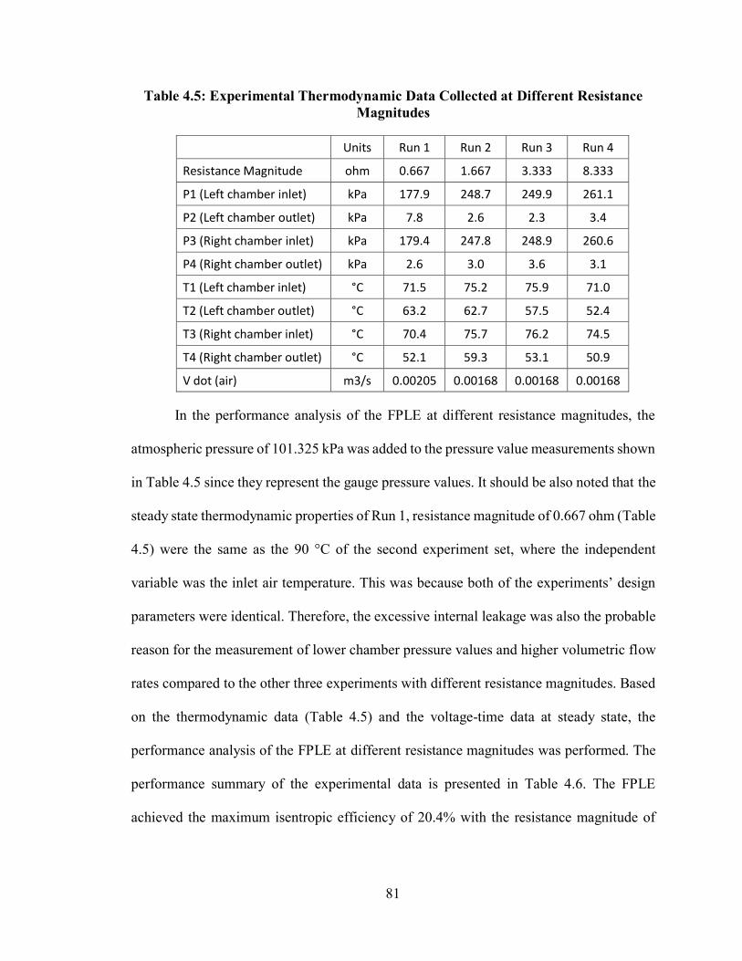
81
Table 4.5: Experimental Thermodynamic Data Collected at Different Resistance Magnitudes
Units Run 1 Run 2 Run 3 Run 4
Resistance Magnitude ohm 0.667 1.667 3.333 8.333
P1 (Left chamber inlet) kPa 177.9 248.7 249.9 261.1
P2 (Left chamber outlet) kPa 7.8 2.6 2.3 3.4
P3 (Right chamber inlet) kPa 179.4 247.8 248.9 260.6
P4 (Right chamber outlet) kPa 2.6 3.0 3.6 3.1
T1 (Left chamber inlet) °C 71.5 75.2 75.9 71.0
T2 (Left chamber outlet) °C 63.2 62.7 57.5 52.4
T3 (Right chamber inlet) °C 70.4 75.7 76.2 74.5
T4 (Right chamber outlet) °C 52.1 59.3 53.1 50.9
V dot (air) m3/s 0.00205 0.00168 0.00168 0.00168
In the performance analysis of the FPLE at different resistance magnitudes, the
atmospheric pressure of 101.325 kPa was added to the pressure value measurements shown
in Table 4.5 since they represent the gauge pressure values. It should be also noted that the
steady state thermodynamic properties of Run 1, resistance magnitude of 0.667 ohm (Table
4.5) were the same as the 90 °C of the second experiment set, where the independent
variable was the inlet air temperature. This was because both of the experiments’ design
parameters were identical. Therefore, the excessive internal leakage was also the probable
reason for the measurement of lower chamber pressure values and higher volumetric flow
rates compared to the other three experiments with different resistance magnitudes. Based
on the thermodynamic data (Table 4.5) and the voltage-time data at steady state, the
performance analysis of the FPLE at different resistance magnitudes was performed. The
performance summary of the experimental data is presented in Table 4.6. The FPLE
achieved the maximum isentropic efficiency of 20.4% with the resistance magnitude of

82
8.333 ohm, producing actual expander work and electrical power of 43.67 W and 0.033 W,
respectively.
Table 4.6: The FPLE Performance Summary at Different Resistance Magnitudes
Units Run 1 Run 2 Run 3 Run 4
Frequency Hz 31.03 38.03 37.03 34.03
Average RMS Voltage W 0.503 0.642 1.488 2.320
Electrical Power Output W 1.133 0.231 0.134 0.033
Actual Expander Work W 33.63 29.88 42.89 43.67
Isentropic Expander Work W 210.13 211.13 211.73 213.98
Irreversibility % 175.17 183.96 172.77 176.82
Isentropic Efficiency % 16.0 14.2 20.3 20.4
Mechanical-Electrical Conversion Efficiency
% 3.4 0.8 0.3 0.1
Volumetric Efficiency % 119.5 79.8 81.9 89.2
Figure 4.10 presents the average RMS voltage trend versus different load
magnitudes. The average RMS voltage was observed to increase as the resistance
magnitude increased. The maximum average RMS voltage was achieved as 2.320 V at the
resistance magnitude of 8.333 ohm and it can be anticipated that further increase in the
resistance magnitude, the higher the average RMS voltage. The electrical power, unlike the
voltage trend, was observed to be decreasing as the load magnitude increased. The
maximum electric power was achieved at the load magnitude of 0.667 ohm as 1.133 W.
The Figure 4.11 demonstrates the frequency trend versus different resistance magnitudes.
The FPLE showed the maximum frequency of 38.02 Hz for 1.667 ohm. The frequency
showed an increasing and then decreasing trend with increasing resistance.
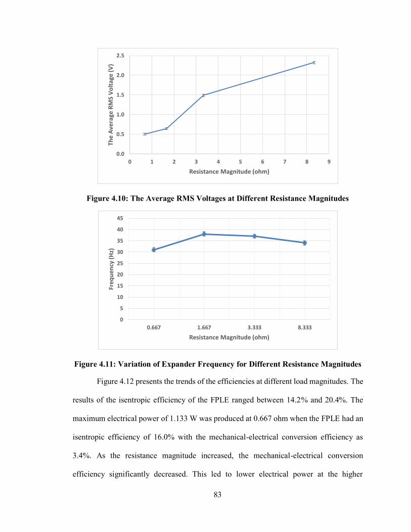
83
Figure 4.10: The Average RMS Voltages at Different Resistance Magnitudes
Figure 4.11: Variation of Expander Frequency for Different Resistance Magnitudes
Figure 4.12 presents the trends of the efficiencies at different load magnitudes. The
results of the isentropic efficiency of the FPLE ranged between 14.2% and 20.4%. The
maximum electrical power of 1.133 W was produced at 0.667 ohm when the FPLE had an
isentropic efficiency of 16.0% with the mechanical-electrical conversion efficiency as
3.4%. As the resistance magnitude increased, the mechanical-electrical conversion
efficiency significantly decreased. This led to lower electrical power at the higher
0.0
0.5
1.0
1.5
2.0
2.5
0 1 2 3 4 5 6 7 8 9
The
Ave
rage
RM
S V
olt
age
(V)
Resistance Magnitude (ohm)
0
5
10
15
20
25
30
35
40
45
0.667 1.667 3.333 8.333
Freq
uen
cy (
Hz)
Resistance Magnitude (ohm)

84
resistance magnitudes even though the isentropic efficiency increased. At 0.667 ohm and
1.667 ohm, the isentropic efficiency did not change significantly, remaining within the
propagation of error. Increasing the resistance magnitude from 1.667 ohm to 3.333 ohm
resulted in an increase in the isentropic efficiency, achieving 20.3%. As the load was
further increased from 3.333 ohm to 8.333 ohm, the expander reached the peak value of
isentropic efficiency, 20.4%. The peak value of the volumetric efficiency was observed at
the resistance magnitude of 0.667 ohm as 119.5%, then, it decreased to 79.8% for 1.667
ohm. The reason behind the peak volumetric efficiency of 119.5% can be connected to the
possible excessive internal leakages taking place at the resistance magnitude of 0.667 ohm.
As the internal leakage increased, more air was supplied to the system. This will lead to an
increase in the volumetric flow rate and the volumetric efficiency. From 1.667 ohm to
3.333 ohm and then to 8.333 ohm, the volumetric efficiency had a tendency to increase,
achieving 79.8%, 81.9% and 89.2%, respectively. From this trend, it can be anticipated that
higher volumetric efficiencies than 89.2% can be achieved at even higher resistance
magnitudes.

85
Figure 4.12: Efficiencies at Different Resistance Magnitudes
Figure 4.13 below displays the trends of the actual expander work and the
irreversibility of the FPLE under different loads. The FPLE achieved the maximum actual
expander work of 43.67 W in the Run 4 with the resistance magnitude of 8.333 ohm. From
0.667 ohm to 1.667 ohm, a decrease in the actual expander work was observed from 33.63
W to 29.88 W. Thereafter, from 1.667 ohm to 8.333 ohm, the actual expander work had a
tendency to increase as the resistance magnitude increased; indicating that with further
increase in the resistance magnitude, the actual expander work is likely to increase. The
maximum irreversibility was observed as 183.96 W at the resistance magnitude of 1.667
ohm. Apart from that, no significant change was obtained in terms of irreversibility as the
resistance magnitude increased.
0%
20%
40%
60%
80%
100%
120%
140%
0 1 2 3 4 5 6 7 8 9
Effi
cien
cy
Resistance Magnitude (ohm)
Volumetric Efficiency
Isentropic Efficiency
Mechanical-ElectricalConversion Efficiency
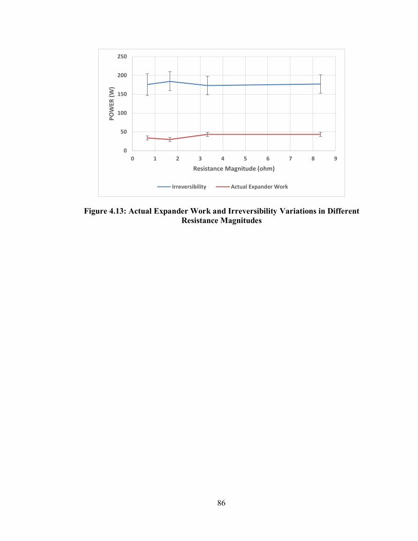
86
Figure 4.13: Actual Expander Work and Irreversibility Variations in Different Resistance Magnitudes
0
50
100
150
200
250
0 1 2 3 4 5 6 7 8 9
PO
WER
(W
)
Resistance Magnitude (ohm)
Irreversibility Actual Expander Work

87
5 Conclusion
The previous design of the Free-Piston Linear expander (FPLE) was modified and
the long-term steady state operation of the FPLE was successfully achieved. Three different
sets of experiments were performed in order to analyze the performance of the FPLE with
varying inlet air pressure, inlet air temperature, and resistance magnitude.
The frequency output of the FPLE had a tendency to increase as the inlet air
pressure increased while increasing the inlet air temperature resulted in the decrease of the
frequency. At the different resistance magnitudes, the frequency reached its peak value of
38.03 Hz. The maximum frequency in all the experiments was achieved as 44.01 Hz at an
inlet air pressure and temperature, and the resistance magnitude of 551.6 kPa, 90 °C, and
0.667 ohm, respectively. It can be concluded from the trends that the frequency will likely
increase at even higher inlet air pressures and even lower temperatures at a load magnitude
of 1.667 ohm.
The FPLE produced the maximum average RMS voltage of 2.320 V at the inlet air
pressure, inlet air temperature and the resistance magnitude of 413.7 kPa, 90 °C, and 8.333
ohm, respectively. It can be anticipated from the trends that the voltage is likely to increase
at even higher inlet air pressures and resistance magnitudes with an optimum inlet air
temperature of 60 °C. Electrical power output had similar trends to the RMS voltage with
the only difference being that increasing the resistance magnitude significantly decreased
the electrical power production.

88
The results showed that the maximum isentropic efficiency of the FPLE was
achieved as 21.5%, producing maximum actual expander work and maximum electrical
power of 75.13 W and 3.302 W, respectively. The maximum isentropic efficiency, at the
different inlet air temperature experiments, was observed at the inlet air temperature of 80
°C. It can be concluded from the trends that the isentropic efficiency results remained
within the propagation of error with the variation of resistance magnitudes. The
mechanical-electrical conversion efficiency results ranged between 0.1%-7.1%, clearly
indicating the cause of the large differences between the actual expander work and the
electrical power output.
Volumetric efficiency reached its optimum point at the inlet air pressure of 482.6
kPa during the different inlet air pressure experiments. Varying the inlet air temperature
did not significantly (within the propagation of error) change the volumetric efficiency,
except for 90 °C. A relatively high volumetric efficiency was observed for 90 °C and 0.667
ohm. The most probable reason was an excessive internal leakage occurring between the
piston O-rings and the cylinder walls. The measurements of relatively low chamber inlet
pressures and high volumetric flow rates at these 90 °C and 0.667 ohm experiments also
supported this hypothesis.
Actual expander work of the FPLE increased as the inlet air pressure increased,
reaching its maximum value at the inlet air pressure of 551.6 kPa. Increasing the resistance
magnitude from 1.667 ohm up to 8.333 ohm also resulted in higher actual expander work
outputs. It can be concluded that the actual expander work will likely be higher at higher
inlet air pressures and resistance magnitudes, noting that the optimum temperature for
actual expander work was 80 °C. Irreversibility, on the other hand, showed a tendency to

89
increase as the inlet air pressure increased, and to decrease as the inlet air temperature
increased. However, the changes in the irreversibility at different inlet air temperatures
were within the propagation of error. Varying the resistance magnitude did not significantly
change the irreversibility.
In the literature, turbines, scroll expanders, screw expanders, rotary vane
expanders, gerotor, reciprocating piston expanders, and rotary piston expanders were found
to achieve isentropic efficiencies of up to 85%, 50-89%, up to 76%, 23-73%, up to 85%,
up to 70%, and 28-77%, respectively. In this study, the maximum isentropic efficiency of
the FPLE was 21.5%. It should be noted this was the first iteration of this FPLE design.
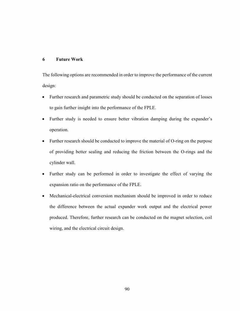
90
6 Future Work
The following options are recommended in order to improve the performance of the current
design:
Further research and parametric study should be conducted on the separation of losses
to gain further insight into the performance of the FPLE.
Further study is needed to ensure better vibration damping during the expander’s
operation.
Further research should be conducted to improve the material of O-ring on the purpose
of providing better sealing and reducing the friction between the O-rings and the
cylinder wall.
Further study can be performed in order to investigate the effect of varying the
expansion ratio on the performance of the FPLE.
Mechanical-electrical conversion mechanism should be improved in order to reduce
the difference between the actual expander work output and the electrical power
produced. Therefore, further research can be conducted on the magnet selection, coil
wiring, and the electrical circuit design.
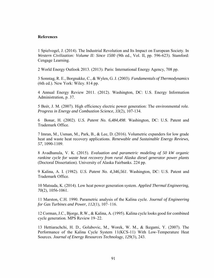
91
References
1 Spielvogel, J. (2014). The Industrial Revolution and Its Impact on European Society. In Western Civilization: Volume II: Since 1500 (9th ed., Vol. II, pp. 596-623). Stamford: Cengage Learning.
2 World Energy Outlook 2013. (2013). Paris: International Energy Agency, 708 pp.
3 Sonntag, R. E., Borgnakke, C., & Wylen, G. J. (2003). Fundamentals of Thermodynamics (6th ed.). New York: Wiley. 814 pp.
4 Annual Energy Review 2011. (2012). Washington, DC: U.S. Energy Information Administration, p. 37.
5 Beér, J. M. (2007). High efficiency electric power generation: The environmental role. Progress in Energy and Combustion Science, 33(2), 107-134.
6 Bonar, H. (2002). U.S. Patent No. 6,484,498. Washington, DC: U.S. Patent and Trademark Office.
7 Imran, M., Usman, M., Park, B., & Lee, D. (2016). Volumetric expanders for low grade heat and waste heat recovery applications. Renewable and Sustainable Energy Reviews,
57, 1090-1109.
8 Avadhanula, V. K. (2015). Evaluation and parametric modeling of 50 kW organic
rankine cycle for waste heat recovery from rural Alaska diesel generator power plants (Doctoral Dissertation). University of Alaska Fairbanks. 224 pp.
9 Kalina, A. I. (1982). U.S. Patent No. 4,346,561. Washington, DC: U.S. Patent and Trademark Office.
10 Matsuda, K. (2014). Low heat power generation system. Applied Thermal Engineering,
70(2), 1056-1061.
11 Marston, C.H. 1990. Parametric analysis of the Kalina cycle. Journal of Engineering
for Gas Turbines and Power, 112(1), 107–116.
12 Corman, J.C., Bjorge, R.W., & Kalina, A. (1995). Kalina cycle looks good for combined cycle generation. MPS Review 19–22.
13 Hettiarachchi, H. D., Golubovic, M., Worek, W. M., & Ikegami, Y. (2007). The Performance of the Kalina Cycle System 11(KCS-11) With Low-Temperature Heat Sources. Journal of Energy Resources Technology, 129(3), 243.

92
14 Park, Y. M. & Sonntag, R. E. (1990). A preliminary study of the kalina power cycle in connection with a combined cycle system. International Journal of Energy Research,
14(2), 153-162.
15 Harada, K. J. (2010). Development of a Small Scale Scroll Expander (Master’s Thesis). Oregon State University. 142 pp.
16 Quoilin, S. (2007). Experimental Study and Modeling of a Low Temperature Rankine
Cycle for Small Scale Cogeneration (Master’s Thesis). University of Liege. 129 pp.
17 Kinnaly, E. B. & Nuszkowski, J. (2015). Volumetric Rotary Expansion Machines – A Review. Jacksonville: University of North Florida.
18 Fraas, A. P. (1982). Engineering evaluation of energy systems. New York: McGraw-Hill. 702 pp.
19 Yang, J. L., Ma, Y. T., Li, M. X., & Guan, H. Q. (2005). Exergy analysis of transcritical carbon dioxide refrigeration cycle with an expander. Energy, 30(7), 1162-1175.
20 Chen, Y., Lundqvist, P., Johansson, A., & Platell, P. (2006). A comparative study of the carbon dioxide transcritical power cycle compared with an organic rankine cycle with R123 as working fluid in waste heat recovery. Applied Thermal Engineering, 26(17-18), 2142-2147.
21 Baek, J., Groll, E., & Lawless, P. (2005). Piston-cylinder work producing expansion device in a transcritical carbon dioxide cycle. Part I: Experimental investigation. International Journal of Refrigeration, 28(2), 141-151.
22 Kongtragool, B. & Wongwises, S. (2007). Performance of low-temperature differential Stirling engines. Renewable Energy, 32(4), 547-566
23 Cengel, Y. A. & Boles, M. A. (2006). Thermodynamics: An engineering approach (5th ed.). Boston: McGraw-Hill. 963 pp.
24 Tarique, M. A. (2011). Experimental investigation of scroll based organic Rankine
systems (Master’s Thesis). University of Ontario Institute of Technology. 186 pp.
25 Çinar, C. & Karabulut, H. (2005). Manufacturing and testing of a gamma type Stirling engine. Renewable Energy, 30(1), 57-66.
26 Thombare, D. & Verma, S. (2008). Technological development in the Stirling cycle engines. Renewable and Sustainable Energy Reviews, 12(1), 1-38.
27 Yang, B., Ahuja, H., & Tran, T. (2008). Review Article: Thermoelectric Technology Assessment: Application to Air Conditioning and Refrigeration. HVAC&R Res. UHVC
HVAC&R Research, 14(5), 635-653.

93
28 Oralli, E. (2010). Conversion of a scroll compressor to an expander for organic Rankine
cycle: Modeling and analysis (Master’s thesis). University of Ontario Institute of Technology. 162 pp.
29 Kumar, S., Heister, S. D., Xu, X., Salvador, J. R., & Meisner, G. P. (2013). Thermoelectric Generators for Automotive Waste Heat Recovery Systems Part I: Numerical Modeling and Baseline Model Analysis. Journal of Electronic Materials, 42(4), 665-674.
30 Aphornratana, S. & Sriveerakul, T. (2010). Analysis of a combined Rankine–vapour–compression refrigeration cycle. Energy Conversion and Management, 51(12), 2557-2564.
31 Lemort, V., Quoilin, S., Cuevas, C., & Lebrun, J. (2009). Testing and modeling a scroll expander integrated into an Organic Rankine Cycle. Applied Thermal Engineering, 29(14-15), 3094-3102.
32 Desideri, A., Gusev, S., Broek, M. V., Lemort, V., & Quoilin, S. (2016). Experimental comparison of organic fluids for low temperature ORC (organic Rankine cycle) systems for waste heat recovery applications. Energy, 97, 460-469.
33 Hung, T., Shai, T., & Wang, S. (1997). A review of organic rankine cycles (ORCs) for the recovery of low-grade waste heat. Energy, 22(7), 661-667.
34 Larjola, J. (1995). Electricity from industrial waste heat using high-speed organic Rankine cycle (ORC). International Journal of Production Economics, 41(1-3), 227-235.
35 Tchanche, B. F., Lambrinos, G., Frangoudakis, A., & Papadakis, G. (2011). Low-grade heat conversion into power using organic Rankine cycles – A review of various applications. Renewable and Sustainable Energy Reviews, 15(8), 3963-3979.
36 Manolakos, D., Kosmadakis, G., Kyritsis, S., & Papadakis, G. (2009). On site experimental evaluation of a low-temperature solar organic Rankine cycle system for RO desalination. Solar Energy, 83(5), 646-656.
37 Quoilin, S., Orosz, M., Hemond, H., & Lemort, V. (2011). Performance and design optimization of a low-cost solar organic Rankine cycle for remote power generation. Solar
Energy, 85(5), 955-966.
38 Hettiarachchi, H. M., Golubovic, M., Worek, W. M., & Ikegami, Y. (2007). Optimum design criteria for an Organic Rankine cycle using low-temperature geothermal heat sources. Energy, 32(9), 1698-1706.
39 Heberle, F. & Brüggemann, D. (2015). Thermo-Economic Evaluation of Organic Rankine Cycles for Geothermal Power Generation Using Zeotropic Mixtures. Energies,
8(3), 2097-2124.
40 Barbier, E. (2002). Geothermal energy technology and current status: An overview. Renewable and Sustainable Energy Reviews, 6(1-2), 3-65.

94
41 Engin, T. & Ari, V. (2005). Energy auditing and recovery for dry type cement rotary kiln systems––A case study. Energy Conversion and Management, 46(4), 551-562.
42 Saleh, B., Koglbauer, G., Wendland, M., & Fischer, J. (2007). Working fluids for low-temperature organic Rankine cycles. Energy, 32(7), 1210-1221
43 Wang, E., Zhang, H., Fan, B., Ouyang, M., Zhao, Y., & Mu, Q. (2011). Study of working fluid selection of organic Rankine cycle (ORC) for engine waste heat recovery. Energy, 36(5), 3406-3418.
44 Quoilin, S., Declaye, S., Legros, A., Guillaume, L., & Lemort, V. (2012). Working fluid selection and operating maps for organic Rankine cycle expansion machines. In: Proceeding of the International Compressor Engineering Conference, Purdue paper 1546.
45 Tchanche, B. F., Papadakis, G., Lambrinos, G., & Frangoudakis, A. (2009). Fluid selection for a low-temperature solar organic Rankine cycle. Applied Thermal Engineering,
29(11-12), 2468-2476.
46 Hung, T. (2001). Waste heat recovery of organic Rankine cycle using dry fluids. Energy
Conversion and Management, 42(5), 539-553.
47 Peterson, R. B., Wang, H., & Herron, T. (2008). Performance of a small-scale regenerative Rankine power cycle employing a scroll expander. Proceedings of the
Institution of Mechanical Engineers, Part A: Journal of Power and Energy, 222(3), 271-282.
48 U.S. Department of Energy. (2008). Waste heat recovery: technology and opportunities in U.S. industry. Tech. Report; U.S. Department of Energy Industrial Technologies
Program, p. 7.
49 Manolakos, D., Papadakis, G., Kyritsis, S., & Bouzianas, K. (2007). Experimental evaluation of an autonomous low-temperature solar Rankine cycle system for reverse osmosis desalination. Desalination, 203(1-3), 366-374.
50 Elgin, A. (2015). Development of an Expander for Low Grade Thermal Energy
Conversion Using Organic Rankine Cycle: Modeling and Testing (Master's Thesis). San Diego State University. 93 pp.
51 Persson, J. & Sohlenius, G. (1990). Performance Evaluation of Fluid Machinery During Conceptual Design. CIRP Annals - Manufacturing Technology, 39(1), 137-140.
52 Yamamoto, T., Furuhata, T., Arai, N., & Mori, K. (2001). Design and testing of the Organic Rankine Cycle. Energy, 26(3), 239-251.
53 Yagoub, W., Doherty, P., & Riffat, S. (2006). Solar energy-gas driven micro-CHP system for an office building. Applied Thermal Engineering, 26(14-15), 1604-1610.
95
54 Kang, S. H. (2012). Design and experimental study of ORC (organic Rankine cycle) and radial turbine using R245fa working fluid. Energy, 41(1), 514-524.
55 Fukuta, M., Yanagisawa, T., Kosuda, O., & Ogi, Y. (2006). Performance of scroll expander for CO2 refrigeration cycle. In: Proceedings of the International Compressor Engineering Conference, Purdue paper 1768.
56 Xiaojun, G., Liansheng, L., Yuanyang, Z., & Pengcheng, S. (2004). Research on a Scroll Expander Used for Recovering Work in a Fuel Cell. International Journal of
Thermodynamics, 7(1), 1-8.
57 Lemort, V., Quoilin, S., Cuevas, C., & Lebrun, J. (2009). Testing and modeling a scroll expander integrated into an Organic Rankine Cycle. Applied Thermal Engineering, 29(14-15), 3094-3102.
58 Mathias, J. A., Johnston, J. R., Cao, J., Priedeman, D. K., & Christensen, R. N. (2009). Experimental Testing of Gerotor and Scroll Expanders Used in, and Energetic and Exergetic Modeling of, an Organic Rankine Cycle. Journal of Energy Resources
Technology J. Energy Resour. Technol., 131(1), 012201-1-012201-9.
59 Sprankle, R. S. (1973). U.S. Patent No. 3,751,673. Washington, DC: U.S. Patent and Trademark Office.
60 Lu, Y., He, W., Wu, Y., Ji, W., Ma, C., & Guo, H. (2013). Performance study on compressed air refrigeration system based on single screw expander. Energy, 55, 762-768.
61 Smith, I. K., Stosic, N., & Kovacevic, A. (2005). Screw Expanders Increase Output and Decrease the Cost of Geothermal Binary Power Plant Systems. London: City University London.
62 Smith, I. K., Stosic, N., & Kovacevic, A. (1999). Power Recovery from Low Cost Two-Phase Expanders. London: City University London.
63 Bao, J. & Zhao, L. (2013). A review of working fluid and expander selections for organic Rankine cycle. Renewable and Sustainable Energy Reviews, 24, 325-342.
64 Smith, I. K., Stosic, N., Aldis, C. A., & Kovacevic, A. (2000). Twin Screw Two-Phase Expanders in Large Chiller Units. London: City University London.
65 Tahir, M. B. M., Yamada, N., & Hoshino, T. (2010). Efficiency of Compact Organic Rankine Cycle System with Rotary-Vane-Type Expander for Low-Temperature Waste Heat Recovery. International Journal of Environmental Science and Engineering, 2(1), 11-16.
66 Badr, O., O'Callaghan, P., Hussein, M., & Probert, S. (1984). Multi-vane expanders as prime movers for low-grade energy organic Rankine-cycle engines. Applied Energy, 16(2), 129-146.
96
67 Badr, O., Probert, S., & O'Callaghan, P. (1985). Performances of multi-vane expanders. Applied Energy, 20(3), 207-234.
68 Yang, B., Peng, X., He, Z., Guo, B., & Xing, Z. (2009). Experimental investigation on the internal working process of a CO2 rotary vane expander. Applied Thermal Engineering,
29(11-12), 2289-2296.
69 Mathias, J. A., Johnston, J. R., Cao, J., Priedeman, D. K., & Christensen, R. N. (2009). Experimental Testing of Gerotor and Scroll Expanders Used in, and Energetic and Exergetic Modeling of, an Organic Rankine Cycle. Journal of Energy Resources
Technology, 131(1), 012201-1-012201-9.
70 Zhang, B., Peng, X., He, Z., Xing, Z., & Shu, P. (2007). Development of a double acting free piston expander for power recovery in transcritical CO2 cycle. Applied Thermal
Engineering, 27(8-9), 1629-1636.
71 Baek, J., Groll, E., & Lawless, P. (2005). Piston-cylinder work producing expansion device in a transcritical carbon dioxide cycle. Part I: Experimental investigation. International Journal of Refrigeration, 28(2), 141-151.
72 Glavatskaya, Y., Podevin, P., Lemort, V., Shonda, O., & Descombes, G. (2012). Reciprocating Expander for an Exhaust Heat Recovery Rankine Cycle for a Passenger Car Application. Energies, 5(12), 1751-1765.
73 Haiqing, G., Yitai, M., & Minxia, L. (2006). Some design features of CO2 swing piston expander. Applied Thermal Engineering, 26(2-3), 237-243.
74 Wang, X., Zhao, L., Wang, J., Zhang, W., Zhao, X., & Wu, W. (2010). Performance evaluation of a low-temperature solar Rankine cycle system utilizing R245fa. Solar
Energy, 84(3), 353-364.
75 Jiang, Y., Ma, Y., Fu, L., & Li, M. (2013). Some design features of CO2 two-rolling piston expander. Energy, 55, 916-924.
76 Hu, J., Li, M., Zhao, L., Xia, B., & Ma, Y. (2015). Improvement and experimental research of CO2 two-rolling piston expander. Energy, 93, 2199-2207.
77 Hawn, M., Johanning, M., Parker, K., & Clarkson, B. (2013). Design and Manufacture of a Free Piston Linear Alternator. Jacksonville: University of North Florida.
78 Nuszkowski, J., Harris, A., & Eason, P. (2012). Assessment of “the Expander,” an Apparatus and Method for converting Thermal to Electrical Energy. Jacksonville: University of North Florida.
79 Wang, Y., Chen, L., Jia, B., & Roskilly, A. P. (2017). Experimental study of the operation characteristics of an air-driven free-piston linear expander. Applied Energy, 195, 93-99.
97
80 Zhang, B., Peng, X., He, Z., Xing, Z., & Shu, P. (2007). Development of a double acting free piston expander for power recovery in transcritical CO2 cycle. Applied Thermal Engineering, 27(8-9), 1629-1636.
81 Preetham, B. & Weiss, L. (2016). Investigations of a new free piston expander engine cycle. Energy, 106, 535-545.
82 Champagne, C. & Weiss, L. (2013). Performance analysis of a miniature free piston expander for waste heat energy harvesting. Energy Conversion and Management, 76, 883-892.
83 Li, G., Zhang, H., Yang, F., Song, S., Chang, Y., Yu, F., Wang, J., & Yao, B. (2016). Preliminary Development of a Free Piston Expander–Linear Generator for Small-Scale Organic Rankine Cycle (ORC) Waste Heat Recovery System. Energies, 9(4), 300.
84 McMaster-Carr. Retrieved June 23, 2017, from https://www.mcmaster.com/#9657k342/=18ht3yy
85 OMEGA AHP Series - Instruction Sheet. (2017). Retrieved June 23, 2017, from https://www.omega.com/manuals/manualpdf/M2157.pdf
86 McMaster-Carr. Retrieved June 23, 2017, from https://www.mcmaster.com/#5556k32/=18kwuaq
87 EGT Temperature Sensors w 90° Bend & 1/8" NPT Compression Fittings for Exhaust. Retrieved June 23, 2017, from http://www.ebay.com/itm/EGT-Temperature-Sensors-w-90-Bend-1-8-NPT-Compression-Fittings-for-Exhaust-/171999724386
88 Replacement Gauge for Husky Air Compressor. Retrieved June 23, 2017, from http://www.ebay.com/itm/Replacement-Gauge-for-Husky-Air-Compressor-/122474266976
89 MPX5700GP. Retrieved June 23, 2017, from https://www.digikey.com/product-detail/en/nxp-usa-inc/MPX5700GP/MPX5700GP-ND/464063
90 7520 / 7530 Series. Retrieved June 23, 2017, from https://kinginstrumentco.com/wp-content/uploads/2016/11/King-Catalog-2016-2017-7520-7530.pdf
91 Appendix A - Specifications. Retrieved June 23, 2017, from https://labjack.com/support/datasheets/u12/appendix-a
92 LibreTexts. (2017, March 14). Propagation of Error. Retrieved June 22, 2017, from https://chem.libretexts.org/Core/Analytical_Chemistry/Quantifying_Nature/Significant_Digits/Propagation_of_Error

98
APPENDIX A
Table A.1: Standard Deviation Results of the Calculated Parameters for Experimental Set 1
STANDARD DEVIATION
INDEPENDENT VARIABLE - Inlet Air Pressure
Run 1 Run 2 Run 3 Run 4 Run 5
Frequency (Hz) 1 1 1 1 4
Average RMS Voltage (V) 0.03 0.03 0.03 0.03 0.045
Electrical Power Output (W) 0.39 0.39 0.39 0.39 0.48
Actual Expander Work (W) 4.01 4.80 5.59 6.82 7.28
Isentropic Expander Work (W) 18.52 21.57 24.12 27.83 28.31
Irreversibility (W) 18.75 22.29 25.64 31.08 31.66
Isentropic Efficiency (-) 0.04 0.04 0.03 0.03 0.03
Mechanical-Electrical Conversion Efficiency (-) 0.02 0.01 0.01 0.01 0.01
Volumetric Efficiency (-) 0.07 0.06 0.06 0.06 0.10
Table A.2: Standard Deviation Results of the Calculated Parameters for Experimental Set 2
STANDARD DEVIATION
INDEPENDENT VARIABLE - Inlet Air Temperature
Run 1 Run 2 Run 3 Run 4 Run 5
Frequency (Hz) 1 1 1 1 1
Average RMS Voltage (V) 0.03 0.03 0.03 0.03 0.03
Electrical Power Output (W) 0.39 0.39 0.39 0.39 0.39
Actual Expander Work (W) 4.99 5.12 5.09 5.24 5.86
Isentropic Expander Work (W) 21.53 22.08 22.49 22.84 26.49
Irreversibility (W) 25.06 24.84 24.79 24.66 28.41
Isentropic Efficiency (-) 0.03 0.03 0.03 0.03 0.03
Mechanical-Electrical Conversion Efficiency (-) 0.02 0.02 0.01 0.01 0.01
Volumetric Efficiency (-) 0.06 0.06 0.06 0.06 0.08

99
Table A.3: Standard Deviation Results of the Calculated Parameters for
Experimental Set 3
STANDARD DEVIATION
INDEPENDENT VARIABLE - Resistance Magnitude
Run 1 Run 2 Run 3 Run 4
Frequency (Hz) 1 1 1 1
Average RMS Voltage (V) 0.03 0.03 0.03 0.03
Electrical Power Output (W) 0.39 0.062 0.016 0.002
Actual Expander Work (W) 5.86 4.97 5.37 5.40
Isentropic Expander Work (W) 26.49 23.18 23.20 22.97
Irreversibility (W) 28.41 25.03 24.65 24.68
Isentropic Efficiency (-) 0.03 0.03 0.03 0.03
Mechanical-Electrical Conversion Efficiency (-) 0.013 0.0025 0.0005 0.0001
Volumetric Efficiency (-) 0.08 0.06 0.06 0.06