HAL Id: hal-00861079https://hal.archives-ouvertes.fr/hal-00861079

Submitted on 11 Sep 2013

HAL is a multi-disciplinary open accessarchive for the deposit and dissemination of sci-entific research documents, whether they are pub-lished or not. The documents may come fromteaching and research institutions in France orabroad, or from public or private research centers.

L’archive ouverte pluridisciplinaire HAL, estdestinée au dépôt et à la diffusion de documentsscientifiques de niveau recherche, publiés ou non,émanant des établissements d’enseignement et derecherche français ou étrangers, des laboratoirespublics ou privés.

Performance analysis of both WIMAX and LTEtechnologies

Shuai Ma

To cite this version:

Shuai Ma. Performance analysis of both WIMAX and LTE technologies. 2013. <hal-00861079>

1

Master MDM Internship

Performance analysis of both WIMAX and

LTE technologies

Shuai MA

Supervisor :Salima Hamma

Academic year: 2012/2013

Laboratory:IRCCyN/IVC

2

Abstract…………………………………………………………………………4

1 WiMAX technology…………………………………………………………..5

1.1 Introduction of WiMAX……………………………………………………5

1.2 PHY layer in WiMAX....................................................................................6

1.2.1 OFDM.............................................................................................6

1.2.2 OFDMA..........................................................................................7

1.2.3 Antenna Techniques.........................................................................9

1.2.4 Physical Channelization..................................................................10

1.3 MAC layer in WiMAX..................................................................................11

1.4 Quality of Service in WiMAX.......................................................................11

1.4.1 Channel-Unaware Schedulers.........................................................13

1.4.2 Channel-Aware Schedulers.............................................................14

2 LTE technology.................................................................................................16

2.1 Introduction of LTE………………………………………………………...16

2.2 PHY layer in LTE..........................................................................................17

2.2.1 OFDMA and SC-FDMA................................................................17

2.2.2 Multiple Antenna Techniques.........................................................18

2.2.3 Physical Channelization.................................................................18

2.3 MAC Layer in LTE.......................................................................................19

2.4 Quality of Service in LTE.............................................................................20

2.4.1 Scheduling......................................................................................21

2.4.2 Channel-unaware schedulers..........................................................21

2.4.3 Channed-aware schedulers.............................................................22

2.4.4 Semi-persistent Scheduling for VoIP support schedulers...............22

2.4.5 Energy-aware schedulers................................................................22

3.Comparision between WiMAX and LTE.........................................................23

3.1 Architecture...................................................................................................23

3.2 Frame structure.............................................................................................27

3.3 MIMO technology…………………………………………………………28

3.4 MAC Layer...................................................................................................28

3.5 Multiple Access Technology.........................................................................31

3.6 QoS...............................................................................................................32

4 Connection Admission Control algorithm (CAC) and Two-Level Scheduling

Algorithm(TLSA)...............................................................................................33

4.1 Pre-processor.................................................................................................33

4.2 Queue Management......................................................................................34

4.3 Traffic policing..............................................................................................34

4.4 Connection Admission Contrlo(CAC)..........................................................34

4.5 Two-Level Scheduling Algorithm.................................................................35

4.5.1 Inter-Class Scheduling...................................................................35

4.5.2 Intra-Class Scheduling...................................................................36

5 Simulation of Two-level scheduling algorithm in QualNet………………….38

5.1 QualNet Introduction………………………………………………………39

5.1.1 QualNet Architecture……………………………………………..40

3

5.1.2 Scenario-based Network Simulation……………………………..41

5.1.3 General Approach………………………………………………...41

5.1.4 Files Associated with a Scenario………………………………....41

5.2 Implementation of TLSA in QualNet………………………………………42

5.2.1 Noise factor………………………………………………………42

5.2.2 Fading factor……………………………………………………..43

5.2.3 Shadowing factor………………………………………………...45

5.3 Analyse of the simulation…………………………………………………..45

6. Conclusion…………………………………………………………………..50

Reference………………………………………………………………………51

4

ABSTRACT

Nowadays, mobile communication has become the most potential with great demand technology

in the field of communication. It has been through three main parts in the history. The first

generation is from 80s in the 20th

century, simulation and Frequency Division Multiple Access

(FDMA) technology was mainly used in that time. Then the second generation (2G) originated in

the early period of 90s, Time Division Multiple Access (TDMA) and Code Division Multiple

Access (CDMA) technology became the leading role at that time. After that he third generation

could offer wider frequency band comparing to the first two generation. With this new technology,

not only voice can be transmitted, but also data with a high speed.

Although the third generation mobile communication standard is more powerful than existing

wireless technologies, it also faces competition, incompatible standards and other issues.

Therefore, the research of the fourth generation mobile communication systems (4G) comes into

being. The 4G should obtain more advantages in communication range, quality and any other

aspects than the former communication technology. Meanwhile, the new generation is supposed to

have some features such as high speed, high flexibility and high compatibility.

Two emerging technologies, the IEEE 802.16 WiMAX(Worldwide Interoperability for

Microwave Access) and the 3GPP LTE(Third Generation Partnership Project Long Term

Evolution) purpose to meet the requirements of 4G standards and provide mobile voice, video and

data services by promoting low cost deployment and service models through Internet friendly

architectures and protocols. Both of them are being considered as candidates for the 4G mobile

networks.

In chapter 1 and 2 of this paper, we present the overview for the WiMAX and LTE technology

respectively though their physical layer and MAC layer structure. Then we introduce the QoS

mechanism of them which are an important part of these two technologies. The comparison of

WiMAX and LTE in architecture, frame structure, multiple access technology and other features

is shown in chapter 3. In chapter 4, a two-level scheduling algorithm (TLSA) for the base station

uplink scheduler which is a channel-unaware algorithm in WiMAX is provided. At the end, we

use a simulation tool which is QualNet to test the performance of this scheduling algorithm when

the physical channel condition changes in chapter 5. Here three parameters such as noise factor,

fading factor and shadowing factor are used in this experiments. We offer the analysis of the

experiment finally.

5

1.WiMAX technology

1.1 Introduction of WiMAX

IEEE 802.16 is a set of telecommunications technology standards aimed at providing wireless

access over long distances in a variety of ways --from point-to-point links to full mobile cellular

type access. It is also called Wireless MAN which can cover a metropolitan area of several

kilometers.

WiMAX(Worldwide Interoperability for Micro Wave Access) is a wireless communications

standard which was years in the making, was finalized in June 2004.It is made by WiMAX Forum

which is a group of 400+ networking equipment vendors, service providers, component

manufacturers and users that decide which of the numerous options allowed in the IEEE 802.16

standards should be implemented so that equipment from different vendors will inter-operate.

WiMAX is designed to provide 30 to 40 megabit-per-second data rates, with the 2011 update

providing up to 1Gbit/s for fixed stations. The most popular description of WiMAX is "a

standards-based technology enabling the delivery of last mile wireless broadband access as an

alternative to cable and DSL".

WiMAX offers a point-to-point range of 30 miles (50 km) with a throughput of 72 Mbps while

supporting a non-line-of-sight (NLOS) range of 4 miles and, in a point-to-multipoint distribution,

the model can distribute nearly any bandwidth to almost any number of subscribers, depending on

subscriber density and network architecture. WiMAX will enable an improved standard of living

in the form of telecommuting, lower real estate prices, and improved family lives.

Since WiMAX is one of the wireless forms of Ethernet, much of the Open Systems Inter

connection (OSI) Reference Model applies. Here we focus on the physic layer and MAC layer

mostly.

OSI Reference Model

6

1.2 PHY layer in WiMAX

The purpose of the physical layer is the physical transport of data. The existed technology of PHY

includes orthogonal frequency division multiplexing (OFDM), time division duplex (TDD),

frequency division duplex (FDD), Quadrature Phase Shift Keying (QPSK), and Quadrature

Amplitude Modulation (QAM)[1]

.

In the IEEE 802.16 standard,it defines 5 ways to achieve the goal of transmitting for PHY layer

which are the WMAN-SC the WMAN-SCA, WMAN-OFDM, WMAN-OFDMA and

WirelessHUMAN.

1.2.1 OFDM

WIMAX is designed to deliver maximum throughput to maximum distance in the condition of

offering most clost to the perfect reliability.The WiMAX physical layer is based on orthogonal

frequency division multiplexing. OFDM is a transmission scheme which can enable high-speed

date, video, as well as mutlimedia communications while it is used by DSL, Digital Video

Broadcast-Handheld(DVB-H) and MediaFLO other than WiMAX. OFDM is an efficient scheme

which can make high date rate transmission in a non-line-of-sight or multipath radio enviroment.

OFDM is a member of multicarrier modulation which is a set of transmission schemes. It is

created by the idea of dividing a given high-bit-rate date stream into many parallel lower bit-rate

streams and modulating each stream on separate subcarrier. Multicarrier modulation schemes

eliminate or minimize intersymbol interference (ISI) by making the symbol time large enough so

that the channel-induced delays—delay spread being a good measure of this in wireless

channels—are an insignificant (typically, <10 percent) fraction of the symbol duration. In

high-data-rate systems in which the symbol duration is small, being inversely proportional to the

data rate, splitting the data stream into many parallel streams increases the symbol duration of

each stream such that the delay spread is only a small fraction of the symbol duration. The OFDM

signal representation in frequency and time domain is shown as follows.

7

OFDM is a more efficient use of the spectrum and enables the channels to be processed at the

receiver more efficiently. OFDM is especially popular in wireless applications because of its

resistance to forms of interference and degradation.

The subcarriers of OFDM are selected based on the strategy that they must be orthogonal to all the

others over the symbol duration. In this way,it can avoid the need of having nonoverlapping

subcarrier channels to eliminate intercarrier interference.The OFDM process can be decomposed

into a six steps.

(1)User signal enters transmitter in serial type in the beginning. These codewords are sent to a

staticizer first, then they are transmitted after assigning to several low- rate subchannels relatively

via the serial / parallel conversion.Where channel is divided into several orthogonal subchannels

which has its own subcarrier to modulate seperatly.

(2)The OFDM code is sent to and inverse fast Fourier transform(IFFT) module to make the

inverse fast Fourier transform.

(3)A protection interval is added to the sample which forms the OFDM information codes of a

loop expanding after caltulating the inverse fast Fourier transform.

(4)The sample values of loop expanding information codes go through a serializer module

again.Then they enter the channel by the way of the serial channel (after appropriate filtering and

modulation). OFDM codes are transmitted after ending the parallel-to-serialprocess.

(5)The recieving signal goes through a staticizer while removing the protection interval.

(6)The signal will pass through a fast Fourier transform module while it is converted from the time

domain to the frequency domain.Afterwards, the reception of the original OFDM signal is

completed with the process of parallel-to-serial in a serializer.

OFDM advantages and chanllenges

There are some advantages of using OFDM technology in PHY layer which are the spectrum

utilization is very high ; the ability of anti-multipath interference and freqency selective fading is

strong ; dynamic subcarrier allocation techniques will enable the system to achieve the maximum

bit rate ; OFDM is excellent in anti-fading with the joint coding of each sub-carrier ; OFDM uses a

fast Fourier transform(FFT) and inverse fast Fourier transform(IFFT) to realize the modulation

and demodulation which is easy to use digital signal processor(DSP) to achieve. There are also

some chanlleges for OFDM technology. First, OFDM signal have a high peak-to-average ratio

which can create nonlinearities and clipping distortion.It can decrease the power efficiency.

Second,OFDM signals are very susceptible to phase noise and frequency dispersion, and the

design must mitigate these imperfections. As a result,accurate frequency synchronization is

important in this region.

1.2.2 OFDMA

Orthogonal frequency division multiple access (OFDMA) is a multi-user version of the popular

orthogonal freauency-division multiplexing (OFDM) digital modulation scheme.Multiple access is

achieved in OFDMA by assignng subsets of subcarriers to individual users. This allows

simultaneous low data rate transmission from several users.

8

In OFDMA mode, the activated subcarrier is divided into several subsets, and each subset is called

a subchannel. In the downlink side,one subchannel can be assigned to different receiver. In the

uplink side, a transmitter can assign to one or more subchannel, and a number of transmiters can

deliver simultaneously. A plurality of subcarriers to form a subchannel can be adjacent or not

adjacent. Each OFDMA symbol is divided into logical sub-channels in order to support scalability,

multiple access and advanced antenna array processing capabilities. Here is a figure that OFDMA

transmitting a series of QPSK data symbols.

The main advantages of OFDMA systems are : a variable bandwidth OFDMA is able to balance

the anti-multipath ability and Doppler effect; variable bandwidth OFDMA system design can be

simplified by using the same symbol width and the sub-carrier spacing; support variable

bandwidth support by scalable structural can be from 1.25 MHz to 20MHz;flexible subchannel

allocation, pseudo-random subchannel can increase diversity; arranging subchannels continuously

can increase multi-user selective;multi-user access ensures orthogonal which can reduce the

interference and increase capacity; accurate bandwidth allocation. The difference of the subcarrier

allocation between OFDM and OFDMA is presented below.

9

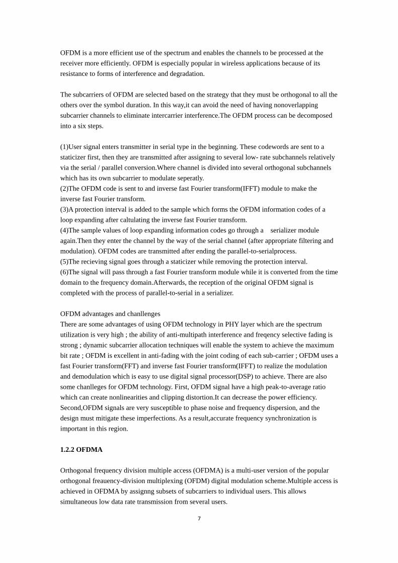
1.2.3 Antenna Techniques

The antenna technique is very important in any radio transmission. Nowadays, there are some

kinds of Multiple Anetenna Techniques such as SISO(single input single output), MISO(multiple

input single output), SIMO(single input multiple output), MIMO(multiple input multiple output).

The usage of multiple antenna techniques make a big breakthrough of improving the signal

robustness and increasing the system capacity as well as user data in the case of spatial diversity

of the radio channel. The figure of antenna techniques is presented below.

Multiple-input multiple-output (MIMO) techniques have been extensively adopted in the IEEE

802.16d/e/j standards to improve both the cell coverage and average user experience[1]

. Examples

of MIMO techniques include single-user MIMO (SU-MIMO), multiuser MIMO (MU-MIMO),

and cooperative relay. These new techniques allow flexible link configurations including both

point-to-multipoint and multipoint-to-point. For example, a base station (BS) employing spatial

division multiple access (SDMA) can send multiple data streams to multiple subscriber stations

(SSs) simultaneously on the same time-frequency resource, while multiple relay stations (RSs) can

cooperatively perform space-time coding to send data packets to one SS. However, each MIMO

technique is optimized for only a limited set of application scenarios. For example, transmit

beamforming requires channel station information at the transmitter (CSIT) and thus does not

perform well in high-mobility situations. The support of MIMO techniques also brings additional

equirements and constraints in system design and integration. Additional pilots for channel

training, for example, are required for the multiple transmit antennas in diversity modes. In

addition, the adoption of MIMO techniques often requires a tight design integration of PHY,

medium access control (MAC), and higher layers. Besides technical issues, cost plays an

important role for wider market penetration. Low-cost solutions such as antenna selection may be

appealing to certain markets.

10

Adaptive Antenna System is used in the WiMAX specification to describe beam-forming

techniques where an array of antennas is used at the BS to increase gain to the intended SS while

nulling out interference to and from other SSs and interference sources[2]

. AAS techniques can be

used to enable Spatial Division Multiple Access (SDMA), so multiple Sss that are separated in

space can receive and transmit on the same subchannel at the same time. By using beam forming,

the BS is able to direct the desired signal to the different SSs and can distinguish between the

signals of different SSs, even though they are operating on the same subchannel(s)

1.2.4 Physical Channelization

In WiMAX, the data to be transmitted is mapped to one or more logical sub-channels called slots

which is controlled by the scheduler. And the logical sub-channels are mapped to physical

subcarriers. The physical data and pilot subcarriers are uniquely assigned based on the type of

sub-channelization used. They are formed by two types of subcarrier allocations which are

distributed allocation and adjacent allocation. For distributed allocation , it pseudo-randomly

distributes the subcarriers over the available bandwidth thus providing frequency diversity in

frequency selective fading channels and inter-cell interference averaging. On the other hand, for

adjacent allocation, they are adjacent to each other in the frequency domain. Contiguous symbols

that use specific type of sub-channel assignment are called permutation zones. Here the zone types

used for sownlink and uplink are as follows.

Zone types Full names Functions

DL PUSC Downlink Partial Usage of

Sub-channels

Marking the start of all DL

frames following the preamble

and being maped into lager

groups.

UL PUSC Uplink Partial Usage of

Sub-channels

Four contiguous subcarriers

are grouped over three

symbols to form a tile.

DL FUSC Downlink Full Usage of

Sub-channels

Using all subcarriers to

provide a high degree of

frequency diversity.

DL OFUSC Downlink Optional FUSC A slight variation of FUSC

where pilot subcarriers are

evenly spaced by eight data

subcarriers.

UP OPUSC Uplink Optional PUSC Same as UL PUSC except

using a tile size

TUSC1 and TUSC2 Tile Usage of Sub-channels Simliar to DL PUSC and

OPUSC except using a

different equation for

assigning the subcarriers.

11

1.3 MAC layer in WiMAX

WIMAX MAC layer provides an interface betwwen the higher transport layers and the physical

layer. It takes MAC service data units (MSDUs) from upper layer and then organizes them into

MAC protocol data units(MPDUs) for transmission over the air. MAC layer does the reverse in

the receiving side.The greatest value of it is to provide for dynamic bandwidth allocation that

defeats the usual degradations of wireless services which are latency and jitter.

The WiMAX MAC layer is designed from the ground up to support very high peak bit rates while

delivering quality of service similar to that of ATM and DOCSIS. The WiMAX MAC layer uses a

variable-length MPDU and offers a lot of flexibility to allow for their efficient transmission. The

WiMAX MAC protocol is for point-to-multipoint broadband wireless access applicqtions while it

addresses the need for very high bit rates, both UL (to the BS) and DL (from the BS).The WiMAX

MAC accmmodeates both continuous and bursty traffic for the legacy TDM voice and data, IP

connectivity, and packetized VoIP require services of end users.Meanwhile, the WiMAX MAC

protocol supports a variety of backhaul requirements including both ATM and packet-based

protocols.

The WiMAX MAC layer includes three componentes which are the service-specific convergence

sublayer (CS), the common-part sublayer, and the security sublayer. The function of the CS is to

get data packets from the high layer while its location is between the MAC layer and layer 3 of the

network.The CS should perform all operations that are dependent on the nature of the higher-layer

protocol.It can be trained as a layer which can mask the higher-layer protocol and its requirements

from the rest of the WIMAX MAC and PHY layers. The common-part sublayer performs all the

packet operations that are independent of the higher layers.Obviously the security sublayer is to

make sure encryption, authorization, and proper exchange of encryption keys between the BS and

the SS.

1.4 Quality of Service in WiMAX

There are two broad definitions of Quality of Service(QoS)[3]

:

User-Centric QoS is the collective effect of service performances which determine the degree of

satisfaction of a user of the service.

Network-Centric QoS is the mechanisms that give network managers the ability to control the mix

of bandwidth, delay, variances in delay (jitter), and packet loss in the network in order to deliver a

network service (e.g., voice over IP). Here we focus on the second QoS which are

Network-Centric QoS.

Users insists on a transmission protocol that controls contention between themselves and enables

the service to be tailored to the delay and bandwidth requirements of each user application. This is

accomplished through four different types of UL scheduling mechanisms. These mechanisms are

implemented using unsolicited bandwidth grants, polling, and contention procedures. The

WiMAX MAC provides QoS differentiation[4]

for different types of applications that might

12

operate over WiMAX networks:

Unsolicited Grant Service : The Unsolicited Grant Service, UGS is used for real-time services

such as Voice over IP, VoIP of for applications where WiMAX is used to replace fixed lines such

as E1(E-carrier system) and T1(T-carrier).

Real-time Packet Services : This WiMAX QoS class is used for real-time services including video

streaming. It is also used for enterprise access services where guaranteed E1/T1 rates are needed

but with the possibility of higher bursts if network capacity is available. This WiMAX QoS class

offers a variable bit rate but with guaranteed minimums for data rate and delay.

Extended Real Time Packet Services : This WiMAX QoS class is referred to as the Enhanced Real

Time Variable Rate, or Extended Real Time Packet Services. This WiMAX QoS class is used for

applications where variable packet sizes are used - often where silence suppression is

implemented in VoIP. One typical system is Skype.

Non-real time Packet Services : This WiMAX QoS class is used for services where a guaranteed

bit rate is required but the latency is not critical. It might be used for various forms of file transfer.

Best Effort : This WiMAX QoS is that used for Internet services such as e-mail and browsing.

Data packets are carried as space becomes available. Delays may be incurred and jitter is not a

problem.

The scheduling reservation management details are not standardized even though extensive

bandwidth allocation and QoS mechanisms are provided . In fact, the standard supports scheduling

only for fixed-size real-time service flows. The scheduling of both variable-size real-time and

non-real-time connections is not considered in the standard. Thus, WiMAX QoS is still an open

field of research and development for both constructors and academic researchers. The standard

should also maintain connections for users and guarantee a certain level of QoS. Scheduling is the

key model in computer multiprocessing operating system. It is the way in which processes are

designed priorities in a queue. Scheduling algorithms provide mechanism for bandwidth allocation

and multiplexing at the packet level.

The bandwidth allocation requests are divided into specified class after going though the classifier

in subscriber stations.Then the allocation requests combine QoS Parameters are sent to subscriber

station scheduler and transmitted to base station considering the channel conditions. At base

station, the uplink scheduler decides which request should be accepted and which are going to be

abondoned based on uplink scheduling alogrithm. The information of it is included into Uplink

Map which is given back to the subscriber station. Afterwards, SSs starts to sending their data

based on it. With connction admission control and QoS parameters, the base station also make

decisions of the piriorities of the data which are transmitting back to subscriber stations. All the

request and frame are though physical layer. Here is the figure of overrall structure of the WiMAX

QoS architecture.

13

There are many scheduler proposals for WIMAX while most of them focus on the BS

scheduler,epecially Downlink-BS scheduler. Downlink-BS scheduler can get the information

about queue and packets easily. For Uplink-BS scheduler, the polling mechanism has to be

considered to guarantee the QoS. It is obvious that splitting the allocation bandwidth among the

connections is decided by BS scheduler when the QoS parameter can be assured.

Nowadays, the mainstream scheduling techniques for WiMAX can be divided into two catagories

which are channel-unaware schedulers and channel-aware schedulers. In details, channel-unaware

schedulers do not use the information of the channel conditions in makeing the scheduling

decision while generally assume error-free channel so that it is easier to reach the QoS assurance.

For channel-aware schedulers, it is important to consider the sigal attenuation, fading, inerference

and noise effect during the transmission process. It is more wise tfor scheduler designers to take

into account the channel condition in ouder to optimally and efficiently make the allocation

decision.

The schedulers for WiMAX can be classified into two categories which are intra-class scheduling

and inter-class scheduling. In details, intra-class scheduling is to allocatie the resource within the

same class given the QoS requiements. The main issue for inter-class schduling is whether each

traffic class should be considered separately, that is, have its own queue. The channel-unaware

scheulers and channel-aware schedulers are going to be presented below.

1.4.1 Channel-Unaware Schedulers

This type of schedulers makes no use of channel stat conditions such as the power level, channel

error and loss rates. These basically assure the QoS requirements among five classes-mainly the

delay and thoughput constraints[5]

. Some channel-unaware scheduling are introduced below.

Round Robin(RR) algorithm : Aside from FIFO, RR allocation can be considered the very first

14

simple scheduling algorithm. RR fairly assigns the allocation one by one to all connections. The

fairness considerations need to include whether allocation is for a given number of packets or a

given number of bytes. With packet based allocation, stations with larger packets have an unfair

advantage.

Earliest Deading First(EDF) algorithm : EDF belongs to Delay-based algorithms which are a set

of schemes is specifically designed for real-time traffic such as UGS,ertPS and rtPS service

classes, for which the delay bound is the primary QoS parameter and basically the packets with

unacceptable delays are discarded. EDF serves the connection based on the deadline.

Priority-based algorithm(PR) : In order to guarantee the QoS to different classes of service,

priority-based schemes can be used in a WiMAX scheduler. For example, the priority order can

be : UGS, ertPS, rtPS, nrtPS and BE, respectively.

These algorithm upon is either intra-class scheduling or inter-class scheduling in channel-unaware

catalogy. Moreover, some schduling designers invent some scheduling algorithms whicn can

combine both inter-class scheduling and intra-class schduling nowadays.

Two-Tier Scheduling Algorithm(2TSA)[6]

: 2TSA is implemented only at BSs. The objectives are

to achieve both QoS guarantee and fairness. The first-tier and second-tier scheduling is

category-based and weight-based, respectively. 2TSA first allocates bandwidth to the “unsatisfied”

category. While still being with more available bandwidth, it then allocates bandwidth to

connections belonging to “satisfied” category, and followed by “over-satisfied” category.

Therefore, the first-tier bandwidth allocation is to ensure that each connection can be satisfied

with their minimum requirement. Then for a specific category, the received bandwidth is further

distributed to connections based on the parameter of weight. The smaller weight of a connection,

the higher bandwidth allocation priority it has. After finishing this two-tier bandwidth allocation,

the BS generates the corresponding UL-MAP and broadcasts to all.

1.4.2 Channel-Aware Schedulers

The channel-aware schedulers can be classified into four classes based on the primary objective :

fairness, QoS guarantee, system thoughput maximization and power optimization[11]

. Basically,

the BS downlink scheduler can use the Carrier to Interence and Noise Ratio(CINR) which is

reported back from the SS via the Channel Quality Indicator(CQI) channel. For uplink scheduling,

the CINR is measured directly on previous transmissions from the same subscriber station. Most

of the purposed algorithms have the common asumption that the channel condition does not

change within the frame period. Also, it is assumed that the channel information is known at both

the transmitter and the receiver.

1.Fairness : This metric mainly applies for the Best Effort(BE) service. One of the commonly used

baseline shcdulers in published rersearch is the Proportional Fairness Scheme(PFS). The objective

of PFS is to maximize the long-term fairness.

15

2.QoS Guarantee : Modified Largest Weighted Delay First (MLWDF) can provide delays smaller

than a predefiend threshold value with a given probability for each user(rtPS and nrtPS). And, it is

provable that the throughput is optimal for LWDF. The algorithm can achieve the optimal

whenever there is a feasible set of minimal rates area. The algorithm explicityly uses both current

channel condition and the state of the queue into account.

3.System Throughput Maximization : Some schemes are focus on maximizing the total system

thoughput. A maximum system throughput approach is the exponential rule in that it is possible to

allocate the minimum number of slots derived from the minimum modulation scheme to each

connection and then adjust the weight according to the exponnet(p) of the instant modulation

scheme over the minimum modulation scheme. This scheme obviously favors the connections

with better modulation scheme(higher p). Users with better channel conditions receive

exponentially higher bandwidth. Two issues with this scheme are that additional mechanisms are

required if the total slots are less than the total minimum. And, under perfect channel conditions,

connections with zero minimum bandwidth can gain higher bandwidth than those with non-zero

minimum bandwidth.

4.Power Constraint : The purpose of this class of algorithms is not only to optimize the throughput

but also to meet the power constraint. In general, the transmitted power at a subscriber station is

limitted. As a result, the maximum power allowable is introduced as one of the constraints. Lest

amount of transmission power is perferred for mobile users due to their limitted battery capacities

and also to reduce the radio interference. Link-Adaptive Large-Weighted-Throughput(LWT)

algorithm has been proposed for OFDM systems. LWT takes the power consumption into

consideration. The suboptimal Hungarian of Liner Programming algorithm with adaptive

modulation is used to find the subcarriers for each user and then the rate fo the user is iteratively

incremented by a bit loading algorithm, which assigns one bit at a time with a greedy approach to

the subcarrier. Since this suboptimal and iterative solution is greedy in nature, the user with worse

channel condition will mostly suffer.

Some detailed algorithms of channel-aware are presented below.

TCP-Aware Uplink Scheduling Algorithm[7]

: This algorithm works with only one class of 4

classes defined for QoS. It deals with BE class. As this class has not any specific QoS requirement

it is not advantageous to use bandwidth request mechanism for this class and to waste that

bandwidth. Also, it is not advisable to equally allocate remaining bandwidth to all remaining BE

connections because all connections can’t utilize all bandwidth allocate to them and some may

have more requirements than allocated. So, this algorithm works by calculating bandwidth for a

particular connection according to sending rate of that connection. Also as sending rate is going to

change dynamically, it is not proper to allocate fix amount of bandwidth to a particular

connection.

Hierarchical Channel-Aware Uplink Algorithm[8]

: This scheduling rule is a hierarchical channel

aware scheduling algorithm for uplink scenario. Weights of the service classes are adaptive

according to the QoS requirements of each service class. Weights of the subscriber stations are

16

assigned based on their channel quality and bandwidth requests. This algorithm leads to improving

overall system throughput without starving lower priority service class.

Intra-Class Channel-Aware Scheduling Algorithm[9]

: This proposed algorithm uses battery level as

a new parameter to determine the weights. It is designed for nrtPS class and belongs to intra class

scheduling method. First, the number of subcarriers to be assigned to each other is determined.

Afterwards, assign the remaining subcarriers to the users. After calculate the number of

subcarriers per each user and user’s priority, the author introduced a new priority metric to

subcarrier allocation. As a result, according to this metric, users with higher arrival rate in

previous frame, lower battery level and long-term throughput has the priority to get service.

2. LTE technology

2.1 Introduction of LTE

LTE, an initialism of long-term evolution, marketed as 4G LTE, is a standard for wireless

communication of high-speed data for mobile phones and data terminals. It is based on the

GSM/EDGE and UMTS/HSPA network technologies. It is aiming for maximum 100 Mbps

downlink and 50 Mbps uplink speed when using 20 MHz bandwidth so that it can enable diverse

mobile multimedia service provision. The standard is developed by the 3GPP which is 3rd

Generation Partnership Project.

The basic protocol structure of LTE is made by radio link control(RLC) and medium access

control (MAC) layers which are responsible for retransmission handling and multiplexing of data

flows. The duty of physical layer is to transmit and modulate the data. The structure of LTE

protocol is presented below[10]

.

17

2.2 PHY layer in LTE

2.2.1 OFDMA and SC-FDMA

LTE systems decides to use OFDMA in its downlike side. However , the situation in its uplink

side is kind of different. The fact is that the available transmission power is much lower than it in

download side. The highly power-efficient transmission should be considered in the uplink design

as well. One single-carrier transmission, based on discrete Fourier transform (DFT)-precod- ed

OFDM, sometimes also referred to as single-carrier frequency-division multiple access

(SC-FDMA), is used for the LTE uplink.

SC-FDMA[11]

deals with the assignment of multiple users to a shared communication resource as

other multiple access schemes. SC-FDMA can be interpreted as a linearly precoded OFDMA

scheme, in the sense that it has an additional DFT processing preceding the conventional OFDMA

processing. The process transmission of SC-FDMA scheme is very similar to OFDMA. For each

user the sequence of bits transmitted is mapped in a complex constellation symbols (BPSK, QPSK

or M-QAM). This different transmitters (users) are assigned different Fourier coefficients. This

assignment is carried out in the mapping and demapping blocks. The receiver side includes one

demapping block, one IDFT block and one detection block for each user signal to be received. Just

like in OFDM , guard intervals with cyclic repetition are introduced between blocks of symbols in

view to efficiently eliminate time spreading (caused by multi-path propagation) among the blocks.

In SC-FDMA, multiple access among users is made possible by assigning different users, different

sets of non-overlapping fourier-coefficients (sub-carriers). This is achieved at the transmitter by

inserting (prior to IFFT) silent fourier-coefficients (at positions assigned to other users), and

removing them on the receiver side after the FFT.

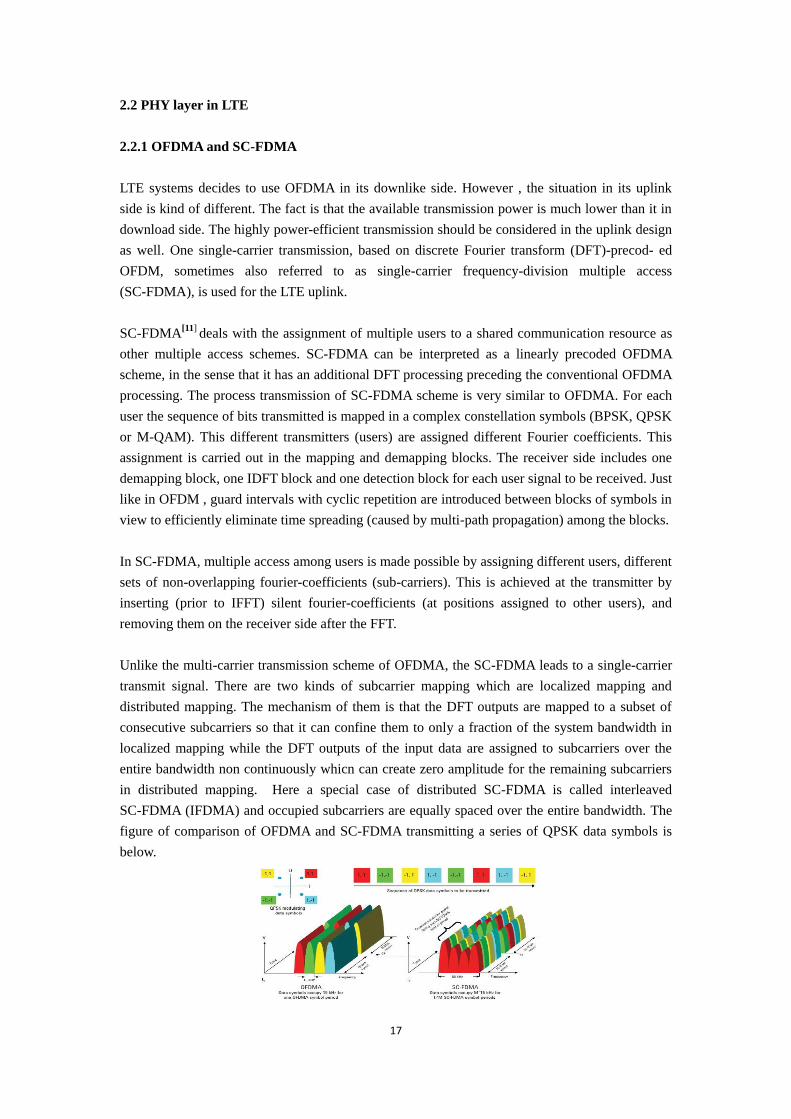
Unlike the multi-carrier transmission scheme of OFDMA, the SC-FDMA leads to a single-carrier

transmit signal. There are two kinds of subcarrier mapping which are localized mapping and

distributed mapping. The mechanism of them is that the DFT outputs are mapped to a subset of

consecutive subcarriers so that it can confine them to only a fraction of the system bandwidth in

localized mapping while the DFT outputs of the input data are assigned to subcarriers over the

entire bandwidth non continuously whicn can create zero amplitude for the remaining subcarriers

in distributed mapping. Here a special case of distributed SC-FDMA is called interleaved

SC-FDMA (IFDMA) and occupied subcarriers are equally spaced over the entire bandwidth. The

figure of comparison of OFDMA and SC-FDMA transmitting a series of QPSK data symbols is

below.

18

The bigges advantage of SC-FDMA comparing to OFDM is that it can provide robust resistance to

multipath without the big problem of high PAR (peak-to-average ratio) which is caused by OFDM

technology when the number of subcarriers increase.Although the performance gap is not much.

At the same time, frequency-selevtive fading and phase distortion can be combated since

equalization is achieved on the receiver side after the FFT calculation by multiplying each Fourier

coefficient by a complex number.

2.2.2 Multiple Antenna Techniques

Three multiple antenna schemes can be uesd which are Tx diversity(MISO), Rx diversity(SIMO),

Spatial Multiplexing (MIMO) for LTE downlink side.

For Tx diversity , it surpports open-loop configuration other than closed-loop Tx diversity which

is more complicated. For Rx diversity, it is mandatory for LTE User Equipment (UE) while

making of the baseline receiver capability. The SNR(Signal-to-Noise-Ratio) is improved by

maximum ratio combining of received streams. For Spatial Multiplexing (MIMO), LTE uses the

two or four antenna configurations. A two channel UE receiver allows 2x2 or 4x2 MIMO,

common being the 2x2 Single-User MIMO(SU-MIMO) for LTE. In SU-MIMO, the payload data

is made by two code word streams while each code word is represented at different powers and

phases on both antennas. Here the closed-loop form of MIMO with pre-coding of streams that

channel information can be aquired on the uplink control channed of the UE is used.

For LTE uplink side, battery power and cost must be considered for the LTE User Equipment(UE).

MU-MIMO(Multiple-User Multiple Input Multiple Output) where two different UE transmit in

the same frequency and time to the eNB is used here. This configuration has the advantage to

obtain double the uplink capacity without extra costs to UE. In addition, a second transmit antenna

can be allowed to use uplink Tx diversity and SU-MIMO to enable higher data rates depending on

channel conditions by the UE. For the eNB, Rx diversity is the baseline capability and LTE

supports two or four receive antennas.

2.2.3 Physical Channelization

The physical signals are generated in the Layer 1 and used for system synchronization, cell

identification and radio channel estimation. Meanwhile, the function of physical channels is to

provide a means of carrying data from higher layers which are control, scheduling and user

payload. The details of them are presented below.

DL Signals Full name Function

P-SCH Primary Synchronization signal Cell search and identification by

UE.Carries part of cell ID.

S-SCH Secondary Synchronization signal Cell search and identification by

UE.Carries remainder of cell ID.

RS Reference Signal(Pilot) DL channel estimation.Exact

19

sequence derived from cell ID.

UL Signals Full name Function

RS Reference Signal(Demodulation and

sounding)

Used for synchronization to the UE

and UL channel estimation.

DL Channels Full name Function

PBCH Physical broadcast channel Carries cell-specific information

PMCH Physical multicast chqnnel Carries the MCH transport channel

PDCCH Physical downlink control channel Scheduling, ACK/NACK

PCFICH Physical control format indicator

channel

Defines number of PDCCH

OFDMA symbols per

sub-frame(1,2,or 3)

PDSCH Physical downlink shared channel Payload

PHICH Physical hybrid ARQ indicator

channel

Carries HARQ ACK/NACK

UL Channels Full name Function

PRACH Physical random access channel Call setup

PUCCH Physical uplink control channel Scheduling,ACK/NACK

PUSCH Physical uplink shared channel Payload

2.3 MAC Layer in LTE

The main funcions of MAC Layer in LTE are mapping between transparent and logical channels,

error correction through hybrid ARQ, priority handling with dynamic scheduling and logical

channel prioritization.

MAC layer of LTE divided into two planes : user plane and control plane. User planes includes

Packet Data Convergence Protocol sublayer(PDCP), Radio Link Control sublayer(RLC) and

MAC sublayer. Their functions are data header compression, encryption, Automatic Repeat

Request(ARQ) and Hybrid ARQ(HARQ). Control plane contains Radio Resource Control

sublayer(RRC), PDCP sublayer, RLC sublayer and MAC sublayer. PDCP sublayer offers the

protection of encryption and integrity. The function of RLC and MAC layers are the same as they

are in the user plane. RRC sublayer provides broadcasting, paging, RLC connection management,

radio bearer control, mobility, UE measurement reporting and control functions. Normally, PDCP

sublayer, RLC sublayer and MAC sublayer are call L2 layer in LTE.

Radio Resource Control(RRC)

20

RRC is the key component in radio resource management of E-UTRAN. The main functions of

RRC are broadcasting system information, paging, establishment, maintenance and release the

RRC connection between terminal and E-UTRAN; security and key management; establishment,

maintenance and release point-to-point radio bearer; mobility management including measurement

control, reporting, switching, cell selection and reselection and RRC context switching

transmission; broadcasting MBMS service; establishment, maintenance and release of MBMS

radio bearer; QoS management; terminal measurement control and reporting; operating parameter

configuration of the underlying layer.

Packet Data Convergence Protocol(PDCP)

PDCP provides the compression of IP data header, encryption and integrity protection of

transforming data. The IP data header mechanism is based on Robust Header Compression(ROHC)

technique. At the receieving side, PDCP is responsible for the decryption and decompression

operation. For mobility terminal, each radio bearer configures a PDCP entity.

Radio Link Control(RLC)

RLC is responsible for segmentation / restructuring, retransmission processing and sequential

transmission. RLC provide services to PDCP by the way of radio bearer. Each raido bearer has

only one RLC entity.

MAC

MAC is to deal with HARQ, uplink and downlink scheduling. For uplink and downlink, each cell

only has one MAC entity. There are HARQ parts in both sending and receiveing sides of MAC.

MAC offers service to RLC layer by logical way.

2.4 Quality of Service in LTE

The QoS level of granularity in the LTE evolved packet system (EPS) is bearer wich is a packet

flow established between the packet data network gateway(PDN-GW) and the user terminal. The

traffic running between a particular client application and a service can be differentiated into

separate service data flows(SDFs). Here SDFs mapped to the same bearer will get a common QoS

treatment. A bearer is assigned a scalar value referred to as a QoS class identifier (QCI) which

specifies the class to which the bearer belongs. QCI refers to a set fo packet forwarding treatments

preconfigured by operator for eqch network element. The class-based method improves the

scalability of the LTE QoS framework.

There are two types of bearers[12]

:

Guaranteed bit rate (GBR): Dedicated network resources related to a GBR value associated with

the bearer are permanetly allocated when a bearer becomes established or modified.

21

Non-guaranteed bit rate (non-GBR): A serveice utilizing a non-GBR bearer may experience

congestion-related packet loss.

GBR bearers are provisioned in the sense that their bandwidth requirements are checked against

the current cell utilisation before alooing or disallowing the connection to be formed. Non-GBR

bearers have no guaranteed allocation of resources and hence provide a best-effort service.

2.4.1. Scheduling

For Uplink MAC Scheduling, it determimes which berares get how much of the allocation at the

UE, essentially within-UE scheduling. It works on grants received from the eNB. Here MAC tells

RLC to sent Xi bits from logical channel i while scheduler is based on Bearer's QoS requirements.

For Downlink Scheduling at the eNB, it is significantly more complex than at UEs. eNB controls

channel usage in both UL and DL. There are some factors affecting shceduling which are: Traffic

volume for each bearer at each UE and it schedules Ues with beareres having backlog, QoS

Requirements of each bearer at each UE, Radio conditions at UEs which are identified through

measurements made at the eNB and reported by the UE.

LTE systems use multi-user scheduling for it changes in the range of distributing available

resources among active users so that QoS needs can be achieved.

The portions of the spectrum should be distributed each TTI(transmission time interval) among

them since the data channel is shared among the users. The scheduler performs the allocation

decision valid for the next TTI and sends such information to UEs while using the PDCCH for

each TTI. OFDMA can provide no inter-channel interference so that schedulers of eNB can be

deployed. They work with a granularity of one TTI and one RB(resource block) in the time and

frequency domain, respectively.

There are some attributes to be concidered when the allocation strategies designed which are

complexity and scalability, spectral efficiency, faireness and QoS provisioning. Meanwhile,

several aspects of LTE deployment in real environment may have effect on the decision to make

the best allocation strategies as uplink limitations, control overhead, limitations on the multi-user

diversity gain, energy consumption.

Four groups of strategies are made for the alloction of LTE which differ in theams of input

parameters, ojectives and service targets.

2.4.2. Channel-unaware schedulers

Based on the assumption of time-inveariant and error-free transmission media. There are some

channel-unaware algrithoms such as First In First Out Algorithm, Round Robin Algorithm, Blind

22

Equal Throughput Algorithm and Weighted Fair Queuning Algorithm.

2.4.3. Channed-aware schedulers

Channel State Information (CSI) feedbacks can be periodically sent from UEs to eNB by using ad

hoc control messages. The scheduler can estimate the channel quality perceived by each UE. QoS

differentiation is handled by associating a set of QoS parameters to each flow. The scheduler can

deal with data to guarantee some minimum required performances in the case of knowing the

values of such parameters. The maximum achievable throughput can be predicted as a result. First

Maximum Expansion which is to assing resources starting from the highest metric values and

“expanding” the allocation on both sides of M. Each UE is considered served whenever another

UE having better metrice is found.

2.4.4. Semi-persistent Scheduling for VoIP support schedulers

Semi-persistent allocation aims at increasing the VoIP capacity of the network in terms of

maximum number of contrmporary supported VoIP calls. They are not specifically conceived for

improving spectral efficiency or for reducing packet delay. They can be considered in practice as

channel-unaware approaches.

2.4.5. Energy-aware schedulers

Energy saving solutions can be applied to both eNB and UE. For what concern end-user devices,

power consumption can be limited through DRX procedures and the persisten allocation,which is

at the present the only allocation strategy able to meet this goal.

Some detailed algorithms of LTE are presented as follows.

Adaptive Transmission Bandwidth (ATB) PS algorithm[13]

: The main motivation for integrating

the ATB into the PS functionality is not only the simplification of the RRM functionalities but

mostly the need of providing a more flexible algorithm which can accommodate for different

traffic types - e.g. VOIP, which requires a limited bandwidth - as well as UEs with different power

capabilities. The advantage of this approach is that no additional functionality is required to tune

the bandwidth, that is, the capability of coping with varying traffic loads and power limitations is

inbuilt in the algorithm .

Time Domain Packet Scheduling (TDPS) algorithm[14]

: This GBR-aware packet scheduler is used

in TD, which prioritize the users according to the metric in MTD,i = GBRi/Ri giving highest

priority to the user which is farthest below its GBR requirement. Ri is the past average throughput

of user i calculated using exponential average filtering.

MAC Scheduling Scheme for VoIP Traffic Service alogorithm[15]

: The key ideas of this scheme

are a VoIP priority mode and its adaptive duration management. Since the VoIP priority mode

assigns PRBs first to VoIP calls, it is able to minimize VoIP packet delay and loss, but the adaptive

23

duration management is able to prevent the overall system performance degradation, which is a

possible negative effect of the VoIP priority mode. In our scheme, the duration of VoIP priority

mode is dynamically adjusted according to VoIP packet drop rates. As a result, we are able to

achieve both the QoS satisfaction and the minimization of the negative effect.

Reference AC algorithm[16]

: The reference AC algorithm decides to admit a new user if the sum of

the GBR of the new and the existing users is less than or equal to a predefined Rmax as expressed

in ∑ 𝐺𝐵𝑅𝑖𝐾𝑖=1 +GBRnew ≤ Rmax, where K is the number of existing users in the cell. The users in a

cell require different amount of resources to fulfil their required GBR as it depends on their radio

channel quality. A drawback of the reference AC algorithm is that it treats all the users equally and

does not differentiate them based on their channel quality. Furthermore, Rmax is a tunable

parameter and does not represent the actual average uplink cell throughput, which is time-variant

as it depends on the resources allocated to the users and their experienced channel quality.

3.Comparision between WiMAX and LTE

3.1 Architecture

WiMAX

The basic requirements of WiMAX are supports for both fixed and mobile access deployments,

unbundling of access, connectivity, and application services to allow access infrastructure sharing

and muliple access infrastructure aggregation. The goal of the WiMAX design is to meet theses

requirements with getting the biggest the use of open standards and IETF protocols in a simple

all-IP architecture[17]

.

A network reference model(NRM) can explain the baseline WiMAX network architecture.

WiMAX uses the technique of both network access providers(NAPs) and network service

providers(NSPs). NAP provides WiMAX radio access infrastructure. Meanwhile, NSP surpports

IP connectivity and services to WiMAX subscribers basing some negotiated service level

agreements(SLAs). One NSP can have a relationship with multiple NAPs in one or differrent

geographical locations wihin this network architecture. The WiMAX NRM has serveral logical

network entities as components such as Subscriber Stations(SSs), an access service network(CSN),

a connectivity service network(CSN), their interactions through reference points R1-R8. Here

each SS, ASN and CSN possess some functions which are presented below.

Subscriber Station(SS) refers to a generalized equipment set providing connectivity between

subscriber equipment and a Base Station in the mobile wireless network.

Access Service Network(ASN) performs various network functions which can provide radio

access to the SS. The functions are Layer 2 connectivity to the SS ; Messages transmission of

Authentication, Authorization and Accounting(AAA) to the H-NSP(Home NSP) ; Preferred NSP

discovery and selection ; Relay functionality for establishing Layer 3 connectivity with SS ; Radio

ressource management ; Surport ASN and CSN anchored mobility, paging and location

24

management as well as ASN-CSN tunneling

The ASN can be implemented as an integrated ASN where all functions are cloolcated in the same

logical entity or it may have a decomposed configuration in which the ASN functions are

selectively mapped into two separate nodes as a BS and an ASN getway(ASN-GW). A

decomposed ASN may have one or more BSs with at least one instance of an ASN-GW.

Base Station(BS) is a logical network entity that primarily performs the radio related functions of

an ASN interface with the SS. Each BS is associated with one sector with one frequency

assignment but may incorporate additional DL and UL scheduler.

ASN gateway(ASN-GW) represents an aggregation of centralized funcions related to QoS,

security, and mobility management for all the data connections as a logical entity.Meanwhile, it

can host functions related to IP layer interactions or with other ASN.

BS and ASN-GW can have ont to many or many to one relationship which can surpport loading

balancing and redundancy options.

Connectivity service network(CSN) provides IP connectivity services to WiMAX subscribers and

comprises of network elements such as routers, AAA proxy/servers, home agent, user databases

and interworking gateways or enhanced network servers to support multicast, broadcast and

location based services. CSN has some functions which are IP address management, AAA proxy

or server ; QoS policy cand admission control based on user subscription profiles ; ASN-CSN

tunneling support ; Subscriber billing and interoperator settlement ; Inter-CSN tunneling for

roaming ; CSN-anchored inter-ASN mobility ; Connectivity to Internet and managed WIMAX

services such as IP multimedia services(IMS), location-based services, peer-to-peer services, and

broadcast and multicast services ; Over-the-air cativation and provisioning

The WiMAX NRM is illustrated as follows[17]

.

25

LTE

The logical baseline architecture for 3G is complicated today and the figure of it is decribed below.

3GPP's goal is to simplify the 3G architecture and define an all-IP, packet-only core network wich

is evolved packet core(EPC). LTE has to implement EPC to meet some goals of it[18]

.

The aimes of LTE architecture are to provide open interfaces to support multi-vendor deployments

and robustness-no single point of failure, support multi-Radio Access Technology(RAT) with

ressources controlled from the network and seamless mobility as well as maintain appropriate

level of security.To acquire these goals, LTE model decides not to use Radio Network

Controller(RNC). The LTE has evolved the EPC interact with legacy radio access technologies as

follows.

26

The architecture of the LTE RAN is also simplified as the EPC. The figure following presents the

E-UTRA which includes a new network element, the eNB providing the E-UTRA user plane and

control plane protocol terminations toward the user equipment (UE).

From the figure, a new interface called X2 connects the eNBs as a mesh network which

communicates directly between the elements and liminating the need to funnel data back and forth

through a RNC. The E-UTRAN is connected to the EPC via the S1 interface while connecting the

eNBs to the mobility management entity(MME) and serving gateway(S-GW) elements through a

'many-to-many' relationship.

This new architecture pushes more siglaling down to the eNBs by splitting the user plane and

mobility management entities as depicted in the figure below[19]

.

The eNB has some functions such as radio ressource management, IP header compression and

encryption, selection of MME at UE attachment, routing of user plane data towards S-GW,

27

scheduling and transmission of paging messages and broadcast information, measurment and

measurement reporting configuration for mobility and scheduling, scheduling and transmission of

ETWS messages.

The MME has many functions including non-access stratum(NAS) signaling and NAS signaling

security, access stratum(AS) security control, idle state mobility handling and EPS bearer control

The S-GW hosts these function which are mobility anchor point for inter eNB handovers,

termination of user-plane packets for paging reasons and switching of user plane for UE mobility.

The packet data network(PDN) gateway(P-GW) provides such functions as UE IP address

allocation, per-user-based packet filtering and lawful interception.

3.2 Frame structure

WiMAX

For WiMAX, a frame duration of 5 ms is used along with time division duplexing(TDD)[20]

. To

allocate for DL and the rest of UL transmissions, the fame is splitted into OFDM symbols. The

first symbol in the frame is used for preamble transmission which is used by the SS for BS

identification, timing synchronization and channel estimation. Subchannels are formed out of a

group of subcarriers and used to send control and data transmissions. A typical allocation spans the

subchannel and symbol axes and typically a 2-dimensional region is assigned for a transmission

for both DL and UL transmissions. The base station(BS) announces a schedule each frame period

to vonvey the DL and UL allocation. To avoid interferenc between downlink and uplink signals,

they are separated by small time gaps called Transmit Time Gap(TTG) for the transition from

downlink sub-frame to uplik sub-frame and Receive Time Gap(RTG) for the transition from

uplink sub-frame to downlink sub-frame.

LTE

LTE uses two frame structure: frame structure type 1(FS1) for full duplex and half duplex FDD,

frame structure type 2(FS2) for TDD.

For FS1, the frame duration of 10 ms is divided into subframes of 1 ms duration. Each subframe is

consist of two slots of 0.5 ms duration. The FS1 is identical in the uplink and downlink in terms of

frame, sub-frame, and slot duration however the allocation in terms of physical signals and

channels is different. The uplink and downlikn transmissions are separated in the frequency

domain.

For FS2, it is made of two 5 ms half-frames for a total duration of 10 ms for a 5 ms switch-point

periodicity. Su-frames consists of a uplink or a downlink transmission besides some subframes

have uplink and downlink at the same time which are separated by a transmission gap(GP).

Allocation procedure is decided by one of the seven differrent configurations. Here, subframes 0

28

and 5 are for downlink frame while sub-frame 1 is for a both-links frame. The composition of

other sub-frames varies based on the configuration.

3.3 MIMO technology

WiMAX

In the region of open-loop transmit diversity, Space-frequency block coding(SFBC) with precoder

cycling is used while single codeword with precodercycling is supported in the region of

open-loop spatial multiplexing. For closed-loop spatial multiplexing, WiMAX uses advanced

beamforming and precoding. In multi-user MIMO side, closed-loop and open-loop MU-MIMO

are allowed. At downlink side, WiMAX can meet the requirement of up to 8 streams with

SU-MIMO while up to 4 users(non-unitary precoding) with MU-MIMO. The data will change into

up to 4 streams with SU-MIMO and up to 4 users with MU-MIMO at uplink side.

LTE

For LTE, it uses SFBC or SFBC with frequency-switched transmit diversity(FSTD) in open-loop

transmit diversity technique while multiple codewords with large delay clclic delay diversity(CDD)

is employed in open-loop spatial multiplexing. For closed-loop spatial multiplexing, LTE allows

codebook-based precoding and UE-specific RS based beamforming.Meanwhile, closed-loop

MU-MIMO is used in multi-user MIMO. LTE can allow up to 4 streams with SU-MIMO and up

to 2 users(unitary precoding) with MU-MIMO at downlink side. For uplink side, 1 stream with

SU-MIMO and up to 8 users with MU-MIMO can be supported.

3.4 MAC Layer

WiMAX

Control Plane

MAC layer of WiMAX is connection-oriented. Communication between SS and BS is controlled

by the MAC controlling messages including network access, distance measurement, swiching, idle

/ sleep modes processes which need the interaction between and SS and BS. The functions of

control plane and data plane in MAC are implemented in MAC CPS sublayer. For control plane,

the main functions are connection management, network access, bandwidth allocation, service

QoS, radio bearer control, switching control, multicast and broadcast.

Data Plane

MAC data plane of WiMAX has differrent functions at sending and receiving sides. For sending

side, the data are packaging into appropriate MAC PDU based on specific bandwidth allocation

with reading amount of Protocal Data Unit(PDU) and combining service flow tranforming

strategies. In the process of packaging, many mechanism such as fragment and pack can be used

29

in the case of implementing by protocol strictly. For receiving side, CPS decompose MAC PDU

received from physical layer into MAC SDU based on standard MAC PDU format and also

combined ervice flow tranforming strategies first. Then CPS identificates CS PDU and MAC

management signaling correctly, and forward them to appropriate signaling MAC CS or

appropriate signaling receiver module. WiMAX also allows ARQ function which is mostly

acheived in the CPS data plane.

LTE

Control Plane

The function modules of LTE control plane are mostly in the RLC sublayer which are system

messages broadcasting, radio paging, RLC connection management, radio bearer control, mobility

management, QoS management, UE measurement reporting and controling, MBMS service

broadcasting and security management.

Data Plane

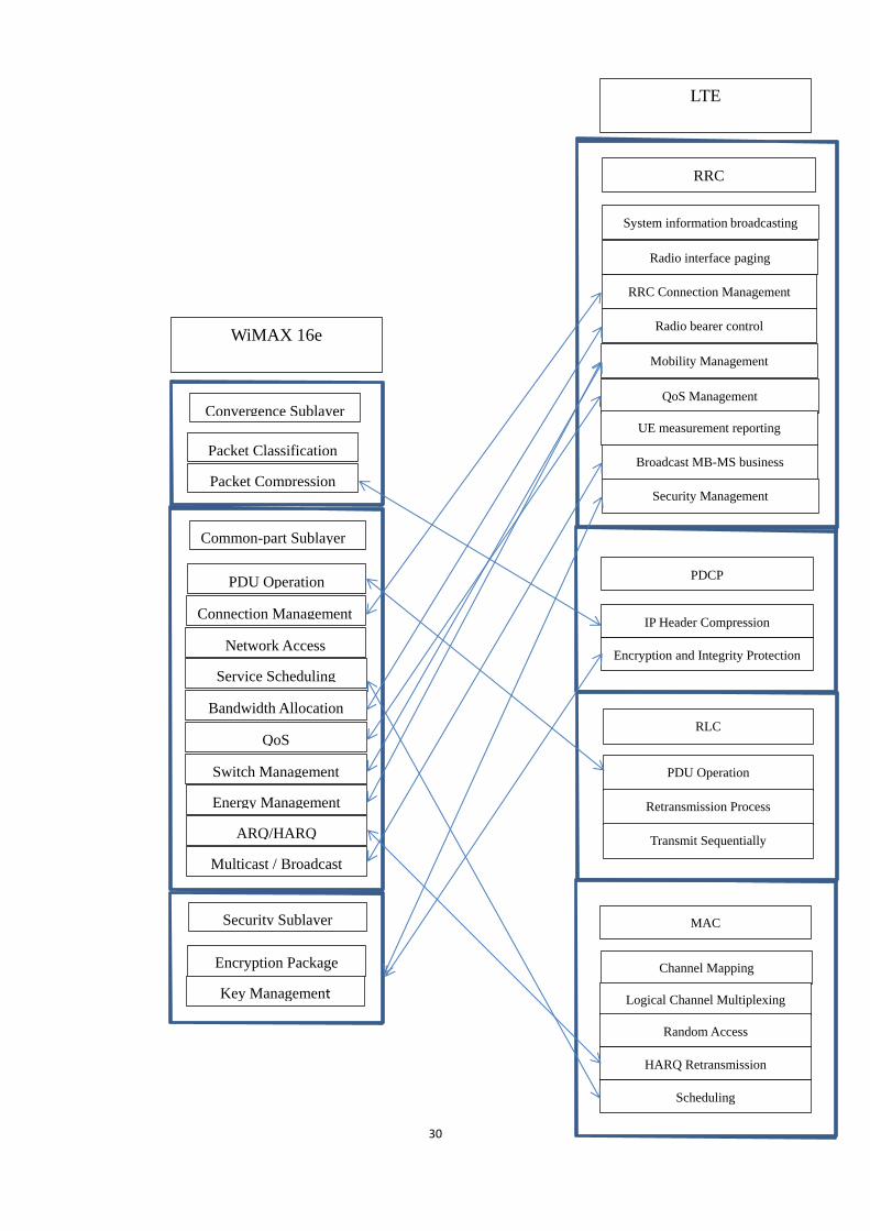
Data plane of LTE MAC layer is called user plane which contains the functions of PDCP sublayer,

RLC sublayer, MAC sublayer. The function module of PDCP sublayer mostly includes IP header

compression, encryption and integrity protection. RLC sublayer provides the PDU operation,

retransmission and sequential transmission. The functions of MAC sublayer are channel mapping,

logical channel multiplexing, random access, HARQ retransmission, uplink and downlink

scheduling. MAC sublayer offers service to RLC sublayer by logical channel which is defined by

the type of its bearer information.

The graph of the function module comparison for WiMAX and LTE is below

30

Convergence Sublayer

Packet Classification

Packet Compression

Common-part Sublayer

PDU Operation

Connection Management

Network Access

Service Scheduling

Bandwidth Allocation

QoS

Switch Management

Energy Management

ARQ/HARQ

Multicast / Broadcast

Security Sublayer

Encryption Package

Key Management

RRC

System information broadcasting

Radio interface paging

RRC Connection Management

Radio bearer control

Mobility Management

QoS Management

UE measurement reporting

Broadcast MB-MS business

Security Management

PDCP

IP Header Compression

Encryption and Integrity Protection

RLC

PDU Operation

Retransmission Process

Transmit Sequentially

MAC

Channel Mapping

Logical Channel Multiplexing

Random Access

HARQ Retransmission

Scheduling

WiMAX 16e

LTE

31

3.5 Multiple Access Technology

WiMAX uses OFDM and OFDMA techniques in both uplink and downlink sides. But there is a

big problem which is they will lead to a high Peak-to-average ratio(PAR). To avoid this problem

and also consider the power efficiency for user equipment, LTE decides to use SC-FDMA for its

uplink side and OFDMA for its downlink side.

3.6 QoS

Both WiMAX and LTE define a end-to-end IP based QOS but requires QoS requests to traverse

different protocol layers and differrent network portions. However, they define different attributes

and QoS types.

WiMAX

The key SF QoS attributes defined by WiMAX are as follows.

Attributes Full name Functions

MSTR Maximum sustained traffic rate Capping rate level of an SF

MTB Maximum traffic burst Maximum continuous burst a system

should accommodate for a service

ML Maximum latency Specifies maximum packet delay over the

air interface

TJ Tolerated jitter Specifies maximum packet delay

variation(jitter) for an SF

TP Traffic priority Priority of packets of different SFs based

on a combination of subscribers' profiles

and services mapped to SFs

UGI Unsolicited grant interval Time interval between successive data

grant opportunities for an SF over DL

UPI Unsolicited polling interval Maximal interval between successive

polling grant opportunitites for an SF over

UL

WiMAX define five classes of services which are presented below.

Classes Description Application

Unsolicited Grant Service(UGS) For Constant Bit Rate(CBR) and

delay-dependent applications

VOIP

Real-Time Polling Service(rtPS) For Variable Rate and delay dependent Streaming audio, Streaming video

32

application

Extended Real-Time Polling

Service(ertPS)

For variable Rate and delay dependent

applications

VOIP with silence suppression

Non-real-time Polling Service(nrtPS) Variable rate and non-real time application FTP

Best Effort(BE) Best Effort E-mail, web traffic

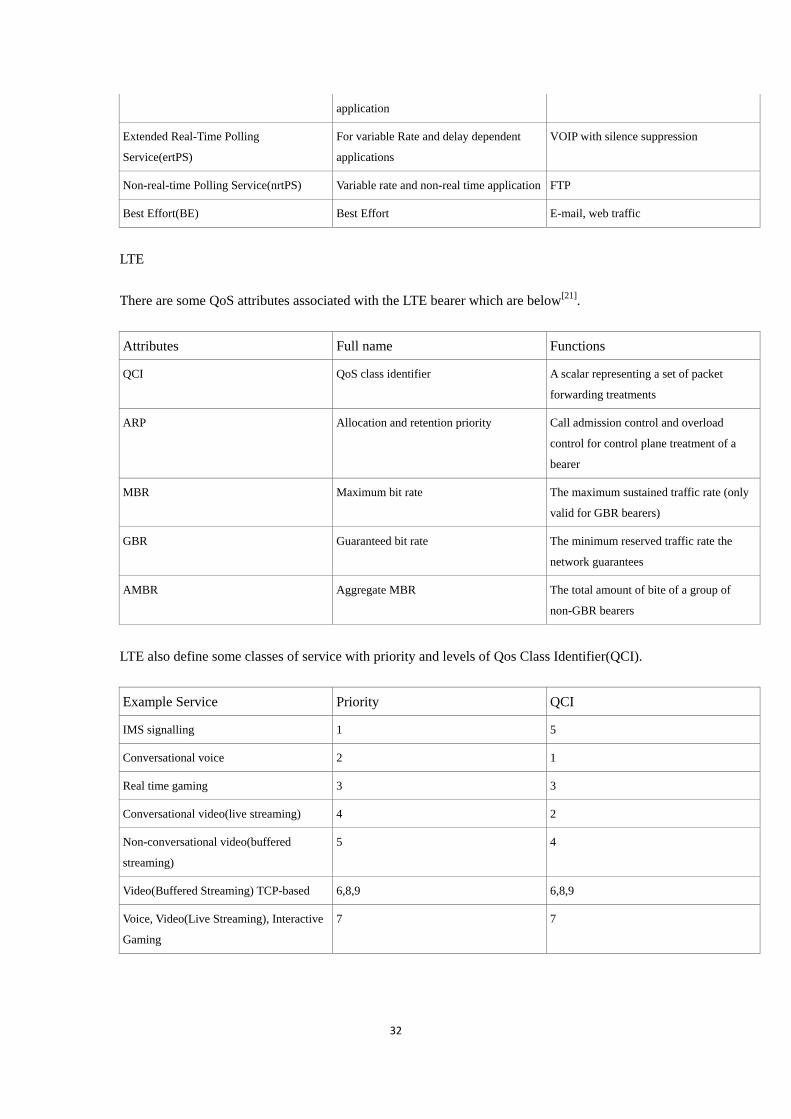
LTE

There are some QoS attributes associated with the LTE bearer which are below[21]

.

Attributes Full name Functions

QCI QoS class identifier A scalar representing a set of packet

forwarding treatments

ARP Allocation and retention priority Call admission control and overload

control for control plane treatment of a

bearer

MBR Maximum bit rate The maximum sustained traffic rate (only

valid for GBR bearers)

GBR Guaranteed bit rate The minimum reserved traffic rate the

network guarantees

AMBR Aggregate MBR The total amount of bite of a group of

non-GBR bearers

LTE also define some classes of service with priority and levels of Qos Class Identifier(QCI).

Example Service Priority QCI

IMS signalling 1 5

Conversational voice 2 1

Real time gaming 3 3

Conversational video(live streaming) 4 2

Non-conversational video(buffered

streaming)

5 4

Video(Buffered Streaming) TCP-based 6,8,9 6,8,9

Voice, Video(Live Streaming), Interactive

Gaming

7 7

33

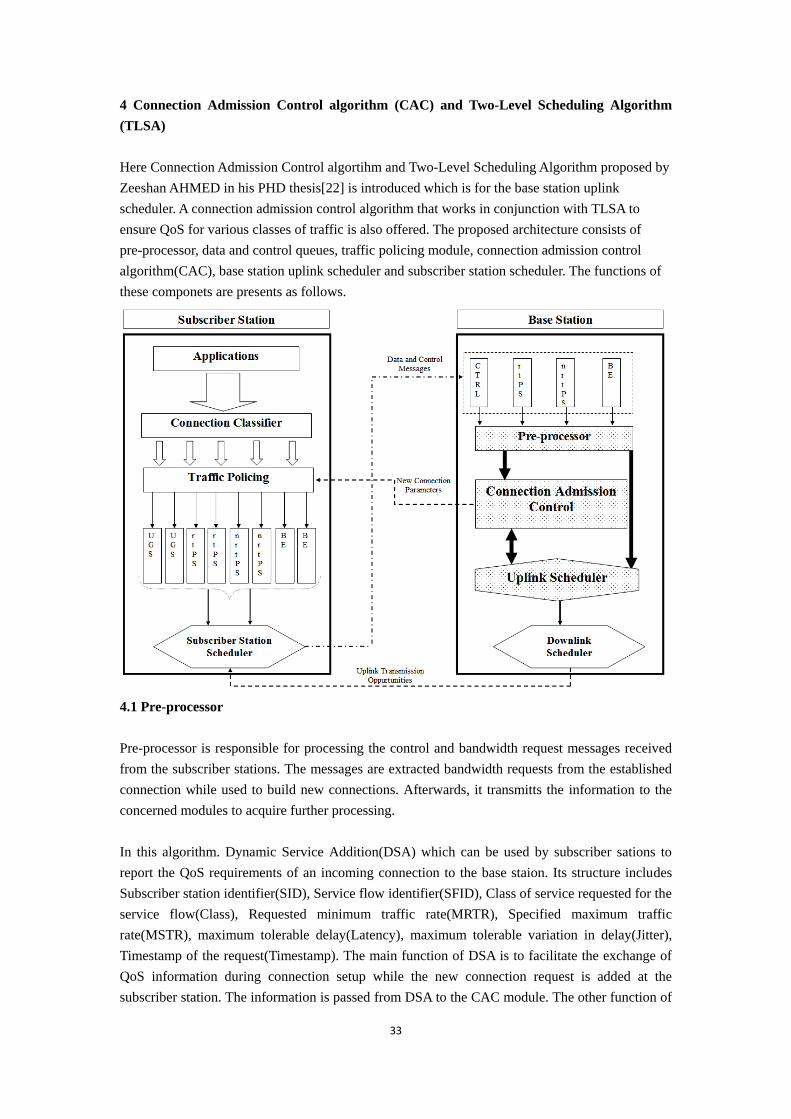
4 Connection Admission Control algorithm (CAC) and Two-Level Scheduling Algorithm

(TLSA)

Here Connection Admission Control algortihm and Two-Level Scheduling Algorithm proposed by

Zeeshan AHMED in his PHD thesis[22] is introduced which is for the base station uplink

scheduler. A connection admission control algorithm that works in conjunction with TLSA to

ensure QoS for various classes of traffic is also offered. The proposed architecture consists of

pre-processor, data and control queues, traffic policing module, connection admission control

algorithm(CAC), base station uplink scheduler and subscriber station scheduler. The functions of

these componets are presents as follows.

4.1 Pre-processor

Pre-processor is responsible for processing the control and bandwidth request messages received

from the subscriber stations. The messages are extracted bandwidth requests from the established

connection while used to build new connections. Afterwards, it transmitts the information to the

concerned modules to acquire further processing.

In this algorithm. Dynamic Service Addition(DSA) which can be used by subscriber sations to

report the QoS requirements of an incoming connection to the base staion. Its structure includes

Subscriber station identifier(SID), Service flow identifier(SFID), Class of service requested for the

service flow(Class), Requested minimum traffic rate(MRTR), Specified maximum traffic

rate(MSTR), maximum tolerable delay(Latency), maximum tolerable variation in delay(Jitter),

Timestamp of the request(Timestamp). The main function of DSA is to facilitate the exchange of

QoS information during connection setup while the new connection request is added at the

subscriber station. The information is passed from DSA to the CAC module. The other function of

34

DSA is that it can extract bandwidth request information from subcscriber station messages and to

estimate the sizes and deadlines of the packets arrived during the previous MAC frame.

Afterwards. Bandwidth Request(BR) structure is created which is to estimate values of packet

sizes and deadlines. The detail or BR is composed of SID, connection identifier(CID), Type where

0 equels to aggregate request and 1 equels to imcremental request, Size of bandwidth

requested(BRQ) and Timestamp.

For realtime connections, the deadline of the packet is the criteria for droping them in station

scheduler. Here the pre-processor module estimates the deadlines of the packets by adding the

maximum toloerable latency to the arrival time.

4.2 Queue Management

Queue Management is different at subscriber station and the base station. For subscriber station, a

separate queue is used to store data packets of each connection. The process of the data at

subscriber station is that it is passed though a packet classifier first, then stored in appropritate

queues. For example, the packets of the same connection stay in a separate queue dedicated for

that connection. For base station, each service class has an associated queue to hold bandwidth

request until processing by the uplink scheduler such as each intra-class scheduling algorithm has

only one queue to process. Pre-processor extracts a BR structure as a bandwidth request queue

which is processed in FIFO order. And the order of uplink transmission opportunities are

determined by schduling algorithm.

4.3 Traffic policing

Traffic policing is to monitor application traffic and to take appropritate actions to ensure that the

traffic of each connection is in compliance with the traffic contract. When the application data

generation rate exceeds the maximum sustained traffic rate, the module will discard traffic and

signal the action to the application layer to adapt traffic shaping which can make sure that their

traffic not be over limits and discarded.

4.4 Connection Admission Contrlo(CAC)

Connection Admission Contrlo(CAC) is a set of actions and permissions in network communi-

cation that identifies where the connection is permitted on the basis of network ability. CAC

performs the following two operations while establishing a connection: (1).The delay and mini-

mun tranffic rate of the new connection can be assured ; (2). Delay and throughput guarantees of

the existing connections are still valid.

Bandwidth stealing is used to accommodate a new connection where the minimum service levels

of existing connections should be ensured. If a new connection arrives when all the network

resources are in use, then CAC module can take the resource from the established connections to

admit the new connection such that at tleast the minimumu service level could be guaranteed to

both the new and all existing connections. The connection cannot be built when the minimum

service level is not reached. For sure, degrading the service levels of existing connections is

35

undesirable as it reduces user-satisfaction. There is an order for stealing bandwidth which are

followed by BE, nrtPS, rtPS. No bandwidth stealing can be done from UGS and ertPS classes. For

BE class, the stealing bandwidth can be stopped until the total bandwidth gets to the size of

bandwidth reserved for BE class. For nrtPS, the ending point is to reach the minimum traffic rate

of the connection. For rtPS, if there is still some need of bandwidth for the new connections, then

it is taken from rtPS class as long as conditions (1) and (2) are satisfied.

The stealing bandwidth request for BE connection can be always adimitted by the CAC module

since BE connection does not need any guarantee for thoughput and delay. The minimum

thoughput level is the main demand for nrtPS connections. Therefore, the request for nrtPS to get

bandwidth can be reached when this condition is satisfied. An rtPS connection requires guarantees

on both the minimum traffic rate and maximum delay. These two aspects have to be considered

before the operation for stealing bandwidth from it.

4.5 Two-Level Scheduling Algorithm

TLSA has two levels which are an inter-class scheduling algorthm distributing available uplink

bandwidth among various service calaases for the first level and then an class-specific algorithm

for distributing bandwidth in the specified class for the connection. The hierarchical representation

of TLSA is as follows.

4.5.1 Inter-Class Scheduling

The service class priority order suggested by IEEE 802.16 standard is valid in this inter-class

scheduling which are UGS/ertPS, rtPS, nrtPS, BE. As a result, enough resources can be provided

to each service class in this inter-class scheduling algorithm. The QoS level guaranteed by the

CAC module is ensured for all service. Lower priority flows can not disturb the bandwidth

allocation for higher priority flows. Efficient bandwidth utilization can be accomplished and no

service class starves. The details of this part is presented below.

UGS and ertPS

IEEE 802.16 standard specifies fixed-bandwidth allcatioon for UGS and ertPS. Here MRTR

equals to the fixed-bandwidth allcation. For example, αi is the MRTR of connection i , where i

∊ΔUGS∪ΔertPS which are the set of all connection of UGS and ertPS admitted by the base

station. In this algorithm, ∑ αiΔUGS and ∑ αjΔertPS units of bandwidth are allocated to UGS and

36

ertPS respectively.

nrtPS

The intra-class scheduling algorithm ensure of provding at least the MRTR to each connection.

The minimum bandwidth equals to the sum of the minimum traffic rates. The allocation of

bandwidth which is also the minimum amount of bandwidth βnrtPS can be min

(∑ αii ∊ΔnrtPS , ∑ ρii ∊ΔnrtPS |f|), ρi|f| is the total queue size of connection i at frame f.

BE

There is no minimum traffic rate for BE connections so that it is not necessary to make bandwidth

allocations. To avoid starvation of BE class, this inter-class scheduling algorithm reserves a small

part of uplink bandwidth. The bandwidth βBE should be less than or equal to ∑ ρii ∊ΔBE |f| and also

the maximum possible value of βBE which is also can be the service providers to best suit their

business model.

rtPS

Since βnrtPS and βBE units of bandwidth are reserved for nrtPS and BE, repectively, the available

for the rtPS class should be β-βUGS-βertPS-βnrtPS-βBE which is the maximum amout of bandwidth for

rtPS. However, the current bandwidth requirements of rtPS has to be considered. θrtPS is defined as

the bandwidth allocated to the rtPS class,

θrtPS|f|=min(∑ ρkk∊ΔrtPS |f|, β-∑ 𝛼𝑗j∊ΔUGS∪ΔertPS -βnrtPS-βBE)

If the bandwidth units can be left after using by rtPS, they can be utilized by nrtPS and BE classes.

As a result, actual size of bandwidth allocated to nrtPS class should be

θnrtPS|f|=βnrtPS+min(∑ ρii ∊ΔnrtPS |f|-βnrtPS, β-∑ 𝛼𝑗j∊ΔUGS∪ΔertPS -θrtPS|f|-βBE)

The maximum amount of bandwidth (θBE) available to the BE class will be

θBE=β-θrtPS|f|-θnrtPS|f|-∑ 𝛼𝑗j∊ΔUGS∪ΔertPS

4.5.2 Intra-Class Scheduling

rtPS Scheduling

Fairness To make sure the fairness for the rtPS resource allocation, Service Ratio is introduced

in this alogrithm. It is computed separately for each connection at the beginning of each

scheduling round by using Ψi|f|=∑ γi|t|

𝑓−1𝑖=1

∑ Γi|t|𝑓−1𝑖=1

, here γi|t| is bandwidth received by connection i at the

start of frame f and Γi|t| is the bandwidth requested by connection i at the start of frame f. Mean

Service Ratio is also introduced which is calculated by Ψ′|f|=∑ ∑ γi|t|𝑖∈𝛥𝑟𝑡𝑃𝑆

𝑓−1𝑖=1

∑ ∑ Γi|t|𝑖∈𝛥𝑟𝑡𝑃𝑆𝑓−1𝑖=1

. It is the ratio of total

service availed by all rtPS connections to total service requested by these connections. If

Ψi|f|>Ψ′|f|, it means that where are some connections receiving les service than connection i which

should be given a higher priority. Both Ψi and Ψ′ take bandwidth from leading flows and

37

distribute it among lagging flows. MRTR of eahc rtPS connection can be ensured by using these

two parameters. If the value of Service Ratio of eahc connection equals to Mean Service Ratio, we

can call this bandwidth allocation comletely fair which is Ψi=Ψj=Ψ′, here i,j∈ΔrtPS.

Scheduling Base station provides periodic dedicated bandwidth request opportunities to

connections. Deadline of is an important data for rtPS packet. So maximum tolerable latency of

connections is used as a criteria to determine the polling order of rtPS connection. The subscriber

station of rtPS connections which has the lowest maximum latency is polled first. So on and so

forth. As a result, the base station receives and processes the bandwidth requests in increasing

order of tolerable latency which can prioritize connections with tight delay constraints.

An rtPS connection i is allowed to receive bandwidth allocation if Ψi|f|≤Ψ′|f|. The base station

uplink scheduler always tries to allocate the bandwidth close to the total amount of Γi|f|. But

sometimes the bandwidth which is can be used is not enough to cover the bandwidth request, the

scheduler will utilize the available bandwidth in f to finish a part of Γi|f|. The other part of request

will be dealed in frame f+δi

𝛾 , here δi is the maximum tolerable latency for connection i,γ is the

duration of MAC frame in seconds.

Base station uplink scheduler uses bandwidth allocation table which is an |ΔrtPS|×δ′ to realize this

process. |ΔrtPS| is the total number of elements in ΔrtPS and δ′ equals to max(

δi

𝛾) where i ∊ΔrtPS.

Here Λ represents the bandwidth allocation table. An entry Λr,s is an ordered pair(ε,ϕ) where ε and

Φ are bandwidth allocations to connection r in frame f+s. ε is called confirmed allocation and Φ is

called tentative allocation. Confirmed allocation can be guaranteed for r in frame f+s but tentative

allocation can not which is just possibly allocated between frams f and f+s. UL_MAP can be

generated by the base station with the utilization of bandwidth allocation table. At the end of each

scheduling round, the first column of the allocation table corresponds to UL-MAP for the next

uplink subframe.

nrtPS Scheduling

The most important data to be ensured in nrtPS scheduling is minimum traffic rate for each

connection. This algorithm guarantees MRTR for each conncection fisrt, then allocates more

bandwidth for the connections which has greater queue size(backlog). Let connection v

belongs to ΔnrtPS, ρv|f| is the current bandwidth demand. For all nrtPS, the algorithm will allocate

min(ρv|f|,αv) bandwidth for v. In this way , minimum traffic rate bandwidth cab be made sure.

Afterwards, the proportion of queue sizes of each connection will be a standard to allocate

the leaving bandwidth for eahc other. The bandwidth requirements of connection u which is

denoted by ηu equals to ρu|f|- min(ρu|f|,αu). Here rnrtPS is the avilable bandwidth in frame f. This

alogrithm will deal with the residential bandwidth according to θu = min(ρu|f|,αu) +

min(rnrtPS,∑ ηvv∈nrtPS )(ηu

∑ ηvv∈nrtPS). The algorithm guarantees the minimum traffic rate and takes

backlog of each connection as weight to allocate bandwidth for more demanding connections.

38

BE Scheduling

A subscriber station with bad channel conditions use more time-slots but transfer less data

comparing to the subscriber station with good channel conditions. In this algorithm, to make a

better use of radio resource usage, it will distribute the available time-slots equally among BE

connections. For instance, C is the numer of available time-slots for BE traffic and |ΔBE| is the

number of BE connectinons. So the available slots for eahc connection will be C/ |ΔBE|. For a BE

connections w, ρw|f| is the current bandwidth request and Cw is required time-slots. This algorithm

allocates min(Cw, C/ |ΔBE|) to w. The slots will be allocated to the connection in turns to avoid the

number of available time-slots is less than BE connections number. More data will be transmitted

by the subscriber station with good channel condition within the same number of time-slots. In

this way, the scheme can prevent subscriber stations with poor channel conditions to affect the

entire network, with avoiding starvation of such subscriber stations.

5 Simulation of Two-level scheduling algorithm in QualNet

In this chapter, we provide a simulation of Two-level scheduling algorithm to check if it can have

a good performance when the physical channel condition changes. Simulation is an attempt to

model a real-life or hypothetical situation to evaluate the performance of a system, existing or

proposed, under different configurations of interest and over long periods of realtime. A design

validation tool can avoid unforeseen problems and offer desired performance levels. Meanwhile,

simulation has become a useful part of modeling many natural systems in various region to gain

insight into the peration of those systems.

A model is a representation of a system or process. A simulation model is a representation that

incorporates time and the changes taht occur over time while it is a descriptive model of a process

or system, and usually includes parameters that allow the model to be configurable, that is, to

represent a number of somewhat different system or process configurations. Simple examples

include parameters that allow a user to vary the number of workers at a workstation, the speed of a

machine or vehicle, the timing characteristics of a conveyor control system, and so on. As a

descriptive model, you can use a simulation model to experiment with, and evaluate and compare,

any number of system alternatives. Evaluation, comparison and analysis are the key reasons for

doing simulation. Prediction of system performance and identification of system problems and

their causes are the key results.

Simulation analysis can be concluded into such parts as model development, experiment design,

simulation running, data collection and analysis, conclusion formulation and decision making

complete simulation needs numbers of experiments in which some parameters change at the input

side and different values are achieved at the output side. Researchers should test their algorithms

in different condition to check if it has good performance and robustness. Understanding of

behaviors and characteristics of systems becomes very important in this situation.

Model development is very critical of the whole simulation analysis. We can configure the real

system by studying the operation of the model. Model development consists of two major

39

activities which are development of data structures to represent the data needed by the model and

translation of the modeling assumptions in the Assumptions Document into the language or

representation required by the simulation package. The simulation analyst must design data

structures that represent the data and its inter-relationships as well as fit into those allowed by the

simulation software. A good model is simpler than the the real system which can enable the

reserchers to acquire an accurate results with expected behavior of the system[23]

. Meanwhile, a

good model is an appropriate compromise between realism and simplicity. A model must be

validated extensively before its application where model validation is a strenuous process and

involves observing model output under a broad range of input. As reserched for the simulation tool

in the present markets, commercial network simulators provide a good opportunity for efficient

experimentation while offering many benifits such as validated implementation of existing

protocols, a rich infrastructure for developing new protocols, the opportunity to study large-scale

protocol interaction, easier comparison due to standardized set of result. Since Qualnet can

provide a faithful model for the 802.16 standard while equiping a user-friendly graphical

user-interface and analytical tools, we decided to use Qualnet to do the simulation ananlysis.

5.1 QualNet Introduction

QualNet provides a comprehensive environment for designing protocols, creating and animating

network scenarios, and analyzing thrie performance. QualNet is composed of the following tools:

QualNet Architect—A graphical experiment design and visualization tool.Architect has two

modes:Design mode, for designing experiments, and Visualize mode, for running and visualizing

experiments[24]

; QualNet Analyzer—A graphical statistics analyzing tool; QualNet Packet

Tracer—A graphical tool to display and analyze packet traces; QualNet File Editor—A text editing

tool; QualNet Command Line Interface—Command line access to the simulator; QualNet is a

comprehensive suite of tools for modeling large wired and wireless networks. It uses simulation

and emulation to predict the behavior and performance of networks to improve their design,

operation and management; QualNet enables users to design nex protocol models, optimize new

and existing models, design large wired and wireless networks using pre-configured or

user-designed models, analyze the performance of networks and perform what-if analysis to

optimize them.

The key features of QualNet that enable creating a virtual network enviroment are :

Speed: QualNet can support real-time speed to enable software-in-the-loop,network emulation,

and hardware-in-the-loop modeling. Faster speed enables model developers and network designers

to run multiple “what-if” analyses by varying model, network, and traffic parameters in a short

time.

Scalability: QualNet can model thousands of nodes by taking advantage of the latest hardware and

parallel computing techniques. QualNet can run on cluster, multi-core, and multi-processor

systems to model large networks with high fidelity.

Model Fidelity: QualNet uses highly detailed standards-based implementation of protocol models.

It also includes advanced models for the wireless environment to enable more accurate modeling

of real-world networks.

Portability: QualNet and its library of models run on a vast array of platforms, including Windows

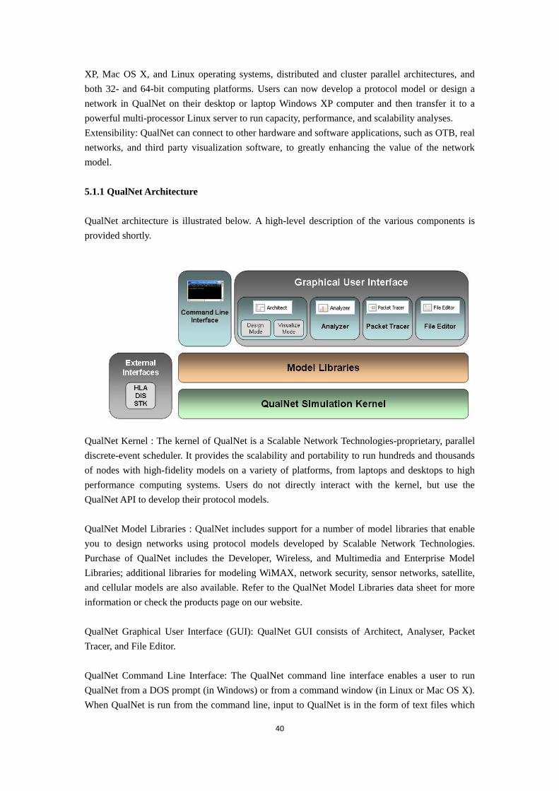
40

XP, Mac OS X, and Linux operating systems, distributed and cluster parallel architectures, and

both 32- and 64-bit computing platforms. Users can now develop a protocol model or design a

network in QualNet on their desktop or laptop Windows XP computer and then transfer it to a

powerful multi-processor Linux server to run capacity, performance, and scalability analyses.

Extensibility: QualNet can connect to other hardware and software applications, such as OTB, real

networks, and third party visualization software, to greatly enhancing the value of the network

model.

5.1.1 QualNet Architecture

QualNet architecture is illustrated below. A high-level description of the various components is

provided shortly.

QualNet Kernel : The kernel of QualNet is a Scalable Network Technologies-proprietary, parallel

discrete-event scheduler. It provides the scalability and portability to run hundreds and thousands

of nodes with high-fidelity models on a variety of platforms, from laptops and desktops to high

performance computing systems. Users do not directly interact with the kernel, but use the

QualNet API to develop their protocol models.

QualNet Model Libraries : QualNet includes support for a number of model libraries that enable

you to design networks using protocol models developed by Scalable Network Technologies.

Purchase of QualNet includes the Developer, Wireless, and Multimedia and Enterprise Model

Libraries; additional libraries for modeling WiMAX, network security, sensor networks, satellite,

and cellular models are also available. Refer to the QualNet Model Libraries data sheet for more

information or check the products page on our website.

QualNet Graphical User Interface (GUI): QualNet GUI consists of Architect, Analyser, Packet

Tracer, and File Editor.

QualNet Command Line Interface: The QualNet command line interface enables a user to run

QualNet from a DOS prompt (in Windows) or from a command window (in Linux or Mac OS X).

When QualNet is run from the command line, input to QualNet is in the form of text files which

41

can be created and modified using any text editor. Building and running scenarios with the

command line interface takes less memory and scenarios typically run faster than with the GUI.

With the command line interface the users have the flexibility to interface with visualization and

analysis tools of their choice.

QualNet External Interface: QualNet can also interact with a number of external tools in real-time.

The HLA/DIS module, which is a part of the Standard Interfaces Model Library, allows QualNet

to interact with other HLA/DIS compliant simulators and computer-generated force (CGF) tools

like OTB. The QualNet STK interface, which is a part of the Developer Model Library, provides a

way to interface QualNet with the Satellite Toolkit (STK) developed by Analytical Graphics, Inc.

(AGI) and function in a client-server environment.

5.1.2 Scenario-based Network Simulation

In QualNet, a specific network topology is referred to as a scenario. A scenario allows the user to

specify all the network components and conditions under which the network will operate. This

includes: terrain details, channel propagation effects including path loss, fading, and shadowing,

wired and wireless subnets, network devices such as switches, hubs and routers, the entire

protocol stack of a variety of standard or user-configured network components, and applications

running on the network. Most of these are optional; you can start with a basic network scenario

and specify as much detail as necessary to improve the accuracy of your network model.

5.1.3 General Approach

In general, a simulation study comprises the following phases:

The first phase is to create and prepare the simulation scenario based on the system description

and metrics of interest.

The next step is to execute, visualize, and analyse the created scenario and collect simulation

results. Simulation results can include scenario animations, runtime statistics, final statistics, and

output traces.

The last phase is to analyse the simulation results. Typically, users may need to adjust the

scenarios based on the collected simulation results. This general procedure is downstairs.

5.1.4 Files Associated with a Scenario

Input to the QualNet simulator consists of several files. For the command line interface, the input

files are text files. The main input files for command line are:

Scenario configuration file: This is the primary input file for QualNet and specifies the network

42

scenario and parameters for the simulation. This file usually has the extension “.config”.

Node placement file: This file is referenced by the scenario configuration file and specifies the

initial position of nodes in the scenario. (The node placement file may also contain the future

positions of nodes.) This file usually has the extension “.nodes”.

Application configuration file: This file is referenced by the scenario configuration file and

specifies the applications running on the nodes in the scenario.

In addition to the above three files, QualNet may use other input files. These additional files

depend upon the models specified in the configuration file and are referenced by the configuration

file. These input files are text files which can be created using any text editor. When using the

command line interface, the user has to create these files manually.

When the user creates a scenario in Architect, the major input files representing the scenario

(scenario configuration, node placement, and application configuration files) are automatically

created by Architect. The primary output file generated by a QualNet simulation run is a statistics

file, which has the extension “.stat”. This file contains the statistics collected during the simulation

run. Other output files that may be generated by QualNet include the trace file (which has the

extension “.trace”) which records packet traces, and the animation file which records the

animation trace of a scenario when the scenario is run in Architect.

Both the statistics and trace files are text files which can be viewed using any text editor. In

addition, analyser can be used to view the contents of the statistics file in a graphical, easy to

analyse manner.

5.2 Implementation of TLSA in Qualnet

The algorithms proposed for uplink scheduling can be classified into two categories:

channel-aware and channel-unaware. The channel-aware algorithms make scheduling decisions

according to channel-state information. Preference is given to subscriber stations with good

channel conditions. While, the channel-unaware algorithms make scheduling decisions according

to QoS requirements and bandwidth requests of individual connections. Both schemes have

associated advantages and drawbacks. Channel-aware schedulers maximize overall system

performance but they do not guarantee QoS for various classes of traffic. Channel-unaware

algorithms can furnish QoS to various service classes, however they ignore the variable nature of

wireless link. TLSA does not use the information of channel-state which means it belongs to

channel-unaware algorithm. Here we are going to observe that when the channel condition

becomes worse, the changeable for the performance of data transmission using TLSA will be.

First, we have to choose the parameters which can have an effect on channel-state condition such

as weather condition, noise and so on. Finally, we decided to use noise, fast fading effect and slow

fading effect to do the simulations.

5.2.1 Noise factor

In physics and analog electronics, noise is a mostly unwanted random addition to a signal; it is

called noise as a generalisation of the acoustic noise ("static") heard when listening to a weak

43

radio transmission with significant electrical noise. Signal noise is heard as acoustic noise if the

signal is converted into sound; it manifests as "snow" on a television or video image. High noise

levels can block, distort, change or interfere with the meaning of a message in human and

electronic communication.

In signal processing or computing noise can be considered random unwanted data without

meaning; that is, data that is not being used to transmit a signal, but is simply produced as an

unwanted by-product of other activities. "Signal-to-noise ratio" is sometimes used to refer to the

ratio of useful to irrelevant information in an exchange.

Noise figure (NF) and noise factor (F) are measures of degradation of the signal-to-noise

ratio(SNR), caused by components in a radio frequency (RF) signal chain. It is a number by which

the performance of a radio receiver can be specified. The noise factor is defined as the ratio of the

output noise power of a device to the portion thereof attributable to thermal noise in the input

termination at standard noise temperature T0 (usually 290 K). The noise factor is thus the ratio of

actual output noise to that which would remain if the device itself did not introduce noise, or the

ratio of input SNR to output SNR. The noise figure is simply the noise factor expressed in decibels

(dB). In QuelNet, we can change the value of Noise figure to make a difference on the physical

channel. The Human-made noise in the city and countryside is from 0-100dB.

5.2.2 Fading factor

In wireless communications, fading is deviation of the attenuation affecting a signal over certain

propagation media. The fading may vary with time, geographical position or radio frequency, and

is often modeled as a random process. A fading channel is a communication channel comprising

fading. In wireless systems, fading may either be due to multipath propagation, referred to as

multipath induced fading, or due to shadowing from obstacles affecting the wave propagation,

sometimes referred to as shadow fading.

The presence of reflectors in the environment surrounding a transmitter and receiver create

multiple paths that a transmitted signal can traverse. As a result, the receiver sees the superposition

of multiple copies of the transmitted signal, each traversing a different path. Each signal copy will

experience differences in attenuation, delay and phase shift while travelling from the source to the

receiver. This can result in either constructive or destructive interference, amplifying or

attenuating the signal power seen at the receiver. Strong destructive interference is frequently

referred to as a deep fade and may result in temporary failure of communication due to a severe

drop in the channel signal-to-noise ratio.

A common example of multipath fading is the experience of stopping at a traffic light and hearing

an FM broadcast degenerate into static, while the signal is re-acquired if the vehicle moves only a

fraction of a meter. The loss of the broadcast is caused by the vehicle stopping at a point where the

signal experienced severe destructive interference. Cellular phones can also exhibit similar

momentary fades.

44

Fading channel models are often used to model the effects of electromagnetic transmission of

information over the air in cellular networks and broadcast communication. Fading channel

models are also used in underwater acoustic communications to model the distortion caused by the

water. Mathematically, fading is usually modeled as a time-varying random change in the

amplitude and phase of the transmitted signal.

The terms slow and fast fading refer to the rate at which the magnitude and phase change imposed

by the channel on the signal changes. The coherence time is a measure of the minimum time

required for the magnitude change of the channel to become uncorrelated from its previous value.

Slow fading arises when the coherence time of the channel is large relative to the delay constraint

of the channel. In this regime, the amplitude and phase change imposed by the channel can be

considered roughly constant over the period of use. Slow fading can be caused by events such as

shadowing, where a large obstruction such as a hill or large building obscures the main signal path

between the transmitter and the receiver. The received power change caused by shadowing is often

modeled using a log-normal distribution with a standard deviation according to the log-distance

path loss model.

Fast fading occurs when the coherence time of the channel is small relative to the delay constraint

of the channel. In this regime, the amplitude and phase change imposed by the channel varies

considerably over the period of use. For fast fading, we decided to use Rayleigh fading model in

the QuelNet.

Rayleigh fading is a statistical model for the effect of a propagation environment on a radio signal,

such as that used by wireless devices. Rayleigh fading models assume that the magnitude of a

signal that has passed through such a transmission medium (also called a communications channel)

will vary randomly, or fade, according to a Rayleigh distribution — the radial component of the

sum of two uncorrelated Gaussian random variables.

Rayleigh fading is viewed as a reasonable model for tropospheric and ionospheric signal

propagation as well as the effect of heavily built-up urban environments on radio signals. Rayleigh

fading is most applicable when there is no dominant propagation along a line of sight between the

transmitter and receiver. If there is a dominant line of sight, Rician fading may be more applicable.

Rayleigh fading is a reasonable model when there are many objects in the environment that scatter

the radio signal before it arrives at the receiver. The central limit theorem holds that, if there is

sufficiently much scatter, the channel impulse response will be well-modelled as a Gaussian

process irrespective of the distribution of the individual components. If there is no dominant

component to the scatter, then such a process will have zero mean and phase evenly distributed

between 0 and 2π radians. The envelope of the channel response will therefore be Rayleigh

distributed.

Rayleigh fading is also called multipath fading in the mobile radio environment. Speed of

reflecting objects can induce their own Doppler shift in the reflected wave. Doppler frequency or

Doppler shift is given by fd=(1/λc)Vmcos 𝜃 , where λc is the wavelength of the carrier signal, Vm is

the relative velocity of the mobile, the angle θ is between the motion of the mobile and direction

45

of arrival of the scattered waves, and Vmcos 𝜃m represents the velocity component of the motion

of the mobile in the direction of the incoming signal. Here we can change the maximum velocity

in the QualNet and choose the range from 10-60 meter/second.

5.2.3 Shadowing factor

For slow fading, shadowing model is chosen in QualNet. The telecommunication conditions may

vary as one turns a corner, moves behind a large building, or enters a building. This can be called

shadowing or large-scale fading while it belongs to slow fading.

Large-scale variations caused by shadowing of obstacles are shown to follow a log-normal

distribution, which means that when measured in dB they follow a Gaussian distribution.

Consequently shadowing effects they are usually incorporated into path loss estimates by the

addition of a zero-mean Gaussian random variable, with standard deviation σ: N(0,σ), where σ is

often estimated by empirical measurements. Commonly accepted values for σ are between 6 dB

and 12 dB.

Measured values of σ itself seem to display Gaussian distribution as well, in their variations from

one area to another, and depend on the radio frequency, the type of environment (rural, suburban,

or urban), base station and subscriber station height. Many measurement campaigns have been

conducted and reported in the literature, as summarized in table bellows:

Source Frequency(GHz) Path Loss

Exponent n

Ο(dB) Comments

Seidel[25]

0.9 2.8 9.6 Suburban(Stuttgart)

Erceg[26]

1.9 4.0 9.6 Terrain-category B

Feuerstein[27]

1.9 2.6 7.7 Med.antenna height

Durgin[28]

5.8 2.93 7.85 [28]Fig.7,residential

Porter[29]

3.7 3.2 9.5 Some denser urban

Rautiainen[30]

5.3 4.0 6.1 [30]Fig.3,4

Here we use the shadowing model in QuelNet and the range of shadowing mean is from 6dB to

12dB.

5.3 Analyse of the simulation

TLSA is implemented at base station. The function MacDot16ScheduleUlSubframe obeys the

strict priority which is UGS>ertPS>rtPS>nrtPS>BE and WFQ based scheduling. Here TLSA is

modified in this function to replace strict priority and WFQ algorithms in files “mac_dot16_sch.h”

and “mac_dot16_sch.cpp”. Also code is added in “mac_dot16_ss.cpp” to drop the expired packets

from data queues.

Four performance metrics are used to analyse the performance of the proposed scheduling scheme.

Throughput: The total units of data transmitted in duration Δt divided by Δt.

End-to-end Delay: The average delay observed by packets from source to destination. It includes

queuing delay and propagation delay.

46

Packet Loss Ratio: The number of packets lost to the total number of packets sent by the sender.

Jitter: The undesired deviation from true periodicity of an assumed periodic signal.

The simulation experiments are made of three subscriber stations and one base station. All the SSs

are sending CBR data to this base station at the same time. All the data types are set to rtPS. The

total uplink channel capacity is set to 1Mbps. Two-ray ground reflection is used as radio

propagation model. Frame duration is 20ms while TDD downlink duration is 10ms. The antenna

model is omni antenna. And I set the temperature as 290K. Link adaptation and packing are enable.

Each subscriber station sends 10000 items totally and the item size is 512 bytes. The CBR interval

is 0.1 seconds and the simulation experiment starts at 1 seconds and ends at 1000 seconds. The

total simulation time is 1000 seconds. The fading model is unused when the experiments are for

noise factor and shadowing factor changing. Shadowing mean is set to 4dB in the simulation for

acquiring performance for noise factor and fading factor. And the noise is set to 10dB in fading

and shadowing experiments. As presented before, the fading factor ranges from 10dB and 60dB

every 5dB. The noise factor increase from 10dB to 100dB with the interval of 10dB. For the

shadowing factor experiment, the range is 6dB to 12dB. The experiment with each parameter is

simulated 30 times. After calculating the data, we have got 12 graphs.

47

However, these results are very difficult to observe the performance. I surmise there are some

mistakes in the initial set which leads to it. Finally there are three main problems affecting the

statistics:

1. The start time should be delayed a little for proper routing. Otherwise there would be some

packets loss in the start and therefore results would not be very accurate.

48

2. Simulation end time should be greater than the end time of data generation. In this case, the

packets in the queue could be scheduled.

3. Data generation rates should be close to total uplink capacity, If the data generation rate is equal

to available capacity, then this is full load scenario which can be also considered as a worst-case

scenario. For simulation experiment, network must be tested under worst-case scenario to ensure

their satisfactory operation under full system load. The data generation rate can be calculated as

packet size×8×(1/packets generation interval). Here we can modify either packet size or packet

generation interval to change data generation rate. Here the value of it is 512×8×(1/0.1)=40960bps

which is very far from total uplink capacity which makes the result not accurate.

As a correction, I set the start time into 10 seconds and end time into 110s while the interval is

0.01s. The total simulation time is 200 seconds. The item size is increased to 1024 bytes. Then I

did the simulation experiments again and update all the data. The new graphs with new statistics

are presented below.

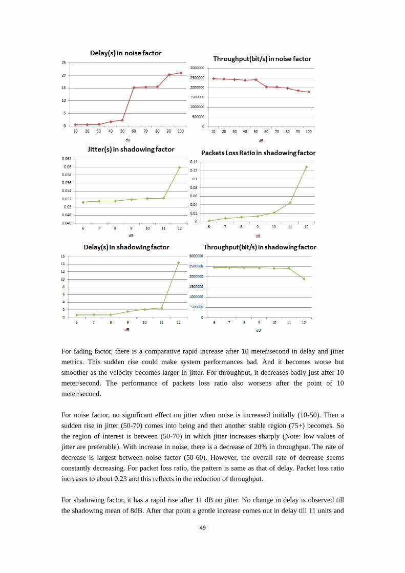
49

For fading factor, there is a comparative rapid increase after 10 meter/second in delay and jitter

metrics. This sudden rise could make system performances bad. And it becomes worse but

smoother as the velocity becomes larger in jitter. For throughput, it decreases badly just after 10

meter/second. The performance of packets loss ratio also worsens after the point of 10

meter/second.

For noise factor, no significant effect on jitter when noise is increased initially (10-50). Then a

sudden rise in jitter (50-70) comes into being and then another stable region (75+) becomes. So

the region of interest is between (50-70) in which jitter increases sharply (Note: low values of

jitter are preferable). With increase in noise, there is a decrease of 20% in throughput. The rate of

decrease is largest between noise factor (50-60). However, the overall rate of decrease seems

constantly decreasing. For packet loss ratio, the pattern is same as that of delay. Packet loss ratio

increases to about 0.23 and this reflects in the reduction of throughput.

For shadowing factor, it has a rapid rise after 11 dB on jitter. No change in delay is observed till

the shadowing mean of 8dB. After that point a gentle increase comes out in delay till 11 units and

50

then a sudden jump appears in delay. This sudden rise in delay could degrade system

performances. Sudden drop in throughput is observed after shadowing mean of 11 units.

Throughput is quite good between 6 and 11 units with little packet drop. The packet loss ratio

reaches a maximum of 0.13.

6. Conclusion

The TLSA algorithm has a relative bad performance when the fast fading effect increases. But in

the normal range of shadowing effecting in humans’ life, it can deliver a good communication for

the users as well as noise factor increases. Since it does not use the channel condition information,

its performance is more than fair.

Also we have compared the technology in WiMAX and LTE who are main the competitors in the

4G communication market. They also utilize some common technique such as OFDM and MIMO.

There is hot discussion about merge or competition about them nowadays. Just because of the

similarities between them, more researchers are supporting the merging opinion. However, the

technique used by them is not only the factor to be considered but also the market decision which

is more important sometime. Merging WiMAX and LTE seems too difficult to realize. The

competition between these two technologies cannot be avoided. LTE has a big advantage that

more telecommunication operators decide to use it as their 4G technology finally. But it cannot

mean that the WiMAX is the loser in this 4G match. Obviously, LTE is the successor of the

cellular technology such as UMTS/WCDMA/HSPA/ and CDMA2000 3G while WiMAX is

mainly used in broadband wireless connection and backhaul. As the expend of WiMAX is much

smaller than LTE, many developing countries can choose WiMAX instead of LTE which is easier

to be accomplished.

WiMAX and LTE have many differences on their way of technology developing, but they all fit in

the need of wireless communication for users. Apparently, they have some specific advantages and

disadvantages. However, it is more important to create a large “net” where multiple technique can

be used to get a goal that users could have a better experience.

51

Reference

[1]Frank Ohrtman, “WiMAX Handbook”, McGraw-Hill Communications Companies, 2005

[2]Jeffrey G. Andrews, Arunabha Ghosh, Rias Muhamed, “Fundamentals of WiMAX”, Pearson

Education, February 2007

[3]Y. Ahmet Sekercioglu, Milosh Ivanovich, Alper Yegin, “A survey of MAC based QoS

implementations for WiMAX networks”, Computer Network(2009)

[4]R. Farhadi, V. T. Vakili, and S. S. Moghadam, “A comparative study of scheduling algorithms

for OFDMA-based WiMAX networks,” 2011 IEEE 3rd International Conference on

Communication Software and Networks, no. Cid, pp. 355–359, 2011.

[5]R. Jain, and a K. Tamimi, “Scheduling in IEEE 802.16e mobile WiMAX networks: key issues

and a survey,” IEEE Journal on Selected Areas in Communications, vol. 27, no. 2, pp. 156–171,

2009.

[6]Chou, “Two-Tier Scheduling Algorithm for Uplink Transmissions in IEEE 802.16 Broadband

Wireless Access Systems,” 2006 International Conference on Wireless Communications

Networking and Mobile Computing, pp. 6–9, 2006.

[7]Kim, Seungwoon and Yeom, Ikjun, “TCP-aware Uplimk scheduling for IEEE 802.16”. IEEE

Communication Letter, Feb., 2007.

[8]Zeynep Yurdakul, Sema Oktug, “A Hierarchical Channel-Aware Uplink Scheduler For WiMAX

Based Stations”, 2010 Sixth Advanced International Conference on Telecommunications, IEEE

computer societ y, pp. 398-403.

[9]E. Limouchi, S. T. Branch, A. Salajeghe, M. Pourmina, and A. Zehni, “An Intra-Class

Channel-Aware Scheduling in IEEE,” Network, IEEE, vol. 1, no. 8, pp. 323–325, 2011.

[10]D. Astely, E. Dahlman, a Furuskar, Y. Jading, M. Lindstrom, and S. Parkvall, “LTE: the

evolution of mobile broadband,” IEEE Communications Magazine, vol. 47, no. 4, pp. 44–51,

2009.

[11]P. Development and T. Challenges, “Agilent 3GPP Long Term Evolution : System Overview,

Product Development and Test Challenges,” 2009.

[12]M. Alasti and B. Neekzad, “Quality of Service in WiMAX and LTE Networks,”

Communications Magazine, IEEE, vol. 48, no. May, pp. 104–111, 2010.

[13]F. D. Calabrese, C. Rosa, M. Anas, P. H. Michaelsen, K. I. Pedersen, P. E. Mogens “Adaptive

Transmission Bandwidth Based Packet Scheduling for LTE Uplink”, Nokia Siemens Networks,

Denmark

[14]T.E. Kolding, “QoS-Aware Proportional Fair Packet Scheduling with Required Activity

Detection”, IEEE 64th Vehicular Technology Conference, September 2006.

[15]Sunggu Choi, Kyungkoo Jun, Yeonseung Shin, Seokhoon Kang, Byoungjo Choi. “MAC

Scheduling Scheme for VoIP Traffic Service in 3G LTE” Vehicular Technology Conference, 2007.

VTC-2007 Fall. 2007 IEEE 66th, 1441—1445

[16]M. Anas, C. Rosa, F. D. Calabrese, K. I. Pedersen, and P. E. Mogensen, “Combined

Admission Control and Scheduling for QoS Differentiation in LTE Uplink,” 2008 IEEE 68th

Vehicular Technology Conference, vol. 68, no. September, pp. 1–5, 2008.”

[17]K. Etemad and I. Corporation, “Overview of Mobile WiMAX Technology and Evolution,”

Communications magazine, IEEE, vol. 46, no. October, pp. 31–40, 2008.

[18]3GPP, “3GPP System Architecture Evolution: Report on Technical Options and

52

Conclusions(Release 8)”, TR 23.882.V8.0.0(2008-09)

[19]3GPP TS 36.300 V8.4.0(2008-03)

[20]Fan Wang et al., “Mobile WiMAX Systems: Performance and Evolution”, IEEE

Communications Magazine, Volume 46, No.10, October 2008

[21]L. Li and S. Shen, “End-to-End QoS Performance Management Across LTE Networks,”

Network Operations and Management Symposium (APNOMS), 2011 13th Asia-Pacific, vol. 2011,

pp. 1–4, 2011.

[22] Zeeshan Ahmed, “Quality of Service in WiMAX for Multimedia Services”, Phd thesis, June

2013

[23]Lee Breslau, Deborah Estrin, Kevin Fall, Sally Floyd, John Heidemann, Ahmed Helmy, Polly

Huang, Steven McCanne, Kannan Varadhan, Ya Xu, et al. “Advances in network simulation.

Computer”, 33(5):59–67, 2000. 124,125

[24]Qualnet Simulator. 5.0, qualnet 5 users guide scalable network technologies.Inc 2010, 2010.

126, 128, 224

[25]V.S. Abhayawardhana, I.J. Wassell, D. Crosby, M.P. Sellars, and M.G. Brown, “Comparison

of empirical propagation path loss models for fixed wireless access systems”, in Vehicular

Technology Conference, Spring 2005, Volume 1, pp. 73–77, 30 May – 1 June 2005.

[26]V. Erceg, L.J. Greenstein, S.Y. Tjandra, S.R. Parkoff, A. Gupta, B. Kulic, A.A. Julius, R.

Bianchi, “An Empirically Based Path Loss Model for Wireless Channels in Suburban

Environments”, in IEEE Journal on Selected Areas in Communications, Volume 17, No. 7, July

1999.

[27]M.J. Feuerstein, K.L. Blackard, T.S. Rappaport, S.Y. Seidel, H.H. Xia, “Path loss, Delay

Spread, and Outage Models as Functions of Antenna Height for Microcellular System”, in IEEE

Transactions on Vehicular Technology, Vol. 43, No 3, pp. 487-498, August 1994.

[28]G.D. Durgin, T.S. Rappaport, and H. Xu, “Measurements and Models for Radio Path Loss In

and Around Homes and Trees at 5.85 GHz”, in IEEE Transactions on Communications, Volume

46, No 11, pp. 1484–1496, November 1998.

[29]J.W. Porter, I. Lisica, G. Buchwald, “Wideband mobile propagation measurements at 3.7 GHz

in an urban environment”, in IEEE Antennas and Propagation Society International Symposium,

Volume 4, pp. 3645–3648, 20-25 June 2004.

[30]T. Rautiainen, K. Kalliola, J. Juntunen, “Wideband radio propagation characteristics at 5.3

GHz in suburban environments”, in Proc. IEEE 16th International Symposium on Personal, Indoor

and Mobile Radio Communications, 2005, PIMRC 2005, Volume 2, pp. 868–872, 11–14

September.