Performance Analysis of a Header Compression Protocol:

The ROHC Unidirectional Mode

Alain Couvreur∗, Louis-Marie Le Ny†, Ana Minaburo∗,

Gerardo Rubino†, Bruno Sericola†, and Laurent Toutain∗

Abstract

The performance of IPv6 in the radio link can be improved using header compression

algorithms. The 3GPP (3rd Generation Partnership Project) consortium in its techni-

cal specification has adopted the ROHC (RObust Header Compression) protocol of the

IETF (Internet Engineering Task Force) standard track for real-time applications using

RTP/UDP/IPv6 and UDP/IPv6. This paper presents the analysis of the proposed stan-

dard ROHC deployed in an UMTS radio link and discusses different schemes to increase

compression performance. The results are based on our IPv6 implementation of the RO-

HC header compression algorithm and on a simple and accurate analytical model used to

evaluate the packet loss probability.

Keywords :ROHC, Performance evaluation, IPv6, UMTS

1 Introduction

The UMTS (Universal Mobile Telecommunication System) is the third generation (3G) mobile

network under development in the 3GPP Consortium. The scenario will be of a convergence∗ENST Bretagne, BP 78, 2 rue de la Chataigneraie, 35512 Cesson Sevigne Cedex, France.

{Alain.Couvreur}{Anacarolina.Minaburo}{Laurent.Toutain}@enst-bretagne.fr†IRISA, Campus de Beaulieu, 35042 Rennes Cedex, France.

{Louis-Marie.Leny}{Gerardo.Rubino}{Bruno.Sericola}@irisa.fr

1

between mobile telephony and Internet, where a wide variety of services independent of the user

location will be provided. UMTS is expected to provide many services based on the Internet or

IP-based services. However, the use of IP will mean large overheads, and will take a significant

amount of bandwidth, which is already scarce in cellular links. Moreover, the use of IPv6

flows for data transmissions in Releases 4 and 5 of UMTS will degrade the situation, as the

overhead bytes in IPv6 are larger. Hence, there is a need to compress the large headers and

save some valuable radio resources. In the UMTS reference protocol architecture, a special

layer (PDCP: Packet Data Convergence Protocol) dedicated to header compression has been

introduced. The header compression is a scheme that removes (ideally all) the redundant

information from the header. Existing header schemes do not perform well over cellular links

due to the high BER (Bit Error Rate), around 10−2 to 10−3, and the high RTT (round trip

time), around 200ms, of the radio channel. In this scenario, a valid solution is represented by

ROHC (Robust Header Compression); it has been proposed by the IETF (Internet Engineering

Task Force) ROHC working group. ROHC aims at providing a high compression efficiency and

a high robustness and can be used in the PDCP layer. In order to investigate the behavior

of header compression for real-time applications in UMTS architecture, we have implemented

ROHC header compression and have studied it on a simulated model of the error conditions and

the long round trip time that prevail in the radio link. We present ROHC header compression

algorithm and show how it works with UMTS. In the following sections, we discuss the existing

header compression schemes and then explain the ROHC header compression protocol. Next, we

discuss the implementation of the protocol and develop an analytical model which is validated

by the implementation and which allows us to compute the packet loss probability for various

values of the input parameters. The analytical model represents the ROHC Unidirectional

mode that is used at the beginning of each transmission and well adapted for some multimedia

or military applications. The satellite links and multicast transmission are also concerned.

2

2 Header Compression

The problem of the performance of the IP protocol over a low bandwidth link has been studied

since 1984 with the Thin-wire protocol specified by Faber and Delp (1994). Van Jacobson

(1990) proposed a mechanism based on the header redundancy information, which compressed

the 40 bytes of the TCP/IPv4 header to 3-6 bytes. There are other propositions for the

different protocol headers based on redundancy, as the CTCP (IP Header Compression) header

mechanism, proposed by Degermark, Nordgren and Pink (1999), which manages a wide variety

of streams and gives particular attention to IPv6. The CRTP (Compressing IP/UDP/RTP

Headers for Low-Speed Serial Links) header mechanism (Casner and Jacobson (1999)) is a

detailed specification for RTP (the basic protocol for real-time data streams) compression.

Previous studies have demonstrated that the performance of these protocols is still quite poor

in wireless links. The next generation of header compression mechanisms aims to add a robust

and efficient compression scheme that can be used in a low bandwidth link with significant error

rate. An Algorithm to improve the performance and robustness for TCP/IP flows was proposed

by Degemark, Nordgren and Pink (1999) who suggested a strategy to recover from the loss of

compression synchronization, which occurs due to high BER. A second algorithm to further

reduce the probability of synchronization loss was presented by Perkins and Mutka (1997)

(PEHRC). These schemes were further improved by Giovanardi et al. (2000) who proposed

two retransmission strategies (ABP-SCS) and (ABP-DCS), in order to reduce the TCP/IP

header synchronization loss in an UMTS radio link. The new contributions for TCP/IP header

compression are TAROC (Liao et al. (2001)), EPIC (Price et al. (2002)) and ROHC+ (Boggia,

Camarda and Squeo (2002)). TAROC’s goal is the limitation of error propagation using TCP

congestion window tracking. EPIC uses a variant of Huffman encoding to produce a set of

compressed header formats. ROHC+ proposes a new profile and an algorithm for compressing

TCP stream within the ROHC framework. Many contributions have been proposed for the

IP/UDP/RTP protocol stack, like the adapted header compression for real time multimedia

application (ACE) (Le at al. (2000)), the header compression using keyword packets (Miyazaki

et al. (2000)), or the header compression based on Checksum (ROCCO) (Jonsson at al. (1999)).

3

These three contributions are the basis for the header compression standard ROHC (Robust

Header Compression) described in RFC 3095 (Bormann et al. (2001)).

3 The ROHC Protocol

ROHC header compression algorithm was conceived to reduce the header sizes of IP packets

to be sent through a cellular link, which is characterized, by high BER, long RTT (Round

Trip Time) and residual errors. In order to compress the Header, ROHC mechanism makes

a classification of the header fields. This analysis is based on how the values in the header

fields change during the transmission of a stream. These fields are separated and assigned

to the static and the dynamic chain of the compressed header packets. Static refers to the

information which remains more or less constant during the lifetime of the stream and dynamic

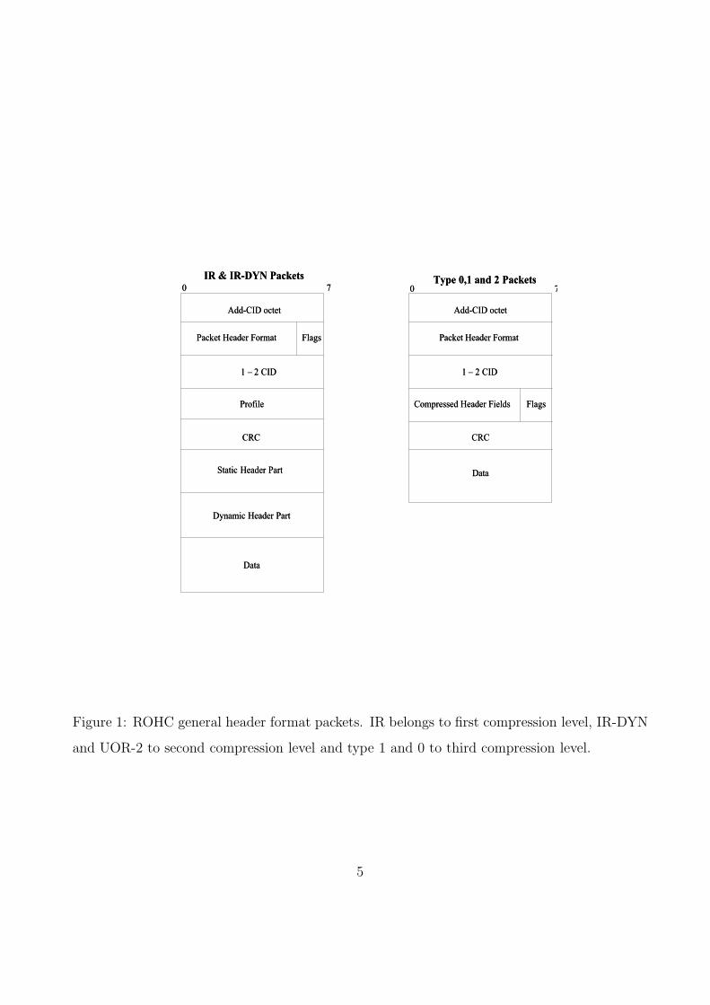
refers to the information which may change but whose change pattern may be known. ROHC

uses different header format packets to establish the information in the decompressor, see Figure

1. First, the static information is sent to the decompressor and after the compression level is

increased by sending just the dynamic information or the compress header fields variation,

which is the encoding value of the timestamp, RTP “more” flag and the sequence number. The

principle of ROHC is to send the minimal information with high robustness. One key element

here is CRC (Cyclic Redundancy Check) that is computed over the original header fields before

compression. The decompressor then verifies the CRC after decompressing the header and

checks whether it has received the correct information or if the information has been corrupted

due to transmission errors in the link.

3.1 ROHC Context

ROHC uses a context maintained between compressor and decompressor to store the informa-

tion about the header stream. This context contains the last correct update of the original

header and the redundant information in the stream. This context is kept both in the compres-

sor and in the decompressor in order to ensure the robustness of the mechanism. Each time a

value in the context changes, the context is updated. If the context is lost due to transmission

4

Add-CID octet

Packet Header Format Flags

Profile

CRC

Static Header Part

Dynamic Header Part

1 – 2 CID

Data

Add-CID octet

Packet Header Format

Compressed Header Fields Flags

CRC

1 – 2 CID

Data

IR & IR-DYN Packets Type 0,1 and 2 Packets0 7 0 7

Add-CID octet

Packet Header Format Flags

Profile

CRC

Static Header Part

Dynamic Header Part

1 – 2 CID

Data

Add-CID octet

Packet Header Format

Compressed Header Fields Flags

CRC

1 – 2 CID

Data

IR & IR-DYN Packets Type 0,1 and 2 Packets0 7 0 7

Figure 1: ROHC general header format packets. IR belongs to first compression level, IR-DYN

and UOR-2 to second compression level and type 1 and 0 to third compression level.

5

errors then there is no synchronization between the compressor and the decompressor. The

decompressor then can request for the context update through the possible use of acknowledge-

ments. Each flow in a channel has its context, which is identified by a CID (Context Identifier)

which is a number that differentiate the flows in a channel, and the context in compressor and

decompressor.

3.2 ROHC Profiles

The profiles are used to define different types of header streams. The decompressor can define

the stream type by looking at the profile. Currently five profiles have been standardized but

this could change in the future: Profile 0, without compression. When this profile is used, only

the ROHC Context Identifier is added to each packet to let the decompressor know that the

stream is not compressed. ROHC defines 4 profiles:

• Profile 1, IPv4/v6/UDP/RTP header compression. This is the generic profile; this profile

compresses three-header protocol (IPv4/v6/UDP/RTP).

• Profile 2, IPv4/v6/UDP header compression. This is a variation from profile 1, where the

compression is only applied for the UDP/ IPv4/v6 headers.

• Profile 3, IPv4/v6/ESP header compression. This profile compresses the ESP/ IPv4/v6

protocol.

• Profile 4, IPv4/v6 header compression. This profile compresses only the IPv4/v6 header.

3.3 ROHC Negotiation

The first phase of ROHC protocol is a negotiation. In this phase, the compressor and the

decompressor learn about the different characteristics of the link and the parameters that

they will use for compression. Negotiation is made while establishing a channel. A channel

is a connection between two nodes. Each channel has a compressor and a decompressor at

each side, with the possibility of it being either bi-directional or unidirectional. The present

6

solution (Jonsson (2002)) is for an Internet network where each IP interface in the IP layer

can have multiple channels, each one being bi-directional or unidirectional. The present ROHC

negotiation establishes the following parameters: MAX CID: the maximum CID that can be

used. MAX Header: the largest header that can be compressed. MRRU (Maximum Received

Reconstructed Unit): when segmentation is used, it helps to know the maximal size of the

segment in bytes. Sub-options: there can be zero or several sub-options. Until now, only one

sub-option has been specified: The Profile. It informs about the profiles that are supported.

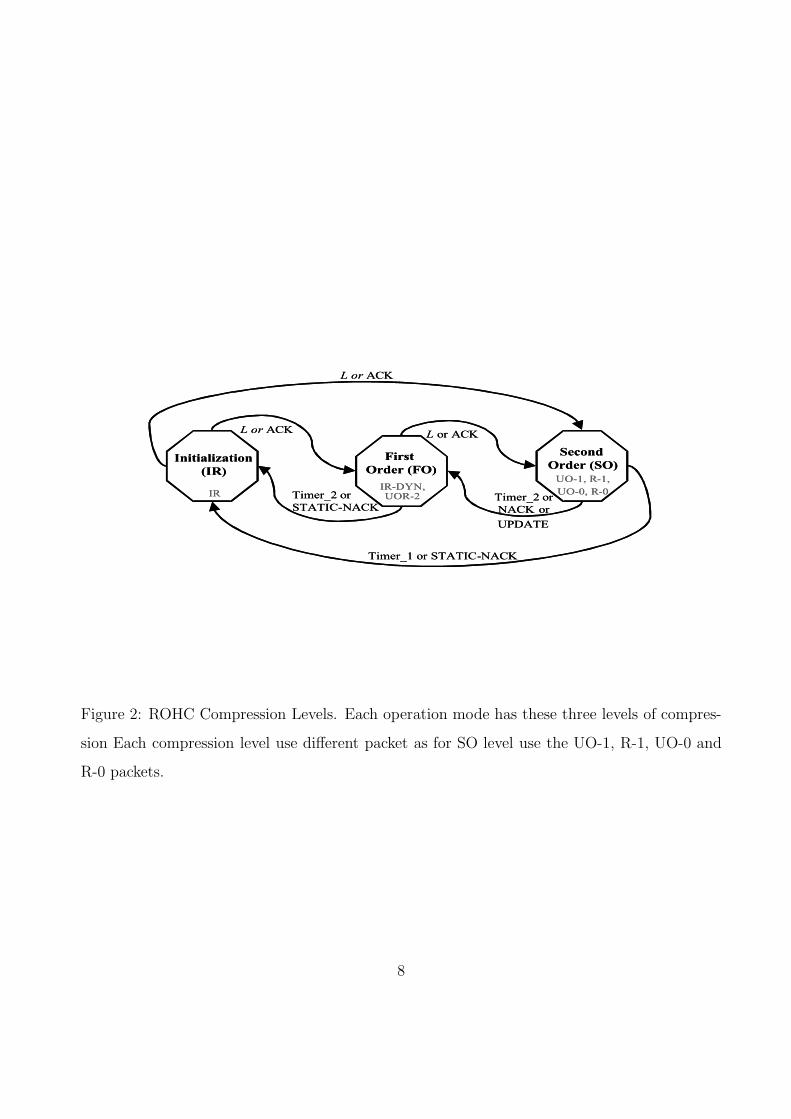
3.4 Compression Levels

ROHC has three compression levels: Initialization and Refresh (IR), First Order (FO) and Sec-

ond Order (SO). Each compression level in each operation mode uses different header types, as

shown inside the octagons in Figure 2. Forward and backward transitions to the different com-

pression levels depend on the operation mode; there are three operation modes. The compressor

always sends the header format packet that fits the information needed for decompressor.

The size of the compressed header depends on the compression level and the header infor-

mation required by the decompressor. In the first level of compression IR, the header size is

between 48 to 130 bytes; In the First Order, the compressed headers have a size between 3 to

84 bytes. In the last compression level (SO), the header is compressed up to just one byte.

3.5 Operation Modes

The different operation modes allow the compressor to change from one mode to another based

on the link characteristics and the performance requirements. Each operation mode has its

own behavior. In Unidirectional (U) mode the compressor operates over links where feedbacks

are not possible. The compressor uses a confidence system, L to base its confidence about

decompressor status. This system sends the same header format packet L times to transit

forward to the next compression levels. U-mode also uses two timers and keeps on coming

back to initial compression levels when timer expires or when there is an update in the header

information. One timer is used to come back to IR compression level, Timer 1 (IR TIMEOUT)

7

Initialization

(IR)

First

Order (FO)

Second

Order (SO)

IRIR-DYN,UOR-2

UO-1, R-1,

UO-0, R-0

L or ACK

L or ACKL or ACK

Timer_2 or

NACK or

UPDATE

Timer_2 or

STATIC-NACK

Timer_1 or STATIC-NACK

Initialization

(IR)

First

Order (FO)

Second

Order (SO)

IRIR-DYN,UOR-2

UO-1, R-1,

UO-0, R-0

L or ACK

L or ACKL or ACK

Timer_2 or

NACK or

UPDATE

Timer_2 or

STATIC-NACK

Timer_1 or STATIC-NACK

Figure 2: ROHC Compression Levels. Each operation mode has these three levels of compres-

sion Each compression level use different packet as for SO level use the UO-1, R-1, UO-0 and

R-0 packets.

8

and other is used to come back to FO compression level, Timer 2 (FO TIMEOUT). The bi-

directional optimistic (O) mode is very similar to the U-mode but the decompressor can also

send negative acknowledgements. This mode does not use the two timers, but it uses the

confidence system, L. The compressor goes downward to the initial compression levels on the

receipt of negative feedbacks. There are two kinds of negative feedbacks: NACK, that force

compressor to go to FO compression level, and the STATIC-NACK that forces it to go to

IR compression level, see Figure 2. If the compressor receives a header that will update the

entire context or if a SO packet cannot communicate the changes then, it goes down to FO

or IR level of compression. The bi-directional reliable operation (R) mode works only with

the acknowledgements received from the decompressor. Each time the compressor receives an

ACK/NACK; the compressor changes the compression level. It goes to the IR compression level

if a STATIC-NACK is received, see Figure 2. Here, a secure reference principle is also enforced

in both compression and decompression logic. The principle means that only a compressed

packet carrying a seven or eight-bit CRC can update the decompression context and can be

used as a reference for subsequent decompression.

3.6 ROHC Decompressor

The decompressor has a state machine based on the context state (see Figure 3). The decom-

pressor has three states. The first state is No Context (NC), the decompressor stays initially

where there is no context and reached it when the context is lost. In this state only the IR

header, format packets are decompressed and any other header format packet is dropped. The

decompressor changes to Full Context (FC) state as soon as correct decompression of a header

takes place (verified by CRC) or if the context is established. The Static Context (SC) state

is not reached except when there is an error and the dynamic part of the header is lost. The

decompressor then waits for a timer to be expired in U-mode. In the other modes, it sends a

NACK to the compressor for getting a FO compression level packet. The decompressor uses a

”k out of n” failure rule, where k is the number of packets received with an error in the last

n transmitted packets. This rule is used in the state machine of the decompressor in order to

9

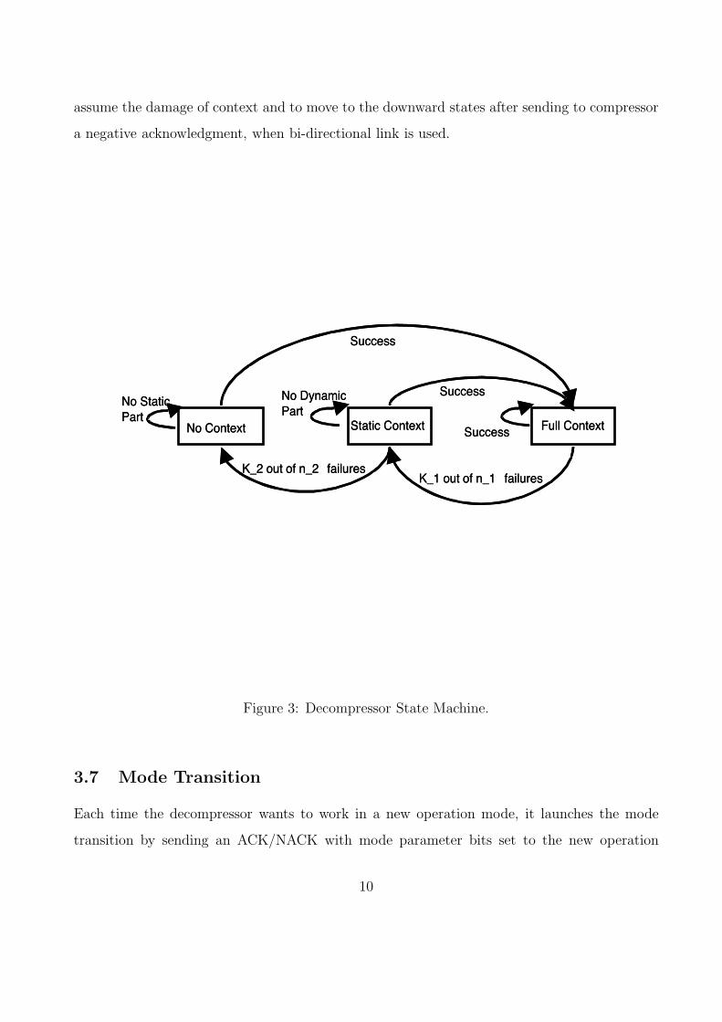
assume the damage of context and to move to the downward states after sending to compressor

a negative acknowledgment, when bi-directional link is used.

No Context Static Context Full Context

Success

Success

Success

No Static

Part

No Dynamic

Part

K_2 out of n_2 failuresK_1 out of n_1 failures

No Context Static Context Full Context

Success

Success

Success

No Static

Part

No Dynamic

Part

K_2 out of n_2 failuresK_1 out of n_1 failures

Figure 3: Decompressor State Machine.

3.7 Mode Transition

Each time the decompressor wants to work in a new operation mode, it launches the mode

transition by sending an ACK/NACK with mode parameter bits set to the new operation

10

mode. During transition, the compressor is allowed to work only in the first two compression

levels, all the packets sent contain a CRC to verify the information, each of the compressor

and the decompressor keeps two control variables: Transition and Mode and they deny any

new request for transition till current transition gets completed. If the transition variable has a

pending value, the transition mode cannot be released. To finish the transition, an ACK with

the valid sequence number and the new operation mode has to be received by the compressor,

if it is not the case, the transition variable keeps the pending value and Mode variable keeps

the old value. In addition, to initiate the transition to the R mode, the context must have

been established between the compressor and the decompressor. For the other transitions, the

decompressor can start the transition mode at any moment.

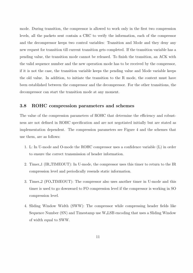
3.8 ROHC compression parameters and schemes

The value of the compression parameters of ROHC that determine the efficiency and robust-

ness are not defined in ROHC specification and are not negotiated initially but are stated as

implementation dependent. The compression parameters see Figure 4 and the schemes that

use them, are as follows:

1. L: In U-mode and O-mode the ROHC compressor uses a confidence variable (L) in order

to ensure the correct transmission of header information.

2. Timer 1 (IR TIMEOUT): In U-mode, the compressor uses this timer to return to the IR

compression level and periodically resends static information.

3. Timer 2 (FO TIMEOUT): The compressor also uses another timer in U-mode and this

timer is used to go downward to FO compression level if the compressor is working in SO

compression level.

4. Sliding Window Width (SWW): The compressor while compressing header fields like

Sequence Number (SN) and Timestamp use W LSB encoding that uses a Sliding Window

of width equal to SWW.

11

5. W LSB encoding is used to compress those header fields whose change pattern is known.

When using this encoding, the compressor sends only the least significant bits. The

decompressor uses these bits to construct the original value of the encoding fields.

6. k and n: The ROHC decompressor uses a ”k out of n” failure rule, where k is the number

of packets received with an error in the last n transmitted packets. This rule is used in the

state machine of the decompressor to assume the damage of context and move downwards

to a state after sending a negative acknowledgment to the compressor, if bi-directional

link is used. The decompressor does not assume context damage and stays in the current

state until k packets arrive with error in the last n packets. The k1, n1 values are used

to assume dynamic context damage and k2, n2 to assume static context damage.

7. MODE: There are two bits in the header format packets to define the operation mode in

which the compressor and the decompressor work. There are only three-operation modes,

U, O and R mode defined in Bormann et al. (2001).

UTRAN

Compressor Decompressor

UO-0 UO-1 UOR-2 IR-DYN IR N

Feedback

UE

SWW, L,

IR_TIMEOUT,

FO_TIMEOUT

k1, n1,

k2, n2

MODE bits

UTRAN

Compressor Decompressor

UO-0 UO-1 UOR-2 IR-DYN IR N

Feedback

UE

SWW, L,

IR_TIMEOUT,

FO_TIMEOUT

k1, n1,

k2, n2

MODE bits

Figure 4: The Compression Parameters. They are localized in the compressor, in the decom-

pressor and in the different header format packets. Note that at each end of the link both

Compressor and Decompressor are present.

4 ROHC Compression Implementation

The ROHC implementation is the development of Profile 1 (IPv6/UDP/RTP) header compres-

sion. It returns the sequence of packets sent, the average throughput, the number of CRC failed

12

packets in the ROHC implementation and the number of lost packets in the application, the

sequence number execution, the header size in each packet sent and received and the number

of each ROHC packet sent. Our experimental system consists of a video application platform

in IPv6 and a PPPoev6 based on FreeBSD4.5 with Kame. There are two computers connected

by a PPP channel. Each side of the PPP channel has a ROHC node formed by a compressor

and a decompressor entities. The ROHC compressor function needs an IP packet and a context

as input and it outputs the compressed ROHC packet. The ROHC compressor functions uses

the context space to store information regarding context flows. The receive function is called

from the decompressor function of the same side. While receiving a packet if the decompressor

recognize it to be a feedback packet then it can pass it to the compressor entity of the same

node. The ROHC decompressor function needs a ROHC packet and a context as input and

it outputs the decompressed IP packets. The ROHC decompressor uses the context space to

store and retrieve information regarding context flows. The decompressor needs to send feed-

backs depending on the operation mode of ROHC. This is currently done by using a link layer

function from PPP library. In U-mode the compressor periodically comes back to previous

compression levels and in the implementation this is done by using PPP library for PPP timer.

The platform is composed of a video application located in both nodes. Through the PPPoe,

the client receives the video header compressed packets that will be decompressed by the ROHC

decompressor in the other node. At the beginning, node A is in U-mode. No feedback is sent

by node B until the acknowledgment sent by B changes the operation mode of compressor.

The ROHC negotiation is made when the channel is open between A and B, then the NCP v6

packet is sent to node B. Then, the PPP interface starts sending the packets. The values of the

different parameters are changed before a simulation because they are not negotiated by the

actual ROHC standard. We have developed a UMTS error simulator, which generates UMTS

error traces. The error traces are first generated as random sequences based on the error levels

of the UMTS radio link (Holma and Toskala (2001)). These error traces are fed to our IPv6

ROHC Profile 1 implementation. In the graph of Figure 5, we can see the general behavior of

ROHC in every operation modes. The size of original header of IPv6/UDP/RTP is 60 bytes

shown as a dashed line in Figure 5. The solid line indicates the size of the compressed headers.

13

The compressor always starts in the U-mode and the bigger headers seen in Figure 5 are the IR

packets, which are sent periodically in the U-mode to refresh static information in the context

of the decompressor.

The mode transitions can also be seen in Figure 5 and it can be noted that while mode tran-

sition, the compressor cannot send the smallest compressed headers that are of SO compression

level. We can also see the difference between the three modes and compare their compression

efficiency. We notice the difference between O-mode and R-mode and see the increased use of

feedback channel in the later. The R-mode is interesting because the confidence system (L)

is not used as in U and O modes. The larger headers are only sent at the beginning or when

the context is lost and most of the time, SO packets are used. The performance in the uplink

is improved in R-mode because the smallest headers are used more frequently than the larger

ones. It is important to mention that Figure 5 is the evolution of the compression with small

BER and it is used only for comparing compression efficiency. When the error is small, the

O-mode performance is found better than the R-mode because downlink is used less in the

former than the latter; but the case is entirely different in a noisy link where the increased use

of the downlink in the R-mode gives better feedback and hence, better robustness. ROHC over

a radio link for IPv6 gives two types of errors. They occur in two types of situations as shown in

Figure 6. First is when an error occurs in the compressed header and the decompressor catches

it by ROHC CRC. The decompressor then drops the packet, it does not forward it to the IPv6

layer, when this happens the error is produced by ROHC and we call it ROHC loss. The other

situation is when an error occurs in the payload then the decompressor is unable to catch the

error and forwards it to the IPv6 layer. When the payload is handed to the UDP and since

for IPv6 the UDP checksum is mandatory, the error is caught and the packet is discarded, we

call it Application loss. This loss can be undesired because most sources (video, speech coders)

developed for cellular links tolerate errors in the encoded data. Such coders will want damaged

packets to be still delivered to them and will not want to enable UDP Checksum. The solution

would be the use of UDP-Lite but this implies for ROHC a new profile that has standardized

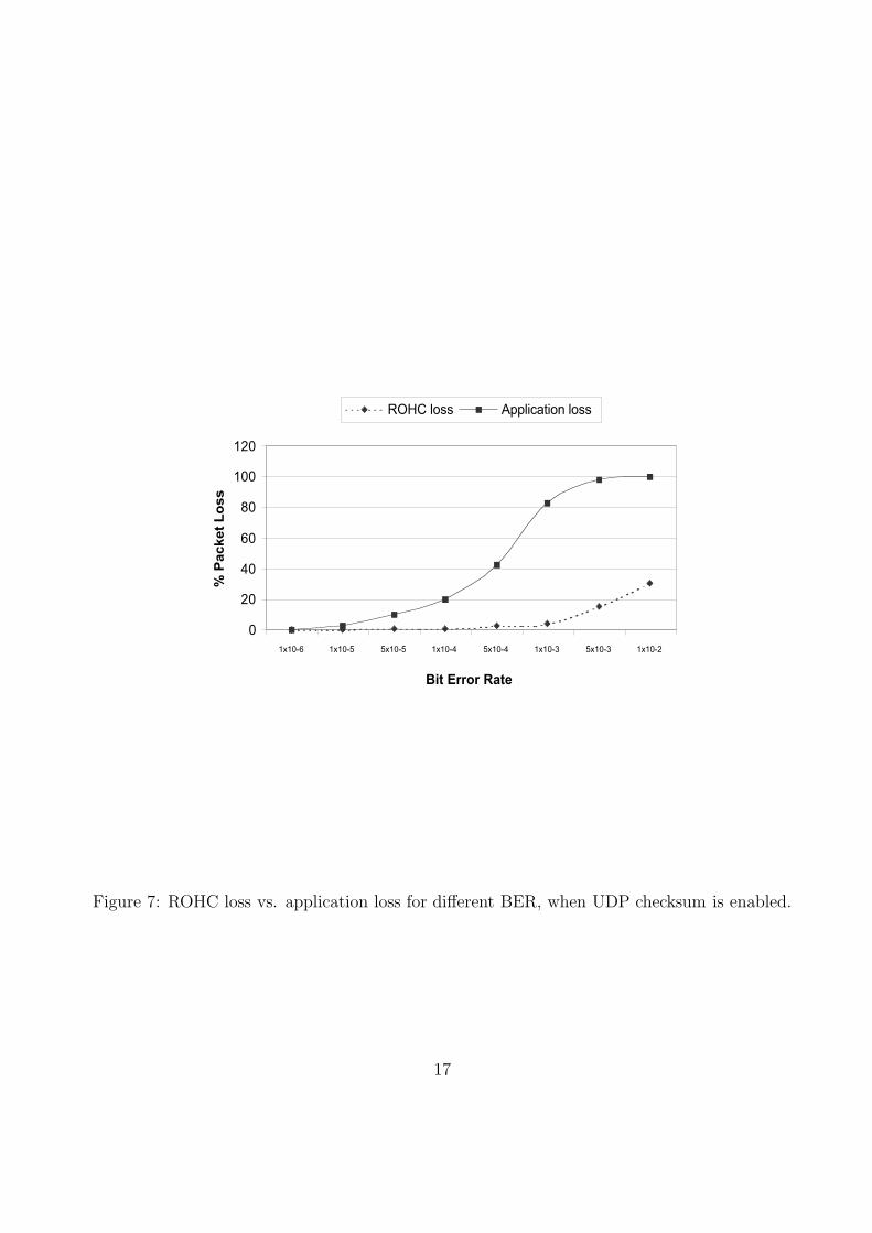
very recently in RFC 4019 (Pelletier (2005)). The performance of ROHC compression with dif-

ferent error rates is shown in Figure 7, we can see that the BER affects more often the payload

14

Number of Packets

Head

er

Siz

e(b

yte

s)

Profile 1

1

48

95

142

189

236

283

330

377

424

471

518

565

612

659

706

753

800

847

894

0

20

40

60

Transition

Acknowledgement

U-mode U-O -mode O -modeR -modeR -mode

Non Compression

1

48

95

142

189

236

283

330

377

424

471

518

565

612

659

706

753

800

847

894

U-mode U-O -mode O -modeR -modeR -mode

mode

Figure 5: ROHC compression. Illustration of Operation Modes (U, O, R), Transition Modes

and the use of feedback with small error. The ACK packets from 200 to 236 correspond to

the transition from the U-mode to the O-mode. Those from 260 to 270 and from 327 to

333 correspond to negative ACKs in the O-mode. Those from 366 to 380 correspond to the

transition from the O-mode to the R-mode. Those from 380 to 490 correspond to poositive

and negative ACKs in the R-mode. Those from 490 to 510 correspond to the transition from

the R-mode to the O-mode and so on.

15

than the header information. From Figure 7 we find that the Application loss as compared to

the ROHC loss is significant and would lead to bad performance.

Figure 6: The ROHC Architecture has two types of error.

5 Analytical Model

We consider a packet flow which may represent the transfer of a large data file from a video

streaming server to a client. The flow is composed of successive and identical cycles which

correspond to the sending of T packets, where T is called the timer. Each cycle is itself composed

of five compression phases. In each of the first four phases, L packets are sent with an increasing

compression degree. We denote by `(n) the compressed header length of a packet in the n-th

phase. The L packets of the first phase are sent with their header uncompressed, which means

that `(1) = 67 bytes. This first phase is the initialization phase of the compression process.

The L packets headers of the second, third and fourth phases are compressed to `(2) = 23

bytes, `(3) = 6 bytes, and `(4) = 5 bytes respectively. In the fifth phase, the remaining T − 4L

packets of the cycle are sent with their headers compressed to `(5) = 4 bytes. Next, a new

cycle with the same behavior begins and so on. Thus, the parameters T and L must be such

16

0

20

40

60

80

100

120

1x10-6 1x10-5 5x10-5 1x10-4 5x10-4 1x10-3 5x10-3 1x10-2

Bit Error Rate

%P

acket

Lo

ss

ROHC loss Application loss

Figure 7: ROHC loss vs. application loss for different BER, when UDP checksum is enabled.

17

that T > 4L. Their values have to be adjusted in order to satisfy performances criteria as we

shall see in the examples.

It must be noted that when the L packets headers of the first phase are all erroneously

transmitted then all the packets of the whole cycle will be lost because the protocol needs at

least one uncompressed packet, i.e. one packet of the first phase, to be transmitted correctly.

We denote by b the Bit Error Rate (BER), that is the probability that a bit is not correctly

received and by m the payload size of a packet, that is the quantity, in bits of useful data to

be transmitted (of course the header is not included in the payload). As usual in stochastic

modelling, the parameter b summarizes several features such as multipath Rayleigh fading,

residuals errors, block errors, handover, etc. At the n-th phase, n = 1, 2, 3, 4, 5, the header

length `(n), in bits, of a packet is composed of two parts: a part of this header having size c(n),

which may be corrected after some faults with probability p, using error correction heuristics

and the rest of size `(n) − c(n) which cannot be corrected.

The values of c(n) in bits are c(1) = 80, c(2) = 80, c(3) = 12, c(4) = 10 and c(5) = 4.

and we suppose that the events associated with the error transmissions are independent. The

probability pn of sending correctly a packet in the phase n is thus given, for 1 ≤ n ≤ 5, by

pn = (1 − b)m+`(n) + (1 − b)m+`(n)−c(n)(1 − (1 − b)c(n))p.

The first term corresponds to the fact that the whole packet has been sent correctly and the

second term corresponds to the fact that at least one bit of the part of length c(n) has failed

but it has been successfully corrected.

After the transmission of a packet, we will say that we had a success if the packet arrived

correctly (either because there was no error, or because errors were all corrected), a failure if

the transmission failed but if, in the same cycle, not all the transmissions failed, and a total

failure if the transmission failed as well as all the previous transmissions in the cycle. Let us

code 1, 2 and 3 these three possible transmission results, and let us also call them levels. We

will define a stochastic process {Xn, n ≥ 1}, where Xn = (i, l) if after transmitting the nth

packet the result is l ∈ {1, 2, 3}, i being the rank of the packet in its cycle, that is, i = [(n− 1)

mod T ] + 1. It is immediate to see that {Xn} is a discrete time homogeneous Markov chain

18

whose associated transition graph is depicted in Figure 8 for the case L = 3 and T = 14. The

states of the first level represented using circles are denoted by (i, 1), for i = 1, . . . , T , from

left to right. The states of the second level represented using squares are denoted by (i, 2), for

i = 2, . . . , T (state (1, 2) is not feasible), from left to right and the states of the third level in

diamond shape are denoted by (i, 3), for i = 1, . . . , T , from left to right.

Since we are interested in the stationary behavior of the protocol, we denote by X the

stationary version of the Markov chain {Xn}. This version exists since the Markov chain is

finite and irreducible.

The transition from state (1, 1) to state (2, 1) corresponds to the successful transmission of

the second packet of the current cycle, so its probability is equal to p1, when L > 1. In the

same way, a transition from state (i− 1, 1) to state (i, 1) or from state (i− 1, 2) to state (i, 1),

for i = 2, . . . , T , corresponds to the successful transmission of the i-th packet of the current

cycle, so its probability is equal to pn if states (i, 1) or (i − 1, 2) belongs to the n-th phase of

the cycle. The transition probability from state (T, 1) to state (1, 1) or from state (T, 2) to

state (1, 1) is thus equal p1 and means the successful transmission of the first packet of the next

cycle.

The transition from state (1, 1) to state (2, 2) corresponds to the unsuccessful transmission

of the second packet of the current cycle, so its probability is equal to 1 − p1, when L > 1. In

the same way, a transition from state (i − 1, 1) to state (i, 2) or from state (i − 1, 2) to state

(i, 2), for i = 3, . . . , T , corresponds to the unsuccessful transmission of the i-th packet of the

current cycle, so its probability is equal to 1 − pn if state (i − 1, 1) belongs to the n-th phase

of the cycle. The transition probability from state (T, 1) to state (1, 3) or from state (T, 2) to

state (1, 3) is thus equal 1 − p1 and means the unsuccessful transmission of the first packet of

the next cycle. A new cycle then begins with the same probabilistic behavior.

The states of the third level (diamond shape) that we denoted by (i, 3), for i = 1, . . . , T ,

from the left to the right are used to represent the case where the L packets headers of the first

phase are all erroneously transmitted which leads to the lost of all the packets of the whole

cycle.

The state (1, 3) of a current cycle is reached when the first packet of this cycle is unsuc-

19

cessfully transmitted, i.e. from states (T, 1), (T, 2) or (T, 3) with the same probability 1 − p1.

Next, a transition from state (i − 1, 3) to state (i, 3), for i = 2, . . . , L, corresponds to the un-

successful transmission of the i-th packet, so its probability is equal to 1−p1. In the same way,

a transition from state (i − 1, 3) to state (i, 1), for i = 2, . . . , L, corresponds to the successful

transmission of the i-th packet, so its probability is equal to p1. When the process is in state

(L, 3), this means that the L first packets of the cycle have been unsuccessfully transmitted, so

the transition probability from state (i, 3) to state (T, 3), for i = L, . . . , T , is equal to 1.

�� � � �� �� � � �� �� � � ��

�� � � � � � �� � � � � � �� � � ��� � � � � �

Figure 8: The Markov chain.

20

We partition the state space in a vertical way (see Figure 8) into T subsets as follows. For

i = 1, . . . , T , we introduce the subset of states Si defined by

S1 = {(1, 1), (1, 3)} and Si = {(i, 1), (i, 2), (i, 3)} for i = 2, . . . , T.

Using this partition, the transition probability matrix P of the Markov chain {Xn} is given

by the submatrices Pi,j containing the transition probabilities form states of Si to states of Sj.

The non-zero submatrices of matrix P are given by

Pi,i+1 =

A for i = 1

B1 for 2 ≤ i ≤ L − 1

B2 for L ≤ i ≤ 2L − 1

B3 for 2L ≤ i ≤ 3L − 1

B4 for 3L ≤ i ≤ 4L − 1

B5 for 4L ≤ i ≤ T − 1

and PT,1 = C,

where the matrices A, Bn and C are defined by

A =

p1 1 − p1 0

p1 0 1 − p1

; B1 =

p1 1 − p1 0

p1 1 − p1 0

p1 0 1 − p1

;

Bn =

pn 1 − pn 0

pn 1 − pn 0

0 0 1

, for 2 ≤ n ≤ 5 and C =

p1 1 − p1

p1 1 − p1

p1 1 − p1

.

21

For example, in the case depicted in Figure 8, where L = 3 and T = 14, we have

P =

0 A 0 0 0 0 0 0 0 0 0 0 0 0

0 0 B1 0 0 0 0 0 0 0 0 0 0 0

0 0 0 B2 0 0 0 0 0 0 0 0 0 0

0 0 0 0 B2 0 0 0 0 0 0 0 0 0

0 0 0 0 0 B2 0 0 0 0 0 0 0 0

0 0 0 0 0 0 B3 0 0 0 0 0 0 0

0 0 0 0 0 0 0 B3 0 0 0 0 0 0

0 0 0 0 0 0 0 0 B3 0 0 0 0 0

0 0 0 0 0 0 0 0 0 B4 0 0 0 0

0 0 0 0 0 0 0 0 0 0 B4 0 0 0

0 0 0 0 0 0 0 0 0 0 0 B4 0 0

0 0 0 0 0 0 0 0 0 0 0 0 B5 0

0 0 0 0 0 0 0 0 0 0 0 0 0 B5

C 0 0 0 0 0 0 0 0 0 0 0 0 0

.

We denote by π the stationary distribution of the Markov chain. We thus have

π = πP and π1 = 1, (1)

where 1 denotes the column vector with all entries equal to 1, its dimension being specified by

the context where it is used. We decompose the vector π using the partition of the state space

defined by the subsets Si. So, for i = 1, . . . , T , we define the subvectors πi such that

π = (π1, . . . , πL, πL+1, . . . , π2L, π2L+1, . . . , π3L, π3L+1, . . . , π4L, π4L+1, . . . , πT ) ,

where πi is the row subvector of vector π containing the entries corresponding to subset Si,

that is

π1 = (π(1, 1), π(1, 3)) and πi = (π(i, 1), π(i, 2), π(i, 3)) for i = 2, . . . , T.

The linear system (1) then becomes in terms of the subvectors πi and submatrices A, Bn, for

n = 1, 2, 3, 4, 5 and C

22

π1 = πT C

π2 = π1A

π3 = π2B1

......

...

πL = πL−1B1

;

πL+1 = πLB2

πL+2 = πL+1B2

πL+3 = πL+2B2

...

π2L = π2L−1B2

;

π2L+1 = π2LB3

π2L+2 = π2L+1B3

π2L+3 = π2L+2B3

...

π3L = π3L−1B3

;

π3L+1 = π3LB4

π3L+2 = π3L+1B4

π3L+3 = π3L+2B4

...

π4L = π4L−1B4

;

π4L+1 = π4LB5

π4L+2 = π4L+1B5

π4L+3 = π4L+2B5

...

πT = πT−1B5

(2)

The submatrices A, Bn, for n = 1, 2, 3, 4, 5 and C are stochastic, so by multiplying the equations

of linear system (2) by the colum vector 1 on the right, we get

π11 = π21 = · · · = πT1,

which leads, by using the equation π1 = 1, to

πi1 =1

T, for 1 ≤ i ≤ T.

It is now very easy to solve system (2). The first set of equations gives us

π1 =1

T(p1, 1 − p1) .

For 2 ≤ i ≤ L,

πi =1

T

(p1, 1 − p1 − (1 − p1)

i, (1 − p1)i).

The four other sets of equations give us:

For L + 1 ≤ i ≤ 2L,

πi =1

T

(p2(1 − (1 − p1)

L), (1 − p2)(1 − (1 − p1)L), (1 − p1)

L).

23

For 2L + 1 ≤ i ≤ 3L

πi =1

T

(p3(1 − (1 − p1)

L), (1 − p3)(1 − (1 − p1)L), (1 − p1)

L).

For 3L + 1 ≤ i ≤ 4L

πi =1

T

(p4(1 − (1 − p1)

L), (1 − p4)(1 − (1 − p1)L), (1 − p1)

L).

For 4L + 1 ≤ i ≤ T

πi =1

T

(p5(1 − (1 − p1)

L), (1 − p5)(1 − (1 − p1)L), (1 − p1)

L).

We denote by phit the probability that the transmission of all packets is correct. It is thus

the probability for the Markov chain to be in one of the states (i, 1), for i = 1, . . . , T . This

probability is also the sum of the first entries of all subvectors πi. Thus we have

phit =T∑

i=1

π(i, 1) =T∑

i=1

πi(1),

which leads to

phit =1

T

[Lp1 +

(L(p2 + p3 + p4) + (T − 4L)p5

)(1 − (1 − p1)

L)]

. (3)

6 Numerical Results

In order to validate our analytical model we compared its results with the results obtained

by the implementation and we observed that the accuracy is quite good. Since we focused on

ROHC effects, we made our experiments without payloads, i. e. with m = 0. The values

of the other input parameters are the following: the timer has been fixed to T = 800 and

the probability p associated with the error corrections is p = 0. To illustrate this, Figure 9

represents the stationary packet loss probability ploss, which is equal to 1−phit, as a function of

the phases length L for different values of the bit error rate b. Concerning the latter, we focus

in realistic and common transmission situations where the bit error rate is small, say less than

or equal to 10−4. The behaviour of the model for this bit error rate is shown at the bottom

24

of Figure 9. Recall that the goal is performance evaluation, that is, the analysis of average

behaviour under usual conditions: this means that we avoid in our models and experiences

extreme situations. Figure 9 thus shows that the model is quite accurate when b = 10−4.

We also show, however, what happens for higher (and less frequent) values of b; the goal is

to illustrate that accuracy improves as b decreases, and also that the global behaviour of the

model remains reasonably close to the experimental values even if too many bits are lost. It is

worth noting that the model has been validated for several values of the parameter T .

0.001

0.01

0.1

1

2 3 4 5 6 7 8 9 10

Loss

proba

bility

L

b = 0.005

b = 0.001

b = 0.0001

modelimplementation

Figure 9: Validating the analytical model.

Using our model, we can compute the stationary packet loss probability for several parameter

values.

Note that from relation (3), when L is large, the loss probability ploss, is approximatively

proportional to the ratio L/T . More formally, when L −→ ∞ and T −→ ∞ and L/T −→ r,

with r < 1/4, we have

ploss −→ r(p1 + p2 + p3 + p4) + (1 − 4r)p5.

Figure 10 shows the behavior of the packet loss probability for b = 10−4. This figure allows

us to choose the parameters b, L and T so that the loss probability is less than or equal to a

25

given value. This figure shows for instance that the global minimum loss probability is reached

when L = 4 and T = 800 where we have ploss = 0.0035.

0

0.005

0.01

0.015

0.02

2 3 4 5 6 7 8 9 10

Loss

proba

bility

L

Figure 10: For b = 0.0001 from top to bottom: T = 50, T = 100, T = 200, T = 300, T = 600,

T = 800.

7 Conclusion

The ROHC description of this paper gives an overview of the protocol complexity and the num-

ber of different parameters that must be set. We developed an analytical model of this protocol

based only on the first compressor profile with the unidirectional mode. This mode represents

the most common use of ROHC in low bandwidth links. We have shown that this model,

described by a Markov chain, is quite accurate and, thus, that the analytical results it provides

constitute a step towards establishing relations between configuration parameters and the error

rate. This will help the configuration process itself, will contribute to the auto-configuration of

the link layer and will allow to optimize the performance of the header compression algorithm.

26

References

Boggia, G., Camarda, P. and Squeo, V.G. (2002). ROHC+: A New Header Compression

Scheme for TCP Streams in 3G Wireless Systems. In IEEE ICC, 3271–3278.

Bormann, C., Burmeister, C., Degermark, M., Fukushima, H., Hannu, H., Jonsson, L.-E.,

Hakenberg, R., Koren, T., Le, K., Liu, Z., Martensson, A., Miyazaki, A., Svanbro, K., Wiebke,

T., Yoshimura, T., and Zheng, H. (2001). Robust Header Compression (ROHC): Framework

and four profiles: RTP, UDP, ESP and Uncompressed. RFC 3095, July.

Casner, S., and Jacobson, V. (1999). Compressing IP/UDP/RTP Headers for Low-Speed

Serial Links. RFC 2508, February.

Degermark, M., Nordgren, B., and Pink, S. (1999). IP Header Compression. RFC 2507,

February.

Farber, D.J., and Delp, G.S. (1994). A Thinwire Protocol for connecting personal computers

to the INTERNET. RFC 914, September.

Giovanardi, A., Mazzini, G., Rossi, M., and Zorzi, M. (2000). Improved Header Compression

for TCP/IP over Wireless Links. IEEE Electronics Letters, 1958–1960, November.

Holma, H., and Toskala, A. (2001). WCDMA for UMTS. John Wiley and Sons.

Jacobson, V. (1990). Compressing TCP/IP Headers for Low-Speed Serial Links. RFC 1144,

February.

Jonsson,L.-E. (2002). The ROHC Architecture. INTERNET-DRAFT.

Jonsson, L.-E., Degermark, M., Hannu, H., and Svanbro, K. (1999). RObust Checksum-based

header COmpression (ROCCO) version 06. INTERNET-DRAFT, June.

Le, K., Clanton, C., Liu, Z., and Zheng, H. (2000). ACE: A Robust and Efficient IP/UDP/RTP

Header Compression Sheme. INTERNET-DRAFT, March.

27

Liao, H., Zhang, Q., Zhu, W., Zhang, Y.-Q., Price, R., Hancok, R., McCann, S., West,

M.A., Surtees, A., and Ollis, P. (2001). TCP-Aware RObust Header Compression (TAROC).

INTERNET-DRAFT, November.

Miyazaki, A., Fukushima, H., Wiebke, T., Hakenberg, R., and Burmeister, C. (2000). Robust

Header Compression using Keyword-Packets. INTERNET-DRAFT, May.

Pelletier, G. (2005). RObust Header Compression (ROHC): Profiles for User Datagram Pro-

tocol (UDP) Lite. RFC 4019, April.

Perkins, S., and Mutka, M.W. (1997). Dependency Removal for Transport Protocol Header

Compression Over Noisy Channels. In IEEE ICC, 1025–1029, 1997.

Price, R., McCann, S., Surtees, A., Ollis, P., and M. West. (2002). Framework for EPIC-LITE.

INTERNET-DRAFT, February.

28