Perfect Competition —Definition

What is the essence of perfect competition?

All agents in the market take the relevant price for this market asgiven.

That is, all agents assume that their behaviour will not affect themarket price. Moreover, they assume that they can buy or sell as muchas they like at the market price.

By agents we mean both Firms and Consumers.

Notice that often a firm has market power:

sometimes can affect the price (a large firm in a market)sometimes it is the only firm in the market (monopoly)

But also a consumer sometimes has market power

Think of the government as a consumer of weapons.

() October 10, 2012 1 / 20

Perfect Competition —Environment

What makes a market behave perfectly competitive?

Many atomistic buyers and producers

Homogenous good

Perfect information (consumers and firms).

Free entry and exit.

Perfectly divisible output.

No transaction costs.

() October 10, 2012 2 / 20

Demand Side

We assume that the aggregate demand curve for a good isdownward-sloping

q = D(p), where D ′(p) < 0.

Often it is more convenient to work with the inverse demand function:

p = P(q) where P ′(q) < 0.

How can we derive this function?

() October 10, 2012 3 / 20

Derivation of Demand Curve

DEMAND FOR PIZZA

First slice —what would be the maximum you would pay for one sliceof pizza?

Say, £ 3.

How about the second slice? (this is after you had your first slice)

Say, £ 1.5 (certainly less than for the first slice).

And for the third slice? (this is after you had your second slice)

Say, £ 0.2 (certainly less than for the second slice).

() October 10, 2012 4 / 20

Derivation of Demand Curve

DEMAND FOR PIZZA

() October 10, 2012 5 / 20

Consumers Welfare

From the demand function, we can first derive the total utilityobtained from x units of pizza.

More importantly, knowing the market price, we can obtain theconsumer surplus

This is the utility net of the monetary cost to buy the pizza

Consumer surplus from x units of pizza.

if buying one slice: 3− 1 = 2if buying two slices: (3+ 1.5)− 2× 1 = 2.5if buying three slices: (3+ 1.5+ 0.2)− 3× 1 = 1.7

Demanded quantity of pizza if p = 1: 2 slices.

What if p = 0.19?

() October 10, 2012 6 / 20

Supply Side —Cost Functions

1 Fixed cost (FC): The cost that does not depend on the amount ofoutput produced

2 Variable cost (VC): The cost that rises with output (and equals zeroif no output is produced)

3 Total cost (TC): TC (q) = FC + VC (q).

4 Average or unit cost (AC): AC (q) =TC (q)q

.

5 Marginal cost (MC): the cost of one (infinitesimal) additional unit.

MC (q) =∂TC (q)

∂q.

If working with discrete quantities: MC (q) = TC (q + 1)− TC (q)

() October 10, 2012 7 / 20

Supply Side —Costs

The MC function crosses the AC cost function at the minimumaverage cost level... Why?

() October 10, 2012 8 / 20

Equality of minimum AC and MC —mathematical proof

Let qmin denote the output that minimizes AC (q). Then:

∂AC (qmin)∂q

= 0. (1)

Recalling that AC (q) = TC (q)/q, then it follows that:

∂AC (q)∂q

=

∂TC (q)∂q

q − TC (q)

q2. (2)

Bearing in mind (1), the numerator in (2) must thus equal zero whenq = qmin. That is,

∂TC (qmin)∂q

qmin = TC (qmin).

But, MC (q) = ∂TC (q)/∂q and AC (q) = TC (q)/q, then:

MC (qmin) = AC (qmin).

() October 10, 2012 9 / 20

Equality of minimum AC and MC —mathematical proof

Let qmin denote the output that minimizes AC (q). Then:

∂AC (qmin)∂q

= 0. (1)

Recalling that AC (q) = TC (q)/q, then it follows that:

∂AC (q)∂q

=

∂TC (q)∂q

q − TC (q)

q2. (2)

Bearing in mind (1), the numerator in (2) must thus equal zero whenq = qmin. That is,

∂TC (qmin)∂q

qmin = TC (qmin).

But, MC (q) = ∂TC (q)/∂q and AC (q) = TC (q)/q, then:

MC (qmin) = AC (qmin).

() October 10, 2012 9 / 20

Equality of minimum AC and MC —mathematical proof

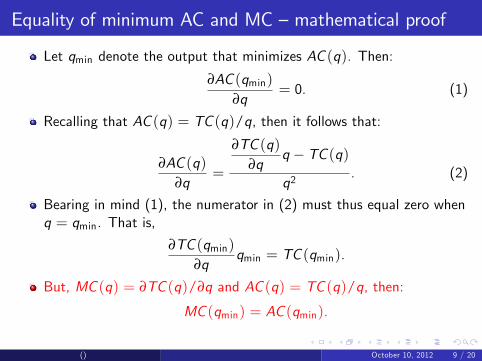
Let qmin denote the output that minimizes AC (q). Then:

∂AC (qmin)∂q

= 0. (1)

Recalling that AC (q) = TC (q)/q, then it follows that:

∂AC (q)∂q

=

∂TC (q)∂q

q − TC (q)

q2. (2)

Bearing in mind (1), the numerator in (2) must thus equal zero whenq = qmin. That is,

∂TC (qmin)∂q

qmin = TC (qmin).

But, MC (q) = ∂TC (q)/∂q and AC (q) = TC (q)/q, then:

MC (qmin) = AC (qmin).

() October 10, 2012 9 / 20

Equality of minimum AC and MC —mathematical proof

Let qmin denote the output that minimizes AC (q). Then:

∂AC (qmin)∂q

= 0. (1)

Recalling that AC (q) = TC (q)/q, then it follows that:

∂AC (q)∂q

=

∂TC (q)∂q

q − TC (q)

q2. (2)

Bearing in mind (1), the numerator in (2) must thus equal zero whenq = qmin. That is,

∂TC (qmin)∂q

qmin = TC (qmin).

But, MC (q) = ∂TC (q)/∂q and AC (q) = TC (q)/q, then:

MC (qmin) = AC (qmin).

() October 10, 2012 9 / 20

Fixed and Variable Costs —examples

Consider a steel producer

Fixed costs

RentLoan paymentsMaintenance

Variable costs

Intermediate inputs: water, electricity, fuel, iron...Labour costTaxes

() October 10, 2012 10 / 20

Fixed and Variable Costs —time horizon

Fixed costs are mostly related to the size of the plant

by varying the size of the plant, we may change the rent, the level ofmaintenance, the size of the loan required to set up the plant...

From that perspective fixed costs are only ‘fixed’in the short run

What makes a cost fixed or variable is a related to the time horizon ofthe analysis

Then, in the long run all costs are variable.

() October 10, 2012 11 / 20

Fixed and Variable Costs —time horizon

Fixed costs are mostly related to the size of the plant

by varying the size of the plant, we may change the rent, the level ofmaintenance, the size of the loan required to set up the plant...

From that perspective fixed costs are only ‘fixed’in the short run

What makes a cost fixed or variable is a related to the time horizon ofthe analysis

Then, in the long run all costs are variable.

() October 10, 2012 11 / 20

Fixed and Variable Costs —time horizon

Fixed costs are mostly related to the size of the plant

by varying the size of the plant, we may change the rent, the level ofmaintenance, the size of the loan required to set up the plant...

From that perspective fixed costs are only ‘fixed’in the short run

What makes a cost fixed or variable is a related to the time horizon ofthe analysis

Then, in the long run all costs are variable.

() October 10, 2012 11 / 20

Fixed and Variable Costs —time horizon

Fixed costs are mostly related to the size of the plant

by varying the size of the plant, we may change the rent, the level ofmaintenance, the size of the loan required to set up the plant...

From that perspective fixed costs are only ‘fixed’in the short run

What makes a cost fixed or variable is a related to the time horizon ofthe analysis

Then, in the long run all costs are variable.

() October 10, 2012 11 / 20

Fixed and Variable Costs —time horizon

Fixed costs are mostly related to the size of the plant

by varying the size of the plant, we may change the rent, the level ofmaintenance, the size of the loan required to set up the plant...

From that perspective fixed costs are only ‘fixed’in the short run

What makes a cost fixed or variable is a related to the time horizon ofthe analysis

Then, in the long run all costs are variable.

() October 10, 2012 11 / 20

Firm’s Optimisation Problem

Producer solves

maxq

: Π(q) = P(q)q − VC (q)− FC

First Order Condition:

∂Π(q)∂q

= 0 ⇔ P(q) +∂P(q)

∂q−MC (q) = 0

under perfect competition: P(q) = p, then

∂P(q)∂q

= 0

Competitive firm sets q∗ such that:

p = MC (q∗)

() October 10, 2012 12 / 20

Firm’s Optimisation Problem

Producer solves

maxq

: Π(q) = P(q)q − VC (q)− FC

First Order Condition:

∂Π(q)∂q

= 0 ⇔ P(q) +∂P(q)

∂q−MC (q) = 0

under perfect competition: P(q) = p, then

∂P(q)∂q

= 0

Competitive firm sets q∗ such that:

p = MC (q∗)

() October 10, 2012 12 / 20

Firm’s Optimisation Problem

Producer solves

maxq

: Π(q) = P(q)q − VC (q)− FC

First Order Condition:

∂Π(q)∂q

= 0 ⇔ P(q) +∂P(q)

∂q−MC (q) = 0

under perfect competition: P(q) = p, then

∂P(q)∂q

= 0

Competitive firm sets q∗ such that:

p = MC (q∗)

() October 10, 2012 12 / 20

Firm’s Optimisation Problem —Firm’s supply curve

But, is the condition p = MC (q∗) enough?

Actually, it may not be enough...If p < VC (q)

q , then the firm prefers to set q∗ = 0... Why?

So, the firm’s supply curve can be plotted as

() October 10, 2012 13 / 20

Firm’s Optimisation Problem —Firm’s supply curve

But, is the condition p = MC (q∗) enough?Actually, it may not be enough...

If p < VC (q)q , then the firm prefers to set q∗ = 0... Why?

So, the firm’s supply curve can be plotted as

() October 10, 2012 13 / 20

Firm’s Optimisation Problem —Firm’s supply curve

But, is the condition p = MC (q∗) enough?Actually, it may not be enough...If p < VC (q)

q , then the firm prefers to set q∗ = 0... Why?

So, the firm’s supply curve can be plotted as

() October 10, 2012 13 / 20

Firm’s Optimisation Problem —Firm’s supply curve

But, is the condition p = MC (q∗) enough?Actually, it may not be enough...If p < VC (q)

q , then the firm prefers to set q∗ = 0... Why?

So, the firm’s supply curve can be plotted as

() October 10, 2012 13 / 20

Aggregate supply curve

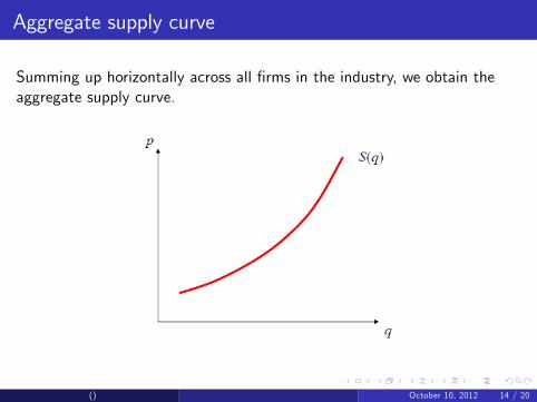
Summing up horizontally across all firms in the industry, we obtain theaggregate supply curve.

() October 10, 2012 14 / 20

Equilibrium

The perfect competition equilibrium lies at the intersection of demand andsupply curves:

() October 10, 2012 15 / 20

Equilibrium: short vs. long run

In the short run, the number of firms is fixed...

Hence, firms may make positive profits in the short run.

But a feature of perfect competition is: free entry

With free entry, positive profits must attract new firms to enter themarket.

In the long run new firms must enter so long as profits remainpositive.

Hence, in the long run profits must be zero when there is perfectcompetition.

() October 10, 2012 16 / 20

Equilibrium: short vs. long run

In the short run, the number of firms is fixed...

Hence, firms may make positive profits in the short run.

But a feature of perfect competition is: free entry

With free entry, positive profits must attract new firms to enter themarket.

In the long run new firms must enter so long as profits remainpositive.

Hence, in the long run profits must be zero when there is perfectcompetition.

() October 10, 2012 16 / 20

Equilibrium: short vs. long run

In the short run, the number of firms is fixed...

Hence, firms may make positive profits in the short run.

But a feature of perfect competition is: free entry

With free entry, positive profits must attract new firms to enter themarket.

In the long run new firms must enter so long as profits remainpositive.

Hence, in the long run profits must be zero when there is perfectcompetition.

() October 10, 2012 16 / 20

Equilibrium: short vs. long run

In the short run, the number of firms is fixed...

Hence, firms may make positive profits in the short run.

But a feature of perfect competition is: free entry

With free entry, positive profits must attract new firms to enter themarket.

In the long run new firms must enter so long as profits remainpositive.

Hence, in the long run profits must be zero when there is perfectcompetition.

() October 10, 2012 16 / 20

Equilibrium: short vs. long run

In the short run, the number of firms is fixed...

Hence, firms may make positive profits in the short run.

But a feature of perfect competition is: free entry

With free entry, positive profits must attract new firms to enter themarket.

In the long run new firms must enter so long as profits remainpositive.

Hence, in the long run profits must be zero when there is perfectcompetition.

() October 10, 2012 16 / 20

Equilibrium: short vs. long run

In the short run, the number of firms is fixed...

Hence, firms may make positive profits in the short run.

But a feature of perfect competition is: free entry

With free entry, positive profits must attract new firms to enter themarket.

In the long run new firms must enter so long as profits remainpositive.

Hence, in the long run profits must be zero when there is perfectcompetition.

() October 10, 2012 16 / 20

EquilibriumFrom the short to long run

() October 10, 2012 17 / 20

Long-run Competitive Equilibrium —Productive Effi ciency

1 Under perfect competition, firms set production to equalise:

MC (q∗) = p.

2 At the minimum level of the average cost function, we have:

MC (qmin) = AC (qmin).

3 In the long run competitive firms must make zero profits, hence:

AC (q∗) = p

4 Therefore, in the long run:

p = MC (qmin) = AC (qmin).

In the long run, perfect competition ensures productive effi ciency

Firms produce at a point in which they minimise their average costs.

() October 10, 2012 18 / 20

Competitive Equilibrium —Pareto Effi ciency

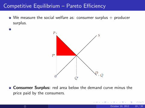
We measure the social welfare as: consumer surplus + producersurplus.

Consumer Surplus: red area below the demand curve minus theprice paid by the consumers.

() October 10, 2012 19 / 20

Competitive Equilibrium —Pareto Effi ciency

We measure the social welfare as: consumer surplus + producersurplus.

Consumer Surplus: red area below the demand curve minus theprice paid by the consumers.

() October 10, 2012 19 / 20

Competitive Equilibrium —Pareto Effi ciency

We measure the social welfare as: consumer surplus + producersurplus.

Consumer Surplus: red area below the demand curve minus theprice paid by the consumers.

() October 10, 2012 19 / 20

Competitive Equilibrium —Pareto Effi ciency

We measure the social welfare as: consumer surplus + producersurplus.

Consumer Surplus: red area below the demand curve minus theprice paid by the consumers.Producer Surplus: blue area... It equals firms’profits —why?

() October 10, 2012 20 / 20