percolazione per insiemi di livello del gaussian free eld

Universita degli Studi di Padova

Dipartimento di Matematica

“Tullio Levi-Civita”

Corso di Laurea Magistrale in Matematica

Percolazione per insiemi di livellodel Gaussian free field

Relatori:Prof. Giambattista Giacomin

Universite Paris Diderot

Prof. Paolo Dai Pra

Laureando:1130557

Jacopo Borga23 Febbraio 2018

Introduction

Existence of phase transition for the level-set percolation for the discreteGaussian free field on Zd (DGFF) is a problem that received much attentionin the past year, in particular it was studied in the 80’s by J. Bricmont, J.L.Lebowitz and C. Maes (see [3]). They showed that in three dimension theDGFF has a nontrivial percolation behavior: sites on which ϕx ≥ h percolateif and only if h < h∗ with 0 ≤ h∗ <∞. Moreover, they generalized the lowerbound for h∗ in any dimension d ≥ 3, i.e. h∗(d) ≥ 0, but they were not ableto extend the proof of existence of a non trivial transition for any d ≥ 4.Recently P.-F. Rodriguez and A.-S. Sznitman (see [11]) proved that h∗(d)is finite for all d ≥ 3 as a corollary of a more general result concerningthe stretched exponential decay of the connectivity function when h > h∗∗,where h∗∗ is a second critical parameter that satisfied h∗∗ ≥ h∗. In thisthesis we tried to get acquainted with some of the techniques developedin the domain, notably to control the large excursions of these fields andto understand the entropic repulsion phenomena, and to comprehend theresults on level set percolation in dimension three and larger. In particular,the main goal is to present the two works of Bricmont, Lebowitz and Maesand of Rodriguez and Sznitman. Finally, in the last two chapters we alsopresent a new and original (but incomplete) generalization of the proof (dueto J. Bricmont, J.L. Lebowitz and C. Maes ) of the existence of a non trivialphase transition to any d ≥ 3.

5

6

Introduzione

L’esistenza di una transione di fase per gli insiemi di livello del GaussianFree Field discreto in Zd (DGFF) e un problema che ha ricevuto molta at-tenzione negli anni passati, in particolar modo e stato studiato intorno aglianni ’80 da J. Bricmont, J.L. Lebowitz and C. Maes (vedi [3]). In questoarticolo dimostrarono che il DGFF in dimensione 3 presenta una transizionedi fase non triviale: i siti nei quali ϕx ≥ h percolano se e solo se h < h∗per 0 ≤ h∗ < ∞. Inoltre generalizzarono il bound inferiore per h∗ in ognidimensione d ≥ 3, cioe h∗(d) ≥ 0, ma non furono in grado di estendere ladimostrazione per l’esistenza di una transizione di fase non triviale ad ognid ≥ 4. Recentemente P.-F. Rodriguez e A.-S. Sznitman (vedi [11]) hannodimostrato che h∗(d) e finito per ogni dimonsione d ≥ 3 come corollario diun risultato piu generale riguardante il semi-decadimento esponenziale dellafunzione di connettivita quando h ≥ h∗∗, dove h∗∗ e un secondo parametroche soddisfa h∗∗ ≥ h∗. In questa tesi l’autore ha cercato di prendere famil-iarita con alcune tecniche sviluppate in questo dominio, in particolar modoa controllare le grandi escursioni di questi campi, capire il fenomeno di re-pulsione entropica e comprendere i risultati riguardanti la percolazione perinsiemi di livello in dimensione tre o maggiore. In particolare l’obbiettivoprincipale e quello di presentare i due lavori di Bricmont, Lebowitz e Maes edi Rodriguez e Sznitman. Infine, negli ultimi due capitoli, presenteremo unanuova ed originale (ma incompleta) generalizzazione della dimostrazione (diBricmont, Lebowitz e Maes) dell’ esistenza di una transizione di fase ad ognid ≥ 3.

Ringraziamenti

Vorrei ringraziare innanzitutto il Prof. Giambattista Giacomin per avermipermesso di realizzare questo lavoro nel periodo trascorso a Parigi, ma so-prattutto per avermi trasmesso tutta la sua passione per la Matematica.Un altro grandissimo ringraziamento va al Prof. Paolo Dai Pra per avermiseguito e sostenuto in tutti questi anni di studi.

Contents

Notation 9

1 The DGFF 111.1 The costruction of the model . . . . . . . . . . . . . . . . . . 111.2 Some heuristic interpretations . . . . . . . . . . . . . . . . . . 121.3 The random walk rappresentation for the massless model . . 13

1.3.1 Harmonic functions and the Discrete Green Identities 131.3.2 The random walk representation . . . . . . . . . . . . 16

1.4 The infinite volume extension . . . . . . . . . . . . . . . . . . 181.5 The Gibbs-Markov property. . . . . . . . . . . . . . . . . . . 20

2 Some useful general tools 252.1 Extended version for non-negative increasing functions of the

Markov’s inequality . . . . . . . . . . . . . . . . . . . . . . . . 252.2 BTIS-inequality . . . . . . . . . . . . . . . . . . . . . . . . . . 25

3 Some useful tools for the DGFF 313.1 Maximum for the Lattice Gaussian Free Field . . . . . . . . . 313.2 Asymptotics for the Green function . . . . . . . . . . . . . . . 333.3 Potential theory . . . . . . . . . . . . . . . . . . . . . . . . . 333.4 Recurrent and transient sets: The Wiener’s Test . . . . . . . 343.5 Notation for the DGFF . . . . . . . . . . . . . . . . . . . . . 343.6 Density and uniqueness for the infinite cluster . . . . . . . . . 35

4 The two main results 394.1 Purpose of the thesis . . . . . . . . . . . . . . . . . . . . . . . 394.2 The proof of J. Bricmont, J.L. Lebowitz and C. Maes . . . . 39

4.2.1 Definitions and notation . . . . . . . . . . . . . . . . . 404.2.2 The technical lemmas . . . . . . . . . . . . . . . . . . 414.2.3 Conclusion of the proof of the Theorem . . . . . . . . 43

4.3 The proof of P.-F. Rodriguez and A.-S. Sznitman . . . . . . . 434.3.1 Renormalization scheme . . . . . . . . . . . . . . . . . 444.3.2 Crossing events . . . . . . . . . . . . . . . . . . . . . . 464.3.3 The structure of the proof . . . . . . . . . . . . . . . . 47

7

8 CONTENTS

4.3.4 The main Theorem . . . . . . . . . . . . . . . . . . . . 51

5 A generalization of the BLM proof 595.1 Finite energy property for the DGFF . . . . . . . . . . . . . . 595.2 The setup . . . . . . . . . . . . . . . . . . . . . . . . . . . . . 615.3 The technical lemmas . . . . . . . . . . . . . . . . . . . . . . 615.4 The conclusion of the proof . . . . . . . . . . . . . . . . . . . 66

6 Open problems 67

Bibliography 69

Notation

We introduce some notation to be used in the sequel. First of all we ex-plain our convection regarding constant: we denote by c, c′, . . . positive con-stants (different constants could have the same name). Numbered constantsc0, c1, . . . are defined at the place they first occur within the text and remainfixed from then on until the end of the section. In chapters 1, 3, 4, constantswill implicitly depend on the dimension d. Throughout the entire paper, de-pendence of constants on additional parameters will appear in notation. OnZd, we respectively denote by | · | and | · |∞ the Euclidean and `∞-norms. Wedenote by i ∼ j the couple of vertices i and j such that |i − j| = 1. More-over, for any x ∈ Zd and r ≥ 0, we let B(x, r) = y ∈ Zd; |y− x|∞ ≤ r andS(x, r) = y ∈ Zd; |y− x|∞ = r stand for the `∞-ball and the `∞-sphere ofradius r centered at x. Given K and U subsets of Zd, Kc = Zd\K stands forthe complement of K in Zd, |K| for the cardinality of K, K ⊂⊂ Zd meansthat |K| < ∞, and d(K,U) = inf|x − y|∞;x ∈ K, y ∈ U denotes the`∞-distance between K and U . If K = x, we simply write d(x, U). More-over, we define the inner boundary of K to be the set ∂iK = x ∈ K;∃y ∈Kc, |x − y| = 1, and the outer boundary of K as ∂K = ∂i(Kc). We alsointroduce the diameter of any subset K ⊂ Zd, diam(K), as its `∞−diameter,i.e. diam(K)= sup|x− y|∞;x, y ∈ K. Throughout the paper, vectors aretaken to be row vectors, and a small t indicates transposition. The innerproduct between x and y in Rd is usually denoted by x · y and sometimeswe will write for a vector (ti)i∈Λ, Λ ⊂ Zd, simply tΛ.

For the symmetric simple random walk X = (Xk)k∈N on Zd, which ateach time step jumps to any one of its 2d nearest-neighbours with probability12d , we denote by Pi the distribution of the walk starting at i ∈ Zd, and withEi the corresponding expectation. That is, we have Pi(X0 = i) = 1, andPi(Xn+1 = k|Xn = j) = 1/2d · 1k∼j =: P (j, k), for all k, j ∈ Zd. Given

U ⊂ Zd, we further denote the entrance time in U by τU = infn ≥ 0 : Xn ∈U and the hitting time in U by τU = infn ≥ 1 : Xn ∈ U.

Given two functions f, g : Zd → R, we write f(x) ∼ g(x), as |x| → ∞, ifthey are asymptotic, i.e. if lim|x|→∞ f(x)/g(x) = 1

9

10 CHAPTER 0. NOTATION

Chapter 1

The DGFF

In this chapter we introduce the model studied in this paper, that is, theLattice Gaussian Free Field or Discrete Gaussian Free Field (DGFF), alsoknown as Harmonic Crystal.

1.1 The costruction of the model

We begin by defining the configuration space in finite and infinite volume as

ΩΛ := RΛ and Ω := RZd ,

where Λ ⊂⊂ Zd. The measurable structure on ΩΛ (risp. Ω) is the σ-algebraFΛ (risp. F) generated by the cylinder sets, that is, the sets of the formω ∈ ΩΛ : ωi ∈ Ai for every i ∈ I, with I a finite subset of Λ (risp. Zd)and Ai an open subset of R.

Given a configuration ω ∈ Ω we call the random variables ϕi(ω) = ωi, i ∈Zd, the spin or height at i. We consider the Hamiltonian (i.e. the energyassociated to a given configuration ω ∈ ΩΛ) defined by1

HΛ,β,m(ω) :=β

4d

∑i,j∈EbΛ

(ϕi(ω)− ϕj(ω))2 +m2

2

∑i∈Λ

ϕi(ω)2, ω ∈ ΩΛ,

(1.1)where β ≥ 0 is the inverse temperature, m ≥ 0 is the mass2 and EbΛ =i, j ∩ Λ 6= ∅ : i ∼ j. Once we have a Hamiltonian and a configurationη ∈ Ω, we define the corresponding Gibbs distribution for the DGFF in Λwith boundary condition η, at inverse temperature β ≥ 0 and mass m ≥ 0,

1The constants β/4d and m2/2 will be very convinient later on.2The terminology ”mass” is inherited from quantum field theory, where the corre-

sponding quadratic term in the Lagrangian indeed give rise to the mass of the associatedparticles.

11

12 CHAPTER 1. THE DGFF

as the probability measure µηΛ,β,m on (Ω,F) defined by

µηΛ,β,m(dω) :=exp (−HηΛ,β,m(ω))

ZηΛ,β,mληΛ(dω), (1.2)

where3

ληΛ(dω) :=∏i∈Λ

dωi∏i∈ΛC

δηi(dωi), (1.3)

and ZηΛ,β,m is a renormalization constant called partition function, that is ofcourse (after some easy computation to show that is finite)

ZηΛ,β,m =

∫exp (−βHηΛ,β,m(ω))ληΛ(dω) <∞. (1.4)

Remark 1.1.1. We immediately observe that the scaling property of theGibbs measure imply that one of the parameter, β or m, plays an ir-relevant role when studying the DGFF. Indeed, the change of variablesω′i = β1/2ωi, i ∈ Λ, leads to

ZηΛ,β,m = β−|Λ|/2Zη′

Λ,1,m, (1.5)

where m′ = β−1/2m and η′ = β1/2η, and, similarly,

µηΛ,β,m(·) = µη′

Λ,1,m′(·). (1.6)

This shows that there is no loss of generality in assuming that β = 1. Inparticular our interest is on the massless model, that is when m = 0.

1.2 Some heuristic interpretations

We now give some heuristic interpretations of the DGFF.

First of all note that from the definition of the energy in (1.1) only spinslocated at nearest-neighbours vertices of Zd interact. A second importantremark is to note that from definition (1.2) we know that our measure giveshigher weight to the configurations that have low energy. So to have a lowenergy we want both terms in (1.1) to be small, in particular

• for the first term to be small we need that all (ϕi − ϕj)2 (that couldbe viewed as a sort of gradient) are small, and so that every vertexhas a value similar to the neighbour vertices, namely the interactionfavours agreement of neighbouring spins;

3Obviously dωi denotes the Lebesgue measure. Note that the term∏i∈ΛC δηi(dωi)

fixes the boundary condition equal to η.

1.3. THE RANDOMWALKRAPPRESENTATION FOR THEMASSLESSMODEL13

• for the second term to be small we need that all (ϕi)2 are small, and

so that all vertex has a value close to zero, that is, the spins favourlocalization near zero.

One possible interpretation of this model is as follows. In d = 1, thespin at vertex i ∈ Λ, ωi ∈ R, we can interpret as the height of a random lineabove the x-axis. The behaviour of the model in large volumes is thereforeintimately related to the fluctuations of the line away from the x−axis.Similarly, in d = 2, ωi can be interpreted as the height of a surface abovethe (x, y)−plane (see for an example the figure in the first page).

The model comes from the Quantum Field Theory. It is the basic modelon top of which more interesting field theories are constructed. Indeed a lotof other model are constructed as pertubation of the DGFF, so it is a sortof building block.

Recently, the reason to study this model is that the continuum GFF isa sort of rescaling of the DGFF as the mesh of the lattice goes to zero. TheGFF plays a very important role in relation of critical properties of criticalsystems, especially in dimension 2 (for example, we recall the remarkableworks due to the two Fields medal Wendelin Werner and Stanislav Smirnov).

Finally, the DGFF could also be interpreted as a model which describesthe small fluctuations of the positions of atoms of a crystal. That’s why theDGFF is also called the Harmonic Crystal.

1.3 The random walk rappresentation for the mass-less model

When we look at the density distribution in (1.2) we immediately note anaffinity with the Gaussian distribution. The goal of this section is to rewritethe measure µηΛ,1,0(dω) =: µηΛ(dω) in the canonical form

1

(2π)|Λ|/2√

detGΛexp

− (x− u) ·G−1

Λ (x− u), (1.7)

where u = (ui)i∈Λ,with ui = EηΛ[ϕi], is the |Λ|-dimensional mean vector andGΛ(i, j) = CovηΛ(ϕi, ϕj) is the|Λ| × |Λ| covariance matrix.

Before locking at this representation we need some preliminary notionson harmonic functions.

1.3.1 Harmonic functions and the Discrete Green Identities

Given a collection f = (fi)i∈Zd of real numbers, we define, for each pairi, j ∈ EZd , the discrete gradient

(∇f)ij := fj − fi, (1.8)


and, for all i ∈ Zd, the discrete Laplacian

1

2d(∆f)i :=

[ 1

2d

∑j∼i

fj

]− fi =

1

2d

∑j∼i

(∇f)ij =1

2d

d∑j=1

(∇2f)i,i+ej , (1.9)

where (∇2f)i,i+ej = (fi+ej − fi) + (fi−ej − fi) = fi+ej − 2fi + fi−ej . Thelast term resembles the usual definition of the Laplacian of a function onRd, but the first expression is a more natural way to think of the Laplacian,the difference between the mean value of f over the neighbours of i and thevalue off at i.

We have the following discrete analogues of the classical Green identities.

Lemma 1.3.1 (Discrete Green Identities). Let Λ ⊂⊂ Zd. Then, for allcollections of real numbers f = (fi)i∈Zd , g = (gi)i∈Zd ,∑

i,j∈EbΛ

(∇f)ij(∇g)ij = −∑i∈Λ

gi(∆f)i +∑

i∈Λ,j /∈Λ,i∼j

gj(∇f)ij , (1.10)

and ∑i∈Λ

fi(∆g)i − gi(∆f)i

=

∑i∈Λ,j /∈Λ,i∼j

fi(∆g)ij − gj(∆f)ij

. (1.11)

Proof. See, for example, [7], Lemma 8.7.

We can write the action of the Laplacian on f = (fi)i∈Zd , as:

(∆f)i =∑j∼i

(∇f)ij =∑j∈Zd∇ijfj , (1.12)

where

∇ij =

−2d if i = j,

1 if i ∼ j,0 otherwise.

(1.13)

Moreover we introduce the restriction of ∆ to Λ, defined by

∆Λ = (∆i,j)i,j∈Λ. (1.14)

Note that f ·∆Λg =∑

i∈Λ fi(∆Λg)i =∑

i,j∈Λ fi∆ijgj = g·∆Λf and (∆Λf) =∑j∈Λ ∆ijfj .

Returning to the density of the DGFF and remembering that Λ ⊂⊂ Zd,f = (fi)i∈Zd , fi = ηi for all i /∈ Λ, we have, applying (1.10) with f = g∑i,j∈EbΛ

(fj − fi)2 =∑

i,j∈EbΛ

(∇f)2ij = −

∑i∈Λ

fi(∆f)i +∑


fj(∇f)ij

= −∑i∈Λ

fi(∆Λf)i − 2∑


fifj +BΛ,

= f ·∆Λf − 2∑


fifj +BΛ,

(1.15)


where in the last inequality we used that (∆f)i = (∆Λf)i +∑

j /∈Λ fj , for all

i ∈ Λ and fj(∇f)ij = f2j −fifj = η2

j −fifj for all i ∈ Λ, j /∈ Λ, i ∼ j, and BΛ

is a boundary term. One can then introduce u = (ui)i∈Zd , to be determinedlater, depending on η and Λ, and playing the role of the mean of f .

Our aim is to rewrite (1.15) in the form −(f − u) · ∆Λ(f − u), up toboundary terms. We can, in particular, include in BΛ any expression thatdepends only on the values of u. We have

(f − u) ·∆Λ(f − u) = f ·∆Λf − 2f ·∆Λu+ u ·∆Λu

= f ·∆Λf − 2∑i∈Λ

fi(∆Λu)i +BΛ

= f ·∆Λf − 2∑i∈Λ

fi(∆u)i + 2∑i∈Λ

∑j /∈Λ,j∼i

fiuj +BΛ.

(1.16)

Comparing the two expressions for f ·∆Λf in (1.16) and (1.15), we deducethat∑i,j∈EbΛ

(fj−fi)2 = −(f−u)·∆Λ(f−u)−2∑i∈Λ

fi(∆u)i+2∑i∈Λ,j /∈Λj∼i

fi(uj−fj)+BΛ.

(1.17)A look at the second term in this last display indicates exactly the restric-tions one should impose on u in order for −(f − u) · ∆Λ(f − u) to be theone and only contribution to the Hamiltonian (up to boundary terms). Tocancel the non-trivial terms that depend on the values of f inside Λ, weneed to ensure that:

• u is harmonic in Λ, that is

(∆u)i = 0, for all i ∈ Λ; (1.18)

• u coincides with f (hence with η) outside Λ, that is

ui = ηi, for all i /∈ Λ. (1.19)

We have thus proved

Lemma 1.3.2. Assume that u = (ui)i∈Zd solves the Dirichlet problem in Λwith boundary condition η :

(∆u)i = 0, i ∈ Λ,ui = ηi, i /∈ Λ.

(1.20)

then ∑i,j∈EbΛ

(fj − fi)2 = −(f − u) ·∆Λ(f − u) +BΛ. (1.21)


Existence of a solution to the Dirichlet problem will be proved later.Uniqueness can be verified easily.

Let us consider the massless Hamiltonian HηΛ,1,0 =: HηΛ, expressed interms of the variables ϕ = (ϕi)i∈Zd , which are assumed to satisfy ϕi = ηifor all i /∈ Λ. We apply Lemma 1.3.2 with f = ϕ, assuming for the momentthat one can find a solution u to the Dirichlet problem (in Λ, with boundarycondition η). Since it does not alter the Gibbs distribution, the constant BΛ

in (1.21) can always be subtracted from the Hamiltonian. We get

HηΛ =1

2(ϕ− u) · (− 1

2d∆Λ)(ϕ− u). (1.22)

Our next tasks are, first, to invert the matrix − 12d∆Λ, in order to obtain an

explicit expression for the covariance matrix, and, second, to find an explicitexpression for the solution u to the Dirichlet problem.

1.3.2 The random walk representation

We begin by writing

− 1

2d∆Λ = IΛ − PΛ, (1.23)

where IΛ = (δij)i,j∈Λ and PΛ = (P (i, j))i,j∈Λ with elements

P (i, j) =

12d if i ∼ j,0 otherwise.

(1.24)

We immediately recognise that the numbers (P (i, j))i,j∈Zd are the transi-tion probabilities of the symmetric simple random walk X = (Xk)k∈N onZd, which at each time step jumps to any one of its 2d nearest-neighbourswith probability 1

2d , as explained in the introduction. We denote by Pi thedistribution of the walk starting at i ∈ Zd. That is, we have Pi(X0 = i) = 1,and Pi(Xn+1 = k|Xn = j) = P (j, k) for all k, j ∈ Zd.

The next lemma shows that the matrix IΛ−PΛ is invertible, and providesa probabilistic interpretation for its inverse:

Lemma 1.3.3. The matrix IΛ − PΛ is invertible. Moreover, its inverseGΛ = (IΛ − PΛ)−1 is given by GΛ = (GΛ(i, j))j∈Λ, the Green function in Λof the simple random walk on Zd, defined by

GΛ(i, j) := Ei

[ τΛc−1∑n=0

1Xn=j

]. (1.25)

The Green function GΛ(i, j) represents the average number of visits atj made by a walk started at i, before it leaves Λ.


Proof. First of all, observe that (below, Pn denotes the nth power of amatrix P )

(IΛ − PΛ)(IΛ + PΛ + P 2Λ + · · ·+ PnΛ ) = (IΛ − Pn+1

Λ ). (1.26)

Rewriting

P kΛ(i, j) =∑

i1,...,ik−1∈Λ

PΛ(i, i1)PΛ(i1, i2) · · · · · PΛ(ik−1, j) =

= Pi(Xk = j, τΛC > k

)≤ Pi

(τΛC > k

),

(1.27)

and using the classical bound on the probability that the walk exits a finiteregion in a finite time Pi

(τΛC > k

)≤ e−ck, we can take the limit n→∞ in

(1.26) obtaining

(IΛ − PΛ)(∑k≥0

P kΛ

)= IΛ, (1.28)

that is,

GΛ = (IΛ − PΛ)−1 =∑k≥0

P kΛ, (1.29)

since by symmetry we have also that (GΛ)(IΛ − PΛ) = IΛ. Finally

∑k≥0

P kΛ(i, j) =∑k≥0

Pi(Xk = j, τΛC > k

)= Ei

[ τΛc−1∑n=0

1Xn=j

], (1.30)

gives the desired expression for GΛ(i, j).

Let us now prove the existence of a solution to the Dirichlet problem,also expressed in terms of the simple random walk. Let XτΛc denote theposition of the walk at the time of first exit from Λ.

Lemma 1.3.4. The solution to the Dirichlet problem in (1.20) is given bythe function u = (ui)i∈Zd defined by

ui = Ei

[ηXτΛc

], for all i ∈ Zd. (1.31)

Proof. When j /∈ Λ, Pj(τΛc = 0) = 1 and, thus, uj = Ej

[ηXτΛc

]=

Ej[ηX0

]= ηj . When i ∈ Λ, by conditioning on the first step of the walk

and using the Markov’s property,

ui = Ei

[ηXτΛc

]=∑j∼i

Ei

[ηXτΛc |X1 = j

]Pi(X1 = j

)=

1

2d

∑j∼i

uj , (1.32)

which implies (∆u)i = 0.


We finally have the desired representation.

Theorem 1.3.5. Under µηΛ, ϕ = (ϕi)i∈Λ is Gaussian, with mean u =(ui)i∈Λ defined by

ui = Ei

[ηXτΛc

], for all i ∈ Λ, (1.33)

and positive definite covariance matrix GΛ = (GΛ(i, j)),j∈Λ, given by theGreen function

GΛ(i, j) := Ei

[ τΛc−1∑n=0

1Xn=j

]. (1.34)

.

The reader should note the remarkable fact that the distribution of ϕ =(ϕi)i∈Λ under µηΛ depends on the boundary condition η only through itsmean; the covariance matrix is only sensitive to the choice of Λ.

1.4 The infinite volume extension

In this section, we will present the problem of existence of infinite-volumeGibbs measures for the massless DGFF.

In order to do that we need to introduce the notion of Gibbs state andwe will do that in the particular case of the DGFF measure4.

Definition 1.4.1. Let f : Ω = RZd → R be a function. We say that f islocal if exists A ⊂⊂ Zd such that f(ω) = f(ω′) as soon as ωi = ω′i for alli ∈ A. The smallest such set A is called the support of f and it is denotedby supp(f).

Definition 1.4.2. A state is a map f → 〈f〉 acting on a local functionf : Ω→ R satisfying the following three properties:

1. 〈1〉 = 1;

2. if f ≥ 0 then 〈f〉 ≥ 0;

3. for all λ ∈ R, 〈f + λg〉 = 〈f〉+ λ〈g〉.

Definition 1.4.3. Let (Λ)n≥1be a sequence of finite set such that increase toZd, then the sequence µηΛn is said to converge to the state 〈·〉, if EηΛn [f ]→ 〈f〉for all f local functions. Then the state 〈·〉 is called a Gibbs state.

4The notion of Gibbs state could be developed in a very more general framework but weprefer to chose a simpler presentation of this notion since the dissertation of this argumentis not the goal of this paper.

1.4. THE INFINITE VOLUME EXTENSION 19

Remark 1.4.4. This notion is really natural from a mathematical point ofview. The reason is that as soon as you have a functional with the propertiesof Definition 1.4.2 you can prove that there exists an underlying probabilitymeasure µ such that 〈f〉 =

∫fdµ and then the notion of convergence given

in Definition 1.4.3 it is just the notion of weak convergence of the sequenceµηΛn to µ.

Definition 1.4.5. We characterize the space of infinite-volume Gibbs mea-sures by

G = µ ∈M1(Ω)∣∣µ(A|FΛc)(ω) = µωΛ(A) for all Λ ⊂⊂ Zd and all A ∈ F,

where we denote by M1(Ω) the set of probability measures on Ω.

Of course in the particular case of the DGFF, since we are dealing withsequences of Gaussian measures, any limit point of µηΛn is in any case a Gaus-sian measure and this convergence takes place if and only if both covarianceand mean converge (to finite limits). We note, by a standard monotoneargument and remembering that the random walk on Zd is transient if andonly if d ≥ 3, that

limn→∞

GΛn(i, j) = Ei

[∑n≥0

1Xn=j

]=

< +∞ if d ≥ 3,= +∞ if d = 1 or d = 2.

(1.35)

This has the following consequence:

Theorem 1.4.6. When d = 1 or d = 2, the massless Gaussian Free Fieldhas no infinite-volume Gibbs measures.

When d ≥ 3, transience of the symmetric simple random walk impliesthat the limit in (1.35) is finite. This will allow us to construct infinite-volume Gibbs measures. We say that η = (ηi)i∈Zd is harmonic (in Zd) if(∆η)i = 0 for all i ∈ Zd.

Theorem 1.4.7. In dimensions d ≥ 3, the massless Gaussian Free Fieldpossesses infinitely many infinite-volume Gibbs measures. More precisely,given any harmonic function η on Zd, there exists a Gaussian Gibbs measureµη with mean η and covariance matrix given by the Green function

G(i, j) = Ei

[∑n≥0

1Xn=j

]. (1.36)

The proof of the last theorem is the topic of the next section.


1.5 The Gibbs-Markov property.

From now till the end we tacitly suppose that d ≥ 3. In this section we wantto show that every Gaussian Gibbs measure µη, given by Theorem 1.4.7,satisfies the Gibbs-Markov property, that is, for all Λ ⊂⊂ Zd, and for allA ∈ F ,

µη(A|FΛc

)(ω) = µωΛ(A), for µη-almost all ω. (1.37)

For that, we will verify that the field ϕ = (ϕi)i∈Zd with mean Eη[ϕi] = ηiand covariance

Covη(ϕiϕj) = G(i, j), (1.38)

when conditioned on FΛc , remains Gaussian (Lemma 1.5.2 below) and that,for all tΛ,

Eη[eitΛ·ϕΛ |FΛc ](ω) = eitΛ·aΛ(ω)− 12tΛ·GΛtΛ , (1.39)

where ai(ω) = Ei[ωXτΛc ] is the solution of the Dirichlet problem in Λ withboundary condition ω.

Remark 1.5.1. We want to remark the difference between the probabilitymeasure P (with the associated expectation E) and P (with the associatedexpectation E): the first acts on the random field ϕ as just defined, thesecond acts on the simple random walk on Zd as defined in the initial sectionabout notation.

Lemma 1.5.2. Let ϕ be the Gaussian field construct below. Let, for alli ∈ Λ,

ai(ω) := Eη[ϕi|FΛc ](ω). (1.40)

Then, µη-a.s., ai(ω) = Ei[ωXτΛc ]. In particular, each ai(ω) is a finite linearcombination of the variables ϕj and (ai)i∈Zd is a Gaussian field.

Proof. When i ∈ Λ, we use the following characterization of the conditionalexpectation: up to equivalence, Eη[ϕi|FΛc ] is the unique FΛc−measurablerandom variable ψ for which

Eη[(ϕi − ψ)ϕj ] = 0, for all j ∈ Λc. (1.41)

We verify that this condition is indeed satisfied when ψ = Ei[ωXτΛc ]. By(1.38),

Eη[(ϕi − Ei[ϕXτΛc ]

)ϕj

]= Eη[ϕiϕj ]− Eη

[Ei[ϕXτΛc ]ϕj

]=

= G(i, j) + ηiηj − Eη[Ei[ϕXτΛc ]ϕj

].

Using again (1.38),

Eη[Ei[ϕXτΛc ]ϕj

]=∑k∈∂Λ

Eη[ϕkϕj ]Pi(XτΛc = k) = Ei

[Eη[ϕXτΛcϕj ]

]= Ei

[G(XτΛc , j)

]+ Ei

[Eη[ϕXτΛc ]Eη[ϕj ]

].

(1.42)

1.5. THE GIBBS-MARKOV PROPERTY. 21

On the one hand, since i ∈ Λ and j ∈ Λc, any trajectory of the random walkthat contributes to G(i, j) must intersect ∂Λ at least once, so the Markovproperty gives

G(i, j) = Ei

[∑h≥0

1Xh=j

]=∑k∈∂Λ

Pi(XτΛc = k)G(k, j) = Ei[G(XτΛc , j)

].

(1.43)On the other hand, since ϕ has mean η and η is solution of the Dirichletproblem in Λ with boundary condition η, we have

Ei

[Eη[ϕXτΛc ]Eη[ϕj ]

]= Ei

[ηXτΛc ηj

]= Ei[ηXτΛc ]ηj = ηiηj . (1.44)

This shows that ai(ω) = Ei[ωXτΛc ]. In particular, the latter is a linear com-bination of the ωjs :

ai(ω) =∑k∈∂Λ

ωkP (XτΛc = k), (1.45)

which implies that also (ai)i∈Zd is a Gaussian field.

Corollary 1.5.3. Under µη, the random vector (ϕi − ai)i∈Λ is independentof FΛc .

Proof. We know that the variables ϕi − ai, i ∈ Λ, and ϕj , j ∈ Λc form aGaussian field. Therefore, a classical result implies that (ϕi − ai)i∈Λ, whichis centered, is independent of FΛc if and only if each pair ϕi − ai (i ∈ Λ)and ϕj (j ∈ Λc) is uncorrelated. But this follows from (1.41).

Let aΛ = (ai)i∈Λ. By Corollary 1.5.3 and since aΛ is FΛc-measurable,

Eη[eitΛ·ϕΛ |FΛc ] = eitΛ·aΛEη[eitΛ·(ϕΛ−aΛ)|FΛc ] = eitΛ·aΛEη[eitΛ·(ϕΛ−aΛ)].(1.46)

We know that the variables ϕi−ai, i ∈ Λ, form a Gaussian vector under µη.Since it is centered, we need only to compute its covariance. For i, j ∈ Λ,write

(ϕi − ai)(ϕj − aj) = ϕiϕj − (ϕi − ai)aj − (ϕj − aj)ai − aiaj . (1.47)

Using Corollary 1.5.3 again, we see that Eη[(ϕi − ai)aj ] = 0 and Eη[(ϕj −aj)ai] = 0 (since ai and aj are FΛc-measurable). Therefore

Covη((ϕi − ai), (ϕj − aj)

)= Eη[ϕiϕj ]− Eη[aiaj ] = G(i, j) + ηiηj − Eη[aiaj ].

(1.48)Proceeding as in (1.42)

Eη[aiaj ] = Ei,j

[G(XτΛc , X

′τ ′Λc

)]+ Ei,j

[Eη[ϕXτΛc

]Eη[ϕX′

τ ′Λc

]], (1.49)


where X and X ′ are two independent symmetric random walks, startingrespectively at i and j, Pi,j denotes their joint distribution, and τ ′Λc is thefirst exit time of X ′ from Λ. As was done earlier,

Ei,j

[Eη[ϕXτΛc

]Eη[ϕX′

τ ′Λc

]]= Ei,j

[ηXτΛc ηX′τ ′

Λc

]= Ei

[ηXτΛc

]Ej[ηXτΛc

]= ηiηj .

(1.50)Let us then define the modified Green function

KΛ(i, j) := Ei

[ ∑n≥τΛc

1Xn=j

]= G(i, j)−GΛ(i, j). (1.51)

Observe that KΛ(i, j) = KΛ(j, i) since G and GΛ are both symmetric; more-over, KΛ(i, j) = G(i, j) if i ∈ Λc. We can thus write

Ei,j

[G(XτΛc , X

′τ ′Λc

)]=∑k,l∈∂Λ

Pi(XτΛc = k

)Pj(XτΛc = l

)G(k, l)

=∑l∈∂Λ

Pj(XτΛc = l

)KΛ(i, l)

=∑l∈∂Λ

Pj(XτΛc = l

)KΛ(l, i)

=∑l∈∂Λ

Pj(XτΛc = l

)G(l, i)

= KΛ(j, i) = G(i, j)−GΛ(i, j).

(1.52)

We have thus shown Covη((ϕi − ai), (ϕj − aj)

)= GΛ(i, j), which implies

that

Eη[eitΛ·ϕΛ |FΛc

]= eitΛ·aΛe−

12tΛ·GΛtΛ . (1.53)

This shows that, under µη(·|FΛc), ϕΛ is Gaussian with distribution given byµηΛ(·). We have therefore (1.39).

Remark 1.5.4. All the computations done in this section can be generalizedconditioning on the σ-algebra FΛ, for ∅ 6= Λ ⊂⊂ Zd. In this case we obtainthe following version of Lemma 1.5.2

Lemma 1.5.5. Let ϕ be the Gaussian field construct at the beginning of thissection. Let, for all i ∈ Λc,

ui(ω) := Eη[ϕi|FΛ](ω). (1.54)

Then, µη-a.s., ui(ω) = Ei[ωXτΛ , τΛ < ∞]. In particular, each ui(ω) is afinite linear combination of the variables ϕj, (ui)i∈Zd is a Gaussian field,and (ϕi − ui)i∈Λc is independent from FΛ.

1.5. THE GIBBS-MARKOV PROPERTY. 23

We now define, for U ⊂ Zd, the probability measure µηU (·) on RZd of theGaussian field with mean EηU [ϕi] = ηi and covariance equal to the Greenfunction GU (·, ·) killed outside U, that is

CovηU [ϕi, ϕj ] = GU (i, j) :=∑n≥0

Px(Xn = y, n < TU

)(1.55)

where TU := infn ≥ 0, Xn /∈ U is the exit time from U. We have thefollowing

Lemma 1.5.6. Let ∅ 6= K ⊂⊂ Zd, U = Λc. Every Gaussian Gibbs measureµη, given by Theorem 1.4.7, satisfies the ”exterior Gibbs-Markov property”,that is, for all Λ ⊂⊂ Zd, and for all A ∈ F ,

µη(A|FΛ

)(ω) = µωU (A), for µη-almost all ω. (1.56)

Proof. See [11], Lemma 1.2 and Remark 1.3

Chapter 2

Some useful general tools

In this and in the following chapter we present some important general toolsthat we are going to use in the sequel. In this first chapter we present someuseful general probability tools.

2.1 Extended version for non-negative increasingfunctions of the Markov’s inequality

We state an easy but important generalization of the classical Markov’sinequality.

Theorem 2.1.1. Let X be any random variable, and f a non-negative in-creasing function. Then, supposing that E[f(X)] <∞,

P(X ≥ ε) ≤ E[f(X)]f(ε). (2.1)

Proof. Since X ≥ ε if and only if f(X) ≥ f(ε) then the basic Markovinequality gives the result.

2.2 BTIS-inequality

The BTIS-inequality, is a result bounding the probability of a deviation ofthe uniform norm of a centred Gaussian stochastic process above its ex-pected value. The inequality has been described (in [1]) as “the single mostimportant tool in the study of Gaussian processes.” We now present thisimportant tool.

Consider a Gaussian random variable X ∼ N(0, σ2). The following twoimportant bounds hold for every u > 0 and become sharp very quickly as xgrows:(

σ√2πu

− σ3

√2πu3

)e−

12u2/σ2 ≤ P(X > u) ≤ (

σ√2πu

)e−12u2/σ2

. (2.2)

25

26 CHAPTER 2. SOME USEFUL GENERAL TOOLS

In particular the upper bound follows from the observation that

P(X > u) =

∫u

+∞ 1√2πσ2

e−x2

2σ2 dx ≤

≤∫u

+∞ 1√2πσ2

x

ue−

x2

2σ2 dx =( σ√

2πu

)e−

12u2/σ2

.

(2.3)

For the lower bound, make the substitution x 7→ u+ y/u to note that

P(X > u) =

∫u

−∞ 1√2πσ2

e−x2

2σ2 dx =1√

2πσ2

∫0

+∞ e−u+y/u

2σ2

udy

=e−

u2

2σ2

u√

2πσ2

∫0

+∞e−(y2/u2+2y)/2σ2

dy

≥ e−u2

2σ2

u√

2πσ2

∫0

+∞e−(y/σ2)

(1− y2

2u2σ2

)dy =

e−u2

2σ2

u√

2πσ2

(σ2 − σ4

u2

),

(2.4)

where the inequality is given by the fact that e−z ≥ 1− z for all z ≥ 0. Oneimmediate consequence of (2.2) is that

limu→∞

u−2 lnP(X > u) = − 1

2σ2. (2.5)

Now we state a classical result related to (2.5), but for the supremum ofa general centered Gaussian process (Xt)t∈T . Assume that (Xt)t∈T is a.s.bounded, then

limu→∞

u−2 lnP(

supt∈T

Xt > u)

= − 1

2σ2T

, (2.6)

where

σ2T := sup

t∈TE[X2

t ]. (2.7)

An immediate consequence of (2.6) is that for all ε > 0 and u large enough,

P(

supt∈T

Xt > u)≤ eεu2−u2/2σ2

T . (2.8)

Since ε > 0 is arbitrary, comparing (2.8) with (2.2), we reach the rathersurprising conclusion that the supremum of a centered, bounded Gaussianprocess behaves much like a single Gaussian variable with a suitable chosenvariance.

Now we want to see from where (2.8) comes. In fact, (2.8) and its conse-quences are all special cases of a ”nonasymptotic” result due independently,and with very different proofs, to Borell (B) and Tsirelson, Ibraginov andSudakov (TIS).

2.2. BTIS-INEQUALITY 27

Theorem 2.2.1 (BTIS-inequality). Let (Xt)t∈T be a centered Gaussian pro-cess, a.s. bounded on T. Write ‖X‖ = ‖X‖T = supt∈T Xt. Then

E[‖X‖] <∞,

and for all u > 0,

P(‖X‖ − E[‖X‖] > u

)≤ e−u2/2σ2

T . (2.9)

Before looking at the proof, we take a moment to look at an immediateand trivial consequence of (2.9), that is, for all u > E(‖X‖),

P(‖X‖ > u) ≤ e−(u−E[‖X‖])2/2σ2T , (2.10)

so that (2.6) and (2.8) follows from the BTIS-inequality.We now turn to the proof of the BTIS-inequality. There are essentially

three quite different ways to tackle this proof:

• The Borell’s original proof [2] relied on isoperimetric inequalities;

• The proof of Tsirelson, Ibragimov, Sudakov [15] relied on Ito’s formula;

• The proof reported in the collection of exercises [5] (although it rootis much older).

We choose, as in [1], the third and more direct route. The first step in thisroute involves the following two lemmas.

Lemma 2.2.2. Let X and Y be independent k-dimesional vectors of cen-tered, unit-variance, independent, Gaussian variables. If f, g : Rk → R arebounded C2 function then

Cov(f(X), g(X)) =

∫ 1

0E[∇f(X) · ∇g(αX +

√1− α2Y )

]dα, (2.11)

where ∇f(X) :=(∂∂xif(x)

)i=1,...,k

.

Proof. It suffices to prove the lemma with f(x) = ei(t·x) and g(x) = ei(s·x)

with s, t, x ∈ Rk. Standard approximation arguments (which is where therequirement that f is C2 appears) will do the rest. Write

ϕ(t) := E[ei(t·x)] = expit · 0− 1

2tItt = e|t|

2/2, (2.12)

since X is a k-dimesional vectors of centered, unit-variance, independent,Gaussian variables. It is then trivial that

Cov(f(X), g(X)) = E[ei(t·X)ei(s·Y )]− E[ei(t·X)]E[ei(s·Y )]

= E[ei((t+s)·X)]− E[ei(t·X)]E[ei(s·X)] = ϕ(t+ s)− ϕ(t)ϕ(s),

(2.13)


where the second line follows from the fact that X and Y are independentwith the same distribution. On the other hand, computing the integral in(2.11), using ∂

∂xif(x) = itie

i(t·x), gives∫ 1

0E[∇f(X) · ∇g(αX +

√1− α2Y )

]dα

=

∫ 1

0E[ d∑j=1

itjei(t·x)isje

i(s·(αX+√

1−α2Y ))]dα

= −∫ 1

0

d∑j=1

sjtjE[ei((t+αs)·x)

]E[ei(s·(

√1−α2Y ))

]dα

= −∫ 1

0(s · t)e(|t|2+2α|t||s|+|s|2)/2dα

= −ϕ(s)ϕ(t)(1− es·t) = ϕ(s+ t)− ϕ(s)ϕ(t),

(2.14)

which is all that we need.

Lemma 2.2.3. Let X be a k-dimensional vector of centered, unit-variance,independent, Gaussian variables. If h : Rk → R is C2 with Lipschitz con-stant 1 and if E[h(X)] = 0, then for all t > 0,

E[eth(X)

]≤ et2/2. (2.15)

Proof. Let Y be an independent copy of X and α a uniform random variableon [0, 1]. Define the pair (X,Zα) via

(X,Zα) := (X,αX +√

1− α2Y ) (2.16)

Take h as in the statement of the lemma, t ≥ 0 fixed and define g = eth.Applying (2.11) and using ∇eth = teth∇h, gives

E[h(X)eth(X)

]= E

[h(X)g(X)

]=

∫ 1

0E[∇g(X) · ∇h(Zα)

]dα

= t

∫ 1

0E[∇h(X) · ∇h(Zα)eth(X)

]dα

≤ tE[eth(X)

],

(2.17)

where we used the Cauchy-Schwarz inequality and the Lipschitz property ofh. Let u be the function defined by

eu(t) = E[eth(X)

], (2.18)

then derivating in the both sides

E[h(X)eth(X)

]= u′(t)eu(t), (2.19)

2.2. BTIS-INEQUALITY 29

so that from the preceding inequality, u′(t) ≤ t. Since u(0) = 0 it followsthat u(t) ≤ t2/2 and we are done.

The following lemma gives the crucial step toward proving the BTISinequality.

Lemma 2.2.4. Let X be a k-dimensional vector of centered, unit-variance,independent, Gaussian variables. If h : Rk → R has Lipschitz constant σ,then for all u > 0,

P(h(X)− E[h(X)] > u

)≤ e−

12u2/σ2

. (2.20)

Proof. By considering h(x) = h(x)/σ it suffices to prove the result for σ = 1.Assume for the moment that h ∈ C2. Then, for every t, u > 0,

P(h(X)− E[h(X)] > u

)≤∫h(X)−E[h(X)]>u

et(h(X)−E[h(X)]−u)dP (x)

≤ e−tuE[et(h(x)−E[h(X)])

]≤ e

12t2−tu,

(2.21)

the last inequality following from (2.15). Taking the optimal choice of t = ugives (2.20) for h ∈ C2.

To remove the C2 assumption, take a sequence of C2 approximations tof each one of which has Lipschitz coefficient no grater than σ (we recall thatif a function f has Lipschitz constant σ the regularized function Φε(f)(x)has Lipschitz constant smaller than σ) and apply Fatou’s inequality. Thiscomplete the proof.

We now have all we need to prove Theorem 2.2.1.

Proof of Theorem 2.2.1. There will be two stages to the proof. Firstly, weshall establish Theorem 2.2.1 for finite T. We than lift the result from finiteto general T.

Thus, let T be finite, so that we can write it as 1, 2, . . . , k. In this casewe can replace sup by max, which has Lipshitz constant 1. Let C the k× kcovariance matrix of X on the finite set T, with components ci,j = E[XiXj ]so that

σ2T = max

1≤i≤kcii = max

1≤i≤kE[X2

i ]. (2.22)

Let W a vector of independent, standard Gaussian variables, and A such

that AtA = C. Thus Xd=AW and maxiXi

d= maxi(AW )i, where

d= indicates

equivalence in distribution. Consider the function h(x) = maxi(Ax)i, which


is trivially C2. Then

|maxi

(Ax)i −maxi

(Ay)i| = |maxi

(eiAx)−maxi

(eiAy)|

≤ maxi|eiA(x− y)|

≤ maxi|eiA| · |x− y|,

(2.23)

where, as usual, ei is the vector with 1 in position i and zeros elsewhere.The first inequality above is elementary, and the second is Cauchy–Schwarz.But

|eiA|2 = etiAtAei = etiCei = cii, (2.24)

so that|max

i(Ax)i −max

i(Ay)i| ≤ σT |x− y|. (2.25)

In view of the equivalence in law of maxiXi and maxi(AW )i and Lemma2.2.4, this establishes the theorem for finite T .

We now turn to lifting the result from finite to general T. For each n > 0,let Tn be a finite subset of T such that Tn ⊂ Tn+1 and Tn increases to adense subset of T. By separability,

supt∈Tn

Xta.s.−−→ sup

t∈TXt, (2.26)

and since the convergence is monotone, we also have that

P(

supt∈Tn

Xt > u)→ P

(supt∈T

Xt > u)

and E[

supt∈Tn

Xt

]→ E

[supt∈T

Xt

].

(2.27)Since σ2

Tn→ σ2

T < ∞ (again monotonically), we would be enough to provegeneral version of the BTIS-inequality from the finite-T version if only weknew that the term, E[supt∈T Xt], were definitely finite, as claimed in thestatement of the theorem. Thus if we show that the assumed a.s. finitenessof ‖X‖ implies also the finiteness of its mean, we shall have a complete proofto both parts of the theorem.

We proceed by contradiction. Thus, assume E[‖X‖] = ∞, and choseu0 > 0 such that

e−u20/σ

2T ≤ 1

4and P

[supt∈T

Xt < u0

]≥ 3

4. (2.28)

Now chose n ≥ 1 such that E[‖X‖Tn ] > 2u0, which is possible since E[‖X‖Tn ]→E[‖X‖T ] =∞. The BTIS-inequality on the finite space Tn then gives

1

2≥ 2e−u

20/σ

2T ≥ 2e−u

20/σ

2Tn ≥ P

(∣∣ ‖X‖Tn − E[‖X‖Tn

]∣∣ > u0

)≥ P

(E[‖X‖Tn

]− ‖X‖T > u0

)≥ P

(‖X‖T < u0

)≥ 3

4.

(2.29)

This provides the required contradiction, and so we are done.

Chapter 3

Some useful tools for theDGFF

From now till the end of this paper our object of study is the Discrete Gaus-sian Free Field (DGFF) on Zd, with the canonical law P on Ω = RZd suchthat under P, the canonical field ϕ = (ϕx)x∈Zd is a centered Gaussian fieldwith covariance E[ϕxϕy] = G(x, y), for all x, y ∈ Zd, where G(·, ·) denotesthe Green function of simple random walk on Zd as defined in (1.36). Again,we will use the same notation for the probabilities P and P as explained inRemark 1.5.1.

3.1 Maximum for the Lattice Gaussian Free Field

We now state a very useful bound for the expectation of the maximum ofthe DGFF in a fixed bounded subset of Zd.

Proposition 3.1.1. Let ∅ 6= K ⊂⊂ Zd then there exists a constant c > 0such that

E[

maxK

ϕ]≤ c√

log |K|. (3.1)

Proof. In order to bound E[maxK ϕ], we write, using Fubini’s theorem inthe third relation,

E[

maxK

ϕ]≤ E

[maxK

ϕ+]

= E[ ∫ +∞

01y≤maxK ϕ+dy

]=

∫ +∞

0E[1y≤maxK ϕ+

]dy

=

∫ +∞

0P(y ≤ max

Kϕ+)dy

≤ A+

∫ +∞

AP(

maxK

ϕ+ > y)dy,

(3.2)

31

32 CHAPTER 3. SOME USEFUL TOOLS FOR THE DGFF

for arbitrary A ≥ 0. Now using the following claim (that we will prove atthe end)

P(

maxK

ϕ+ > y)≤ |K|e−u2/2G(0) (3.3)

and inserying it into (3.2) yields, for arbitrary A > 0,

E[

maxK

ϕ]≤ A+

∫ +∞

A|K|e−u2/2G(0)dy ≤ A+ c|K| · e−A2/2G(0). (3.4)

We select A such that e−A2/2G(0) = |K|−1 (i.e. A = (2G(0) log |K|)1/2), by

which means (3.4) readily implies that

E[

maxK

ϕ]≤ c√

log |K|, for all ∅ 6= K ⊂⊂ Zd. (3.5)

We now prove the claim (3.3). Recalling that E[ϕ2x] = G(x, x) = G(0)

for all x ∈ Zd, using (in the third relation) the translation invariance of theprobability P, we can easily obtain the following bound

P(

maxK

ϕ+ > y)

= P[ ⋃x∈Kϕ+

x > y]≤∑x∈K

P[ϕ+x > y] = |K|P[ϕ0 > y].

(3.6)Introducing an auxiliary variable ψ ∼ N(0, 1) and recalling that the parti-tion function FN(µ,σ2)(x) = FN(0,1)(

x−µσ ), we have

|K|P(ϕ0 > y) = |K| P(ψ > G(0)1/2y

). (3.7)

Using the extended version for non-negative increasing functions of theMarkov’s inequality (see section 2.1) with f(a) = eλa, we have

P(ψ > a) ≤ P(|ψ| > a) ≤ minλ>0

e−λaE[eλψ] = minλ>0

e−λa+λ2/2 = e−a2/2 (3.8)

since the minimum is attained at λ = a. Applying (3.8) to the last term of(3.7) we obtain

|K|P(ψ > G(0)1/2y) ≤ |K| e−u2/2G(0). (3.9)

Summarizing (3.6),(3.7) and (3.9) we finally obtain

P(

maxK

ϕ+ > y)≤ |K| e−u2/2G(0). (3.10)

3.2. ASYMPTOTICS FOR THE GREEN FUNCTION 33

3.2 Asymptotics for the Green function

We state here one important and very well known result regarding the be-haviour of the Green function defined in (1.36).

First of all we recall that, due to translation invariance, G(x, y) = G(x−y, 0) =: G(x− y).

Lemma 3.2.1. If d ≥ 3, as |x| → ∞, there exists a constant c(d) > 0 suchthat

G(x) ∼ c(d)|x|2−d. (3.11)

Proof. See [9], Theorem 1.5.4.

3.3 Potential theory

In this section we will introduce some very useful aspects of potential theory.The main reference for this topic is Chapter 2 §2 of [9].

Given K ⊂⊂ Zd, we define the escape probability eK : K → [0, 1] by

eK(x) = Px[τK =∞], x ∈ K. (3.12)

We also define the capacity of K as

cap(K) =∑x∈K

eK(x). (3.13)

It immediately follows from the two definitions above that the capacity is amonotone and subadditive set function (see [9], Prop 2.2.1 for a proof), inparticular

cap(K) ≤ cap(K ′), for all K ⊂ K ′ ⊂⊂ Zd; (3.14)

cap(K) + cap(K ′) ≥ cap(K ∪K ′) + cap(K ∩K ′), for all K,K ′ ⊂⊂ Zd.(3.15)

Further the probability to enter in K may be expressed in terms of eK(x)(see [13], Theorem 25.1, for a derivation) as

Px(τK <∞) =∑y∈K

G(x, y) · eK(y), (3.16)

where G(·, ·) denotes the Green function defined in (1.36). Moreover, thefollowing bounds on Px(τK <∞), x ∈ Zd holds (c.f (1.9) of [14])∑

y∈K G(x, y)

supz∈K

(∑y∈K G(z, y)

) ≤ Px(τK <∞) ≤∑

y∈K G(x, y)

infz∈K

(∑y∈K G(z, y)

) .(3.17)


Finally from (3.16) and (3.17), togheter with classical bounds on the Greenfunction (see Lemma (3.2.1)) for |x| → ∞, we obtain

supz∈K

(∑y∈K

G(z, y))≥ |K|

cap(K)≥ inf

z∈K

(∑y∈K

G(z, y)). (3.18)

A trivial consequence of the last inequalities, together with classical boundson the Green function (c.f. Lemma 3.2.1), is the following useful bound forthe capacity of a box:

cap(B(0, L)

)≤ cLd−2, for all L ≥ 1. (3.19)

3.4 Recurrent and transient sets: The Wiener’sTest

We say that a set A ⊂ Zd is recurrent if P0(Xk ∈ A for infinitely many k) =1, transient otherwise. We now state a very important criterion to determinewhether a subset A ⊂ Zd is either recurrent or transient for a symmetricsimple random walk on Zd.

Theorem 3.4.1 (Wiener’s Test). Suppose A ⊂ Zd, (d ≥ 3) and let

An = z ∈ A; 2n ≤ |z|∞ < 2n+1. (3.20)

Then A is a recurrent set if and only if

T [A] =

∞∑n=0

cap(An)

2n(d−2)=∞. (3.21)

Proof. See [9], Theorem 2.2.5.

We finally remark (See [9], p.57) that the function

fA(x) := Px(τA <∞), (3.22)

is harmonic for x ∈ Ac and fA(x) = 1, for all x ∈ A. Moreover, if A is finitethen

lim|x|→∞

fA(x) = 0. (3.23)

3.5 Notation for the DGFF

We now turn to the Gaussian free field on Zd using the notation defined atthe beginning of this section.

Given any subset K ⊂ Zd, we frequently write ϕK to denote the family(ϕx)x∈K . For arbitrary a ∈ R and K ⊂⊂ Zd, we also use the shorthand

3.6. DENSITY AND UNIQUENESS FOR THE INFINITE CLUSTER 35

ϕ|K > a for the event minϕx;x ∈ K > a and similarly ϕ|K < ainstead of maxϕx;x ∈ K < a. Next, we introduce certain crossingevents for the Gaussian free field. To this end, we first consider the spaceΩ = 0, 1Zd endowed with its canonical σ-algebra and define, for arbitrarydisjoint subsets K,K ′ ⊂ Zd, the event (subset of Ω)

K ←→ K ′ = there exists an open path (i.e. along which the

configuration has value 1) conneting K and K ′.(3.24)

For any level h ∈ R, we introduced the (random) subset of Zd

E≥hϕ = x ∈ Zd;ϕx ≥ h, (3.25)

and we write φh for the measurable map from Ω = RZd into Ω = 0, 1Zd

which sendω ∈ Ω 7−→ (1ϕx(ω)≥h)x∈Zd ∈ Ω, (3.26)

and defineK ≥h←→ K ′ = (φh)−1(K ←→ K ′) (3.27)

(a measurable subset of RZd endowed with its canonical σ-algebra F), whichis the event that K and K ′ are connected by a (nearest-neighbour) path in

E≥hϕ . Note that K ≥h←→ K ′ is an increasing event upon introducing on RZd

the natural partial order (i.e. f ≤ f ′ when fx ≤ f ′x for all x ∈ Zd).

3.6 Density and uniqueness for the infinite cluster

In this section we want to investigate the properties of the infinite cluster.In particular we will state two very important results due to C.M. Newmanand L.S. Schulman (see [10]) and R.M. Burton and M. Keane (see [4]), thatcan be summarized in the folliwing statement:

”If an infinite cluster exists, then it is unique and have positive densitywith probability one”.

All the results stated in this section hold for site percolation modelsin the d-dimensional cubic lattice with nearest-neighbor bonds and so, forthis section, our notation is not refered to the notation for the DGFF. Themodels we consider may be defined by a lattice of (site percolation) randomvariables, Xk; k ∈ Zd, where each Xk either takes the value 1 (correspond-ing to site k occupied) or the value 0 (corresponding to site k not occupied).Such a model may equivalent be defined by the joint distribution P of Xkwhich is a probability measure on the configuration space,

Ω = 0, 1Zd = ω = (ωk : k ∈ Zd) : each ωk = 0 or 1


(with the standard definition of measurable sets); we assume (without lossof generality) that (Ω, P) is the underlying space with Xk(ω) = ωk.

For any j ∈ Zd we consider the shift operator Tj which acts either onconfiguration ω ∈ Ω, or on events (i.e., measurable sets) W ⊂ Ω, or onmeasures P on Ω, or else on random variables X on Ω according to thefollowing rules:

(Tjω)k = ωk−j , TjW = Tjω : ω ∈W,(TjP)(W ) = P(T−jW ), (TjX)(ω) = X(T−jω).

(3.28)

For each k ∈ Zd and η = 0 or 1 we consider the measure Pηk on Ωk =

0, 1Zd\k, defined so that for U ⊂ Ωk,

Pηk(U) =P(U × ωk = η)

P(ωk = η), (3.29)

Pηk is the conditional distribution of Xj ; j 6= k conditioned on Xk = η.Finally, throughout this section, we assume the following two hypotheses onP, or equivalently on Xk :

1. P is translation invariant; i.e., for any j ∈ Zd, TjP = P.

2. P has the finite energy property; i.e., for any k ∈ Zd, P0k and P1

k areequivalent measures; i.e., if U ⊂ Ωk, η = 0 or 1, and Pηk(U) 6= 0 then

P1−ηk (U) 6= 0.

Remark 3.6.1. In the original article of C.M. Newman and L.S. Schulman, itis required a third hypothesis, that is, P is translation ergodic; i.e., if j 6= 0and W is an event such that TjW = W, then P(W ) = 0 or 1. Thanks to theergodic decomposition theorem we can omit this third hypothesis, as donein the article of R.M. Burton and M. Keane.

Similarly to the definition given in (3.24) for the DGFF, we say that i isconnected to j if i←→ j. Moreover, we define C(j), the cluster belongingto j, as C(j) = i : i is connected to j; note that C(j) 6= ∅ if j is notoccupied. A set C ⊂ Zd is called cluster if C = C(j) for some j and iscalled infinite cluster if in addition |C| =∞. The percolation probability isρ = P(|C(K)| =∞) (which is independent of j). We define for any F ⊂ Zdits lower density, D(F ) and upper density D(F ) as

D(F ) = lim infn→∞

|F ∩ Vn|nd

, D(F ) = lim supn→∞

|F ∩ Vn|nd

(3.30)

whereVn =

x ∈ Zd; −n/2 ≤ xi < n/2, i ∈ 1, . . . , d

(3.31)

is the cubic box of size lenght n in Zd. F is said to have a density D(F ) ifD(F ) = D(F ). We denote by H the set of all cluster C and define

H0 = C ∈ H; |C| =∞, N0 = |H0|, (3.32)

3.6. DENSITY AND UNIQUENESS FOR THE INFINITE CLUSTER 37

F0 = j ∈ Zd; j ∈ C for some C ∈ H0, (3.33)

H0 is the set of infinite clusters, N0 the number of infinite clusters, and F0

the union of infinite clusters.We are know ready to state the two main result of this section.

Theorem 3.6.2 (Newman and Schulman). Exactly one of the followingthree event has probability 1:

1. N0 = 0;

2. N0 = 1;

3. N0 =∞.

If N0 6= 0 (P-a.s.), then ρ > 0 and D(F0) = ρ (P-a.s.).

Theorem 3.6.3 (Burton and Keane). P(N0 =∞) = 0.

Chapter 4

The two main results

4.1 Purpose of the thesis

We are interested in the event that the origin lies in an infinite cluster of E≥hϕ ,

which we denote by 0 ≥h←→ ∞ (we also denote by Ch(0) = i : i≥h←→ 0,

the cluster containing the origin), and ask for which values of h this eventoccurs with positive probability. Since

η(h) := P(0≥h←→∞

)(4.1)

is decreasing in h, it is sensible to define the critical point for level-setpercolation as

h∗(d) = infh ∈ R; η(h) = 0 ∈ [−∞,∞] (4.2)

(with the convection inf ∅ =∞). A non-trivial phase transition is then saidto occur if h∗ is finite. In the next two sections we will present the proofsof the following two results:

• h∗(d) ≥ 0 for all d ≥ 3 and h∗(3) < ∞, proved by J. Bricmont, J.L.Lebowitz and C. Maes (BLM), see [3];

• h∗(d) <∞ for all d ≥ 3 proved by P.-F. Rodriguez and A.-S. Sznitman(RS), see [11].

Finally in chapter 5 we present a new and original (but incomplete) gener-alization of the BLM proof of the existence of a phase transition for d = 3to any d ≥ 3, that gives the same result due to Sznitman-Rodriguez withcompletely different arguments.

4.2 The proof of J. Bricmont, J.L. Lebowitz andC. Maes

In all this section we fix d = 3. See remark 4.2.4 to understand where theproof fails for d ≥ 4.

39

40 CHAPTER 4. THE TWO MAIN RESULTS

4.2.1 Definitions and notation

We start this section by introducing some definition and notation. Let Vand Λ be cubes centered around the origin, that is sets of the type [−α, α]d,for some α ∈ N. In particular we suppose that |V | |Λ|. Remember thatCh(0) denote the (random) cluster containing the origin and define the event

ChV =ϕ ∈ Ω: Ch(0) ∩ ∂iV 6= ∅

. (4.3)

Let SV be the following collection of subsets of V

SV =K ⊆ V : 0 ∈ K, K is connected, K ∩ ∂iV 6= ∅

. (4.4)

Define for a paricular K ∈ SV the event

EhK =ϕ ∈ Ω : ϕx ≥ h,∀x ∈ K and ϕx < h,∀x ∈ ∂VK

, (4.5)

where ∂VK = ∂K ∩ V.Note that the family SV is a collection of the possible shapes for the

infinite cluster Ch(0) inside V (see Figure 4.1).

Figure 4.1: In this example we fix a level h > 0 and we paint in black thesites over the level h. Moreover we highlight the sets V , Λ, K ∈ SV and∂VK. Note that Ch(0) ∩ V ⊇ K.

4.2. THE PROOF OF J. BRICMONT, J.L. LEBOWITZ AND C. MAES41

4.2.2 The technical lemmas

We are now ready to state the four technical lemmas that we need to proveour statement.

Lemma 4.2.1. Let ChV be the event defined in (4.3). Then

1. ChV is the disjoint union of the events EhK , i.e.,

ChV =⊔

K∈SV

EhK . (4.6)

and if K,K ′ ∈ SV and K 6= K ′, then EhK ∩ EhK′ = ∅.

2. P(ChV ) ≥ η(h) for all V and P(EhK) > 0 for all K ∈ SV , all finite V.

Proof. We start proving that ChV =⊔K∈SV E

hK . If Ch(0) intersects the inner

boundary of V, that is Ch(0)∩ ∂iV 6= ∅, then the intersection of Ch(0) withV contains a set K ∈ SV and EhK occours (see Figure 4.1). Note that it isnot always true that there exist a set K ∈ SV such that Ch(0) ∩ V = Ksince Ch(0) ∩ V could not be connected. On the other side, if EhK occoursfor some K ∈ SV then K is a subset of Ch(0) and ChV occours. The eventsEhK are disjoint by definition. Part (2) is obvious.

Lemma 4.2.2. The function x 7→ E[ϕx|EhK ] is a harmonic function outsideK = K ∪ ∂K.

Proof. For all K ⊂⊂ Zd, applying Lemma 1.5.5 we have, for all x ∈ Zd \K,

E[ϕx|FK ](w) = Ex[ωXτK, τK <∞], P-a.s. , (4.7)

where FK = σ(ϕx; x ∈ K). Obviously EhK ∈ FK and in particular we have

E[ϕx|EhK ] = E[Ex[ϕXτK ]|EhK ]. (4.8)

Using the Markov property and the fact that, if x ∈ Kc

and y ∼ x theny /∈ K, we have

1

2d

∑y∼x

Ey[ϕXτK ] =∑y∼x

∑k∈∂K

1

2dPy(XτK = k)ϕk

=∑k∈∂K

ϕk∑y∼x

Px(X1 = y)Py(XτK = k)

=∑k∈∂K

ϕkPx(XτK = k) = Ex[ϕXτK ].

(4.9)

This implies that the function x 7→ E[ϕx|EhK ] is a harmonic function outsideK = K ∪ ∂K.


Lemma 4.2.3. For some 0 < u ≤ 1 and for all Λ, we can take V = V (Λ)large enough so that

1

|Λ|∑x∈Λ

fK(x) ≥ u, for all K ∈ SV and for all x ∈ Λ, (4.10)

where fK(x) is defined in (3.22).

Proof. In this proof we use the same notation used for the Winer’s test(see 3.4.1). The proof of this test implies that, as a set A grows (in thesense of inclusion) such that T [A] → ∞, then the function fA(x) → 1.Therefore, since the set Λ is a fixed and bounded region in Z3, it is sufficientto show that T [K] can be made arbitrary large for all K ∈ SV and V largeenough. One has thus to verify condition (3.21) for an arbitrary infiniteconnected set A in d = 3. We will do this in two steps: first we reducethe volume of A and then we show that no set A is worse than a straightline. By the monotonicity property (3.14), T [A] ≥ T [a] where a ⊂ A isobtained by keeping (in a nonunique but arbitrary fashion) for each i =0, 1, 2 . . . only one point in the intersection of A with the i-th shell= y :y is on the boundary of the cube of size 2i. The volume |an| = 2n, and by(3.18)

Cap(an) ≥ 2n/Mn, (4.11)

whereMn = max

x∈an

( ∑y∈an

G(x, y)). (4.12)

Fix x ∈ an. Then order x ∈ an, y 6= x, according to their distance from x.The k−th point in that order is at a distance at least k from x. Thus, usingLemma (3.2.1), we get

Mn ≤ c ·2n∑k=1

1

k≤ c′ · n. (4.13)

Combining the inequalities (4.11)-(4.13) we thus get that T [A] ≥ c ·∑

1/n,hence the desired divergence.

Remark 4.2.4. We underline that in the last proof there is the key pointwhere the reasoning fails for d ≥ 4. The main reason the result is restrictedto d = 3 is that they use, in the previous lemma, the fact that T [A] =∞ forany infinite, connected set A. This fails in d = 4, as can be seen explicitlyby considering the set A equal to a lattice axis.

Lemma 4.2.5. For h <∞ large enough there is a constant c > 0 such thatfor all Vn large enough

E[ϕx|EK ] ≥ c, for all x ∈ ∂K, all K ∈ SVn . (4.14)

4.3. THE PROOF OF P.-F. RODRIGUEZ AND A.-S. SZNITMAN 43

Proof. This lemma is proved in [3], Lemma 3, p. 1264. We are not able tofollow the last part of the proof where the Ruelle’s superstability estimateis applied.

4.2.3 Conclusion of the proof of the Theorem

Lemma (4.2.2) says that E[ϕx|EhK

]is a harmonic function in Zd\K. Lemma

(4.2.5) says that this function is larger than a strictly positive constant c forall x ∈ K, for h large enough, and zero at infinity. Hence, by the principleof domination for harmonic functions

E[ϕx|EhK

]≥ c · fK(x), for all x ∈ Zd. (4.15)

For d = 3 we can apply Lemma 4.2.3 and combine it with (4.15): there isa constant µ > 0 such that for all Λ, we can choose V = V (Λ) large enoughsuch that

1

|Λ|∑x∈Λ

E[ϕx|EhK ] ≥ u, for all K ∈ SV . (4.16)

By Lemma 4.2.1, denoting SΛ :=∑

x∈Λ ϕx,

E[(SΛ)2

]≥ E

[(SΛ)21ChV

]=∑K∈SV

E[(SΛ)21EK

]=∑K∈SV

E[(SΛ)2|EK

]P[EK ]

(4.17)and by the Schwartz inequality,

≥∑K∈SV

E[SΛ|EK

]2P[EK ] ≥∑K∈SV

u2|Λ|2P[EK ], (4.18)

where we used (4.16) for the last inequality. Now, by Lemma 4.2.1 again,

= u2|Λ|2P[ChV ] ≥ u2|Λ|2η(h). (4.19)

Since this chain of inequalities holds for all Λ and E[(

(1/|Λ|)SΛ

)2] → 0,,

for Λ→ Z3, we obtain that η(h) = 0. This completes the proof.

4.3 The proof of P.-F. Rodriguez and A.-S. Sznit-man

The RS proof is based on two key ingredients:

• The ”Renormalization scheme” (see section 4.3.1);

• A ”recursive bounds” for the probabilities of some specifics events (seeProposition 4.3.7).


Before analysing the two key ingredients we state two technical resultsfor the conditional distribution of the DGFF.

Lemma 1.5.6 yelds a choice of regular conditional distributions for (ϕx)x∈Zdconditioned on the variables (ϕx)x∈Λ. Namely, P-almost surely,

P((ϕx)x∈Zd ∈ · |FΛ) = P((ϕx + ux)x∈Zd ∈ · ), (4.20)

where ux = Ex[ωXτΛ , τΛ < ∞], x ∈ Zd, P does not act on (ux)x∈Zd , and

(ϕx)x∈Zd is a centered Gaussian field under P, with ϕx = 0, µ−almost surelyfor x ∈ Λ.

The explicit form of the conditional distribution in (4.20) readily yieldsthe following result, which can be viewed as a consequence of the FKG-inequality for the free field (see for example [8], Appendix B.1.).

Lemma 4.3.1. Let α ∈ R, ∅ 6= K ⊂⊂ Zd, and assume A ∈ F (the canonical

σ-algebra on RZd) is an increasing event. Then

P[A|ϕK = α] ≤ P[A|ϕ|K ≥ α], (4.21)

where the left-hand side is defined by the version of the conditional expecta-tion in (4.20).

Intuitively, augmenting the field can only favour the occurence of A, anincreasing event.

Proof. See [11], Lemma 1.4.

4.3.1 Renormalization scheme

The main goal of this section is to present the renormalization scheme. Thistechnique is one of the main ingredients of the proof of theorem 4.3.4 and itis similar to the one developed by Sznitman and Sidoravicius in the contextof random interlacements, see [14] and [12]. This scheme will be used toderive recursive estimates for the probability of certain crossing events andthe resulting bounds constitute the main tool for the proof. We begin bydefining on the lattice Zd a sequence of length scales

Ln = ln0L0, for n ≥ 0, (4.22)

where L0 ≥ 1 and l0 ≥ 100 are both assumed to be integers and will bespecified below. Hence, L0 represents the finest scale and L1 < L2 < . . .correspond to increasingly coarse scales. We further introduce renormalizedlattices

Ln = LnZd ⊂ Zd, n ≥ 0, (4.23)

and note that Lk ⊇ Ln for all 0 ≤ k ≤ n. To each x ∈ Ln, we attach theboxes

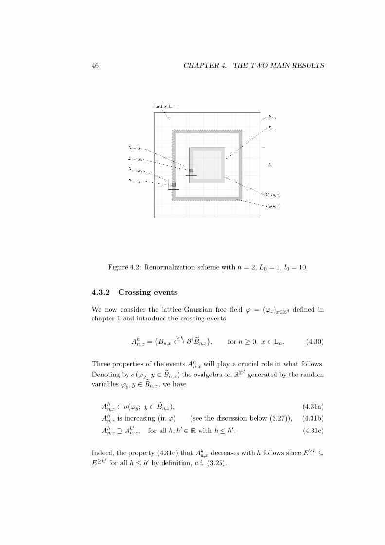
Bn,x := Bx(Ln), for n ≥ 0, x ∈ Ln, (4.24)


where we define Bx(L) = x+ ([0, L)∩Z)d, the box of side length L attachedto x, for any x ∈ Zd and L ≥ 1 (not to be confused with B(x, L)), c.f.Figure 4.2 below (note that Bn,x is closed just on the left-hand side in everydirection). Moreover, we let

Bn,x =⋃

y∈Ln:d(Bn,y ,Bn,x)≤1

Bn,y, n ≥ 0, x ∈ Ln, (4.25)

so that Bn,x;x ∈ Ln defines a partition of Zd into boxes of side length

Ln for all n ≥ 0, and Bn,x;x ∈ Ln, is simply the union of Bn,x and its∗-neighbouring boxes at level n. Furthermore, for n ≥ 1 and x ∈ Ln, Bn,xis the disjoint union of the ld0 boxes Bn−1,y; y ∈ Bn,x ∩Ln−1 at level n− 1it contains. We also introduce the indexing sets

In = n × Ln, n ≥ 0, (4.26)

and given (n, x) ∈ In, n ≥ 1, we consider the sets of labels

H1(n, x) = (n− 1, y) ∈ In−1;Bn−1,y ⊂ Bn,x and Bn−1,y ∩ ∂iBn,x 6= ∅,H2(n, x) = (n− 1, y) ∈ In−1;Bn−1,y ∩ z ∈ Zd; d(z,Bn,x) = bLn/2c 6= ∅.

(4.27)

Note that for any two indices (n − 1, yi) ∈ Hi(n, x), i = 1, 2, we haveBn−1,y1 ∩ Bn−1,y2 = ∅ and Bn−1,y1 ∪ Bn−1,y2 ⊂ Bn,x. Finally, given x ∈Ln, n ≥ 0, we introduce Λn,x, a family of subsets T of

⋃0≤k≤n Ik (soon to

be thought as a binary trees) defined as

Λn,x =

T ⊂

n⋃k=0

Ik; T ∩ In = (n, x) and every (k, y) ∈ T ∩ Ik, 0 < k ≤ n,

has two “descendants” (k − 1, yi(k, y)) ∈ Hi(k, y), i = 1, 2,

such that

T ∩ Ik−1 =⋃

(k,y)∈T ∩Ik

(k − 1, y1(k, y)), (k − 1, y2(k, y)).

(4.28)

Hence, any T ∈ Λn,x can naturally be identified as a binary tree having root(n, x) ∈ In and depth n. Since |H1(n, x)| = c1l0

d−1 and |H2(n, x)| = c2l0d−1,

the following bound on the cardinality of Λn,x is easily obtained,

|Λn,x| ≤ (cl0d−1)2(cl0

d−1)22 · · · (cl0d−1)2n = (cl02(d−1))2(2n−1) ≤ (c0l0

2(d−1))2n ,(4.29)

where c0 ≥ 1 is a suitable constant.


Figure 4.2: Renormalization scheme with n = 2, L0 = 1, l0 = 10.

4.3.2 Crossing events

We now consider the lattice Gaussian free field ϕ = (ϕx)x∈Zd defined inchapter 1 and introduce the crossing events

Ahn,x = Bn,x≥h←→ ∂iBn,x, for n ≥ 0, x ∈ Ln. (4.30)

Three properties of the events Ahn,x will play a crucial role in what follows.

Denoting by σ(ϕy; y ∈ Bn,x) the σ-algebra on RZd generated by the random

variables ϕy, y ∈ Bn,x, we have

Ahn,x ∈ σ(ϕy; y ∈ Bn,x), (4.31a)

Ahn,x is increasing (in ϕ) (see the discussion below (3.27)), (4.31b)

Ahn,x ⊇ Ah′n,x, for all h, h′ ∈ R with h ≤ h′. (4.31c)

Indeed, the property (4.31c) that Ahn,x decreases with h follows since E≥h ⊆E≥h

′for all h ≤ h′ by definition, c.f. (3.25).


4.3.3 The structure of the proof

In this section we give all the P.-F. Rodriguez and A.-S. Sznitman’s ideasto show that

h∗(d) <∞, for all d ≥ 3. (4.32)

To prove (4.32) it enough to construct an explicit level h with 0 < h <∞such that

P(B(0, L)

≥h←→ S(0, L))

decays in L, as L→∞. (4.33)

Actually, the proof of P.-F. Rodriguez and A.-S. Sznitman will even show

that P[B(0, L)≥h←→ S(0, L)] has stretched exponential decay which implies a

(seemingly) stronger result. A second critical parameter is defined

h∗∗(d) = infh ∈ R; for some α > 0, limL→∞

LαP[B(0, L)≥h←→ S(0, L)] = 0,

(4.34)and the following stronger statement is proved:

h∗∗(d) <∞, for all d ≥ 3. (4.35)

For the sake of clarity we investigate later the relevance of this second crit-ical parameter (see Remark 4.3.3) and we now directly prove that h∗(d) <∞, for all d ≥ 3.

As stated before, it is enough to prove (4.33) and to understand why thisimplies that h∗(d) < ∞, for all d ≥ 3. To this second end we note that forevery h ∈ R, given L ≥ 2L0, there exists n ≥ 0 such that 2Ln ≤ L ≤ 2Ln+1

and

η(h) = P(0≥h←→∞

) (1)

≤ P(B(0, L)

≥h←→ S(0, 2L)) (2)

≤(2)

≤ P( ⋃x∈Ln:Bn,x∩S(0,L)6=∅

Bn,x≥h←→ ∂iBn,x

).

(4.36)

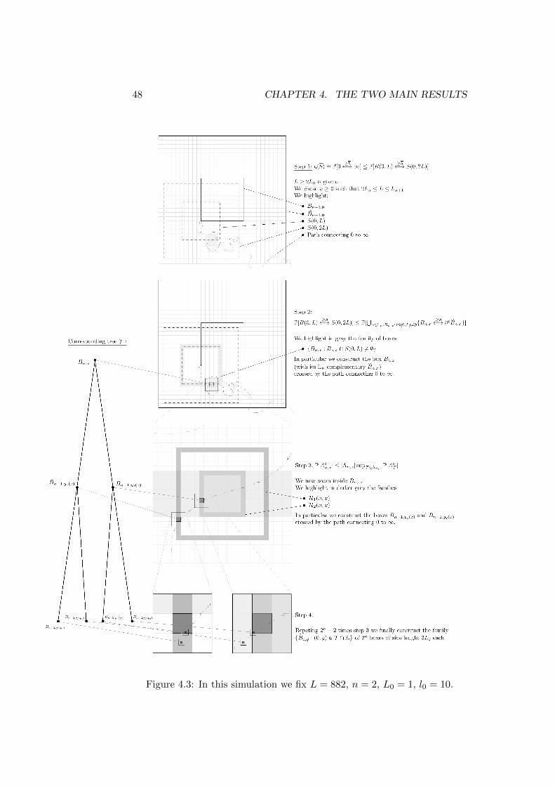
We now comment on the two inequality, helping out with some pictureextracted from a simulation of the renormalization scheme that we realizedduring the master thesis.

1. Consider a realization of the event 0 ≥h←→ ∞, i.e. a path in E≥hϕconnecting 0 to ∞, then this path must also connect the box B(0, L)to the sphere S(0, 2L), c.f. Figure 4.3 (Step 1) below;

2. consider a realization of the event B(0, L)≥h←→ S(0, 2L), i.e. a path

in E≥hϕ connecting B(0, L) to S(0, 2L), then this path must also crossthe box Bn,x for some x ∈ Ln : Bn,x∩S(0, L) 6= ∅ and so must connect

the box Bn,x to the boundary ∂iBn,x of its Ln−neighbourhoods, c.f.Figure 4.3 (Step 2) below.


Figure 4.3: In this simulation we fix L = 882, n = 2, L0 = 1, l0 = 10.


Since the number of sets contributing to the union on the right-handside of (4.36) is bounded by cld−1

0 we obtain

η(h) ≤ cld−10 P

(Bn,x

≥h←→ ∂iBn,x

)= cld−1

0 P(Ahn,x

), (4.37)

where the second term is well-defined (i.e independent of x ∈ Ln) by transla-tion invariance. Now we provide a lemma which separates the combinatorialcomplexity of the number of crossings in Ahn,x from probabilistic estimates,using Λn,x as introduced in (4.28).

Lemma 4.3.2. (n ≥ 0, (n, x) ∈ In, h ∈ R)

P(Ahn,x

)≤ |Λn,x| sup

T ∈Λn,x

P(AhT

), where AhT =

⋂(0,y)∈T ∩I0

Ah0,y. (4.38)

Proof. We use induction on n to show that

Ahn,x ⊆⋃

T ∈Λn,x

AhT , (4.39)

for all (n, x) ∈ In, from which (4.38) immediately follows. When n = 0,(4.39) is trivial. Assume it holds for all (n−1, y) ∈ In−1. For any (n, x) ∈ In,a path in E≥hϕ starting in Bn,x and ending in ∂iBn,x must first cross the boxBn−1,y1 for some (n−1, y1) ∈ H1(n, x), and subsequently B(n−1,y2) for some

(n− 1, y2) ∈ H2(n, x) before reaching ∂iBn,x, c.f. Figure 4.3 (Step 3) below.Thus,

Ahn,x ⊆⋃

(n− 1,yi) ∈ Hi(n, x)

i = 1, 2

Ahn−1,y1∩Ahn−1,y2

.

Upon applying the induction hypothesis to Ahn−1,y1and Ahn−1,y2

separately,the claim (4.39) follows.

Before proceeding, we remark that the event AhT , with h ∈ R and T ∈Λn,x for some (n, x) ∈ In, n ≥ 0, defined in (4.38) depends on 2n boxesof side 3L0 each, c.f. Figure 4.3 (Step 4) below, the first 2n−1 contained inH1(n, x) and the remaining 2n−1 contained in H2(n, x). Moreover, it followsfrom (4.31c) that for any two levels h, h′ ∈ R,

AhT ⊇ Ah′T , whenever h ≤ h′, (4.40)

thus, upon introducing

pn(h) = supT ∈Λn,x

P(AhT), for (n, x) ∈ In, n ≥ 0, (4.41)


which is well-defined (i.e independent of x ∈ Ln) by translation invariance,we obtain

pn(h) ≥ pn(h′), whenever h ≤ h′. (4.42)

Returning to (4.37), using (4.38) and (4.41), we obtain

η(h)(4.38)

≤ cld−10 |Λn,x| sup

T ∈Λn,x

P[AhT ](4.41)= cld−1

0 |Λn,x|pn(h). (4.43)

It remains to explicitly construct an increasing but bounded sequence(hn)n≥0, with finite limit h∞, such that pn(hn) decreases faster than

(c0l02(d−1))−2n , since |Λn,x|

(4.29)

≤ (c0l02(d−1))2n . This result appears in Theo-

rem 4.3.4 where we show that such a sequence (hn)n≥0 exists and pn(hn) ≤(2c0l0

2(d−1))−2n . With this result at hand we can conclude the proof. Weset h = h∞ and using (4.42), we obtain

η(h)(4.42)

≤ cld−10 |Λn,x|pn(hn) ≤ c0l

d−10 2−2n . (4.44)

We finally set ρ = log 2/ log l0, whence 2n = l0nρ = (Ln/L0)ρ. Then, by

adjusting c, c′, (4.44) readily implies

η(h) ≤ c · e−c′Lρ , for all L ≥ 1, (4.45)

for suitable c, c′ > 0 and 0 < ρ < 1. It follows that h ≥ h∗ which completesthe proof.

Remark 4.3.3. Note that (4.45) also implies that h ≥ h∗∗ and so h∗∗(d) <∞,for all d ≥ 3. An important open question is whether h∗ equals h∗∗ or not.

In case the two differ, the decay of P(0≥h←→ S(0, L)

)as L→∞, for h > h∗,

exhibits a sharp transition. Indeed, first note that by definition of h∗, for all

h > h∗, P(0≥h←→ S(0, L)

)→ 0, as L→∞. If h∗∗ > h∗, then by definition of

h∗∗,

for h ∈ (h∗, h∗∗) and any α > 0, lim supn→∞

Ld−1+αP(0≥h←→ S(0, L)

)=∞.

(4.46)

Hence P(0≥h←→ S(0, L)

)decays to zero with L, but with an at most poly-

nomial decay for h ∈ (h∗, h∗∗). However, for h > h∗∗, P(0≥h←→ S(0, L)

)has a stretched exponential decay in L, since P

(0≥h←→ x

)≤ P

(B(0, L)

≥h←→

S(0, 2L)) (4.45)

≤ c(h)e−c′′(h)|x|p whenever 2L ≤ |x|∞ < 2(L+ 1). Recently A.

Drewitz and P.-F. Rodriguez (see [6]) show that

h∗(d) ∼ h∗∗(d), as d→∞ (4.47)

(we write f(x) ∼ g(x) as x → a if limx→a f(x)/g(x) = 1). It is at presentan unresolved question whether both critical parameters are actually equal(in any dimension).


4.3.4 The main Theorem

We now state the aforementioned key result to complete the proof. Most ofthe smarter ideas are presented in Proposition 4.3.5 where Rodriguez andSznitman are able to control the interactions between some crossing events.

Theorem 4.3.4. There exist an increasing but bounded sequence (hn)n≥0,with finite limit h∞, such that

pn(hn) ≤ (2c0l02(d−1))−2n , for all n ≥ 0. (4.48)

First of all we derive a ”recursive bounds” for the probabilities pn(hn),c.f. (4.41) below, along a suitable increasing sequence (hn)n≥0.

Proposition 4.3.5 (L0 ≥ 1, l0 ≥ 100). There exist positive constants c1

and c2 such that, defining

M(n,L0) = c2

(log(2n(3L0)d)

)1/2, (4.49)

then,given any positive sequence (βn)n≥0 satisfying

βn ≥ (log 2)1/2 +M(n,L0), for all n ≥ 0, (4.50)

and any increasing, real-valued sequence (hn)n≥0 satisfying

hn+1 ≥ hn + c1βn(2l−(d−2)0 )n+1, for all n ≥ 0, (4.51)

one haspn+1(hn+1) ≤ pn(hn)2 + 3e−(βn−M(n,L0))2

. (4.52)

Remark 4.3.6. Note that the key-parameter βn controls the size of the in-terval hn+1 − hn in a suitable way that the factor e−(βn−M(n,L0))2

in (4.52)can be small enough.

Before proceeding with the proof of the proposition, we recall again thatthe event AhT , with h ∈ R and T ∈ Λn,x for some (n, x) ∈ In, n ≥ 0, definedin (4.38) depends on 2n boxes of side 3L0 each, c.f. Figure 4.3 (Step 4),the first 2n−1 contained in H1(n, x) and the remaining 2n−1 contained inH2(n, x). In particular if we define the union of these boxes as

KT =⋃

(0,y)∈T ∩I0

B0,y, (4.53)

immediately follows from the definition of AhT that

AhT ∈ σ(ϕy ; y ∈ KT ). (4.54)

We are now ready to prove the proposition.


Proof. We let n ≥ 0, consider some m = (n + 1, x) ∈ In+1 and some treeT ∈ Λm. We decompose

T = m ∩ Tn,y1(m) ∩ Tn,y2(m), (4.55)

where (n, yi(m)), i = 1, 2 are the two descendants of m in T and

Tn,yi(m) = (k, z) ∈ T : Bk,z ⊆ Bn,yi(m), for i = 1, 2, (4.56)

that is T(n,yi(m)) is the (sub-)tree consisting of all descendants of (n, yi(m))in T (in particular it is the left (i=1) or the right (i=2) (sub-)tree in Figure4.3). Thus the union in (4.55) is over disjoint sets. Note in particular thatTn,yi(m) ∈ Λn,yi(m). By construction (see Figure 4.3), the subsets KTn,yi(m)(⊂ Bn,yi(m)

), for i = 1, 2, satisfy KTn,y1(m)

∪ KTn,y2(m)= ∅. For sake of

clarity, and since m and T will be fixed throughout the proof, we abbreviate

Tn,yi(m) = Ti and KTn,yi(m)= Ki, for i = 1, 2. (4.57)

In order to estimate the probability of the event AhT = AhT1 ∩ AhT2 , h ∈ R,

we introduce a parameter α > 0 (that will control the size of the intervalhn+1 − hn to dominate the interactions) and write

P(AhT)

= P(AhT1 ∩A

hT2 ∩

maxK1

ϕ ≤ α)

+ P(AhT1 ∩A

hT2 ∩

maxK1

ϕ > α)

= E[1AhT1

· 1maxK1ϕ≤α · E

[1AhT2

|ϕK1

]]+ P

(AhT1 ∩A

hT2 ∩

maxK1

ϕ > α)

≤ E[1AhT1

· 1maxK1ϕ≤α · P

[AhT2 |ϕK1

]]+ P

(maxK1

ϕ > α),

(4.58)

where maxK1 ϕ = maxϕx; x ∈ K1 and the second line follows becauseAhT1 ∩

maxK1 ϕ ≤ α

is measurable with respect to σ(ϕK1), c.f. (4.54).

We now split the proof in two steps to provide the following two bounds:Bound 1: On the event

maxK1 ϕ ≤ α

, there exist a parameter γ(α) such

thatP[AhT2 |ϕ|K1

]≤ P

(Ah−γT2

)(P(ϕ|K1

≥ −α))−1

. (4.59)

Proof of Bound 1. Using (4.20) and (4.54) applied to AhT2 , and with a slightabuse of notation, we find

P[AhT2 |ϕK1 ] = P[AhT2((ϕx + ux)x∈K2

)], P-almost surely, (4.60)

where ux = Ex[ϕXτK1, τK1 < ∞]. On the event

maxK1 ϕ ≤ α

, we have,

for all x ∈ K2,

ux =∑y∈K1

ϕyPx(XτK1

= y, τK1 <∞)≤ α · Px(τK1 <∞) =: mx(α) (4.61)


which is deterministic and linear in α. Moreover, we can bound mx(α) asfollows. By virtute of (3.16), Px(τK1 < ∞) ≤ cap(K1) · supy∈K1

g(x, y) forall x ∈ K2. Since K1 consists of 2n disjoint boxes of side length 3L0, c.f.(4.57) and (4.53), its capacity can be bounded, using (3.15) and (3.19), ascap(K1) ≤ c2nLd−2

0 . By Lemma 3.2.1 and (4.22) and the observation that|x− y| ≥ c′Ln+1 whenever x ∈ K1 and y ∈ K2, it follows that

mx(α) ≤ c1(2G(0))−1/2 · α · 2nl−(n+1)(d−2)0 =:

γ

2, for x ∈ K2, (4.62)

which defines the constant c1 from (4.51), and the factor (2G(0))−1/2 is keptfor later convenience.

Returning to the conditional probability P[AhT2 |ϕK1

], we first observe

that, on the event

maxK1 ϕ ≤ α, and for any x ∈ K2, the inequality

ϕx + ux ≥ h implies

ϕx −mx(α) ≥ h− ux −mx(α)(4.61)

≥ h− 2mx(α)(4.62)

≥ h− γ. (4.63)

Hence, on the event

maxK1 ϕ ≤ α,

P[AhT2 |ϕK1

] (4.60)= P

[AhT2

((ϕx + ux)x∈K2

)]

≤ P[AhT2

((ϕx +mx(α))x∈K2

)]= P

[Ah−γT2 |ϕK1 = −α

],

(4.64)

where the last equality follows by (4.20), nothing that, on the event ϕ|K1=

−α, we have ux = mx(−α) = −mx(α) for all x ∈ K2, c.f. (4.61). ApplyingLemma 4.3.1 to the right-hand side of (4.64), we immediately obtain that,on the event

maxK1 ϕ ≤ α

,

P[AhT2 |ϕK1

]≤ P

(Ah−γT2 |ϕ|K1

≥ −α)≤ P

(Ah−γT2

)(P(ϕ|K1

≥ −α))−1

. (4.65)

Bound 2:

P(

maxK1

ϕ > α)≤ min

1

2, e

−(

α√2G(0)

−M(n,L0))2. (4.66)

Proof of Bound 2. By virtue of the BTIS-inequality (see section 2.2), forarbitrary ∅ 6= K ⊂⊂ Zd, we have

P(

maxK

ϕ > α)≤ exp

− (α− E[maxK ϕ])2

2G(0)

, if α > E

[maxK

ϕ],

(4.67)and by Proposition 3.1.1 we know that

E[

maxK

ϕ]≤ c√

log |K|. (4.68)


In the relevant case K = K1 with |K1| = 2n(3L0)d, we thus obtain

E[

maxK1

ϕ]≤ c2(2G(0) log(2n(3L0)d))1/2 (4.49)

=√

2G(0) ·M(n,L0) (4.69)

where the first inequality defines the constant c2 from (4.49). We now require

α/√

2G(0) ≥√

log 2 +M(n,L0) (4.70)

where the factor log 2 is kept for later convenience, thus (4.67) applies andyields

P(

maxK1

ϕ > α)≤ min

1

2, e

−(

α√2G(0)

−M(n,L0))2, (4.71)

sinceα−E[maxK1

ϕ]√2G(0)

≥ α√2G(0)

−M(n,L0) ≥√

log 2.

We now insert (4.59) into (4.58), noting that, since ϕ has the same law as−ϕ, we have P(ϕ|K1

≥ −α) = 1−P(minK1 ϕ < −α) = 1−P(maxK1 ϕ > α),to get

P(AhT)≤ P

(AhT1

)· P(Ah−γT2

)·(

1− P(

maxK1

ϕ > α))−1

+ P(

maxK1

ϕ > α).

(4.72)Using that (1−x)−1 ≤ 1+2x for all 0 ≤ x ≤ 1/2 (with x = P(maxK1 ϕ > α)),we finally obtain, for all α satisfying (4.70) and h′ ≥ h,

P(Ah′T)≤ P

(AhT)≤ P

(AhT1

)· P(Ah−γT2

)+ 3 · P

(maxK1

ϕ > α)

(4.66)

≤ P(AhT1

)· P(Ah−γT2

)+ 3e−

(β−M(n,L0)

)2

,

(4.73)

where we have set β = α/√

2G(0). The claim (4.52) now readily followsupon tacking suprema over all T ∈ Λn+1,x on both side of (4.73), lettingβn := β, hn := h − γ ∈ R (h was arbitrary), hn+1 = h′, so that requiringhn+1 = h′ ≥ hn + γ, by virtute of (4.62), is nothing but (4.51). Noting that(4.70) for βn = β, we precisely recover (4.50). This concludes the proof ofProposition 4.3.5.

We now propagate the estimate (4.52) inductively. To this end, we firstdefine, for all n ≥ 0,

βn = (log 2)1/2 +M(n,L0) + 2(n+1)/2(n1/2 +K

1/20

), (4.74)

where K0 > 0 is a certain parameter to be specified below (it will allow usto start the induction). Note in particular that condition (4.50) holds forthis choice of (βn)n≥0. In the next proposition, we inductively derive boundsfor pn(hn), n ≥ 0, given any sequence (hn)n≥0 satisfying the assumptions ofProposition 4.49, provided the induction can be initiated.


Proposition 4.3.7. Assume h0 ∈ R and K0 ≥ 3(1− e−1)−1 =: B are suchthat

p0(h0) ≤ e−K0 , (4.75)

and let the sequence (hn)n≥0 satisfy (4.51) with (βn)n≥0 as defined in (4.74).Then,

pn(hn) ≤ e−(K0−B)2n , for all n ≥ 0. (4.76)

The strategy of the proof is to define a sequence (Kn)n≥0 such thatKn ≥ K0 − B for all n ≥ 0 and pn(hn) ≤ e−Kn2n for all n ≥ 0. This allowsus to immediately conclude the proof.

Proof. We define a sequence (Kn)n≥0 inductively by

Kn+1 = Kn− log(1+eKn(32−(n+1)

e−2−(n+1)(βn−M(n,L0))2)), for all n ≥ 0

(4.77)

with βn give by (4.74). Note that the factor 32−(n+1)e−2−(n+1)(βn−M(n,L0))2

is the 2n+1−th root of the remainder term on the right-hand side of (4.52)(i.e. 3e−(βn−M(n,L0))2

). Note also that Kn ≤ K0 for all n ≥ 0 since Kn isdecreasing. Moreover, we have

• Kn ≥ K0 −B for all n ≥ 0.

This is clear for n=0.

When n ≥ 1, first note that by the definition of Kn, for all n ≥ 1,

Kn = K0 −n−1∑m=0

log(

1 + eKm(32−(m+1)e−2−(m+1)(βm−M(m,L0))2

)).

(4.78)

Moreover

(βm −M(m,L0))2 = ((log 2)1/2 + 2(m+1)/2(m1/2 +K1/20 ))2

≥ log 2 + 2m+1(m1/2 +K1/20 )2 ≥ 2m+1(m+K0),

(4.79)

for all m ≥ 0, which, inserted into (4.78), yields

Kn ≥ K0 −∞∑m=0

log(

1 + eKm(32−(m+1)e−2−(m+1)(2m+1(m+K0)))

)= K0 −

∞∑m=0

log(

1 + eKm(32−(m+1)e−m−K0)

)≥ K0 − 3

∞∑m=0

e−m = K0 − 3(1− e−1)−1 = K0 −B,

(4.80)


where we have used Kn ≤ K0 and log(1 + x) ≤ x for all x ≥ 0 in thelast inequality.

• pn(hn) ≤ e−Kn2n for all n ≥ 0.

We show the result by induction on n.

The inequality holds for n = 0 by assumption (4.75).

Assume now it holds for some n. By condition (4.52), we find

pn+1(hn+1) ≤ pn(hn)2 + 3e−(βn−M(n,L0))2

≤ (e−Kn2n)2 + 3e−(βn−M(n,L0))2

≤[e−Kn

(1 + eKn32−(n+1)

e−2−(n+1)(βn−M(n,L0)2)]2n+1

= e−Kn+12n+1.

(4.81)

This concludes the proof of the proposition.

We will now prove the main theorem (Theorem 4.3.4) of this sectionusing Proposition 4.3.7.

Proof (of Theorem 4.3.4). We select K0 appearing in Proposition 4.3.7 asfollow:

K0 = log(2c0l2(d−1)0 ) +B (see (4.29) for the definition of c0). (4.82)

Moreover we will solely consider sequences (hn)n≥0 with

h0 > 0, hn+1 − hn = c1βn(2l−(d−2)0 )n+1, for all n ≥ 0, (4.83)

so that condition (4.51) is satisfied. We recall that βn is given by (4.74),which now reads

βn = (log 2)1/2+c2(log(2n(3L0)d))1/2+2(n+1)/2(n1/2+(log(2c0l2(d−1)0 )+B)1/2)

(4.84)where we have substituted M(n,L0) from (4.49) and K0 from (4.82). Notethat L0, l0 and h0 are the only parameters which remain to be selected.We observe that the sequence defined in (4.83) has a finite limit h∞ =limn→∞ hn for every choice of L0, l0 and h0. Indeed, βn as given by (4.84)satisfies βn ≤ c(L0, l0)2n+1 for all n ≥ 0, hence

h∞ = h0 + c1

∞∑n=0

βn(2l−(d−2)0 )n+1 ≤ h0 + c′(L0, l0)

∞∑n=0

(4l−(d−2)0 )n+1 <∞,

(4.85)


since we assumed l0 ≥ 100. We set

L0 = 10, l0 = 100, (4.86)

and now show with Proposition 4.3.7 that there exists h0 > 0 sufficientlylarge such that

pn(hn) ≤ (2c0l02(d−1))−2n , for all n ≥ 0. (4.87)

To this end, we note that p0(h0) defined in (4.41)

p0(h0) = P(B0,x=0

≥h0←−→ ∂iB0,x=0

)≤ P

(maxB0,x=0

ϕ ≥ h0

)≤ exp

−

(h0 − E

[max

B0,x=0ϕ])2

2G(0)

,

(4.88)

where the last inequality holds when h0 > c (e.g using Proposition 3.1.1 tobound E

[max

B0,x=0ϕ]) thanks to BTIS-inequality (see (2.10)). In particu-

lar, since K0 in (4.82) is completely determined by the choices (4.86), we seethat p0(h0) ≤ e−K0 for all h0 ≥ c, i.e. condition (4.75) holds for sufficientlylarge h0. by Proposition 4.3.7, setting h0 = c, we obtain

pn(hn)(4.76)

≤ e−(K0−B)2n (4.82)= (2c0l

2(d−1)0 )−2n for all n ≥ 0. (4.89)

This result concludes the proof.

Chapter 5

A generalization of the BLMproof

In both two article [3] and [11] it is remarked that the BLM proof can’t beeasily gereralized to all d ≥ 3 since, in d ≥ 4, a infinite connected set maynot be recurrent for the simple random walk on Zd. In this chapter we tryto prove that this is not an issue, since, an infinite cluster over a level h,if it exists than it has positive density by Newman and Schulman theorem,and in particular, using the well-known Wiener’s test, it is recurrent for thesimple random walk on Zd.

5.1 Finite energy property for the DGFF

The first step is to prove that Theorem 3.6.2 holds for the level-sets percola-tion for the DGFF. We consider the measurable map φh from Ω = RZd intoΩ = 0, 1Zd as defined in (3.26) and the associated pushforward measure

Ph := φh∗(P) on Ω = 0, 1Zd . We need to show that

1. Ph is translation invariant;

2. Ph has the finite energy property;

The first property is a trivial consequence of the translation-invariance prop-erty of P. For the second property (that is claimed without proof in [11],Remark 1.6) we give a proof in the following lemma.

Lemma 5.1.1. The probability measure Ph for the DGFF has the finiteenergy property.

Proof. We need to check that for all x ∈ Zd and η = 0 or 1, if U ⊂ Ωx andPh(U × 1ϕx≥h = η) 6= 0 then Ph(U × 1ϕx≥h = 1 − η) 6= 0. Fromthe translation invariance of the DGFF, it is sufficient to show that for all

59

60 CHAPTER 5. A GENERALIZATION OF THE BLM PROOF

U ⊂ Ωx, setting U := (φh)−1(U), holds:

P(U × ϕ0 ≥ h) 6= 0 if and only if P(U × ϕ0 < h) 6= 0. (5.1)

Suppose that P(U×ϕ0 ≥ h) > 0. Since the measure P is tight (for examplefor the Ulam’s theorem), then there exist L > 0 such that

P(

U ∩ϕx ∈ [h− L, h+ L]; |x| = 1

×ϕ0 ∈ [h, h+ L]

)> 0. (5.2)

Denoting UL1 :=ϕx ∈ [h − L, h + L]; |x| = 1

∈ Fx∈Zd;|x|=1 =: F1 and

using the local Markov property of the DGFF, we obtain

P(U ∩ UL1

×ϕ0 ∈ [h, h+ L]

)= E

[E[1U∩UL1 ×ϕ0∈[h,h+L]|F1

]]= E

[1UL1· E[1U |F1

]· E[1ϕ0∈[h,h+L]|F1

]].

(5.3)

Under UL1 , there exists a constant εL > 0 such that

E[1ϕ0∈[h,h+L]|F1

]≤ εL · E

[1ϕ0∈[h−L,h)|F1

], a.s. . (5.4)

Indeed, using standard results for conditional Gaussian vectors, E[ϕ0|F1] isa linear combination of the random variables ϕx for x ∈ Zd such that |x| = 1,denoted by Y :=

∑x∈Zd;|x|=1 λxϕx, and more generally, denoting by qµ,σ2(x)

the density of a Gaussian random variable with mean µ and variance σ2, wehave

E[1ϕ0∈[h,h+L]|F1

]=

∫R1[h,h+L](x)qY,σ2(x)dx, (5.5)

where σ2 = E[(ϕ0 − Y )2]. Finally, noting that under UL1 , Y ∈ [2d(h −L), 2d(h− L)], the bound in (5.4) follows from (5.5).

Summing up and repeating the same computation as in (5.3), we obtain

0 < P(U ∩ UL1

×ϕ0 ∈ [h, h+ L]

)≤ εL · P

(U ∩ UL1

×ϕ0 ∈ [h− L, h)

)≤ εL · P

(U × ϕ0 < h

).

(5.6)

Since the other implication is similar, this concludes the proof.

Now, setting ρh := P(|Ch(0)| = ∞

)and noting that ρh > 0 for all

h < h∗(d), we have the following result

Proposition 5.1.2. For all h < h∗(d), conditioning on the event 0 ≥h←→∞,

D(Ch(0)

)= ρh, a.s. . (5.7)

In particular, conditioning on the event 0 ≥h←→ ∞, D(Ch(0)

)> 0 almost

surely.

We are now ready to give our new proof of the existence of a phasetransition for the level-set percolation for the DGFF on Zd, for all d ≥ 3.

5.2. THE SETUP 61

5.2 The setup

We start this section by introducing some definition and notation. LetVn, n ∈ N be a collection of boxes as defined in equation (3.31). We denoteby Λ := Vm, for some m ∈ N, a smaller box such that |Vn| |Λ|. Rememberthat Ch(0) denote the (random) cluster containing the origin and define theevents

ChVn =ϕ ∈ Ω: Ch(0) ∩ ∂iVn 6= ∅

, for all h ∈ R and n ∈ N. (5.8)

Let ShVn be the following collection of subsets of Vn, for all n ∈ N,

ShVn =K ⊆ Vn : 0 ∈ K, K is connected and K ∩ ∂iVn 6= ∅; and

ρh

2<|K ∩ Vm|md

< 2ρh, ∀m ∈ N s.t. n/2 ≤ m ≤ n.

(5.9)

Note that the family ShVn is a collection of the possible shapes for the con-

nected component of the infinite cluster Ch(0) inside Vn (see Figure 5.1).Define for a paricular K ∈ ShVn the event

EhK =ϕ ∈ Ω : ϕx ≥ h,∀x ∈ K and ϕx < h,∀x ∈ ∂VnK

, (5.10)

where ∂VnK = ∂K ∩ Vn.Since in many of the following lemmas the parameter h ∈ R will be

fixed, we will omit the appendix h on the sets, families and events previouslydefined, unless absolutely necessary. Moreover, from now till the end, we

suppose by contradiction that, for any level h, the event 0 ≥h←→∞ occourswith positive probability, i.e., h∗(d) =∞.

5.3 The technical lemmas

Before state and prove the four technical lemmas, we note that (from Propo-sition 5.1.2) we have

limn→∞

|C(0)(ϕ) ∩ Vn|nd

= ρ, for a.a. ϕ ∈ 0 ≥h←→∞. (5.11)

Since (Ω,F ,P) is a finite measure space, from the Egorov’s theorem we know

that for all δ > 0, there exists a measurable subset Ωδ ∈ F , Ωδ ⊂ 0≥h←→∞,

such that

P(0 ≥h←→∞ \ Ωδ) <δ and the limit (5.11) is uniform on Ωδ, i.e.,

limn→∞

supϕ∈Ωδ

∣∣∣ |C(0)(ϕ) ∩ Vn|nd

− ρ∣∣∣ = 0.

(5.12)


Figure 5.1: In this example we fix a level h ∈ R and we paint in black thesites over the level h. Moreover we highlight the sets Vn, Λ, C(0)∩Vn, and∂VnK. Note that K = C

(C(0)(ϕ), Vn

).

In particular, there exists n0 = n0(δ) ∈ N such that for all n ≥ n0 wehave

ρ

2<|C(0)(ϕ) ∩ Vn|

nd< 2ρ, for all ϕ ∈ Ωδ. (5.13)

We claim that the bound (5.13) holds also for the connected component inC(0)(ϕ) ∩ Vn containing 0, denoted by C

(C(0)(ϕ), Vn

). The proof of this

claim still open for the moment.

Remark 5.3.1. We are considering the connected component C(C(0)(ϕ), Vn

)instead of the whole set C(0)(ϕ) ∩ Vn in order to obtain a disjoint union inthe left hand side of equation (5.14).

We can now state the first technical lemma.

Lemma 5.3.2. Let CVn be the event defined in (5.8). Then for all n ≥ 2n0,

1. CVn ∩ Ωδ is contained in the disjoint union of the events EK , i.e.,

CVn ∩ Ωδ ⊆⊔

K∈SVn

EK , (5.14)

and if K,K ′ ∈ SVn and K 6= K ′, then EK ∩ EK′ = ∅.

2. P(CVn ∩ Ωδ) ≥ P(0 ≥h←→∞ ∩ Ωδ

)and P(EK) > 0 for all K ∈ SVn .

5.3. THE TECHNICAL LEMMAS 63

Proof. Fix n ≥ 2n0. We start by proving that CVn ∩ Ωδ ⊆⊔K∈SVn

EhK . If

ϕ ∈ CVn ∩ Ωδ then C(0)(ϕ) intersects the inner boundary of Vn, that isCh(0) ∩ ∂iVn 6= ∅. Setting K := C

(C(0)(ϕ), Vn

)then K ∈ SVn since

• K ⊆ Vn, 0 ∈ K, K is connected and K ∩ ∂iVn 6= ∅;

• From the claim below relation (5.13) and the fact that n ≥ 2n0 wehave

ρ

2<|K ∩ Vm|md

< 2ρ, for all m ∈ N s.t. n/2 ≤ m ≤ n. (5.15)

In particular EK occurs. The events EK are disjoint by definition. Part (2)is obvious.

We now show the key point of our proof, namely, the fact that a set withpositive density is recurrent for a symmetric random walk in Zd.

Lemma 5.3.3. For some 0 < u ≤ 1 and for all Λ, we can take Vn = Vn(Λ)large enough so that

1

|Λ|∑x∈Λ

fK(x) ≥ u, for all K ∈ SVn and for all x ∈ Λ, (5.16)

where fK(x) is defined in (3.22).

Proof. First of all we show that a set A ⊆ Zd satisfying

ρ

2<|A ∩ Vm|md

< 2ρ, for all m ∈ N, (5.17)

is recurrent. In order to prove this result we applay Theorem 3.4.1 and weshow that T [A] = +∞, where T[A] is defined in (3.21).

From (5.17) we have, for all l ≥ 1,∣∣Al∣∣ (3.20)=

∣∣A ∩ y ∈ Zd; 2l < |y|∞ ≤ 2l+1∣∣ =

∣∣A ∩ V2l+2

∣∣− ∣∣A ∩ V2l+1

∣∣>ρ

2(2l+2)

d − 2ρ(2l+1)d

= ρ · 2(l+1)d(2d−1 − 2) > ρ · 2ld,(5.18)

Similarly, using the other bound in (5.17), we can find the following estimate∣∣Al∣∣ < ρ2(l+1)d(2d+1 − 2−1) ≤ c · 2ld, for all l ≥ 1. (5.19)

Now using estimate (3.18) and (5.18) we obtain

cap(Al) ≥ρ · 2ld

Ml, for all l ≥ 1, (5.20)


where Ml = supz∈Al

(∑y∈Al G(z, y)

). Note that, using the classical bounds

on the Green function (see Theorem 3.2.1), we obtain

Ml ≤ supz∈Al

( ∑y∈Al

c′

(|y − z|∞ + 1)d−2

), for all l ≥ 1. (5.21)

and taking, for each l ≥ 1, a box VL(l) such that |VL(l)| ≥ |Al|, we have

supz∈Al

( ∑y∈Al

c′

(|y − z|∞ + 1)d−2

)≤

∑y∈VL(l)

c′

(|y|∞ + 1)d−2, for all l ≥ 1,

(5.22)since, fixed an element z ∈ Al, we can easily construct an injective corre-spondence Γl between Al and VL(l) such that at each element y ∈ Al, assignan element Γl(y) ∈ VL(l), with the property that |y − z|∞ ≥ |Γl(y)|∞.

By (5.19) there exists an odd number L(l) and a constant c > 0 suchthat L(l) ≤ c · 2l and |VL(l)| ≥ |Al|. In particular, noting that∣∣y ∈ VL; |y|∞ = n

∣∣ = |V2n+1| − |V2n−1|= (2n+ 1)d − (2n− 1)d ≤ c · nd−1, for all n ≥ 1,

(5.23)

and using the bound (5.21) and (5.22), we obtain

Ml ≤ c′ + c′′c·2l∑n=1

nd−1

(n+ 1)d−2≤ c′ + c′′

c·2l∑n=1

n ≤ c · 22l, for all l ≥ 1. (5.24)

Finally from (5.20) and (5.24) we conclude

cap(Al) ≥ c · 2l(d−2), for all l ≥ 1, (5.25)

and so

T [A] ≥∞∑l=1

c =∞. (5.26)

Now from the proof of the Wiener’s test (see Theorem 3.4.1) we know that,for all Λ and 0 < u < 1, exists N = N(u,Λ) > 0 such that if a set A ⊂ Zdsatisfies T [A] > N, then fA(x) > u, for all x ∈ Λ.

Finally fixing u, for all Λ, from the divergence of (5.26), we can imme-diately conclude that there exists Vn(Λ) large enough such that

T [K] > N, for all K ∈ SVn , (5.27)

and sofK(x) > u, for all K ∈ SVn and for all x ∈ Λ. (5.28)

In particular

fK(x) > u, for all K ∈ SVn and for all x ∈ Λ. (5.29)

5.3. THE TECHNICAL LEMMAS 65

The following lemma gives us an important lower bound for the functionE[ϕx|EK ] for all x ∈ ∂K.

Lemma 5.3.4. For h <∞ large enough there is a constant c > 0 such thatfor all Vn large enough

E[ϕx|EK ] ≥ c, for all x ∈ ∂K, all K ∈ SVn . (5.30)

Proof. This lemma is proved in [3], Lemma 3, p. 1264. We are not able tofollow the last part of the proof where the Ruelle’s superstability estimateis applied.

The following lemma generalizes the previous lower bound for the func-tion E[ϕx|EK ], for all x ∈ Zd. The proof of this lemma is based on the resultstated in Lemma 1.5.2.

Lemma 5.3.5. For h < ∞ large enough there exists a positive constantc > 0 such that for all Vn large enough

E[ϕx|EK ] ≥ c · fK(x) for all x ∈ Zd, all K ∈ SVn , (5.31)

where K = K ∪ ∂K.

Proof. For all K ⊂⊂ Zd, applying Lemma 1.5.5 we have, for all x ∈ Zd \K,

E[ϕx|FK ](w) = Ex[ωXτK, τK <∞], P-a.s. , (5.32)

where FK = σ(ϕx; x ∈ K). Obviously, for all K ∈ SVn , EK ∈ FK and inparticular we have

E[ϕx|EK ] = E[Ex[ϕXτK, τK <∞]|EK ], for all x ∈ Zd \K, (5.33)

Fixed h <∞ large enough, for all Vn large enough, applying Lemma 5.3.4,we obtain,

E[ϕx|EK ] = E[Ex[ϕXτK, τK <∞]|EK ]

= E[∑k∈∂K

Px(XτK= k, τK <∞)ϕk|EK ]

=∑k∈∂K

E[ϕk|EK ]Px(XτK= k, τK <∞)

≥ c · fK(x), for all x ∈ Zd \K,

(5.34)

and in particular, we can conclude that for all Vn large enough,

E[ϕx|EK ] ≥ c · fK(x) for all x ∈ Zd, all K ∈ SVn . (5.35)


5.4 The conclusion of the proof

We are now ready to conclude the proof.

Proof. Lemma 5.3.5 says that for h <∞ large enough there exists a positiveconstant c > 0 such that for all Vn large enough

E[ϕx|EK ] ≥ c · fK(x) for all x ∈ Zd, all K ∈ SVn . (5.36)

Combining Lemma 5.3.3 with (5.36): there is a costant u > 0 such that forall Λ, we can choose Vn = Vn(Λ) large enough such that

1

|Λ|∑x∈Λ

E[ϕx|EK ] ≥ u, for all K ∈ SVn . (5.37)

By Lemma 5.3.2, denoting SΛ :=∑

x∈Λ ϕx and Un :=⊔K∈SVn

EK , we have

E[(SΛ)2

]≥ E

[(SΛ)21Un

]=

∑K∈SVn

E[(SΛ)21EK

]=

∑K∈SVn

E[(SΛ)2|EK

]P[EK ]

(5.38)and by the Cauchy-Schwartz inequality

≥∑

K∈SVn

E[SΛ|EK

]2P[EK ] ≥∑

K∈SVn

u2|Λ|2P[EK ], (5.39)

where we used (5.37) for the last inequality. Now, by Lemma 5.3.2 again, in

particular using that CVn ∩ Ωδ ⊆⊔K∈SVn

EhK and P(CVn ∩ Ωδ) ≥ P(0 ≥h←→

∞ ∩ Ωδ

), we obtain

≥ u2|Λ|2P(CVn ∩ Ωδ) ≥ u2|Λ|2P(0 ≥h←→∞ ∩ Ωδ

). (5.40)

Since this chain of inequalities holds for all Λ and E[(

(1/|Λ|)SΛ

)2]→ 0, for

Λ ↑ Zd, we obtain that P(0 ≥h←→∞∩Ωδ

)= 0. Finally taking the limit for

δ → 0, we get P(0 ≥h←→∞

)= 0, for all h > h.

This completes the proof.

Chapter 6

Open problems

We summarize in this final chapter the two open problems that appear inour new proof. We tried to be as independent as possible from the previouschapter with the notation in order to be accessible to lay readers.

Let (ϕx)x∈Zd be a Discrete Gaussian Free Field on Zd and Vn be a boxof size n ∈ N centered in the origin 0.

Problem 1.We claim that the connected component containing 0 inthe cluster C(0)(ϕ) inside Vn, denoted by C

(C(0)(ϕ), Vn

), satisfies for some

ρ > 0,ρ

2<|C(C(0)(ϕ), Vn

)|

nd< 2ρ,

for all configurations ϕ contained in an arbitrary large subset of the config-urations such that the origin 0 lies in the infinite cluster over level h. Seethe claim below equation (5.13) for a more precise statement.

We belive that using an ”ergodic argument” the result could be prove.Problem 2. This is the main problem in our proof. We would like to

use a result stated in [3, Lemma 3, p. 1264] but we are not able to follow thelast part of the proof where the Ruelle’s superstability estimate is applied.The result is intuitive but it seems to be extremely technical to prove. Wegive a statement: for a box Vn we define

SVn =K ⊆ Vn : 0 ∈ K, K is connected, K ∩ ∂iVn 6= ∅

.

Lemma. For h < ∞ large enough there is a constant c > 0 such that forall boxes Vn large enough

E[ϕx

∣∣∣ϕx ≥ h,∀x ∈ K and ϕx < h,∀x ∈ ∂VnK]≥ c, for all x ∈ ∂K,

all K ∈ SVn ,

where ∂VnK = ∂K ∩ Vn.

Intuitively the result states that the field on the external boundary of acluster over level h is in mean strictly positive if h is big enough.

67

68 CHAPTER 6. OPEN PROBLEMS

Bibliography

[1] R.J. Adlre and J.E. Taylor. Random fields and geometry. Springer, NewYork (2007).

[2] C.Borell, The Brunn-Minkowski inequality in Gauss space, Invent.Math., 30 (1975), 205-216.

[3] J. Bricmont, J. L. Lebowitz and C. Maes. Percolation in strongly corre-lated systems: the massless Gaussian field. J. Stat. Phys., 48(5/6): pp.1249-1268 (1987).

[4] R.M. Burton and M. Keane. Density and Uniqueness in Percolation.Commun. Math. Phys. 121: pp. 501-505 (1989).

[5] L.Chaumont and M.Yor, Exercises in Probability: A Guided Tour fromMeasure Theory to Random Processes, via Conditioning, Cambridge Se-ries in Statistical and Probabilistic Mathematics, Cambridge UniversityPress, Cambridge, UK, 2003.

[6] A. Drewitz and P.-F. Rodriguez. High-dimensional asymptotics for per-colation of Gaussian free field level sets. Electron. J. Probab. 20(47), pp.1-39 (2015).

[7] S. Friedli and Y. Velenik. Statistical Mechanics of Lattice Sys-tems: a Concrete Mathematical Introduction. Book project avaiable athttp://www.unige.ch/math/folks/velenik/smbook/index.html.

[8] G. Giacomin. Aspects of statistical mechanics of random sur-faces. Notes of the lectures given at IHP, fall 2001 (re-vised version, November 2002), avaiable at https://www.lpma-paris.fr/modsto/users/giacomin/publications.

[9] G.F. Lawler. Intersection of random walks. Birkhauser, Basel (1991).

[10] C.M. Newman and L.S. Schulman. Infinite clusters in percolation mod-els. J. Stat. Phys., 26: pp. 613-628 (1981).

69

70 BIBLIOGRAPHY

[11] P.-F. Rodriguez and A.-S. Sznitman. Phase transition and level-set per-colation for the Gaussian free field. Commun. Math. Phys. 320(2): pp.571–601 (2013).

[12] V. Sidoravicius and A.S. Sznitman. Connectivity bounds for the vacantset of random interlacements. Ann. Inst. Henri Poincare, Probabilites etStatistiques, 46(4): pp. 976-990 (2010).

[13] F. Spitzer. Principle of Random Walk. Springer, New York, 2nd ed.(1976).

[14] A.S. Sznitman. Vacant set of random interlacements and percolation.Ann. Math. 171: pp. 2039-2087 (2010).

[15] B.S.Tsirelson, I.A.Ibragimov, and V.N. Sudakov, Norms of Gaussiansample functions, in Proceedings of the 3rd Japan-USSR Symposium onProbability Theory (Tashkent, 1975), Lecture Notes in Mathematics, Vol.550, Springer-Verlag, Berlin, 1976, 20-41.

percolazione per insiemi di livello del gaussian free eld

Documents