perceiving 3d from 2d images
TRANSCRIPT
Chapter 12
Perceiving 3D from 2D Images
This chapter investigates phenomena that allow 2D image structure to be interpreted interms of 3D scene structure. Humans have an uncanny abilty to perceive and analyze thestructure of the 3D world from visual input. Humans operate e�ortlessly and often havelittle idea what the mechanisms of visual perception are. Before proceeding, three pointsmust be emphasized. First, while the discussion appeals to analytical reasoning, humansreadily perceive structure without conscious reasoning. Also, many aspects of human visionare still not clearly understood. Second, although we can nicely model several vision cuesseparately, interpretation of complex scenes surely involves competitive and cooperative pro-cesses using multiple cues simultaneously. Finally, our interest need not be in explaininghuman visual behavior at all, but instead be in solving a particular application problem ina limited domain, which allows us to work with simpler sets of cues.
The initial approach used in this chapter is primarily descriptive. The next section dis-cusses the intrinsic image, which is an intermediate 2D representation that stores importantlocal properties of the 3D scene. Then we explore properties of texture, motion, and shapethat allow us to infer properties of the 3D scene from the 2D image. Although the emphasisof this chapter is more on identifying sources of information rather than mathematicallymodeling them, the �nal sections do treat mathematical models. Models are given for
perspective imaging, computing depth from stereo, and for relating �eld of view to resolu-tion and blur via the thin lens equation. Other mathematicalmodeling is left for Chapter 13.
12.1 Intrinsic Images
It is convenient to think of a 3D scene as composed of object surface elements that are illu-minated by light sources and that project as regions in a 2D image. Boundaries between 3Dsurface elements or changes in the illumination of these surface elements result in contrastedges or contours in the 2D image. For simple scenes, such as those shown in Figures 12.1and 12.2, all surface elements and their lighting can be respresented in a description ofthe scene. Some scientists believe that the major purpose of the lower levels of the humanvisual system is to construct some such representation of the scene as the base for furtherprocessing. This is an interesting research question, but we do not need an answer in orderto proceed with our work. Instead, we will use such a representation for scene and image
1
2 Computer Vision: Mar 2000
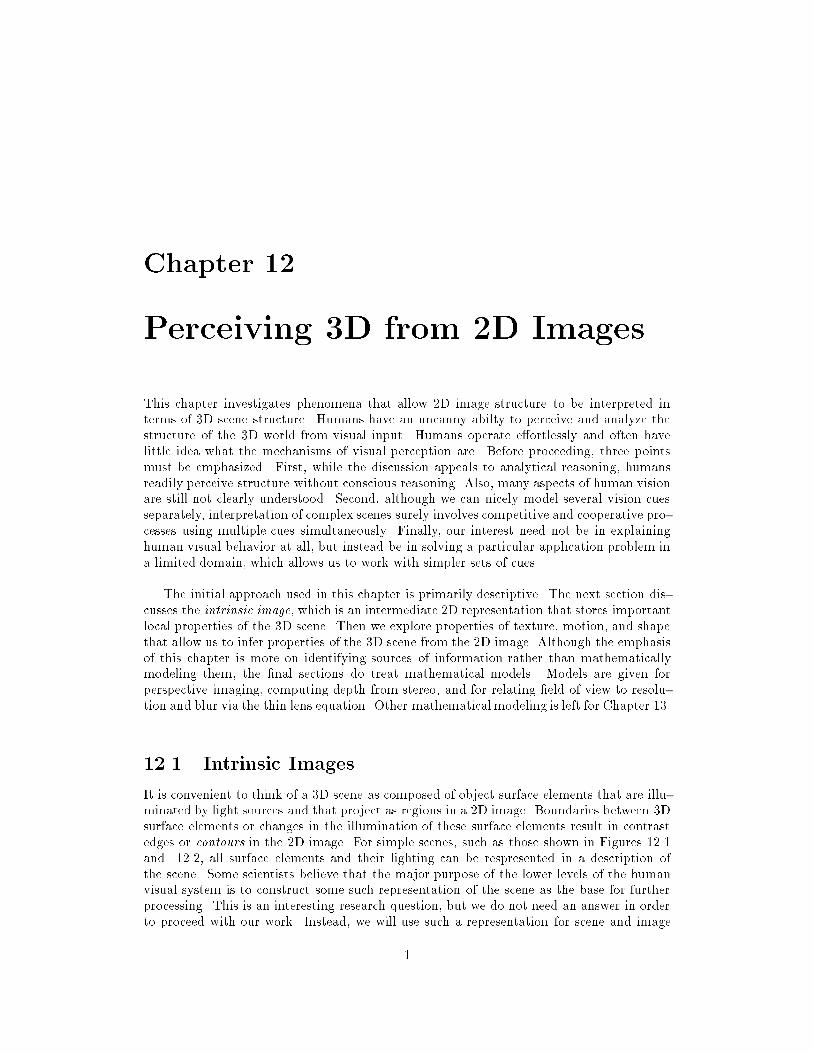
Figure 12.1: (Left) Intensity image of three blocks and (right) result of 5x5 Prewitt edgeoperator.
������
������
���������
���������
���������
���������
+
+
+
MS
S
S
S
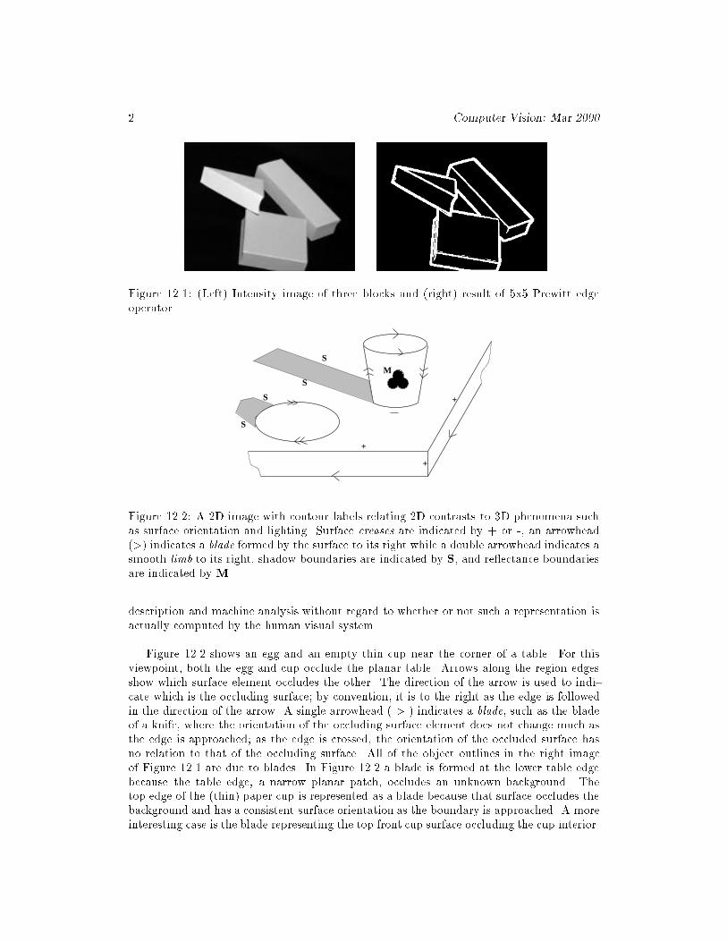
Figure 12.2: A 2D image with contour labels relating 2D contrasts to 3D phenomena suchas surface orientation and lighting. Surface creases are indicated by + or -, an arrowhead(>) indicates a blade formed by the surface to its right while a double arrowhead indicates asmooth limb to its right, shadow boundaries are indicated by S, and re ectance boundariesare indicated by M.
description and machine analysis without regard to whether or not such a representation isactually computed by the human visual system.
Figure 12.2 shows an egg and an empty thin cup near the corner of a table. For thisviewpoint, both the egg and cup occlude the planar table. Arrows along the region edgesshow which surface element occludes the other. The direction of the arrow is used to indi-cate which is the occluding surface; by convention, it is to the right as the edge is followedin the direction of the arrow. A single arrowhead ( > ) indicates a blade, such as the bladeof a knife, where the orientation of the occluding surface element does not change much asthe edge is approached; as the edge is crossed, the orientation of the occluded surface hasno relation to that of the occluding surface. All of the object outlines in the right imageof Figure 12.1 are due to blades. In Figure 12.2 a blade is formed at the lower table edgebecause the table edge, a narrow planar patch, occludes an unknown background. Thetop edge of the (thin) paper cup is represented as a blade because that surface occludes thebackground and has a consistent surface orientation as the boundary is approached. A moreinteresting case is the blade representing the top front cup surface occluding the cup interior.

Shapiro and Stockman 3
A limb ( � ) is formed by viewing a smooth 3D object, such as the limb of the humanbody; when the edge of a limb boundary is approached in the 2D image, the orientation ofthe corresponding 3D surface element changes and approaches the perpendicular to the lineof sight. The surface itself is self-occluding, meaning that its orientation continues to changesmoothly as the 3D surface element is followed behind the object and out of the 2D view. Ablade indicates a real edge in 3D whereas a limb does not. All of the boundary of the imageof the egg is a limb boundary, while the cup has two separate limb boundaries. As artistsknow, the shading of an object darkens when approaching a limb away from the directionof lighting. Blades and limbs are often called jump edges: there is an inde�nite jump indepth (range) from the occluding to occluded surface behind. Looking ahead to Figure 12.10one can see a much more complex scene with many edge elements of the same type as inFigure 12.2. For example, the lightpost and light have limb edges and the rightmost edgeof the building at the left is a blade.
Exercise 1Put a cup on your desk in front of you and look at it with one eye closed. Use a pen-cil touching the cup to represent the normal to the surface and verify that the pencil isperpendicular to your line of sight.
Creases are formed by abrupt changes to a surface or the joining of two di�erent surfaces.In Figure 12.2, creases are formed at the edge of the table and where the cup and table arejoined. The surface at the edge of the table is convex, indicated by a '+' label, whereas thesurface at the join between cup and table is concave, indicated by a '-' label. Note that amachine vision system analyzing bottom-up from sensor data would not know that the scenecontained a cup and table; nor would we humans know whether or not the cup were gluedto the table, or perhaps even have been cut from the same solid piece of wood, althoughour experience biases such top-down interpretations! Creases usually, but not always, causea signi�cant change of intensity or contrast in a 2D intensity image because one surfaceusually faces more directly toward the light than does the other.
Exercise 2
The triangular block viewed in Figure 12.1 results in six contour segments in the edge image.What are the labels for these six segments?
Exercise 3
Consider the image of the three machine parts from Chapter 1. (Most, but not all, of theimage contours are highlighted in white.) Sketch all of the contours and label each of them.Do we have enough labels to interpret all of the contour segments? Are all of our availablelabels used?
Two other types of image contours are not caused by 3D surface shape. The mark ('M')is caused by a change in the surface albedo; for example, the logo on the cup in Figure 12.2is a dark symbol on lighter cup material. Illumination boundaries ('I'), or shadows ('S'),are caused by a change in illumination reaching the surface, which may be due to someshadowing by other objects.

4 Computer Vision: Mar 2000
We summarize the surface structure that we're trying to represent with the followingde�nitions. It is very important to understand that we are representing 3D scene structureas seen in a particular 2D view of it. These 3D structures usually, but not always producedetectable contours in case of a sensed intensity image.
1 Definition A crease is an abrupt change to a surface or a join between two di�erent
surfaces. While the surface points are continuous across the crease, the surface normal is
discontinuous. A surface geometry of a crease may be observed from an entire neighborhood
of viewpoints where it is visible.
2 Definition A blade corresponds to the case where one continuous surface occludes an-
other surface in its background: the normal to the surface is smooth and continues to face
the view direction as the boundary of the surface is approached. The contour in the image
is a smooth curve.
3 Definition A limb corresponds to the case where one continuous surface occludes an-
other surface in its background: the normal to the surface is smooth and becomes perpen-
dicular to the view direction as the contour of the surface is approached, thus causing the
surface to occlude itself as well. The image of the boundary is a smooth curve.
4 Definition A mark is due to a change in re ectance of the surface material; for exam-
ple, due to paint or the joining of di�erent materials.
5 Definition An illumination boundary is due to an abrupt change in the illumination
of a surface, due to a change in lighting or shadowing by another object.
6 Definition A jump edge is a limb or blade and is characterized by a depth discontinuity
across the edge(contour) between an occluding object surface and the background surface that
it occludes.
Exercise 4 Line labeling of the image of a cube.
Draw a cube in general position so that the picture shows 3 faces, 9 line segments, and 7corners. (a) Assuming that the cube is oating in the air, assign one of the labels fromf+;�; >; or�g to each of the 9 line segments, which gives the correct 3D interpretation forthe phenomena creating it. (b) Repeat (a) with the assumption that the cube lies directlyon a planar table. (c) Repeat (a) assuming that the cube is actually a thermostat attachedto a wall.
Exercise 5 Labeling images of common objects.
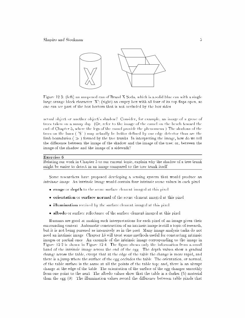
Label the line segments shown in Figure 12.3: an unopened can of brand X soda and anopen and empty box are lying on a table.
In Chapter 5 we studied methods of detecting contrast points in intensity images. Meth-ods of tracking and representing contours were given in Chapter 10. Unfortunately, several3D phenomena can cause the same kind of e�ect in the 2D image. For example, given a2D contour tracked in an intensity image, how do we decide if it is caused by viewing an
Shapiro and Stockman 5
Figure 12.3: (left) an unopened can of Brand X Soda, which is a solid blue can with a singlelarge orange block character 'X'; (right) an empty box with all four of its top aps open, soone can see part of the box bottom that is not occluded by the box sides.
actual object or another object's shadow? Consider, for example, an image of a grove oftrees taken on a sunny day. (Or, refer to the image of the camel on the beach toward theend of Chapter 5, where the legs of the camel provide the phenomena.) The shadows of thetrees on the lawn ( 'S' ) may actually be better de�ned by our edge detector than are thelimb boundaries ( � ) formed by the tree trunks. In interpreting the image, how do we tellthe di�erence between the image of the shadow and the image of the tree; or, between theimage of the shadow and the image of a sidewalk?
Exercise 6Relating our work in Chapter 5 to our current topic, explain why the shadow of a tree trunkmight be easier to detect in an image compared to the tree trunk itself.
Some researchers have proposed developing a sensing system that would produce anintrinsic image. An intrinsic image would contain four intrinsic scene values in each pixel.
� range or depth to the scene surface element imaged at this pixel
� orientation or surface normal of the scene element imaged at this pixel
� illumination received by the surface element imaged at this pixel
� albedo or surface re ectance of the surface element imaged at this pixel
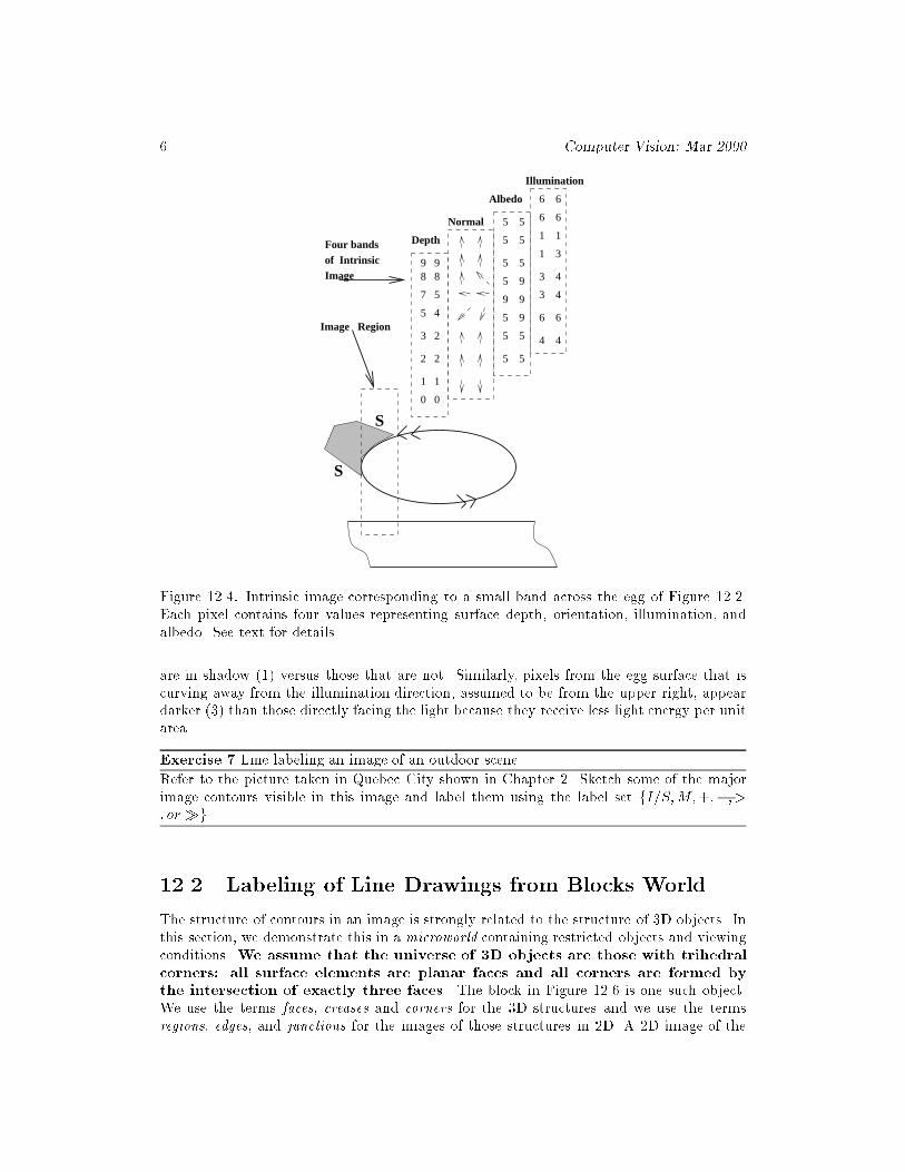
Humans are good at making such interpretations for each pixel of an image given theirsurrounding context. Automatic construction of an intrinsic image is still a topic of research,but it is not being pursued as intensively as in the past. Many image analysis tasks do notneed an intrinsic image. Chapter 13 will treat some methods useful for constucting intrinsicimages or partial ones. An example of the intrinsic image corresponding to the image inFigure 12.2 is shown in Figure 12.4. The �gure shows only the information from a smallband of the intrinsic image across the end of the egg. The depth values show a gradualchange across the table, except that at the edge of the table the change is more rapid, andthere is a jump where the surface of the egg occludes the table. The orientation, or normal,of the table surface is the same at all the points of the table top; and, there is an abruptchange at the edge of the table. The orientation of the surface of the egg changes smoothlyfrom one point to the next. The albedo values show that the table is a darker (5) materialthan the egg (9). The illumination values record the di�erence between table pixels that
6 Computer Vision: Mar 2000
S
S
7 5
5 4
2 2
Image Region
Four bandsof IntrinsicImage
Depth
Albedo
Illumination
3 4
3 4
1 3
1 1
6 6
6 6
5 5
5 5
5 5
5 9
9 9
5 9
5 5
5 5
9 9
1 1
0 0
8 8
6 6
4 4
Normal
3 2
Figure 12.4: Intrinsic image corresponding to a small band across the egg of Figure 12.2.Each pixel contains four values representing surface depth, orientation, illumination, andalbedo. See text for details.
are in shadow (1) versus those that are not. Similarly, pixels from the egg surface that iscurving away from the illumination direction, assumed to be from the upper right, appeardarker (3) than those directly facing the light because they receive less light energy per unitarea.
Exercise 7 Line labeling an image of an outdoor scene.
Refer to the picture taken in Quebec City shown in Chapter 2. Sketch some of the majorimage contours visible in this image and label them using the label set fI=S;M;+;�; >; or�g
12.2 Labeling of Line Drawings from Blocks World
The structure of contours in an image is strongly related to the structure of 3D objects. Inthis section, we demonstrate this in a microworld containing restricted objects and viewingconditions. We assume that the universe of 3D objects are those with trihedral
corners: all surface elements are planar faces and all corners are formed by
the intersection of exactly three faces. The block in Figure 12.6 is one such object.We use the terms faces, creases and corners for the 3D structures and we use the termsregions, edges, and junctions for the images of those structures in 2D. A 2D image of the
Shapiro and Stockman 7
+ + - -
+- -+
+ +-
++
+
- -
-
+ -
L-junctions
arrow junctions
fork junctions
T-junctions
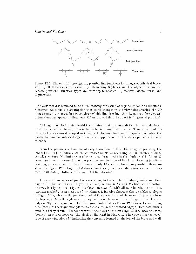
Figure 12.5: The only 16 topologically possible line junctions for images of trihedral blocksworld ( all 3D corners are formed by intersecting 3 planes and the object is viewed ingeneral position). Junction types are, from top to bottom, L-junctions, arrows, forks, andT-junctions.
3D blocks world is assumed to be a line drawing consisting of regions, edges, and junctions.Moreover, we make the assumption that small changes in the viewpoint creating the 2Dimage cause no changes in the topology of this line drawing; that is, no new faces, edges,or junctions can appear or disappear. Often it is said that the object is \in general position".
Although our blocks microworld is so limited that it is unrealistic, the methods devel-oped in this context have proven to be useful in many real domains. Thus we will add tothe set of algorithms developed in Chapter 11 for matching and interpretation. Also, theblocks domain has historical signi�cance and supports an intuitive development of the newmethods.
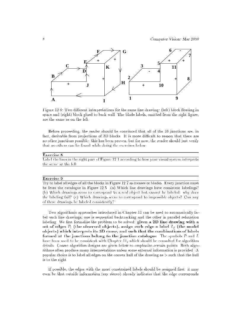
From the previous section, we already know how to label the image edges using thelabels f+;�; >g to indicate which are creases or blades according to our interpretation ofthe 3D structure. No limbs are used since they do not exist in the blocks world. About 30years ago, it was discovered that the possible combinations of line labels forming junctionsis strongly constrained. In total, there are only 16 such combinations possible: these areshown in Figure 12.5. Figure 12.6 shows how these junction con�gurations appear in twodistinct 3D interpretations of the same 2D line drawing.
There are four types of junctions according to the number of edges joining and theirangles: for obvious reasons, they're called L's, arrows, forks, and T's from top to bottomby rows in Figure 12.5. Figure 12.6 shows an example with all four junction types. Thejunction marked J is an instance of the leftmost L-junction shown at the top of the cataloguein Figure 12.5, whereas the junction marked C is an instance of the second L-junction fromthe top right. G is the rightmost arrow-junction in the second row of Figure 12.5. There isonly one T-junction, markedD in the �gure. Note that, as Figure 12.5 shows, the occludingedge (cross) of the T-junction places no constraint on the occluded edge; all four possibilitiesremain, as they should. The four arrows in the block at the left (B,E,G,I) all have the same(convex) structure; however, the block at the right in Figure 12.6 has one other (concave)type of arrow-junction (7), indicating the convexity formed by the join of the block and wall.
8 Computer Vision: Mar 2000
++
+ +
-
-
A
B
CD
E
F G
H
I
J
K
1
2
34
5
67
8
9
10
11
+
+
+
+
Figure 12.6: Two di�erent interpretations for the same line drawing: (left) block oating inspace and (right) block glued to back wall. The blade labels, omitted from the right �gure,are the same as on the left.
Before proceeding, the reader should be convinced that all of the 16 junctions are, infact, derivable from projections of 3D blocks. It is more di�cult to reason that there areno other junctions possible: this has been proven, but for now, the reader should just verifythat no others can be found while doing the exercises below.
Exercise 8Label the lines in the right part of Figure 12.1 according to how your visual system interpretsthe scene at the left.
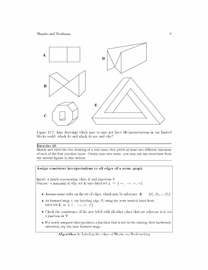
Exercise 9Try to label all edges of all the blocks in Figure 12.7 as creases or blades. Every junction mustbe from the catalogue in Figure 12.5. (a) Which line drawings have consistent labelings?(b) Which drawings seem to correspond to a real object but cannot be labeled: why doesthe labeling fail? (c) Which drawings seem to correspond to impossible objects? Can anyof these drawings be labeled consistently?
Two algorithmic approaches introduced in Chapter 11 can be used to automatically la-bel such line drawings; one is sequential backtracking and the other is parallel relaxationlabeling. We �rst formalize the problem to be solved: given a 2D line drawing with a
set of edges Pi (the observed objects), assign each edge a label Lj (the model
objects) which interprets its 3D cause, and such that the combinations of labels
formed at the junctions belong to the junction catalogue. The symbols P and L
have been used to be consistent with Chapter 11, which should be consulted for algorithmdetails. Coarse algorithm designs are given below to emphasize certain points. Both algo-rithms often produce many interpretations unless some external information is provided. Apopular choice is to label all edges on the convex hull of the drawing as > such that the hullis to the right.
If possible, the edges with the most constrained labels should be assigned �rst: it mayeven be that outside information (say stereo) already indicates that the edge corresponds
Shapiro and Stockman 9
A
B
C
D
E
Figure 12.7: Line drawings which may or may not have 3D interpetations in our limitedblocks world: which do and which do not and why?
Exercise 10Sketch and label the line drawing of a real scene that yields at least two di�erent instancesof each of the four junction types. Create your own scene: you may use any structures fromthe several �gures in this section.
Assign consistent interpretations to all edges of a scene graph.
Input: a graph representing edges E and junctions V.Output: a mapping of edge set E onto label set L = f + ; � ; >; <g.
� Assume some order on the set of edges, which may be arbitrary: E = fP1; P2; :::; Png.
� At forward stage i, try labeling edge Pi using the next untried label fromlabel set L = f + ; � ; >; <g.
� Check the consistency of the new label with all other edges that are adjacent to it viaa junction in V.
� If a newly assigned label produces a junction that is not in the catalog, then backtrack;otherwise, try the next forward stage.
Algorithm 1: Labeling the edges of Blocks via Backtracking
10 Computer Vision: Mar 2000
( B , ( B , ( B , + + - -+ +-
) ) )
A
B
C
D
( D, ( D, ( D,+-
-+
-+ ) ) )
( A, L )
++
of edge DB
L =
not in catalogue
IT
conflicting interpretation+ +
- - -+ +
( A, L )-
+L =
( A, )-
( C, )-
- -
A
B
C
D
not in catalogue
pryramid gluedto wall
Original LineDrawing
+
+
+
pryamid restingon table
pyramidfloating in air
--
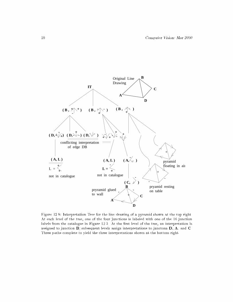
Figure 12.8: Interpretation Tree for the line drawing of a pyramid shown at the top right.At each level of the tree, one of the four junctions is labeled with one of the 16 junctionlabels from the catalogue in Figure 12.5. At the �rst level of the tree, an interpretation isassigned to junction B; subsequent levels assign interpretations to junctons D, A, and C.Three paths complete to yield the three interpretations shown at the bottom right.

Shapiro and Stockman 11
to a 3D crease, for example. Some preprocessing should be done to determine the type ofeach junction according to the angles and number of incident edges. Other versions of thisapproach assign catalog interpretations to the junction labels and proceed to eliminate thosethat are inconsistent across an edge with the neighboring junction interpetations. Figure12.8 shows an interpretation tree for interpreting the line drawing of a pyramid with fourfaces. The search space is rather small, demonstrating the strong constraints in trihedralblocks world.
Exercise 11Complete the IT shown in Figure 12.8 by providing all the edges and nodes omitted fromthe right side of the tree.
Exercise 12Construct the 5-level IT to assign consistent labels to all the edges of the pyramid shownin Figure 12.8. First, express the problem using the consistent labeling formalism fromChapter 11; de�ne P; L; RP ; RL, using the 5 observed edges and the 4 possible edgelabels. Secondly, sketch the IT. Are there three completed paths corresponding to the threecompleted paths in Figure 12.8?
12 Computer Vision: Mar 2000
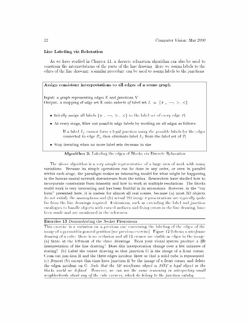
Line Labeling via Relaxation
As we have studied in Chapter 11, a discrete relaxation algorithm can also be used toconstrain the interpretations of the parts of the line drawing. Here we assign labels to theedges of the line drawing: a similar procedure can be used to assign labels to the junctions.
Assign consistent interpretations to all edges of a scene graph.
Input: a graph representing edges E and junctions V.Output: a mapping of edge set E onto subsets of label set L = f+ ; � ; >; <g.
� Initally assign all labels f+ ; � ; > ; <g to the label set of every edge Pi.
� At every stage, �lter out possible edge labels by working on all edges as follows:
{ If a label Lj cannot form a legal junction using the possible labels for the edgesconnected to edge Pi, then eliminate label Lj from the label set of Pi.
� Stop iterating when no more label sets decrease in size.
Algorithm 2: Labeling the edges of Blocks via Discrete Relaxation
The above algorithm is a very simple representative of a large area of work with manyvariations. Because its simple operations can be done in any order, or even in parallelwithin each stage, the paradigm makes an interesting model for what might be happeningin the human neural network downstream from the retina. Researchers have studied how toincorporate constraints from intensity and how to work at multiple resolutions. The blocksworld work is very interesting and has been fruitful in its extensions. However, in the \toyform" presented here, it is useless for almost all real scenes, because (a) most 3D objectsdo not satisfy the assumptions and (b) actual 2D image representations are typically quitefar from the line drawings required. Extensions, such as extending the label and junctioncatalogues to handle objects with curved surfaces and �xing errors in the line drawing, havebeen made and are mentioned in the references.
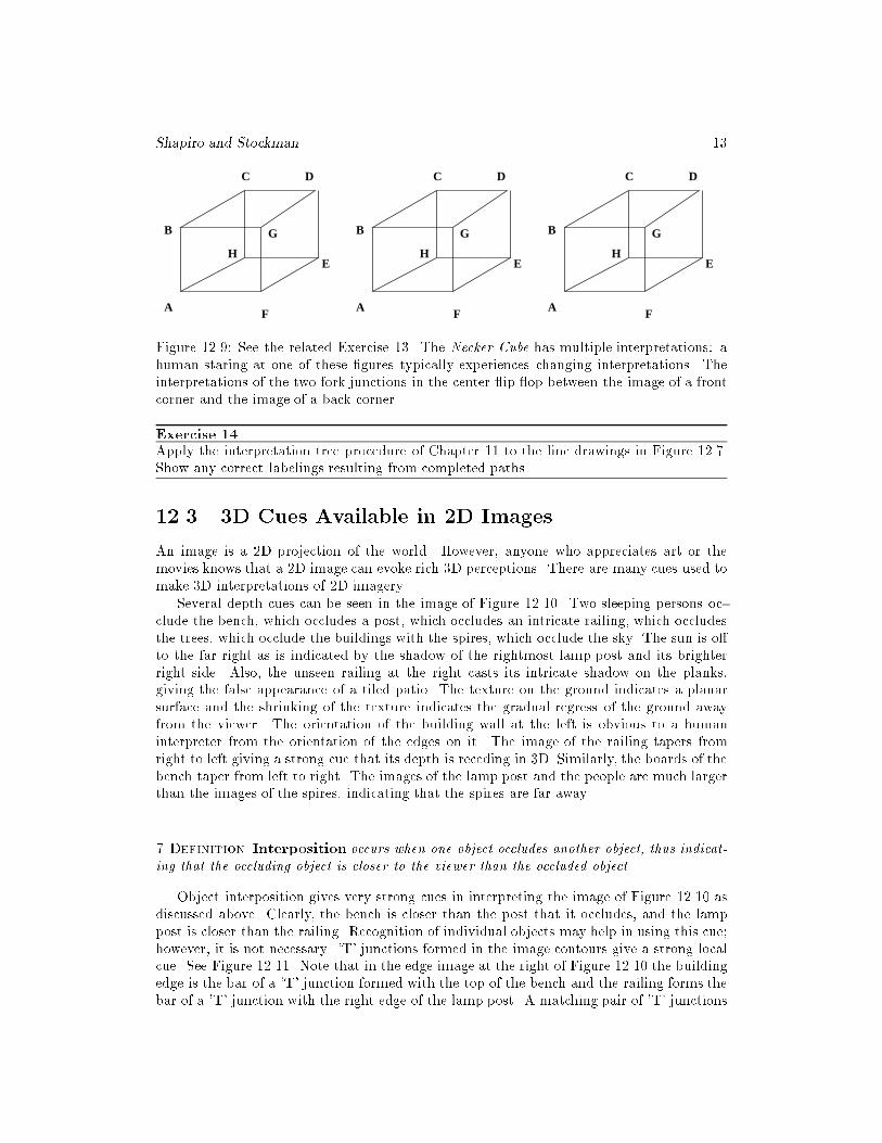
Exercise 13 Demonstrating the Necker Phenomena
This exercise is a variation on a previous one concerning the labeling of the edges of theimage of a pyramid in general position (see previous exercise). Figure 12.9 shows a wireframe
drawing of a cube: there is no occlusion and all 12 creases are visible as edges in the image.(a) Stare at the leftmost of the three drawings. Does your visual system produce a 3Dinterpretation of the line drawing? Does this interpretation change over a few minutes ofstaring? (b) Label the center drawing so that junction G is the image of a front corner.Cross out junction H and the three edges incident there so that a solid cube is represented.(c) Repeat (b) except this time have junction H be the image of a front corner and deletethe edges incident on G. Note that the 3D wireframe object is NOT a legal object in the
blocks world we de�ned. However, we can use the same reasoning in interpreting small
neighborhoods about any of the cube corners, which do belong to the junction catalog.
Shapiro and Stockman 13
A
B
C D
E
F
H
G
A
B
C D
E
F
H
G
A
B
C D
E
F
H
G
Figure 12.9: See the related Exercise 13. The Necker Cube has multiple interpretations: ahuman staring at one of these �gures typically experiences changing interpretations. Theinterpretations of the two fork junctions in the center ip op between the image of a frontcorner and the image of a back corner.
Exercise 14Apply the interpretation tree procedure of Chapter 11 to the line drawings in Figure 12.7.Show any correct labelings resulting from completed paths.
12.3 3D Cues Available in 2D Images
An image is a 2D projection of the world. However, anyone who appreciates art or themovies knows that a 2D image can evoke rich 3D perceptions. There are many cues used tomake 3D interpretations of 2D imagery.
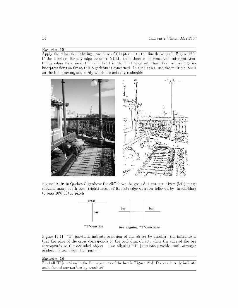
Several depth cues can be seen in the image of Figure 12.10. Two sleeping persons oc-clude the bench, which occludes a post, which occludes an intricate railing, which occludesthe trees, which occlude the buildings with the spires, which occlude the sky. The sun is o�to the far right as is indicated by the shadow of the rightmost lamp post and its brighterright side. Also, the unseen railing at the right casts its intricate shadow on the planks,giving the false appearance of a tiled patio. The texture on the ground indicates a planarsurface and the shrinking of the texture indicates the gradual regress of the ground awayfrom the viewer. The orientation of the building wall at the left is obvious to a humaninterpreter from the orientation of the edges on it. The image of the railing tapers fromright to left giving a strong cue that its depth is receding in 3D. Similarly, the boards of thebench taper from left to right. The images of the lamp post and the people are much largerthan the images of the spires, indicating that the spires are far away.
7 Definition Interposition occurs when one object occludes another object, thus indicat-
ing that the occluding object is closer to the viewer than the occluded object.
Object interposition gives very strong cues in interpreting the image of Figure 12.10 asdiscussed above. Clearly, the bench is closer than the post that it occludes, and the lamppost is closer than the railing. Recognition of individual objects may help in using this cue;however, it is not necessary. 'T' junctions formed in the image contours give a strong localcue. See Figure 12.11. Note that in the edge image at the right of Figure 12.10 the buildingedge is the bar of a 'T' junction formed with the top of the bench and the railing forms thebar of a 'T' junction with the right edge of the lamp post. A matching pair of 'T' junctions
14 Computer Vision: Mar 2000
Exercise 15Apply the relaxation labeling procedure of Chapter 11 to the line drawings in Figure 12.7.If the label set for any edge becomes NULL, then there is no consistent interpretation.If any edges have more than one label in the �nal label set, then there are ambiguousinterpretations as far as this algorithm is concerned. In such cases, use the multiple labelson the line drawing and verify which are actually realizable.
Figure 12.10: In Quebec City above the cli� above the great St Lawrence River: (left) imageshowing many depth cues, (right) result of Roberts edge operator followed by thresholdingto pass 10% of the pixels.
barbarbar
cross
"T"-junction two aligning "T"-junctions
Figure 12.11: \T"-junctions indicate occlusion of one object by another: the inference isthat the edge of the cross corresponds to the occluding object, while the edge of the barcorresponds to the occluded object. Two aligning \T"-junctions provide much strongerevidence of occlusion than just one.
Exercise 16
Find all 'T' junctions in the line segments of the box in Figure 12.3. Does each truly indicateocclusion of one surface by another?
Shapiro and Stockman 15
is an even stronger cue because it indicates a continuing object passing behind another.This edge image is di�cult as is often the case with outdoor scenes: for simpler situations,consider the next exercise. Interposition of recognized objects or surfaces can be
used to compute the relative depth of these objects.
8 Definition Perspective scaling indicates that the distance to an object is inversely
proportional to its image size. The term \scaling" is reserved for comparing object dimen-
sions that are parallel to the image plane.
Once we recognize the spires in Figure 12.10, we know they are quite distant becausetheir image size is small. The vertical elements of the railing decrease in size as we see themrecede in distance from right to left. Similarly, when we look down from a tall building tothe street below, our height is indicated by how small the people and cars appear. The
size of an object recognized in the image can be used to compute the depth of
that object in 3D.
9 Definition Forshortening of an object's image is due to viewing the object at an acute
angle to its axis and gives another strong cue of how the 2D view relates to the 3D object.
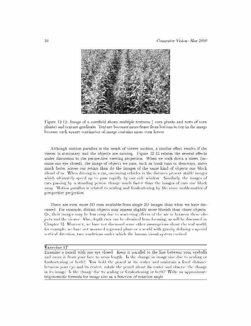
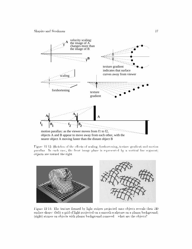
As we look at the bench in Figure 12.10 and the people on it, their image length is shorterthan it would be were the bench at a consistent closest distance to the viewer. Similarly,the verticle elements of the railing get closer together in the image as they get furtheraway in the scene. This forshortening would not occur were we to look perpendicularly atthe railing. Texture gradient is a related phenomena. Elements of a texture are subject toscaling and forshortening, so these changes give a viewer information about the distance andorientation of a surface containing texture. This e�ect is obvious when we look up at a brickbuilding, along a tiled oor or railroad track, or out over a �eld of corn or a stadium crowd.Figure 12.12 demonstrates this. Texture gradients also tell us something about the shapeof our friends' bodies when they wear clothes with regular textured patterns. A sketch of asimple situation creating a texture gradient is given in Figure 12.13: the texels, or imagesof the dots, move closer and closer together toward the center of the image correspondingto the increasing distance in 3D. Figure 12.14 shows how a texture is formed when objectsin a scene are illuminated by a regular grid of light stripes. This arti�cial (structured)lighting not only gives humans more information about the shape of the surfaces, but alsoallows automatic computation of surface normal or even depth as the next chapter will show.Change of texture in an image can be used to compute the orientation of the 3D surfaceyielding that texture.
10 Definition Texture gradient is the change of image texture (measured or perceived)
along some direction in the image, often corresponding to either a change in distance or
surface orientation in the 3D world containing the objects creating the texture.
Regular textured surfaces in 3D viewed nonfrontally create texture gradients in theimage, but the reverse may not be true. Certainly, artists create the illusion of 3D surfacesby creating texture gradients on a single 2D sheet of paper.
11 Definition Motion parallax gives a moving observer information about the depth to
objects, as even stationary objects appear to move relative to each other: the images of closer
objects will move faster than the images of distant objects.
16 Computer Vision: Mar 2000
Figure 12.12: Image of a corn�eld shows multiple textures ( corn plants and rows of cornplants) and texture gradients. Texture becomes more dense from bottom to top in the imagebecause each square centimeter of image contains more corn leaves.
Although motion parallax is the result of viewer motion, a similar e�ect results if theviewer is stationary and the objects are moving. Figure 12.13 relates the several e�ectsunder discussion to the perspective viewing projection. When we walk down a street (as-sume one eye closed), the image of objects we pass, such as trash cans or doorways, movemuch faster across our retina than do the images of the same kind of objects one blockahead of us. When driving in a car, oncoming vehicles in the distance present stable imageswhich ultimately speed up to pass rapidly by our side window. Similarly, the images ofcars passing by a standing person change much faster than the images of cars one blockaway. Motion parallax is related to scaling and forshortening by the same mathematics ofperspective projection.
There are even more 3D cues available from single 2D images than what we have dis-
cussed. For example, distant objects may appear slightly more blueish than closer objects.Or, their images may be less crisp due to scattering e�ects of the air in between these ob-jects and the viewer. Also, depth cues can be obtained from focusing, as will be discussed inChapter 13. Moreover, we have not discussed some other assumptions about the real world;for example, we have not assumed a ground plane or a world with gravity de�ning a specialvertical direction, two conditions under which the human visual system evolved.
Exercise 17
Examine a pencil with one eye closed. Keep it parallel to the line between your eyeballsand move it from your face to arms length. Is the change in image size due to scaling orforshortening or both? Now hold the pencil at its center and maintain a �xed distancebetween your eye and its center: rotate the pencil about its center and observe the changein its image. Is the change due to scaling or forshortening or both? Write an approximatetrigonometic formula for image size as a function of rotation angle.
Shapiro and Stockman 17
f1 f2 B
A
B B1 2
A A1 2
A
B
forshortening
scaling
velocity scaling:the image of Achanges more thanthe image of B
texturegradient
motion parallax: as the viewer moves from f1 to f2,objects A and B appear to move away from each other, with thenearer object A moving faster than the distant object B
texture gradientindicates that surfacecurves away from viewer
Figure 12.13: Sketches of the e�ects of scaling, forshortening, texture gradient and motionparallax. In each case, the front image plane is represented by a vertical line segment;objects are toward the right.
Figure 12.14: The texture formed by light stripes projected onto objects reveals their 3Dsurface shape: (left) a grid of light projected on a smooth sculpture on a planar background;(right) stripes on objects with planar background removed { what are the objects?
18 Computer Vision: Mar 2000
Exercise 18Hold a �nger vertically closely in front of your nose and alternately open one eye only for 2seconds. Observe the apparent motion of your �nger (which should not be moving). Moveyour �nger further away and repeat. Move your �nger to arms length and repeat again. (Itmight help to line up your �nger tip with a door knob or other object much farther away.)Describe the amount of apparent motion relative to the distance of �nger to nose.
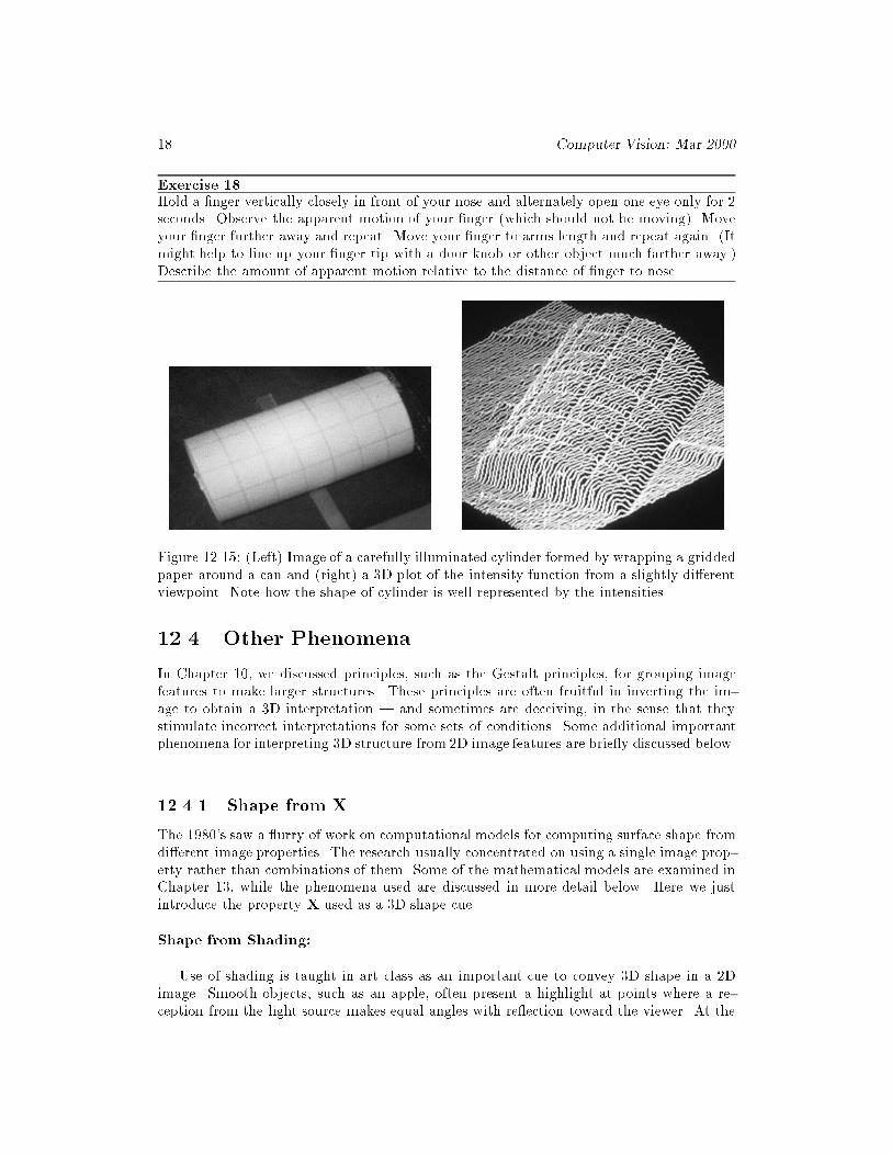
Figure 12.15: (Left) Image of a carefully illuminated cylinder formed by wrapping a griddedpaper around a can and (right) a 3D plot of the intensity function from a slightly di�erentviewpoint. Note how the shape of cylinder is well represented by the intensities.
12.4 Other Phenomena
In Chapter 10, we discussed principles, such as the Gestalt principles, for grouping imagefeatures to make larger structures. These principles are often fruitful in inverting the im-age to obtain a 3D interpretation | and sometimes are deceiving, in the sense that theystimulate incorrect interpretations for some sets of conditions. Some additional importantphenomena for interpreting 3D structure from 2D image features are brie y discussed below.
12.4.1 Shape from X
The 1980's saw a urry of work on computational models for computing surface shape fromdi�erent image properties. The research usually concentrated on using a single image prop-erty rather than combinations of them. Some of the mathematical models are examined inChapter 13, while the phenomena used are discussed in more detail below. Here we justintroduce the property X used as a 3D shape cue.
Shape from Shading:
Use of shading is taught in art class as an important cue to convey 3D shape in a 2Dimage. Smooth objects, such as an apple, often present a highlight at points where a re-ception from the light source makes equal angles with re ection toward the viewer. At the
Shapiro and Stockman 19
0
50
100
150
200
250
0 50 100 150 200 250
’egg-vaseR100’
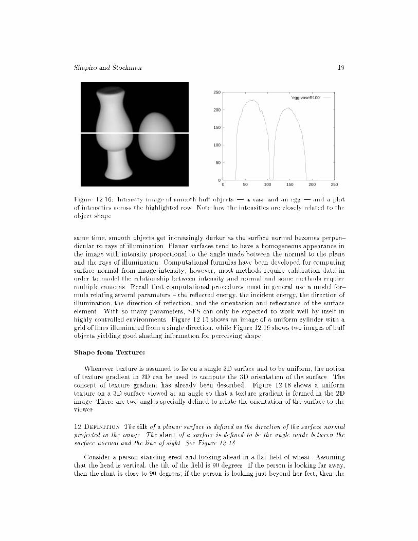
Figure 12.16: Intensity image of smooth bu� objects | a vase and an egg | and a plotof intensities across the highlighted row. Note how the intensities are closely related to theobject shape.
same time, smooth objects get increasingly darker as the surface normal becomes perpen-dicular to rays of illumination. Planar surfaces tend to have a homogeneous appearance inthe image with intensity proportional to the angle made between the normal to the planeand the rays of illumination. Computational formulas have been developed for computingsurface normal from image intensity; however, most methods require calibration data inorder to model the relationship between intensity and normal and some methods requiremultiple cameras. Recall that computational procedures must in general use a model for-mula relating several parameters { the re ected energy, the incident energy, the direction ofillumination, the direction of re ection, and the orientation and re ectance of the surfaceelement. With so many parameters, SFS can only be expected to work well by itself inhighly controlled environments. Figure 12.15 shows an image of a uniform cylinder with agrid of lines illuminated from a single direction, while Figure 12.16 shows two images of bu�objects yielding good shading information for perceiving shape.
Shape from Texture:
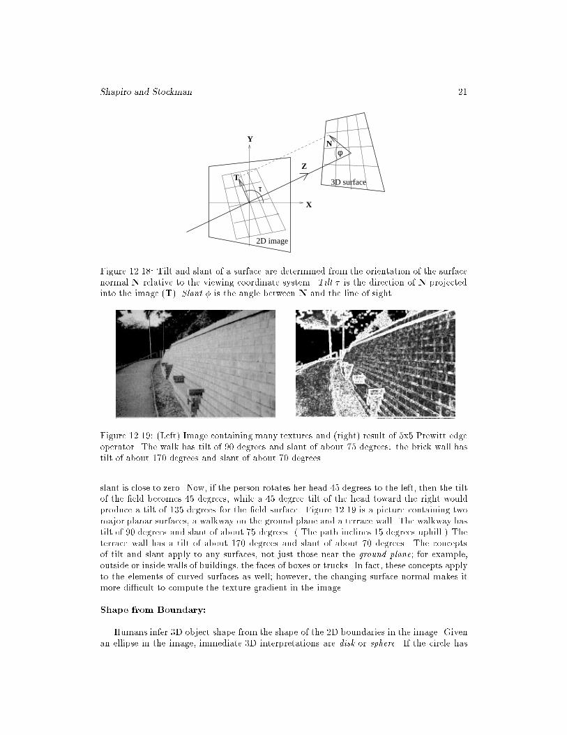
Whenever texture is assumed to lie on a single 3D surface and to be uniform, the notionof texture gradient in 2D can be used to compute the 3D orientation of the surface. Theconcept of texture gradient has already been described. Figure 12.18 shows a uniformtexture on a 3D surface viewed at an angle so that a texture gradient is formed in the 2Dimage. There are two angles specially de�ned to relate the orientation of the surface to theviewer.
12 Definition The tilt of a planar surface is de�ned as the direction of the surface normal
projected in the image. The slant of a surface is de�ned to be the angle made between the
surface normal and the line of sight. See Figure 12.18
Consider a person standing erect and looking ahead in a at �eld of wheat. Assumingthat the head is vertical, the tilt of the �eld is 90 degrees. If the person is looking far away,then the slant is close to 90 degrees; if the person is looking just beyond her feet, then the
20 Computer Vision: Mar 2000
�������������������������
�������������������������
������������������
������������������
������������������
������������������
�����������������������������������
�����������������������������������
(a) (b)
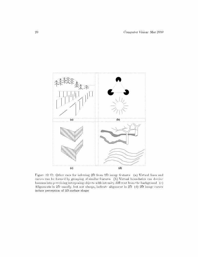
(c) (d)
Figure 12.17: Other cues for inferring 3D from 2D image features. (a) Virtual lines andcurves can be formed by grouping of similar features. (b) Virtual boundaries can deceivehumans into perceiving interposing objects with intensity di�erent from the background. (c)Alignments in 2D usually, but not always, indicate alignment in 3D. (d) 2D image curvesinduce perception of 3D surface shape.
Shapiro and Stockman 21
X
Y
ZT 3D surface
2D image
τ
Nφ
Figure 12.18: Tilt and slant of a surface are determined from the orientation of the surfacenormal N relative to the viewing coordinate system. Tilt � is the direction of N projectedinto the image (T). Slant � is the angle between N and the line of sight.
Figure 12.19: (Left) Image containing many textures and (right) result of 5x5 Prewitt edgeoperator. The walk has tilt of 90 degrees and slant of about 75 degrees: the brick wall hastilt of about 170 degrees and slant of about 70 degrees.
slant is close to zero. Now, if the person rotates her head 45 degrees to the left, then the tiltof the �eld becomes 45 degrees, while a 45 degree tilt of the head toward the right wouldproduce a tilt of 135 degrees for the �eld surface. Figure 12.19 is a picture containing twomajor planar surfaces, a walkway on the ground plane and a terrace wall. The walkway hastilt of 90 degrees and slant of about 75 degrees. ( The path inclines 15 degrees uphill.) Theterrace wall has a tilt of about 170 degrees and slant of about 70 degrees. The conceptsof tilt and slant apply to any surfaces, not just those near the ground plane; for example,outside or inside walls of buildings, the faces of boxes or trucks. In fact, these concepts applyto the elements of curved surfaces as well; however, the changing surface normal makes itmore di�cult to compute the texture gradient in the image.
Shape from Boundary:
Humans infer 3D object shape from the shape of the 2D boundaries in the image. Givenan ellipse in the image, immediate 3D interpretations are disk or sphere. If the circle has
22 Computer Vision: Mar 2000
Exercise 19
(a) Give the tilt and slant for each of the four faces of the object in Figure 12.6. (b) Do thesame for the faces of the objects in Figure 12.1.
uniform shading or texture the disk will be favored, if the shading or texture changes appro-priately toward the boundary, the sphere will be favored. Cartoons and other line drawingsoften have no shading or texture, yet humans can derive 3D shape descriptions from them.
Computational methods have been used to compute surface normals for points withina region enclosed by a smooth curve. Consider the simple case of a circle: the smoothnessassumption means that in 3D, the surface normals on the object limb are perpendicular toboth the line of sight and the circular cross section seen in the image. This allows us toassign a unique normal to the boundary points in the image. These normals are in oppositedirections for boundary points that are the endpoints of diameters of the circle. We canthen interpolate smooth changes to the surface normals across an entire diameter, makingsure that the middle pixel has a normal pointing right at the viewer. Surely, we need tomake an additional assumption to do this, because if we were looking at the end of an elipse,the surface would be di�erent from a sphere. Moreover, we could be looking at the inside
of a half spherical shell! Assumptions can be used to produce a unique surface, which maybe the wrong one. Shading information can be used to constrain the propagation of surfacenormals. Shading can di�erentiate between an egg and a ball, but maybe not between theoutside of a ball and the inside of a ball.
Exercise 20
Find a cartoon showing a smooth human or animal �gure. (a) Is there any shading, shadows,or texture to help with perception of 3D object shape? If not, add some yourself by assuminga light bulb at the front top right. (b) Trace the object boundary onto a clean sheet of paper.Assign surface normals to 20 or so points within the �gure boundary to represent the objectshape as it would be represented in an intrinsic image.
12.4.2 Vanishing Points
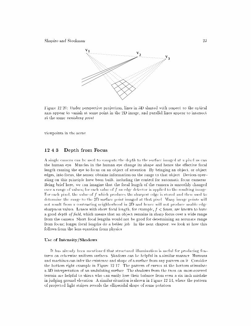
The perspective projection distorts parallel lines in interesting ways. Artists and draftsper-sons have used such knowledge in visual communication for centuries. Figure 12.20 showstwo well-known phenomena. First, a 3D line skew to the optical axis will appear to vanishat a point in the 2D image called the vanishing point. Secondly, a group of parallel lines willhave the same vanishing point as shown in the �gure. These e�ects are easy to show fromthe algebraic model of projective projection. Vanishing lines are formed by the vanishingpoints from di�erent groups of lines parallel to the same plane. In particular, a horizon
line is formed from the vanishing points of di�erent groups of parallel lines on the groundplane. In Figure 12.20, points V1 andV3 form a horizon for the ground plane formed by therectangular tiled surface. Note that the independent bundle of three parallel lines (highway)vanishes at point V2 which is on the same horizon line formed by the rectangular texture.Using these properties of perspective, camera models can be deduced from imagery takenfrom ordinary uncalibrated cameras. Recently, systems have been constructed using theseprinciples that can build 3D models of scenes from an ordinary video taken from several
Shapiro and Stockman 23
VV1
2 V3
Figure 12.20: Under perspective projection, lines in 3D slanted with respect to the opticalaxis appear to vanish at some point in the 2D image, and parallel lines appear to intersectat the same vanishing point.
viewpoints in the scene.
12.4.3 Depth from Focus
A single camera can be used to compute the depth to the surface imaged at a pixel as canthe human eye. Muscles in the human eye change its shape and hence the e�ective focallength causing the eye to focus on an object of attention. By bringing an object, or objectedges, into focus, the sensor obtains information on the range to that object. Devices oper-ating on this principle have been built, including the control for automatic focus cameras.Being brief here, we can imagine that the focal length of the camera is smoothly changedover a range of values; for each value of f an edge detector is applied to the resulting image.For each pixel, the value of f which produces the sharpest edge is stored and then used todetermine the range to the 3D surface point imaged at that pixel. Many image points willnot result from a contrasting neighborhood in 3D and hence will not produce usable edgesharpness values. Lenses with short focal length, for example, f < 8mm, are known to havea good depth of �eld, which means that an object remains in sharp focus over a wide rangefrom the camera. Short focal lengths would not be good for determining an accurate rangefrom focus; longer focal lengths do a better job. In the next chapter, we look at how thisfollows from the lens equation from physics.
Use of Intensity/Shadows
It has already been mentioned that structured illumination is useful for producing fea-tures on otherwise uniform surfaces. Shadows can be helpful in a similar manner. Humansand machines can infer the existence and shape of a surface from any pattern on it. Considerthe bottom right example in Figure 12.17. The pattern of curves at the bottom stimulatea 3D interpretation of an undulating surface. The shadows from the trees on snow-coveredterrain are helpful to skiers who can easily lose their balance from even a six inch mistakein judging ground elevation. A similar situation is shown in Figure 12.14, where the patternof projected light stripes reveals the ellipsoidal shape of some potatoes.
24 Computer Vision: Mar 2000
12.4.4 Motion Phenomena
Motion parallax has already been considered. When a moving visual sensor pursues anobject in 3D, points on that object appear to expand in the 2D image as the sensor closes inon the object. (Points on that object would appear to contract, not expand, if that objectwere escaping faster than the pursuer.) The point which is the center of pursuit is calledthe focus of expansion. The same phenomena results if the object moves toward the sensor:in this case, the rapid expansion of the object image is called looming. Chapter 9 treatedthese ideas in terms of optical ow. Quantitative methods exist to relate the image ow tothe distance and speed of the objects or pursuer.
12.4.5 Boundaries and Virtual Lines
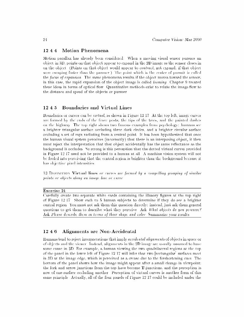
Boundaries or curves can be virtual, as shown in Figure 12.17. At the top left, image curvesare formed by the ends of the fence posts, the tips of the trees, and the painted dasheson the highway. The top right shows two famous examples from psychology: humans seea brighter triangular surface occluding three dark circles, and a brighter circular surfaceoccluding a set of rays radiating from a central point. It has been hypothesized that oncethe human visual system perceives (incorrectly) that there is an interposing object, it thenmust reject the interpretation that that object accidentally has the same re ectance as thebackground it occludes. So strong is this perception that the dotted virtual curves providedin Figure 12.17 need not be provided to a human at all. A machine vision system will notbe fooled into perceiving that the central region is brighter than the background because ithas objective pixel intensities.
13 Definition Virtual lines or curves are formed by a compelling grouping of similar
points or objects along an image line or curve.
Exercise 21Carefully create two separate white cards containing the illusory �gures at the top rightof Figure 12.17. Show each to 5 human subjects to determine if they do see a brightercentral region. You must not ask them this question directly: instead, just ask them generalquestions to get them to describe what they perceive. Ask What objects do you perceive?
Ask Please describe them in terms of their shape and color. Summarize your results.
12.4.6 Alignments are Non-Accidental
Humans tend to reject interpretations that imply accidental alignments of objects in space orof objects and the viewer. Instead, alignments in the 2D image are usually assumed to havesome cause in 3D. For example, a human viewing the two quadrilateral regions at the topof the panel in the lower left of Figure 12.17 will infer that two [rectangular] surfaces meetin 3D at the image edge, which is perceived as a crease due to the forshortening cues. Thebottom of the panel shows how the image might appear after a small change in viewpoint:the fork and arrow junctions from the top have become T-junctions, and the perception isnow of one surface occluding another. Perception of virtual curves is another form of thissame principle. Actually, all of the four panels of Figure 12.17 could be included under the
Shapiro and Stockman 25
same principle. As proposed in Irving Rock's 1983 treatise, the human visual system seemsto accept the simplest hypothesis that explains the image data. (This viewpoint explainsmany experiments and makes vision similar to reasoning. However, it also seems to contra-dict some experimental data and may make vision programming very di�cult.)
Some of the heuristics that have been proposed for image interpretation follow. None ofthese give correct interpretations in all cases: counterexamples are easy to �nd. We use theterm edge here also to mean crease, mark, or shadow in 3D in addition to its 2D meaning.
� From a straight edge in the image, infer a straight edge in 3D.
� From edges forming a junction in the 2D image, infer edges forming a corner in 3D.(More generally, from coincidence in 2D infer coincidence in 3D.)
� From similar objects on a curve in 2D, infer similar objects on a curve in 3D.
� From a 2D polygonal region, infer a polygonal face in 3D.
� From a smooth curved boundary in 2D, infer a smooth object in 3D.
� Symmetric regions in 2D correspond to symmetric objects in 3D.
12.5 The Perspective Imaging Model
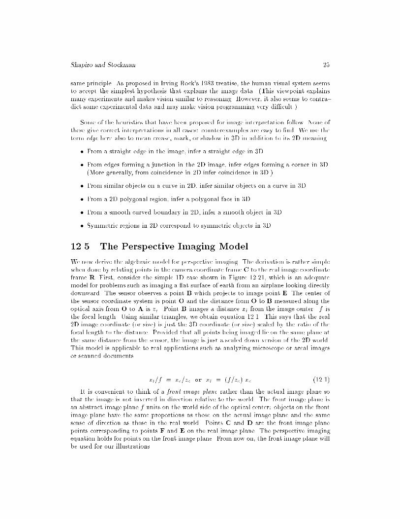
We now derive the algebraic model for perspective imaging. The derivation is rather simplewhen done by relating points in the camera coordinate frameC to the real image coordinateframe R. First, consider the simple 1D case shown in Figure 12.21, which is an adequatemodel for problems such as imaging a at surface of earth from an airplane looking directlydownward. The sensor observes a point B which projects to image point E. The center ofthe sensor coordinate system is point O and the distance from O to B measured along theoptical axis from O to A is zc. Point B images a distance xi from the image center. f isthe focal length. Using similar triangles, we obtain equation 12.1. This says that the real2D image coordinate (or size) is just the 3D coordinate (or size) scaled by the ratio of thefocal length to the distance. Provided that all points being imaged lie on the same plane at
the same distance from the sensor, the image is just a scaled down version of the 2D world.This model is applicable to real applications such as analyzing microscope or areal imagesor scanned documents.
xi=f = xc=zc or xi = (f=zc) xc (12.1)
It is convenient to think of a front image plane rather than the actual image plane sothat the image is not inverted in direction relative to the world. The front image plane isan abstract image plane f units on the world side of the optical center: objects on the frontimage plane have the same proportions as those on the actual image plane and the samesense of direction as those in the real world. Points C and D are the front image planepoints corresponding to points F and E on the real image plane. The perspective imagingequation holds for points on the front image plane. From now on, the front image plane willbe used for our illustrations.
26 Computer Vision: Mar 2000
x
f
zc
Xc
xf
D
A B
E F
fC
i
xc
Xi
Zc
real image plane
lens center O
Xf front image plane
camera and worldX-axis
. .
. .
..
O
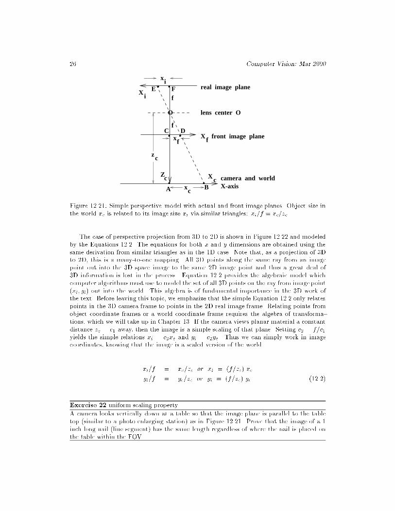
Figure 12.21: Simple perspective model with actual and front image planes. Object size inthe world xc is related to its image size xi via similar triangles: xi=f = xc=zc.
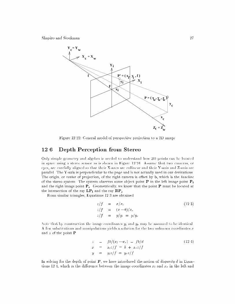
The case of perspective projection from 3D to 2D is shown in Figure 12.22 and modeledby the Equations 12.2. The equations for both x and y dimensions are obtained using thesame derivation from similar triangles as in the 1D case. Note that, as a projection of 3Dto 2D, this is a many-to-one mapping. All 3D points along the same ray from an imagepoint out into the 3D space image to the same 2D image point and thus a great deal of3D information is lost in the process. Equation 12.2 provides the algebraic model whichcomputer algorithms must use to model the set of all 3D points on the ray from image point(xi; yi) out into the world. This algebra is of fundamental importance in the 3D work ofthe text. Before leaving this topic, we emphasize that the simple Equation 12.2 only relatespoints in the 3D camera frame to points in the 2D real image frame. Relating points fromobject coordinate frames or a world coordinate frame requires the algebra of transforma-tions, which we will take up in Chapter 13. If the camera views planar material a constantdistance zc = c1 away, then the image is a simple scaling of that plane. Setting c2 = f=c1yields the simple relations xi = c2xc and yi = c2yc. Thus we can simply work in imagecoordinates, knowing that the image is a scaled version of the world.
xi=f = xc=zc or xi = (f=zc) xc
yi=f = yc=zc or yi = (f=zc) yc (12.2)
Exercise 22 uniform scaling property
A camera looks vertically down at a table so that the image plane is parallel to the tabletop (similar to a photo enlarging station) as in Figure 12.21. Prove that the image of a 1inch long nail (line segment) has the same length regardless of where the nail is placed onthe table within the FOV.
Shapiro and Stockman 27
Xc
Yc
xc
yc
yi
xi
P’ = ( x , y , f )
F
f
Yi
Xi
= Xw
= Yw
i i
P = ( x , y , z )w w w
= ZwZc
Figure 12.22: General model of perspective projection to a 2D image.
12.6 Depth Perception from Stereo
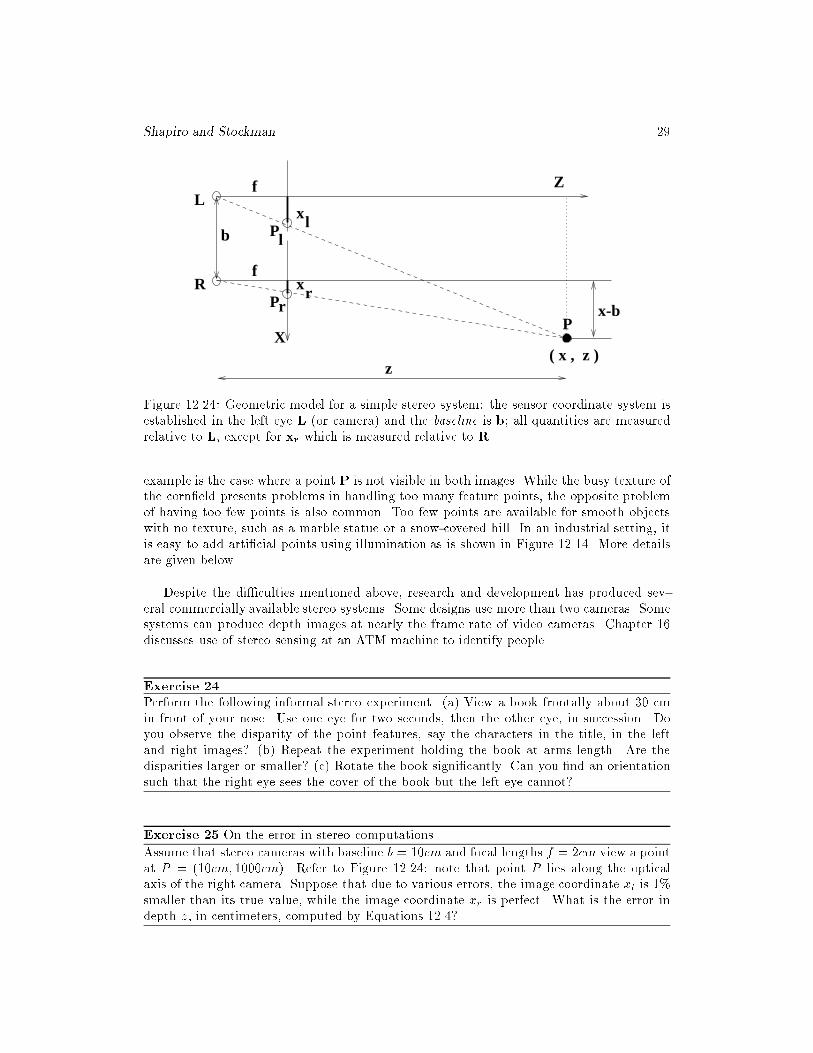
Only simple geometry and algebra is needed to understand how 3D points can be locatedin space using a stereo sensor as is shown in Figure 12.24. Assume that two cameras, oreyes, are carefully aligned so that their X-axes are collinear and their Y-axis and Z-axis areparallel. The Y-axis is perpendicular to the page and is not actually used in our derivations.The origin, or center of projection, of the right camera is o�set by b, which is the baselineof the stereo system. The system observes some object point P in the left image point Pl
and the right image point Pr. Geometrically, we know that the point P must be located atthe intersection of the ray LPl and the ray RPr.
From similar triangles, Equations 12.3 are obtained.
z=f = x=xl (12.3)
z=f = (x� b)=xr
z=f = y=yl = y=yr
Note that by construction the image coordinates yl and yr may be assumed to be identical.A few substitutions and manipulations yields a solution for the two unknown coordinates xand z of the point P.
z = fb=(xl � xr) = fb=d (12.4)
x = xlz=f = b + xrz=f
y = ylz=f = yrz=f
In solving for the depth of point P, we have introduced the notion of disparity d in Equa-tions 12.4, which is the di�erence between the image coordinates xl and xr in the left and
28 Computer Vision: Mar 2000
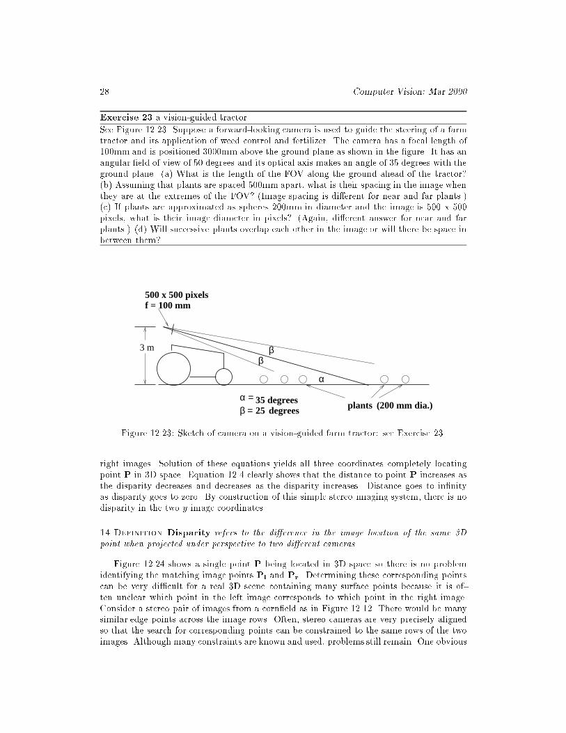
Exercise 23 a vision-guided tractor
See Figure 12.23. Suppose a forward-looking camera is used to guide the steering of a farmtractor and its application of weed control and fertilizer. The camera has a focal length of100mm and is positioned 3000mm above the ground plane as shown in the �gure. It has anangular �eld of view of 50 degrees and its optical axis makes an angle of 35 degrees with theground plane. (a) What is the length of the FOV along the ground ahead of the tractor?(b) Assuming that plants are spaced 500mm apart, what is their spacing in the image whenthey are at the extremes of the FOV? (Image spacing is di�erent for near and far plants.)(c) If plants are approximated as spheres 200mm in diameter and the image is 500 x 500pixels, what is their image diameter in pixels? (Again, di�erent answer for near and farplants.) (d) Will successive plants overlap each other in the image or will there be space inbetween them?
3 m
α
α =plants
ββ
degrees35 degrees
β = 25
f = 100 mm
(200 mm dia.)
500 x 500 pixels
Figure 12.23: Sketch of camera on a vision-guided farm tractor: see Exercise 23.
right images. Solution of these equations yields all three coordinates completely locatingpoint P in 3D space. Equation 12.4 clearly shows that the distance to point P increases asthe disparity decreases and decreases as the disparity increases. Distance goes to in�nityas disparity goes to zero. By construction of this simple stereo imaging system, there is nodisparity in the two y image coordinates.
14 Definition Disparity refers to the di�erence in the image location of the same 3D
point when projected under perspective to two di�erent cameras.
Figure 12.24 shows a single point P being located in 3D space so there is no problemidentifying the matching image points Pl and Pr. Determining these corresponding pointscan be very di�cult for a real 3D scene containing many surface points because it is of-ten unclear which point in the left image corresponds to which point in the right image.Consider a stereo pair of images from a corn�eld as in Figure 12.12. There would be manysimilar edge points across the image rows. Often, stereo cameras are very precisely alignedso that the search for corresponding points can be constrained to the same rows of the twoimages. Although many constraints are known and used, problems still remain. One obvious
Shapiro and Stockman 29
��������
f
f
L
R
X
Z
( x , z )
bx
xr
l
x-b
Pl
Pr
z
P
Figure 12.24: Geometric model for a simple stereo system: the sensor coordinate system isestablished in the left eye L (or camera) and the baseline is b; all quantities are measuredrelative to L, except for xr which is measured relative to R.
example is the case where a point P is not visible in both images. While the busy texture ofthe corn�eld presents problems in handling too many feature points, the opposite problemof having too few points is also common. Too few points are available for smooth objectswith no texture, such as a marble statue or a snow-covered hill. In an industrial setting, itis easy to add arti�cial points using illumination as is shown in Figure 12.14. More detailsare given below.
Despite the di�culties mentioned above, research and development has produced sev-eral commercially available stereo systems. Some designs use more than two cameras. Somesystems can produce depth images at nearly the frame rate of video cameras. Chapter 16discusses use of stereo sensing at an ATM machine to identify people.
Exercise 24
Perform the following informal stereo experiment. (a) View a book frontally about 30 cmin front of your nose. Use one eye for two seconds, then the other eye, in succession. Doyou observe the disparity of the point features, say the characters in the title, in the leftand right images? (b) Repeat the experiment holding the book at arms length. Are thedisparities larger or smaller? (c) Rotate the book signi�cantly. Can you �nd an orientationsuch that the right eye sees the cover of the book but the left eye cannot?
Exercise 25 On the error in stereo computations
Assume that stereo cameras with baseline b = 10cm and focal lengths f = 2cm view a pointat P = (10cm; 1000cm). Refer to Figure 12.24: note that point P lies along the opticalaxis of the right camera. Suppose that due to various errors, the image coordinate xl is 1%smaller than its true value, while the image coordinate xr is perfect. What is the error indepth z, in centimeters, computed by Equations 12.4?
30 Computer Vision: Mar 2000
Stereo Displays
Stereo displays are generated by computer graphics systems in order to convey 3D shapeto an interactive user. The graphics problem is the inverse of the computer vision problem:all the 3D surface points (x; y; z) are known and the system must create the left and rightimages. By rearranging the Equations 12.4 we arrive at Equations 12.5, which give formulasfor computing image coordinates (xl; yl) and (xr; yr) for a given object point (x; y; z) and�xed baseline b and focal length f . Thus, given a computer model of an object, the graphicssystem generates two separate images. These two images are presented to the user in oneof two ways: (a) one image is piped to the left eye and one is piped to the right eye using aspecial helmet or (b) the two images are presented alternately on a CRT using complimentarycolors which the user views with di�erent �lters on each eye. There is an inexpensive thirdmethod if motion is not needed: humans can actually fuse a stereo pair of images printedside-by-side on plain paper. (For example, stare at the stereogram that is Figure 7 of thepaper by Tanimoto (1998) cited in the references.)
xl = xf=z (12.5)
xr = f(x � b)=z
yl = yr = yf=z
Chapter 15 discusses in more detail how stereo displays are used in virtual reality systems,which engage users to an increased degree as a result of the 3D realism. Also, they can bevery useful in conveying to a radiologist the structure of 3D volumetric data from an MRIdevice.
12.6.1 Establishing Correspondences
The most di�cult part of a stereo vision system is not the depth calculation, but the deter-mination of the correspondences used in the depth calculation. If any correspondences areincorrect, they will produce incorrect depths, which can be just a little o� or totally wrong.In this section we discuss the major methods used for �nding correspondences and some
helpful constraints.
Cross Correlation
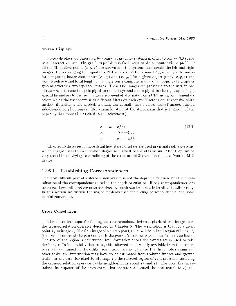
The oldest technique for �nding the correspondence between pixels of two images usesthe cross-correlation operator described in Chapter 5. The assumption is that for a givenpoint P1 in image I1 (the �rst image of a stereo pair), there will be a �xed region of image I2(the second image of the pair) in which the point P2 that corresponds to P1 must be found.The size of the region is determined by information about the camera setup used to takethe images. In industrial vision tasks, this information is readily available from the cameraparameters obtained by the calibration procedure (See Chapter 13). In remote sensing andother tasks, the information may have to be estimated from training images and groundtruth. In any case, for pixel P1 of image I1, the selected region of I2 is searched, applyingthe cross-correlation operator to the neighborhoods about P1 and P2. The pixel that max-imizes the response of the cross correlation operator is deemed the best match to P1 and
Shapiro and Stockman 31
Image I1 Image I2
Figure 12.25: The cross-correlation technique for �nding correspondences in a stereo pair ofimages.
used to �nd the depth at the corresponding 3D point. The cross-correlation technique hasbeen used very successfully to �nd correspondences in satellite and aerial imagery. Figure12.25 illustrates the cross-correlation technique. The black dot in image I1 indicates a pointwhose correspondence is sought. The square region in image I2 is the region to be searchedfor a match.
Symbolic Matching and Relational Constraints
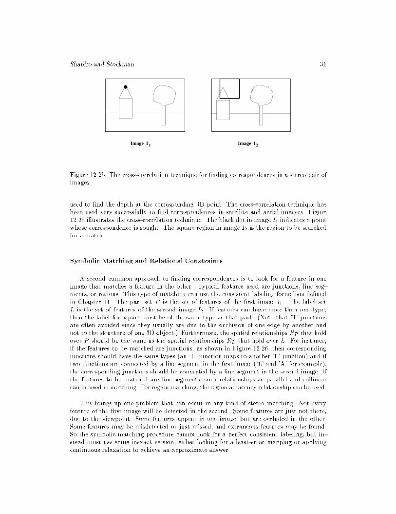
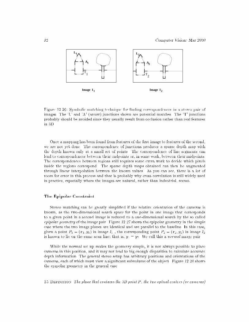
A second common approach to �nding correspondences is to look for a feature in oneimage that matches a feature in the other. Typical features used are junctions, line seg-ments, or regions. This type of matching can use the consistent labeling formalism de�nedin Chapter 11. The part set P is the set of features of the �rst image I1. The label setL is the set of features of the second image I2. If features can have more than one type,then the label for a part must be of the same type as that part. (Note that 'T' junctionsare often avoided since they usually are due to the occlusion of one edge by another andnot to the structure of one 3D object.) Furthermore, the spatial relationships RP that holdover P should be the same as the spatial relationships RL that hold over L. For instance,if the features to be matched are junctions, as shown in Figure 12.26, then correspondingjunctions should have the same types (an 'L' junction maps to another 'L' junction) and iftwo junctions are connected by a line segment in the �rst image ('L' and 'A' for example),the corresponding junctions should be connected by a line segment in the second image. Ifthe features to be matched are line segments, such relationships as parallel and collinearcan be used in matching. For region matching, the region adjacency relationship can be used.
This brings up one problem that can occur in any kind of stereo matching. Not everyfeature of the �rst image will be detected in the second. Some features are just not there,due to the viewpoint. Some features appear in one image, but are occluded in the other.Some features may be misdetected or just missed, and extraneous features may be found.So the symbolic matching procedure cannot look for a perfect consistent labeling, but in-stead must use some inexact version, either looking for a least-error mapping or applyingcontinuous relaxation to achieve an approximate answer.
32 Computer Vision: Mar 2000
Image I1 Image I2
LL1 2
AA1 2
T1 T
2
Figure 12.26: Symbolic matching technique for �nding correspondences in a stereo pair ofimages. The 'L' and 'A' (arrow) junctions shown are potential matches. The 'T' junctionsprobably should be avoided since they usually result from occlusion rather than real featuresin 3D.
Once a mapping has been found from features of the �rst image to features of the second,we are not yet done. The correspondence of junctions produces a sparse depth map withthe depth known only at a small set of points. The correspondence of line segments canlead to correspondences between their endpoints or, in some work, between their midpoints.The correspondences between regions still requires some extra work to decide which pixelsinside the regions correspond. The sparse depth maps obtained can then be augmentedthrough linear interpolation between the known values. As you can see, there is a lot ofroom for error in this process and that is probably why cross correlation is still widely usedin practice, especially where the images are natural, rather than industrial, scenes.
The Epipolar Constraint
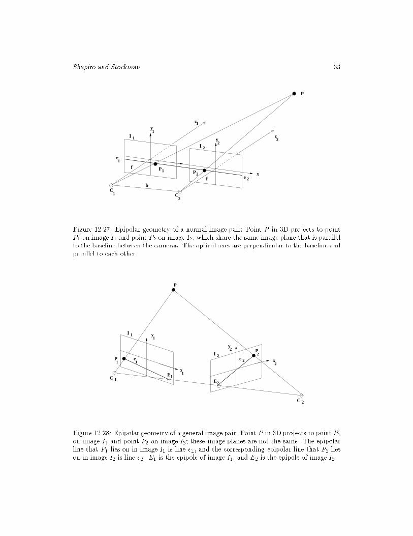
Stereo matching can be greatly simpli�ed if the relative orientation of the cameras isknown, as the two-dimensional search space for the point in one image that correspondsto a given point in a second image is reduced to a one-dimensional search by the so calledepipolar geometry of the image pair. Figure 12.27 shows the epipolar geometry in the simplecase where the two image planes are identical and are parallel to the baseline. In this case,given a point P1 = (x1; y1) in image I1 , the corresponding point P2 = (x2; y2) in image I2is known to lie on the same scan line; that is, y1 = y2. We call this a normal image pair.
While the normal set up makes the geometry simple, it is not always possible to placecameras in this position, and it may not lead to big enough disparities to calculate accuratedepth information. The general stereo setup has arbitrary positions and orientations of thecameras, each of which must view a signi�cant subvolume of the object. Figure 12.28 showsthe epipolar geometry in the general case.
15 Definition The plane that contains the 3D point P , the two optical centers (or cameras)
Shapiro and Stockman 33
C
bf
f
C
P
1
e1
e 2
z
z2
PP
y
y
x
2
2
21
1
1
2
1I
I
Figure 12.27: Epipolar geometry of a normal image pair: Point P in 3D projects to pointP1 on image I1 and point P2 on image I2, which share the same image plane that is parallelto the baseline between the cameras. The optical axes are perpendicular to the baseline andparallel to each other.
y
y
x
xP
P
P
e e1 2
2
1
1
2
1
2
EE2
1C
C
1
2
I
I
1
2
Figure 12.28: Epipolar geometry of a general image pair: Point P in 3D projects to point P1on image I1 and point P2 on image I2; these image planes are not the same. The epipolarline that P1 lies on in image I1 is line e1, and the corresponding epipolar line that P2 lieson in image I2 is line e2. E1 is the epipole of image I1, and E2 is the epipole of image I2.
34 Computer Vision: Mar 2000
C1 and C2, and the two image points P1 and P2 to which P projects is called the epipolar
plane.
16 Definition The two lines e1 and e2 resulting from the intersection of the epipolar plane
with the two image planes I1 and I2 are called epipolar lines.
Given the point P1 on epipolar line e1 in image I1 and knowing the relative orientationsof the cameras (see Ch 13), it is possible to �nd the corresponding epipolar line e2 in imageI2 on which the corresponding point P2 must lie. If another point P
0
1 in image I1 lies in adi�erent epipolar plane from point P1, it will lie on a di�erent epipolar line.
17 Definition The epipole of an image of a stereo pair is the point at which all its epipolar
lines intersect.
Points E1 and E2 are the epipoles of images I1 and I2, respectively.
The Ordering Constraint
Given a pair of points in the scene and their corresponding projections in each of the twoimages, the ordering constraint states that if these points lie on a continuous surface in thescene, they will be ordered in the same way along the epipolar lines in each of the images.This constraint is more of a heuristic than the epipolar constraint, because we don't knowat the time of matching whether or not two image points lie on the same 3D surface. Thusit can be helpful in �nding potential matches, but it may cause correspondence errors if itis strictly applied.
Error versus Coverage
In designing a stereo system, there is a tradeo� between scene coverage and error incomputing depth. When the baseline is short, small errors in location of image points P1and P2 will propagate to larger errors in the computed depth of the 3D point P as canbe inferred from the �gures. Increasing the baseline improves accuracy. However, as thecameras move further apart, it becomes more likely that image point correspondences arelost due to increased e�ects of occlusion. It has been proposed that an angle of �=4 betweenoptical axes is a good compromise.
12.7 * The Thin Lens Equation
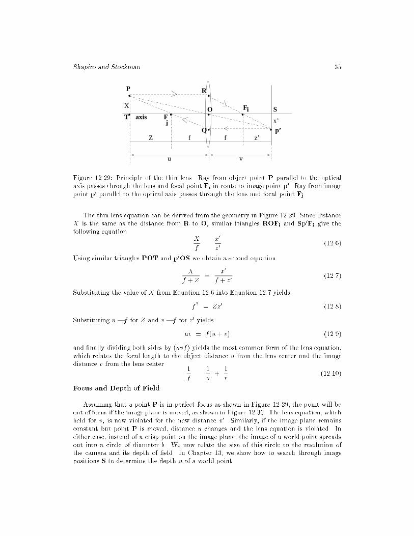
The principle of the thin lens equation is shown in Figure 12.29. A ray from object point Pparallel to the optical axis passes through the lens and focal point Fi in route to image pointp0. Other rays from P also reach p0 because the lens is a light collector. A ray through theoptical center O reaches p0 along a straight path. A ray from image point p0 parallel to theoptical axis passes through the lens and second focal point Fj.
Shapiro and Stockman 35
.
..
.
P
O ..
FiFj
axis
Q
R
p’
ST. .X
Z f f z’
x’
u v
Figure 12.29: Principle of the thin lens. Ray from object point P parallel to the opticalaxis passes through the lens and focal point Fi in route to image point p0. Ray from imagepoint p0 parallel to the optical axis passes through the lens and focal point Fj.
The thin lens equation can be derived from the geometry in Figure 12.29. Since distanceX is the same as the distance from R to O, similar triangles ROFi and Sp0Fi give thefollowing equation.
X
f=
x0
z0(12.6)
Using similar triangles POT and p0OS we obtain a second equation.
X
f + Z=
x0
f + z0(12.7)
Substituting the value of X from Equation 12.6 into Equation 12.7 yields
f2 = Zz0 (12.8)
Substituting u� f for Z and v � f for z0 yields
uv = f(u + v) (12.9)
and �nally dividing both sides by (uvf) yields the most common form of the lens equation,which relates the focal length to the object distance u from the lens center and the imagedistance v from the lens center.
1
f=
1
u+
1
v(12.10)
Focus and Depth of Field
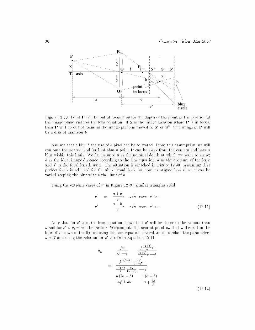
Assuming that a point P is in perfect focus as shown in Figure 12.29, the point will beout of focus if the image plane is moved, as shown in Figure 12.30. The lens equation, whichheld for v, is now violated for the new distance v0. Similarly, if the image plane remainsconstant but point P is moved, distance u changes and the lens equation is violated. Ineither case, instead of a crisp point on the image plane, the image of a world point spreadsout into a circle of diameter b. We now relate the size of this circle to the resolution ofthe camera and its depth of �eld. In Chapter 13, we show how to search through imagepositions S to determine the depth u of a world point.
36 Computer Vision: Mar 2000
.
.P
O ..
axisTS’
circle
pointin focus
Fi SS"
R
Q
blur
X
x’b
a2-
a-2
u v
v’
b
f
Figure 12.30: Point P will be out of focus if either the depth of the point or the position ofthe image plane violates the lens equation. If S is the image location where P is in focus,then P will be out of focus as the image plane is moved to S0 or S00. The image of P willbe a disk of diameter b.
Assume that a blur b the size of a pixel can be tolerated. From this assumption, we willcompute the nearest and farthest that a point P can be away from the camera and have ablur within this limit. We �x distance u as the nominal depth at which we want to sense;v as the ideal image distance according to the lens equation; a as the aperture of the lens;and f as the focal length used. The situation is sketched in Figure 12.30. Assuming thatperfect focus is achieved for the above conditions, we now investigate how much u can bevaried keeping the blur within the limit of b.
Using the extreme cases of v0 in Figure 12.30, similar triangles yield
v0 =a+ b
av : in case v0 > v
v0 =a� b
av : in case v0 < v (12.11)
Note that for v0 > v, the lens equation shows that u0 will be closer to the camera thanu and for v0 < v, u0 will be farther. We compute the nearest point un that will result in theblur of b shown in the �gure, using the lens equation several times to relate the parametersu; v; f and using the relation for v0 > v from Equation 12.11.
un =fv0
v0 � f=
f(a+b)
av
(a+b)
av � f
=f
(a+b)
a
uf
(u�f)
(a+b)
auf
(u�f)� f
=uf(a + b)
af + bu=
u(a+ b)
a + buf
(12.12)
Shapiro and Stockman 37
Similarly, by using v0 < v and the same steps given above, we obtain the location ur of thefar plane.
ur =uf(a � b)
af � bu=
u(a � b)
a� buf
(12.13)
18 Definition The depth of �eld is the di�erence between the far and near planes for
the given imaging parameters and limiting blur b.
Since u > f in typical situations, one can see from the �nal expression in Equation 12.12that un < u. Moreover, holding everything else constant, using a shorter focal length f willbring the near point closer to the camera. The same kind of argument shows that ur > u
and that shortening f will push the far point farther from the camera. Thus, shorter focallength lenses have a larger depth of �eld than lenses with longer focal lengths. (Unfortu-nately, shorter focal length lenses often have more radial distortion.)
Relating Resolution to Blur
A CCD camera with ideal optics can at best resolve n=2 distinct lines across n rows ofpixels, assuming that a spacing of one pixel between successive pairs of lines is necessary. A512�512 CCD array can detect a grid of 256 dark lines separated by one-pixel wide rows ofbright pixels. (If necessary, we can move the camera perpendicular to the optical axis slightlyuntil the line pattern aligns optimallywith the rows of pixels.) Blur larger than the pixel sizewill fuse all the lines into one grey image. The formulas given above enable one to engineerthe imaging equipment for a given detection problem. Once it is known what features mustbe detected and what stando� is practical, one can then decide on a detector array and lens.
19 Definition The resolving power of a camera is de�ned as Rp = 1=(2�) in units of
lines per inch (mm) where � is the pixel spacing in inches (mm).
For example, if a CCD array 10mm square has 500 � 500 pixels, the resolving poweris 1=(2 � 2 � 10�2mm=line) or 25 lines per mm. If we assume that black/white �lm iscomprised of silver halide molecules 5 � 10�3 mm apart, the resolving power is 100 linesper mm or 2500 lines per inch. The cones that sense color in the human eye are packeddensely in an area called the fovea, perhaps with a spacing of � = 10�4 inches. This trans-lates to a resolving power of 5 � 103 lines per inch on the retina. Using 20mm = 0:8inas the diameter of an eye, we can compute the subtended angle shown in Figure 12.31 as� � sin(�) = 2�=0:8in = 2:5� 10�4 radians, which is roughly one minute of arc. Thismeans that a human should be able to detect a line made by a 0.5 mm lead pencil on a wall2 meters away.
12.8 Concluding Discussion
This chapter examined a number of relations between 2D image structure and the surfacesand objects in the 3D world. Humans use many of these relations in combination to perceivethe world and to navigate within it. Although we only took a careful look at the relationshipof depth to stereo and focus, quantitative models have been formulated for many phenomena,
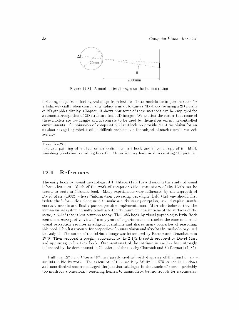
38 Computer Vision: Mar 2000
θ
∆
20mm
2000mm
Figure 12.31: A small object images on the human retina.
including shape from shading and shape from texture. These models are important tools forartists, especially when computer graphics is used, to convey 3D structure using a 2D canvasor 2D graphics display. Chapter 13 shows how some of these methods can be employed forautomatic recognition of 3D structure from 2D images. We caution the reader that some ofthese models are too fragile and inaccurate to be used by themselves except in controlledenvironments. Combination of computational methods to provide real-time vision for anoutdoor navigating robot is still a di�cult problem and the subject of much current researchactivity.
Exercise 26Locate a painting of a plaza or acropolis in an art book and make a copy of it. Markvanishing points and vanishing lines that the artist may have used in creating the picture.
12.9 References
The early book by visual psychologist J.J. Gibson (1950) is a classic in the study of visualinformation cues. Much of the work of computer vision researchers of the 1980s can betraced to roots in Gibson's book. Many experiments were in uenced by the approach ofDavid Marr (1982), whose \information processing paradigm" held that one should �rstisolate the information being used to make a decision or perception, second explore math-ematical models and �nally pursue possible implementations. Marr also believed that thehuman visual system actually constructed fairly complete descriptions of the surfaces of thescene, a belief that is less common today. The 1983 book by visual psychologist Irvin Rockcontains a retrospective view of many years of experiments and reaches the conclusion thatvisual perception requires intelligent operations and shares many properties of reasoning:this book is both a resource for properties of human vision and also for the methodology usedto study it. The notion of the intrinsic image was introduced by Barrow and Tenanbaum in1978. Their proposal is roughly equivalent to the 2 1/2 D sketch proposed by David Marrand appearing in his 1982 book. Our treatment of the intrinsic image has been stronglyin uenced by the development in Chapter 3 of the text by Charniak and McDermott (1985).
Hu�man 1971 and Clowes 1971 are jointly credited with discovery of the junction con-straints in blocks world. The extension of that work by Waltz in 1975 to handle shadowsand nontrihedral corners enlarged the junction catalogue to thousands of cases { probablytoo much for a consciously reasoning human to manipulate, but no trouble for a computer.
Shapiro and Stockman 39
Waltz developed an e�cient algorithm to discard possible line labels, which is o�en dubbed\Waltz �ltering". The 1977 AI text by Winston is a good source of details on the topicof shape interpretation in blocks world: it also contains a treatment of how the junctioncatalogues are derived.
The parallel relaxation approach which we gave here is derived from a large amount ofsimilar work by Rosenfeld et al (1976), and others, some of which grew fromWaltz's results.Consult Sugihara (1986) for additional geometric constraints which prevent interpretationof line drawings which cannot be formed by actually imaging a blocks world object. Thepaper by Malik (1987) shows how to extend the catalogue of line and junction labels tohandle a large class of curved objects. Work by Stockman et al (1990) shows how sparsedepth samples can be used to reconstruct and interpret incomplete line drawings of scenesthat are much more general than trihedral blocks world. The two-volume set by Haralickand Shapiro contains a large collection of information about the perspective transformation.
In a popular paper, Marr and Poggio (1979) characterized the human stereo system interms of information processing and proposed an implementation similar to relaxation. Thepaper by Tanimoto (1998) includes a section on how stereograms can be used to motivatemathematics; in particular, it includes some color stereograms which humans can view toperceive 3D shape. Creation of stereo material for human viewing is an active area ofcurrent research; for example, Peleg and Ben-Ezra (1999) have created stereo scenes ofhistorical places using a single moving camera. Automatic focusing mechanisms abound inthe commercial camera market: it's clear that depth to scene surfaces can be computed byfast cheap mechanisms. The work of Krotkov (1987), Nayar et al (1992), and Subbarao et
al (1998) provides background in this area.
1. H. Barrow and J. Tenenbaum (1978), Recovering intrinsic scene characteristics from
images, in Computer Vision Systems, A. Hansom and E. Riseman, eds, AcademicPress, New York.
2. E. Charniak and D. McDermott (1985), Arti�cal Intelligence, Addison-Wesley.
3. M. Clowes (1971), On Seeing Things, Arti�cial Intelligence, Vol. 2, pp79-116.
4. J.J. Gibson (1950), The Perception of the Visual World, Houghton-Mi�in,Boston.
5. R. Haralick and L. Shapiro (1992/3), Computer and Robot Vision, Volumes I a
nd II, Addison-Wesley
6. D. Hu�man (1971), Impossible Objects as Nonsense Sentences, in Machine Intel-
ligence, Vol. 6, B. Meltzer and D. Michie, Eds., American Elsevier, New York,pp295-323.
7. J. Kender (1980), Shape from Texture, Ph.D. dissertation, Dept. of ComputerScience, Carnegie Mellon Univ., Pittsburg, Pennsylvania.
8. J. Koenderink (1984) What does the occluding contour tell us about solid shape?, Per-ception, Vol 13.
9. E. Krotkov (1987)Focusing, International Journal of Computer Vision, Vol. 1 (1987)223-237.

40 Computer Vision: Mar 2000
10. J. Malik (1987), Interpreting line drawings of curved objects, International Journal ofComputer Vision, Vol 1, No. 1.
11. D. Marr and T. Poggio (1979), A computational theory of human stereo vision, Pro-ceedings of the Royal Society, B 207(1979)207-301.
12. D. Marr (1982), Vision: a Computational Investigation into the Human Rep-
resentationand Processing of Visual Information,W.H Freeman and Co., NewyYork.
13. S. Nayar (1992) Shape from Focus System, Proc. Computer Vision and Pattern
Recognition, Champaign, Illinois (June 1992)302-308.
14. M. Subbarao and J-K. Tyan (1998) Selecting the Optimal Focus Measure for Autofo-
cusing and Depth-from-Focus, IEEE-T-PAMI, Vol. 20, No. 8 (Aug 98)864-870.
15. S. Peleg and M. Ben-Ezra (1999), Stereo Panorama with a Single Camera, Proc.Computer Vision and Pattern Recognition, Fort Collins, CO, (23-25 June 1999)Vol. I, 395-401.
16. I. Rock (1983), The Logic of Perception, A Bradford Book, MIT Press, Cambridge,MA.
17. A. Rosenfeld, R. Hummel and S. Zucker (1976), Scene Labeling by Relaxation processes,IEEE Trans. SMC, Vol. 6.
18. G. Stockman, G. Lee and S.W. Chen (1990), Reconstructing Line Drawings from
Wings : the Polygonal Case, Proc. of Int. Conf. on Computer Vision 3, Osaka,Japan.
19. K. Sugihara (1986),Machine Interpretation of Line Drawings, MIT Press, Cam-bridge, MA.
20. S. Tanimoto (1998), Connecting Middle School Mathematics to Computer Vision and
Pattern Recognition, Int. Journal of Pattern Recognition and Arti�cial Intel-
ligence, Vol. 12, No. 8 (1998)1053-1070.
21. D. Waltz (1975), Understanding Line Drawings of Scenes with Shadows, in The Psy-chology of Computer Vision, P. Winston, Ed., McGraw-Hill Book Co., New York,pp 19-91.
22. P. Winston (1977), Arti�cial Intelligence, Addison-Wesley, Reading, Mass.