penetration mechanics of plant roots and related inspired
TRANSCRIPT
Doctoral School in Civil, Environmental andMechanical Engineering
Topic 3. Modelling and Simulation
2017
- D
oct
ora
l th
esis
Benedetta Calusi
Penetration Mechanics of Plant Roots and Related Inspired Robots
Doctoral School in Civil, Environmental and Mechanical EngineeringTopic 3. Modelling and Simulation - XXX cycle 2015/2017
Doctoral Thesis - June 2018
Benedetta Calusi
Penetration Mechanics of Plant Roots and Related Inspired Robots
SupervisorsBarbara Mazzolai, CMBR of the Istituto
Italiano di Tecnologia Nicola Maria Pugno, University of Trento

Credits of the cover image: Benedetta Calusi
Except where otherwise noted, contents on this book are licensed under a Creative Common Attribution - Non Commercial - No Derivatives 4.0 International License
University of TrentoDoctoral School in Civil, Environmental and Mechanical Engineeringhttp://web.unitn.it/en/dricamVia Mesiano 77, I-38123 Trento Tel. +39 0461 282670 / 2611 - [email protected]

Dedicated to my little sweet Chiara,
to my little adventure buddy,
and to those who always had faith in me.

• Acknowledgements •
1
Acknowledgements
I wish to thank various people for their support and encouragement that I have
received throughout my educational and professional career. In particular, I would
like to express my sincere gratitude to Angiolo Farina, Fabio Rosso, and Lorenzo
Fusi of the University of Firenze for inspiring and encouraging me during my
master degree with their love for science, that got me into the world of research. I
would also like to thank Alice Berardo and Maria Fiorella Pantano of the University
of Trento for their friendship, constant support, and guidance during my PhD
studies. My sincere thanks go also to Francesca Tramacere of the Italian Institute
of Technology for her encouragement, constructive suggestions, and useful
critiques. Furthermore, I would also like to extend my thanks to some new
colleagues and friends that I have met during my PhD. Finally, I would like to thank
my current advisors, Barbara Mazzolai and Nicola Maria Pugno, for the
opportunity to improve, discover and explore connections between biology,
engineering, and mathematics.
Trento, March 8, 2018
Benedetta Calusi

Benedetta Calusi – Penetration Mechanics of Plant Roots and Related Inspired Robots
2

• Table of Contents •
3
Table of Contents Acknowledgements ................................................................................................ 1
Table of Contents .................................................................................................. 3
List of Figures ........................................................................................................ 5
List of Tables ....................................................................................................... 11
Summary .............................................................................................................. 13
Chapter 1 ............................................................................................................. 15
1. Introduction ............................................................................................. 15
1.1. Bioinspired Engineering ..................................................................... 15
1.2. Outline .................................................................................................. 19
Chapter 2 ............................................................................................................. 23
2. Mathematical Model for Axial Root Growth under Soil Confinement
23
2.1. Theoretical Model ............................................................................... 25
2.2.1. Mechanical Problem and Interpretation ................................... 26
2.2.2. Axial Growth Equations ............................................................. 30
2.2.3. Adimensionalization .................................................................... 32
2.2.4. Stress Effects on Root Penetration ............................................ 34
2.2. Theoretical Results .............................................................................. 36
2.3. Interpretation and Discussion ............................................................ 42
Chapter 3 ............................................................................................................. 45
3. Extension of the Mathematical Model including Root Radial Growth
and Nutrient Influence .................................................................................... 45
3.1. Theoretical Model ............................................................................... 47
3.1.1. Axial and Radial Growth Coupled Equations .......................... 47
3.1.2. Adimensionalization .................................................................... 49
3.2. Theoretical Results .............................................................................. 50
3.3. Interpretation and Discussion ............................................................ 56
Chapter 4 ............................................................................................................. 59
4. Nanoindentation and Wettability Tests on Plant Roots ....................... 59
Benedetta Calusi – Penetration Mechanics of Plant Roots and Related Inspired Robots
4
4.1. Dynamic Nanoindentation Tests ....................................................... 62
4.1.1. Experimental Procedure ............................................................ 62
4.1.2. Statistical Analysis ...................................................................... 64
4.2. Wettability Tests ................................................................................. 72
4.2.1. Experimental Procedure ............................................................ 72
4.2.2. Contact Angle Measurements .................................................... 72
4.3. Interpretation and Discussion ........................................................... 74
Chapter 5 ............................................................................................................. 81
5. Plant Roots Growth in Photoelastic Gelatine ....................................... 81
5.1. Photoelasticity ..................................................................................... 83
5.2. Fringe Multiplication and Experimental Setup ............................... 87
5.3. Planting and Gelatine Preparation ................................................... 88
5.4. Interpretation and Discussion ........................................................... 94
Chapter 6 ............................................................................................................. 96
6. Conclusion and Future Perspective ...................................................... 96
Bibliography ........................................................................................................ 99
Appendix ........................................................................................................... 113
A. Additional Related Activity: Load Sensor Instability in MEMS-based
Tensile Testing Devices ................................................................................ 113
• List of Figures •
5
List of Figures
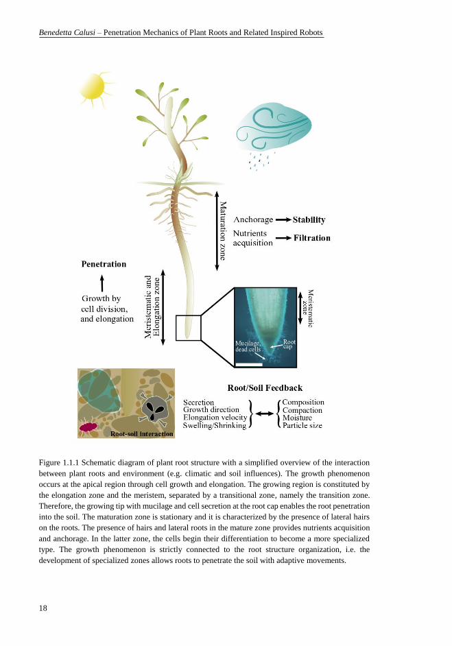
Figure 1.1.1 Schematic diagram of plant root structure with a simplified overview
of the interaction between plant roots and environment (e.g. climatic and soil
influences). The growth phenomenon occurs at the apical region through cell
growth and elongation. The growing region is constituted by the elongation zone
and the meristem, separated by a transitional zone, namely the transition zone.
Therefore, the growing tip with mucilage and cell secretion at the root cap enables
the root penetration into the soil. The maturation zone is stationary and it is
characterized by the presence of lateral hairs on the roots. The presence of hairs
and lateral roots in the mature zone provides nutrients acquisition and anchorage.
In the latter zone, the cells begin their differentiation to become a more
specialized type. The growth phenomenon is strictly connected to the root
structure organization, i.e. the development of specialized zones allows roots to
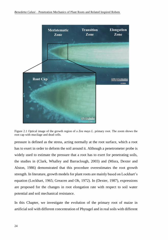
penetrate the soil with adaptive movements. ........................................................ 18 Figure 2.1 Optical image of the growth region of a Zea mays L. primary root. The
zoom shows the root cap with mucilage and dead cells. ....................................... 24 Figure 2.1.1 Flow chart of FRC (Fracture Regrowth Cycle) and the condition of
the threshold axial pressure. Each cycle starts with the initial length equal to the
growing zone length and ends when the axial stress, 𝑝 ∗, at the contact reaches
soil failure, 𝑝𝑓𝑟 ∗. Therefore, the root relaxes, the increase in root length is stored,
and a new cycle starts with the updated root length. Otherwise, the root can grow
until the growth critical pressure, 𝑝𝑐 ∗, and there is no fracture of the elastic
matrix. ................................................................................................................... 26 Figure 2.1.2 Diagram of (a) the domain for the plant root and soil, and (b) the
inclusion problem applied to the domain related to the growing region. The
growing zone of the root is a cylinder, C, and is subjected to axial and radial
pressure. The surrounding soil, M, is such that 𝑀 = 𝐶 +∪ 𝐶 − with the
cylindrical hole subjected to axial and radial pressure. ......................................... 27
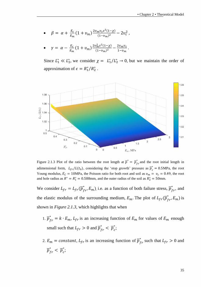
Figure 2.1.3 Plot of the ratio between the root length at 𝑝 ∗= 𝑝𝑓𝑟 ∗and the root
initial length in adimensional form, 𝐿𝑓𝑟/𝐿(𝑡0), considering the ‘stop growth’
pressure as 𝑝𝑐 ∗= 0.5MPa, the root Young modulus, 𝐸𝐶 = 10MPa, the Poisson
ratio for both root and soil as 𝜐𝑚 = 𝜐𝑐 = 0.49, the root and hole radius as 𝑅 ∗=
𝑅1 ∗= 0.588mm, and the outer radius of the soil as 𝑅2 ∗= 50mm. .................... 35 Figure 2.2.1 Comparison of the experimental data (red circles) in artificial soils
(mean values ±SD) and analytical solution (blue line) in (a) 0.15%, (b) 0.3%, (c)
0.6% Phytagel concentration. Each step of the analytical solution represents a
cycle, which ends with the fracture of the soil and begins after the relaxation of
the root. ................................................................................................................. 38 Figure 2.2.2 Comparison of the experimental data (red circles) in artificial soils
(mean values ±SD) and analytical solution (blue line) in (a) 0.9% and (b) 1.2%
Benedetta Calusi – Penetration Mechanics of Plant Roots and Related Inspired Robots
6
Phytagel concentration. Each step of the analytical solution represents a cycle,
which ends with the fracture of the soil and begins after the relaxation of the root.
.............................................................................................................................. 39 Figure 2.2.3 Comparison of the experimental data (red circles) in real soils and
analytical solution (blue lines) in (a) low, (b) medium, and (c) high compaction.
Each step of the analytical solution represents a cycle, which ends with the
fracture of the soil and begins after the relaxation of the root. ............................. 40 Figure 2.2.4 (a) In each soil medium we evaluated the variation of the root length
at the sixth day of life, by considering all the combinations of the values for the
scaling parameter γ* of the input power from the plant seed, exploited in the
numerical solution (Table 1); (b) The dotted line represents the variation in the
root length in the numerical solutions of Figure 2.2.1-Figure 2.2.3; (c) The linear
fit of γ* and different concentrations of Phytagel (R-squared: 0.97; y = a‧x, a =
5.346‧10-3 MPa‧mm3/s). ........................................................................................ 41 Figure 3.1.1 Schematic diagram of the root control mechanism to nutrient stress.
This mechanism could be similar to salt toxicity as observed in (Li et al., 2014). A
possible adaptive strategy to nutrient stress could be the enlargement of cells,
inducing a swelling of root apex. This strategy should help cells to up-take more
water and create a stronger barrier to reduce toxic nutrient concentration (Li et al.,
2014). The initial conditions are differently updated if the root activates the radial
swelling as response to nutrient stress. In such a case, the initial root length,
diameter, and cell volume are updated and stored, otherwise only the root initial
length is stored. Specifically, each cycle starts with updated initial conditions and
ends when the soil medium fractures, i.e. the axial stress, 𝑝 ∗, at the contact equals
the soil failure, 𝑝𝑓𝑟 ∗. Therefore, the root relaxes and a new cycle starts with the
updated initial conditions. Otherwise the fracture in the matrix does not occur and
the root grows until the growth critical pressure, 𝑝𝑐 ∗. ........................................ 48
Figure 3.2.1 Numerical solution of length (a) and radius (b) evolution and axial
(c) and radial (d) pressure against time. The red circles are the experimental data
(mean values ±SD) in MS4 concentration. ........................................................... 52 Figure 3.2.2 Numerical solution of length (a) and radius (b) evolution and axial
(c) and radial (d) pressure against time. The red circles are the experimental data
(mean values ±SD) in MS1 concentration. ........................................................... 53 Figure 3.2.3 Numerical solution of length (a) and radius (b) evolution and axial
(c) and radial (d) pressure against time. The red circles are the experimental data
(mean values ±SD) in MS2 concentration. ........................................................... 54 Figure 3.2.4 Numerical solution of length (a) and radius (b) evolution and axial
(c) and radial (d) pressure against time. The red circles are the experimental data
(mean values ±SD) in MS3 concentration. ........................................................... 55 Figure 4.1 Plant root structure. In the maturation zone, the cells complete their
differentiation and, providing anchorage and nutrient acquisition, lateral roots and
• List of Figures •
7
root hairs grow. Then, in the growing zone, cell division and elongation occur.
Therefore, the root elongates and penetrates the soil in the apical region. The
penetration is due to the movements localized from the root tip to the beginning
of the maturation region. ....................................................................................... 59 Figure 4.2 (a) “Vicia faba: A, radicle beginning to bend from the attached little
square of card; B, bent at a rectangle; C, bent into a circle or loop, with the tip
beginning to bend downwards through the action of geotropism.” from (Darwin
and Darwin, 1880). (b) A Borlotti Lamon bean (Phaseolus vulgaris L.) exposed to
light during growing in a 2D-confinement. The scale bar equals 2000 µm. ......... 60 Figure 4.3 Tensile tests performed on Zea mays primary roots: (a) close to and (b)
far from the tip. ..................................................................................................... 61 Figure 4.1.1 View of a nanoindentation experiment. a) A nanoindentation test.
The zoom shows the indenter tip; b) and c) a sample holder used to test
mechanical properties of root tissues near to the cap, and in outer and inner areas,
respectively; d) separation procedure of the outer wall from the inner core. ........ 63 Figure 4.1.2 Schematic of the setup used for testing along the root in water at
different distances from the tip. ............................................................................ 63 Figure 4.1.3 Plot of the mean and SD of the storage modulus at (a) the intact root
and (b) the inner tissue. ......................................................................................... 68 Figure 4.1.4 Plot of the mean and SD of the loss modulus at (a) the intact root and
(b) the inner tissue. ................................................................................................ 69 Figure 4.2.1 Overview of the contact angle measurements on the surface close to
the apical and maturation zone. ............................................................................. 73 Figure 4.2.2 Grayscale images of the wettability experiments. We analysed the
corresponding rotated zooms at a) the surface close to seed and b) the apical
region. ................................................................................................................... 73 Figure 4.3.1 A 3/4-day old Zea mays L. root, scale bar: 5mm. (a) The apical zone
is the most sensitive region of the root. Cell division and elongation occur at the
apical region and allow the root to move and grow into the soil. The cell division
is slower in the quiescent centre, then the cells mainly elongate and differentiate
in the elongation zone. The root cap has the role of protection from the
surrounding soil; (b) Fracture of the outer wall and intact inner core; (c) Twist of
the inner core; (d) Water and nutrients can move across the root through different
internal pathways: Apoplast, Transmembrane, and Symplast pathways. In this
regard, the Casparian strip is in the Apoplast pathway, limiting the water and
solute movement due to the presence of suberin (image from (Taiz and Zeiger,
1991)). ................................................................................................................... 75 Figure 4.3.2 Images of fracture due to manipulation of the root tissues of the
whole root a) and of the inner skeleton b). The tightening of the knot without
fracture of the tissue is possible only at the inner tissue level. ............................. 76
Benedetta Calusi – Penetration Mechanics of Plant Roots and Related Inspired Robots
8
Figure 4.3.3 An example of water drops sitting on root hairs (on the left) with its
schematic diagram (on the right). The surface close to the seed is covered with
dense root hairs. Thus, the hydrophobic properties could be strengthened by
surfaces textures and amplified by the presence of the root hairs. Moreover, an
air-solid state could arise from root hairs due to the air trapped below the drop. 78 Figure 4.3.4 Images showing an air-solid state arising from the presence of root
hairs on the surface close to the seed (observations on N=6 samples). ................ 79 Figure 4.3.5 Droplets with different shapes along a plant root due to the variation
of the height and distribution of hairs on the root surface. ................................... 80 Figure 5.1.1 A circular polariscope diagram. The polarizer divides the incident
light waves into vertical and horizontal components and transmit only the
components parallel to the axis of polarization of the filter. The quarter-wave
plate is like a photoelastic material having N=1/4 and its principal axis are
oriented at an angle of 45° to the axis of the polarizer. 𝛼 is the angle between the
principal stress direction, 𝜎1 and 𝜎2, at the point under consideration in the
material and the axis of polarization of the polarizer. .......................................... 86 Figure 5.2.1 Isochromatic patterns observed in a birefringent circular disk under
diametric compression. (a) ordinary isochromatic pattern; (b) ordinary
isochromatic pattern by increasing three times the applied load; (c) three times
multiplication by applying the same load as in (a). .............................................. 88 Figure 5.3.1 The plants grow in two possible types of plastic boxes. (a) The box is
open at the top and close at the bottom; (b) The box is close at the top and open to
the bottom to allow the possibility to extend the surface as the configuration (c),
by placing a box of type (a) beside a box of type (b). .......................................... 89 Figure 5.3.2 (a) The optical system for fringe multiplication technique and (b) its
schematic diagram (modified image from (Doyle and Phillips, 1989)). S – Light
Source; L – Lens; P – Polarizer; λ/4 – Quarter-wave plate; A – Analyzer. .......... 90 Figure 5.3.3 Isochromatic patterns developed by a Borlotti root (Phaseolus
vulgaris) in edible gelatine illustrating photoelastic fringe multiplication by
factors of (a) 1 and (b) 3. (c) The corresponding lateral view of the plant roots in
the photoelastic set-up after 3 days 1h from the beginning of the photoelastic
experiment. ........................................................................................................... 91 Figure 5.3.4 Development of a Borlotti root (Phaseolus vulgaris) in edible
gelatine at different growth times with the root tested by keeping the light on
during the all duration of the experiment. See Figure 5.3.3c for the lateral view of
the root at t ~ 3 days 1h. The growth time t =0 is the starting time of the
photoelastic experiment, i.e. the sample is a 3/4-day old primary root. ............... 92 Figure 5.3.5 Development of a Borlotti root (Phaseolus vulgaris) in edible
gelatine at different growth times with the root tested by keeping the light on for 3
minutes of light every 15 minutes for all the experiment duration. On the right the
• List of Figures •
9
corresponding lateral view of the plant roots in the photoelastic set-up after 3 days
15h from the beginning of the photoelastic experiment. ....................................... 93 Figure 5.3.6 Development of a Borlotti root (Phaseolus vulgaris) in edible
gelatine at different growth times with the root tested by keeping the light on for 1
minutes of light every 15 minutes for all the experiment duration. On the right the
corresponding lateral view of the plant roots in the photoelastic set-up at t ~ 3
days 18h from the beginning of the photoelastic experiment and just before the
arise of the fracture inside the gelatine. ................................................................. 93 Figure 5.4.1 The evolution of the first fringe during the FRC by applying the
growth model in Chapter 2 to the growth data (Phytagel E), by using fσ= 5.22
N/m. ....................................................................................................................... 95 Figure A.1 a) Lumped parameters model of a typical tensile testing device, where
the sample can be modeled like a spring whose characteristic shows a softening
branch; b) Global behavior of the system consisting of both the load sensor and
the sample, showing the relationship between the force (F) corresponding to the
applied displacement (xS). When the sample enters in the softening regime, F may
increase (line a)) or decrease (either line b) or c)) with xS, depending on the
magnitude of the slope of the sample characteristic, ∂F/∂(xS-xLS), compared to the
load sensor stiffness, kLS. In particular, line b) corresponds to ∂F/∂(xS-xLS)<0 and
kLS>|∂F/∂(xS-xLS)|, c) ∂F/∂(xS-xLS)<0 and kLS<|∂F/∂(xS-xLS)|. In order to evaluate
the stability of the equilibrium position of the load sensor, its dynamic behavior
can be linearized and modeled about such position through a Jacobian matrix. c)
The sign of the trace, τ, and the determinant, Δ, of the Jacobian matrix determine
the stability of the equilibrium point. .................................................................. 115

Benedetta Calusi – Penetration Mechanics of Plant Roots and Related Inspired Robots
10
• List of Tables •
11
List of Tables
Table 1 Values of parameters used in the analytical results for the growth model.
............................................................................................................................... 37 Table 2 Estimated value of the parameter 𝛾 ∗ related to the nutrient availability. In
the control concentration, i.e. without nutrient in the soil medium, the plant seed
furnishes the nutrient for the growth and is the parameter labelled as 𝛾𝐶𝑐 ∗ in the
current Section. ..................................................................................................... 51 Table 3. Storage and loss moduli (mean value ± SD) of the root cap for all
frequencies (1, 3, 10, 15, 35, 85, 200 Hz). A total of 7 indentations on 4 roots
were performed. .................................................................................................... 65 Table 4 Storage modulus measurements (mean value ± SD) along the inner core at
different distances from the tip (2, 3, 4, 5 mm) and the intact root tissue (2, 3, 4, 5,
6, 7 mm) for all frequencies (1, 3, 10, 15, 35, 85, 200 Hz). The measurements
number for each distance is reported. .................................................................... 66 Table 5 Loss modulus measurements (mean value ± SD) along the inner core at
different distances from the tip (2, 3, 4, 5 mm) and the intact root tissue (2, 3, 4, 5,
6, 7 mm) for all frequencies (1, 3, 10, 15, 35, 85, 200 Hz). The measurements
number for each distance is reported. .................................................................... 67 Table 6 Results of the Kruskal-Wallis test for the significance of the
measurements of E’ obtained at inner and intact root outer tissue levels for each
frequency at the distances of 2, 3, 4 and 5mm from the tip (df= degrees of
freedom). ............................................................................................................... 70 Table 7 Results of the Kruskal-Wallis test for the significance of the
measurements of E’ obtained at inner and intact root outer tissue levels for each
distance from the tip at all the frequencies 200, 85, 35, 15, 10, 3, 1Hz (df=
degrees of freedom). .............................................................................................. 70 Table 8 Results of the Kruskal-Wallis test for the significance of the
measurements of E’’ obtained at inner and intact root outer tissue levels for each
frequency at the distances of 2, 3, 4 and 5mm from the tip (df= degrees of
freedom). ............................................................................................................... 71 Table 9 Results of the Kruskal-Wallis test for the significance of the
measurements of E’’ obtained at inner and intact root outer tissue levels for each
distance from the tip at all the frequencies 200, 85, 35, 15, 10, 3, 1Hz (df=
degrees of freedom). .............................................................................................. 71 Table 10 Results of the one-way ANOVA test for the significance of the
measurements of the storage (E’) and loss (E’’) moduli obtained near the root cap
tip at all the frequencies 200, 85, 35, 15, 10, 3, 1Hz (Df= degrees of freedom;
Sum Sq= sum square; Mean Sq= mean square). ................................................... 72

Benedetta Calusi – Penetration Mechanics of Plant Roots and Related Inspired Robots
12

• Summary •
13
Summary
The ability of plant roots to penetrate soils is affected by several stimuli from the
surrounding medium such as mechanical stresses and chemical changes. Therefore,
roots have developed multiple responses to the several outer stimuli. Since plant
roots have to face very complex problems to grow deeply into the ground, they are
remarkable examples of problem-solving behaviour and adaptation to the outer
constraints. The adaptation strategies of a natural root are not yet completely known
and understood with exhaustive explanations. For this reason, mathematical models
and experimental techniques applied to biological phenomena can perform a key
role in translating the Nature adaptive solutions into engineering applications. The
aim of this thesis is therefore to provide further insights in understanding biological
phenomena for the development of new potential technologies inspired by the
adaptive ability of plant roots, e.g. for environmental exploration, monitoring
systems, rescue tasks, and biomedical fields. Accordingly, we proposed both
theoretical and experimental explanations to the adaptive behaviour of plant roots.
The mathematical modelling is based on a modified version of the extended (Guiot,
Pugno and Delsanto, 2006) West, Brown and Enquist universal law (West, Brown
and Enquist, 2001), considering the root growth as an inclusion problem. We
showed that the proposed equation has as a particular case a growth equation
exploiting an approach similar to Lockhart (Lockhart, 1965) taking into account the
soil impedance. We studied the influence of mechanical stresses and nutrient
availability on the root growth. Firstly, we applied the developed theoretical
framework for the strategy adopted by plant roots of a growing tip in natural soils
and of the root behaviour in response to different soil impedances with data from
both natural and artificial soils. The model predicted a different variation of the root
final length in artificial and real soils. Unexpectedly, we obtained a greater
elongation in the highest compaction for the case of artificial soils and a lower
elongation in the highest compaction for real soils. The results were in agreement

Benedetta Calusi – Penetration Mechanics of Plant Roots and Related Inspired Robots
14
with experimental data. Secondly, by coupling mechanical stress with nutrient
stimuli, we adopted an activation mechanism of the root response to the nutrient
availability in order to model the radial expansion. In particular, we proposed an
extension of the previous mathematical model by including a radial expansion
through a critical threshold. We compared the numerical solution of the analytical
model with experimental data collected in artificial soils.
In addition, we investigated the theories and hypotheses of the root ability to grow
in the apical region through nanoindentation, wettability, and photoelasticity. The
first technique provided insights for the possible role and function at both different
tissues levels and distances from the tip in the root movement and penetration
during the growth. The investigation of root tissue properties revealed that the
penetration and adaptation strategies adopted by plant roots could be enhanced by
a combination of soft and stiff tissues. The second technique aimed to highlight the
wettability of the apical zone and root hairs for the acquisition of water and
nutrients. Finally, photoelastic experiments provided a non-invasive and in situ
observation of plant roots growth and, by exploiting the fringe multiplication, we
proposed a set up for the study of plant roots growing in edible gelatine.

• Chapter 1 • Introduction
15
Chapter 1
1. Introduction
1.1. Bioinspired Engineering
In their evolution, humans have developed several methods, design and materials
to improve the quality of their life. However, such solutions could frequently have
a negative impact on the environment, e.g. the presence of pollutants in both air and
water damaging all species living on the Earth. On the contrary, Nature has
developed effective mechanisms by continuously adapting in order to withstand the
environment changes. Specifically, several examples of optimal efficiency in
design and fabrication can be found in Nature, such as bees’ honeycomb, spider’s
web, gecko adhesion and lotus’ self-cleaning, see e.g. (Bar-Cohen, 2006; Cranford
et al., 2012). Moreover, it is relevant how animals and plants evolved strategies to
adapt and maintain stability during their movements, from climbing abilities to soil
anchorage. Therefore, science and engineering are both interested in the principles
exploited by Nature (Darwin and Darwin, 1880; Dougal, 1987; Full, 2002; Goriely
and Neukirch, 2006; Baluška et al., 2009; Isnard and Silk, 2009; Roppolo et al.,
2011; Margheri et al., 2011; Crouzy, Edmaier and Perona, 2014; Tramacere et al.,
2014; Edmaier et al., 2014; Mazzolai, Beccai and Mattoli, 2014; Popova,
Tonazzini, et al., 2016). The transfer of such biological mechanisms into novel
technologies and solutions can lead to a great improvement in engineering
applications (Laschi et al., 2012; Hawkes et al., 2014; Tricinci et al., 2015; Pope et
al., 2017). In particular, the translation of Nature’s adaptive strategies into
engineering applications could provide smart solutions with tunable properties, e.g.
films with controlled surface wettability (Wang et al., 2017). In addition, the use of
a bioinspired approach could lead to the development not only of efficient devices
but also of environment-friendly technologies. The nest of birds and silk
fabrication, e.g. of spiders and silkworm, are remarkable examples of Nature’s
ability to produce sustainable, smart and effective solutions. In this regard, a recent

Benedetta Calusi – Penetration Mechanics of Plant Roots and Related Inspired Robots
16
study shows the existence of worms eating plastic that leads to a potential solution
for plastic degradation (Bombelli, Howe and Bertocchini, 2017). Furthermore,
another recent research investigates and translates the hairy structure of aquatic
plant leaves for oil/water selective separation with biodegradable and recyclable
polymers (Kavalenka et al., 2017; Zeiger et al., 2017). Therefore, Nature is the
perfect teacher for the creation of robust, efficient, and optimized ideas which
provide benefits to both the environment and the economy. The study and
translation of Nature’s adaptive strategies could have a positive effect on the
sustainability and economic development.
Recently, plant roots have inspired new principles and new technological solutions:
plant-inspired robots, called PLANTOIDs (Mazzolai, 2017), which aim at
efficiently moving into the soil by artificial roots that can grow, sense, and bend
(Sadeghi et al., 2014, 2017), by exploiting the adaptive penetration strategies of the
natural counterpart. One of the main challenges in describing the penetration of
plant roots is the active interaction between the root and the soil, i.e. the presence
of a simultaneous and mutual dependence on their evolutions and changes (Figure
1.1.1). In fact, roots adapt themselves to unexpected environment changes with
several responses, e.g. the shrinking of the diameter, the root-structure architecture,
the secretion (Barley, 1963; A. G. Bengough and Mullins, 1990; Li et al., 2014;
Popova, van Dusschoten, et al., 2016), by leading further changes in the
surrounding medium. Thus, plant roots move inside the soil by growing at the apical
zone with several and not yet completely known regulation mechanisms. One of
the first steps towards a better understanding of the root penetration is the
knowledge and definition of the key parameters to simplify the variables involved.
The penetration mechanisms and adaptation can be investigated by means of
mathematical modelling and experimental techniques. Theoretical studies have
been developed to investigate and to explain possible regulation processes that
govern the root growth, by exploiting either the control of hormone production, the
root water uptake, the root distribution on space, or the mechanical behavior at the
cellular to tissue scale, e.g. see (Chavarría-Krauser, Jäger and Schurr, 2005; Dupuy,

• Chapter 1 • Bioinspired Engineering
17
Gregory and Bengough, 2010; Dyson and Jensen, 2010; Blengino Albrieu,
Reginato and Tarzia, 2015). In this regard, experimental investigations can
estimate essential aspects which mathematical models could predict and exploit,
i.e. chemical and morphological properties and variations that may depend on the
environment changes, e.g. see (Hamza et al., 2006; Peaucelle, 2014; Colombi et
al., 2017; Dietrich et al., 2017).
For the theoretical approach, two simple models from continuum mechanics have
been proposed to characterize the mechanical and nutrient influence of the
surrounding medium on the root during its growth. In addition, the root mechanical
properties, wettability of root surface and the stress distribution developed by plant
roots inside the surrounding medium have also been investigated.
Experimental frameworks will allow further to extend the proposed mathematical
modelling by considering a more complete scenario of the root growth inside a soil
medium.
Indeed, the linkage of theoretical and experimental studies could provide not only
the means to better understand the root control mechanisms (e.g. tissue bending,
mucilage secretion, and hormones production), but also contribute in defining
which aspects should be translated with artificial smart materials in devices. For
this reason, cross-disciplinary studies are crucial to shed light on the root adaptive
capability during the penetration through the soil. On this basis, a future challenge
is to inspire an effective design based on the biological phenomenon and,
consequently, to describe the connection between natural and artificial roots.
Benedetta Calusi – Penetration Mechanics of Plant Roots and Related Inspired Robots
18
Figure 1.1.1 Schematic diagram of plant root structure with a simplified overview of the interaction
between plant roots and environment (e.g. climatic and soil influences). The growth phenomenon
occurs at the apical region through cell growth and elongation. The growing region is constituted by
the elongation zone and the meristem, separated by a transitional zone, namely the transition zone.
Therefore, the growing tip with mucilage and cell secretion at the root cap enables the root penetration
into the soil. The maturation zone is stationary and it is characterized by the presence of lateral hairs
on the roots. The presence of hairs and lateral roots in the mature zone provides nutrients acquisition
and anchorage. In the latter zone, the cells begin their differentiation to become a more specialized
type. The growth phenomenon is strictly connected to the root structure organization, i.e. the
development of specialized zones allows roots to penetrate the soil with adaptive movements.

• Chapter 1 • Outline
19
1.2. Outline
The present work focused on providing further insights in understanding Nature’s
adaptive solutions for the development of innovative technologies inspired by the
penetration mechanics of plant roots. This thesis aims at studying such strategies
through mathematical modelling and experimental methods and translating them
into potential engineering applications.
Chapter 2 and 3 are devoted to mathematical modelling developed to describe the
root growth in presence of mechanical and nutrient stimuli. In fact, the ability of
plant roots to penetrate soils is affected by different stimuli, which are exerted by
the surrounding medium. In literature, studies undertook in real soils have shown
conflicting results. We supposed that this discrepancy was mainly due to the
experiment in real soils, which are intrinsically characterized by several chemical
and physical stimuli. We then compared the two growth models with experimental
data.
In particular, in Chapter 2 we investigated and modelled the biomechanical
response of the primary root of Zea mays L., grown in artificial soils at several
levels of compactness. Unlike in heterogeneous real soils, in artificial soils the
mechanical stimulation can be distinguished from all other stimuli. We developed
a mathematical model of the dynamic evolution of plant roots, based on a modified
version of the extended universal law of West, Brown and Enquist. The theoretical
results confirm the used experimental data. Our model highlighted that root
behaviour is strongly affected by the mechanical properties of the surrounding
medium and may provide a plausible theory explaining the root behaviour during
the growth inside the surrounding soil medium. This study provides further insights
for the adaptive ability of plant roots to various soil impedance constraints.
In Chapter 3, we explored the root growth with different nutrient concentrations in
artificial soils. In fact, in presence of high concentration of chemicals plants show
thicker and shorter root apparatus. This physiological enlargement of the root

Benedetta Calusi – Penetration Mechanics of Plant Roots and Related Inspired Robots
20
transversal section becomes anomalous in presence of toxic elements. In this case,
an abnormal swelling of the root diameter and an inhibition of the root elongation
occur in the apical region. Thus, we studied the response of Zea mays roots to
different nutrient concentrations in artificial soils and proposed a hypothesis of
mechanism which can be used by plants to control nutrient changes. In this regard,
we extended the model developed in Chapter 2 by including both axial and radial
growth and we proposed that the radial expansion occurs through a critical
threshold.
The exploited experimental results showed that an excess of nutrients concentration
can result toxic for the plants, which, in fact, show a shorter root system with
abnormal enlargement in the apical region.
Our experimental and theoretical findings may improve the current knowledge of
the root response to nutrient stress. In particular, this study could describe how plant
roots may regulate both the root elongation and radial expansion due to nutrient
concentrations.
Chapters 4 and 5 are devoted to experimental activities.
In Chapter 4, we analysed the mechanical properties and surface features of Zea
mays primary roots, exploiting dynamic nanoindentation and wettability tests. We
used the indentation in the apical region and measured the contact angle close both
to the tip and the seed. The mechanical results revealed higher storage modulus
along the outer wall with respect to the central skeleton. Therefore, the outer tissue
could provide a coating to induce rigidity along the whole root and inner core could
help in case of unexpected fractures of the outer wall, e.g. for the excavation of
tunnels by burrowing animals or water flow. Moreover, the contact angle tests
showed that the apical region is characterized by low wettability and the hairy
surface close the seed seem to be a highly hydrophobic surface.
The aim of this work is to implement these features into robots inspired by natural
roots. Accordingly, a soft robot with adaptable mechanical and wettability

• Chapter 1 • Outline
21
properties for both efficient penetration and selective filtration could be useful in
several fields, e.g. soil monitoring and exploration, chemical and toxic material
spill and medical applications.
In Chapter 5, we explored the growth of Phaseolus vulgaris L. primary roots in
homogeneous birefringent media using the photoelastic technique. The growth
medium is edible gelatine. The creation of an artificial growing medium with
photoelastic properties allows to directly observe the root development and to
analyse the stresses of the growing root at the same time. Plant roots generate small
stresses at the growing tip, thus only low fringe orders can be seen. Therefore, we
showed the advantages of fringe multiplication applied to the study of plant roots
growing in edible gelatine.
In Appendix, we present an additional related study. In particular, it is devoted to
mathematical modelling of instability phenomena affecting the performance of load
sensor in MEMS-based tensile testing devices.

Benedetta Calusi – Penetration Mechanics of Plant Roots and Related Inspired Robots
22

• Chapter 2 • Mathematical Model for Axial Root Growth under Soil Confinement
23
Chapter 2
2. Mathematical Model for Axial Root Growth
under Soil Confinement
Plants do not follow a rigid predefined growing plan but adjust their strategy to
environmental conditions. Upon germination, plant architecture is driven by a
genetic post-embryonic program, which is at the basis of the plant plasticity
(Foehse and Jungk, 1983; Sánchez-Calderón, Ibarra-Cortés and Zepeda-Jazo,
2013). The study in (Bradshaw, 1965) identified two types of plant plasticity based
on morphological or physiological mechanisms. Morphological mechanisms
require high energetic costs because new functional portions are produced. On the
other hand, in the physiological mechanism, the modifications occurring in
differentiated tissue are imperceptible, the process is completely reversible and the
energetic cost is very low. The two types of plasticity are continuously expressed
during plant life since they are fundamental for their own survival (Grime and
Mackey, 2002). Root system is one of the more remarkable examples of plant
plasticity because it can sense, move and respond to the external stimuli and
transmit this information to the entire plant. The root architecture is led by the root
tip, which has the entire control of root structure in the space of a few millimetres
(Filleur et al., 2005). Root tip consists of a meristematic and elongation area,
separated by a region called the transition zone (Figure 2.1). The initial cells,
namely the cells producing new tissues during root growth, are in the meristematic
zone. Therefore, the apical region interacts with the surrounding medium and can
move continuously adapting to the outer stimuli, e.g. soil impedance. Specifically,
a growing plant root can exert an estimated maximum pressure up to 1MPa (Misra,
Dexter and Alston, 1986). For maize root, the arrest of the growth has been reported
with a penetration resistance of 0.8-2MPa (Clark, Whalley and Barraclough, 2003;
Bengough et al., 2011), and in (Popova, van Dusschoten, et al., 2016) some maize
plants did not grow beyond a penetrometer resistance of 0.25MPa. The growth
Benedetta Calusi – Penetration Mechanics of Plant Roots and Related Inspired Robots
24
Figure 2.1 Optical image of the growth region of a Zea mays L. primary root. The zoom shows the
root cap with mucilage and dead cells.
pressure is defined as the stress, acting normally at the root surface, which a root
has to exert in order to deform the soil around it. Although a penetrometer probe is
widely used to estimate the pressure that a root has to exert for penetrating soils,
the studies in (Clark, Whalley and Barraclough, 2003) and (Misra, Dexter and
Alston, 1986) demonstrated that this procedure overestimates the root growth
strength. In literature, growth models for plant roots are mainly based on Lockhart’s
equation (Lockhart, 1965; Greacen and Oh, 1972). In (Dexter, 1987), expressions
are proposed for the changes in root elongation rate with respect to soil water
potential and soil mechanical resistance.
In this Chapter, we investigate the evolution of the primary root of maize in
artificial soil with different concentration of Phytagel and in real soils with different

• Chapter 2 • Theoretical Model
25
soil compactness. Furthermore, we formulate a mathematical model for root growth
based on an elastic inclusion problem (Guiot, Pugno and Delsanto, 2006). By
exploiting a continuum mechanics approach, we consider plant root as an elastic
cylinder and soil as a homogeneous elastic fracturable matrix, in agreement with
(Guiot, Pugno and Delsanto, 2006). Since we focus on the variation of the root
elongation caused by the interactions with the surrounding environment, we
consider a single isolated root growing in an axial direction. By comparing the
theoretical results with experimental data, the goal of the present work is to
investigate how the root behaviour can be affected by the mechanical interaction
between the growing root and the surrounding soil medium.
2.1. Theoretical Model
We present a mathematical model describing the effect of mechanical stresses on
plant root growth. The model shows how the axial stress at the contact affects the
plant roots growth in the surrounding environment. When the environment is hard
to penetrate, an individual root may stop growing (Popova, van Dusschoten, et al.,
2016). Therefore, a Fracture-Regrowth Cycle, FRC, was used as in (Guiot, Pugno
and Delsanto, 2006) by including also the condition that the root stops its growth
when a threshold axial pressure is reached. If 𝑝𝑓𝑟∗
is the fracture stress of the
surrounding elastic medium and 𝑝𝑐∗ is the maximum pressure that a root can exert
to grow, two cases can occur:
(a) 𝑝𝑐∗≤ 𝑝𝑓𝑟
∗. The elastic root can grow until the axial stress 𝑝
∗
reaches the critical value and there is no fracture of the elastic
matrix; i.e. the root stops growing when 𝑝∗= 𝑝𝑐
∗. It may be the
limit case of a root growing in very strong soils.
(b) 𝑝𝑐∗> 𝑝𝑓𝑟
∗. The medium strength tolerance is reached and the root
relaxes. Therefore, the growth process starts with a new initial
length.

Benedetta Calusi – Penetration Mechanics of Plant Roots and Related Inspired Robots
26
In the present study, we focus on case (b).
Figure 2.1.1 shows a flow chart for the implementation of both the concept of FRC
and the stop growth condition.
Figure 2.1.1 Flow chart of FRC (Fracture Regrowth Cycle) and the condition of the threshold axial
pressure. Each cycle starts with the initial length equal to the growing zone length and ends when the
axial stress, 𝑝∗, at the contact reaches soil failure, 𝑝
𝑓𝑟
∗. Therefore, the root relaxes, the increase in root
length is stored, and a new cycle starts with the updated root length. Otherwise, the root can grow
until the growth critical pressure, 𝑝𝑐
∗, and there is no fracture of the elastic matrix.
2.2.1. Mechanical Problem and Interpretation
We treat both the root and the surrounding medium as a linearly elastic,
homogeneous, and isotropic material. Since the time-scale of growth is longer than

• Chapter 2 • Theoretical Model
27
the time-scale of the elastic response, this latter is hypothesized as being a quasi-
static phenomenon, thus inertial forces are negligible. We denote the plant root
domain of the growing zone 𝐶, the surrounding matrix as 𝑀, and we split 𝑀 into
two subdomains 𝐶+, 𝐶−, 𝐶+ ∪ 𝐶− = 𝑀 as in Figure 2.1.2.
Figure 2.1.2 Diagram of (a) the domain for the plant root and soil, and (b) the inclusion problem
applied to the domain related to the growing region. The growing zone of the root is a cylinder, C,
and is subjected to axial and radial pressure. The surrounding soil, M, is such that 𝑀 = 𝐶+ ∪ 𝐶− with
the cylindrical hole subjected to axial and radial pressure.
We assume that the plant root domain, 𝐶, is cylindrical, with radius1 𝑅∗, and that
the growth occurs only in the axial direction. The cylinder is closed at both ends
and subjected to the outer pressure 𝑝∗ on the bottom surface at 𝑧∗ = 𝐿∗ and 𝑝∗ in
the radial direction. The upper part of the matrix is a linear elastic isotropic thick-
walled cylinder, 𝐶+, of inner and outer radii 𝑅1∗ and 𝑅2
∗ , respectively. 𝑝∗ is the
1 The superscript “*” denotes dimensional variables.

Benedetta Calusi – Penetration Mechanics of Plant Roots and Related Inspired Robots
28
pressure applied at 𝑅1∗. We then consider a linear elastic isotropic cylinder, 𝐶−, of
radius 𝑅2∗. We suppose that the cylinder 𝐶− is closed at bottom end (at 𝑧∗ = 𝐿2
∗ )
and the top end is subjected to axial pressure 𝑝∗ over a circle of radius 𝑅1
∗. In order
to meet the experimental conditions, we require that there is no displacement over
the whole outer surface of 𝑀. We assume that the displacement vector is
𝒖∗(𝑟∗, 𝜃∗, 𝑧∗) = (𝑢𝑟∗∗ , 𝑢𝜃∗
∗ , 𝑢𝑧∗∗ ) = (𝑢𝑟∗
∗ (𝑟∗), 0, 𝑢𝑧∗(𝑧∗)), (1)
thus, for the cylinders 𝐶±, 𝐶 we have
∇∗ × 𝒖∗ = 0. (2)
First, we compute stresses and displacements in the elastic matrix, 𝑀 , with a
cylindrical hole, and then in the elastic cylinder, 𝐶.
In the case of elastic matrix, the equation (2) has the following solution2
{
𝑢𝑟∗
∗ +(𝑟∗) =
𝐶1+𝑟∗
2+𝐶2+
𝑟∗ 𝑖𝑛 𝐶+,
𝑢𝑧∗∗ +(𝑧∗) = 𝐶3
+𝑧∗ + 𝐶4+ 𝑖𝑛 𝐶+,
𝑢𝑟∗∗ −(𝑟∗) =
𝐶1−𝑟∗
2 𝑖𝑛 𝐶−,
𝑢𝑧∗∗ −(𝑧∗) = 𝐶3
−𝑧∗ + 𝐶4− 𝑖𝑛 𝐶−,
where 𝑢∗+, 𝑢∗− are the displacements of the upper and lower part of the matrix,
respectively. Thus, we look for values of the constants such that the following
boundary conditions
{
𝜎𝑟∗𝑟∗∗ + = −𝑝∗ 𝑟∗ = 𝑅1
∗, 𝑧∗ ∈ (0, 𝐿1∗ ),
𝑢𝑟∗∗ +(𝑅2
∗) = 0 𝑧∗ ∈ (0, 𝐿1∗ ),
𝑢𝑟∗∗ +(𝑅2
∗) = 0 𝑧∗ ∈ (𝐿1∗ , 𝐿2
∗ ),
𝑢𝑧∗∗−(𝐿2
∗ ) = 0 𝑟∗ ∈ (0, 𝑅2∗),
𝑢𝑧∗∗ +(𝐿1
∗ ) = 𝑢𝑧∗∗ −(𝐿1
∗ ) 𝑟∗ ∈ (𝑅1∗, 𝑅2
∗),
𝑢𝑧∗∗ +(0) = 0 𝑟∗ ∈ (𝑅1
∗, 𝑅2∗),
2 All the derivatives with respect to 𝜃∗ vanish and there is no dependence of the angle 𝜃∗.

• Chapter 2 • Theoretical Model
29
and the following equilibrium
𝜋𝜎𝑧∗𝑧∗∗ + (𝑅2
∗2 − 𝑅1∗2) − 𝜋𝑝
∗𝑅1∗2 = 𝜋𝜎𝑧∗𝑧∗
∗ − 𝑅2∗2 𝑧∗ = 𝐿∗, 𝑟∗ ∈ (0, 𝑅∗),
are satisfied. By neglecting the terms of higher order then 휀2, we obtain
𝐶1+ =
−2𝑝∗𝜖2
𝐸𝑚(1 + 𝜈𝑚),
𝐶2+ =
𝑅1∗2(1 + 𝜈𝑚)𝐸𝑚
{�̅�∗𝜖2𝜈𝑚(1 − 𝜒)
1 − 𝜈+ 𝑝∗ [1 +
𝜖2
1 − 2𝜈𝑚(−1 +
2𝜈𝑚2 (1 − 𝜒)1 − 2𝜈𝑚
)]} ,
𝐶3− =
𝜖2𝜒𝐸𝑚(1 − 𝜈𝑚)
(�̅�∗ + 𝑝∗2𝜈𝑚
1 − 2𝜈𝑚),
𝐶1− = 0, 𝐶4− = 0,
where 𝜒 = 𝐿1∗ /𝐿2
∗ , 𝜖 = 𝑅1∗/𝑅2
∗, 𝜐𝑚, 𝐸𝑚 are the Poisson ratio and Young modulus of
the elastic medium, respectively.
In a similar way, in the case of the elastic cylinder, the solution of the equation (2)
is given by 𝑢𝑟∗∗ (𝑟∗ ) =
𝐶1𝑟∗
2 and 𝑢𝑧∗
∗ (𝑧∗) = 𝐶3𝑧∗ with (𝑟∗, 𝑧∗) ∈ 𝐶 . By imposing
the following boundary conditions
{
𝜎𝑟∗𝑟∗∗ = −𝑝∗ 𝑟∗ = 𝑅∗, 𝑧∗ ∈ (0, 𝐿∗),
𝜎𝑧∗𝑧∗∗ = −𝑝
∗ 𝑧∗ = 𝐿∗, 𝑟∗ ∈ (0, 𝑅∗),
𝑢∗(0) = 0,
the solution, in the case of the elastic cylinder, is given by 𝐶1 =
−𝑝∗(1−𝜈𝑐)+𝜈𝑐𝑝
∗
𝐸𝑐, 𝐶3 =
2𝜈𝑐𝑝∗−𝑝
∗
𝐸𝑐, where 𝜐𝑐 , 𝐸𝑐 correspond to the elastic cylinder
coefficients, respectively. In order to have the contact at the interface between the
matrix and the elastic cylinder, we require the following compatibility equation
{𝑅∗ + 𝑢𝑟∗
∗ (𝑅∗) = 𝑅1∗ + 𝑢𝑟∗
∗ +(𝑅1
∗),
𝐿∗ + 𝑢𝑧∗∗ (𝐿∗) = 𝐿1
∗ + 𝑢𝑧∗∗ +(𝐿1
∗ ),
the radius and length of the deformed elastic root are equal to the radius and length
of the deformed matrix, respectively. By exploiting the compatibility conditions at

Benedetta Calusi – Penetration Mechanics of Plant Roots and Related Inspired Robots
30
the contact and after some algebra, we obtain the expressions for radial, 𝑝∗, and
axial pressure, 𝑝∗, in a dimensional form
�̅�∗ = 𝐸𝑐(1 − 𝜈𝑐)(𝑅
∗ + 𝑅1∗𝐴2)(𝐿
∗ − 𝐿1∗ ) + 2𝜈𝑐(𝐿
∗ − 𝐿1∗𝐴1)(𝑅
∗ − 𝑅1∗)
(1 − 𝜐𝑐)(𝑅∗ + 𝑅1
∗𝐴2)(𝐿∗ + 𝐿1
∗𝐵1) − 2𝜈𝑐2(𝐿∗ − 𝐿1
∗𝐴1)(𝑅∗ − 𝑅1
∗𝐴1) , (3.1)
𝑝∗ = 𝐸𝑐𝜈𝑐(𝑅
∗ − 𝑅1∗𝐴1)(𝐿
∗ − 𝐿1∗ ) + (𝐿∗ − 𝐿1
∗𝐵1)(𝑅∗ − 𝑅1
∗)
(1 − 𝜐𝑐)(𝑅∗ + 𝑅1
∗𝐴2)(𝐿∗ + 𝐿1
∗𝐵1) − 2𝜈𝑐2(𝐿∗ − 𝐿1
∗𝐴1)(𝑅∗ − 𝑅1
∗𝐴1) , (3.2)
where
• 𝐴1 = 𝜖2 𝐸𝑐
𝐸𝑚𝜐𝑚
(1−𝜒)(1+𝜐𝑚)
𝜈𝑐(1−𝜐𝑚),
• A2 =𝐸𝑐
𝐸𝑚
(1+𝜐𝑚)
(1−𝜐𝑐)[1 − 𝜖2 +
𝜀2
1−2𝜐𝑚 (2𝜐𝑚
2 (1−𝜒)
1−𝜐𝑚− 1)] ,
• B1 = 𝜖2 𝐸𝑐
𝐸𝑚(1 − 𝜒)(1 + 𝜐𝑚)
• 𝜖 =𝑅1∗
𝑅2∗ , 𝜒 =
𝐿1∗
𝐿2∗ .
2.2.2. Axial Growth Equations
By exploiting a similar approach to Lockhart (Lockhart, 1965) and by taking into
account the soil impedance as in (Greacen and Oh, 1972; Dexter, 1987; Bengough,
Croser and Pritchard, 1997; Bengough et al., 2006), we can describe the growth
process with the following model3
1
𝑉∗𝑑𝑉∗
𝑑𝑡∗= 𝛷∗ (𝑝𝑐
∗− 𝑝
∗)+, (4)
where 𝛷∗, [𝛷∗] = (MPa ∙ s)−1, is related to the extensibility of wall of a plant cell
and 𝑝𝑐∗ is the threshold value introduced at the beginning of Section 2.1. The model
(4) captures the most commonly accepted phenomenon related to the influence of
3 (𝑓(𝑥))+ = max (𝑓(𝑥),0) = {𝑓(𝑥), 𝑓(𝑥) > 00, 𝑜𝑡ℎ𝑒𝑟𝑤𝑖𝑠𝑒
is the positive part of 𝑓(𝑥).
• Chapter 2 • Theoretical Model
31
soil physical properties on root growth, i.e. roots grow slower in denser soils.
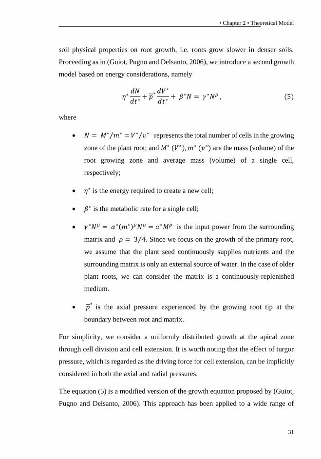
Proceeding as in (Guiot, Pugno and Delsanto, 2006), we introduce a second growth
model based on energy considerations, namely
𝜂∗𝑑𝑁
𝑑𝑡∗+ 𝑝
∗ 𝑑𝑉∗
𝑑𝑡∗+ 𝛽∗𝑁 = 𝛾∗𝑁𝜌 , (5)
where
• 𝑁 = 𝑀∗ 𝑚∗ =⁄ 𝑉∗ 𝑣∗⁄ represents the total number of cells in the growing
zone of the plant root; and 𝑀∗ (𝑉∗),𝑚∗ (𝑣∗) are the mass (volume) of the
root growing zone and average mass (volume) of a single cell,
respectively;
• 𝜂∗ is the energy required to create a new cell;
• 𝛽∗ is the metabolic rate for a single cell;
• 𝛾∗𝑁𝜌 = 𝛼∗(𝑚∗)𝜌𝑁𝜌 = 𝛼∗𝑀𝜌 is the input power from the surrounding
matrix and 𝜌 = 3 4⁄ . Since we focus on the growth of the primary root,
we assume that the plant seed continuously supplies nutrients and the
surrounding matrix is only an external source of water. In the case of older
plant roots, we can consider the matrix is a continuously-replenished
medium.
• 𝑝∗
is the axial pressure experienced by the growing root tip at the
boundary between root and matrix.
For simplicity, we consider a uniformly distributed growth at the apical zone
through cell division and cell extension. It is worth noting that the effect of turgor
pressure, which is regarded as the driving force for cell extension, can be implicitly
considered in both the axial and radial pressures.
The equation (5) is a modified version of the growth equation proposed by (Guiot,
Pugno and Delsanto, 2006). This approach has been applied to a wide range of

Benedetta Calusi – Penetration Mechanics of Plant Roots and Related Inspired Robots
32
biological phenomena (West, Brown and Enquist, 1997; Bettencourt et al., 2007).
For example, the authors of (Guiot, Pugno and Delsanto, 2006) developed a model
for tumour invasion, considering the effect of interfacial pressure as an extension
of the West, Brown and Enquist law (West, Brown and Enquist, 2001). The root
elongation rate is sensitive to variations in axial pressure (Bengough and
Mackenzie, 1994; Bengough, 2012), but insensitive to radial pressure (Kolb,
Hartmann and Genet, 2012). This aspect explains the presence of the mechanical
term in equations (4) and (5) due to the axial pressure. We will further assume that
root is cylindrical (as in Figure 2.1.2) and grows only in length. Therefore, an
increase in length is related to an increase in volume and in the number of cells
through
𝑑𝐿∗
𝑑𝑡∗=
1
𝜋𝑅∗2 𝑑𝑉∗
𝑑𝑡∗=
𝑣0∗
𝜋𝑅∗2 𝑑𝑁
𝑑𝑡∗, (6)
where 𝑣0∗ is the single cell volume that we consider constant. Note that if 𝜌 = 1 and
if 𝑝∗ is small, with proper values of 𝑣0
∗, 𝜂∗, 𝛾∗, 𝛽∗ we can recover the equation (4)
from the equation (5).
2.2.3. Adimensionalization
We scale the variables by writing
𝐿∗ = 𝐿0∗ 𝐿, 𝑡∗ = 𝑡𝑟𝑒𝑓
∗ 𝑡,
where 𝐿0∗ represents the length of the growing region from the tip to the end of the
elongation zone and 𝑡𝑟𝑒𝑓∗ is the duration of the experiment. We assume 𝐿0
∗ = 3mm
and 𝑡𝑟𝑒𝑓∗ = 3days.
We notice that 𝐿1∗ represents the initial length of the elastic cylinder in each cycle
and we assume zero pressure at both ends of the cycle. Therefore, we can write
𝐿1∗ = 𝐿0
∗ 𝐿(𝑡0), where the adimensional length 𝐿(𝑡0) is “updated” at the beginning
of each cycle.

• Chapter 2 • Theoretical Model
33
Assuming the axial growth, i.e. 𝑅∗ = 𝑅1∗, we can rewrite equations (3.1) and (3.2)
as
{
𝑝∗= Θ1
∗𝐿 − Θ2𝐿 + Θ3
,
𝑝∗ = Θ4∗𝐿 − Θ2𝐿 + Θ3
,
where
• Θ1∗ = 𝐸𝑐
𝛼
𝛽,
• Θ2 = 𝐿(𝑡0) is the root length at the beginning of the FRC;
• Θ3 =𝛾
𝛽𝜖2
𝐸𝑐
𝐸𝑚 𝐿(𝑡0)(1 − 𝜒)(1 + 𝜐𝑚),
• Θ4∗ =
𝐸𝑐
𝛽[𝜐𝑐 − 𝜖
2 𝐸𝑐
𝐸𝑚 (1 − 𝜒)
𝜐𝑚(1+𝜐𝑚)
(1−𝜐𝑚)],
• 𝛼 = 1 − 𝜐𝑐 + 𝐸𝑐
𝐸𝑚(1 + 𝜐𝑚) [1 − 𝜖
2 +𝜀2
1−2𝜐𝑚 (2𝜐𝑚
2 (1−𝜒)
1−𝜐𝑚− 1)],
• 𝛽 = 𝛼 + 𝐸𝑐
𝐸𝑚(1 + 𝜐𝑚)
2𝜐𝑚𝜐𝑐𝜀2(1−𝜒)
(1−𝜐𝑚)2 − 2𝜐𝑐
2 ,
• 𝛾 = 𝛼 − 𝐸𝑐
𝐸𝑚(1 + 𝜐𝑚)
2𝜐𝑚2 𝜀2(1−𝜒)
(1−𝜐𝑚)2 −
2𝜐𝑚𝜐𝑐
1−𝜐𝑚 ,
and [Θ1∗] = [Θ4
∗ ] = MPa and [Θ2] = [Θ3] = 1.
By considering the stop of the root growth when 𝑝∗ reaches the critical value 𝑝𝑐
∗,
from the equation (5) the following relation
𝛽∗ = 𝛾∗
(
Θ2 +Θ3
𝑝𝑐∗
Θ1∗
1 − 𝑝𝑐∗
Θ1∗)
𝜌−1
,

Benedetta Calusi – Penetration Mechanics of Plant Roots and Related Inspired Robots
34
holds and we introduce the scaling parameter Θ1∗ for the adimesionalization of the
axial pressure, 𝑝∗, as an upper bound for 𝑝𝑐
∗.
2.2.4. Stress Effects on Root Penetration
This Section focuses on how the axial stress at the contact affects the biomechanical
properties of plant roots penetration depending on the surrounding matrix. Since
the change in length is slow, every moment of the growth process can be
represented as a static state and we can interpret the mechanical process of root
growth as an inclusion model. The inclusion model analyses in detail the
mechanical expansion of an elastic cylinder in a cylindrical hole of an elastic
fracturable medium. In particular, we study the sensitivity of the root length to the
variation in the fracture stress, 𝑝𝑓𝑟∗
, and the Young modulus, 𝐸𝑚 , of the
surrounding matrix. Therefore, we analyse the variation in the root length,
𝐿𝑓𝑟∗ , when the axial contact pressure is equal to 𝑝𝑓𝑟
∗.
From the inclusion problem, we can obtain the expression of root length in the
dimensionless form (see Subsection 2.2.3) at 𝑝∗= 𝑝𝑓𝑟
∗
𝐿𝑓𝑟 = 𝐿(𝑡0) + Θ3
𝑝𝑓𝑟
∗
Θ1∗
1 − 𝑝𝑓𝑟∗
Θ1∗
, ∀ 𝑝𝑓𝑟∗< Θ1
∗ , (7)
where
• 𝐿(𝑡0) is the root length at the beginning of FRC;
• Θ1∗ = 𝐸𝑐
𝛼
𝛽,
• Θ3 =𝛾
𝛽𝜖2
𝐸𝑐
𝐸𝑚 𝐿(𝑡0)(1 − 𝜒)(1 + 𝜐𝑚),
• 𝛼 = 1 − 𝜐𝑐 + 𝐸𝑐
𝐸𝑚(1 + 𝜐𝑚) [1 − 𝜖
2 +𝜀2
1−2𝜐𝑚 (2𝜐𝑚
2 (1−𝜒)
1−𝜐𝑚− 1)],
• Chapter 2 • Theoretical Model
35
• 𝛽 = 𝛼 + 𝐸𝑐
𝐸𝑚(1 + 𝜐𝑚)
2𝜐𝑚𝜐𝑐𝜀2(1−𝜒)
(1−𝜐𝑚)2 − 2𝜐𝑐
2 ,
• 𝛾 = 𝛼 − 𝐸𝑐
𝐸𝑚(1 + 𝜐𝑚)
2𝜐𝑚2 𝜀2(1−𝜒)
(1−𝜐𝑚)2 −
2𝜐𝑚𝜐𝑐
1−𝜐𝑚 .
Since 𝐿1∗ ≪ 𝐿2
∗ , we consider 𝜒 = 𝐿1∗ 𝐿2
∗⁄ → 0, but we maintain the order of
approximation of 𝜖 = 𝑅1∗ 𝑅2
∗⁄ .
Figure 2.1.3 Plot of the ratio between the root length at 𝑝∗= 𝑝
𝑓𝑟
∗and the root initial length in
adimensional form, 𝐿𝑓𝑟/𝐿(𝑡0), considering the ‘stop growth’ pressure as 𝑝𝑐
∗= 0.5MPa, the root
Young modulus, 𝐸𝐶 = 10MPa, the Poisson ratio for both root and soil as 𝜐𝑚 = 𝜐𝑐 = 0.49, the root
and hole radius as 𝑅∗ = 𝑅1∗ = 0.588mm, and the outer radius of the soil as 𝑅2
∗ = 50mm.
We consider 𝐿𝑓𝑟 = 𝐿𝑓𝑟(𝑝𝑓𝑟∗, 𝐸𝑚), i.e. as a function of both failure stress, 𝑝𝑓𝑟
∗, and
the elastic modulus of the surrounding medium, 𝐸𝑚. The plot of 𝐿𝑓𝑟(𝑝𝑓𝑟∗, 𝐸𝑚) is
shown in Figure 2.1.3, which highlights that when
1. 𝑝𝑓𝑟∗= 𝑘 ∙ 𝐸𝑚, 𝐿𝑓𝑟 is an increasing function of 𝐸𝑚 for values of 𝐸𝑚 enough
small such that 𝐿𝑓𝑟 > 0 and 𝑝𝑓𝑟∗< 𝑝𝑐
∗;
2. 𝐸𝑚 = 𝑐𝑜𝑛𝑠𝑡𝑎𝑛𝑡, 𝐿𝑓𝑟 is an increasing function of 𝑝𝑓𝑟∗
such that 𝐿𝑓𝑟 > 0 and
𝑝𝑓𝑟∗< 𝑝𝑐
∗;
Benedetta Calusi – Penetration Mechanics of Plant Roots and Related Inspired Robots
36
3. 𝑝𝑓𝑟∗= 𝑐𝑜𝑛𝑠𝑡𝑎𝑛𝑡 < 𝑝𝑐
∗, 𝐿𝑓𝑟 is a decreasing function of 𝐸𝑚 such that 𝐿𝑓𝑟 > 0.
The above analysis highlights the importance of considering the concept of failure
stress at a small value for Young’s modulus of the elastic matrix.
In order to determine the growth, we employ the model given by the equation (5)
to the experiments in artificial soils (the experimental work related to this Chapter
has been performed by IIT). In addition, we compare our theoretical results with
data from experiments in different real soil compactions (for more details see
(Popova, van Dusschoten, et al., 2016)).
2.2. Theoretical Results
In this analysis, the surrounding medium is assumed to be an infinite body with
respect to the plant root, so that 𝑅∗, 𝑅1∗ ≪ 𝑅2
∗ and 𝐿∗, 𝐿1∗ ≪ 𝐿2
∗ . Therefore, to obtain
the numerical solutions, we set 𝜒 = 𝐿1∗ 𝐿2
∗⁄ = 0, and we assume 𝑅2∗ = 50mm for
both artificial and real soils. We then assume that the growth critical pressure 𝑝𝑐∗=
0.5 MPa (for the value range of 𝑝𝑐∗ see, e.g., (Misra, Dexter and Alston, 1986;
Clark, Whalley and Barraclough, 2003; Bengough et al., 2011; Popova, van
Dusschoten, et al., 2016)), and the root Young modulus 𝐸𝑐 = 10MPa (Forterre,
2013). We assume that 𝑅1∗ = 𝑅∗ are equal to the values of the root apex radius at
the third day of life (the related experimental work has been performed by IIT) for
artificial soil, and 𝑅1∗ = 𝑅∗ = 0.6 mm for real soils. Both Poisson’s ratios are
𝜈𝑚,𝑐 = 0.49 for Phytagel and 𝜈𝑐 = 0.49, 𝜈𝑚 = 0.45 for soils (Bowles, 1997;
Normand et al., 2000; Das, 2014). The values used for 𝛾∗, 𝐸𝑚, 𝑝𝑓𝑟∗
are reported in
Table 1 (𝐸𝑚, 𝑝𝑓𝑟∗
are obtained by means of compression tests). In order to estimate
only the variation of 𝛾∗ with respect the different soil media, a constant value for
the parameter 𝜂∗, 𝜂∗ = 35 MPa · mm3, has been chosen. Figure 2.2.1- Figure
2.2.3 show the evolution of the root length with time for artificial and real soils,
respectively.

• Chapter 2 • Theoretical Results
37
The value of the scaling parameter 𝛾∗ of the energy released from the seed
increases in the medium hardness for both artificial and real soils. By using artificial
growth media, roots, which were grown in harder soils, were longer than the roots
grown in softer soils, while in real soils this was not the case. Using 0.6% Phytagel
(Group C) we obtain a lower final length in both the numerical (Figure 2.2.4b) and
experimental results (the related experimental work has been performed by IIT). In
order to assess the influence of 𝛾∗ on the variation of the final root length, we carry
out the theoretical predictions in both artificial and real soil using all the
combinations of the value for 𝛾∗ listed in Table 1. The results by means of equation
(5) are given in Figure 2.2.4.
Phytagel is a hard and brittle homogeneous gel (Schiavi, Cuccaro and Troia, 2016)
and, because of its homogeneity, we can assume that the increase in Young
modulus leads to an increase in the fracture stress (see Subsection 2.2.4). In
addition, Figure 2.2.4c shows that 𝛾∗ increases linearly with respect to the Phytagel
concentration. Therefore, in the presence of artificial soils the increase in energy
availability and the soil mechanical properties may enhance root penetration.
Table 1 Values of parameters used in the analytical results for the growth model.
𝑬𝒎 (MPa) 𝒑𝒇𝒓
∗± 𝐒𝐃 (MPa) 𝜸∗(MPa·mm3/s)
Phytagel
Artificial soil
Group A (0.15%
Phyt. conc.)
1.02·10−2 0.0025±7.278·10-4 7.53·10-4
Group B (0.3%
Phyt. conc.)
1.82·10−2 0.0053±0.0012 1.94·10-3
Group C (0.6%
Phyt. conc.)
4.23·10−2 0.0089±0.0016 2.56·10-3
Group D (0.9%
Phyt. conc.)
7.43·10−2 0.0140±0.0018 4.76·10-3
Group E (1.2%
Phyt. conc.)
8.09·10−2 0.0141±0.0017 6.7·10-3
Low compaction 2 0.02 1.2·10-2
Real soil Medium
compaction
25 0.04 2.19·10-2
High compaction 50 0.25 0.1021

Benedetta Calusi – Penetration Mechanics of Plant Roots and Related Inspired Robots
38
Figure 2.2.1 Comparison of the experimental data (red circles) in artificial soils (mean values ±SD)
and analytical solution (blue line) in (a) 0.15%, (b) 0.3%, (c) 0.6% Phytagel concentration. Each step
of the analytical solution represents a cycle, which ends with the fracture of the soil and begins after
the relaxation of the root.
(a)
(b)
(c)

• Chapter 2 • Theoretical Results
39
Figure 2.2.2 Comparison of the experimental data (red circles) in artificial soils (mean values ±SD)
and analytical solution (blue line) in (a) 0.9% and (b) 1.2% Phytagel concentration. Each step of the
analytical solution represents a cycle, which ends with the fracture of the soil and begins after the
relaxation of the root.
(a)
(b)

Benedetta Calusi – Penetration Mechanics of Plant Roots and Related Inspired Robots
40
Figure 2.2.3 Comparison of the experimental data (red circles) in real soils and analytical solution
(blue lines) in (a) low, (b) medium, and (c) high compaction. Each step of the analytical solution
represents a cycle, which ends with the fracture of the soil and begins after the relaxation of the root.
(a)
(b)
(c)

• Chapter 2 • Theoretical Results
41
Figure 2.2.4 (a) In each soil medium we evaluated the variation of the root length at the sixth day of
life, by considering all the combinations of the values for the scaling parameter γ* of the input power
from the plant seed, exploited in the numerical solution (Table 1); (b) The dotted line represents the
variation in the root length in the numerical solutions of Figure 2.2.1-Figure 2.2.3; (c) The linear fit
of γ* and different concentrations of Phytagel (R-squared: 0.97; y = a‧x, a = 5.346‧10-3 MPa‧mm3/s).
(a)
(b)
(c)
Benedetta Calusi – Penetration Mechanics of Plant Roots and Related Inspired Robots
42
2.3. Interpretation and Discussion
The first week of plant life is a fundamental period to establish a strong anchorage
and develop a complete radical apparatus. The primary root thus represents an
interesting model to study the soil impedance response (Goodman and Ennos,
1999). By using real soils, conflicting results on the increase or decrease in root
length by varying the soil compaction and root species have been found (Barley,
1963; Taylor and Ratliff, 1969; Wilson, Robards and Goss, 1977; Wilson and
Robards, 1978; Atwell, 1989; A. Bengough and Mullins, 1990; Pietola and
Smucker, 1998; Alessa and Earnhart, 2000). Decodifying a univocal cause–effect
behaviour between root growth and soil hardness is difficult. In fact, previous
studies have been carried out in real soil, which is intrinsically characterized by
several physical and chemical complex interactions (soil aerations, water, oxygen
availability, etc.).
Alternative protocols to the use of real soil have been proposed, such as wax layers
or vertical oriented agar plates (Okada and Shimura, 1990; Materechera, Dexter
and Alston, 1991; Clark et al., 1996). One of the most common approaches is to
use transparent gelling agents such as agar and agarose, commonly used to prepare
growth media for botanical and bacterial applications. For example, (Zacarias and
Reid, 1992; Volkmar, 1994; Clark et al., 1999) all used the agar gels to study
mechanical impedance in roots because agar gel impedes the root system and
visualizes it at the same time. In accordance with these studies, we analyse the
growth kinetics of Zea mays L. primary root exploiting artificial soils (Phytagel)
with different levels of concentrations. Accordingly, we investigated the first
interaction of plant root with the soil, preventing the interference of any other
physical and chemical stimulus.
Unexpectedly, the experimental results showed that the primary roots grown in
higher concentrations of Phytagel (i.e. higher levels of compactness in the soil)
have greater elongation. In order to ascertain the plausibility of these findings in
comparison with experiments in real soils, we developed a theoretical model for

• Chapter 2 • Interpretation and Discussion
43
the mechanical process of root growth with the root-soil mechanical interaction.
Our mathematical model combines plant roots growth and the mechanical contact
with the soil through the modified version of the extended WBE universal law and
the inclusion problem.
From the theoretical results, we found that an increase in the scaling parameter 𝛾∗
(Table1) could reveal an increase in the demand of plant nutrients when the soil
medium is more compact. Since the experiments were carried out in the absence of
nutrients in the soil, the nutrient demand was addressed to the reserves stored in the
seed (primary roots) and the surrounding soil medium supplies continuously only
water. Thus, our study may reveal a relation between nutrients from the seed and
soil medium compactness. Since the mechanical impedance of the artificial soils is
weaker than real soils in terms of inducing a change in root growth, the increase in
the released energy can provide a more effective penetration in Phytagel (Figure
2.2.4). In fact, the inclusion problem could explain how, at the contact fracture
pressure, the ability of plant roots to grow changes and is influenced by the
mechanical properties of the surrounding environment.
The Young modulus of plant tissues takes typically a value of around 10 MPa
(Forterre, 2013). We assume that 𝐸𝑐 is constant so it does not change along the root
axis (i.e. with age) and the surrounding soil. In addition, we notice that 𝐿𝑓𝑟 ∗ is a
decreasing function of 𝐸𝑐 , i.e. considering a fixed medium the increase in root
stiffness seems to have a negative influence on the plant roots expansion as
remarked in (Wei and Lintilhac, 2007). Indeed, the authors of (Wei and Lintilhac,
2007) investigated aspect of turgor-driven plant cell growth with a model derived
from the Eulerian concept of instability and showed that increasing elastic modulus
of plant cell has a negative effect on wall expansion.
In conclusion, we analyse the growth kinetic of the primary root (Z. mays) in
artificial soils. In particular, we develop an ad-hoc setup and a theoretical
framework to understand the contribution played by mechanical stimuli in the root
growth. Our theoretical and experimental studies may be a further investigation to
explain how plant roots could control the growth in response to the contact with the

Benedetta Calusi – Penetration Mechanics of Plant Roots and Related Inspired Robots
44
surrounding medium and help to improve the current knowledge on the behavioural
strategies of plant roots. The mathematical model is based on continuum mechanics
and is a general formulation for the prediction of plant roots growth in soil media.
The unexpected experimental results highlight the active response of plant roots to
the changes in the surrounding medium as simulated by the theoretical model.
• Chapter 3 • Extension of the Mathematical Model including Root Radial Growth and Nutrient
Influence
45
Chapter 3
3. Extension of the Mathematical Model including
Root Radial Growth and Nutrient Influence
Plant roots have developed different defence responses to outer stimuli caused by
the surrounding soil, e.g. increase or decrease in the elongation, swelling or
shrinking of the diameter and root-structure tortuosity (Barley, 1963; A. Bengough
and Mullins, 1990; Li et al., 2014; Popova, van Dusschoten, et al., 2016). Since the
apical zone tissues are the most sensitive to the environment changes, the apex is
the first zone of the root responding to external stimuli. For this reason, several
investigations to understand how plant roots can modulate and control the effects
of external chemical and physical (mainly mechanical) stimuli on their growth can
be found, e.g. see (Wilson, Robards and Goss, 1977; Atwell, 1989; Baluska et al.,
1993; Baluska, Parker and Barlow, 1993; Baluška, Parker and Barlow, 1993;
Baluška, Busti, et al., 2001; Baluška, Jasik, et al., 2001).
In particular, many studies illustrated the evolution of root system in nutrient-rich
patches (Drew and Saker, 1978; Crick and Grime, 1987; Jackson and Caldwell,
1989, 1996; Gross, Peters and Pregitzer, 1993) analysing phenotypical reactions
(branching, root elongation, lateral root emergence, root hairs proliferation, etc.).
Since the majority of these studies were conducted in real soils (Kirby and
Bengough, 2002; Pierret et al., 2007), characterized by high heterogeneity, these
findings have to be considered as a result of several physical and chemical stimuli.
In fact, in order to properly investigate each phenomenon and carry out a rigorous
cause-effect analysis, plants should be studied in environments that allow to
distinguish each single stimulus. In order to discriminate indiscernible parameters
in a real environment (Tian and Doerner, 2013) and ascertain the response of plant
root to different nutrient concentrations, we used data of plants grown in artificial
soils in the absence of other physical or chemical stimuli.

Benedetta Calusi – Penetration Mechanics of Plant Roots and Related Inspired Robots
46
A recent research (Li et al., 2014) explains that roots exploit an adaptive strategy
to defend themselves by salt toxicity, increasing the number of stele tissue cell
layers. Such a strategy causes an evident swelling of root apex that should help cells
to up-take more water and create a stronger barrier to reduce Na+ concentration.
Furthermore, other studies show similar root apex swellings, e.g. after depletion of
giberellic acid or ethylene and high calcium exposures (Baluska et al., 1993;
Baluška, Parker and Barlow, 1993; Baluska, Hauskrecht and Barlow, 1996). In
addition, investigations on the depolymerization of F-actin with latrunculin B
reveal also in very similar maize root apex swellings and inhibition of the root cell
elongation (Baluška, Jasik, et al., 2001). The root swelling and the reduction of
primary root length were observed in maize and cotton (Kurth et al., 1986; Zidan,
Azaizeh and Neumann, 1990) and in several crop plants grown in media with high
concentration of NaCl. Aluminium is considered a source of toxicity for plants as
well, inducing structure deformation (Pietola and Smucker, 1998; Zhu, Ahn and
Matsumoto, 2003; Kynast, 2012) and swelling phenomenon (Bennet, Breen and
Fey, 1985a, 1985b; Budíková, 1999). One of the potential explanations of the
observed phenomenon could be an adaptation strategy of plant roots. In fact, plants
can be regarded as sensory and communicative organisms with active problem-
solving behaviour (Baluška et al., 2009). Although the molecular and cellular
responses are still not known, we believe that such studies will provide insights in
understanding the control and modulation of root development with several
morphological adaptations.
In this Chapter we exploited the experiments in which the nutrient stress was
produced by an excess of Murashige and Skoog Basal Salt Mixture, MS (Murashige
and Skoog, 1962). Therefore, by using the aforementioned data, we focus on
modelling the behaviour of plant roots in the presence of mechanical and nutrient
stress (a schematic diagram is reported in Figure 3.1.1). Here we pursue such an
approach, seeking to understand how the simultaneous mechanical and chemical
properties of the surrounding medium may influence and contribute to the root

• Chapter 3 • Theoretical Model
47
development such as morphometric changes, particularly root elongation and radial
expansion. For this reason, we develop a modified version of the growth equation
applied to model the tumour invasion proposed in (Guiot, Pugno and Delsanto,
2006) with a radial growth equation as an activation response to chemical-
mechanical stimuli. The model illustrates how nutrients concentration may
influence both the root length and radius.
3.1. Theoretical Model
3.1.1. Axial and Radial Growth Coupled Equations
We propose the following model
𝜂∗𝑑𝑁𝑑𝑡∗
+ 𝑝∗ 𝑑𝑉∗
𝑑𝑡∗+ 𝛽∗𝑁 = 𝛾∗𝑁𝜌 , (8.1)
𝑑𝑅∗
𝑑𝑡∗1𝑅∗ = (1 −
𝛾𝐶𝑐∗
𝛾∗ )+∙𝑑𝑁𝑑𝑡∗
∙1𝑁 . (8.2)
The equation (8.1) has been proposed by (Guiot, Pugno and Delsanto, 2006) and
we include both axial and radial growth. As reported in Subsection 2.2.2, in the
equation (8.1) the parameters 𝜂∗ and 𝛽∗refer to the energy required to create a new
cell and the metabolic rate for a single cell of the root, respectively. The parameter
𝛾∗ is a scaling constant of the root metabolic rate and 𝜌 = 3 4⁄ . Specifically, the
axial pressure, 𝑝∗, at the boundary between the root tip and matrix depends on both
axial and radial growth (see Subsection 2.2.1). In the equation (8.2), we take into
account the estimated value, 𝛾𝐶𝑐∗ , of the previous case, i.e. without nutrient in the
soil, meaning that the plant seed furnishes nutrients and the surrounding medium
supplies continuously only water (see Section 2.2, Table 1); 𝛾𝐶𝑐∗ corresponds to the
parameter 𝛾∗ labelled as Control concentration in Table 2. In order to include the
effect of the nutrient in the soil, the equation (8.2) considers that the radial swelling
occurs only when the scaling parameter 𝛾∗ of the input power from the surrounding
soil is higher than 𝛾𝐶𝑐∗ (Figure 3.1.1).
By assuming that the root is cylindrical, the increase in length, 𝐿∗, is given by
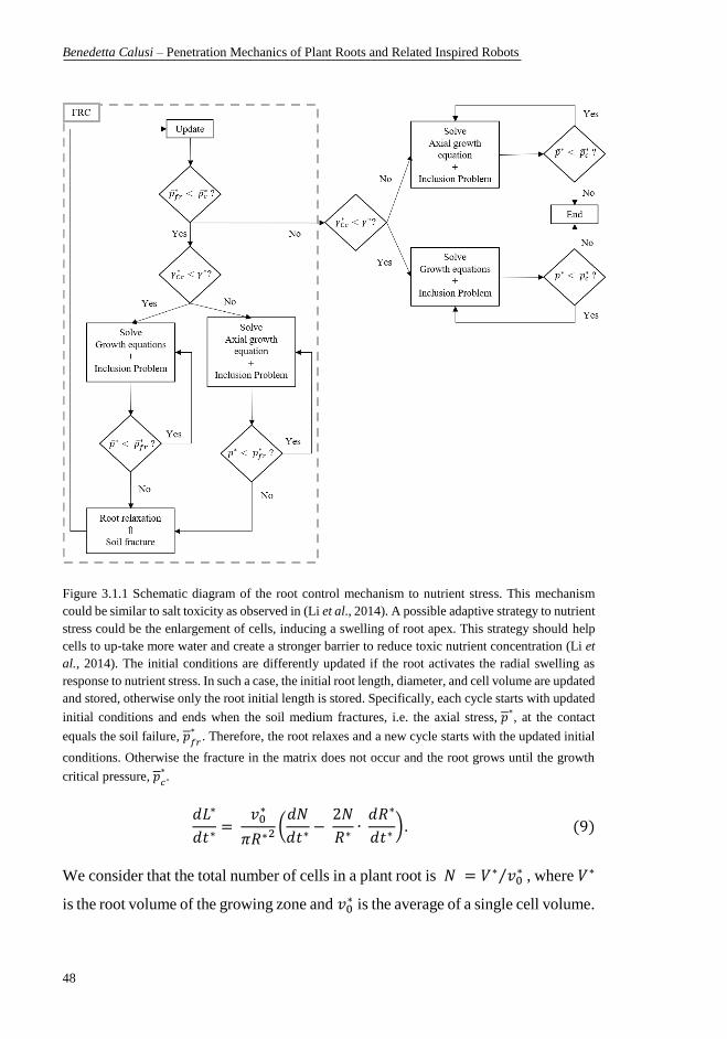
Benedetta Calusi – Penetration Mechanics of Plant Roots and Related Inspired Robots
48
Figure 3.1.1 Schematic diagram of the root control mechanism to nutrient stress. This mechanism
could be similar to salt toxicity as observed in (Li et al., 2014). A possible adaptive strategy to nutrient
stress could be the enlargement of cells, inducing a swelling of root apex. This strategy should help
cells to up-take more water and create a stronger barrier to reduce toxic nutrient concentration (Li et
al., 2014). The initial conditions are differently updated if the root activates the radial swelling as
response to nutrient stress. In such a case, the initial root length, diameter, and cell volume are updated
and stored, otherwise only the root initial length is stored. Specifically, each cycle starts with updated
initial conditions and ends when the soil medium fractures, i.e. the axial stress, 𝑝∗, at the contact
equals the soil failure, 𝑝𝑓𝑟
∗. Therefore, the root relaxes and a new cycle starts with the updated initial
conditions. Otherwise the fracture in the matrix does not occur and the root grows until the growth
critical pressure, 𝑝𝑐
∗.
𝑑𝐿∗
𝑑𝑡∗=
𝑣0∗
𝜋𝑅∗2(𝑑𝑁
𝑑𝑡∗− 2𝑁
𝑅∗∙ 𝑑𝑅∗
𝑑𝑡∗). (9)
We consider that the total number of cells in a plant root is 𝑁 = 𝑉∗ 𝑣0∗⁄ , where 𝑉∗
is the root volume of the growing zone and 𝑣0∗ is the average of a single cell volume.

• Chapter 3 • Theoretical Model
49
We update 𝑣0∗ with the non-dimensional initial root radius at each FRC to indicate
the possible thickening of cells due to the chemical stimulus.
3.1.2. Adimensionalization
We scale the variables by writing
𝐿∗ = 𝐿0∗ 𝐿, 𝑅∗ = 𝑅0
∗𝑅, 𝑡∗ = 𝑡𝑟𝑒𝑓∗ 𝑡,
where 𝐿0∗ represents the length of the growing region from the tip to the end of the
elongation zone and 𝑡𝑟𝑒𝑓∗ is the duration of the experiments. We assume 𝐿0
∗ =
3mm, and 𝑡𝑟𝑒𝑓∗ = 3days as in Chapter 2. We consider for 𝑅0
∗ the values of the top
diameter at the third day of life (the related experimental work has been performed
by IIT).
𝐿1∗ , 𝑅1
∗ represent the initial length and radius of the elastic cylinder, respectively, in
each cycle and we assume zero pressure at both ends of the cycle. Therefore, we
can write
𝐿1∗ = 𝐿0
∗ 𝐿(𝑡0), 𝑅1∗ = 𝑅0
∗𝑅(𝑡0),
where the adimensional length 𝐿(𝑡0) and radius 𝑅(𝑡0) are “updated” at the
beginning of each cycle. By assuming the same length growing zone (from the
meristematic to the elongation region) and number of cells at the beginning of each
FRC with an increasing radius (𝑣0∗𝑁(𝑡0) = 𝜋𝐿
∗(𝑡0)𝑅∗2(𝑡0)), we update the single
cell volume 𝑣0∗ with the non-dimensional initial root radius in each FRC, i.e. 𝑣0
∗ ∝
𝑅2(𝑡0).
Furthermore, by assuming that the root growth ends when �̅�∗ = �̅�𝑐∗ , from the
equation (8.1) we obtain
𝛽∗ = 𝛾∗𝑁𝑐𝜌−1, 𝜌 =
3
4,
where

Benedetta Calusi – Penetration Mechanics of Plant Roots and Related Inspired Robots
50
𝑁𝑐 = 𝑁(𝑡0)1 +
�̅�𝑐𝐸𝑐(𝑈1𝐵1 − 𝑈2𝐴1
𝑈1)
1 −�̅�𝑐𝐸𝑐(𝑈1 − 𝑈2𝑈1
), (10)
and
• 𝑈1 = (1 − 𝜈𝑐)(1 + 𝐴2) ,
• U2 = 2𝜈𝑐2(1 − 𝐴1),
• 𝐴1 = 𝜖2 𝐸𝑐
𝐸𝑚𝜐𝑚
(1−𝜒)(1+𝜐𝑚)
𝜈𝑐(1−𝜐𝑚),
• A2 =𝐸𝑐
𝐸𝑚
(1+𝜐𝑚)
(1−𝜐𝑐)[1 − 𝜖2 +
𝜀2
1−2𝜐𝑚 (2𝜐𝑚
2 (1−𝜒)
1−𝜐𝑚− 1)] ,
• 𝜖 =𝑅1∗
𝑅2∗ , 𝜒 =
𝐿1∗
𝐿2∗ .
In the case of axial growth, the equation (10) corresponds to the equation (7)
Chapter 2.
3.2. Theoretical Results
The theoretical results are performed by means of the equations (8.1) and (8.2)
applied to the growing zone of the root and the related surrounding medium (Figure
2.1.2, Subsection 2.2.1). We suppose that the soil is greater than the root, i.e.
𝑅∗, 𝑅1∗ ≪ 𝑅2
∗ and 𝐿∗, 𝐿1∗ ≪ 𝐿2
∗ (Figure 2.1.2, Chapter 2). Therefore, we set the
values of the parameters 𝜒, 𝑅2∗, 𝑝
𝑐
∗, 𝐸𝑐 , 𝜈𝑚,𝑐 , and 𝜂∗as in Chapter 2. The values used
for the matrix Young modulus, 𝐸𝑚, and the fracture pressure, 𝑝𝑓𝑟∗
, are obtained by
means of compression tests and are reported in Table 1, Section 2.2. The estimated
values of 𝛾∗ for Zea mays roots grown in artificial soil with and without nutrient
are in Table 2.
The four different MS concentrations are labelled MS1, MS2, MS3, and MS4 and
correspond to increasing MS concentration.

• Chapter 3 • Theoretical Results
51
The value of the scaling parameter 𝛾∗ of the input power from the surrounding
matrix increases with both the Phytagel concentration (used in the previous
Chapter) and the MS concentration (only the MS2-Group B and Group C have a
lower estimated value than the corresponding MS1). The results from the equations
(8.1) and (8.2) are given in Figure 3.2.1. Since we have observed that the radial
swelling of 17% at the height of meristematic area occurs in the 5-6-day old roots
for the MS4 concentration with respect to the mature region, we consider the
increase of 17% in the top diameter at the 6-day age for the comparison with the
numerical solutions (the related experimental work has been performed by IIT).
The numerical result of the MS4-Group B is smaller than the measured data for the
same elongation reduction.
Figure 3.2.2-Figure 3.2.4 present the numerical solutions of the MS1-MS3
concentrations. It is worth noting that the equation (8.2) cannot allow a decrease in
root radius, since 𝛾𝐶𝑐∗ represents the parameter related to the energy released by
seed without nutrients in soil and the soil medium is only an external source of
water.
Table 2 Estimated value of the parameter 𝛾∗ related to the nutrient availability. In the control
concentration, i.e. without nutrient in the soil medium, the plant seed furnishes the nutrient for the
growth and is the parameter labelled as 𝛾𝐶𝑐∗ in the current Section.
𝜸∗(MPa mm3 s-1)
Control
conc.
MS1
conc.
MS2
conc.
MS3
conc.
MS4
conc.
Group B (0.3% Phyt.
conc.)
1.94·10-3 2.18·10-3 1.955·10-3 2.531·10-3 3.098·10-3
Group C (0.6% Phyt.
conc.)
2.56·10-3 2.932·10-3 2.666·10-3 2.937·10-3 4.093·10-3
Group D (0.9% Phyt.
conc.)
4.76·10-3 4.783·10-3 5.638·10-3 6.429·10-3 6.888·10-3

Benedetta Calusi – Penetration Mechanics of Plant Roots and Related Inspired Robots
52
Figure 3.2.1 Numerical solution of length (a) and radius (b) evolution and axial (c) and radial (d)
pressure against time. The red circles are the experimental data (mean values ±SD) in MS4
concentration.

• Chapter 3 • Theoretical Results
53
Figure 3.2.2 Numerical solution of length (a) and radius (b) evolution and axial (c) and radial (d)
pressure against time. The red circles are the experimental data (mean values ±SD) in MS1
concentration.
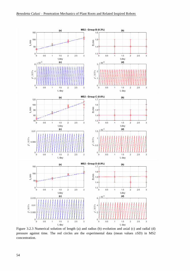
Benedetta Calusi – Penetration Mechanics of Plant Roots and Related Inspired Robots
54
Figure 3.2.3 Numerical solution of length (a) and radius (b) evolution and axial (c) and radial (d)
pressure against time. The red circles are the experimental data (mean values ±SD) in MS2
concentration.
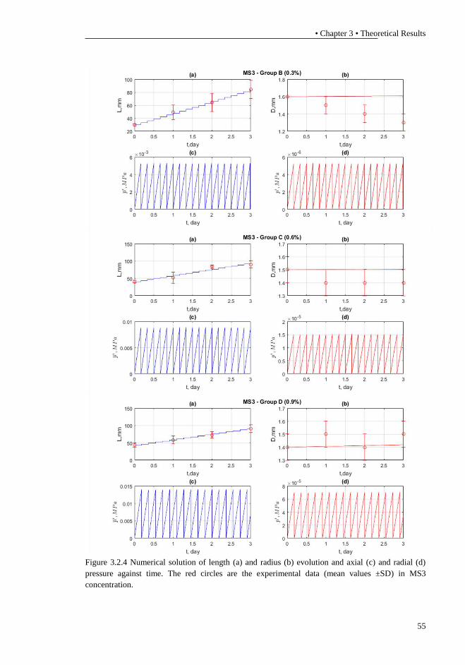
• Chapter 3 • Theoretical Results
55
Figure 3.2.4 Numerical solution of length (a) and radius (b) evolution and axial (c) and radial (d)
pressure against time. The red circles are the experimental data (mean values ±SD) in MS3
concentration.
Benedetta Calusi – Penetration Mechanics of Plant Roots and Related Inspired Robots
56
3.3. Interpretation and Discussion
We observed the behaviour of Zea mays roots in artificial soils with different
nutrient concentrations. Plants grown inside soil media with high concentrations of
nutrients developed shorter and thicker root apparatus. The experiments have been
repeated using soils with three different Phytagel concentrations and, in all the three
cases, the root elongation rate decreased with the increase of nutrient
concentrations.
It was possible to notice a visible enlargement for roots grown in media with higher
concentrations of nutrients. The swelling was localized at the height of the
meristematic area, which was the most sensitive area to the environment changes,
e.g. to salt stress (Huang and van Steveninck, 1990). The experimental data showed
that the excess of Murashige and Skoog Basal Salt Mixture, MS (Murashige and
Skoog, 1962), in soil produces an abnormal radial swelling and elongation
reduction and it can have a similar interpretation to the root swelling, due to NaCl
stress (Li et al., 2014). Therefore, the swelling of root observed in our study in the
presence of MS4 concentration might be a further example of root sensibility to
mineral nutrients stress.
The aim of this study is to couple experimental with theoretical results to gain a
better understanding of how plant roots face nutrient stress. In order to explain such
morphological and strategical adaptation of plant roots, we proposed a growth
model by considering also the mechanical pressure due to the interaction between
the root and the surrounding soil medium. In particular, we modelled the radial
expansion through a critical threshold to describe the radial swelling as found in
the experiments. Therefore, we formulated a hypothesis that the root radial
expansion can be activated in the presence of an excessive nutrient concentration
in the soil medium as an adaptation mechanism of response to nutrient availability.
In fact, the equation (8.2) represents an activation equation for radial growth with
a threshold level for the scaling parameter related to the nutrient availability, 𝛾∗. In
accordance with the experiments, 𝛾∗ increased with the Phytagel and MS

• Chapter 3 • Interpretation and Discussion
57
concentration. Specifically, the decrease in root length and the increase in root
diameter occurred with respect to the increase in the values of 𝛾∗ and MS
concentration in the soil medium for both our analytical and experimental results,
respectively. One of the limits in our modelling approach is the underestimation of
the radial expansion. Nevertheless, there is a significant scope to extend the
theoretical model to incorporate other constitutive equations, e.g. more complex
mechanical properties of root tissues and soil medium, the potential regulation of
hormones and the osmotic effect at cellular level due to the outer medium. Such
factors will be addressed in future studies by measuring further key parameters
under experimental control. This study could lead to deeper investigations into the
root behaviour mechanisms used to convert such adaptive strategies into bio-
inspired approaches.

Benedetta Calusi – Penetration Mechanics of Plant Roots and Related Inspired Robots
58
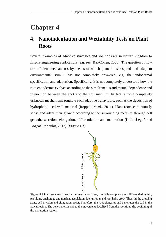
• Chapter 4 • Nanoindentation and Wettability Tests on Plant Roots
59
Chapter 4
4. Nanoindentation and Wettability Tests on Plant
Roots
Several examples of adaptive strategies and solutions are in Nature kingdom to
inspire engineering applications, e.g. see (Bar-Cohen, 2006). The question of how
the efficient mechanisms by means of which plant roots respond and adapt to
environmental stimuli has not completely answered, e.g. the endodermal
specification and adaptation. Specifically, it is not completely understood how the
root endodermis evolves according to the simultaneous and mutual dependence and
interaction between the root and the soil medium. In fact, almost completely
unknown mechanisms regulate such adaptive behaviours, such as the deposition of
hydrophobic cell wall material (Roppolo et al., 2011). Plant roots continuously
sense and adapt their growth according to the surrounding medium through cell
growth, secretion, elongation, differentiation and maturation (Kolb, Legué and
Bogeat-Triboulot, 2017) (Figure 4.1).
Figure 4.1 Plant root structure. In the maturation zone, the cells complete their differentiation and,
providing anchorage and nutrient acquisition, lateral roots and root hairs grow. Then, in the growing
zone, cell division and elongation occur. Therefore, the root elongates and penetrates the soil in the
apical region. The penetration is due to the movements localized from the root tip to the beginning of
the maturation region.

Benedetta Calusi – Penetration Mechanics of Plant Roots and Related Inspired Robots
60
The addition, the growth, and the elongation of new material occur at the apical
zone of the root between the meristematic and the elongation area, allowing the
penetration in the soil. Then, the main differentiation of cells results in the mature
zone with also the onset of hairs and lateral roots. Thus, the growing tip could
control, coordinate and enhance the root system development and ability to face
and withstand the unexpected physical and chemical obstacles. In fact, roots are
extremely smart to resist to chemical and mechanical stimuli during the growth and,
thus, to adjust their penetration direction and ability with a wide range of “active”
responses, e.g. through radial swelling and reduction in elongation due to a toxic
level of salt (Li et al., 2014) and high soil impedance (A. Bengough and Mullins,
1990), respectively. Recent studies remark that plants can be regarded as sensory
and communicative organisms with active problem-solving behaviour, as C.
Darwin and F. Darwin firstly hypothesised in “The power of movement in plants”
(Darwin and Darwin, 1880; Baluška et al., 2009; Gagliano, 2017). In the latter
manuscript a root tip that bends away when is irritated by contact is depicted
(Figure 4.2).
Figure 4.2 (a) “Vicia faba: A, radicle beginning to bend from the attached little square of card; B,
bent at a rectangle; C, bent into a circle or loop, with the tip beginning to bend downwards through
the action of geotropism.” from (Darwin and Darwin, 1880). (b) A Borlotti Lamon bean (Phaseolus
vulgaris L.) exposed to light during growing in a 2D-confinement. The scale bar equals 2000 µm.
(b) (a)
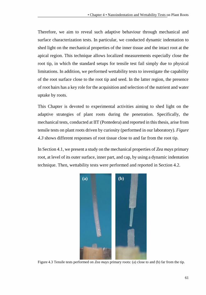
• Chapter 4 • Nanoindentation and Wettability Tests on Plant Roots
61
Therefore, we aim to reveal such adaptive behaviour through mechanical and
surface characterization tests. In particular, we conducted dynamic indentation to
shed light on the mechanical properties of the inner tissue and the intact root at the
apical region. This technique allows localized measurements especially close the
root tip, in which the standard setups for tensile test fail simply due to physical
limitations. In addition, we performed wettability tests to investigate the capability
of the root surface close to the root tip and seed. In the latter region, the presence
of root hairs has a key role for the acquisition and selection of the nutrient and water
uptake by roots.
This Chapter is devoted to experimental activities aiming to shed light on the
adaptive strategies of plant roots during the penetration. Specifically, the
mechanical tests, conducted at IIT (Pontedera) and reported in this thesis, arise from
tensile tests on plant roots driven by curiosity (performed in our laboratory). Figure
4.3 shows different responses of root tissue close to and far from the root tip.
In Section 4.1, we present a study on the mechanical properties of Zea mays primary
root, at level of its outer surface, inner part, and cap, by using a dynamic indentation
technique. Then, wettability tests were performed and reported in Section 4.2.
Figure 4.3 Tensile tests performed on Zea mays primary roots: (a) close to and (b) far from the tip.
(b) (a)

Benedetta Calusi – Penetration Mechanics of Plant Roots and Related Inspired Robots
62
4.1. Dynamic Nanoindentation Tests
4.1.1. Experimental Procedure
The experiments were performed using 3/4-day old Zea mays L. roots. The seeds
were placed on filter paper with tap water and kept into a growth chamber at 25˚C.
We measured the mechanical properties in correspondence of the outer wall and
inner core of the root by dynamic indentation technique in 1-200 Hz frequency
range with an indenter tip of 109 µm and 198.5 µm diameter, employing an iNano
indentation system (Nanomechanics, Inc.). We used a dynamic nanoindentation
technique to measure the storage modulus, E’, and the loss modulus, E’’, i.e. the
real and complex part of the complex modulus which characterizes the material’s
ability to store and damp energy, respectively. E’ provides information about the
material ability to store energy elastically and E’’ gives information about the
material ability to dissipate energy (Pharr, Oliver and Brotzen, 1992; Herbert,
Oliver and Pharr, 2008; Herbert et al., 2009). In fact, E’ and E’’ are related to the
storage stiffness and loss stiffness of the sample, respectively. E’ is comparable to
the Young’s modulus if damping is negligible.
The experiments were carried out in distilled water and were made on roots (we cut
the samples ~1cm in length from the tip) fixed on the bottom of the holder by means
of attack (Loctite) at different distances from the tip (2, 3, 4, 5, 6, and 7 mm) in
correspondence of the wall, the inner core, and the root cap (Figure 4.1.1, Figure
4.1.2). Due to the complex geometry of root tip, an ad hoc sample holder with two
inclinations was built to perform tests in the root tip area (Figure 4.1.1b). In order
to extract the root core, we made a circumferential incision of the root at the base
of the seed, thus the outer wall can be easily separated from the inner core (Figure
4.1.1d). Then, we performed tests by exploiting the indenter tip of 198.5 µm
diameter on both the intact root and the inner core and the indenter tip of 109 µm
diameter near the root cap.
The results and the measurements number of the nanoindentation tests along the
three root regions are reported in Tables 3-5. Figure 4.1.3 and Figure 4.1.4 show
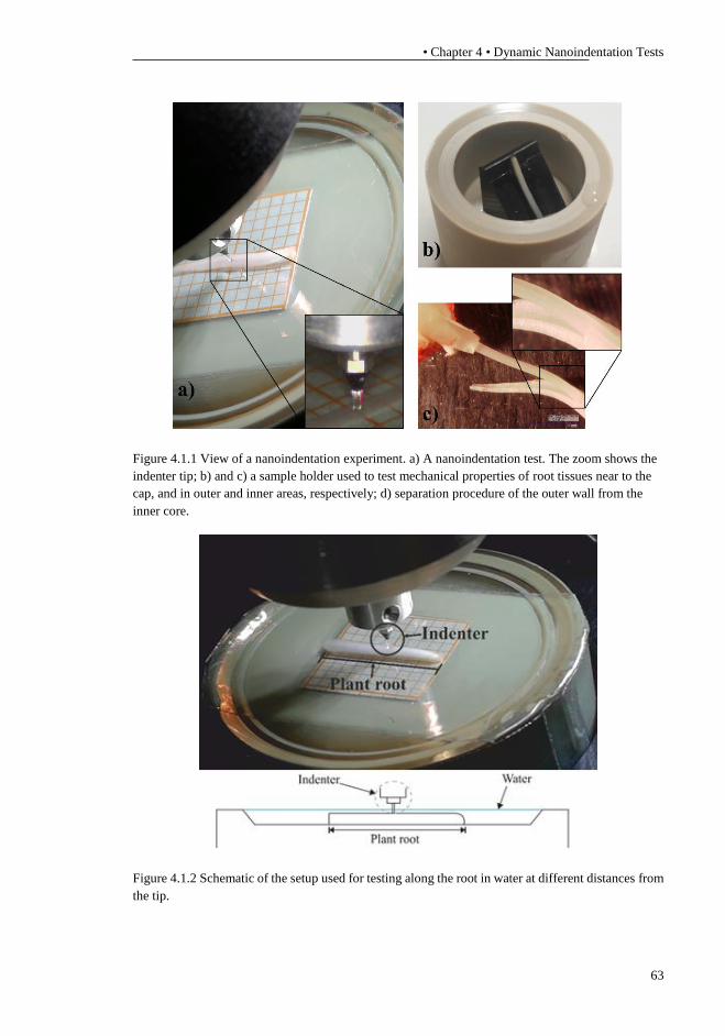
• Chapter 4 • Dynamic Nanoindentation Tests
63
Figure 4.1.1 View of a nanoindentation experiment. a) A nanoindentation test. The zoom shows the
indenter tip; b) and c) a sample holder used to test mechanical properties of root tissues near to the
cap, and in outer and inner areas, respectively; d) separation procedure of the outer wall from the
inner core.
Figure 4.1.2 Schematic of the setup used for testing along the root in water at different distances from
the tip.

Benedetta Calusi – Penetration Mechanics of Plant Roots and Related Inspired Robots
64
graphical results of the storage and loss moduli for both the intact root and the
inner tissue level.
4.1.2. Statistical Analysis
We performed statistical analysis to quantify the storage modulus (E’) and the loss
modulus (E’’) changes with respect to the distance/frequency from the tip and at
different tissue level (i.e. outer and inner tissues) for each frequency/distance.
The most appropriate statistical method is the ANOVA test in order to assess the
statistical significance of the different response in the measurement of the moduli
depending on the distance from the tip, frequency and tissue level. This test assumes
that the data in the groups at various levels of effects are normally distributed,
statistically independent and have the same variance. However, since our data
showed some deviations from normality and/or homoscedasticity, we also
performed different statistical tests when appropriated: the non-parametric Kruskal-
Wallis test when the normality assumption failed, the Welch test when the data
showed a strong heteroscedasticity.
In this regard, we exploited the Kruskal-Wallis test and the Welch test to verify the
significance of the storage and loss modulus measurements, respectively, at both
the intact root and inner core. We used the one-way ANOVA to test the significance
of the measurements near the cap for both the storage and loss moduli.
The statistical analysis is at the 95% confidence level and performed in R.
We obtained significant E’ difference with respect to distance from the tip (2mm-
5mm) for each frequency for both intact root and inner tissue level (Table 6). While,
we had significant E’ differences with respect to frequency for each distance, except
for the inner core at 2mm and 3mm from the tip and for the intact root at 2mm,
5mm and 7mm from the tip (p > 0.05, Table 7).
In addition, the results of the Welch tests showed significant E’’ difference with
respect to distances from the tip (2mm-7mm) for intact root at each frequency and
(2-5mm) for inner tissue at 1-35Hz (Table 8). Moreover, the measurements of E’’
changes are significant with respect to the frequency influence at both intact root

• Chapter 4 • Dynamic Nanoindentation Tests
65
and inner core at each distance from the tip, except for the inner core at 2mm-3mm
and for the intact root at 7mm (p > 0.05, Table 9).
The one-way ANOVA results pointed out significant E’ and E’’ differences near
the root cap with respect to the frequency (Table 10).
Table 3. Storage and loss moduli (mean value ± SD) of the root cap for all frequencies (1, 3, 10, 15,
35, 85, 200 Hz). A total of 7 indentations on 4 roots were performed.
Freq. (Hz) E’ (MPa) E’’ (MPa)
200 4.23±1.53 0.61±0.22
85 3.9±1.29 0.6±0.22
35 3.65±1.22 0.56±0.18
15 3.39±1.15 0.55±0.17
10 3.27±1.13 0.55±0.16
3 2.81±1.01 0.54±0.17
1 2.49±0.93 0.55±0.2
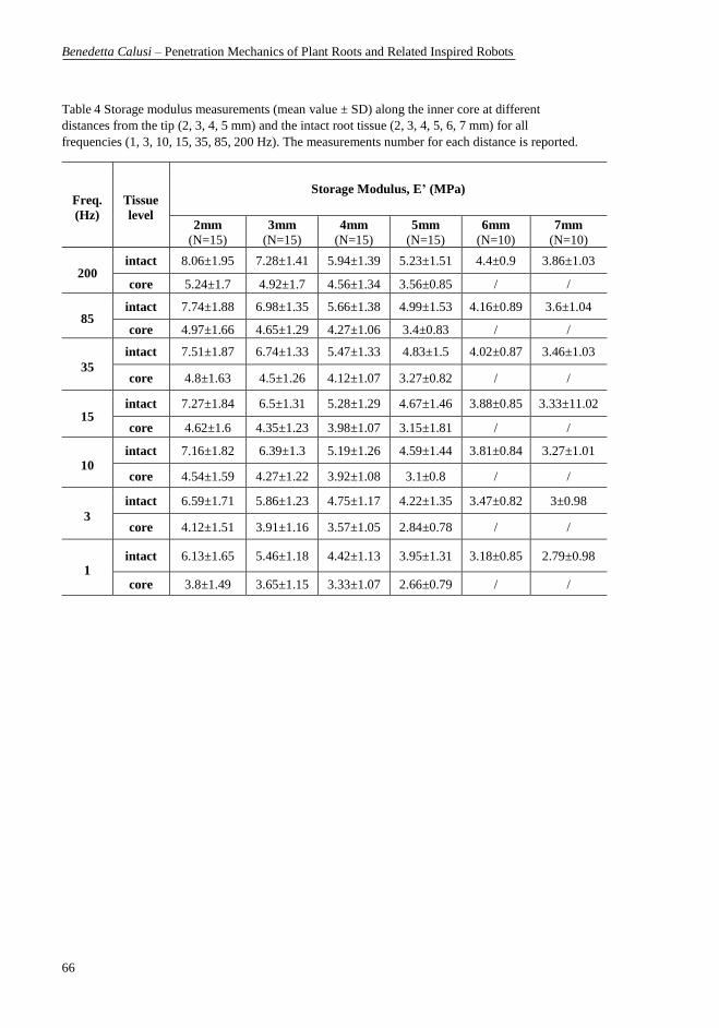
Benedetta Calusi – Penetration Mechanics of Plant Roots and Related Inspired Robots
66
Table 4 Storage modulus measurements (mean value ± SD) along the inner core at different
distances from the tip (2, 3, 4, 5 mm) and the intact root tissue (2, 3, 4, 5, 6, 7 mm) for all
frequencies (1, 3, 10, 15, 35, 85, 200 Hz). The measurements number for each distance is reported.
Freq.
(Hz)
Tissue
level
Storage Modulus, E’ (MPa)
2mm
(N=15)
3mm
(N=15)
4mm
(N=15)
5mm
(N=15)
6mm
(N=10)
7mm
(N=10)
200 intact 8.06±1.95 7.28±1.41 5.94±1.39 5.23±1.51 4.4±0.9 3.86±1.03
core 5.24±1.7 4.92±1.7 4.56±1.34 3.56±0.85 / /
85 intact 7.74±1.88 6.98±1.35 5.66±1.38 4.99±1.53 4.16±0.89 3.6±1.04
core 4.97±1.66 4.65±1.29 4.27±1.06 3.4±0.83 / /
35
intact 7.51±1.87 6.74±1.33 5.47±1.33 4.83±1.5 4.02±0.87 3.46±1.03
core 4.8±1.63 4.5±1.26 4.12±1.07 3.27±0.82 / /
15 intact 7.27±1.84 6.5±1.31 5.28±1.29 4.67±1.46 3.88±0.85 3.33±11.02
core 4.62±1.6 4.35±1.23 3.98±1.07 3.15±1.81 / /
10
intact 7.16±1.82 6.39±1.3 5.19±1.26 4.59±1.44 3.81±0.84 3.27±1.01
core 4.54±1.59 4.27±1.22 3.92±1.08 3.1±0.8 / /
3
intact 6.59±1.71 5.86±1.23 4.75±1.17 4.22±1.35 3.47±0.82 3±0.98
core 4.12±1.51 3.91±1.16 3.57±1.05 2.84±0.78 / /
1 intact 6.13±1.65 5.46±1.18 4.42±1.13 3.95±1.31 3.18±0.85 2.79±0.98
core 3.8±1.49 3.65±1.15 3.33±1.07 2.66±0.79 / /

• Chapter 4 • Dynamic Nanoindentation Tests
67
Table 5 Loss modulus measurements (mean value ± SD) along the inner core at different distances
from the tip (2, 3, 4, 5 mm) and the intact root tissue (2, 3, 4, 5, 6, 7 mm) for all frequencies (1, 3,
10, 15, 35, 85, 200 Hz). The measurements number for each distance is reported.
Freq.
(Hz)
Tissue
level
Loss Modulus, E’’ (MPa)
2mm
(N=15)
3mm
(N=15)
4mm
(N=15)
5mm
(N=15)
6mm
(N=10)
7mm
(N=10)
200 intact 0.49±0.07 0.48±0.08 0.42±0.12 0.34±0.1 0.34±0.09 0.34±0.07
core 0.37± 0.12 0.36±0.12 0.36±0.08 0.3±0.09 / /
85 intact 0.48±0.08 0.47±0.08 0.39±0.09 0.33±0.09 0.30±0.07 0.3±0.07
core 0.35±0.12 0.33±0.1 0.31±0.07 0.26±0.07 / /
35
intact 0.49±0.09 0.47±0.09 0.38±0.09 0.32±0.08 0.29±0.06 0.28±0.06
core 0.35±0.11 0.31±0.1 0.3±0.06 0.25±0.06 / /
15 intact 0.51±0.11 0.49±0.09 0.4±0.09 0.34±0.09 0.3±0.067 0.27±0.05
core 0.37±0.12 0.31±0.1 0.3±0.07 0.25±0.05 / /
10
intact 0.54±0.13 0.51±0.1 0.42±0.1 0.35±0.1 0.32±0.07 0.27±0.05
core 0.38±0.14 0.32±0.1 0.31±0.07 0.26±0.05 / /
3
intact 0.65±0.19 0.59±0.15 0.47±0.12 0.4±0.11 0.38±0.1 0.29±0.08
core 0.44±0.18 0.36±0.11 0.38±0.12 0.28±0.04 / /
1 intact 0.86±0.28 0.73±0.23 0.56±0.16 0.47±0.12 0.46±0.11 0.34±0.12
core 0.48±0.2 0.39±0.12 0.39±0.01 0.3±0.03 / /
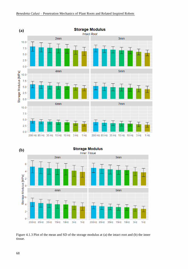
Benedetta Calusi – Penetration Mechanics of Plant Roots and Related Inspired Robots
68
Figure 4.1.3 Plot of the mean and SD of the storage modulus at (a) the intact root and (b) the inner
tissue.
(a)
(b)
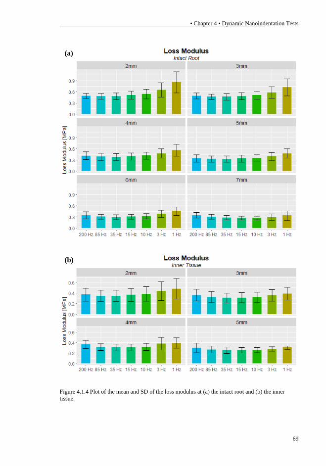
• Chapter 4 • Dynamic Nanoindentation Tests
69
Figure 4.1.4 Plot of the mean and SD of the loss modulus at (a) the intact root and (b) the inner
tissue.
(a)
(b)

Benedetta Calusi – Penetration Mechanics of Plant Roots and Related Inspired Robots
70
Table 6 Results of the Kruskal-Wallis test for the significance of the measurements of E’ obtained at
inner and intact root outer tissue levels for each frequency at the distances of 2, 3, 4 and 5mm from
the tip (df= degrees of freedom).
Tissue Freq. Kruskal-Wallis test: Storage Modulus (E’) vs Distance
Inner tissue
200Hz Kruskal-Wallis chi-squared = 12.14, df = 3, p-value = 0.006918
85Hz Kruskal-Wallis chi-squared = 10.922, df = 3, p-value = 0.01215
35Hz Kruskal-Wallis chi-squared = 11.256, df = 3, p-value = 0.01042
15Hz Kruskal-Wallis chi-squared = 10.862, df = 3, p-value = 0.0125
10Hz Kruskal-Wallis chi-squared = 10.803, df = 3, p-value = 0.01284
3Hz Kruskal-Wallis chi-squared = 9.6728, df = 3, p-value = 0.02156
1Hz Kruskal-Wallis chi-squared = 7.8297, df = 3, p-value = 0.04966
Intact root
200Hz Kruskal-Wallis chi-squared = 19.288, df = 3, p-value = 0.0002384
85Hz Kruskal-Wallis chi-squared = 19.455, df = 3, p-value = 0.0002202
35Hz Kruskal-Wallis chi-squared = 19.255, df = 3, p-value = 0.0002421
15Hz Kruskal-Wallis chi-squared = 18.938, df = 3, p-value = 0.0002815
10Hz Kruskal-Wallis chi-squared = 18.642, df = 3, p-value = 0.0003241
3Hz Kruskal-Wallis chi-squared = 18.242, df = 3, p-value = 0.0003921
1Hz Kruskal-Wallis chi-squared = 16.844, df = 3, p-value = 0.0007609
Table 7 Results of the Kruskal-Wallis test for the significance of the measurements of E’ obtained at
inner and intact root outer tissue levels for each distance from the tip at all the frequencies 200, 85,
35, 15, 10, 3, 1Hz (df= degrees of freedom).
Tissue Dist. Kruskal-Wallis test: Storage Modulus (E’) vs Frequency
Inner tissue
2mm Kruskal-Wallis chi-squared = 12.128, df = 6, p-value = 0.05918
3mm Kruskal-Wallis chi-squared = 10.091, df = 6, p-value = 0.1209
4mm Kruskal-Wallis chi-squared = 14.486, df = 6, p-value = 0.02465
5mm Kruskal-Wallis chi-squared = 14.025, df = 6, p-value = 0.02936
Intact root
2mm Kruskal-Wallis chi-squared = 10.452, df = 6, p-value = 0.1069
3mm Kruskal-Wallis chi-squared = 25.825, df = 6, p-value = 0.0002399
4mm Kruskal-Wallis chi-squared = 13.416, df = 6, p-value = 0.03688
5mm Kruskal-Wallis chi-squared = 11.629, df = 6, p-value = 0.07078
6mm Kruskal-Wallis chi-squared = 12.805, df = 6, p-value = 0.04624
7mm Kruskal-Wallis chi-squared = 9.5971, df = 6, p-value = 0.1427
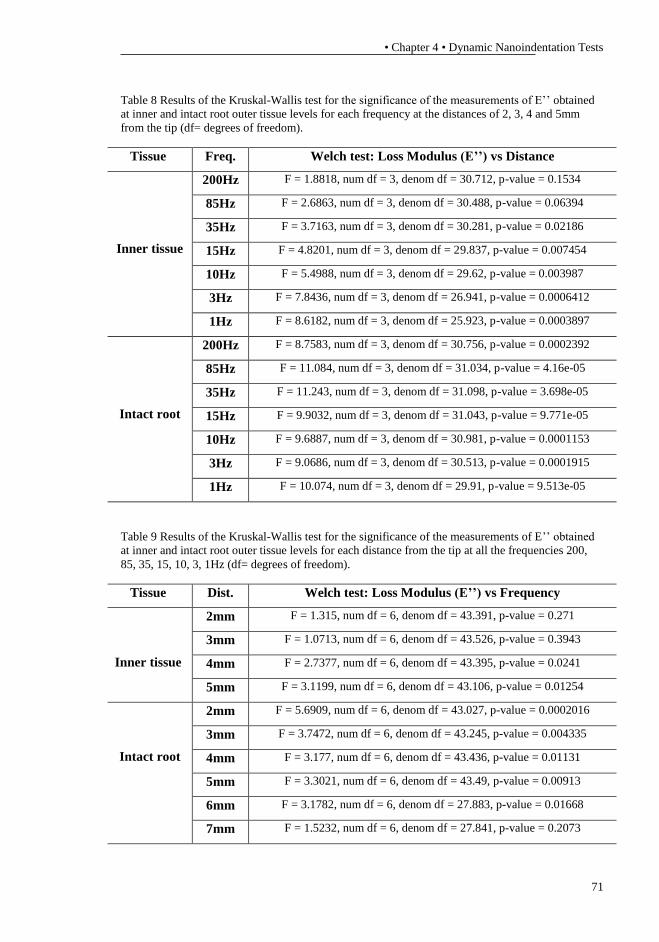
• Chapter 4 • Dynamic Nanoindentation Tests
71
Table 8 Results of the Kruskal-Wallis test for the significance of the measurements of E’’ obtained
at inner and intact root outer tissue levels for each frequency at the distances of 2, 3, 4 and 5mm
from the tip (df= degrees of freedom).
Tissue Freq. Welch test: Loss Modulus (E’’) vs Distance
Inner tissue
200Hz F = 1.8818, num df = 3, denom df = 30.712, p-value = 0.1534
85Hz F = 2.6863, num df = 3, denom df = 30.488, p-value = 0.06394
35Hz F = 3.7163, num df = 3, denom df = 30.281, p-value = 0.02186
15Hz F = 4.8201, num df = 3, denom df = 29.837, p-value = 0.007454
10Hz F = 5.4988, num df = 3, denom df = 29.62, p-value = 0.003987
3Hz F = 7.8436, num df = 3, denom df = 26.941, p-value = 0.0006412
1Hz F = 8.6182, num df = 3, denom df = 25.923, p-value = 0.0003897
Intact root
200Hz F = 8.7583, num df = 3, denom df = 30.756, p-value = 0.0002392
85Hz F = 11.084, num df = 3, denom df = 31.034, p-value = 4.16e-05
35Hz F = 11.243, num df = 3, denom df = 31.098, p-value = 3.698e-05
15Hz F = 9.9032, num df = 3, denom df = 31.043, p-value = 9.771e-05
10Hz F = 9.6887, num df = 3, denom df = 30.981, p-value = 0.0001153
3Hz F = 9.0686, num df = 3, denom df = 30.513, p-value = 0.0001915
1Hz F = 10.074, num df = 3, denom df = 29.91, p-value = 9.513e-05
Table 9 Results of the Kruskal-Wallis test for the significance of the measurements of E’’ obtained
at inner and intact root outer tissue levels for each distance from the tip at all the frequencies 200,
85, 35, 15, 10, 3, 1Hz (df= degrees of freedom).
Tissue Dist. Welch test: Loss Modulus (E’’) vs Frequency
Inner tissue
2mm F = 1.315, num df = 6, denom df = 43.391, p-value = 0.271
3mm F = 1.0713, num df = 6, denom df = 43.526, p-value = 0.3943
4mm F = 2.7377, num df = 6, denom df = 43.395, p-value = 0.0241
5mm F = 3.1199, num df = 6, denom df = 43.106, p-value = 0.01254
Intact root
2mm F = 5.6909, num df = 6, denom df = 43.027, p-value = 0.0002016
3mm F = 3.7472, num df = 6, denom df = 43.245, p-value = 0.004335
4mm F = 3.177, num df = 6, denom df = 43.436, p-value = 0.01131
5mm F = 3.3021, num df = 6, denom df = 43.49, p-value = 0.00913
6mm F = 3.1782, num df = 6, denom df = 27.883, p-value = 0.01668
7mm F = 1.5232, num df = 6, denom df = 27.841, p-value = 0.2073
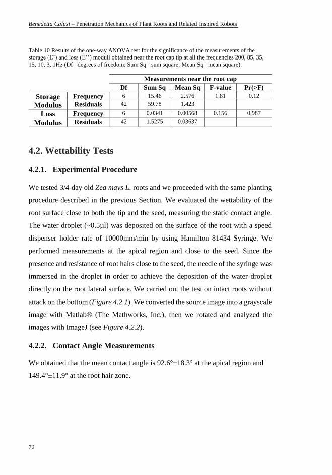
Benedetta Calusi – Penetration Mechanics of Plant Roots and Related Inspired Robots
72
Table 10 Results of the one-way ANOVA test for the significance of the measurements of the
storage (E’) and loss (E’’) moduli obtained near the root cap tip at all the frequencies 200, 85, 35,
15, 10, 3, 1Hz (Df= degrees of freedom; Sum Sq= sum square; Mean Sq= mean square).
Measurements near the root cap
Df Sum Sq Mean Sq F-value Pr(>F)
Storage
Modulus
Frequency 6 15.46 2.576 1.81 0.12
Residuals 42 59.78 1.423
Loss
Modulus
Frequency 6 0.0341 0.00568 0.156 0.987
Residuals 42 1.5275 0.03637
4.2. Wettability Tests
4.2.1. Experimental Procedure
We tested 3/4-day old Zea mays L. roots and we proceeded with the same planting
procedure described in the previous Section. We evaluated the wettability of the
root surface close to both the tip and the seed, measuring the static contact angle.
The water droplet (~0.5µl) was deposited on the surface of the root with a speed
dispenser holder rate of 10000mm/min by using Hamilton 81434 Syringe. We
performed measurements at the apical region and close to the seed. Since the
presence and resistance of root hairs close to the seed, the needle of the syringe was
immersed in the droplet in order to achieve the deposition of the water droplet
directly on the root lateral surface. We carried out the test on intact roots without
attack on the bottom (Figure 4.2.1). We converted the source image into a grayscale
image with Matlab® (The Mathworks, Inc.), then we rotated and analyzed the
images with ImageJ (see Figure 4.2.2).
4.2.2. Contact Angle Measurements
We obtained that the mean contact angle is 92.6°±18.3° at the apical region and
149.4°±11.9° at the root hair zone.
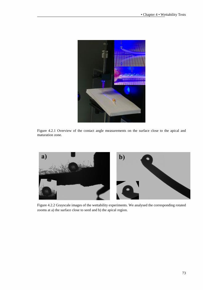
• Chapter 4 • Wettability Tests
73
Figure 4.2.1 Overview of the contact angle measurements on the surface close to the apical and
maturation zone.
Figure 4.2.2 Grayscale images of the wettability experiments. We analysed the corresponding rotated
zooms at a) the surface close to seed and b) the apical region.
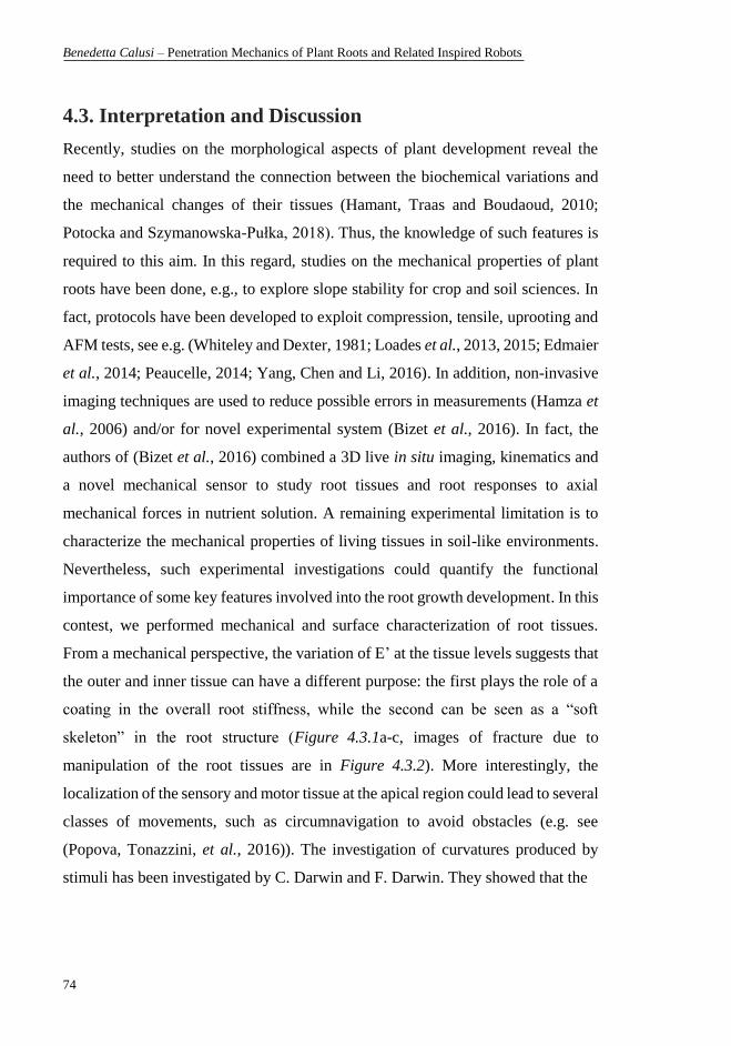
Benedetta Calusi – Penetration Mechanics of Plant Roots and Related Inspired Robots
74
4.3. Interpretation and Discussion
Recently, studies on the morphological aspects of plant development reveal the
need to better understand the connection between the biochemical variations and
the mechanical changes of their tissues (Hamant, Traas and Boudaoud, 2010;
Potocka and Szymanowska-Pułka, 2018). Thus, the knowledge of such features is
required to this aim. In this regard, studies on the mechanical properties of plant
roots have been done, e.g., to explore slope stability for crop and soil sciences. In
fact, protocols have been developed to exploit compression, tensile, uprooting and
AFM tests, see e.g. (Whiteley and Dexter, 1981; Loades et al., 2013, 2015; Edmaier
et al., 2014; Peaucelle, 2014; Yang, Chen and Li, 2016). In addition, non-invasive
imaging techniques are used to reduce possible errors in measurements (Hamza et
al., 2006) and/or for novel experimental system (Bizet et al., 2016). In fact, the
authors of (Bizet et al., 2016) combined a 3D live in situ imaging, kinematics and
a novel mechanical sensor to study root tissues and root responses to axial
mechanical forces in nutrient solution. A remaining experimental limitation is to
characterize the mechanical properties of living tissues in soil-like environments.
Nevertheless, such experimental investigations could quantify the functional
importance of some key features involved into the root growth development. In this
contest, we performed mechanical and surface characterization of root tissues.
From a mechanical perspective, the variation of E’ at the tissue levels suggests that
the outer and inner tissue can have a different purpose: the first plays the role of a
coating in the overall root stiffness, while the second can be seen as a “soft
skeleton” in the root structure (Figure 4.3.1a-c, images of fracture due to
manipulation of the root tissues are in Figure 4.3.2). More interestingly, the
localization of the sensory and motor tissue at the apical region could lead to several
classes of movements, such as circumnavigation to avoid obstacles (e.g. see
(Popova, Tonazzini, et al., 2016)). The investigation of curvatures produced by
stimuli has been investigated by C. Darwin and F. Darwin. They showed that the

• Chapter 4 • Interpretation and Discussion
75
Figure 4.3.1 A 3/4-day old Zea mays L. root, scale bar: 5mm. (a) The apical zone is the most sensitive
region of the root. Cell division and elongation occur at the apical region and allow the root to move
and grow into the soil. The cell division is slower in the quiescent centre, then the cells mainly elongate
and differentiate in the elongation zone. The root cap has the role of protection from the surrounding
soil; (b) Fracture of the outer wall and intact inner core; (c) Twist of the inner core; (d) Water and
nutrients can move across the root through different internal pathways: Apoplast, Transmembrane,
and Symplast pathways. In this regard, the Casparian strip is in the Apoplast pathway, limiting the
water and solute movement due to the presence of suberin (image from (Taiz and Zeiger, 1991)).
The scale bar equals 1000µm in a-c.
sensitiveness of tip transmits the curvature movement to the upper part starting
from 6 mm from the tip (Darwin and Darwin, 1880). In this regard, the mechanism
of root curvature can be allowed due to the increase of softness with the increase of
the distance from the tip (Table 4). Moreover, the authors of (Bizet et al., 2016)
show the presence of mechanical weakness for bending between the growing and
the mature zones in poplar roots during the growth in nutrient solution. In addition,
by comparing the second moment of inertia of a solid and a hollow cylindrical beam
(𝐼𝑠 and 𝐼𝐻, respectively) representing the inner and outer tissues (in similar way of
(Niklas, 1999)), it holds
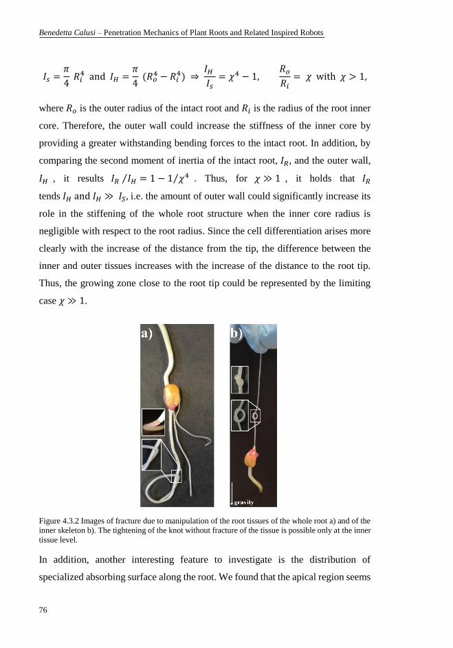
Benedetta Calusi – Penetration Mechanics of Plant Roots and Related Inspired Robots
76
𝐼𝑠 =𝜋
4 𝑅𝑖4 and 𝐼𝐻 =
𝜋
4 (𝑅𝑜
4 − 𝑅𝑖4) ⇒
𝐼𝐻
𝐼𝑠= 𝜒4 − 1,
𝑅𝑜𝑅𝑖= 𝜒 with 𝜒 > 1,
where 𝑅𝑜 is the outer radius of the intact root and 𝑅𝑖 is the radius of the root inner
core. Therefore, the outer wall could increase the stiffness of the inner core by
providing a greater withstanding bending forces to the intact root. In addition, by
comparing the second moment of inertia of the intact root, 𝐼𝑅, and the outer wall,
𝐼𝐻 , it results 𝐼𝑅 𝐼𝐻⁄ = 1 − 1 𝜒4⁄ . Thus, for 𝜒 ≫ 1 , it holds that 𝐼𝑅
tends 𝐼𝐻 and 𝐼𝐻 ≫ 𝐼𝑆, i.e. the amount of outer wall could significantly increase its
role in the stiffening of the whole root structure when the inner core radius is
negligible with respect to the root radius. Since the cell differentiation arises more
clearly with the increase of the distance from the tip, the difference between the
inner and outer tissues increases with the increase of the distance to the root tip.
Thus, the growing zone close to the root tip could be represented by the limiting
case 𝜒 ≫ 1.
Figure 4.3.2 Images of fracture due to manipulation of the root tissues of the whole root a) and of the
inner skeleton b). The tightening of the knot without fracture of the tissue is possible only at the inner
tissue level.
In addition, another interesting feature to investigate is the distribution of
specialized absorbing surface along the root. We found that the apical region seems
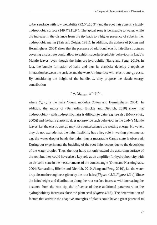
• Chapter 4 • Interpretation and Discussion
77
to be a surface with low wettability (92.6°±18.3°) and the root hair zone is a highly
hydrophobic surface (149.4°±11.9°). The apical zone is permeable to water, while
the increase in the distance from the tip leads to a higher presence of suberin, i.e.
hydrophobic matter (Taiz and Zeiger, 1991). In addition, the authors of (Otten and
Herminghaus, 2004) show that the presence of additional elastic hair-like structures
covering a substrate could allow to exhibit superhydrophobic behaviour in Lady’s
Mantle leaves, even though the hairs are hydrophilic (Jiang and Feng, 2010). In
fact, the bundle formation of hairs and thus its elasticity develop a repulsive
interaction between the surface and the water/air interface with elastic energy costs.
By considering the height of the bundle, h, they propose the elastic energy
contribution
Γ ∝ (𝐸ℎ𝑎𝑖𝑟𝑠 ∙ ℎ−1)1 2⁄ ,
where 𝐸ℎ𝑎𝑖𝑟𝑠 is the hairs Young modulus (Otten and Herminghaus, 2004). In
addition, the author of (Bernardino, Blickle and Dietrich, 2010) show that
hydrophobicity with hydrophilic hairs is difficult to gain (e.g. see also (Mock et al.,
2005)) and the hairs elasticity does not provide such behaviour in the Lady’s Mantle
leaves, i.e. the elastic energy may not counterbalance the wetting energy. However,
they do not exclude that the hairs flexibility has a key role in wetting phenomena,
e.g. the water droplet bends the hairs, thus a metastable Cassie state is observed.
During our experiments the buckling of the root hairs occurs due to the deposition
of the water droplet. Thus, the root hairs not only extend the absorbing surface of
the root but they could have also a key role as an amplifier for hydrophobicity with
an air-solid state in the measurements of the contact angle (Otten and Herminghaus,
2004; Bernardino, Blickle and Dietrich, 2010; Jiang and Feng, 2010), i.e. the water
drop sits on the roughness given by the root hairs (Figure 4.3.3, Figure 4.3.4). Since
the hairs height and distribution along the root surface increase with increasing the
distance from the root tip, the influence of these additional parameters on the
hydrophobicity increases close the plant seed (Figure 4.3.5). The determination of
factors that activate the adaptive strategies of plants could have a great potential to
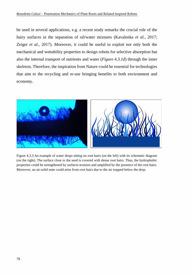
Benedetta Calusi – Penetration Mechanics of Plant Roots and Related Inspired Robots
78
be used in several applications, e.g. a recent study remarks the crucial role of the
hairy surfaces in the separation of oil/water mixtures (Kavalenka et al., 2017;
Zeiger et al., 2017). Moreover, it could be useful to exploit not only both the
mechanical and wettability properties to design robots for selective absorption but
also the internal transport of nutrients and water (Figure 4.3.1d) through the inner
skeleton. Therefore, the inspiration from Nature could be essential for technologies
that aim to the recycling and re-use bringing benefits to both environment and
economy.
Figure 4.3.3 An example of water drops sitting on root hairs (on the left) with its schematic diagram
(on the right). The surface close to the seed is covered with dense root hairs. Thus, the hydrophobic
properties could be strengthened by surfaces textures and amplified by the presence of the root hairs.
Moreover, an air-solid state could arise from root hairs due to the air trapped below the drop.
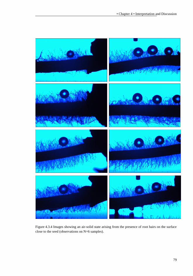
• Chapter 4 • Interpretation and Discussion
79
Figure 4.3.4 Images showing an air-solid state arising from the presence of root hairs on the surface
close to the seed (observations on N=6 samples).

Benedetta Calusi – Penetration Mechanics of Plant Roots and Related Inspired Robots
80
Figure 4.3.5 Droplets with different shapes along a plant root due to the variation of the height and
distribution of hairs on the root surface.
• Chapter 5 • Plant Roots Growth in Photoelastic Gelatine
81
Chapter 5
5. Plant Roots Growth in Photoelastic Gelatine
Plant roots represent an excellent example of successful soil penetration and
exploration strategies (Popova, van Dusschoten, et al., 2016). Roots can efficiently
penetrate the substrate and perform key functions for growth and survival (Gilroy
and Masson, 2008). Since the mechanical properties of the growth medium
influence the plant root growth, the interest on the development of non-invasively
technique to observe root growth is increasing (Kolb, Hartmann and Genet, 2012;
Silverberg et al., 2012; Tan et al., 2015; Keyes et al., 2016; Popova, van
Dusschoten, et al., 2016; Zha et al., 2016). Because of its transparency, artificial
substrates, e.g. agar and hydrogel, are mainly adopted to directly observe the root
growth (Silverberg et al., 2012; Tan et al., 2015; Zha et al., 2016). In addition, the
development of novel non-invasive imaging techniques has a high significance to
capture a more complete feedback between roots development and soil properties,
see e.g. (Keyes et al., 2016; Popova, van Dusschoten, et al., 2016; Colombi et al.,
2017). In fact, in (Popova, van Dusschoten, et al., 2016) a novel 3-D imaging
technique, MRI, to dynamically and non–invasively investigate the influence of
physical soil properties on root growth in non–transparent media has been
developed. Photoelasticity can be a further powerful technique to observe the
penetration strategies of plant roots. Photoelastic stress analysis is a technique once
widely employed by engineers to observe stress patterns (Durelli and Riley, 1965).
Moreover, the use of photoelasticity have been used also to visualize and analyse
the strain in medical applications, see e.g. (Tomlinson and Taylor, 2015). In
(Tomlinson and Taylor, 2015) gelatine mixed with glycerin was used for the
photoelastic tests as a starting point for needle insertion. In early works forces
exerted by moving organisms have been quantitatively measured by means of
photoelasticity, e.g. (Harris, 1978; Full, Yamauchi and Jindrich, 1995; Goldman
and Hu, 2010; Hu, David and Shelley, 2012; Dorgan, Law and Rouse, 2013;

Benedetta Calusi – Penetration Mechanics of Plant Roots and Related Inspired Robots
82
Mirbagheri et al., 2015). This technique is non-invasive and requires minimal
equipment for both dynamic measurements of forces exerted by moving organisms
(Harris, 1978) and direct observation of the phenomenon. In fact, gelatine has been
used to study animals locomotion, e.g. in (Dorgan, Arwade and Jumars, 2007)
gelatine mimics muddy sediments. Nonetheless, the photoelastic technique is also
applied to living organisms in granular substrates (Kolb, Hartmann and Genet,
2012; Wendell et al., 2012; Mirbagheri et al., 2015). Previous studies on plant root
growth have exploited photoelastic soils by means of granular systems where
photoelastic grains are used to visualize and quantify the local forces in the system
(Kolb, Hartmann and Genet, 2012; Wendell et al., 2012). This Chapter describes
the application of photoelasticity to the plant root growth in photoelastic
homogeneous medium. When small forces are exerted, small stresses can be
generated, thus only low fringe orders can be seen as in the case of plant root
growth. Therefore, we exploited the fringe multiplication applied to the study of
plant roots growing in edible gelatine. The fringe multiplication technique is
especially useful for increasing the observable fringe orders. In fact, D. Post
demonstrated the potential of the fringe multiplier, which consists of two partial
mirrors at the front and rear of the specimen into a traditional polariscope (see e.g.
(Post, 1955, 1966, 1970)). Fringe multiplication is a full-field compensation
technique where the fringe fractional orders can be estimated simultaneously at all
points on the sample (Dally and Riley, 1991). This technique may provide further
insights into the forces exerted during root growing and bending. Since plant roots
have great ability to explore and respond to environmental stimuli, a root-like
growing device represents a translation of biological concepts into an engineering
system not only for soil penetration but also for biomedical applications. In fact,
the needle insertion (e.g. epidural puncture), guidance problems deep in the body
require relatively large distance to be travelled, to penetrate and to be in close
contact with tissues with different layer properties (e.g. from a hard to a soft layer).
Minimally invasive penetrations may be achieved by controlling feed position or
velocity using a highly sensitised tip as analogue of root tip to detect mechanical

• Chapter 5 • Photoelasticity
83
properties of the surrounding medium. Therefore, a microdrilling that adapts to the
surrounding environment and is able to avoid obstacles offers potential for
improved surgery in areas of difficult access (Brett et al., 1995).
5.1. Photoelasticity
We report a brief description of the photoelasticity principles in this Section and
fringe multiplication in Section 5.2. For more details on the theory about
photoelastic techniques we refer the reader to e.g. the book Experimental Stress
Analysis by Dally and Riley (Dally and Riley, 1991).
Light propagates in free space with a velocity, 𝑐, approximately of 3 × 10⁸𝑚/𝑠
and in any other bodies with a lower velocity, 𝑣 . The ratio between the two
velocities is called index of refraction, 𝑛 = 𝑐 𝑣⁄ . When a ray of light enters in
optically isotropic materials, the refractive index does not depend upon the
direction of propagation or the plane of vibration. While optically anisotropic
bodies have different indices of refraction in each of the two mutually-
perpendicular planes in which the light may vibrate. Such materials are named
birefringent. It is possible to obtain a temporary or artificial birefringence in certain
bodies. In fact, many non-crystalline transparent materials are ordinarily optically
isotropic and become anisotropic only during the application of external forces, i.e.
it is temporarily birefringent. Such materials have photoelastic behaviour and are
called photoelastic materials.
When a polarized light4 pass through the body of thickness h, and it is divided into
two components rays that are linearly polarized at right angles to each other,
propagating with different velocities. Therefore, the relative retardation between
the two rays is
4 A polarized light emits waves in which the vibrations occur in a single plane. While, an
ordinary light source emits waves that are vibrating in more than one plane (e.g. the light
emitted by the sun and by a lamp).

Benedetta Calusi – Penetration Mechanics of Plant Roots and Related Inspired Robots
84
𝛿 = 𝑐 (ℎ
𝑣1+
ℎ
𝑣2) = ℎ(𝑛1 − 𝑛2),
where ℎ/𝑣𝑖 = 𝑡𝑖 is the time necessary of the i-th ray to cross the body, 𝑣𝑖 , 𝑛𝑖
represent the velocity of propagation and the refractive index of the i-th ray,
respectively, with i =1, 2. Thus, the phase difference of the light components
emerging is given by
∆=2𝜋
𝜆 (𝑡2 − 𝑡1) =
2𝜋
𝜆 ℎ(𝑛1 − 𝑛2),
where 𝜆 is the wavelength of the light being used.
In 1816 David Brewster discovered that “the relative change in index of refraction
is proportional to the difference of principal strain”. Then, Neumann and Maxwell
studied the phenomenon of temporary birefringence and gave analogous relations
in the case of linearly elastic materials. Thus, by restricting to linear elasticity, the
following relationships between indices of refraction and applied loads
𝑛1 − 𝑛0 = 𝑐1𝜎1 + 𝑐2(𝜎2 + 𝜎3),
𝑛2 − 𝑛0 = 𝑐1𝜎2 + 𝑐2(𝜎3 + 𝜎1),
𝑛3 − 𝑛0 = 𝑐1𝜎3 + 𝑐2(𝜎1 + 𝜎2),
hold, where 𝑛0 is the index of refraction of the material in the unstressed state,
𝑛1,𝑛2, 𝑛3 are the principal refractive indices along the principal stress direction
𝜎1, 𝜎2, 𝜎3, and 𝑐1, 𝑐2 are constants depending on the material, namely stress-optic
coefficients.
By subtracting the previous equation member to member and exploiting the
relationship between the phase difference and the indices of refraction, in the case
of two-dimensional or plane stress problems (e.g. 𝜎3 = 0), it holds
Δ =2𝜋 ℎ𝐶
𝜆(𝜎1 − 𝜎2),

• Chapter 5 • Photoelasticity
85
where 𝐶 = 𝑐2 − 𝑐1 represents the relative stress-optic coefficient ([𝐶] =
1 Brewster = 10−12m2
N= 10−6
1
MPa).
Let 𝑁 = Δ
2𝜋 be the fractional phase shift (fringe order) and 𝑓𝜎 =
𝜆
𝐶 be a property of
the material for a given wavelength (material fringe value), we can rewrite the latter
equation as
(𝜎1 − 𝜎2) = 𝑁𝑓𝜎ℎ.
If the value of N can be measured and 𝑓𝜎 can be determined through calibration, the
stress difference 𝜎1 − 𝜎2 can be estimated.
The purpose of the polariscope is to determine the value of N at each point in the
material. When the stressed material is placed into a polariscope, a pattern of bands
is observed due to the applied loads. The bands are coloured or dark/light whether
the sample is subjected to white or monochromatic light source, respectively. The
displayed bands are named fringes, which provide the value of N throughout the
material. The number of fringes increases in proportion to the applied forces.
A circular polariscope consist of a light source, two lenses, two polarizer filters and
two quarter-wave plates (Figure 5.1.1). The observed fringe pattern is called
isochromatic fringes and the intensity of the light emerging from the circular
polariscope is given by
𝐼 = 𝑎2 sin2∆
2,
where a is the amplitude of the wave. Therefore, the intensity of light depends only
on the difference 𝜎1 − 𝜎2 and the formation of black bands in the photoelastic
pattern

Benedetta Calusi – Penetration Mechanics of Plant Roots and Related Inspired Robots
86
Figure 5.1.1 A circular polariscope diagram. The polarizer divides the incident light waves into
vertical and horizontal components and transmit only the components parallel to the axis of
polarization of the filter. The quarter-wave plate is like a photoelastic material having N=1/4 and its
principal axis are oriented at an angle of 45° to the axis of the polarizer. 𝛼 is the angle between the
principal stress direction, 𝜎1 and 𝜎2, at the point under consideration in the material and the axis of
polarization of the polarizer.
represents the extinction of the used monochromatic light, i.e. ∆
2= 𝑛 𝜋 , 𝑛 =
0, 1, 2,… . The observed pattern is referred as isochromatic fringe pattern. The
circular polariscope can be employed with either the polarization axis of the
polarizer and analyser crossed (dark field) or parallel (light field). In the first
arrangement the order of fringes, N, coincides with n, while in the second
arrangement the order of fringe is 𝑁 =1
2+ 𝑛.
By removing the two quarter-wave plates from the circular polariscope, we obtain
a plane polariscope. In this system the intensity of the emerging light in the dark
field arrangement is
𝐼 = 𝑎2 sin2 2𝛼 sin2∆
2,
where 𝛼 is the angle between the principal stress direction at the point under
consideration in the material and the axis of polarization of the polarizer. Thus, the
extinction of the light depends on both the principal stress directions and the
principal stress difference 𝜎1 − 𝜎2 . The fringe pattern produced by sin2 2𝛼 is
named isoclinic fringe pattern. Since the principal stress directions and 𝜎1 − 𝜎2
generally change with the point under consideration, in a plane polariscope a

• Chapter 5 • Fringe Multiplication and Experimental Setup
87
superimposition of the isoclinic and isochromatic fringe pattern can be observed.
Therefore, the circular polariscope is more used because it eliminates the isoclinic
fringe pattern and maintains the isochromatic pattern.
5.2. Fringe Multiplication and Experimental Setup
The scope of the fringe multiplier is to increase the sensitivity of the polariscope.
The optical system for fringe multiplication technique consists of a circular
polariscope with the addition of a partial mirror on each side of the specimen as
shown in Figure 5.3.2. The mirrors are slightly inclined, so that the light rays
emerge in slightly different directions according to their number of passages
through the sample. Light passing back and forth through the sample model is
converged to different points corresponding to a specific fringe multiplication. A
diaphragm stop is placed to eliminate the unwanted light beams except the specific
one carrying the desired multiplication pattern to pass.
Therefore, by considering the multiplication of fringes m times, the intensity of
light in the dark field arrangement is
𝐼 = 𝑎2 𝑇2𝑅𝑚−1sin2∆
2,
where R, T are the light reflection and transmission of the employed partial mirrors,
respectively. Thus, we have the value of fringe number is Nm = ∆/2π = k/m, k = 0,
1, 2, ….
The developed optical system for fringe multiplication technique consists of a green
led as light source (with a wavelength of approximately 520-530nm), two lenses
(AGL-50-39P and S-SLB-50-100P, OptoSigma Europe), two quarter-wave plates
(WP140HE, ITOS), and two linear polarizing sheets (Polaroid XP44-40, ITOS).
We selected partial mirrors that reflect about 50% of the incident light and transmit
about 50% (Eksma Optics - Optolita UAB). Therefore, the optimum multiplication
factor of the selected mirrors is m=3, i.e. the loss in intensity is minimized. Since
the difference 𝜎1 − 𝜎2 is directly proportional to the applied load for a circular disk
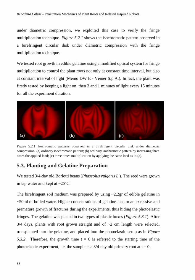
Benedetta Calusi – Penetration Mechanics of Plant Roots and Related Inspired Robots
88
under diametric compression, we exploited this case to verify the fringe
multiplication technique. Figure 5.2.1 shows the isochromatic pattern observed in
a birefringent circular disk under diametric compression with the fringe
multiplication technique.
We tested root growth in edible gelatine using a modified optical system for fringe
multiplication to control the plant roots not only at constant time interval, but also
at constant interval of light (Memo DW E - Vemer S.p.A.). In fact, the plant was
firstly tested by keeping a light on, then 3 and 1 minutes of light every 15 minutes
for all the experiment duration.
Figure 5.2.1 Isochromatic patterns observed in a birefringent circular disk under diametric
compression. (a) ordinary isochromatic pattern; (b) ordinary isochromatic pattern by increasing three
times the applied load; (c) three times multiplication by applying the same load as in (a).
5.3. Planting and Gelatine Preparation
We tested 3/4-day old Borlotti beans (Phaseolus vulgaris L.). The seed were grown
in tap water and kept at ~25˚C.
The birefringent soil medium was prepared by using ~2.2gr of edible gelatine in
~50ml of boiled water. Higher concentrations of gelatine lead to an excessive and
premature growth of fractures during the experiments, thus hiding the photoelastic
fringes. The gelatine was placed in two types of plastic boxes (Figure 5.3.1). After
3/4 days, plants with root grown straight and of ~2 cm length were selected,
transplanted into the gelatine, and placed into the photoelastic setup as in Figure
5.3.2. Therefore, the growth time t = 0 is referred to the starting time of the
photoelastic experiment, i.e. the sample is a 3/4-day old primary root at t = 0.
(a) (b) (c)
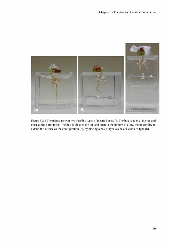
• Chapter 5 • Planting and Gelatine Preparation
89
Figure 5.3.1 The plants grow in two possible types of plastic boxes. (a) The box is open at the top and
close at the bottom; (b) The box is close at the top and open to the bottom to allow the possibility to
extend the surface as the configuration (c), by placing a box of type (a) beside a box of type (b).
(a) (b) (c)
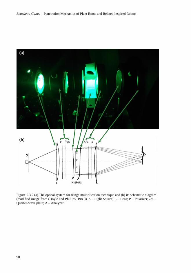
Benedetta Calusi – Penetration Mechanics of Plant Roots and Related Inspired Robots
90
Figure 5.3.2 (a) The optical system for fringe multiplication technique and (b) its schematic diagram
(modified image from (Doyle and Phillips, 1989)). S – Light Source; L – Lens; P – Polarizer; λ/4 –
Quarter-wave plate; A – Analyzer.
(b)
(a)
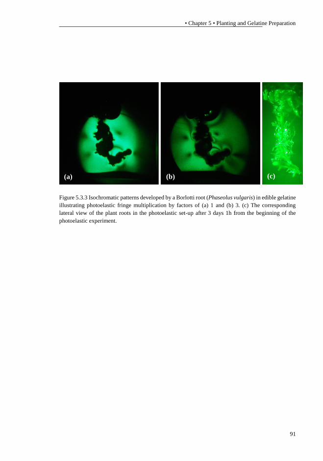
• Chapter 5 • Planting and Gelatine Preparation
91
Figure 5.3.3 Isochromatic patterns developed by a Borlotti root (Phaseolus vulgaris) in edible gelatine
illustrating photoelastic fringe multiplication by factors of (a) 1 and (b) 3. (c) The corresponding
lateral view of the plant roots in the photoelastic set-up after 3 days 1h from the beginning of the
photoelastic experiment.
(a) (b) (c)

Benedetta Calusi – Penetration Mechanics of Plant Roots and Related Inspired Robots
92
Figure 5.3.4 Development of a Borlotti root (Phaseolus vulgaris) in edible gelatine at different growth
times with the root tested by keeping the light on during the all duration of the experiment. See Figure
5.3.3c for the lateral view of the root at t ~ 3 days 1h. The growth time t =0 is the starting time of the
photoelastic experiment, i.e. the sample is a 3/4-day old primary root.
t = 0 t ~ 4h t ~ 1 day 4h
t ~ 2 days 4h t ~ 2 days 7h t ~ 3 days 1h

• Chapter 5 • Planting and Gelatine Preparation
93
Figure 5.3.5 Development of a Borlotti root (Phaseolus vulgaris) in edible gelatine at different growth
times with the root tested by keeping the light on for 3 minutes of light every 15 minutes for all the
experiment duration. On the right the corresponding lateral view of the plant roots in the photoelastic
set-up after 3 days 15h from the beginning of the photoelastic experiment.
Figure 5.3.6 Development of a Borlotti root (Phaseolus vulgaris) in edible gelatine at different growth
times with the root tested by keeping the light on for 1 minutes of light every 15 minutes for all the
experiment duration. On the right the corresponding lateral view of the plant roots in the photoelastic
set-up at t ~ 3 days 18h from the beginning of the photoelastic experiment and just before the arise of
the fracture inside the gelatine.
t ~ 2 days 7h t ~ 2 days 12h t ~ 2 days 14h
t ~ 2 days 21h t ~ 3 days 9h t ~ 3 days 15h
t ~ 4 days
t ~ 3 days 9h
Fracture

Benedetta Calusi – Penetration Mechanics of Plant Roots and Related Inspired Robots
94
5.4. Interpretation and Discussion
We firstly perform preliminary tests to investigate and choose a proper gelatine
concentration and a growing method with the polariscope of our laboratory (the
polariscope has been designed and manufactured at the University of Trento and
used e.g. in (Noselli, Dal Corso and Bigoni, 2010; Misseroni et al., 2014), see
http://ssmg.unitn.it/ for more details). Then, we set up the optical system for fringe
multiplication in order to increase a number of observable fringe order. We applied
the fringe multiplication to the study of plant roots growing in edible gelatine. We
collected the pictures into videos, by monitoring the growth of plant roots in the
fringe multiplication set up keeping the light on at three different time intervals.
We firstly tested keeping the light on for all the duration of the experiment. In this
configuration, roots exhibited an inversion of growth direction with respect to
gravity (Figure 5.3.3, Figure 5.3.4). To verify if the light exposition time could be
a possible consequence of such phenomenon, we modified the photoelastic set-up
to perform the experiments with 3 minutes and 1 minute of light every 15 minutes
for all the experiment duration (Figure 5.3.5 and Figure 5.3.6, respectively). Figure
5.3.6 shows the method with 1 minute of light every 15 minutes may result less
invasive at reversing the green light response of the root with respect the other two
methods.
To give a descriptive explanation of the presence of homogeneous fringes along the
root lateral surface, we exploited the theoretical model developed in Chapter 2 with
the growth data of Phytagel E. In fact, by consider the root growth as consecutive
cycles of Fracture and Regrowth as in Chapter 2 and through the experimental
position of the first fringe, we can obtain an estimated value of the fringe constant
fσ, e.g. at the end of the FRC. The variation of the first fringe position along the root
lateral surface during a FRC is given by Figure 5.4.1. Then, the increase of fringes
along the lateral surface of the root is due to the simultaneous growth of lateral
roots and fractures of the gelatine (Figure 5.3.3c). We are aware that both the
theoretical model and the photoelastic technique do not take into account all the
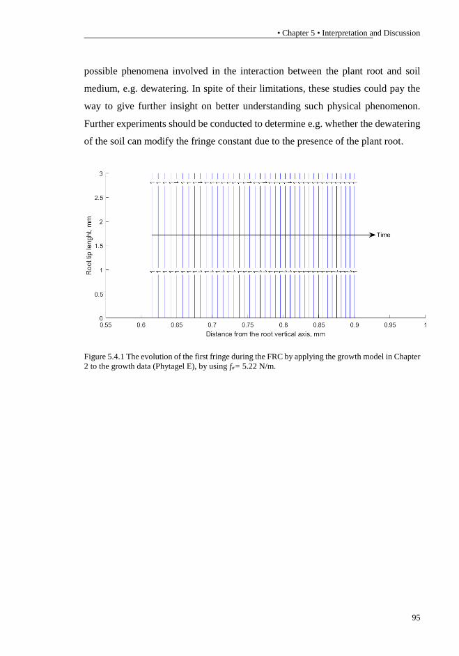
• Chapter 5 • Interpretation and Discussion
95
possible phenomena involved in the interaction between the plant root and soil
medium, e.g. dewatering. In spite of their limitations, these studies could pay the
way to give further insight on better understanding such physical phenomenon.
Further experiments should be conducted to determine e.g. whether the dewatering
of the soil can modify the fringe constant due to the presence of the plant root.
Figure 5.4.1 The evolution of the first fringe during the FRC by applying the growth model in Chapter
2 to the growth data (Phytagel E), by using fσ= 5.22 N/m.

Benedetta Calusi – Penetration Mechanics of Plant Roots and Related Inspired Robots
96
Chapter 6
6. Conclusion and Future Perspective
Animals and plants are in direct contact with the environment and have to face
continuously several unexpected constraints and changes. On this basis, the
exploitation of the movement efficiency adopted by Nature could be a key feature
to provide new bioinspired concepts. Therefore, the interest of science and
engineering is increasing to understand the principles exploited by Nature.
The present thesis aims at creating a synergy between different fields, such as
biology, engineering and mathematics in order to investigate on the adaptive
strategies adopted by plant roots for new potential devices. In particular,
mathematical models applied to plant science can be crucial for both explaining
biological phenomena and better designing robotic systems enabled with
penetration capabilities and adaptive movements. There is a great potential for a
possible extension of such models to develop new methodologies for robots with
adaptive movements based on soft materials. In the present work, both the
theoretical and experimental studies could lead to deeper investigations to gain a
better understanding of the adaptive strategies of plant roots to the outer stimuli.
In Chapter 2, we studied the growth of plant roots in artificial and real soils. Since
the ability of plant roots to penetrate soils is affected by the mechanical stresses
exerted by the surrounding medium, we investigated and modelled the
biomechanical response of the Zea mays L. primary roots, grown in soils with
different impedances. In this regard, we developed a growth mathematical model
based on a modified version of the extended universal law of West, Brown, and
Enquist. Our model, in agreement with our experimental results, showed a different
root elongation compared to data from both real and artificial soil by varying the
soil medium compactness.

• Chapter 6 • Conclusion and Future Perspective
97
Then, in Chapter 3 we extended the mathematical model, developed in Chapter 2,
to the growth of plant roots in artificial soils with different concentrations of
nutrient. In order to avoid the soil heterogeneity, we used experiments in artificial
soil with only the presence of different nutrient stimuli. In fact, we proposed a
model, in combination with experimental data, in order to better understand the
adaptation process of roots in presence of high nutrient concentrations. Our findings
indicated that the root length decreases whereas its radius increases in higher
nutrient concentration. The theoretical framework aims at coupling continuum
mechanics with plant roots response to nutrient availability.
Understanding the mechanisms that control root growth is essential to model the
key biological processes and translate them into possible bio-inspired engineering
applications. Therefore, the two theoretical studies may provide further insights
into the adaptive ability of plant roots at various impedance and nutrient constraints
and could be improved by including and considering a more complete and complex
scenario of the root growth inside a soil medium.
In addition, some theories and hypotheses about the function of the root tip and the
mechanism of transmitted stimuli by the tip along the whole root have not been
completely understood and explained. The investigation of how the mechanical and
surface properties could vary with respect to the outer stimuli is closely related to
the role of root tip as a “motor zone” (Dougal, 1987). Thus, in Chapter 4, we used
the dynamic nanoindentation technique and wettability tests to study the
mechanical properties and surface features of Zea mays L. root tissues. As new cells
are continuously created in the apical region, the cellular differentiation is at an
early stage, close to the root tip. Therefore, the results of the mechanical tests could
reveal root penetration strategies during the growth from the tip. The combination
of soft and stiff materials may enhance plant roots to simultaneously penetrate and
adapt to soil constraints. Accordingly, this experimental study could improve the
current knowledge in the tip function to control the adaptive mechanisms for the
development of bioinspired engineering applications. Future developments will be
Benedetta Calusi – Penetration Mechanics of Plant Roots and Related Inspired Robots
98
the study of the whole plant tissues in various plant species in order to gain a better
understanding of the role of mechanical tissue properties in penetrating soil at
different outer stimuli.
Finally, in Chapter 5, we presented a set-up for the primary root growth in
homogeneous birefringent media using photoelastic technique. An accurate picture
of stress distribution at various points in a photoelastic material can be determined,
by studying the fringe pattern by means of photoelastic technique. Several attempts
have been made due to the difficulties of controlling bacterial activities and gelatine
concentration. Lastly, we obtained a working method to use edible gelatine as a
growing medium for Phaseolus vulgaris primary roots. We selected optical
products for the fringe multiplication technique in order to improve the results on
observable fringe order. Further experiments, exploiting the created non-standard
boxes, could be useful to investigate how the penetration angle of the root could
evolve during the penetration with different soil constraints, e.g. as the tip-to-barrier
angle (observed in (Popova, Tonazzini, et al., 2016)). This study showed that
photoelasticity may be an alternative and potentially useful technique to investigate
the primary root growth. In fact, despite its exploratory nature, this study could
offer some insights into the stress distribution developed by roots inside a
birefringent medium thanks to the monitoring of the root growth by keeping the
light on at different time interval.
• Bibliography •
99
Bibliography
Agrawal, R., Peng, B. and Espinosa, H. D. (2009) ‘Experimental-computational
investigation of ZnO nanowires strength and fracture’, Nano Letters, 9(12), pp.
4177–4183. doi: 10.1021/nl9023885.
Agudelo, C., Packirisamy, M. and Geitmann, A. (2016) ‘Influence of Electric
Fields and Conductivity on Pollen Tube Growth assessed via Electrical Lab-on-
Chip’, Scientific Reports. Nature Publishing Group, 6(January), pp. 1–15. doi:
10.1038/srep19812.
Alessa, L. and Earnhart, C. (2000) ‘Effects of soil compaction on root and root
hair morphology: implications for campsite rehabilitation’, in Wilderness science
in a time of change conference-Volume 5: Wilderness ecosystems, threats, and
management, pp. 99–104.
Atwell, B. (1989) ‘Physiological responses of lupin roots to soil compaction’, in
Loughamn, B. C., Gašparíková, O., and Kolek, J. (eds) Structural and Functional
Aspects of Transport in Roots: Third International Symposium on ‘Structure and
Function of Roots’ Nitra, Czechoslovakia, 3–7 August 1987. Kluwer Academic
Publishers, pp. 251–255.
Baluska, F. et al. (1993) ‘Cellular Dimorphism in the Maize Root Cortex :
Involvement of Microtubules , Ethylene and Gibberellin in the Differentiation of
Cellular Behaviour in Postmitotic Growth Zones’, pp. 394–403.
Baluška, F., Jasik, J., et al. (2001) ‘Latrunculin B-induced plant dwarfism: Plant
cell elongation is F-actin-dependent’, Developmental Biology. doi:
10.1006/dbio.2000.0115.
Baluška, F., Busti, E., et al. (2001) ‘Lilliputian mutant of maize lacks cell
elongation and shows defects in organization of actin cytoskeleton’,
Developmental Biology, 236(2), pp. 478–491. doi: 10.1006/dbio.2001.0333.
Baluška, F. et al. (2009) ‘The “root-brain” hypothesis of Charles and Francis
Darwin’, Plant Signaling & Behavior, 4(12), pp. 1121–1127. doi:
10.4161/psb.4.12.10574.
Baluska, F., Hauskrecht, D. V. M. and Barlow, P. W. (1996) ‘Root Cap Mucilage
and Extracellular Calcium as Modulators of Cellular Growth in Postmitotic
Growth Zones of the Maize Root Apex *’, 109, pp. 25–34.
Baluska, F., Parker, J. S. and Barlow, P. W. (1993) ‘A role for gibberellic-acid in
orienting microtubules and regulating cell-growth polarity in the maize root
cortex.’, Planta, 191(2), pp. 149–157.
Benedetta Calusi – Penetration Mechanics of Plant Roots and Related Inspired Robots
100
Baluška, F., Parker, J. S. and Barlow, P. W. (1993) ‘The microtubular
cytoskeleton in cells of cold-treated roots of maize (Zea mays L.) shows tissue-
specific responses’, Protoplasma, 172(2–4), pp. 84–96. doi:
10.1007/BF01379366.
Bar-Cohen, Y. (2006) ‘Biomimetics - Using nature to inspire human innovation’,
Bioinspiration and Biomimetics. doi: 10.1088/1748-3182/1/1/P01.
Barley, K. P. (1963) ‘Influence of soil strength of growth of roots’, Soil Science,
96(3), pp. 175–180. doi: 10.1097/00010694-196309000-00004.
Bartsch, M. et al. (2001) ‘Exploring Insect Biomechanics with Micromachined
Force Sensors’, Transducers ’01 Eurosensors XV, pp. 1634–1637.
Bartsch, M. S. et al. (2003) ‘Small insect measurements using a custom MEMS
force sensor’, in TRANSDUCERS 2003 - 12th International Conference on Solid-
State Sensors, Actuators and Microsystems, Digest of Technical Papers, pp.
1039–1042. doi: 10.1109/SENSOR.2003.1216946.
Bartsch, M. S. et al. (2007) ‘A multiaxis force sensor for the study of insect
biomechanics’, Journal of Microelectromechanical Systems, 16(3), pp. 709–718.
doi: 10.1109/JMEMS.2007.893677.
Bengough, A. G. et al. (2006) ‘Root responses to soil physical conditions; growth
dynamics from field to cell’, in Journal of Experimental Botany, pp. 437–447.
doi: 10.1093/jxb/erj003.
Bengough, A. G. et al. (2011) ‘Root elongation, water stress, and mechanical
impedance: A review of limiting stresses and beneficial root tip traits’, Journal of
Experimental Botany, pp. 59–68. doi: 10.1093/jxb/erq350.
Bengough, A. G. (2012) ‘Root elongation is restricted by axial but not by radial
pressures: So what happens in field soil?’, Plant and Soil, 360(1–2), pp. 15–18.
doi: 10.1007/s11104-012-1428-8.
Bengough, A. G., Croser, C. and Pritchard, J. (1997) ‘A biophysical analysis of
root growth under mechanical stress’, Plant and Soil, 189(1), pp. 155–164. doi:
10.1023/A:1004240706284.
Bengough, A. G. and Mackenzie, C. J. (1994) ‘Simultaneous measurement of root
force and elongation for seedling pea roots’, Journal of Experimental Botany,
45(1), pp. 95–102. doi: 10.1093/jxb/45.1.95.
Bengough, A. G. and Mullins, C. E. (1990) ‘Mechanical impedance to root
growth: a review of experimental techniques and root growth responses’, Journal
of Soil Science, 41(3), pp. 341–358. doi: 10.1111/j.1365-2389.1990.tb00070.x.
Bengough, A. and Mullins, C. (1990) ‘Mechanical impedance to root growth: a
review of experimental techniques and root growth responses’, Journal of soil
• Bibliography •
101
science, 41, pp. 341–358. doi: 10.1111/j.1365-2389.1990.tb00070.x.
Bennet, R., Breen, C. and Fey, M. (1985a) ‘Aluminium uptake sites in the
primary root of Zea mays L.’, South African Journal of Plant and Soil, 2(1), pp.
1–7.
Bennet, R., Breen, C. and Fey, M. (1985b) ‘The primary site of aluminium injury
in the root of Zea mays L.’, South African Journal of Plant and Soil, 2(1), pp. 8–
17.
Bernardino, N. R., Blickle, V. and Dietrich, S. (2010) ‘Wetting of surfaces
covered by elastic hairs’, Langmuir, 26(10), pp. 7233–7241. doi:
10.1021/la904345r.
Bettencourt, L. M. A. et al. (2007) ‘Growth, innovation, scaling, and the pace of
life in cities’, Proceedings of the National Academy of Sciences, 104(17), pp.
7301–7306. doi: 10.1073/pnas.0610172104.
Bizet, F. et al. (2016) ‘3D deformation field in growing plant roots reveals both
mechanical and biological responses to axial mechanical forces’, Journal of
Experimental Botany, 67(19), pp. 5605–5614. doi: 10.1093/jxb/erw320.
Blengino Albrieu, J. L., Reginato, J. C. and Tarzia, D. A. (2015) ‘Modeling water
uptake by a root system growing in a fixed soil volume’, Applied Mathematical
Modelling. doi: 10.1016/j.apm.2014.11.042.
Bombelli, P., Howe, C. J. and Bertocchini, F. (2017) ‘Polyethylene bio-
degradation by caterpillars of the wax moth Galleria mellonella’, Current Biology,
pp. R292–R293. doi: 10.1016/j.cub.2017.02.060.
Bowles, J. E. (1997) Foundation Analysis and Design, Engineering Geology. doi:
10.1016/0013-7952(84)90010-3.
Bradshaw, A. D. (1965) ‘Evolutionary Significance of Phenotypic Plasticity in
Plants’, Advances in Genetics, 13(C), pp. 115–155. doi: 10.1016/S0065-
2660(08)60048-6.
Brett, P. N. et al. (1995) ‘Automatic Surgical Tools for Penetrating Flexible
Tissues’, IEEE Engineering in Medicine and Biology Magazine, 14(3), pp. 264–
270. doi: 10.1109/51.391778.
Budíková, S. (1999) ‘Structural changes and aluminium distribution in maize root
tissues’, Biologia Plantarum, 42(2), pp. 259–266. doi:
10.1023/A:1002116803679.
Chavarría-Krauser, A., Jäger, W. and Schurr, U. (2005) ‘Primary root growth: A
biophysical model of auxin-related control’, Functional Plant Biology. doi:
10.1071/FP05033.
Benedetta Calusi – Penetration Mechanics of Plant Roots and Related Inspired Robots
102
Clark, L. J. et al. (1996) ‘Complete mechanical impedance increases the turgor of
cells in the apex of pea roots’, Plant, Cell and Environment, 19(9), pp. 1099–
1102. doi: 10.1111/j.1365-3040.1996.tb00217.x.
Clark, L. J. et al. (1999) ‘Maximum axial root growth pressure in pea seedlings:
Effects of measurement techniques and cultivars’, Plant and Soil, 209(1), pp.
101–109. doi: 10.1023/A:1004568714789.
Clark, L. J., Whalley, W. R. and Barraclough, P. B. (2003) ‘How do roots
penetrate strong soil?’, in Plant and Soil, pp. 93–104. doi:
10.1023/A:1026140122848.
Colombi, T. et al. (2017) ‘Root Tip Shape Governs Root Elongation Rate under
Increased Soil Strength’, Plant Physiology, 174(4), pp. 2289–2301. doi:
10.1104/pp.17.00357.
Cranford, S. W. et al. (2012) ‘Nonlinear material behaviour of spider silk yields
robust webs’, Nature, pp. 72–76. doi: 10.1038/nature10739.
Crick, J. C. and Grime, J. P. (1987) ‘Morphological plasticity and mineral nutrient
capture in two herbaceous species of contrasted ecology’, New Phytologist,
107(2), pp. 403–414. doi: 10.1111/j.1469-8137.1987.tb00192.x.
Crouzy, B., Edmaier, K. and Perona, P. (2014) ‘Biomechanics of plant anchorage
at early development stage’, Journal of Theoretical Biology, 363, pp. 22–29. doi:
10.1016/j.jtbi.2014.07.034.
Dally, J. and Riley, W. (1991) Experimental Stress Analysis. Third Edit. McGraw
Hill.
Darwin, C. and Darwin, F. (1880) The power of movement in plants, The Power
of Movement in Plants. doi: 10.1017/CBO9780511693670.
Das, B. M. (2014) Advanced Soil Mechanics 4th edition, CRC press, Taylor &
Francis Group. doi: 10.1029/EO066i042p00714-02.
Dexter, A. R. (1987) ‘Mechanics of root growth’, Plant and Soil, 98(3), pp. 303–
312. doi: 10.1007/BF02378351.
Dietrich, D. et al. (2017) ‘Root hydrotropism is controlled via a cortex-specific
growth mechanism’, Nature Plants. doi: 10.1038/nplants.2017.57.
Dorgan, K. M., Arwade, S. R. and Jumars, P. A. (2007) ‘Burrowing in marine
muds by crack propagation: kinematics and forces’, Journal of Experimental
Biology, 210(23), pp. 4198–4212. doi: 10.1242/jeb.010371.
Dorgan, K. M., Law, C. J. and Rouse, G. W. (2013) ‘Meandering worms :
mechanics of undulatory burrowing in muds’, Proceedings of the Royal Society
B: Biological Sciences, 280(February), pp. 1–9. doi:

• Bibliography •
103
http://dx.doi.org/10.1098/rspb.2012.2948.
Dougal, D. T. (1987) ‘The curvature of Roots’, Botanical Gazette, 23(5), pp. 307–
366.
Doyle, J. F. and Phillips, J. W. (1989) ‘Manual on Experimental Stress Analysis
Fifth Edition Society for Experimental Mechanics’, Society for Experimental.
Drew, M. C. and Saker, L. R. (1978) ‘Nutrient supply and the growth of the
seminal root system in barley: III. Compensatory increases in growth of lateral
roots, and in rates of phosphate uptake, in response to a localized supply of
phosphate’, Journal of Experimental Botany, 29(2), pp. 435–451. doi:
10.1093/jxb/29.2.435.
Dupuy, L., Gregory, P. J. and Bengough, A. G. (2010) ‘Root growth models:
Towards a new generation of continuous approaches’, Journal of Experimental
Botany. doi: 10.1093/jxb/erp389.
Durelli, A. and Riley, W. (1965) Introduction to Photomechanics. Prentice-Hall.
Dyson, R. J. and Jensen, O. E. (2010) ‘A fibre-reinforced fluid model of
anisotropic plant cell growth’, Journal of Fluid Mechanics. doi:
10.1017/S002211201000100X.
Edmaier, K. et al. (2014) ‘Influence of root characteristics and soil variables on
the uprooting mechanics of Avena sativa and Medicago sativa seedlings’, Earth
Surface Processes and Landforms, 39(10), pp. 1354–1364. doi: 10.1002/esp.3587.
Filleur, S. et al. (2005) ‘Nitrate and glutamate sensing by plant roots.’,
Biochemical Society transactions, 33(Pt 1), pp. 283–6. doi:
10.1042/BST0330283.
Foehse, D. and Jungk, A. (1983) ‘Influence of phosphate and nitrate supply on
root hair formation of rape, spinach and tomato plants’, Plant and Soil, 74(3), pp.
359–368. doi: 10.1007/BF02181353.
Forterre, Y. (2013) ‘Slow, fast and furious: Understanding the physics of plant
movements’, Journal of Experimental Botany, pp. 4745–4760. doi:
10.1093/jxb/ert230.
Full, R. J. (2002) ‘Quantifying Dynamic Stability and Maneuverability in Legged
Locomotion’, Integrative and Comparative Biology, 42(1), pp. 149–157. doi:
10.1093/icb/42.1.149.
Full, R., Yamauchi, a and Jindrich, D. (1995) ‘Maximum single leg force
production: cockroaches righting on photoelastic gelatin’, The Journal of
experimental biology, 198(Pt 12), pp. 2441–2452. Available at:
http://www.ncbi.nlm.nih.gov/pubmed/9320366.
Benedetta Calusi – Penetration Mechanics of Plant Roots and Related Inspired Robots
104
Gagliano, M. (2017) ‘The mind of plants: Thinking the unthinkable’,
Communicative & Integrative Biology. Taylor & Francis, 10(2), p. e1288333. doi:
10.1080/19420889.2017.1288333.
Gilroy, S. and Masson, P. (2008) Plant Tropisms. Blackwell Publishing.
Goldman, D. I. and Hu, D. L. (2010) ‘Wiggling Through the World - The
mechanics of slithering locomotion depend on the surroundings’, American
Scientist, 98, pp. 314–323.
Goodman, A. M. and Ennos, A. R. (1999) ‘The effects of soil bulk density on the
morphology and anchorage mechanics of the root systems of sunflower and
maize’, Annals of Botany, 83(3), pp. 293–302. doi: 10.1006/anbo.1998.0822.
Goriely, A. and Neukirch, S. (2006) ‘Mechanics of climbing and attachment in
twining plants’, Physical Review Letters, 97(18). doi:
10.1103/PhysRevLett.97.184302.
Greacen, E. L. and Oh, J. S. (1972) ‘Physics of root growth’, Nature New
Biology, 235(53), pp. 24–25. doi: 10.1038/newbio235024a0.
Grime, J. P. and Mackey, J. M. L. (2002) ‘The role of plasticity in resource
capture by plants’, Evolutionary Ecology, 16(3), pp. 299–307. doi:
10.1023/A:1019640813676.
Gross, K. L., Peters, A. and Pregitzer, K. S. (1993) ‘Fine root growth and
demographic responses to nutrient patches in four old-field plant species’,
Oecologia, 95(1), pp. 61–64. doi: 10.1007/BF00649507.
Guiot, C., Pugno, N. and Delsanto, P. P. (2006) ‘Elastomechanical model of
tumor invasion’, Applied Physics Letters, 89(23), pp. 23–25. doi:
10.1063/1.2398910.
Hamant, O., Traas, J. and Boudaoud, A. (2010) ‘Regulation of shape and
patterning in plant development’, Current Opinion in Genetics and Development.
doi: 10.1016/j.gde.2010.04.009.
Hamza, O. et al. (2006) ‘Biomechanics of Plant Roots: estimating Localised
Deformation with Particle Image Velocimetry’, Biosystems Engineering, 94(1),
pp. 119–132. doi: 10.1016/j.biosystemseng.2006.02.006.
Harris, J. K. (1978) ‘A photoelastic substrate technique for dynamic
measurements of forces exerted by moving organisms’, Journal of Microscopy,
114(2), pp. 219–228. doi: 10.1111/j.1365-2818.1978.tb00132.x.
Hawkes, E. W. et al. (2014) ‘Human climbing with efficiently scaled gecko-
inspired dry adhesives’, Journal of The Royal Society Interface, 12(102), pp.
20140675–20140675. doi: 10.1098/rsif.2014.0675.

• Bibliography •
105
Herbert, E. G. et al. (2009) ‘Measuring the constitutive behavior of viscoelastic
solids in the time and frequency domain using flat punch nanoindentation’,
Journal of Materials Research, 24(3), pp. 626–637. doi: 10.1557/jmr.2009.0089.
Herbert, E. G., Oliver, W. C. and Pharr, G. M. (2008) ‘Nanoindentation and the
dynamic characterization of viscoelastic solids’, Journal of Physics D: Applied
Physics, 41(7). doi: 10.1088/0022-3727/41/7/074021.
Hu, David and Shelley, M. (2012) ‘Slithering Locomotion’, Natural locomotion
in fluids and on surfaces; swimming, flying and sliding, 155, pp. 35–51. doi:
10.1007/978-1-4614-3997-4.
Huang, C. X. and van Steveninck, R. F. M. (1990) ‘Salinity induced structural
changes in meristematic cells of barley roots’, New Phytologist, 115(1), pp. 17–
22. doi: 10.1111/j.1469-8137.1990.tb00916.x.
Isnard, S. and Silk, W. K. (2009) ‘Moving with climbing plants from Charles
Darwin’s time into the 21st century’, American Journal of Botany, pp. 1205–
1221. doi: 10.3732/ajb.0900045.
Jackson, R. B. and Caldwell, M. M. (1989) ‘The timing and degree of root
proliferation in fertile-soil microsites for three cold-desert perennials’, Oecologia,
81(2), pp. 149–153. doi: 10.1007/BF00379798.
Jackson, R. B. and Caldwell, M. M. (1996) ‘Integrating Resource Heterogeneity
and Plant Plasticity: Modelling Nitrate and Phosphate Uptake in a Patchy Soil
Environment’, The Journal of Ecology, 84(6), p. 891. doi: 10.2307/2960560.
Jiang, L. and Feng, L. (2010) Bioinspired Intelligent Nanostructured Interfacial
Materials. World Scientific Publishing Co. Pte. Ltd. and Chemical Industry Press.
Kavalenka, M. N. et al. (2017) ‘Adaptable bioinspired special wetting surface for
multifunctional oil/water separation’, Scientific Reports, 7. doi:
10.1038/srep39970.
Keyes, S. D. et al. (2016) ‘Mapping soil deformation around plant roots using in
vivo 4D X-ray Computed Tomography and Digital Volume Correlation’, Journal
of Biomechanics. Elsevier, 49(9), pp. 1802–1811. doi:
10.1016/j.jbiomech.2016.04.023.
Kirby, J. and Bengough, A. (2002) ‘Influence of soil strength on root growth :
experiments and analysis using a critical-state model’, European Journal of Soil
Science, 53(March), pp. 119–128. doi: 10.1046/j.1365-2389.2002.00429.x.
Kolb, E., Hartmann, C. and Genet, P. (2012) ‘Radial force development during
root growth measured by photoelasticity’, Plant and Soil, 360(1–2), pp. 19–35.
doi: 10.1007/s11104-012-1316-2.
Kolb, E., Legué, V. and Bogeat-Triboulot, M. B. (2017) ‘Physical root-soil
Benedetta Calusi – Penetration Mechanics of Plant Roots and Related Inspired Robots
106
interactions’, Physical Biology, 14(6). doi: 10.1088/1478-3975/aa90dd.
Kurth, E. et al. (1986) ‘Effects of NaCl and CaCl2 on Cell Enlargement and Cell
Production in Cotton Roots’, PLANT PHYSIOLOGY, 82(4), pp. 1102–1106. doi:
10.1104/pp.82.4.1102.
Kynast, R. (2012) ‘Handbook of maize: its biology’, in. Bennetzen Jeff L., Hake
Sarah C. eds. 2009 . Springer, pp. vii–viii.
Laschi, C. et al. (2012) ‘Soft robot arm inspired by the octopus’, Advanced
Robotics, 26(7), pp. 709–727. doi: 10.1163/156855312X626343.
Li, H. et al. (2014) ‘Histone acetylation associated up-regulation of the cell wall
related genes is involved in salt stress induced maize root swelling’, BMC Plant
Biology, 14(1). doi: 10.1186/1471-2229-14-105.
Loades, K. W. et al. (2013) ‘Biomechanics of nodal, seminal and lateral roots of
barley: Effects of diameter, waterlogging and mechanical impedance’, Plant and
Soil, 370(1–2), pp. 407–418. doi: 10.1007/s11104-013-1643-y.
Loades, K. W. et al. (2015) ‘Effect of root age on the biomechanics of seminal
and nodal roots of barley (Hordeum vulgare L.) in contrasting soil environments’,
Plant and Soil, 395(1–2), pp. 253–261. doi: 10.1007/s11104-015-2560-z.
Lockhart, J. A. (1965) ‘An analysis of irreversible plant cell elongation’, Journal
of Theoretical Biology, 8(2), pp. 264–275. doi: 10.1016/0022-5193(65)90077-9.
Margheri, L. et al. (2011) ‘Non-invasive study of Octopus vulgaris arm
morphology using ultrasound’, Journal of Experimental Biology, 214(22), pp.
3727–3731. doi: 10.1242/jeb.057323.
Materechera, S. A., Dexter, A. R. and Alston, A. M. (1991) ‘Penetration of very
strong soils by seedling roots of different plant species’, Plant and Soil, 135(1),
pp. 31–41. doi: 10.1007/BF00014776.
Mazzolai, B. (2017) ‘Plant-inspired growing robots’, Biosystems and Biorobotics,
17, pp. 57–63. doi: 10.1007/978-3-319-46460-2_8.
Mazzolai, B., Beccai, L. and Mattoli, V. (2014) ‘Plants as Model in Biomimetics
and Biorobotics: New Perspectives’, Frontiers in Bioengineering and
Biotechnology, 2. doi: 10.3389/fbioe.2014.00002.
Mirbagheri, S. A. et al. (2015) ‘Sensitively Photoelastic Biocompatible Gelatin
Spheres for Investigation of Locomotion in Granular Media’, Experimental
Mechanics, 55(2), pp. 427–438. doi: 10.1007/s11340-014-9958-z.
Misra, R. K., Dexter, A. R. and Alston, A. M. (1986) ‘Maximum axial and radial
growth pressures of plant roots’, Plant and Soil, 95(3), pp. 315–326. doi:
10.1007/BF02374612.

• Bibliography •
107
Misseroni, D. et al. (2014) ‘Stress concentration near stiff inclusions: Validation
of rigid inclusion model and boundary layers by means of photoelasticity’,
Engineering Fracture Mechanics, 121–122, pp. 87–97. doi:
10.1016/j.engfracmech.2014.03.004.
Mock, U. et al. (2005) ‘Towards ultrahydrophobic surfaces: A biomimetic
approach’, Journal of Physics Condensed Matter, 17(9). doi: 10.1088/0953-
8984/17/9/021.
Murashige, T. and Skoog, F. (1962) ‘A Revised Medium for Rapid Growth and
Bio Assays with Tobacco Tissue Cultures’, Physiologia Plantarum. doi:
10.1111/j.1399-3054.1962.tb08052.x.
Nezhad, A. S. et al. (2013) ‘Quantification of the Young’s modulus of the
primary plant cell wall using Bending-Lab-On-Chip (BLOC)’, Lab on a Chip,
13(13), p. 2599. doi: 10.1039/c3lc00012e.
Niklas, K. J. (1999) ‘The mechanical role of bark’, American Journal of Botany,
86(4), pp. 465–469. doi: Doi 10.2307/2656806.
Normand, V. et al. (2000) ‘New insight into agarose gel mechanical properties.’,
Biomacromolecules. doi: 10.1021/bm005583j.
Noselli, G., Dal Corso, F. and Bigoni, D. (2010) ‘The stress intensity near a
stiffener disclosed by photoelasticity’, International Journal of Fracture, 166(1–
2), pp. 91–103. doi: 10.1007/s10704-010-9502-9.
Okada, K. and Shimura, Y. (1990) ‘Reversible Root Tip Rotation in Arabidopsis
Seedlings Induced by Obstacle-Touching Stimulus’, Science, 250(4978), pp. 274–
276. doi: 10.1126/science.250.4978.274.
Otten, A. and Herminghaus, S. (2004) ‘How Plants Keep Dry: A Physicist’s Point
of View’, Langmuir, 20(6), pp. 2405–2408. doi: 10.1021/la034961d.
Pantano, M. F. et al. (2015) ‘Multiphysics Design and Implementation of a
Microsystem for Displacement-controlled tensile testing of nanomaterials’,
Meccanica, 50, pp. 549–560.
Peaucelle, A. (2014) ‘AFM-based Mapping of the Elastic Properties of Cell
Walls: at Tissue, Cellular, and Subcellular Resolutions’, Journal of Visualized
Experiments. doi: 10.3791/51317.
Pelesko, J. and Bernstein, D. (2003) Modeling MEMS and NEMS. Boca Raton,
FL: Chapman & Hall/CRC.
Pharr, G. M., Oliver, W. C. and Brotzen, F. R. (1992) ‘On the generality of the
relationship among cantact stiffness,contact area, and elastic-modulus during
indentation’, Journal of Materials Research, 7(3), pp. 613–617. doi:
10.1557/JMR.1992.0613.

Benedetta Calusi – Penetration Mechanics of Plant Roots and Related Inspired Robots
108
Pierret, A. et al. (2007) ‘Root Functional Architecture: A Framework for
Modeling the Interplay between Roots and Soil’, Vadose Zone Journal, 6(2), p.
269. doi: 10.2136/vzj2006.0067.
Pietola, L. and Smucker, A. J. M. (1998) ‘Fibrous carrot root responses to
irrigation and compaction of sandy and organic soils’, Plant and Soil, 200(1), pp.
95–105. doi: 10.1023/A:1004294330427.
Pope, M. T. et al. (2017) ‘A Multimodal Robot for Perching and Climbing on
Vertical Outdoor Surfaces’, IEEE Transactions on Robotics, 33(1), pp. 38–48.
doi: 10.1109/TRO.2016.2623346.
Popova, L., van Dusschoten, D., et al. (2016) ‘Plant root tortuosity: an indicator
of root path formation in soil with different composition and density’, Annals of
Botany, 118(4), pp. 685–698. doi: 10.1093/aob/mcw057.
Popova, L., Tonazzini, A., et al. (2016) ‘Unveiling the kinematics of the
avoidance response in maize (Zen mays) primary roots’, Biologia (Poland), 71(2),
pp. 161–168. doi: 10.1515/biolog-2016-0022.
Post, D. (1955) ‘Isochromatic fringe sharpening and fringe multiplication in
photoelasticity’, Proc. SESA, 12(2).
Post, D. (1966) ‘Fringe multiplication in three-dimensional photoelasticity’, The
Journal of Strain Analysis for Engineering Design, 1(5), pp. 380–388. doi:
10.1243/03093247V015380.
Post, D. (1970) ‘Photoelastic-fringe multiplication-For tenfold increase in
sensitivity - Author concludes that fringe multiplication offers economy and
improved accuracy of results’, Experimental Mechanics, 10(8), pp. 305–312. doi:
10.1007/BF02320808.
Potocka, I. and Szymanowska-Pułka, J. (2018) ‘Morphological responses of plant
roots to mechanical stress’, Annals of Botany, (May), pp. 1–13. doi:
10.1093/aob/mcy010.
Roppolo, D. et al. (2011) ‘A novel protein family mediates Casparian strip
formation in the endodermis’, Nature, 473(7347), pp. 381–384. doi:
10.1038/nature10070.
Sadeghi, A. et al. (2014) ‘A novel growing device inspired by plant root soil
penetration behaviors’, PLoS ONE, 9(2), pp. 1–10. doi:
10.1371/journal.pone.0090139.
Sadeghi, A. et al. (2017) ‘A plant-inspired robot with soft differential bending
capabilities’, Bioinspiration and Biomimetics. IOP Publishing, 12(1). doi:
10.1088/1748-3190/12/1/015001.
Sánchez-Calderón, L., Ibarra-Cortés, M. E. and Zepeda-Jazo, I. (2013) ‘Root

• Bibliography •
109
Development and Abiotic Stress Adaptation’, in Agricultural and Biological
Sciences, ‘Abiotic Stress - Plant Responses and Applications in Agriculture’. doi:
10.5772/55043.
Schiavi, A., Cuccaro, R. and Troia, A. (2016) ‘Strain-rate and temperature
dependent material properties of Agar and Gellan Gum used in biomedical
applications’, Journal of the Mechanical Behavior of Biomedical Materials, 53,
pp. 119–130. doi: 10.1016/j.jmbbm.2015.08.011.
Silverberg, J. L. et al. (2012) ‘3D imaging and mechanical modeling of helical
buckling in Medicago truncatula plant roots’, Proceedings of the National
Academy of Sciences, 109(42), pp. 16794–16799. doi: 10.1073/pnas.1209287109.
Strogatz, S. (2000) ‘Nonlinear dynamics and chaos: with applications to physics,
biology, chemistry and engineering’, Cambridge, MA: Westview Press. Available
at: http://www.citeulike.org/group/4585/article/2606929%5Cnpapers://30dd8192-
3a85-4010-af1a-3e33b620a902/Paper/p7760.
Taiz, L. and Zeiger, E. (1991) Plant physiology, EE. UU. California: Sinauer.
Available at: http://pdf115.nikubooks.com/plant-physiology-fifth-edition-PDF-
341715.pdf.
Tan, T. H. et al. (2015) ‘How grow-and-switch gravitropism generates root
coiling and root waving growth responses in Medicago truncatula’, Proceedings
of the National Academy of Sciences, 112(42), pp. 12938–12943. doi:
10.1073/pnas.1509942112.
Taylor, H. M. and Ratliff, L. F. (1969) ‘Root elongation rates of cotton and
peanuts as a function of soil strength and soil water content’, Soil Science, 108(2),
pp. 113–119. doi: 10.1097/00010694-196908000-00006.
Tian, X. and Doerner, P. (2013) ‘Root resource foraging: does it matter?’,
Frontiers in Plant Science, 4. doi: 10.3389/fpls.2013.00303.
Tomlinson, R. A. and Taylor, Z. A. (2015) ‘Photoelastic materials and methods
for tissue biomechanics applications’, Optical Engineering, 54(8), p. 081208. doi:
10.1117/1.OE.54.8.081208.
Tramacere, F. et al. (2014) ‘Hairy suckers: The surface microstructure and its
possible functional significance in the octopus vulgaris sucker’, Beilstein Journal
of Nanotechnology, 5(1), pp. 561–565. doi: 10.3762/bjnano.5.66.
Tricinci, O. et al. (2015) ‘3D Micropatterned Surface Inspired by Salvinia molesta
via Direct Laser Lithography’, ACS Applied Materials and Interfaces, 7(46), pp.
25560–25567. doi: 10.1021/acsami.5b07722.
Volkmar, K. M. (1994) ‘Pre-germination effects on mechanically impeded root
growth of barley (Hordeum vulgare L)’, Plant and Soil, 163(2), pp. 197–202. doi:

Benedetta Calusi – Penetration Mechanics of Plant Roots and Related Inspired Robots
110
10.1007/BF00007968.
Wang, J. et al. (2017) ‘Bioinspired shape-memory graphene film with tunable
wettability’, Science Advances. doi: 10.1126/sciadv.1700004.
Wei, C. and Lintilhac, P. M. (2007) ‘Loss of Stability: A New Look at the Physics
of Cell Wall Behavior during Plant Cell Growth’, PLANT PHYSIOLOGY, 145(3),
pp. 763–772. doi: 10.1104/pp.107.101964.
Wendell, D. M. et al. (2012) ‘Experimental Investigation of Plant Root Growth
Through Granular Substrates’, Experimental Mechanics, 52(7), pp. 945–949. doi:
10.1007/s11340-011-9569-x.
West, G. B., Brown, J. H. and Enquist, B. J. (1997) ‘A general model for the
origin of allometric scaling laws in biology’, Science. doi:
10.1126/science.276.5309.122.
West, G. B., Brown, J. H. and Enquist, B. J. (2001) ‘A general model for
ontogenetic growth’, Nature, 413(6856), pp. 628–631. doi: 10.1038/35098076.
Whiteley, G. M. and Dexter, A. R. (1981) ‘Elastic response of the roots of field
crops’, Physiologia Plantarum, 51(4), pp. 407–417. doi: 10.1111/j.1399-
3054.1981.tb05578.x.
Wilson, A. J. and Robards, A. W. (1978) ‘The ultrastructural development of
mechanically impeded barley roots. Effects on the endodermis and pericycle’,
Protoplasma, 95(3), pp. 255–265. doi: 10.1007/BF01294454.
Wilson, A. J., Robards, A. W. and Goss, M. J. (1977) ‘Effects of mechanical
impedance on root growth in barley, Hordeum vulgare L.: II. Effects on cell
development in seminal roots’, Journal of Experimental Botany, 28(5), pp. 1216–
1227. doi: 10.1093/jxb/28.5.1216.
Yang, Y., Chen, L. and Li, N. (2016) ‘How gauge length and loading rate
influence the root tensile strength of Betula platyphylla’, Journal of Soil and
Water Conservation, 71(6), pp. 460–466. doi: 10.2489/jswc.71.6.460.
Zacarias, L. and Reid, M. S. (1992) ‘Inhibition of ethylene action prevents root
penetration through compressed media in tomato (Lycopersicon esculentum)
seedlings’, Physiologia Plantarum, 86(2), pp. 301–307. doi: 10.1034/j.1399-
3054.1992.860217.x.
Zeiger, C. et al. (2017) ‘Selective filtration of oil/water mixtures with bioinspired
porous membranes’, RSC Adv., 7(52), pp. 32806–32811. doi:
10.1039/C7RA05385A.
Zha, G. et al. (2016) ‘Mechanical touch responses of Arabidopsis TCH1-3 mutant
roots on inclined hard-agar surface’, International Agrophysics, 30(1), pp. 105–
111. doi: 10.1515/intag-2015-0065.

• Bibliography •
111
Zhu, M. Y., Ahn, S. J. and Matsumoto, H. (2003) ‘Inhibition of growth and
development of root border cells in wheat by Al’, Physiologia Plantarum, 117(3),
pp. 359–367. doi: 10.1034/j.1399-3054.2003.00036.x.
Zidan, I., Azaizeh, H. and Neumann, P. M. (1990) ‘Does Salinity Reduce Growth
in Maize Root Epidermal Cells by Inhibiting Their Capacity for Cell Wall
Acidification?’, PLANT PHYSIOLOGY, 93(1), pp. 7–11. doi: 10.1104/pp.93.1.7.

Benedetta Calusi – Penetration Mechanics of Plant Roots and Related Inspired Robots
112
• Appendix • Additional Related Activity: Load Sensor Instability in MEMS-based Tensile Testing
Devices
113
Appendix
A. Additional Related Activity: Load Sensor Instability
in MEMS-based Tensile Testing Devices
Quantitative and qualitative approaches involve experiments at the different length
scales from micro/nanoscale to macroscale in the context of biomechanics and
biomimetics.
The ability of animal and plant movements and how their tissues adapt to external
constraints and changes can be collected through experimental data. Experimental
methods can be tissue mechanical tests and surface properties characterizations.
Mechanical tests include nanoindentation, tensile and compression tests that
provide information about the strength, stiffness, and hardness of the considered
tissues. Indeed, such properties affect the ability of the whole animal/plant structure
to perform specific movements. The aim of such experiments is to unlock the
secrets of the biological tissue structures that could significantly affect the stability
of movements and anchorage. While the second type of characterization will
provide information about wettability and adhesion of the tissue during a specific
movement. To this aim direct measurements of animal ground forces and plant
ground anchorages can be carried out by means of force sensors and tracking tools
to study the adaptive movement ability of plants and animals as a whole, see e.g.
the Full and Tu force platform at Berkeley (Bartsch et al., 2001, 2003, 2007), the
Bending-Lab-On-Chip and the Electrical Lab-on-Chip (Nezhad et al., 2013;
Agudelo, Packirisamy and Geitmann, 2016). In addition, mathematical modelling
is useful to analyse and verify the plausibility of experimental findings. Theoretical
frameworks have a key role to highlight and explain natural phenomena in several
fields. Moreover, an analytical approach can be useful in potential predictions for
performances of bio- and non-bioinspired devices. In fact, dynamical systems
theory could shed light on the potential implementation of strategies adopted by
Nature into the physical key parameters of novel devices, e.g. to prevent the
Benedetta Calusi – Penetration Mechanics of Plant Roots and Related Inspired Robots
114
possible onset of instability in devices during measurements (Agrawal, Peng and
Espinosa, 2009).
In this regard, MEMS-based tensile testing devices are very powerful tools for
mechanical characterization of nanoscale materials, as they allow for testing of
micro/nano-sized components in situ electron microscopes. In a typical
configuration, they consist of an actuator, to deliver force/displacement, and a load
sensor, which is connected to the sample like springs in series. Such configuration,
while providing a high-resolution force measurement, can cause the onset of
instability phenomena, which can later compromise the test validity. In the present
Chapter, such phenomena are quantitatively discussed through the development of
an analytical model, which allows to find a relationship between the rise of
instability and the sensor stiffness, which is the key parameter to be optimized. In
addition, a potential bio-inspired design can be an effective solution to avoid such
instability phenomena.
The work in this Chapter arises from the collaboration with Dr. Ing. Maria Fiorella
Pantano of the University of Trento.
Analytical modeling of MEMS-based tensile testing devices
In most of MEMS tensile testing devices, the load sensor and the sample to be tested
are connected like springs in series, as in the lumped parameters model reported in
Figure A.1a. This is a 2-degrees-of-freedom system, where the sample is
represented as a spring with a generic characteristic (its mass is negligible with
respect to that of the load sensor), while the load sensor is modeled through a mass
(MLS) connected to the substrate through a damper (with damping constant D) and
a spring (with spring constant kLS). The sample undergoes a displacement xS, as a
consequence of the actuator movement (not reported in the present model), whereas
xLS is the load sensor's displacement.
For simplicity, let us first neglect both the damping and inertial contribution, and
let us evaluate the global force-displacement relationship characterizing the system
comprising the load sensor and sample springs (Figure A.1b).

• Appendix • Additional Related Activity: Load Sensor Instability in MEMS-based Tensile Testing
Devices
115
Figure A.1 a) Lumped parameters model of a typical tensile testing device, where the sample can be
modeled like a spring whose characteristic shows a softening branch; b) Global behavior of the system
consisting of both the load sensor and the sample, showing the relationship between the force (F)
corresponding to the applied displacement (xS). When the sample enters in the softening regime, F
may increase (line a)) or decrease (either line b) or c)) with xS, depending on the magnitude of the
slope of the sample characteristic, ∂F/∂(xS-xLS), compared to the load sensor stiffness, kLS. In
particular, line b) corresponds to ∂F/∂(xS-xLS)<0 and kLS>|∂F/∂(xS-xLS)|, c) ∂F/∂(xS-xLS)<0 and
kLS<|∂F/∂(xS-xLS)|. In order to evaluate the stability of the equilibrium position of the load sensor, its
dynamic behavior can be linearized and modeled about such position through a Jacobian matrix. c)
The sign of the trace, τ, and the determinant, Δ, of the Jacobian matrix determine the stability of the
equilibrium point.
Global system behavior
The overall deformation undergone by the system is xS=xLS+ (xS-xLS), where xLS is
the load sensor deformation and (xS-xLS) the sample deformation. If infinitely small
displacements are considered, the overall system deformation becomes:
𝑑𝑥𝑆 = 𝑑𝑥𝐿𝑆 + 𝑑(𝑥𝑆 − 𝑥𝐿𝑆). (A1)
Since kLS is the load sensor spring constant, then dxLS=dF/kLS. If a general
characteristic is assumed for the sample, it follows that 𝑑(𝑥𝑆 − 𝑥𝐿𝑆) =
𝜕(𝑥𝑆 − 𝑥𝐿𝑆) 𝜕𝐹⁄ 𝑑𝐹, where dF is the force acting on the system, which is the same
on both the sample and load sensor (since they are connected in series). Thus, eq.
(A1) can be rewritten as:

Benedetta Calusi – Penetration Mechanics of Plant Roots and Related Inspired Robots
116
𝑑𝑥𝑆 =𝑑𝐹
𝑘𝐿𝑆+𝜕(𝑥𝑆 − 𝑥𝐿𝑆)
𝜕𝐹dF , (A2)
or,
𝑑𝑥𝑆𝑑𝐹
=1
𝑘𝐿𝑆+𝜕(𝑥𝑆 − 𝑥𝐿𝑆)
𝜕𝐹 . (A3)
At the beginning, the sample characteristic has a linear increasing trend, (e.g., ∂(xS-
xLS)/∂F or ∂F/∂(xS-xLS) are constant, and the sample can be modeled like a linear
spring), and the slope of the system characteristic (∂F/∂xS) is equal to the equivalent
stiffness of the sample and load sensor spring constants. Then, the system
characteristic may either increase or decrease with increasing xS, depending on the
sample’s behavior. In particular, either of the following cases may occur (Figure
A.1b):
(a) Overall system hardening as a consequence of sample hardening, e.g, if ∂(xS-
xLS)/∂F>0;
(b) Overall softening with negative slope, if the sample exhibits softening (e.g.,
∂F/∂(xS-xLS)<0) and its slope in modulus is smaller than the load sensor spring
constant. In fact, from eq. (A3):
𝑑𝑥𝑆𝑑𝐹
< 0 ⇔1
𝑘𝐿𝑆+𝜕(𝑥𝑆 − 𝑥𝐿𝑆)
𝜕𝐹< 0 , (𝐴4)
which is equivalent to
𝑘𝐿𝑆 > |𝜕𝐹
𝜕(𝑥𝑆 − 𝑥𝐿𝑆)|, (𝐴5)
(c) Overall softening with positive slope if the sample exhibits softening (e.g.,
∂F/∂(xs-xLS)<0) and its slope in modulus is bigger than the load sensor spring
constant. In fact, from eq. (A3):

• Appendix • Additional Related Activity: Load Sensor Instability in MEMS-based Tensile Testing
Devices
117
𝑑𝑥𝑆𝑑𝐹
> 0 ⇔1
𝑘𝐿𝑆+𝜕(𝑥𝑆 − 𝑥𝐿𝑆)
𝜕𝐹> 0 , (𝐴5)
which is equivalent to
𝑘𝐿𝑆 < |𝜕𝐹
𝜕(𝑥𝑆 − 𝑥𝐿𝑆)|. (𝐴7)
Thus, in this latter case, the system would tend to come back to smaller values of
xS, displaying a snap-back branch with positive slope. However, since in a typical
tensile test, xS is progressively increased, the sample is broken without the
possibility to follow the snap-back branch and, thus, the corresponding region of
the sample characteristic. As a consequence, the optimal design value for the load
sensor stiffness depends on the steepest point of interest to be expected during
softening regime in the sample characteristic curve. Thus, as a compromise
between high resolution during the elastic regime and stability requirement, we can
define an optimal load sensor stiffness as
𝑘𝐿𝑆,𝑜𝑝𝑡 = 𝜂 |𝜕𝐹
𝜕(𝑥𝑆 − 𝑥𝐿𝑆)|𝑀𝐴𝑋
,
where η is a partial factor for stability, which could be set equal to 10%.
Load sensor stability
It is now interesting to study what happens to the load sensor when its stiffness is
smaller than the sample characteristic slope during softening. To this aim, it is
convenient to refer to the model depicted in Figure A.1a and write the load sensor’s
equilibrium equation:
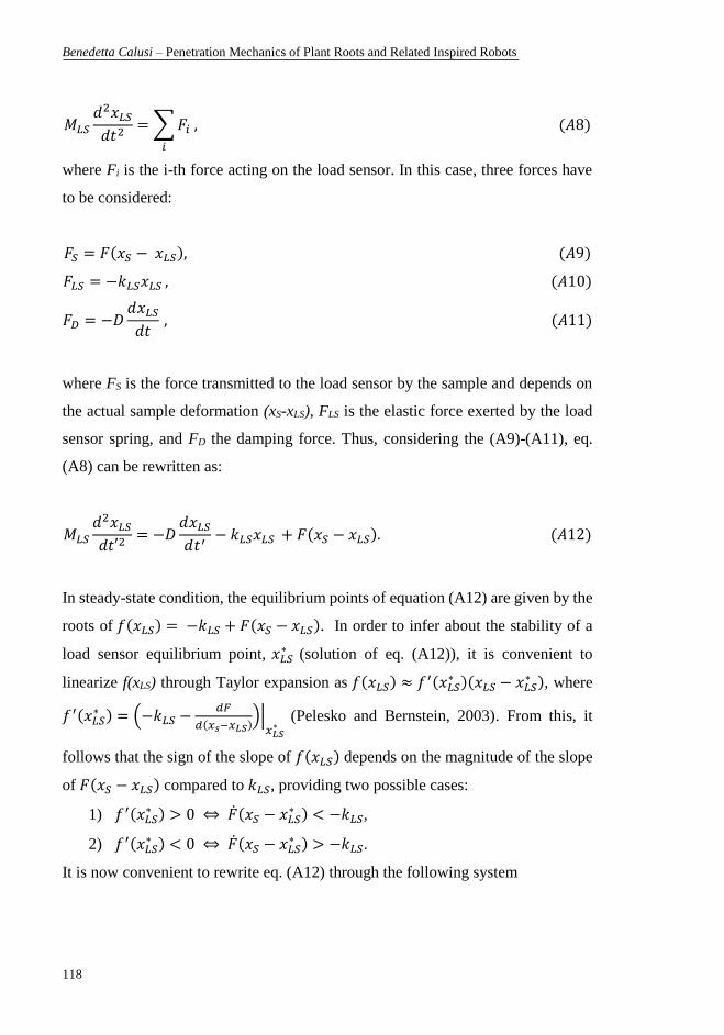
Benedetta Calusi – Penetration Mechanics of Plant Roots and Related Inspired Robots
118
𝑀𝐿𝑆𝑑2𝑥𝐿𝑆𝑑𝑡2
=∑𝐹𝑖 , (𝐴8)
𝑖
where Fi is the i-th force acting on the load sensor. In this case, three forces have
to be considered:
𝐹𝑆 = 𝐹(𝑥𝑆 − 𝑥𝐿𝑆), (𝐴9)
𝐹𝐿𝑆 = −𝑘𝐿𝑆𝑥𝐿𝑆 , (𝐴10)
𝐹𝐷 = −𝐷𝑑𝑥𝐿𝑆𝑑𝑡
, (𝐴11)
where FS is the force transmitted to the load sensor by the sample and depends on
the actual sample deformation (xS-xLS), FLS is the elastic force exerted by the load
sensor spring, and FD the damping force. Thus, considering the (A9)-(A11), eq.
(A8) can be rewritten as:
𝑀𝐿𝑆
𝑑2𝑥𝐿𝑆𝑑𝑡′2
= −𝐷𝑑𝑥𝐿𝑆𝑑𝑡′
− 𝑘𝐿𝑆𝑥𝐿𝑆 + 𝐹(𝑥𝑆 − 𝑥𝐿𝑆). (𝐴12)
In steady-state condition, the equilibrium points of equation (A12) are given by the
roots of 𝑓(𝑥𝐿𝑆) = −𝑘𝐿𝑆 + 𝐹(𝑥𝑆 − 𝑥𝐿𝑆). In order to infer about the stability of a
load sensor equilibrium point, 𝑥𝐿𝑆∗ (solution of eq. (A12)), it is convenient to
linearize f(xLS) through Taylor expansion as 𝑓(𝑥𝐿𝑆) ≈ 𝑓′(𝑥𝐿𝑆
∗ )(𝑥𝐿𝑆 − 𝑥𝐿𝑆∗ ), where
𝑓′(𝑥𝐿𝑆∗ ) = (−𝑘𝐿𝑆 −
𝑑𝐹
𝑑(𝑥𝑠−𝑥𝐿𝑆))|𝑥𝐿𝑆∗
(Pelesko and Bernstein, 2003). From this, it
follows that the sign of the slope of 𝑓(𝑥𝐿𝑆) depends on the magnitude of the slope
of 𝐹(𝑥𝑆 − 𝑥𝐿𝑆) compared to 𝑘𝐿𝑆, providing two possible cases:
1) 𝑓′(𝑥𝐿𝑆∗ ) > 0 ⇔ �̇�(𝑥𝑆 − 𝑥𝐿𝑆
∗ ) < −𝑘𝐿𝑆,
2) 𝑓′(𝑥𝐿𝑆∗ ) < 0 ⇔ �̇�(𝑥𝑆 − 𝑥𝐿𝑆
∗ ) > −𝑘𝐿𝑆.
It is now convenient to rewrite eq. (A12) through the following system
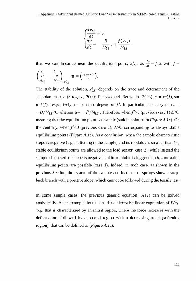
• Appendix • Additional Related Activity: Load Sensor Instability in MEMS-based Tensile Testing
Devices
119
{
𝑑𝑥𝐿𝑆𝑑𝑡
= 𝑣,
𝑑𝑣
𝑑𝑡= −
𝐷
𝑀𝐿𝑆𝑣 +
𝑓(𝑥𝐿𝑆)
𝑀𝐿𝑆,
that we can linearize near the equilibrium point, 𝑥𝐿𝑆∗ , as
𝑑𝒖
𝑑𝑡= 𝐽 𝒖, with 𝐽 =
(0 1𝑓′
𝑀𝐿𝑆−
𝐷
𝑀𝐿𝑆
)|𝑥𝐿𝑆∗
, 𝒖 = (𝑥𝐿𝑆−𝑥𝐿𝑆∗
𝑣).
The stability of the solution, 𝑥𝐿𝑆∗ , depends on the trace and determinant of the
Jacobian matrix (Strogatz, 2000; Pelesko and Bernstein, 2003), 𝜏 = 𝑡𝑟(𝐽), ∆=
𝑑𝑒𝑡(𝐽), respectively, that on turn depend on 𝑓′. In particular, in our system 𝜏 =
−𝐷 𝑀𝐿𝑆⁄ <0, whereas ∆= −𝑓′ 𝑀𝐿𝑆⁄ . Therefore, when 𝑓′>0 (previous case 1) Δ<0,
meaning that the equilibrium point is unstable (saddle point from Figure A.1c). On
the contrary, when 𝑓′<0 (previous case 2), Δ>0, corresponding to always stable
equilibrium points (Figure A.1c). As a conclusion, when the sample characteristic
slope is negative (e.g., softening in the sample) and its modulus is smaller than kLS,
stable equilibrium points are allowed to the load sensor (case 2); while instead the
sample characteristic slope is negative and its modulus is bigger than kLS, no stable
equilibrium points are possible (case 1). Indeed, in such case, as shown in the
previous Section, the system of the sample and load sensor springs show a snap-
back branch with a positive slope, which cannot be followed during the tensile test.
In some simple cases, the previous generic equation (A12) can be solved
analytically. As an example, let us consider a piecewise linear expression of F(xS-
xLS), that is characterized by an initial region, where the force increases with the
deformation, followed by a second region with a decreasing trend (softening
region), that can be defined as (Figure A.1a):

Benedetta Calusi – Penetration Mechanics of Plant Roots and Related Inspired Robots
120
𝐹(𝑥𝑆 − 𝑥𝐿𝑆)
= {𝑘0(𝑥𝑆 − 𝑥𝐿𝑆), 𝑖𝑓 𝑥𝑆 − 𝑥𝐿𝑆 < 𝑥
∗
𝑘0𝑥∗ − 𝑘1(𝑥𝑆 − 𝑥𝐿𝑆 − 𝑥
∗), 𝑖𝑓 𝑥𝑆 − 𝑥𝐿𝑆 > 𝑥∗ (𝐴13)
Its first region defines the sample elastic regime, while the second one corresponds
to the softening region. In order to study what happens to the sensor as soon as the
sample enters within the softening regime, we substitute the second of equations
(A13) in equation (A12), which then becomes:
𝑀𝐿𝑆
𝑑2𝑥𝐿𝑆𝑑𝑡′2
= −𝐷𝑑𝑥𝐿𝑆𝑑𝑡′
− 𝑘𝐿𝑆𝑥𝐿𝑆 + 𝑘0𝑥∗ − 𝑘1(𝑥𝑆 − 𝑥𝐿𝑆 − 𝑥
∗). (𝐴14)
It is convenient rewrite Eq. (A14) in dimensionless form. To this aim, we introduce
the dimensionless time, t=t’√|𝑘1−𝑘𝐿𝑆|
𝑀𝐿𝑆 , and length, y=xLS/l, being l the sample gage
length and k1≠kLS. With these positions, Eq. (A14) can be rewritten as:
𝑑2𝑦
𝑑𝑡2= −𝛼
𝑑𝑦
𝑑𝑡+ 𝑠𝑔𝑛(𝑘1 − 𝑘𝐿𝑆)𝑦 +
𝑥∗(𝑘0 + 𝑘1) − 𝑘1𝑥𝑆𝑙|𝑘1 − 𝑘𝐿𝑆|
. (𝐴15)
Where 𝛼 =𝐷
√𝑀𝐿𝑆|𝑘1−𝑘𝐿𝑆| is a corrected quality factor, that takes into account the
presence of the sample through the term k1.
Considering a typical MEMS, like that one reported in (Pantano et al., 2015), the
damping contribution can be neglected with respect to the inertial effects, meaning
that α<<1. Thus, in the inertia-dominated regime, Eq. (A15) simplifies as:
𝑑2𝑦
𝑑𝑡2= 𝑠𝑔𝑛(𝑘1 − 𝑘𝐿𝑆)𝑦 +
𝑥∗(𝑘0 + 𝑘1) − 𝑘1𝑥𝑆𝑙|𝑘1 − 𝑘𝐿𝑆|
. (𝐴16)
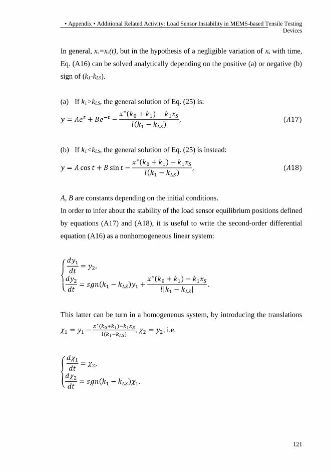
• Appendix • Additional Related Activity: Load Sensor Instability in MEMS-based Tensile Testing
Devices
121
In general, xs=xs(t), but in the hypothesis of a negligible variation of xs with time,
Eq. (A16) can be solved analytically depending on the positive (a) or negative (b)
sign of (k1-kLS).
(a) If k1>kLS, the general solution of Eq. (25) is:
𝑦 = 𝐴𝑒𝑡 + 𝐵𝑒−𝑡 −𝑥∗(𝑘0 + 𝑘1) − 𝑘1𝑥𝑆
𝑙(𝑘1 − 𝑘𝐿𝑆), (𝐴17)
(b) If k1<kLS, the general solution of Eq. (25) is instead:
𝑦 = 𝐴 cos 𝑡 + 𝐵 sin 𝑡 −𝑥∗(𝑘0 + 𝑘1) − 𝑘1𝑥𝑆
𝑙(𝑘1 − 𝑘𝐿𝑆), (𝐴18)
A, B are constants depending on the initial conditions.
In order to infer about the stability of the load sensor equilibrium positions defined
by equations (A17) and (A18), it is useful to write the second-order differential
equation (A16) as a nonhomogeneous linear system:
{
𝑑𝑦1𝑑𝑡
= 𝑦2,
𝑑𝑦2𝑑𝑡
= 𝑠𝑔𝑛(𝑘1 − 𝑘𝐿𝑆)𝑦1 +𝑥∗(𝑘0 + 𝑘1) − 𝑘1𝑥𝑆
𝑙|𝑘1 − 𝑘𝐿𝑆|.
This latter can be turn in a homogeneous system, by introducing the translations
𝜒1 = 𝑦1 −𝑥∗(𝑘0+𝑘1)−𝑘1𝑥𝑆
𝑙(𝑘1−𝑘𝐿𝑆), 𝜒2 = 𝑦2, i.e.
{
𝑑𝜒1𝑑𝑡
= 𝜒2,
𝑑𝜒2𝑑𝑡
= 𝑠𝑔𝑛(𝑘1 − 𝑘𝐿𝑆)𝜒1.

Benedetta Calusi – Penetration Mechanics of Plant Roots and Related Inspired Robots
122
The above homogeneous linear system has a fixed point, χ*, at χ1=0, χ2=0, i.e. the
origin corresponds to the equilibrium position of the system. Repeating the same
logic as before, the trace, τ, and the determinant, Δ, of the Jacobian matrix
associated to the linear system provides the stability of the fixed point. In this case,
τ=0, while Δ=-sgn(k1-kLs). Thus, with reference to Figure A.1c,
(a) If k1>kLS, Δ<0, thus the equilibrium point, χ*, is a saddle point, i.e.,
unstable.
(b) If k1<kLS, Δ>0the equilibrium point, χ*, is a center, i.e., neutrally stable.
Since 𝑑𝐹
𝑑(𝑥𝑠−𝑥𝐿𝑆)= 𝑘1 and k1 represents the slope of the decreasing branch of the
sample characteristic, the results found now match the conclusions derived
previously in case of a sample with a generic characteristic.
The ability of plant roots to penetrate soils is affected by several stimuli from the surrounding medium such as mechanical stresses and chemical changes. Therefore, roots have developed multiple responses to the several outer stimuli. Since plant roots have to face very complex problems to grow deeply into the ground, they are remarkable examples of problem-solving behaviour and adaptation to the outer constraints. The adaptation strategies of a natural root are not yet completely known and understood with exhaustive explanations. For this reason, mathematical models and experimental techniques applied to biological phenomena can perform a key role in translating the Nature adaptive solutions into engineering applications. The aim of this thesis is to provide further insights in understanding biological phenomena for the development of new technologies inspired by the adaptive ability of plant roots. Accordingly, both theoretical and experimental explanations to the adaptive behaviour of plant roots are proposed. The mathematical modelling is based on a modified version of the extended West, Brown and Enquist universal law, considering the root growth as an inclusion problem. The proposed equation has as a particular case a growth equation exploiting an approach similar to Lockhart taking into account the soil impedance. The influence of mechanical stresses and nutrient availability on the root growth are studied. The solutions of the analytical model are compared with experimental data collected in real and artificial soils. In addition, the theories and hypotheses of the root ability to grow in the apical region through nanoindentation, wettability, and photoelasticity are investigated. The first technique provided insights for the possible role and function at both different tissues levels and distances from the tip in the root movement and penetration during the growth. The investigation of root tissue properties revealed that the penetration and adaptation strategies adopted by plant roots could be enhanced by a combination of soft and stiff tissues. The second technique aimed to highlight the wettability of the apical zone and root hairs for the acquisition of water and nutrients. Finally, photoelastic experiments provided a non-invasive and in situ observation of plant roots growth and, by exploiting the fringe multiplication, a set up for the study of plant roots growing in edible gelatine is proposed.